Multihorizon currency returns and Purchasing Power Parity∗

Mikhail Chernov† and Drew Creal‡

April 23, 2018

Abstract

Exposures of expected future depreciation rates to the current interest rate differentialviolate the UIP hypothesis in a distinctive pattern that is a non-monotonic function ofhorizon. Conversely, forward, risk-adjusted expected depreciation rates are monotonic. Weexplain the two patterns by incorporating the weak form of PPP into a no-arbitrage jointmodel of the depreciation rate, inflation differential, domestic and foreign yield curves.Short-term departures from PPP generate the first pattern. The risk premiums for thesedepartures generate the second pattern.

JEL Classification Codes: F31, F47, G12, G15.

Keywords: uncovered interest parity, purchasing power parity, cointegration, multiplehorizons, affine term structure model.

∗ We thank Michael Bauer, Valentin Haddad, Lars Lochstoer, Rob Richmond, Rosen Valchev, andCynthia Wu for comments on earlier drafts and participants in seminars at and conference sponsored byChicago Fed, Copenhagen, Dallas Fed, EDHEC, Erasmus, SITE 2017, Oklahoma, Tinbergen Institute, UTDallas, UCLA Macro-Finance brown bag. The latest version is available at

https://sites.google.com/site/mbchernov/CC_PPP_latest.pdf.† Anderson School of Management, UCLA, NBER, and CEPR; mikhail.chernov@anderson.ucla.edu.‡ Booth School of Business, University of Chicago; dcreal@chicagobooth.edu.

1 Introduction

The literature on foreign exchange (FX) rates has a strong interest in Uncovered InterestParity (UIP) violations, that is, in documenting how their risk premiums vary with the stateof the economy and what are the sources of this variation. More recently, this interest hasexpanded to multiple periods. One bit of evidence is that exposure of the forecasted depre-ciation rate to the respective interest rate differential (IRD) has a puzzling non-monotonicpattern, as a function of the forecast horizon (Bacchetta and van Wincoop, 2010; Engel,2016; Valchev, 2016). In contrast, as we show in this paper, the same exposure of foreignforward rates is monotonic. The two pieces of evidence essentially reflect expectations ofthe same object – future depreciation rates – but under different probabilities, actual versusrisk-adjusted, respectively.

In this paper we ask which features of the data generating process could account for thetwo types of patterns simultaneously. We conclude that incorporating weak, or “long-run”,purchasing power parity (PPP, hereafter) into a joint model of exchange rates and bondprices goes a long way towards this goal. PPP posits that the real exchange rate (RER) isstationary, or, equivalently, that the nominal exchange rate between two countries and theirrespective price levels are cointegrated. The error correction component of this cointegratingrelationship is the driving force behind the empirical success of our model.

The error correction term characterizes how state variables adjust in response to a shock tothe RER in order to restore the long-run relationship between these variables. The speedof this adjustment, which we denote by a parameter alpha, does not matter in the long runbut will affect relationships between the state variables at intermediate horizons. Alphasare responsible for the documented shapes of exchange rate forecasts. Thus, any economictheory that is trying to explain the currency predictability patterns should be focusing ongenerating endogenous speed of error correction.

This conclusion suggests that bond-based evidence should exhibit similar non-monotonicpatterns across horizons. They do not. This is because bond returns or prices reflect risk-adjusted expectations, and UIP holds under the risk-adjusted probability, a.k.a. coveredinterest parity (CIP). This means that the loading on the IRD is equal to one and thatno other variable predicts the depreciation rate one step ahead: the risk-adjusted alphacontrolling the speed of the depreciation rate’s adjustment is equal to zero. This effectleads to a monotonic pattern in exposure to the IRD.

We implement these ideas via a Gaussian no-arbitrage international term structure model.Such models are based on a state that follows VAR-like dynamics. We complement such aVAR by the cointegrating relationship between the nominal exchange rate and the two pricelevels that is implied by PPP. The standard practice is to combine such a relationship withthe VAR dynamics via a VECM representation. We reinterpret the VECM by introducingthe companion form of a VAR and extending the original vector of state variables to includethe new state, that is, the (stationary) RER. Including state variables that are cointegrated

1

into the dynamics of the model is new to the literature on no-arbitrage term structuremodels.

First, we use this modeling framework to illustrate our main points in the context of themost simple setting. The state vector contains the nominal depreciation rate, inflationdifferential and the IRD. Second, we confirm these insights by estimating a realistic modelof the joint behavior of bilateral depreciation rates and yield curves of the two respectivecountries. In this case, the state includes the nominal depreciation rate, the respectiveinflation rates, and nominal interest rates of two countries and of different maturities.

We estimate VARs in bilateral settings of the U.S.A. and one of the following four countries:the U.K., Canada, Germany/Euro, and Japan. In each case the model does a good job incapturing the joint dynamics of the macro variables and term structures of interest rates.In particular, the model replicates the cross-horizon regression patterns with respect toboth actual and risk-adjusted expectations. The model also matches the long-horizon UIPpatterns documented by Chinn and Meredith (2004). Further, we provide evidence thatremoving the PPP-based cointegrating relationship eliminates the model’s ability to matchthe multi-horizon patterns.

Under the null of our model, the IRD-based regressions can be interpreted as projectionsof the nominal FX premium on the IRD. We compare the nominal FX premium impliedby our model and that depends on all the VAR variables to the projected one. The twoexhibit similar cyclical properties regardless of the horizon but the model-based premium islarger and often moves in the direction that is opposite of the projected one. This evidencesuggests that UIP-based intuition about the FX premium behavior could be misleading andthat there are other variables that could play an important role in the premium variationover time.

Related literature

The literature on currency risk premiums is extensive. In this brief review, we focus onpapers that explore the role of the RER in this context. Our paper is most closely relatedto Dahlquist and Penasse (2016), who explore the PPP implications for UIP regressions.They impose PPP by iterating forward the relationship between nominal excess returns,real exchange rates, interest differentials, and inflation differential, a.k.a. the present valueapproach. They do not focus on the role of deviations from PPP at the short to intermediatehorizons, neither do they study the interaction with yield curves.

Engel (2016) uses a VECM with the cointegrating relationship implied by PPP as a tool forconstructing cross-horizon expectations of nominal depreciation rates, but there is no dis-cussion of departures from PPP. Jorda and Taylor (2012) use a similar VECM to motivatepredictive regressions of nominal depreciation rates. Boudoukh, Richardson, and Whitelaw(2016) explore similar regressions. Balduzzi and Chiang (2017) explore the present value

2

approach as a restriction that is helpful in increasing the power of tests of the UIP hypoth-esis. Relatedly, Ferreira Filipe and Maio (2016) use the same restriction to compute vari-ance decompositions of nominal exchange rates. Asness, Moskowitz, and Pedersen (2013);Menkhoff, Sarno, Schmeling, and Schrimpf (2017) use real exchange rates in the cross-section of currencies.

2 Preliminary evidence

2.1 Review of regressions

Let St denote the exchange rate defined in terms of the number of dollars $ per unit offoreign currency. If St increases, the U.S. dollar depreciates. Let `t and t denote the oneperiod U.S. and foreign interbank rates. We use lower case letters to denote the logarithmof a variable, i.e., st = logSt, and hats to denote a variable from a foreign country, i.e.,t. We use ∆st+1 = st+1 − st to denote the one-period time-series difference operator, and

∆c`t = `t− t to denote the cross-country difference operator. We study multiple countries,but we suppress asset-specific notation for simplicity.

The famous uncovered interest parity (UIP) regressions of Bilson (1981); Fama (1984);Tryon (1979) construct forecasts of next period depreciation rates, Et [∆st+1], on the basisof current IRDs. The recent literature, such as Engel (2016); Valchev (2016), focuses onforecasts of depreciation rates at longer horizons. That is, the authors document howEt [∆st+n] changes with horizon n as a function of ∆c`t.

Financial markets also make implicit forecasts of future depreciation rates when they valueforeign and domestic bonds. In contrast to the UIP regressions, these forecasts are produced

under the risk-adjusted probability, E∗t [∆st+n] . Let fyn−1t and fy

n−1

t denote the U.S. andforeign one-period forward interest rates, that is, the rate an investor can lock in at time t

for borrowing from t+ n− 1 to t+ n. The forward exchange rate fsn−1t = fyn−1

t − fyn−1

t

provides a measure of the market’s risk-adjusted expectation of the future depreciation ratefsn−1

t = logE∗t [exp ∆st+n] = E∗t [∆st+n] + convexity. This prompts us to complementthe existing evidence on actual forecasts and to study E∗t [∆st+n] as a function of ∆c`t fordifferent horizons n.

2.2 Data

We work with monthly data from the U.S., U.K., Canada, Germany/Eurozone, and Japanfrom January 1983 to December 2015 making for T = 396 observations per country. Nominalexchange rates are from the Federal Reserve Bank of St. Louis. Prior to the introductionof the Euro, we use the German Deutschemark and splice these series together beginning

3

in 1999. Following a long tradition in the literature, interbank rate differentials ∆c`t areconstructed from forward exchange rates, obtained from Datastream.1 We obtained dailyinterbank rate and exchange rate data and take the last business day of each month.

To analyze the risk-adjusted forecasts, we need forward exchange rates at longer matu-rities. They are constructed from government bond yields, ynt , via fyn−1

t = nynt − (n −1)yn−1

t . U.S. government yields are downloaded from the Federal Reserve and are con-structed by Gurkaynak, Sack, and Wright (2007). All foreign government zero-couponyields are downloaded from their respective central banks (Bank of England, Bundes-bank, Bank of Canada and the Bank of Japan). All government yields have maturitiesof 12, 24, 35, 48, 60, 72, 84, 96, 108, 120 months. Because the available maturities are annual,we can only run regressions on average annual forward rates. The quality, frequency, andavailable maturities of the government bond data dictate the choice of countries in oursample.

2.3 Results

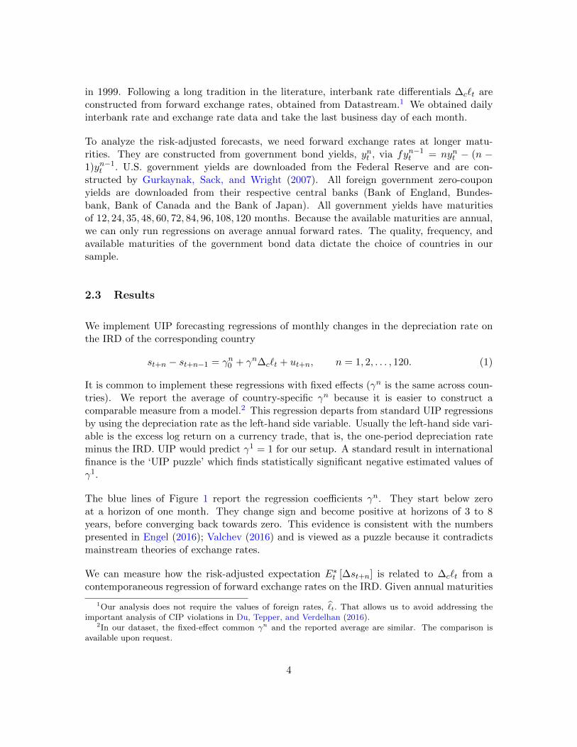
We implement UIP forecasting regressions of monthly changes in the depreciation rate onthe IRD of the corresponding country

st+n − st+n−1 = γn0 + γn∆c`t + ut+n, n = 1, 2, . . . , 120. (1)

It is common to implement these regressions with fixed effects (γn is the same across coun-tries). We report the average of country-specific γn because it is easier to construct acomparable measure from a model.2 This regression departs from standard UIP regressionsby using the depreciation rate as the left-hand side variable. Usually the left-hand side vari-able is the excess log return on a currency trade, that is, the one-period depreciation rateminus the IRD. UIP would predict γ1 = 1 for our setup. A standard result in internationalfinance is the ‘UIP puzzle’ which finds statistically significant negative estimated values ofγ1.

The blue lines of Figure 1 report the regression coefficients γn. They start below zeroat a horizon of one month. They change sign and become positive at horizons of 3 to 8years, before converging back towards zero. This evidence is consistent with the numberspresented in Engel (2016); Valchev (2016) and is viewed as a puzzle because it contradictsmainstream theories of exchange rates.

We can measure how the risk-adjusted expectation E∗t [∆st+n] is related to ∆c`t from acontemporaneous regression of forward exchange rates on the IRD. Given annual maturities

1Our analysis does not require the values of foreign rates, t. That allows us to avoid addressing theimportant analysis of CIP violations in Du, Tepper, and Verdelhan (2016).

2In our dataset, the fixed-effect common γn and the reported average are similar. The comparison isavailable upon request.

4

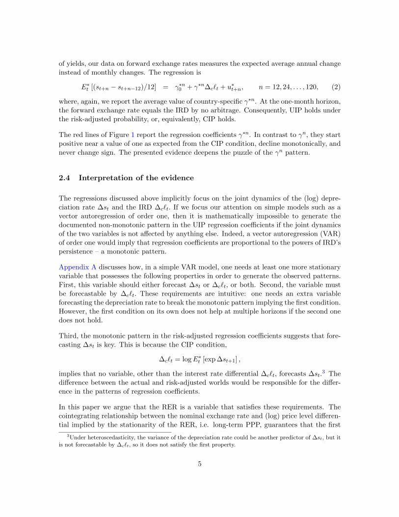
of yields, our data on forward exchange rates measures the expected average annual changeinstead of monthly changes. The regression is

E∗t [(st+n − st+n−12)/12] = γ∗n0 + γ∗n∆c`t + u∗t+n, n = 12, 24, . . . , 120, (2)

where, again, we report the average value of country-specific γ∗n. At the one-month horizon,the forward exchange rate equals the IRD by no arbitrage. Consequently, UIP holds underthe risk-adjusted probability, or, equivalently, CIP holds.

The red lines of Figure 1 report the regression coefficients γ∗n. In contrast to γn, they startpositive near a value of one as expected from the CIP condition, decline monotonically, andnever change sign. The presented evidence deepens the puzzle of the γn pattern.

2.4 Interpretation of the evidence

The regressions discussed above implicitly focus on the joint dynamics of the (log) depre-ciation rate ∆st and the IRD ∆c`t. If we focus our attention on simple models such as avector autoregression of order one, then it is mathematically impossible to generate thedocumented non-monotonic pattern in the UIP regression coefficients if the joint dynamicsof the two variables is not affected by anything else. Indeed, a vector autoregression (VAR)of order one would imply that regression coefficients are proportional to the powers of IRD’spersistence – a monotonic pattern.

Appendix A discusses how, in a simple VAR model, one needs at least one more stationaryvariable that possesses the following properties in order to generate the observed patterns.First, this variable should either forecast ∆st or ∆c`t, or both. Second, the variable mustbe forecastable by ∆c`t. These requirements are intuitive: one needs an extra variableforecasting the depreciation rate to break the monotonic pattern implying the first condition.However, the first condition on its own does not help at multiple horizons if the second onedoes not hold.

Third, the monotonic pattern in the risk-adjusted regression coefficients suggests that fore-casting ∆st is key. This is because the CIP condition,

∆c`t = logE∗t [exp ∆st+1] ,

implies that no variable, other than the interest rate differential ∆c`t, forecasts ∆st.3 The

difference between the actual and risk-adjusted worlds would be responsible for the differ-ence in the patterns of regression coefficients.

In this paper we argue that the RER is a variable that satisfies these requirements. Thecointegrating relationship between the nominal exchange rate and (log) price level differen-tial implied by the stationarity of the RER, i.e. long-term PPP, guarantees that the first

3Under heteroscedasticity, the variance of the depreciation rate could be another predictor of ∆st, but itis not forecastable by ∆c`t, so it does not satisfy the first property.

5

and second properties hold. Risk-adjustment takes care of the rest. In the following, weexplicitly show how it works. While we cannot prove that there are no other variables thatcould satisfy the aforementioned conditions, we argue that none of the variables heretoforeexplored in the literature satisfy these requirements.

3 A simple model

The purpose of this section is to illustrate how the documented regression patterns can bereplicated when the RER serves as a variable that co-moves with the nominal depreciationrate and IRD.

3.1 Error correction representation

We reconcile both actual and risk-adjusted patterns of the regression coefficients by high-lighting the role of the risk of intermediate-term deviations from Purchasing Power Parity(PPP). Short-term PPP states that the RER is equal to one, or, in logs, et ≡ st−pt+pt = 0,where pt denotes the (log) price level. Short-term PPP does not hold empirically but thereis a strong, although not universal, opinion that PPP does hold over the long-term, that is,et is stationary. We assert long-term PPP and show how this helps in understanding theevidence presented in the previous section.

We present a simple model motivated by the specifications of Engel (2016); Dahlquist andPenasse (2016); Jorda and Taylor (2012) that allows us to explain how PPP connects to theevidence. We introduce a vector of non-stationary macro variables mt = (st,∆cpt)

>, where∆cpt = pt − pt. Further, we work with the following stationary variables: domestic andforeign inflation rates πt = ∆pt and πt = ∆pt, and their cross-sectional difference ∆cπt =πt − πt; the IRD ∆c`t. Stack the state variables into a vector ft: ft = (∆m>t ,∆c`t)

>. RERet = β>mmt is stationary, that is, the macro variables mt are cointegrated with cointegratingvector β>m = (1,−1).

Ignoring means (assuming all variables have a zero mean), the state is assumed to follow avector error correction model (VECM):

ft = Φfft−1 + αfet−1 + Σfεt.

Errors in this model are deviations from the cointegrating relation et = 0 (long-term PPP).They set in motion changes in ft that correct the errors. The vector αf = (αs, απ, α`)

>

controls the speed of this error correction.

To simplify the setup, assume that

Φf =

0 0 φs`0 φπ 00 0 φ`

, Σf =

σs 0 00 σπ 00 0 σ`

.

6

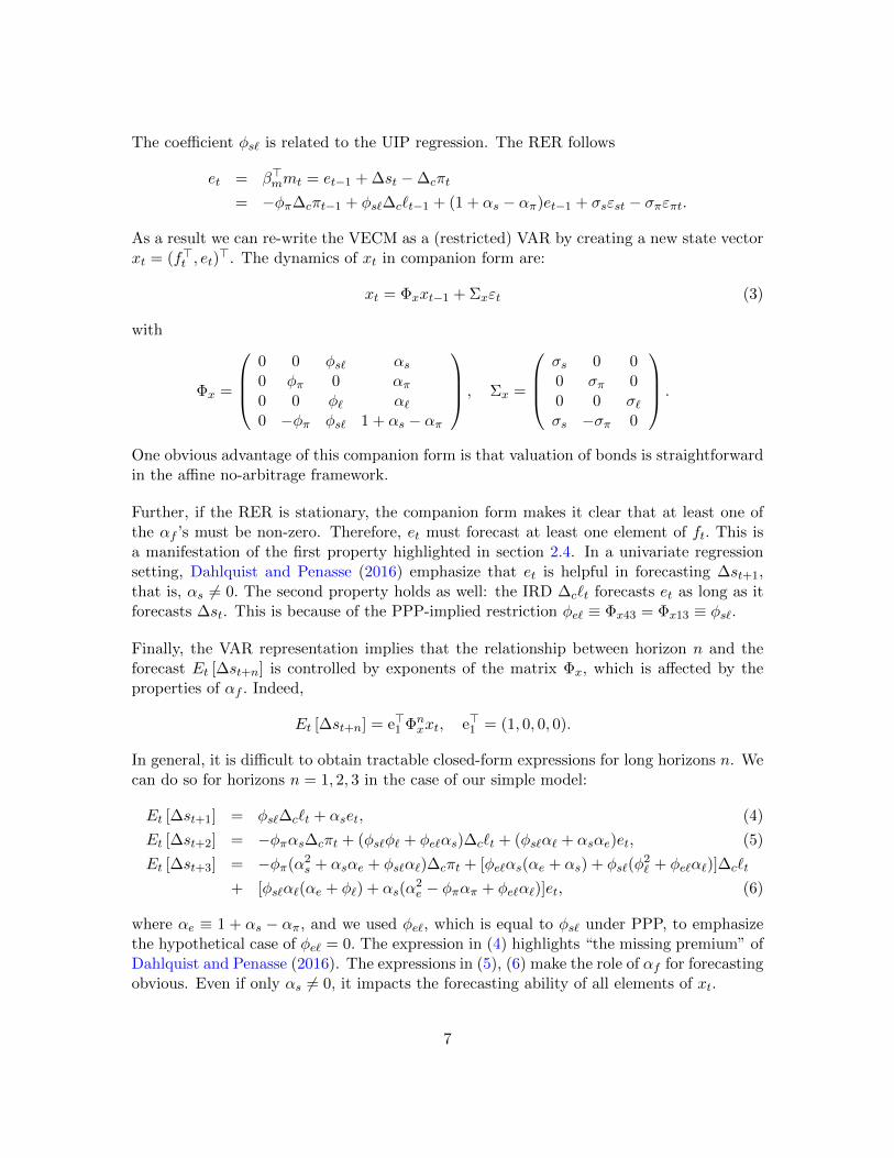
The coefficient φs` is related to the UIP regression. The RER follows

et = β>mmt = et−1 + ∆st −∆cπt

= −φπ∆cπt−1 + φs`∆c`t−1 + (1 + αs − απ)et−1 + σsεst − σπεπt.

As a result we can re-write the VECM as a (restricted) VAR by creating a new state vectorxt = (f>t , et)

>. The dynamics of xt in companion form are:

xt = Φxxt−1 + Σxεt (3)

with

Φx =

0 0 φs` αs0 φπ 0 απ0 0 φ` α`0 −φπ φs` 1 + αs − απ

, Σx =

σs 0 00 σπ 00 0 σ`σs −σπ 0

.

One obvious advantage of this companion form is that valuation of bonds is straightforwardin the affine no-arbitrage framework.

Further, if the RER is stationary, the companion form makes it clear that at least one ofthe αf ’s must be non-zero. Therefore, et must forecast at least one element of ft. This isa manifestation of the first property highlighted in section 2.4. In a univariate regressionsetting, Dahlquist and Penasse (2016) emphasize that et is helpful in forecasting ∆st+1,that is, αs 6= 0. The second property holds as well: the IRD ∆c`t forecasts et as long as itforecasts ∆st. This is because of the PPP-implied restriction φe` ≡ Φx43 = Φx13 ≡ φs`.

Finally, the VAR representation implies that the relationship between horizon n and theforecast Et [∆st+n] is controlled by exponents of the matrix Φx, which is affected by theproperties of αf . Indeed,

Et [∆st+n] = e>1 Φnxxt, e>1 = (1, 0, 0, 0).

In general, it is difficult to obtain tractable closed-form expressions for long horizons n. Wecan do so for horizons n = 1, 2, 3 in the case of our simple model:

Et [∆st+1] = φs`∆c`t + αset, (4)

Et [∆st+2] = −φπαs∆cπt + (φs`φ` + φe`αs)∆c`t + (φs`α` + αsαe)et, (5)

Et [∆st+3] = −φπ(α2s + αsαe + φs`α`)∆cπt + [φe`αs(αe + αs) + φs`(φ

2` + φe`α`)]∆c`t

+ [φs`α`(αe + φ`) + αs(α2e − φπαπ + φe`α`)]et, (6)

where αe ≡ 1 + αs − απ, and we used φe`, which is equal to φs` under PPP, to emphasizethe hypothetical case of φe` = 0. The expression in (4) highlights “the missing premium” ofDahlquist and Penasse (2016). The expressions in (5), (6) make the role of αf for forecastingobvious. Even if only αs 6= 0, it impacts the forecasting ability of all elements of xt.

7

As the horizon increases, the loadings on ∆c`t can be written as the sum of two terms thatare controlled by the forecasting parameters φs` and αf . We highlight these here for n = 3as

term 1 = φs`(φ2` + φe`α`)

term 2 = φe`αs(αe + αs).

The first term contains φs` and it multiplies powers of the IRD autocorrelation coefficientφ2` , which becomes φn−1

` at longer horizons. This term induces a slow monotonic decayin the covariances as the horizon increases and it is the dominant component of the UIPregression coefficients γn, especially at short horizons. If the RER were not present in themodel (αf = 0), or if φe` = 0 then the cross auto-covariance between the depreciation rateand the IRD would simply decay monotonically because it is influenced only by the productφs`φ

n−1` as the horizon increases. These observations are consistent with the properties

outlined in section 2.4.

In order to illustrate these relationships quantitatively, we estimate the VECM in (3) usingthe U.S. and the U.K. data. In the spirit of the previous section, we report the model-impliedcoefficients γn. The results are presented in the left panel of Figure 2.

We consider several scenarios to emphasize the role of αf : (i) all elements of αf are equal tozero; (ii) only one of the elements of αf is not equal to zero; (iii) all the elements of αf arefree. The first case corresponds to the regular VAR for the state ft. It implies the standardpattern of monotonically increasing coefficients that approach zero at long horizons. Thesecond case when απ 6= 0 happens to be almost identical. The coefficients γn cross zero atlong horizons suggesting a potential hump at n > 120 months when α` 6= 0. Finally, whenαs 6= 0 and in the third case, we observe the pattern that is qualitatively consistent withFigure 1.

3.2 Risk adjustment

Our model is too simple to perform a formal risk-adjustment because we do not have anexplicit specification of the reference interest rate `t. Therefore, we follow a storied financetradition and use asterisks to denote parameters that are different under the risk-adjustedprobability. The “volatility” matrix Σf is unchanged. The persistence matrix Φ∗f could bedifferent from Φf , including the zero elements becoming non-zero. For the purposes of thisdiscussion we simplify and assume the following form:

Φ∗x =

0 0 1 00 φ∗π 0 α∗π0 0 φ∗` α∗`0 −φ∗π 1 1− α∗π

.

The first row is dictated by the fact that CIP must hold. The second and third rows areassumed. The last row is implied by the first three.

8

The CIP-imposed restrictions that φ∗s` = 1 and α∗s = 0 immediately suggest that the risk-adjusted pattern could have different properties. Indeed, the risk-adjusted counterparts ofterms 1 and 2 in equation (6) for a forecast horizon n = 3 are:

term 1∗ = φ∗2` + α∗`

term 2∗ = 0.

If α∗` is sufficiently close to zero, we obtain a monotonic pattern in the regression coefficients,γ∗n that starts at a value of one at horizon n = 1 due to CIP.

One needs to use prices of market instruments, e.g., bonds, to estimate the risk-adjustedparameters. We are not going to do that in this section. Instead, we simply assume thatthe state variables are more persistent under the risk-adjusted probability. Thus, we setφ∗` = 0.99 (φ` = 0.97) and φ∗π = 0.5 (φπ = 0.27). We further consider two scenarios witheither α∗π = α∗` = 0, or α∗π = απ and α∗` = α`. We set α∗s = 0 in both scenarios because ofCIP.

The right panel of Figure 2 displays the results. As a benchmark, the red line with crossesshows the actual pattern of γn corresponding to the full VECM model from the left panel.The green line with asterisks corresponds to the case when α∗π = απ and α∗` = α`. Thisline is monotonic but its slope appears to be too small compared to the evidence in Figure1. Most importantly, the values of γ∗n for large n are much higher than the correspondingγn. The black line with squares corresponds to α∗π = α∗` = 0. In this case the pattern isqualitatively much closer to the empirical one.

4 A realistic model

We have presented multihorizon empirical patterns of coefficients that relate actual and risk-adjusted expectations of future depreciation rates to the current IRD. We illustrated, usinga simple model, how these patterns can be captured in one framework by incorporating theRER that converges to PPP in the long run and currency risk premiums. In this sectionwe verify that this intuition actually holds in the data by developing an international no-arbitrage term structure model of nominal yields together with inflation rates, and nominaland real exchange rates.

We follow a plan that is similar to the presentation of the simple model in section 3. We startwith a generic state ft that controls the dynamics of the state variables and follows an errorcorrection model (ECM). We show how it is related to macro variables and, after properlyadjusting for risk premiums, to domestic and foreign bond prices. Then we present a specificchoice of the state ft whose elements are easily interpretable. To the best of our knowledge,the VECM structure for the factors and its companion form are new to the literature on no-arbitrage term structure models. The literature on international no-arbitrage term structuremodels does not incorporate the real exchange rate as a factor.

9

4.1 State dynamics

We specify the dynamics of the state ft as a Gaussian VECM given by

ft = µf + Φfft−1 + ΠffLt−1 + Σfεt εt ∼ N (0, 1) (7)

where fLt denotes the factors in levels. The factors ft are stationary while the levels fLt areunit-root non-stationary. This implies the existence of cointegration and that the matrixof coefficients Πf has reduced rank; see Engle and Granger (1987). It can be factoredas Πf = αfβ

>f where βf is the matrix of cointegrating vectors. The matrix αf contains

the speed of adjustment parameters that determine how fast the system converges back toits long-run equilibrium. Our model of cointegration is an example of an error correctionrepresentation; see, e.g. equation [19.1.42] in Hamilton (1994). Our representation differsfrom the standard approach in the econometrics literature in two ways. We define ft toinclude only I(0) variables rather than a mixture of I(1) and I(0) variables and we definethe matrix of cointegrating vectors βf to include only linear combinations of non-stationaryvariables; see Appendix B for more discussion.

4.1.1 Macro variables

We model the depreciation rate and the inflation rate differential as a linear function of thestate given by

∆st = δs,0 + δ>s,fft (8)

∆cπt = δπ,0 + δ>π,fft. (9)

For convenience, we stack the nominal exchange rates and price level differentials into avector mt = (st ∆cpt)

> and write their first differences ∆mt as a function of the factors as

∆mt = δm,0 + δm,fft. (10)

The initial value m0 = (s0 ∆cp0)> is assumed to be known. The log RER between the U.S.and foreign country is defined as

et ≡ st −∆cpt ≡ β>mmt, (11)

where β>m = (1 − 1).

4.1.2 Companion form of state dynamics

Given the relationship between the macroeconomic variables mt and the state variables ft,the dynamics of the real exchange rates et are pinned down by the dynamics of the factorsft in (7). To see this, we write real exchange rates in terms of the factors

et = β>mmt = et−1 + β>m (δm,0 + δm,fft)

10

and substitute in ft from (7) to find the dynamics of real exchange rates

et = βf,0 + β>f µf + β>f Φfft−1 +(

1 + β>f αf

)et−1 + β>f Σfεt (12)

where β>f = β>mδm,f and βf,0 = β>mδm,0.

Combining (7) and (12), we define the state vector xt =(f>t e>t

)>and write the VECM in

companion VAR form

xt = µx + Φxxt−1 + Σxεt, εt ∼ N (0, 1) , (13)

where the vectors and matrices are defined as

µx =

(µf

βf,0 + β>f µf

)Φx =

(Φf αfβ>f Φf 1 + β>f αf

)Σx =

(Σf

β>f Σf

).

The companion form for xt makes immediately clear that if αf = 0 so that there is nocointegration then the real exchange rate et must be non-stationary. This is because Φx

reduces to a lower block-triangular matrix whose lower right block is simply equal to onewhen αf = 0. The matrix Φx will have (at least) one eigenvalue equal to one. Conversely,if et is stationary, then αf 6= 0 and the real exchange rate must forecast one of the variablesin the system: future depreciation rates, inflation rate differentials, or interest rates.

Most theories of the real exchange rate in the international macroeconomics literature resultin stationary real exchange rates. A natural question to address is which other variable thereal exchange rate forecasts. This point is similar to Cochrane (2008), where the price-to-dividend ratio represents the cointegrating relationship. If it is stationary, then it mustforecast either returns or dividend growth.

4.2 Yields

It is standard practice in the literature to run the UIP regressions using interbank ratesas the one month IRD. While researchers frequently associate these rates with Libor, thisinterpretation is problematic prior to Libor’s inception in 1986 and in the wake of thefinancial crisis of 2008 (Du, Tepper, and Verdelhan, 2016). We describe how we addressthese issues in the implementation section. We refer to the relevant U.S. interbank rate asU.S. Libor, for brevity. We use the U.S. Libor rate as the reference discount rate so that wecould speak to the UIP regressions directly. Subsequently, we derive all other bond pricesrelative to this curve.

11

4.2.1 The stochastic discount factor

We model the dynamics of the log stochastic discount factor (SDF) denominated in termsof the U.S. Libor rate as

logMt,t+1 = −δ`,0 − δ>`,xxt −1

2λ>t λt − λ>t εt+1 (14)

with market prices of risk

λt = Σ−1f (λµ + λφft + λαet) . (15)

See Appendix C.

The physical distribution of the state vector xt implied by (13) together with the stochasticdiscount factor (14) yield the risk-adjusted distribution of xt via p∗(xt+1|xt)/p(xt+1|xt) =Mt,t+1/Et[Mt,t+1]. As a result, risk-adjusted dynamics of xt are given by

xt = µ∗x + Φ∗xxt−1 + Σxεt.

The matrices of parameters under the risk-adjusted probability share a similar form asabove

µ∗x =

(µ∗f

βf,0 + β∗>f µ∗f

)Φ∗x =

(Φ∗f α∗f

β∗>f Φ∗f 1 + β∗>f α∗f

)Σx =

(Σf

β∗>f Σf

)where

µ∗f = µf − λµ Φ∗f = Φf − λφ α∗f = αf − λαThe speed of adjustment parameters αf may carry a risk premium.

In our setting, the matrices containing the cointegrating vectors βf = β∗f are the same acrossprobability measures, which gives the real exchange rate the same definition. It is possibleto write down a more general model where there may exist cointegrating relationshipsacross yields, price levels, exchange rates, and other macroeconomic variables. A researcher

could then estimate(βf , β

∗f

)and test for the presence of cointegrating relationships across

series and across countries. We leave this extension to future research and focus on thesetting where the only cointegrating relationships in the model are those defined by the realexchange rates in (11).

4.2.2 Libor-related rates

The prices of hypothetical zero-coupon U.S. and foreign Libor bonds with maturity n aregiven by the standard pricing condition

Lnt = E∗t

[e−δ`,0−δ

>`,xxtLn−1

t+1

]. (16)

Lnt = E∗t

[e−δ`,0−δ

>`,xxt

St+1

StLn−1t+1

]. (17)

12

U.S. and foreign yields `nt = −n−1 logLnt and nt = −n−1 log Lnt of all maturities n are linearfunctions of the factors

`nt = an + b>n,xxt, (18)nt = an + b>n,xxt. (19)

Expressions for the bond loadings can be found in Appendix D. By writing the model incompanion form, they have the same expressions as standard Gaussian ATSMs, see, e.g.,Ang and Piazzesi (2003). We reserve notation without superscript for the one-period yield,`t ≡ `1t .

4.2.3 Government yields

It is well known that there exists a spread between short-term interbank rates (Libor) andand interest rates implicit in bonds issued by government institutions. At the one monthhorizon, this is the well-known Ted spread which is a popular way of measuring the creditquality of large financial institutions. The Ted spread also reflects a liquidity premiumembedded in U.S. Treasuries.

To solve for bond prices, we use the results from Duffie and Singleton (1999) that imply thefollowing prices for government bonds

Qnt = E∗t

[e−(`t−ct)Qn−1

t+1

], (20)

Qnt = E∗t

[e−(`t−ct)St+1

StQn−1t+1

], (21)

where ct and ct are domestic and foreign credit/liquidity risk factors reflecting the productof risk-adjusted default probability and loss given default, and a liquidity component. Wemodel these as a linear function of the state vector

ct = δc,0 + δ>c,xxt, (22)

ct = δc,0 + δ>c,xxt. (23)

Foreign and domestic government yields ynt = −n−1 logQnt and ynt = −n−1 log Qnt are linearin the state variables

ynt = dn + h>n,xxt,

ynt = dn + h>n,xxt.

with yt ≡ y1t . Expressions for the bond loadings are in Appendix D.

The Ted spread is then measured by ct = `t− yt and with hats for its foreign counterpart.As is the case with interest rates themselves, the Ted spread could in theory become negative

13

in our Gaussian model. In practice, the fitted values are positive. A final caveat is that,formally speaking, the SDF in (14) has to be adjusted to reflect an additional compensationfor the combined default/liquidity risk. In practice, this risk premium cannot be identifiedwell because of the rarity of defaults of banks on the Libor panel. As a result, we can onlyinfer risk-adjusted default probabilities embedded in the Ted spread. For this reason, wesimplify the notation and ignore the default component of the SDF.

4.3 Choice of state

The full state is xt = (f>t , et)> as before. In this subsection, we describe a particular choice

of the state vector ft that is similar to the VAR tradition in macroeconomics. Specifically,

f>t =(

∆st, ∆cπt, `t, y120,12t , ct, ∆c`t, ∆cy

120,12t , ∆c`

12,1t

)(24)

The factors are all observable a priori and, in addition to macro variables, include thedomestic yields variables: the U.S. Libor rate `t, the U.S. government term spread y120,12

t =y120t − y12

t , the one month U.S. Ted spread ct; and the variables capturing differences inyield curves across countries: the one-month Libor differential ∆c`t, the differential interm spreads ∆cy

120,12t = y120,12

t − y120,12t , and the difference in slopes of the Libor curve

∆c`12,1t = `12,1

t − 12,1t . The large number of yield factors is due to the fact that we are

modeling both domestic and foreign yield curves as well as the Libor differentials. Thischoice of the state vector intentionally nests the simple model of section 3, where the statevector is f>t = (∆st, ∆cπt, ∆c`t) and yields of longer maturity are dropped from the model.

4.4 Identifying restrictions

We develop restrictions on the model that guarantee the elements of xt have the inter-pretation we have selected. In this section, we briefly discuss some of these identifyingrestrictions. Appendix E contains the full details.

In our model, all the state variables in xt are observable. The free parameters that govern thedynamics of the state, µx,Φx,Σx, are identifiable directly from the vector error correctionmodel. These parameters therefore require no identifying restrictions. Restrictions arerequired on the factor loadings and the risk-adjusted parameters µ∗x, and Φ∗x.

Let ej denote a unit vector with a one in location j and zeros in all other entries. The factorloadings and intercepts for the macroeconomic variables, Libor rate, and credit spread arerestricted as follows:

δs,0 = 0, δs,x = e1, (25)

δπ,0 = 0, δπ,x = e2, (26)

δ`,0 = 0, δ`,x = e3, (27)

δc,0 = 0, δc,x = e5, (28)

14

Each of these restrictions results naturally from placing the observables (∆st,∆cπt, `t, ct) inthe state vector xt. The rows of µ∗x and Φ∗x associated with these four variables all containfree parameters.

The IRD ∆c`t is also an element of the state vector in (24). Consequently, the risk-adjustedparameters must satisfy the following restrictions:

µ∗x,1 = −1

2e>1 ΣxΣ>x e1, e>1 Φ∗x = e>6 , (29)

This restriction can be viewed as an enforcement of the CIP condition. Indeed, equations(18) and (19) imply that for n = 1, the IRD is

∆c`t = −δs,0 − δ>s,xµ∗x −1

2δ>s,xΣxΣ>x δs,x − δ>s,xΦ∗xxt.

See Appendix D. After imposing restriction (25), we see that (29) must hold in order for∆c`t to be an entry of xt. The restriction (29) forces the parameters in the first row of µ∗xand Φ∗x to be equal to either zero, one, or a deterministic function of other parameters ofthe model, e.g. the variance of the depreciation rate.

The remaining rows of µ∗x and Φ∗x are in general non-zero, but not all of the parameters inthese rows are freely estimable. Instead, some rows of µ∗x and Φ∗x are deterministic non-linear functions of the parameters in other rows. Specifically, the three rows of µ∗x andΦ∗x associated with the term spreads in (24) are functions of parameters in other rows.Intuitively, an asset pricing equation (16) imposes internal consistency across yields ofdifferent maturities. No-arbitrage implies that yields of longer maturity are risk-adjustedforecasts of future short term interest rates, where forecasts are made using the model ofthe short rate `t. Therefore, the rows of µ∗x and Φ∗x associated with longer term yields arepinned down by this relationship.

Such restrictions make it challenging to parameterize the matrix Φ∗x directly. The termstructure literature solves this problem by parameterizing the matrix Φ∗x in terms of alatent factor representation as in Joslin, Singleton, and Zhu (2011). We extend their resultsfor vector autoregressions to vector error correction models.

While parameterizing the risk-adjusted parameters µ∗x and Φ∗x in terms of the latent factorsmakes estimation easier, the interpretation of the estimates under this rotation is challeng-ing. Therefore, we use the latent factor parameterization to estimate the model but wereport the more meaningful estimates of Φ∗x implied by the observable parameterization.

4.5 Empirical approach

In this subsection, we describe the data that we use in addition to what is described insection 2, how the model is related to the data via the state-space representation, andwhich versions of our model we estimate.

15

While we refer to `t as U.S. Libor, we have to be careful with the data that we use torepresent the U.S. interbank rate in different periods. Prior to 1986 we use the data fromEngel (2016). We use U.S. Libor that was downloaded from the Federal Reserve Bank of St.Louis from 1986 to 2007 (similar to Engel’s data during the corresponding period). Becauseforward rate transactions are fully collateralized, the market participants started using theovernight index swap (OIS) rate at the end of 2007 and the whole industry has switchedto OIS by the end of 2008. We reflect this change, by using OIS rates as a measure of `tstarting in 2009, and by using a weighted average of Libor and OIS in 2008 with weightsgradually shifting towards OIS by the end of 2008.

Further, we use the notation `nt for yields corresponding to hypothetical zero-coupon bondprices Lnt . Such prices can be inferred from quoted Libor rates, `q,nt , via Lnt = (1 + `q,nt · n ·30/360)−1 for n ≤ 12. As a result, although we refer to `nt as Libor rates, they are differentbut close.

The data on forward exchange rates come from Barclays and has maturities 1, 3, 6 and12 months. The currency forward data implies, via CIP, interest rate rate differentials∆c`

nt = `nt − nt for the corresponding maturities. By imposing CIP, we are inferring an

implicit foreign bank funding rate as opposed to an observable quantity. Such interpretationis valid in the light of research focusing on various market frictions leading to violations ofCIP in terms of actual Libor rates (e.g., Borio, McCauley, McGuire, and Sushko, 2016).

As discussed in Section 2, all foreign government zero-coupon yields are downloaded fromtheir respective central banks (U.S. Federal Reserve, Bank of England, Bundesbank, Bank ofCanada and the Bank of Japan). We have maturities of 12, 24, 35, 48, 60, 72, 84, 96, 108, 120months for all five countries. Also, we observe the 3 month yield for the U.S. and UnitedKingdom. Price level data are from the OECD.

We use bilateral data on the U.S. and a foreign country that include depreciation rate,inflation differential, LIBOR and governement interest rates of both countries to estimatethe model. The model is cast in a state-space form and is estimated using Bayesian MCMC.See Appendix F.

5 Results

5.1 Initial observations

We report the estimated parameters in Tables 1-4. The first row of each table shows how theexpected depreciation rate loads on the different state variables. All of them seem to matterfor predictions for the following period, although ∆c`t and et appear to be particularlysignificant. We will evaluate the relative importance of the variables for forecasting atdifferent horizons in the subsequent sections. Some of the variables are close to having

16

a unit root under the risk-adjusted probability, but the overall system is stationary (thelargest eigenvalue of Φ∗x is less than one).

The model fit is good. Table 5 displays yield fitting errors. They range between 12 and 57basis points (on an annualized basis).

The model is also successful in replicating country-specific patterns that were documented inFigure 1. Indeed, Figure 3 illustrates how both actual and risk-adjusted forecasting patternsin the model are capable of capturing the respective pattern in the data. The covariancesof risk-adjusted distribution are relatively precisely estimated with tight highest posteriordensity intervals, which is typical for no arbitrage models. Estimates of the covariances aremore uncertain under the actual distribution.

5.2 PPP/cointegration

In general, coefficients αf and α∗f appear to be small. Their impact is determined by theproduct of a specific parameter and the real exchange rate which is much more volatile thanthe other elements of the state xt. For convenience, Table 6 summarizes the estimates ofαf ’s and their risk-adjusted counterparts after re-scaling all the elements in the state vectorby their unconditional volatility.

Very few values are large even after rescaling. Parameters αs and απ appear to be im-portant across all countries. The risk-adjusted α∗π is larger than its counterpart under thetrue probability (α∗s = 0 because of CIP). All other values of α∗f are smaller than theircounterparts. In light of these observations and the requirements outlined in section 2.4,we see that non-monotonicity arises via et forecasting ∆st (non-zero αs).

Are there other stationary variables besides et that could generate this monotonicity? Ev-idently, not through the same channel as there are no other variables in our model thatpredict ∆st in a significant way. But, there are variables that predict ∆c`t and are pre-dicted by it. Examples are differences in slopes: ∆c`

12,1t for the U.K., or ∆cy

120,12t for Euro

and Japan.

We argue that these variables cannot be solely responsible for the non-monotonic patternin γn. One argument is based on additional multi-horizon evidence motivated by the realexchange rate. Our second argument is based on a VAR model that does not include thereal exchange rate, but is otherwise equivalent to the VECM model that we have discussedso far.

5.3 Additional evidence

Results in Dahlquist and Penasse (2016) and our model suggest that et is a strong predictorof ∆st. We extend this result by implementing the UIP-style regressions of section 2.3, but

17

where the IRD is replaced by the RER. Eichenbaum, Johannsen, and Rebelo (2018) exploresimilar regressions. Figure 4 presents the results.

There is a strong pattern of predictability of nominal depreciation rates via RER acrosshorizons. In contrast, the risk-adjusted regression produces coefficients that are close tozero. This result suggests that the RER is approximately unspanned by forward nominalexchange rates.

Our model can replicate this pattern as the same Figure indicates. Obviously, the patternunder the real-world probability cannot be replicated by a model without the RER. Thus,the evidence reinforces the need to include the RER in our model. The pattern under therisk-adjusted probabilities is, indeed, obtained due to a nearly unspanned RER in forwardnominal exchange rates.

To see how that works, recall that the (log) forward exchange rate is equal to the differencebetween the domestic and foreign yields:

fsn−1t = fyn−1

t − fyn−1

t = n(ynt − ynt )− (n− 1) (yn−1t − yn−1

t ).

As a result, bond pricing formulas in Appendix D imply that loadings of n-period forwardexchange rates on factors xt are equal to Φ∗n>x δs,x. This conclusion holds regardless of thereference curve: Libor-based or government. Because δs,x = e1 in our parametrization, theRER is unspanned in the forward exchange rate curve if the last element of the first row ofΦ∗nx is equal to zero for any n.

For instance, this happens if α∗f = 0, similar to Duffee (2011). That’s an intriguing possi-bility because if α∗f ≈ 0, the RER is approximately non-stationary under the risk-adjustedprobability. Such risk-adjusted values would reflect compensation for market participantswho take implicit positions in mean-reverting real exchange rates, but fear that real ex-change rates will not revert, or the reversion would take a much longer time than expected.However, in our case α∗π is economically different from zero.

There is an alternative way to achieve a nearly unspanned RER. When n = 1, the lastelement of the first row of Φ∗nx is equal to α∗s, which is equal to zero by CIP. In both oursimple model of section 2.4 and our full model, this element is equal to α∗` when n = 2.Empirically, α∗` is close to zero. In the simple model of section 2.4, a value of α∗` close to zeroguarantees that the condition holds approximately for longer maturities n as well. Becauseα∗π 6= 0, we would also need φ∗`π = 0. This is the case in our simple model by assumption.In the larger model element Φ∗x62 ≡ φ∗`π and is estimated to be close to zero.

Does this result imply that the RER is a factor unspanned by the U.S. or foreign bonds?Not necessarily. The conditions above ensure that loadings of domestic and foreign bondson the RER are the same. But this does not imply that they are equal to zero. For theRER to be unspanned by bonds, we need extra restrictions on the exposure of the spotinterest rate to the factors.

18

These translate into Φ∗xk2 = 0 (interaction between kth element of xt and ∆cπt) for all kwith the exception of k = 2 (the diagonal element) and k = 9 (the element correspondingto et because it is connected to Φ∗x22 via cointegrating restrictions). These conditions holdapproximately in the estimated model. We confirm that et is approximately unspanned byyields by regressing yields on the elements of xt. These results are available upon request.

If the RER is unspanned by yields does it help in predicting excess bond returns in thespirit of Cochrane and Piazzesi (2005)? We run two types of regressions of the bond excessreturn on the RER with and without the CP factor. Without the CP factor, the RERdoes affect bond risk premiums. However after controlling for the CP factor, the predictiveability of RER is eliminated.

5.4 Comparison to a model without cointegration

We compare the VECM model to a model with VAR dynamics that does not include thereal exchange rate. Other than dropping the real exchange rate, everything else is thesame as in Section 4.3, that is, ft is unchanged. This model is equivalent to imposingthe restriction αf = α∗f = 0 in the larger VECM, implying that real exchange rates arenon-stationary. After imposing the restriction, we re-estimate the model to ensure thebest possible fit. Figure 5 plots the UIP regression slopes as a function of horizon forboth the VAR and VECM models. The VAR model is clearly incapable of generating anon-monotonic pattern.

5.5 Long-horizon UIP

Chinn and Meredith (2004) propose to test long-horizon UIP using regressions similar to(1). Under UIP, the average depreciation rate between t and t+ n should be explained bythe difference in n maturity yields across countries.

n−1n∑j=1

∆st+j = γn0 + γn∆cynt + ut+n, n = 1, 2, . . . , 120. (30)

UIP predicts that γn = 1 for any horizon n. Chinn and Meredith (2004) find that UIP holdsapproximately at longer horizons of n = 60 and 120 months. We replicate their finding inFigure 6. In fact, because we investigate a broader spectrum of horizons, we documenta non-monotonic pattern akin to the one in regression (1): regression slopes between theChinn-Meredith horizons of 5 and 10 years are larger than one, albeit not statisticallysignifcant.

The two regressions must be related because the left-hand side in (30) is just an aggregationof that in (1). There is also a similar no-arbitrage relationship explaining why there should

19

be a bias (deviation from 1):

∆cynt = n−1 logE∗t

exp

n∑j=1

∆st+j

,which implies a slope of 1 under the risk-adjusted probability if the state is homoscedastic.

The difference between the regressions in (30) and (1) is that the regressor’s maturity isshifting with horizon implying a risk-adjusted slope of 1 for any n, and not just n = 1.That’s why we do not report a counterpart to regression (2). The issue is then whether amodel can replicate the pattern in risk premiums that is responsible for the pattern observedin the data. As we’ve seen, risk premiums take a different form depending on whether PPPholds or not.

Figure 6 shows patterns implied by both the VECM and VAR models. The VECM is closerto the data. Most important, while the VAR settles at γ120 of about zero, the VECMcrosses into the positive territory at horizon n = 24.

5.6 Decomposition of the currency premium

Figure 1 implicitly tells us about the nominal FX risk premium. To see this, consider aforward contract that pays $St+n/St+n−1 per $1 of notional at time t + n in exchange forthe forward price, the log of which we denote by fsn−1

t , as before. The log risk premiumon such a contract is

rpsnt = logEt[e∆st+n

]− fsn−1

t = logEt[e∆st+n

]− logE∗t

[e∆st+n

].

Because ∆st = e>1 ft, we can compute these risk premiums using the same techniques as theones used for bond prices. In particular,

rps1t = e>1

[µf − µ∗f + (Φf − Φ∗f )ft + (αf − α∗f )et

].

As we noted earlier, the terms on the right hand side are equal, up to convexity, to Et [∆st+n]and E∗t [∆st+n] , respectively. Figure 1 shows coefficients corresponding to a projectionof these risk premiums onto ∆c`t. Thus, the difference between the two lines times ∆c`tproduces a projection of rpsnt .

We can compare this projection to the full risk premium implied by the model. Because∆st = e>1 xt, we can compute these risk premiums using the same techniques as the onesused for bond prices. By construction, the unconditional means of these premiums will bethe same.

20

Figure 7 compares the premiums themselves. We find that the projected version is lessvariable. While, mathematically, this result is to be expected, the numerical difference isquite large. UIP regressions appear to leave a lot out in terms of risk premium measurement.

Besides the scale, the two versions can be quite different at times. The most obviousdeparture is that the standard intuition is the risk premium moves in the direction oppositeto the IRD. Here we observe that quite often the projection and the full premium move inopposite directions implying that the effect of the IRD is overwhelmed by other variables.

This evidence adds a new dimension to the UIP regressions. Not only does UIP not holdat different horizons, but deviations from UIP are driven not by IRDs alone.

6 Conclusion

Exposures of expected future depreciation rates to the current interest rate differentialviolate the UIP hypothesis across horizons in a distinctive pattern that is a non-monotonic.Conversely, forward, risk-adjusted expected depreciation rates are monotonic. We offereda potential explanation for why these patterns occur. At short horizons, the interest ratedifferential has an immediate influence on the depreciation rate but where the sign of theimpact is the opposite under actual and risk adjusted probabilities. This is the risk-premiumthat has been well-documented in the literature. We argued that the non-monotonic patternat intermediate horizons comes from the increasing influence of short-term violations ofPPP. To illustrate this mechanism, we built a no-arbitrage term structure model withVECM dynamics that includes the real exchange rate as a state variable. Including statevariables that are cointegrated into the dynamics of the model is new to the literature on noarbitrage term structure models. Estimates from the model provide evidence that supportsour explanation.

21

References

Ang, Andrew, and Monika Piazzesi, 2003, A no-arbitrage vector autoregression of termstructure dynamics with macroeconomic and latent variables, Journal of Monetary Eco-nomics 50, 745–787.

Asness, Clifford S., Tobias J. Moskowitz, and Lasse Heje Pedersen, 2013, Value and mo-mentum everywhere, The Journal of Finance 68, 929–985.

Bacchetta, Philippe, and Eric van Wincoop, 2010, Infrequent portfolio decisions: A solutionto the forward discount puzzle., American Economic Review 3, 870–904.

Balduzzi, Pierluigi, and I-Hsuan Ethan Chiang, 2017, Real exchange rates and currencyrisk premia, Boston College, Working paper.

Bilson, John F. O., 1981, The speculative efficiency hypothesis., Journal of Business 54,435–451.

Borio, Claudio, Robert Neil McCauley, Patrick McGuire, and Vladyslav Sushko, 2016, Cov-ered interest parity lost: understanding the cross-currency basis, BIS Quarterly Review.

Boudoukh, Jacob, Matthew Richardson, and Robert F. Whitelaw, 2016, New evidence onthe forward premium puzzle, Journal of Financial and Quantitative Analysis 51, 875–897.

Chinn, Menzie, and Guy Meredith, 2004, Monetary policy and long-horizon uncoveredinterest parity, IMF staff papers 51, 409–430.

Cochrane, John H., 2008, The dog that did not bark: A defense of return predictability,The Review of Financial Studies 21, 1533–1575.

, and Monika Piazzesi, 2005, Bond risk premia, American Economic Review 95,138–160.

Dahlquist, Magnus, and Julien Penasse, 2016, The missing risk premium in exchange rates,Stockholm School of Economics, Working Paper.

Du, Wenxin, Alexander Tepper, and Adrien Verdelhan, 2016, Deviations from coveredinterest parity, Unpublished manuscript, MIT Sloan.

Duffee, Gregory R., 2011, Information in (and not in) the term structure, The Review ofFinancial Studies 24, 2895–2934.

Duffie, Darrell, and Kenneth J Singleton, 1999, Modeling term structures of defaultablebonds, The Review of Financial Studies 12, 687–720.

Eichenbaum, Martin, Benjamin K. Johannsen, and Sergio Rebelo, 2018, Monetary policyand the predictability of nominal exchange rates, working paper.

Engel, Charles, 2016, Exchange rates, interest rates, and the risk premium, American Eco-nomic Review 106, 436–474.

22

Engle, Robert F, and Clive W. J. Granger, 1987, Co-integration and error correction: rep-resentation, estimation and testing, Econometrica 55, 251–276.

Fama, Eugene F., 1984, Forward and spot exchange rates., Journal of Monetary Economics14, 319–338.

Ferreira Filipe, Sara, and Paulo F. Maio, 2016, What drives exchange rates? reassessingcurrency return predictability, Working Paper, Luxembourg School of Finance.

Gurkaynak, Refet, Brian Sack, and Jonathan Wright, 2007, The U.S. Treasury yield curve:1961 to the present, Journal of Monetary Economics 54, 2291–2304.

Hamilton, James D, 1994, Time Series Analysis (Princeton University Press: Princeton,NJ).

Jorda, Oscar, and Alan M. Taylor, 2012, The carry trade and fundamentals: Nothing tofear but FEER itself, Journal of International Economics 88, 74–90.

Joslin, Scott, Kenneth J. Singleton, and Haoxiang Zhu, 2011, A new perspective on Gaussianaffine term structure models, The Review of Financial Studies 27, 926–970.

Menkhoff, Lukas, Lucio Sarno, Maik Schmeling, and Andreas Schrimpf, 2017, Currencyvalue, The Review of Financial Studies 30, 416–441.

Tryon, Ralph, 1979, Testing for rational expectations in foreign exchange markets, FederalReserve Board international finance discussion paper no. 139.

Valchev, Rosen, 2016, Bond convenience yields and exchange rate dynamics, Departmentof Economics, Boston College, Working Paper.

23

Appendix A An extra variable affecting joint dynamics ofIRD and depreciation rate

Appendix A.1 VAR representaton

A natural starting point for thinking about joint dynamics of the depreciation rate ∆st and the IRD ∆c`t is asimple vector autoregression. We would like to highlight properties of another generic variable vt that affectsthese dynamics. Specifically, our focus is on what properties does a simple VAR model that includes vt needto have in order to generate the patterns in γn and γ∗n that were documented in Section 2. Simultaneously,under the risk-neutral distribution, the same coefficients must be monotonic and of opposite sign. To keepideas tractable, we focus on the case where vt is univariate.

Stack the state variables into a vector xt: xt = (∆st ∆c`t vt)>. To simplify the setup, we ignore means

(assume all variables have mean zero) and model the state vector as a first order process

xt = Φxxt−1 + Σxεt

with

Φx =

0 φs` φsv0 φ` φ`v0 φv` φv

, Σx =

σs 0 00 σπ 00 0 σv

.

Our discussion centers on the autocovariance matrix Φx which determines the covariances between variablesat alternative horizons. In our simple illustration, we set the first column of Φx to zero by assumptionalthough this value is empirically realistic. Depreciation rates are not highly autocorrelated and do notforecast the IRD. The coefficient φs` reflects the UIP regression. If UIP were to hold, we should anticipatecoefficients in the first row of Φx to be φs` = 1 and φsv = 0.

The values of γn reported in Section 2 are directly related to the forecast function of the VAR. The forecastEt [∆st+n] is controlled by exponents of the matrix Φx

Et [∆st+n] = e>1 Φnxxt, e>1 = (1, 0, 0).

In general, it is difficult to obtain tractable closed-form expressions for long horizons n. We can do so forn = 1, 2, 3 in the case of our simple model:

Et [∆st+1] = φs`∆c`t + φsvvt, (A.1)

Et [∆st+2] = (φs`φ` + φv`φsv) ∆c`t + (φs`φ`v + φsvφv)vt. (A.2)

Et [∆st+3] =(φs`(φ2` + φ`vφv`

)+ φsv (φv`φ` + φv`φv)

)∆c`t

+((φs`φ`v (φ` + φv) + φsv

(φ2v + φv`φ`,s

))vt. (A.3)

In these expressions, the loadings on the IRD ∆c`t have the largest impact on the coefficients γn. At horizonh = 1, the covariance γ1 is a function of only the UIP coefficient φs`. Because φs` is typically estimatedas large and negative, the covariance γ1 is negative, which is consistent with the patterns documented inSection 2.

As the horizon increases, the loadings on ∆c`t can be written as the sum of two terms that are controlledby the forecasting parameters φs` and φsv. We highlight these here for n = 3 as

term 1 = φs`(φ2` + φ`vφv`

)term 2 = φsv (φv`φ` + φv`φv)

24

The first term contains φs` and it multiplies powers of the IRD autocorrelation coefficient φ2` , which becomes

φn−1` at longer horizons. This term induces a slow monotonic decay in the covariances as the horizon increases

and it is the dominant component of γn, especially at short horizons. If the forecasting variable vt were notpresent in the model (φsv = 0, φ`v = 0), then the cross auto-covariance between the depreciate rate and theIRD would simply decay monotonically because it is influenced only by the product φs`φ

n−1` as the horizon

increases. We conclude that a first-order VAR with only the depreciation rate and IRD would not generatethe non-monotonic pattern we observe in practice.

Appendix A.2 Non-monotonic pattern in γn

Next, we will illustrate how this model can generate non-monotonic patterns through two possible channels.Although it is possible that both could be present simultaneously, we illustrate them one at a time. In thefirst channel, the variable vt may forecast the depreciation rate, φsv 6= 0, while having no impact on theIRD itself, φ`v = 0. The second possible channel occurs if the variable vt forecasts the IRD, φ`v 6= 0, whileit does not forecast the depreciation rate φsv = 0.

If the first channel is at play, term 2 in the analytical expression for n = 3 above starts small at shorthorizons but begins to dominate term 1 at intermediate horizons before the system as a whole convergesback to equilibrium.

In the second case term 2 has no influence. Instead, the loading on the IRD is a function of term 1 only. Onecomponent of the loading contains a power, φ2

` , which induces monotonocity. Another component, φ`vφv`,can induce non-monotonicity. As the horizon increases, this second component must be large enough todominate the monotonic component.

Finally, the IRD must forecast the variable vt, φv` 6= 0, for either channel to work. If it does not, then thecross-autocovariances are monotonic no matter what the values of φsv and φ`v are. This is clear from theanalytical expressions for horizons h = 2, 3 shown above, and we illustrate this numerically below.

Appendix A.3 Monotonic pattern in γ∗n

This discussion has an immediate implication for the risk-adjusted dynamics of the state xt should followa VAR in order to replicate the monotonic pattern of γ∗n in Figure 1. Under risk-adjusted probability, thepersistence matrix Φ∗x could be different from Φx, including the zero elements becoming non-zero. For thepurposes of this discussion we simplify and assume the following form:

Φ∗x =

0 1 00 φ∗` φ∗`,v0 φ∗v,` φ∗v

.

The first row is dictated by the fact that UIP must hold in the risk-adjusted world.

The UIP-imposed restrictions that φ∗s` = 1 and φ∗sv = 0 already suggests that the risk-adjusted pattern couldhave different properties. First, the first-order cross-autocovariance e>1 Φ∗xe2 must be equal to one, consistentwith the evidence. Second, the restriction φ∗sv = 0 rules out the possibility of inducing non-monotonicpatterns in the auto-covariances through the first channel. If this is the channel that induces the real worldcovariances to be non-monotonic, it has implications for currency risk premia.

25

Appendix B Relationship to a standard VECM(1,1)

In this appendix, we explain how our error correction model of cointegration differs from a traditional VECM.Ultimately, the models are equivalent but parameterized in different ways. First, a VECM is typically writtenin terms of a mixture of I(1) and I(0) variables, whereas we write it entirely in terms of I(0) variables.Secondly, we define the matrix of cointegrating vectors to be vectors whose linear combinations includenon-stationary series. To illustrate these differences, we provide a simple example.

Consider the VECM of Engel (2016). The state vector zt includes observables st and ∆cpt that are I(1)while the interest rate differential ∆c`t is I(0).

zt =

st∆cpt∆c`t

The vector zt is a mixture of I(0) and I(1) variables. Taking first differences of zt, the dynamics of atraditional VECM(1,1) are

∆zt = µz + Γz∆zt−1 + Ωzzt−1 + Σzεt

where Ωz = Ψzβ>z and βz is the matrix of cointegrating vectors. Recalling that πt denotes inflation, we can

express this more explicitly in matrices ∆st∆cπt

∆∆c`t

=

µsµpµ`

+

γs γs,π γs,`γπ,s γπ γπ,`γ`,s γ`,π γ`

∆st−1

∆cπt−1

∆∆c`t−1

+

ψs,e ψs,`ψπ,e ψπ,`ψ`,e ψ`

( 1 −1 00 0 1

) st−1

∆cpt−1

∆c`t−1

+ Σzεt

It is traditional to include all stationary relationships in the βz matrix

β>z =

(1 −1 00 0 1

)This means that βz includes the trivial relationships that are a priori known to be I(0), e.g. see the secondrow is not a function of any I(1) variables.

Next, we re-write this model using the error correction representation in our paper. The log-likelihoods ofthese two models are equivalent. First, we express the state vector ft in terms of only I(0) variables.

ft =

∆st∆cπt∆c`t

Secondly, our model defines the matrix of cointegrating vectors βf as only a function of the linear combina-tions that include non-stationary variables.

β>f =(

1 −1 0)

We do not include in βf the “redundant” stationary relationships, i.e. we drop the second row of β>z above.

In our notation, the traditional VECM(1,1) above has dynamics. ∆st∆cπt∆c`t

=

µsµpµ`

+

γs γs,π γs,` + ψs,`γπ,s γπ γπ,` + ψπ,`γ`,s γ`,π 1 + γ` + ψ`

∆st−1

∆cπt−1

∆c`t−1

+

0 0 −γs,`0 0 −γπ,`0 0 −γ`

∆st−2

∆cπt−2

∆c`t−2

+

ψs,eψπ,eψ`,e

( 1 −1 0) st−1

∆cpt−1

∆c`t−1

+ Σzεt

26

This shows that a traditional VECM(1,1) has second order dynamics for those variables that were originallystationary, e.g. the interest rate differential ∆c`t.

In our paper, we set the second-order lag term to zero γs,` = γπ,` = γ` = 0. We could include this in ourerror correction representation by adding a second lag.

ft = µf + Φf,1ft−1 + Φf,2ft−2 + αfβ>f f

Lt−1 + Σfεt (B.4)

We choose not to do this for the benchmark model of our paper.

Appendix C Change of probability

Appendix C.1 Notation

We introduce additional notation that we use throughout the appendix. We define the following set ofmatrices

C =

(0βf,0

)I =

(0 00 I

)Bf =

(I

β>f

)Af =

(Φf αf

)Πf = αfβ

>f

Sx = ΣxΣ>x

Sf = ΣfΣ>f

When we state that xt can be written as a cointegrated system, we mean that the parameters of the vectorautoregression

xt = µx + Φxxt−1 + Σxεt

can be decomposed as

µx = C + BfµfΦx = I + BfAfΣx = BfΣf

A similar decomposition also holds under the risk-adjusted probability when (µf ,Φf , αf , βf ) are replacedby(µ∗f ,Φ

∗f , α

∗f , β∗f

).

Appendix C.2 Generalized inverse of ΣxΣ>x

The matrix Sx = ΣxΣ>x is singular. The generalized inverse S+x of Sx is

ΣxΣ>x S+x ΣxΣ>x = ΣxΣ>x

BfΣf (BfΣf )> S+x BfΣf (BfΣf )> = BfΣf (BfΣf )>

Σ>f B>f S+x BfΣf = Idf

B>f S+x Bf =

(ΣfΣ>f

)−1

27

The solution to this equation is

S+x = Bf

(B>f Bf

)−1 (ΣfΣ>f

)−1 (B>f Bf

)−1

B>f

We use this below.

Appendix C.3 Prices of risk

Let µx,t and Sx denote the conditional mean and covariance matrix of xt. We define a restriction of Lebesguemeasure to the dimension of rank (Sx). The vector xt has a density w.r.t. to this measure given by

p (xt+1|xt; θ) = det∗ (2πSx)−12 exp

(−1

2(xt+1 − µx,t)> S+

x (xt+1 − µx,t))

where S+x denotes the generalized inverse and det∗ is the pseudo-determinant.

The stochastic discount factor (SDF) is

Mt,t+1 = exp (−`t)p (xt+1|xt; θ∗)p (xt+1|xt; θ)

Before deriving the SDF, we first write the quadratic form. Using the notation above, the scaled shock canbe written as

Σxε∗t+1 =

(xt+1 − µ∗x,t

)=([B∗fft+1 + Ixt + C∗

]−[C∗ + B∗fµ∗f

]−[I + B∗fA∗f

]xt)

=(B∗fft+1 − B∗fµ∗f − B∗fA∗fxt

)= B∗f

(ft+1 − µ∗f −A∗fxt

)= B∗f

(ft+1 − µ∗f − Φ∗fft −Π∗ff

Lt

)Plugging this into the quadratic form, we find(xt+1 − µ∗x,t

)>S∗,+x

(xt+1 − µ∗x,t

)=

(B∗f(ft+1 − µ∗f − Φ∗fft −Π∗ff

Lt

))>S∗,+x

(B∗f(ft+1 − µ∗f − Φ∗fft −Π∗ff

Lt

))=

(ft+1 − µ∗f − Φ∗fft −Π∗ff

Lt

)>S−1f

(ft+1 − µ∗f − Φ∗fft −Π∗ff

Lt

)=

(ft+1 − µ∗f,t

)>S−1f

(ft+1 − µ∗f,t

)where we have used the definition of the generalized inverse above.

Using these expressions, we can derive the log stochastic discount factor

logMt,t+1 = −`t −1

2log det∗ (2πS∗x)− 1

2

(xt+1 − µ∗x,t

)>S∗,+x

(xt+1 − µ∗x,t

)+

1

2log det∗ (2πSx) +

1

2(xt+1 − µx,t)> S+

x (xt+1 − µx,t)

When βf = β∗f , the pseudo-determinants cancel. This gives

logMt,t+1 = −δ`,0 − δ>`,xxt −1

2

(ft+1 − µ∗f,t

)>S−1f

(ft+1 − µ∗f,t

)+

1

2(ft+1 − µf,t)> S−1

f (ft+1 − µf,t)

= −δ`,0 − δ>`,xxt −1

2

(µf,t − µ∗f,t

)>S−1f

(µf,t − µ∗x,t

)+ µ>f,tS

−1f µx,t

−µ∗,>f,t S−1f µf,t − f>t+1S

−1f (µt − µ∗t )

= −δ`,0 − δ>`,xxt −1

2

(µf,t − µ∗f,t

)>S−1f

(µf,t − µ∗f,t

)− ε>t+1S

−1f

(µf,t − µ∗f,t

)= −δ`,0 − δ>`,xxt −

1

2λ>t λt − λ>t εt+1

28

where

λt = Σ−1f

(µf,t − µ∗f,t

)= Σ−1

f

(µf − µ∗f +

(Φf − Φ∗f

)ft +

(Πf −Π∗f

)fLt

)= Σ−1

f

(µf − µ∗f +

(Φf − Φ∗f

)ft +

(αf − α∗f

)β>f f

Lt

)= Σ−1

f

(µf − µ∗f +

(Φf − Φ∗f

)ft +

(αf − α∗f

)et)

This defines the market prices of risk

λµ = µf − µ∗f λφ = Φf − Φ∗f λα = αf − α∗f

Appendix D Bond prices

Appendix D.1 U.S. Libor bonds

The price of a 1-period Libor bond is

L1t = exp

(a1 + b>1,xxt

)where a1 = −δ`,0 and b1,x = −δ`,x. The price of an n-period nominal bond is

Lnt = E∗t[exp (−`t)Ln−1

t+1

]= E∗t

[exp

(−δ`,0 − δ>`,xxt + an−1 + b>n−1,xxt+1

)]= exp

(an−1 − δ`,0 − δ>`,xxt + b>n−1,x [µ∗x + Φ∗xxt]

)E∗t

[exp

(b>n−1,xΣxεt+1

)]= exp

(an−1 − δ`,0 − δ>`,xxt + b>n−1,x [µ∗x + Φ∗xxt] +

1

2b>n−1,xΣxΣ>x bn−1,x

)This implies that Lnt = exp

(an + b>n,xxt

)where

an = an−1 − δ`,0 + b>n−1,xµ∗x +

1

2b>n−1,xΣxΣ>x bn−1,x

bn,x = Φ∗>x bn−1,x − δ`,x

Libor rates are

`nt = an + b>n,xxt

where an = −n−1an and bn,x = −n−1bn,x.

Appendix D.2 Foreign Libor bond prices

The price of an 1-period foreign, nominal Libor bond is

L1t = E∗t

[exp (−`t)

St+1

St

]= E∗t

[exp

(−δ`,0 − δ>`,xxt + ∆st+1

)]= E∗t

[exp

(δs,0 − δ`,0 − δ>`,xxt + δ>s,xxt+1

)]= E∗t

[exp

(δs,0 − δ`,0 − δ>`,xxt + δ>s,x [µ∗x + Φ∗xxt] + δ>s,xΣxεt+1

)]= exp

(δs,0 − δ`,0 − δ>`,xxt + δ>s,x [µ∗x + Φ∗xxt] +

1

2δ>s,xΣxΣ>x δs,x

)

29

This implies that L1t = exp

(¯a1 +

¯b>1,xxt

)where

¯a1 = δs,0 − δ`,0 + δ>s,xµ∗x +

1

2δ>s,xΣxΣ>x δs,x

¯b1,x = Φ∗>x δs,x − δ`,x

The price of an n-period nominal bond is

Lnt = E∗t

[exp (−`t)

St+1

StLn−1t+1

]= exp

(dn−1 + δs,0 − δ`,0 +

(¯bn−1,x + δs,x

)>[µ∗x + Φ∗xxt]

)E∗t

[exp

([(¯bn−1,x + δs,x

)>Σx

]εt+1

)]= exp

(¯an−1 + δs,0 − δ`,0 − δ>`,xxt +

(¯bn−1,x + δs,x

)>[µ∗x + Φ∗xxt]

)exp

(1

2

(¯bn−1,x + δs,x

)>ΣxΣ>x

(¯bn−1,x + δs,x

))

This implies that Lnt = exp

(¯an +

¯b>n,xxt

)where

¯an = ¯an−1 + δs,0 − δ`,0 +(

¯bn−1,x + δs,x

)>µ∗x +

1

2

(¯bn−1,x + δs,x

)>ΣxΣ>x

(¯bn−1,x + δs,x

)¯bn,x = Φ∗>x

(¯bn−1,x + δs,x

)− δ`,x

Yields are nt = an + b>n,xxt

where an = −n−1¯an and bn,x = −n−1¯bn,x.

Appendix D.2.1 U.S. government bond prices

The price of an 1-period nominal bond is

Q1t = E∗t [exp (− [`t − ct])] = E∗t

[exp

(−δ`,0 + δc,0 − (δ`,x − δc,x)> xt

)]= E∗t

[exp

(−δ`,0 + δc,0 − (δ`,x − δc,x)> xt

)]= exp

(−δ`,0 + δc,0 − (δ`,x − δc,x)> xt

)This implies that Q1

t = exp(d1 + h>1,xxt

)where

d1 = −δ`,0 + δc,0

h1,x = −δ`,x + δc,x

The price of an n-period nominal bond is

Qnt = E∗t[exp (− [`t − ct])Qn−1

t+1

]= E∗t

[exp

(δc,0 − δ`,0 − (δ`,x − δc,x)> xt + dn−1 + h>n−1,xxt+1

)]= exp

(dn−1 − δ`,0 + δc,0 − (δ`,x − δc,x)> xt + h>n−1,x [µ∗x + Φ∗xxt]

)E∗t

[exp

(h>n−1,xΣxεt+1

)]= exp

(dn−1 − δ`,0 + δc,0 − (δ`,x − δc,x)> xt + h>n−1,x [µ∗x + Φ∗xxt] +

1

2h>n−1,xΣxΣ>x hn−1,x

)

30

This implies that Qnt = exp(dn + h>n,xxt

)where

dn = dn−1 − δ`,0 + δc,0 + h>n−1,xµ∗x +

1

2h>n−1,xΣxΣ>x hn−1,x

hn,x = Φ∗>x hn−1,x − δ`,x + δc,x

Government yields are

ynt = dn + h>n,xxt

where dn = −n−1dn and hn,x = −n−1hn,x.

Appendix D.2.2 Foreign government bond prices

The price of an 1-period nominal bond is

Q1t = E∗t

[exp (− [`t − ct])

St+1

St

]= E∗t

[exp

(−δ`,0 + δc,0 −

(δ`,x − δc,x

)>xt + ∆st+1

)]= exp

(δs,0 − δ`,0 + δc,0 −

(δ`,x − δc,x

)>xt + δ>s,x [µ∗x + Φ∗xxt] +

1

2δ>s,xΣxΣ>x δs,x

)

This implies that Q1t = exp

(¯d1 +

¯h>1,xxt

)where

¯d1 = δs,0 − δ`,0 + δc,0 + δ>s,xµ

∗x +

1

2δ>s,xΣxΣ>x δs,x

¯h1,x = Φ∗>x δs,x − δ`,x + δc,x

The price of an n-period nominal bond is

Qnt = E∗t

[exp (− [`t − ct])

St+1

StQn−1t+1

]= E∗t

[exp

(δs,0 + δc,0 − δ`,0 −

(δ`,x − δc,x

)>xt +

¯dn−1 +

¯hg,>n−1,xxt+1

)]= exp

(¯dn−1 + δs,0 − δ`,0 + δc,0 −

(δ`,x − δc,x

)>xt +

(¯hn−1,x + δs,x

)>[µ∗x + Φ∗xxt]

)exp

(1

2

(¯hn−1,x + δs,x

)>ΣxΣ>x

(¯hn−1,x + δs,x

))

This implies that Qnt = exp

(¯dn +

¯h>n,xxt

)where

¯dn =

¯dn−1 + δs,0 − δ`,0 + δc,0 +

(¯hn−1,x + δs,x

)>µ∗x +

1

2

(¯hn−1,x + δs,x

)>ΣxΣ>x

(¯hn−1,x + δs,x

)¯hn,x = Φ∗>x

(¯hn−1,x + δs,x

)− δ`,x + δc,x

Foreign government yields are

ynt = dn + h>n,xxt

where dn = −n−1¯dn and hn,x = −n−1 ¯

hn,x.

31

Appendix E Rotation and Identification

In this appendix, we illustrate how to impose restrictions on the model to allow the state vector to be anylinear combination of the observables (macroeconomic variables and yields) chosen by the researcher. Wealso discuss identification of the model.

Appendix E.1 Rotating the state vector to observables

Define the dy × 1 vector of observables Yt as

Yt =

∆mt

∆c`tytyt

where ∆mt is a vector of stationary macro variables, ∆c`t is a vector of Libor rate differences, yt are U.S.government yields, and yt are foreign yields. Let W1 and W2 denote df × dy and dy − df × dy matrices, thatwhen stacked produce a full rank matrix. These matrices are chosen by the researcher. Using W1 and W2,we define two linear combinations of the data

Y(1)t = W1Yt

Y(2)t = W2Yt

Following the term structure literature, we assume that Y(1)t is observed without error while Y

(2)t is a vector

observed with error. The specific choice of W1 and W2 used in the paper are described in Appendix F.2.

We start by re-defining the model in terms of a vector of latent state variables xt that are an unknownlinear combination of the data. The two state vectors xt and xt are related to one another via an affinetransformation

xt = Γ0 + Γ1xt (E.5)

For a given W1, we want to determine how to choose Γ0 and Γ1 in order to guarantee the state vector is

xt =

(ftet

)=

(W1Ytet

)and that xt is a cointegrated system as in Appendix C.1. We partition the rotation matrices in blocks as(

ftet

)=

(Γ0,f

Γ0,e

)+

(Γff ΓfeΓef Γee

)(ftet

)(E.6)

The matrices Γff ,Γfe and Γ0,f are determined by the choice of W1. The matrices Γef ,Γee and vector Γ0,e

have to satisfy internal consistency conditions in order to guarantee that xt is a cointegrated system.

The risk-adjusted and actual dynamics of the state vector under the latent factor rotation are

∆mt = δm,0 + δm,xxt (E.7)

`t = δ`,0 + δ>`,xxt (E.8)

xt = µ∗x + Φ∗xxt−1 + Σxεt (E.9)

xt = µx + Φxxt−1 + Σxεt (E.10)

We use a tilde θ on any parameters to distinguish them from the parameters θ of the rotation in terms ofobservable factors xt.

32

According to the model, the observed data Yt is related to the latent state vector as

Yt =

δm,0

A− ˜A

D˜D

+

δm,x

Bx − ˜Bx

Hx˜Hx

xt = M + Nxxt

where M and Nx collect all the factor loadings. Pre-multiplying by W1, we find

Yt = M + Nxxt

W1Yt = W1M +W1Nxxt

Y(1)t = W1M +W1NxΓ−1

1 (xt − Γ0)

Y(1)t = W1M −W1NxΓ−1

1 Γ0 +W1NxΓ−11 xt

In order for ft = Y(1)t , the rotation requires that two conditions are met

W1M −W1MxΓ−11 Γ0 = 0

W1NxΓ−11 =

(I 0

)We use these conditions to solve for Γff ,Γfe and Γ0,f in (E.6). We find(

Γff Γfe)

= W1Nx

Γ0,f = W1M

Therefore, the matrices Γff , Γfe and the vector Γ0,f are determined by the choice of W1.

We still need to determine the unknown matrices Γef ,Γee and the vector Γ0,e in (E.6). How a researchermust choose these matrices depends on how they parameterize the autocovariance matrix Φ∗x and drift µ∗xunder the latent factor representation.

We parameterize the matrix Φ∗x in (E.9) as a matrix of eigenvalues

Φ∗x =

(Λ∗f Λ∗feΛ∗ef Λ∗e

)where the blocks are the same dimension as ft and et, respectively. In general, the eigenvalues may bedistinct and real, complex, or repeated. In most settings, empirical researchers impose the restrict that theeigenvalues are distinct and real meaning that Λ∗f and Λ∗e are diagonal matrices and Λ∗fe = 0, Λ∗ef = 0.

Note that under this rotation, the matrix Φ∗x implies that the factors xt are not cointegrated because thismatrix does not have the structure of a cointegrated system. The relationship between the autocovariancematrices under the two rotations is

Φ∗x = Γ1Φ∗xΓ−11

In order for xt to be cointegrated with cointegrating vector β∗f , the autocovariance matrix Φ∗x must havethe structure Φ∗x = I + B∗fA∗f , see Appendix C.1. We use this to determine the values of Γef and Γee that

33

maintain internal consistency in the model. We start by writing

I + B∗fA∗f = Γ1Φ∗xΓ−11

IΓ1 + B∗fA∗fΓ1 = Γ1Φ∗x(0 00 I

)(Γff ΓfeΓef Γee

)+ B∗f

(Φ∗f α∗f

)( Γff ΓfeΓef Γee

)=

(Γff ΓfeΓef Γee

)Φx(

0 0Γef Γee

)+ B∗f

(Φ∗fΓff + α∗fΓef Φ∗fΓfe + α∗fΓee

)=

(Γff ΓfeΓef Γee

)Φx(

0 0Γef Γee

)+

(I

β∗,>f

)(Φ∗fΓff + α∗fΓef Φ∗fΓfe + α∗fΓee

)=

(Γff ΓfeΓef Γee

)(Λ∗f Λ∗feΛ∗ef Λ∗e

)(

0 0Γef Γee

)+

(Φ∗fΓff + α∗fΓef Φ∗fΓfe + α∗fΓee

β∗,>f(Φ∗fΓff + α∗fΓef

)β∗,>f

(Φ∗fΓfe + α∗fΓee

) ) =

(ΓffΛ∗f + ΓfeΛ

∗ef ΓffΛ∗fe + ΓfeΛ

∗e

ΓefΛ∗f + ΓeeΛ∗ef ΓefΛ∗fe + ΓeeΛ

∗e

)Next, we guess and verify that Γef and Γee have the form

Γef = β∗,>f Jf

Γee = β∗,>f Je

where Jf and Je are to be determined. β∗f is the cointegrating vector under the risk adjusted distribution.In our case, the cointegrating vectors β∗f = βf are equal under the two distributions and known in advance.In other applications, they may be different under both distributions.

Plugging in these solution gives(Φ∗fΓff + α∗fΓef Φ∗fΓfe + α∗fΓee

β∗,>f(Jf + Φ∗fΓff + α∗fΓef

)β∗,>f

(Je + Φ∗fΓfe + α∗fΓee

) ) =

(ΓffΛ∗f + ΓfeΛ

∗ef ΓffΛ∗fe + ΓfeΛ

∗e

β∗,>f(JfΛ∗f + JeΛ

∗ef

)β∗,>f

(JfΛ∗fe + JeΛ

∗e

) )Substitute the top two equations into the bottom two equations to write this system as

β∗,>f(Jf + ΓffΛ∗f + ΓfeΛ

∗ef

)= β∗,>f

(JfΛ∗f + JeΛ

∗ef

)β∗,>f

(Je + ΓffΛ∗fe + ΓfeΛ

∗e

)= β∗,>f

(JfΛ∗fe + JeΛ

∗e

)In general, we first solve for Jf as a function of Je.

Jf + ΓffΛ∗f + ΓfeΛ∗ef = JfΛ∗f + JeΛ

∗ef

Jf(I− Λ∗f

)= JeΛ

∗ef − ΓffΛ∗f − ΓfeΛ

∗ef

Jf =[JeΛ

∗ef − ΓffΛ∗f − ΓfeΛ

∗ef

] (I− Λ∗f

)−1

Plugging this into the second equation

Je + ΓffΛ∗fe + ΓfeΛ∗e = JfΛ∗fe + JeΛ

∗e

Je + ΓffΛ∗fe + ΓfeΛ∗e =

[JeΛ

∗ef − ΓffΛ∗f − ΓfeΛ

∗ef

] (I− Λ∗f

)−1Λ∗fe + JeΛ

∗e

Je(

I− Λ∗e − Λ∗ef(I− Λ∗f

)−1Λ∗fe

)= −

[ΓffΛ∗f + ΓfeΛ

∗ef

] (I− Λ∗f

)−1Λ∗fe − ΓffΛ∗fe − ΓfeΛ

∗e

The solution for Je is

Je = −[(

ΓffΛ∗f + ΓfeΛ∗ef

) (I− Λ∗f

)−1Λ∗fe + ΓffΛ∗fe + ΓfeΛ

∗e

] (I− Λ∗e − Λ∗ef

(I− Λ∗f

)−1Λ∗fe

)−1

Once Je is known, we can solve for Jf from the equation above.

In the special case where Φ∗x is a diagonal matrix with real, distinct eigenvalues, the rotation matrices Γefand Γee simply to

Γef = −β∗,>f ΓffΛ∗f(I− Λ∗f

)−1

Γee = −β∗,>f ΓfeΛ∗e (I− Λ∗e)

−1

34

The state vector is also shifted by Γ0 in (E.5). We need to determine the value of Γ0,e in (E.6) such thatafter rotating the latent factor et becomes et. Let Υ∗ = I−Φ∗x. The relationship between the two rotationsis

µ∗x = (I− Φ∗x) Γ0 + Γ1µ∗x

In order for xt to be cointegrated, the drift must have the structure µ∗x = C + B∗fµ∗f , see Appendix C.1. Weuse this to solve for the value of Γ0,e.(

0

β∗,>f δ0

)+

(µ∗f

β∗,>f µ∗f

)=

(Υ∗ff Υ∗feΥ∗ef Υ∗ee

)(Γ0,f

Γ0,e

)+

(Γff ΓfeΓef Γee

)[(0

β∗,>f δ0

)+

(µ∗fµ∗e

)]Plugging the second equation into the first, this implies that

β∗,>f δ0 + β∗,>f µ∗f = Υ∗efΓ0,f + Υ∗eeΓ0,e + Γef µ∗f + Γeeµ

∗e + Γeeβ

>f δ0

β∗,>f(Υ∗ffΓ0,f + Υ∗feΓ0,e + Γff µ

∗f + Γfeµ

∗e

)= −β∗,>f δ0 + Υ∗efΓ0,f + Υ∗eeΓ0,e + Γef µ

∗f + Γeeµ

∗e + Γeeβ

∗,>f δ0(

β∗,>f Υ∗fe −Υ∗ee

)Γ0,e = −β∗,>f δ0 + Υ∗efΓ0,f + Γef µ

∗f + Γeeµ

∗e

−β∗,>f(Υ∗ffΓ0,f + Γff µ

∗f + Γfeµ

∗e

)+ Γeeβ

∗,>f δ0

The solution is

Γ0,e =(β∗,>f Υ∗fe −Υ∗ee

)−1 [Γeeβ

∗,>f δ0 − β∗,>f δ0 +

(Υ∗ef − β∗,>f Υ∗ff

)Γ0,f

+(

Γef − β∗,>f Γff)µ∗f +

(Γee − β∗,>f Γfe

)µ∗e

]Again, in our case, the vector β∗f = βf are equal and known a priori.

Appendix E.2 Identification

In this section, we discuss how to impose identifying restrictions that are commonly used in the term structureliterature. Then, we discuss some specific details used in our estimation.

Identification.

• The parameters of the VECM given by µf ,Φf , αf ,Σf using the observables rotation. They areunrestricted.

• The matrix Φ∗x is diagonal with eigenvalues along its diagonal. We assume these eigenvalues are allreal and ordered in ascending order.

• The loadings on the short rate are restricted to be a vector of ones δ`,x = ι. The remaining loadingsδs,x, δπ,x, δc,x and δc,x are unrestricted.

• The vector

δ0 =

δs,0δπ,0δc,0δc,0δ`,0

can be freely estimated.

35

• The vector µ∗x is

µ∗x =

(µ∗fµ∗e

)=

(0µ∗e

)where µ∗f = 0. The value of µ∗e must be restricted. In our setting, it is required to be

µ∗e = (I − Λ∗e)(δs,e − δπ,e

)−1 (δs,0 − δπ,0

)The reason the restriction on the drift of µ∗e is required is explained in Appendix E.3.

Appendix E.3 Restriction on the drift µ∗e

Let µx and µ∗x denote the unconditional mean of xt under the physical and risk-adjusted probabilities.Cointegration imposes cross-equation restrictions on the long-run mean of xt. Specifically, the cointegratingvector times the unconditional mean of the states ft must be zero

β′fSf µx = 0

β′fSf µ∗x = 0

where Sf is a selection matrix defined such that ft = Sfxt. In our setting with β>f =(β>m 01×dg

)and

βm = (1 − 1)>, this restriction implies that the depreciation rate ∆st and inflation rate differential ∆cπtmust have the same unconditional mean.

µs = µπ

µ∗s = µ∗π

This imposes an implicit restriction on the risk neutral drift of the last factor et under the latent factorrepresentation µ∗e .

To see this, the relationship between the unconditional means across the two rotations is

µ∗x = Γ0 + Γ1¯µ∗x

Multiplying both sides by β′fSf we get

β′fSf µ∗x = β′fSfΓ0 + β′fSfΓ1

¯µ∗x

0 = β′fSfΓ0 + β′fSfΓ1¯µ∗x

0 = β′fΓ0,f + β′f(

Γff Γfe)

¯µ∗x

0 = β′fΓ0,f + β′fΓff ¯µ∗f + β′fΓfe ¯µ∗e

The solution for the mean is

¯µ∗e = −(β′fΓfe

)−1 (β′fΓ0,f + β′fΓff ¯µ∗f

)We can also write this in terms of the drift as

µ∗e = − (I− Λ∗e)(β′fΓfe

)−1 (β′fΓ0,f + β′fΓff ¯µ∗f

)This condition must be imposed during estimation. In our setting, we know the value of βf together withthe identifying restrictions

¯µ∗f = 0

β′fΓ0,f = δs,0 − δπ,0β′fΓfe = δs,e − δπ,e

Plugging these values, we find

µ∗e =(δs,e − ζ∗e

)(1− δp,e

)−1 (δs,0 − δπ,0

)36

Appendix E.4 Parameterization

In this section, we describe how we parameterize the drifts/unconditional means of the model during es-timation. For the physical dynamics, we parameterize the model in terms of the unconditional means µxinstead of the drift µf . Instead or parameterizing the model in terms of δ0 under the latent factor rotation,we prefer to estimate the unconditional means µ∗x under the observable rotation.

The state vector ft has dimension df × 1. There are df free parameters in the vector µx. As discussedabove, cointegration imposes long-run restrictions across those variables such that β′fSf µx = 0. In ourmodel, this implies that the unconditional means of the inflation differential and depreciation rate are equalµs = µπ. Imposing this restriction allows us to estimate the remaining unconditional means of ft as wellas the unconditional mean of the real exchange rate et. We write this as

µx = Sµµx,u

where Sµ is a selection matrix that imposes the cointegration restriction µs = µπ. The vector µx,u hasdimension df × 1 and contains the unrestricted means.

From the latent factor rotation, the vector δ0 =(δs,0, δπ,0, δc,0, δc,0, δ`,0

)contains 5 parameters that are

identifiable and there are no free parameters in µ∗f . In practice, we could estimate these 5 free parametersdirectly under this rotation. We prefer to parameterize these 5 free parameters in terms of unrestrictedvalues under the observables rotation xt. The reason is that it is easier to place a prior distribution over µ∗xin the observables rotation as it is more meaningful. Doing this requires some understanding of the modeland how the rotation to observables changes the identifiable parameters that enter δ0 to free parametersthat enter δ0 and µ∗x.

To start, we know that under our rotation δs,0 = δπ,0 = δc,0 = δ`,0 = 0 because all these factors areobservable in the state vector ft. We also know that because the inflation differential and depreciation rateare cointegrated the unconditional means are equal

µ∗s = µ∗π. (E.11)

In our setting, δc,0 is still a free parameter because the foreign spread ct is not observable and does notenter ft. There are four remaining free parameters in the unconditional mean µ∗x even though it hasdimension dx = 9. These parameters are (µ∗s , µ

∗e , µ∗c , µ∗` ) which are the unconditional means of (∆st, et, ct, `t),

respectively. The remaining parameters in µ∗x are not free and are deterministic functions of the estimableparameters α = (µ∗s , µ

∗e , µ∗c , µ∗` , δc,0). It turns out that we can solve for these unknown values from knowledge

that linear combinations of the loadings M must be zero W1M = 0 and the unconditional mean restrictionin (E.11). First, note that we can always write the loadings as a linear function their means

M = Mc +Mµ,rµ∗x,r +Mµ,uµ

∗x,u

We can therefore solve for µ∗x,r as a function of other parameters of the model as(W1M

β>f Sf µ∗x

)=

(00

)(W1Mc +W1Mµ,rµ

∗x,r +W1Mµ,uµ

∗x,u

β>f Sf,rµ∗x,r + β>f Sf,uµ

∗x,u

)= 0(

W1Mc

0

)+

(W1Mµ,u

β>f Sf,r

)µ∗x,r +

(W1Mµ,u

β>f Sf,u

)α = 0

We can solve this system of equations for the restricted parameters µ∗x,r as

µ∗x,r = −(Sr

(W1Mµ,r

β>f Sf,r

))−1

Sr

(W1Mc

0

)−(Sr

(W1Mµ,r

β>f Sf,r

))−1

Sr

(W1Mµ,u

β>f Sf,u

)α

37

Appendix F Estimation

Appendix F.1 Prior distributions

• Let Sy = ΣyΣ>y with dimension dy2 × dy2 . Note that Y(2)t has dimension dy2 × 1. We assume Sy has

an inverse Wishart distribution Sy ∼ Inv-W(Ωy, νy

)with mean E [Sy] = Ωy (ν − dy2 − 1)−1. We set

νy = dy2 + 3 and Ωy = Idy2 (νy − dy2 − 1)× 10−8.

• Let Sf = ΣfΣ>f with dimension df × df . We assume Sf has an inverse Wishart distribution Sf ∼Inv-W

(Ωf , νf

). We set νf = df +3 and Ω = Sf (νf − df − 1). The matrix Sf is diagonal with blocks

Ss, Sπ, Sg whose dimensions are the same as ∆st,∆cπt and gt. The scale of the depreciation rate is

significantly larger than inflation and yields. We set Ss = I×10−3, Sπ = I×10−5, and Sg = I×10−7.

• As discussed in Appendix E.4, we estimate the unconditional means (µx, µ∗x) directly instead of the

drifts(µf , µ

∗f

). In a VECM, there are df free parameters in µx; the same as the dimension of ft. We

assume each free entry in µx is a-priori independent.

In our setting, the factors xt are observable. First, we calculate the unconditional sample mean of thefactors ˆµx. Our prior for each element of µx is a normal distribution centered at the sample mean.Then, we choose the variance of this distribution to be large enough to cover the support of the data.Let κ = 1/12002. Our priors are

– inflation rate differential: µπ ∼ N(ˆµπ, 25κ

)– Libor rate: µ` ∼ N

(ˆµ`, κ

)– term spread: µy120,12 ∼ N

(ˆµy120,12 , 0.5κ

)– Ted spread: µc ∼ N

(ˆµc, 0.25κ

)– Interest rate differential: µ∆c` ∼ N

(ˆµ∆c`, 0.5κ

)– term spread differential: µ∆cy120,12 ∼ N

(ˆµ∆cy120,12 , 0.5κ

)– Libor slope differential: µ∆c`6,1 ∼ N

(ˆµ`6,1 , 0.25κ

)– real exchange rate: µe ∼ N

(ˆµe, 5000κ

)No arbitrage imposes restrictions on µ∗x, allowing for only 4 free parameters. We model these using aconditional prior distribution as

– depreciation rate: µ∗s ∼ N (µs, 50κ)

– Libor rate: µ∗` ∼ N (µ` + 15, 50κ)

– Ted spread: µ∗c ∼ N (µc, 50κ)

– real exchange rate: µ∗e ∼ N (µe, 25000κ)

Note that our conditional prior distribution implicitly restricts the magnitudes of the market pricesof risk λµ.

• The eigenvalues Λ∗x of Φ∗x are assumed to be real and ordered. Let a1 = −1 and b = 1. Weparameterize them as Λ∗x,1 = a1 + (b− a1)U1 and Λ∗x,j = aj−1 + (b− aj−1)Uj for j = 2, . . . , dx. Thistransformation ensures that they are increasing and contained in the interval [−1, 1]. We then placepriors on the eigenvalues Λ∗x,j via Uj ∼ Beta (10, 10).

• We place a prior on the free parameters of the factor loadings δs,x, δπ,x, δc,x, δc,x. Our identifyingrestriction is that δ`,x = ι. We assume that each free entry is independent and distributed as δj,x ∼N (0, 10000). This implicitly places a prior distribution over the free parameters in Φ∗f and α∗f .

• We use a conditional prior distribution p(Φf |Φ∗f

)where vec (Φf ) ∼ N

(vec(Φ∗f), Vφ∗

). The covariance

matrix Vφ∗ then measures the magnitudes of the market prices of risk.

• We use a joint prior distribution over the speed of adjustment parameters p(αf , α

∗f

)= p

(αf |α∗f

)p(α∗f).

38

Appendix F.2 Observables

We stack the U.S. and foreign nominal yields of different maturities into vectors yt =(y3t , . . . , y

120t

)and

yt =(y3t , . . . , y

120t

)as well as their bond loadings, e.g. D = (d3, . . . , d120)> and Hx = (h3,x, . . . , h120,x)>.

We do the same for the observed Libor rate differentials ∆c`t =(∆c`

1t , . . . ,∆c`

12t

)and their loadings

A = (a1, . . . , a12)> and Bx = (b1,x, . . . , b12,x)>. In practice, we also observe the one month U.S. Ted spreadc1t and the one month U.S. Libor rate `1t .

The system of observation equations used in the model are

mt = mt−1 + δm,0 + δm,xxt

`1t = a1 + b>1,xxt

c1t = (a1 − d1) + (b1,x − h1,x)> xt

∆c`t =(A− A

)+(Bx − Bx

)xt

yt = D +Hxxt

yt = D + Hxxt

We define the overall vector of observables as

Yt =

∆mt

`1tc1t

∆c`tytyt

We choose W1 so that the state vector ft is

ft =

∆st∆cπt`1t

y120,12t

c1t∆c`t

∆cy120,12t

∆c`12,1t

The matrix W2 is a selection matrix full of zeros and ones that selects out of Yt the elements that are notused in ft. Specifically, W2 is defined such that Y

(2)t includes the 3, 12, 24, 36, 48, 60, and 84 month U.S.

yields, the 3, 24, 36, 48, 60, 84, 120 month foreign yields, and a linear combination of Libor rates `1t − `3 + 3and `1t − `6 + 6. The last two linear combinations of Libor rates where chosen so that they have the samemagnitude and sign as foreign government yields.

Appendix F.3 Log-likelihood function

The log-likelihood function is

L = log p (Y1, . . . , YT |θ) =

T∑t=1

log p (ft|ft−1, et−1; θ) +

T∑t=1

log p(Y

(2)t |xt; θ

)

39

where f0 and e0 are assumed to be known. The density p (ft|ft−1, et−1; θ) is determined by the VECMdynamics of the factors ft while the second term comes from the linear combination of yields observed witherror

Y(2)t = M (2) +N (2)

x xt + Σyηt, ηt ∼ N (0, I) ,

where M (2) = W1M and N(2)x = W2Nx and

M = M − NxΓ−11 Γ0,

Nx = NxΓ−11 .

This likelihood function assumes that there are no missing values in either Y(1)t or Y

(2)t . In practice, this is

not the case. We impute these missing values during the MCMC algorithm using the Kalman filter.

Appendix F.4 Estimation

Let θ denote all the parameters of the model and define f1:T = (f1, . . . , fT ) and Y1:T = (Y1, . . . , YT ). Inpractice, some data points are missing which implies that some of the factors ft are missing. We use Y o1:T

and Y m1:T to denote the observed and missing data, respectively. The joint posterior distribution over theparameters and missing data is given by

p (θ, Y m1:T |Y o1:T ) ∝ p (Y o1:T |θ) p (θ) ,

where p (Y o1:T |θ) is the likelihood and p (θ) is the prior distribution. We use Markov-chain Monte Carlo todraw from the posterior.

Appendix F.4.1 MCMC algorithm

We provide a brief description of the MCMC algorithm. Let Sy = ΣyΣ′y and Sf = ΣfΣ′f denote thecovariance matrices. We use a Gibbs sampler that iterates between drawing from each of the full conditionaldistributions.

• Place the model in linear, Gaussian state space form as described in Appendix F.5. Draw the missingdata and unconditional means (Y m1:T , µx, µ

∗x) from their full conditional distribution using the Kalman

filter and simulation smoothing algorithm. Given the full data Y o,mt = (Y ot , Ymt ), we can recalculate

the factors ft = W1Yo,mt .

• Let ft = ft − µf and et = et − µe denote the demeaned factors. We draw the free elements of Φf , αffrom their full conditional distribution using standard results for Bayesian multiple regression. Wewrite the VECM as a regression model

ft = Xtγ + Σfεt

where γ = (vec (Φf ) αf ) and the regressors Xt contain lagged values of ft−1 and et−1. Draws fromthis model are standard.

• Draw the free elements of Sf from their full conditional using a random-walk Metropolis algorithm.In this step, we avoid conditioning on the parameters Sy,Φf , αf by analytically integrating theseparameters out of the likelihood.

• Draw the eigenvalues Λ∗x from their full conditional using random-walk Metropolis. To avoid condi-tioning on Sy,Φf , αf , we draw from the marginal distribution that analytically integrates these valuesout of the likelihood.

• Draw the elements of δs,x, δπ,x, δc,x and δc,x from their full conditional using random-walk Metropo-lis. To avoid conditioning on Sy,Φf , αf , we draw from the marginal distribution that analyticallyintegrates these values out of the likelihood.

• The full conditional posterior of Sy is an inverse Wishart distribution Sy ∼ Inv-Wish(ν, Ω

)where

ν = ν + T and Ω = Ω +∑Tt=1 ηtη

>t .

40

Appendix F.5 Imputing missing values

In our data set, some of the macroeconomic variables and yields contain missing values. A missing valueof a macroeconomic variable in levels mt implies two missing values in first differences ∆mt. We thereforeformulate the state space model in levels mt and impute the missing values during estimation under a missingat random assumption. We use Y Lt to denote the vector of observables that contain the levels of the macrovariables and yields

Y Lt =

(mt

yt

)Yt =

(∆mt

yt

)while Yt contains the first differences of the macro variables.

Given that ft = Y(1)t , we can write the model in VAR form as(Y

(1)t

Y(2)t

)=

(µf

M (2) +N(2)x Bfµf

)+

(Φf 0

R(2)Φf 0

)(Y

(1)t−1

Y(2)t−1

)

+

(αf

N(2)e +R(2)αf

)et−1 +

(Σf 0

R(2)Σf Σy

)(εtηt

)where R(2) = N

(2)f +N

(2)e β>f . We use N

(2)f to denote the columns of N

(2)x associated with the factors ft. A

similar definition applies to N(2)e and et. Next we translate this system back into Yt using the fact that

Yt =

(W1

W2

)−1(

Y(1)t

Y(2)t

)to get

Yt =

(W1

W2

)−1(µf

M (2) +N(2)x Bfµf

)+

(W1

W2

)−1(Φf 0

R(2)Φf 0

)(W1

W2

)Yt−1

+

(W1

W2

)−1(αf

N(2)e +R(2)αf

)et−1 +

(W1

W2

)−1(Σf 0

R(2)Σf Σy

)(εtηt

)This structure implies that Yt is a reduced-rank VECM of the form

Yt = µY + ΦY Yt−1 + αY et−1 + ΣY εY,t εY,t ∼ N (0, I)

where

µY =

(W1

W2

)−1(µf

M (2) +N(2)x Bfµf

)ΦY =

(W1

W2

)−1(Φf 0

R(2)Φf 0

)(W1

W2

)

αY =

(W1

W2

)−1(αf

N(2)e +R(2)αf

)ΣY =

(W1

W2

)−1(Σf 0

R(2)Σf Σy

)εY,t =

(εtηt

)

Appendix F.5.1 State space form

We place this model in the following linear, Gaussian state space form

Y Lt = Zαt + d+ ut ut ∼ N (0, H) , (F.12)

αt+1 = Tαt + c+Rvt vt ∼ N (0, Q) . (F.13)

where the initial condition is α1 ∼ N(a1|0, P1|0

).

41

Let µ =(µ>x,u µ

∗,>x,u δc,0

)>denote the vector of unrestricted unconditional means that enter µx and µ∗x plus

the intercept δc,0. The vector of intercepts µY can be written as a linear function of the unconditional means

µY = Sµ,0 + Sµ,1µ

We draw unconditional means jointly with the missing data by including them in the state vector. Bydefinition mt = mt−1 + SmYt and yt = SyYt where Sm and Sy are selection matrices. We define the systemmatrices from (F.12)-(F.13) as

d = 0 Z =

(I Sm 00 Sy 0

)H = 0 Q = ΣY Σ>Y

αt =

mt−1

Ytµ

T =

I δm,f 0

αY β>m ΦY Sµ,1

0 0 I

c =

δm,0Sµ,0

0

R =

0I0

a1|0 =

m0

αY β>mm0 + Sµ,1mµ

mµ

P1|0 =

0 0 0

0 ΣY Σ>Y + Sµ,1VµS>µ,1 Sµ,1Vµ

0 VµS>µ,1 Vµ

where the prior on the unconditional means is µ ∼ N (mµ, Vµ). We use the Kalman filter and simulationsmoothing algorithm to draw the missing values and the unconditional means jointly.

42

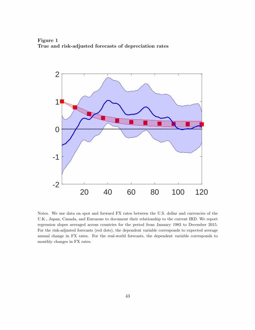
Figure 1True and risk-adjusted forecasts of depreciation rates

20 40 60 80 100 120-2

-1

0

1

2

Notes. We use data on spot and forward FX rates between the U.S. dollar and currencies of the

U.K., Japan, Canada, and Eurozone to document their relationship to the current IRD. We report

regression slopes averaged across countries for the period from January 1983 to December 2015.

For the risk-adjusted forecasts (red dots), the dependent variable corresponds to expected average

annual change in FX rates. For the real-world forecasts, the dependent variable corresponds to

monthly changes in FX rates.

43

Figure 2True and risk-adjusted forecasts of depreciation rates in a simple U.K.model

20 40 60 80 100 120

-1.5

-1

-0.5

0

0.5

1

20 40 60 80 100 120

-1.5

-1

-0.5

0

0.5

1

Notes. We explore variations in the multihorizon pattern in the UIP regressions implied by a simple

bilateral VECM model of U.S. and U.K. On the left panel variations are associated with variations

in the values of elements of αf . VAR corresponds to all αf = 0. On the right panel, we consider

various scenarios of the values of α∗f . The red line with crosses, αf 6= 0, is the same across the two

panels and represents the implications of the estimated VECM.

44

Figure 3True and risk-adjusted cross-covariances of depreciation rates and theinterest rate differential

20 40 60 80 100 120-2

-1

0

1

2

Notes. We report multi-horizon UIP regression patterns in the data (blue line) and in the model

(black line) as cross-country average regression slopes. For the risk-adjusted forecasts (red dots), the

dependent variable corresponds to expected average annual change in FX rates. For the real-world

forecasts, the dependent variable corresponds to monthly changes in FX rates.

45

Figure 4True and risk-adjusted cross-covariances of depreciation rates and thereal exchange rate

20 40 60 80 100 120-0.04

-0.03

-0.02

-0.01

0

0.01

Notes. We report multi-horizon patterns of regressing future nominal depreciation rates on the cur-

rent real exchange rate in the data (blue line) and in the model (black line) as cross-country average

regression slopes. For the risk-adjusted forecasts (red dots), the dependent variable corresponds to

expected average annual change in FX rates. For the real-world forecasts, the dependent variable

corresponds to monthly changes in FX rates.

46

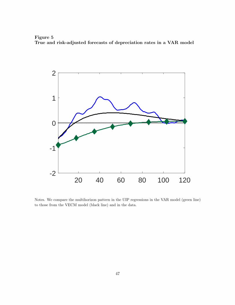
Figure 5True and risk-adjusted forecasts of depreciation rates in a VAR model

20 40 60 80 100 120-2

-1

0

1

2

Notes. We compare the multihorizon pattern in the UIP regressions in the VAR model (green line)

to those from the VECM model (black line) and in the data.

47

Figure 6Long-run UIP in the VECM and VAR models

20 40 60 80 100 120-3

-2

-1

0

1

2

3

Notes. We compare the multihorizon pattern in the long-run UIP regressions in the VAR model

(green line) to those from the VECM model (black line) and in the data (red squares).

48

Figure 7Term structure of nominal and UIP-based risk premiums

1985 1990 1995 2000 2005 2010 2015

-10

0

10

20

Sim

ple

-10

0

10

20

Nom

inal

United Kingdom

1985 1990 1995 2000 2005 2010 2015

0

5

10

0

5

10

United Kingdom

1985 1990 1995 2000 2005 2010 2015

0

2

4

6

0

2

4

6

United Kingdom

1985 1990 1995 2000 2005 2010 2015-10

-5

0

5

10

-10

-5

0

5

10Canada

1985 1990 1995 2000 2005 2010 2015

-2

-1

0

1

2

3

4

5

-2

-1

0

1

2

3

4

5

Canada

1985 1990 1995 2000 2005 2010 2015

-1

0

1

2

3

4

-1

0

1

2

3

4

Canada

1985 1990 1995 2000 2005 2010 2015

-15

-10

-5

0

5

10

15

20

-15

-10

-5

0

5

10

15

20

Euro

1985 1990 1995 2000 2005 2010 2015

-5

0

5

10

-5

0

5

10Euro

1985 1990 1995 2000 2005 2010 2015

-4

-2

0

2

4

6

-4

-2

0

2

4

6Euro

1985 1990 1995 2000 2005 2010 2015-20

-10

0

10

20

-20

-10

0

10

20

Japan

1985 1990 1995 2000 2005 2010 2015

-10

-5

0

5

10

-10

-5

0

5

10

Japan

1985 1990 1995 2000 2005 2010 2015

-10

-5

0

5

-10

-5

0

5

Japan

Notes. The blue line shows the nominal currency risk premium, rpsnt , for horizons n = 1, 12, and 24

months. The black line shows the projection of this premium on the IRD, ∆c`t.

49

Table 1: Posterior mean and stand. dev. of a two country model with the U.S.-U.K.

xt ∆st ∆cπt `t y120,12t ct ∆c`t ∆cy

120,12t ∆c`

12,1t et

µx × 1200 Φx

∆st -0.224 0.065 0.060 -0.792 -2.968 -2.187 -3.430 -0.179 -3.755 -0.053(0.558) (0.049) (0.184) (0.908) (2.059) (3.166) (1.571) (2.319) (3.049) (0.015)

∆cπt -0.224 0.019 0.210 -0.117 -0.067 0.899 1.095 0.510 1.959 0.008(0.558) (0.008) (0.046) (0.163) (0.368) (0.584) (0.295) (0.416) (0.584) (0.003)

`t 4.407 6.06e-04 0.006 0.991 -0.057 -0.153 0.023 -0.022 0.103 1.44e-04(0.663) (7.64e-04) (0.005) (0.015) (0.033) (0.053) (0.026) (0.037) (0.052) (2.62e-04)

y120,12t 1.686 4.56e-05 -9.87e-05 -0.017 0.928 -0.009 -0.025 0.004 -0.020 -3.42e-04

(0.271) (3.50e-04) (0.002) (0.007) (0.016) (0.028) (0.013) (0.018) (0.027) (1.25e-04)ct 0.648 8.12e-05 -0.005 0.065 0.027 0.537 0.028 0.027 0.050 4.75e-04

(0.099) (5.46e-04) (0.003) (0.011) (0.025) (0.041) (0.020) (0.028) (0.039) (1.93e-04)∆c`t -1.726 0.001 -7.72e-04 -0.031 0.019 -0.012 1.032 -0.132 0.582 0.001

(0.396) (8.99e-04) (0.006) (0.016) (0.037) (0.056) (0.028) (0.041) (0.055) (3.01e-04)

∆cy120,12t 0.983 3.12e-04 0.003 0.002 -0.027 0.010 -0.009 0.972 -0.037 -2.61e-04

(0.255) (4.18e-04) (0.003) (0.008) (0.019) (0.031) (0.015) (0.021) (0.030) (1.47e-04)

∆c`12,1t 0.353 -0.001 0.003 0.027 0.011 -0.018 -0.070 0.072 0.468 -6.71e-04

(0.107) (7.08e-04) (0.004) (0.013) (0.030) (0.046) (0.023) (0.033) (0.045) (2.39e-04)et 0.462† 0.045 -0.150 -0.674 -2.900 -3.086 -4.524 -0.689 -5.714 0.939

(0.031) (0.050) (0.188) (0.914) (2.072) (3.196) (1.584) (2.333) (3.076) (0.015)

xt δc,x Σx ×√

12× 100

∆st 0.003 10.115 0 0 0 0 0 0 0(0.001) (0.370) (—) (—) (—) (—) (—) (—) (—)

∆cπt -0.010 0.111 1.674 0 0 0 0 0 0(0.004) (0.086) (0.064) (—) (—) (—) (—) (—) (—)

`t 0.071 -0.014 0.001 0.151 0 0 0 0 0(0.017) (0.007) (0.007) (0.005) (—) (—) (—) (—) (—)

y120,12t 0.084 -0.001 0.004 6.28e-04 0.069 0 0 0 0

(0.034) (0.003) (0.004) (0.003) (0.002) (—) (—) (—) (—)ct -0.504 0.004 -0.018 0.041 0.007 0.098 0 0 0

(0.070) (0.006) (0.006) (0.005) (0.005) (0.003) (—) (—) (—)ct 0.083 0.007 -0.007 0.012 -0.018 0.020 0.172 0 0

(0.026) (0.009) (0.009) (0.009) (0.008) (0.008) (0.006) (—) (—)

∆cy120,12t -0.119 0.005 0.011 -2.04e-04 0.032 0.001 -0.031 0.068 0

(0.035) (0.004) (0.004) (0.004) (0.004) (0.004) (0.004) (0.002) (—)

∆c`12,1t 0.181 -0.018 -0.005 -0.014 -0.001 -0.009 -0.097 -0.047 0.080

(0.054) (0.007) (0.007) (0.008) (0.007) (0.007) (0.006) (0.004) (0.003)et 5.51e-04 10.004 -1.674 0 0 0 0 0 0

(1.87e-04) (0.376) (0.064) (—) (—) (—) (—) (—) (—)

xt µ∗x × 1200 Φ∗x

∆st -3.546 0 0 0 0 0 1 0 0 0(2.771) (—) (—) (—) (—) (—) (—) (—) (—) (—)

∆cπt -3.546 0.035 0.587 0.336 -0.807 0.632 3.024 -0.714 4.503 0.016(2.771) (0.023) (0.036) (0.211) (0.487) (0.558) (0.392) (0.580) (0.599) (0.002)

`t 20.235 5.75e-04 -0.009 1.023 0.059 -0.177 0.089 -0.035 0.176 3.40e-04(1.313) (4.40e-04) (0.001) (0.006) (0.014) (0.026) (0.012) (0.015) (0.025) (7.74e-05)

y120,12t -0.620 3.35e-05 0.001 -0.004 0.972 -0.047 -0.009 7.32e-04 -0.018 -8.40e-05

(0.040) (4.24e-05) (1.60e-04) (0.001) (0.002) (0.004) (0.002) (0.002) (0.003) (9.89e-06)ct 0.525 8.18e-04 -0.008 0.032 0.054 0.460 0.094 -0.040 0.194 1.04e-04

(0.391) (5.98e-04) (0.002) (0.007) (0.017) (0.030) (0.017) (0.017) (0.030) (1.02e-04)∆c`t -3.034 0.001 -0.002 0.005 -0.003 -0.033 1.023 -0.078 0.489 1.16e-04

(2.770) (4.39e-04) (9.03e-04) (0.002) (0.005) (0.016) (0.006) (0.007) (0.018) (3.16e-05)

∆cy120,12t 0.249 2.73e-04 -8.13e-04 0.007 0.011 -0.117 0.018 0.992 -0.072 1.63e-05

(0.067) (1.09e-04) (2.99e-04) (0.001) (0.003) (0.005) (0.002) (0.004) (0.005) (1.74e-05)

∆c`12,1t 0.009 -0.001 0.002 -0.005 0.004 0.031 -0.025 0.097 0.613 -1.31e-04

(0.006) (4.49e-04) (9.60e-04) (0.002) (0.006) (0.017) (0.007) (0.007) (0.019) (3.44e-05)et 0.126† -0.035 -0.587 -0.336 0.807 -0.632 -2.024 0.714 -4.503 0.984

(0.375) (0.023) (0.036) (0.211) (0.487) (0.558) (0.392) (0.580) (0.599) (0.002)

Posterior mean and standard deviation for a two country model of the U.S. and United Kingdom. We reportunconditional means µ∗x, µx, autocovariances matrices Φ∗x,Φx, scale matrix Σx and the vector of loadingsδc,x. The symbol † indicates that the unconditional means of the real exchange rates are not multiplied by1200 (annualization and conversion to percent is not applicable).

50

Table 2: Posterior mean and stand. dev. of a two country model with the U.S.-Canada

xt ∆st ∆cπt `t y120,12t ct ∆c`t ∆cy

120,12t ∆c`

12,1t et

µx × 1200 Φx

∆st 0.212 -0.061 -0.006 -0.529 -1.426 0.345 -2.103 -0.676 -2.456 -0.016(0.266) (0.050) (0.187) (0.733) (1.553) (2.620) (1.622) (2.362) (2.667) (0.008)

∆cπt 0.212 0.029 0.001 -0.142 -0.412 -0.445 -0.671 -1.281 -0.788 0.002(0.266) (0.008) (0.043) (0.119) (0.246) (0.413) (0.265) (0.389) (0.441) (0.001)

`t 4.452 2.76e-04 0.002 0.975 -0.081 -0.107 -0.042 -0.056 -0.022 8.33e-05(0.699) (0.001) (0.007) (0.015) (0.032) (0.052) (0.034) (0.048) (0.056) (1.92e-04)

y120,12t 1.656 9.50e-04 0.004 -0.020 0.936 0.009 -0.042 -0.036 0.017 -3.55e-05

(0.264) (4.92e-04) (0.003) (0.008) (0.016) (0.029) (0.018) (0.027) (0.030) (9.04e-05)ct 0.654 2.89e-04 9.65e-04 0.074 0.021 0.525 0.061 0.092 0.038 1.46e-04

(0.101) (7.69e-04) (0.005) (0.012) (0.025) (0.042) (0.028) (0.040) (0.045) (1.45e-04)∆c`t -0.825 8.57e-04 -0.001 -0.053 -0.034 0.040 0.881 -0.266 0.366 -1.22e-04

(0.369) (0.001) (0.007) (0.017) (0.034) (0.054) (0.033) (0.050) (0.053) (1.97e-04)

∆cy120,12t 0.496 3.34e-04 0.001 -0.008 -0.021 0.013 0.001 0.949 5.23e-04 1.40e-04

(0.204) (5.82e-04) (0.004) (0.010) (0.019) (0.033) (0.021) (0.031) (0.033) (1.06e-04)

∆c`12,1t 0.065 -0.002 0.003 0.027 0.014 -0.017 -0.007 0.148 0.488 3.33e-05

(0.077) (8.93e-04) (0.006) (0.015) (0.028) (0.047) (0.029) (0.043) (0.046) (1.66e-04)et −0.171† -0.090 -0.008 -0.387 -1.014 0.790 -1.431 0.605 -1.669 0.982

(0.043) (0.051) (0.192) (0.741) (1.569) (2.650) (1.644) (2.392) (2.703) (0.008)

xt δc,x Σx ×√

12× 100

∆st 3.15e-04 7.249 0 0 0 0 0 0 0(0.004) (0.262) (—) (—) (—) (—) (—) (—) (—)

∆cπt -0.003 0.009 1.062 0 0 0 0 0 0(0.014) (0.055) (0.039) (—) (—) (—) (—) (—) (—)

`t 0.020 -0.002 -0.003 0.148 0 0 0 0 0(0.049) (0.007) (0.007) (0.004) (—) (—) (—) (—) (—)

y120,12t -0.008 -0.001 0.010 -0.002 0.068 0 0 0 0

(0.037) (0.003) (0.003) (0.003) (0.002) (—) (—) (—) (—)ct 0.248 -0.008 -0.003 0.039 0.006 0.100 0 0 0

(0.155) (0.006) (0.005) (0.005) (0.005) (0.004) (—) (—) (—)∆c`t -0.070 0.016 0.007 0.030 -0.002 0.025 0.141 0 0

(0.029) (0.008) (0.008) (0.013) (0.008) (0.008) (0.005) (—) (—)

∆cy120,12t -0.016 -0.006 3.02e-04 0.021 0.034 0.002 -0.038 0.058 0

(0.050) (0.004) (0.004) (0.007) (0.004) (0.004) (0.003) (0.002) (—)

∆c`12,1t -0.281 -0.010 -0.008 -0.039 -0.010 -0.021 -0.072 -0.047 0.074

(0.072) (0.006) (0.007) (0.011) (0.007) (0.007) (0.005) (0.004) (0.003)et 1.99e-04 7.240 -1.062 0 0 0 0 0 0

(9.72e-05) (0.267) (0.039) (—) (—) (—) (—) (—) (—)

xt µ∗x × 1200 Φ∗x

∆st 24.581 0 0 0 0 0 1 0 0 0(3.139) (—) (—) (—) (—) (—) (—) (—) (—) (—)

∆cπt 24.581 0.067 0.158 1.913 -2.807 0.557 -1.457 -2.819 -1.241 0.006(3.139) (0.033) (0.039) (0.351) (0.640) (0.255) (0.285) (0.656) (0.601) (8.01e-04)

`t 22.181 -2.13e-04 -0.006 1.018 0.040 -0.008 -0.008 -0.019 -0.008 4.03e-05(1.232) (6.88e-04) (0.003) (0.008) (0.012) (0.006) (0.005) (0.013) (0.010) (2.38e-05)

y120,12t -0.524 4.51e-05 4.59e-04 7.41e-04 0.977 -0.073 0.011 0.018 0.009 -7.04e-06

(0.030) (5.73e-05) (2.78e-04) (8.82e-04) (0.002) (7.27e-04) (0.002) (0.003) (0.002) (3.36e-06)ct 4.898 2.33e-04 -0.020 0.095 0.039 0.395 0.055 0.062 0.050 1.12e-04

(0.890) (8.70e-04) (0.003) (0.013) (0.021) (0.026) (0.016) (0.030) (0.030) (3.20e-05)∆c`t 24.844 8.20e-04 1.00e-03 -0.008 0.010 0.032 0.999 -0.094 0.461 -2.41e-05

(3.138) (6.21e-04) (0.001) (0.005) (0.005) (0.019) (0.002) (0.008) (0.019) (1.16e-05)

∆cy120,12t 0.182 5.47e-05 -1.68e-04 0.005 0.010 -0.057 0.008 1.005 -0.106 -5.45e-06

(0.065) (2.87e-04) (0.001) (0.004) (0.003) (0.012) (0.002) (0.004) (0.005) (7.57e-06)

∆c`12,1t 0.009 -8.37e-04 -9.71e-04 0.009 -0.012 -0.035 6.11e-04 0.117 0.642 2.79e-05

(0.004) (6.37e-04) (0.001) (0.005) (0.005) (0.020) (0.002) (0.009) (0.020) (1.22e-05)et −0.168† -0.067 -0.158 -1.913 2.807 -0.557 2.457 2.819 1.241 0.994

(0.435) (0.033) (0.039) (0.351) (0.640) (0.255) (0.285) (0.656) (0.601) (8.01e-04)

Posterior mean and standard deviation for a two country model of the U.S. and Canada. We reportunconditional means µ∗x, µx, autocovariances matrices Φ∗x,Φx, scale matrix Σx and the vector of loadingsδc,x. The symbol † indicates that the unconditional means of the real exchange rates are not multiplied by1200 (annualization and conversion to percent is not applicable).

51

Table 3: Posterior mean and stand. dev. of a two country model with the U.S.-Euro

xt ∆st ∆cπt `t y120,12t ct ∆c`t ∆cy

120,12t ∆c`

12,1t et

µx × 1200 Φx

∆st 0.917 0.133 0.097 0.039 1.640 3.423 -4.143 -3.786 -8.059 -0.037(0.330) (0.049) (0.191) (0.840) (2.194) (3.151) (1.583) (2.537) (2.844) (0.011)

∆cπt 0.917 0.022 0.103 0.248 0.128 -1.303 0.585 0.473 -0.186 0.003(0.330) (0.007) (0.044) (0.132) (0.365) (0.539) (0.261) (0.435) (0.455) (0.002)

`t 4.391 1.74e-04 0.006 0.981 -0.059 -0.138 0.035 -0.001 0.109 4.94e-05(0.624) (7.69e-04) (0.005) (0.013) (0.035) (0.052) (0.026) (0.042) (0.046) (1.79e-04)

y120,12t 1.651 -3.33e-05 -6.93e-04 5.56e-05 0.974 0.020 -0.084 -0.087 -0.121 -4.38e-04

(0.211) (3.48e-04) (0.003) (0.007) (0.018) (0.027) (0.014) (0.022) (0.024) (8.62e-05)ct 0.651 4.01e-04 0.004 0.054 0.010 0.536 0.048 0.054 0.017 3.26e-04

(0.094) (5.53e-04) (0.004) (0.010) (0.027) (0.041) (0.021) (0.033) (0.036) (1.35e-04)∆c`t 0.651 0.001 0.014 -0.011 0.034 0.039 0.959 -0.251 0.698 -1.05e-04

(0.435) (0.001) (0.007) (0.017) (0.043) (0.060) (0.030) (0.048) (0.055) (2.35e-04)

∆cy120,12t 0.397 -8.58e-05 0.004 0.007 -0.011 -0.011 -0.056 0.927 -0.097 -2.77e-04

(0.272) (4.35e-04) (0.003) (0.008) (0.022) (0.033) (0.017) (0.027) (0.029) (1.06e-04)

∆c`12,1t 0.149 -0.002 -0.009 -0.003 0.027 0.020 -0.012 0.117 0.375 -9.71e-06

(0.080) (8.59e-04) (0.006) (0.015) (0.037) (0.052) (0.026) (0.042) (0.047) (1.96e-04)et 0.221† 0.111 -0.006 -0.209 1.513 4.726 -4.728 -4.259 -7.872 0.960

(0.042) (0.049) (0.195) (0.848) (2.217) (3.187) (1.600) (2.565) (2.869) (0.011)

xt δc,x Σx ×√

12× 100

∆st -5.63e-04 9.777 0 0 0 0 0 0 0(0.003) (0.352) (—) (—) (—) (—) (—) (—) (—)

∆cπt -0.019 0.031 1.347 0 0 0 0 0 0(0.003) (0.069) (0.049) (—) (—) (—) (—) (—) (—)

`t 0.113 0.003 -8.41e-04 0.149 0 0 0 0 0(0.016) (0.007) (0.007) (0.005) (—) (—) (—) (—) (—)

y120,12t 0.158 -0.002 -0.001 0.005 0.067 0 0 0 0

(0.032) (0.003) (0.003) (0.003) (0.002) (—) (—) (—) (—)ct 0.261 0.008 -0.004 0.038 0.008 0.099 0 0 0

(0.105) (0.005) (0.005) (0.005) (0.005) (0.004) (—) (—) (—)∆c`t -0.185 4.36e-04 -0.005 0.092 0.002 0.004 0.176 0 0

(0.016) (0.010) (0.010) (0.013) (0.009) (0.009) (0.007) (—) (—)

∆cy120,12t -0.291 -0.007 -4.11e-04 -0.013 0.060 9.02e-04 -0.004 0.056 0

(0.049) (0.004) (0.004) (0.004) (0.003) (0.003) (0.003) (0.002) (—)

∆c`12,1t 0.323 -0.012 0.008 -0.023 -0.006 -0.010 -0.144 -0.015 0.068

(0.114) (0.008) (0.008) (0.011) (0.008) (0.008) (0.007) (0.004) (0.002)et -1.49e-04 9.746 -1.347 0 0 0 0 0 0

(3.90e-05) (0.356) (0.049) (—) (—) (—) (—) (—) (—)

xt µ∗x × 1200 Φ∗x

∆st 9.658 0 0 0 0 0 1 0 0 0(1.394) (—) (—) (—) (—) (—) (—) (—) (—) (—)

∆cπt 9.658 -0.068 0.315 3.581 0.095 -0.308 1.144 1.757 -1.271 0.004(1.394) (0.028) (0.038) (0.453) (0.936) (0.811) (0.207) (0.683) (0.631) (3.77e-04)

`t 20.695 -2.14e-04 0.007 0.968 0.064 -0.041 -0.017 -0.062 0.125 -2.69e-05(0.989) (4.51e-04) (0.001) (0.009) (0.011) (0.025) (0.003) (0.012) (0.025) (1.11e-05)

y120,12t -0.634 6.30e-05 -7.50e-04 -0.001 0.973 -0.068 -0.002 0.007 -0.017 2.02e-05

(0.036) (4.31e-05) (1.23e-04) (0.001) (0.002) (0.003) (0.001) (0.003) (0.004) (2.66e-06)ct 0.175 -0.002 0.004 -0.024 0.061 0.535 -0.033 -0.038 0.064 8.26e-05

(0.325) (6.03e-04) (7.27e-04) (0.010) (0.018) (0.024) (0.009) (0.021) (0.029) (1.69e-05)∆c`t 10.137 5.29e-04 1.30e-05 0.011 0.023 -0.069 0.983 -0.163 0.660 3.05e-05

(1.394) (4.44e-04) (2.60e-04) (0.002) (0.007) (0.023) (0.002) (0.012) (0.026) (5.24e-06)

∆cy120,12t -0.324 -3.14e-05 -0.001 0.008 0.012 -0.058 -0.005 0.976 -0.054 2.23e-05

(0.045) (2.55e-04) (2.17e-04) (0.001) (0.003) (0.008) (0.001) (0.004) (0.009) (2.73e-06)

∆c`12,1t -0.004 -5.36e-04 -6.23e-05 -0.012 -0.025 0.069 0.019 0.188 0.437 -3.27e-05

(0.004) (4.48e-04) (2.68e-04) (0.002) (0.008) (0.023) (0.002) (0.012) (0.026) (5.47e-06)et 0.438† 0.068 -0.315 -3.581 -0.095 0.308 -0.144 -1.757 1.271 0.996

(0.411) (0.028) (0.038) (0.453) (0.936) (0.811) (0.207) (0.683) (0.631) (3.77e-04)

Posterior mean and standard deviation for a two country model of the U.S. and Euro. We reportunconditional means µ∗x, µx, autocovariances matrices Φ∗x,Φx, scale matrix Σx and the vector of loadingsδc,x. The symbol † indicates that the unconditional means of the real exchange rates are not multiplied by1200 (annualization and conversion to percent is not applicable).

52

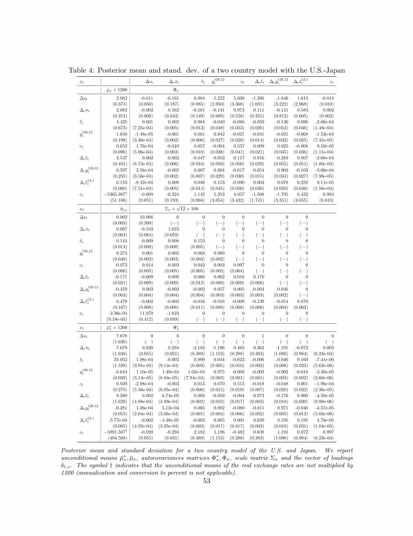
Table 4: Posterior mean and stand. dev. of a two country model with the U.S.-Japan

xt ∆st ∆cπt `t y120,12t ct ∆c`t ∆cy

120,12t ∆c`

12,1t et

µx × 1200 Φx

∆st 2.082 -0.011 -0.161 0.984 5.222 5.030 -1.396 -1.846 1.014 -0.014(0.374) (0.050) (0.187) (0.885) (2.950) (3.368) (1.691) (3.222) (2.968) (0.010)

∆cπt 2.082 -0.002 0.162 -0.161 -0.131 0.973 0.111 -0.141 0.583 0.002(0.374) (0.008) (0.043) (0.149) (0.689) (0.558) (0.355) (0.812) (0.605) (0.002)

`t 4.425 0.001 0.002 0.984 -0.040 -0.088 -0.059 -0.136 0.096 -2.66e-04(0.673) (7.25e-04) (0.005) (0.013) (0.048) (0.053) (0.026) (0.054) (0.046) (1.48e-04)

y120,12t 1.650 -1.48e-05 -0.001 0.001 0.942 -0.021 -0.041 -0.021 -0.068 -1.53e-04

(0.199) (3.30e-04) (0.002) (0.006) (0.027) (0.028) (0.014) (0.032) (0.025) (7.45e-05)ct 0.652 1.76e-04 -0.010 0.057 -0.004 0.557 0.009 0.025 -0.008 9.10e-05

(0.096) (5.06e-04) (0.003) (0.010) (0.038) (0.041) (0.021) (0.045) (0.036) (1.11e-04)∆c`t 2.547 0.002 -0.002 -0.047 -0.053 0.117 0.916 -0.283 0.807 -2.68e-04

(0.401) (8.74e-04) (0.006) (0.016) (0.050) (0.056) (0.029) (0.055) (0.051) (1.80e-04)

∆cy120,12t 0.597 2.58e-04 -0.002 0.007 0.004 -0.017 -0.054 0.903 -0.103 -3.06e-04

(0.235) (3.56e-04) (0.002) (0.007) (0.029) (0.030) (0.015) (0.034) (0.027) (7.98e-05)

∆c`12,1t 0.153 -8.42e-04 0.008 0.046 0.153 -0.090 0.003 0.078 0.258 9.11e-05

(0.060) (7.51e-04) (0.005) (0.014) (0.045) (0.050) (0.026) (0.050) (0.046) (1.56e-04)et −5365.387† -0.009 -0.324 1.145 5.353 4.057 -1.508 -1.705 0.432 0.983

(51.106) (0.051) (0.193) (0.904) (3.054) (3.432) (1.741) (3.351) (3.055) (0.010)

xt δc,x Σx ×√

12× 100

∆st 0.002 10.966 0 0 0 0 0 0 0(0.003) (0.399) (—) (—) (—) (—) (—) (—) (—)

∆cπt 0.007 -0.103 1.623 0 0 0 0 0 0(0.004) (0.084) (0.059) (—) (—) (—) (—) (—) (—)

`t 0.144 -0.009 0.008 0.153 0 0 0 0 0(0.014) (0.008) (0.008) (0.005) (—) (—) (—) (—) (—)

y120,12t 0.274 0.001 0.002 0.003 0.069 0 0 0 0

(0.048) (0.003) (0.003) (0.003) (0.002) (—) (—) (—) (—)ct -0.073 0.014 0.003 0.042 0.003 0.097 0 0 0

(0.080) (0.005) (0.005) (0.005) (0.005) (0.004) (—) (—) (—)∆c`t -0.171 -0.009 0.009 0.066 0.002 0.016 0.170 0 0

(0.021) (0.009) (0.009) (0.012) (0.009) (0.009) (0.006) (—) (—)

∆cy120,12t -0.459 0.003 -0.002 -0.002 0.057 0.005 -0.003 0.046 0

(0.063) (0.004) (0.004) (0.004) (0.003) (0.003) (0.003) (0.002) (—)

∆c`12,1t 0.478 -0.002 -0.003 -0.016 -0.016 -0.009 -0.139 -0.014 0.070

(0.167) (0.008) (0.008) (0.011) (0.008) (0.008) (0.006) (0.004) (0.003)et -2.36e-04 11.070 -1.623 0 0 0 0 0 0

(9.18e-05) (0.412) (0.059) (—) (—) (—) (—) (—) (—)

xt µ∗x × 1200 Φ∗x

∆st 7.678 0 0 0 0 0 1 0 0 0(1.630) (—) (—) (—) (—) (—) (—) (—) (—) (—)

∆cπt 7.678 0.020 0.294 -2.182 -1.196 0.482 0.362 -1.191 -0.072 0.003(1.630) (0.055) (0.031) (0.389) (1.153) (0.288) (0.383) (1.086) (0.984) (6.23e-04)

`t 25.052 1.98e-04 -0.002 0.999 0.044 -0.023 -0.006 -0.046 0.169 -7.41e-06(1.528) (3.91e-04) (9.14e-04) (0.003) (0.005) (0.010) (0.002) (0.008) (0.023) (5.62e-06)

y120,12t -0.644 1.10e-05 1.49e-04 1.02e-04 0.975 -0.069 -0.003 -0.002 -0.018 -3.30e-05

(0.039) (3.14e-05) (8.94e-05) (7.94e-04) (0.003) (0.001) (0.001) (0.003) (0.002) (3.60e-06)ct 0.939 -2.98e-04 -0.003 0.013 0.070 0.513 -0.018 -0.048 0.001 -1.96e-04

(0.275) (5.56e-04) (6.95e-04) (0.006) (0.015) (0.019) (0.007) (0.020) (0.032) (2.36e-05)∆c`t 8.280 0.002 6.74e-05 0.002 -0.059 -0.004 0.973 -0.176 0.900 -4.50e-05

(1.629) (4.88e-04) (3.89e-04) (0.002) (0.010) (0.017) (0.003) (0.010) (0.030) (9.99e-06)

∆cy120,12t -0.281 1.36e-04 5.12e-04 0.005 0.002 -0.080 -0.011 0.971 -0.046 -4.57e-05

(0.055) (2.04e-04) (3.06e-04) (0.001) (0.004) (0.006) (0.002) (0.005) (0.013) (5.03e-06)

∆c`12,1t -5.77e-04 -0.002 -4.38e-05 -0.002 0.065 0.001 0.029 0.195 0.195 4.78e-05

(0.005) (4.92e-04) (3.95e-04) (0.002) (0.011) (0.017) (0.003) (0.010) (0.031) (1.04e-05)et −5891.507† -0.020 -0.294 2.182 1.196 -0.482 0.638 1.191 0.072 0.997

(494.508) (0.055) (0.031) (0.389) (1.153) (0.288) (0.383) (1.086) (0.984) (6.23e-04)

Posterior mean and standard deviation for a two country model of the U.S. and Japan. We reportunconditional means µ∗x, µx, autocovariances matrices Φ∗x,Φx, scale matrix Σx and the vector of loadingsδc,x. The symbol † indicates that the unconditional means of the real exchange rates are not multiplied by1200 (annualization and conversion to percent is not applicable).

53

Table 5: Pricing errors across countries

U.K. CAN EURO JPN

`1t − `3t + 3 0.045 0.049 0.048 0.058

`1t − `6t + 6 0.035 0.035 0.038 0.040y3t 0.061 0.049 0.052 0.045

y12t 0.113 0.109 0.097 0.098y24t 0.150 0.146 0.132 0.139y36t 0.160 0.157 0.142 0.151y48t 0.158 0.155 0.140 0.149y60t 0.150 0.148 0.132 0.141y84t 0.131 0.129 0.115 0.120y3t 0.109 - - -

y24t 0.155 0.154 0.146 0.130y36t 0.165 0.155 0.152 0.142y48t 0.163 0.150 0.150 0.151y60t 0.155 0.145 0.145 0.154y84t 0.138 0.138 0.134 0.151

y120t 0.118 0.128 0.122 0.125

Posterior mean estimates of the pricing errors in annualized percentage points, 100√

diag(ΣyΣ′y

)× 12, for

the U.K., Canada, Euro, and Japan. These are reported for yields of different maturity that enter Y(2)t .

54

Table 6: Estimates of the speed of mean reversion coefficients

U.K. CAN EURO JPNαf α∗f αf α∗f αf α∗f αf α∗f

∆st -0.261 0 -0.130 0 -0.272 0 -0.097 0(0.180) (—) (0.156) (—) (0.209) (—) (0.092) (—)

∆cπt 0.218 0.432 0.146 0.323 0.155 0.207 0.100 0.212(0.144) (0.232) (0.162) (0.297) (0.147) (0.139) (0.105) (0.118)

`t 0.006 0.014 0.005 0.002 0.003 -0.002 -0.020 1.38e-04(0.012) (0.006) (0.013) (0.001) (0.013) (0.001) (0.014) (5.94e-05)

y120,12t -0.042 -0.011 -0.006 -5.80e-04 -0.082 0.003 -0.032 -0.007

(0.022) (0.004) (0.017) (3.54e-04) (0.046) (0.002) (0.019) (0.003)ct 0.115 0.003 0.044 0.036 0.120 0.027 0.038 -0.080

(0.066) (0.001) (0.058) (0.023) (0.082) (0.014) (0.052) (0.032)∆c`t 0.072 0.009 -0.012 -0.004 -0.008 0.002 -0.029 -0.004

(0.033) (0.003) (0.023) (0.002) (0.021) (8.84e-04) (0.025) (0.002)

∆cy120,12t -0.032 0.002 0.027 -7.28e-04 -0.042 0.003 -0.054 -0.008

(0.022) (6.42e-04) (0.023) (3.53e-04) (0.028) (0.002) (0.021) (0.003)

∆c`12,1t -0.145 -0.030 0.009 0.013 -0.006 -0.008 0.039 0.017

(0.087) (0.013) (0.067) (0.008) (0.075) (0.005) (0.077) (0.008)

Posterior mean and standard deviation estimates of α and α∗ for the U.K., Canada, Euro, and Japan. Thefactors have been re-scaled to have unit variance.

Table 7: Log-predictive scores for VECM and VAR models across countries

U.K. CAN EURO JPN

VAR -183.59 -166.88 -175.92 -170.23VECM -183.99 -169.28 -175.98 -170.12

Log-predictive scores for the U.K., Canada, Euro, and Japan for the VECM and VAR models.

LPS = −T−1∑Tt=1 p

(yt|y1:t−1; θ

)where θ is the posterior median. Lower values of the LPS are preferred.

55