Multidimensional Measurement of Poverty in Sub … · Multidimensional Measurement of Poverty in...

Batana Working Paper No.13

Multidimensional Measurement of Poverty inSub-Saharan Africa ∗

Yélé Maweki Batana †

Abstract

Since the seminal works of Sen, poverty is recognized as multidimensional phe-nomenon. Recently, there is a renewed interest in this approach since relevantdatabases became available. Several methods of aggregation have been suggestedto measure poverty in this way. Up to now, there is no consensus on the best mea-sure. However, a suitable measure should satisfy some useful properties. Alkireand Foster (2007) propose a multidimensional poverty measure using a counting ap-proach. This method is applied to estimate multidimensional poverty in fourteen Sub-Saharan African countries. Poverty identification is based on four dimensions (assets,health, schooling and empowerment). The main results show important differences inpoverty among the countries of the sample. The findings are compared with some stan-dard measures such as Human Development indicators (HDI) and the income povertyamong others. Comparisons show that consider additional dimensions leads to coun-try rankings different from the standard-based rankings. Poverty is also decomposedby rural and urban location and by dimension. Rural areas are identified obviously asthe poorest while schooling appear to be in general the most contributor in poverty.Finally, some robustness and sensitivity analyses are done.

Keywords: Multidimensional poverty, counting measurement, robustness analysis, Sub-Saharan Africa.

JEL Classification: C12,D31,I31,I32.

OPHI Working Paper 13August, 2008

∗I am grateful for significant comments of Sabina Alkire. I am also grateful for inputs of Ana Lugo, YuJiantuo, Maria Emma Santos, Anna Hiltunen and David Vazquez-Guzman

†OPHI, Queen Elizabeth House, University of Oxford and CIRPÉE, Université Laval; Email:[email protected]

Oxford Poverty & Human Development Initiative, OPHIwww.ophi.org.uk

1


1 Introduction

Fighting extreme poverty and improving health and education are among the mainMillennium Development Goals (MDGs) agreed by 189 heads of state in 2000. To ef-ficiently achieve these goals, it would be helpful to propose a suitable measurement ofpoverty that allows the targeting of priorities. Income poverty measures have been usu-ally used to analyse poverty in developing countries including those from Sub-SaharanAfrica. Several poverty indices2, which follow from the utilitarian definition of wel-fare, are tremendously useful for estimating poverty levels and making inter-temporal andinter-country comparisons. However, some arguments suggest now to go beyond thesemoney-metric measures and consider other poverty measurements. The first argument, amore practical one, relates to the fact that the quality (regularity and comparability) ofincome/expenditures data is often poor in many developing countries, especially in Sub-Saharan African ones which are generally regarded as those showing the most poverty andextreme poverty. A second argument, more theoretical and methodological, concerns themultidimensional nature of well-being. Indeed, since the seminal works of Sen (1976;1985; 1992; 1995), well-being and poverty are now seen as multidimensional phenomena.The well-being of an individual depends thus not only on income, but also on several otherdimensions or capabilities such as health, education, empowerment etc. Nowadays, thereis a renewed interest in the multidimensional approach of poverty since relevant databasesbecome increasingly available to enable comparative analyses3.

Several aggregation methods have been suggested to capture multidimensionalpoverty. Some of these approaches are axiomatic and are extensions of the unidimensionalpoverty indices (Tsui 2002; Atkinson 2003; Bourguignon and Chakravarty 2003). Othernumerous methods, mainly non-axiomatic, are developed in the literature. For example,among others the fuzzy set approach (Cerioli and Zani 1990; Cheli and Lemmi 1994;Chiappero-Martinetti 2006), the distance function method (Lovell, Richardson, Travers,and Wood 1994; Anderson, Crawford, and Liecester 2005; Deutsch and Silber 2005) andthe entropy measures approach (Maasoumi 1993; Deutsch and Silber 2005; Maasoumi andLugo 2008). Other approaches, more centered on statistical methods, were also adoptedsuch as the inertia approach and the factor analysis (Klasen 2000; Sahn and Stifel 2000;Sahn and Stifel 2003a). More recently, some methods from psychometric literature (Struc-tural Equation Model and MIMIC models) have been introduced in the well-being analysis(Wagle 2005; Di Tommaso 2007; Krishnakumar 2007; Krishnakumar and Ballon 2008).

2For instance, Foster, Greer, and Thorbecke (1984) and Watts (1968) indices.3Demography and Health surveys (DHS) in Africa.

www.ophi.org.uk 2


Few studies are carried out to measure multidimensional poverty in Sub-SaharanAfrican countries. Sahn and Stifel (2000) used Demography and Health Surveys (DHS) tocompare poverty through time within and between fifteen African countries. Well-being ismeasured by an asset index estimated from a factor analysis (FA) of various household so-cioeconomic indicators. Booysen, Von Maltitz, Van der Berg, Burger, and Du Rand (2008)extend the work of Sahn and Stifel (2000) by analysing poverty comparisons over time andacross countries, using multiple correspondence analysis (MCA) rather than FA and addingmore recent surveys. By using a household survey from South Africa, Klasen (2000) com-pares the standard expenditure-based poverty measure with a multidimensional deprivationmeasure and find that, although there is a strong correlation between them, this correla-tion decreases when the worst-off of the population are considered. Von Maltzahn andDurrheim (2008) also use different poverty measures and obtain, for instance, that house-hold income levels are correlated with the living standard measure (LSM) scores, meaningthat there is an underlying dimension of poverty common to all measures. Duclos, Sahn,and Younger (2006a) and Batana and Duclos (2008) extend the analysis by integrating thebivariate stochastic dominance analysis. The first applies the methods to two measuresof well-being, namely household expenditures per capita and children’s height-for-age z

scores in three countries, while the second uses an asset index rather than the householdexpenditures for six West African countries.

Up to now, there is no consensus about the best multidimensional poverty measure.For example, which measure could allow better targeting of the poor and suggest moreeffective poverty-reduction policies? One issue a good poverty measure needs to addressis identification. With multidimensional poverty, identification of the poor arises at twostages. The first stage is to identify the deprived individuals in each dimension while thesecond concerns the poverty definition across all dimensions. A measure also needs tosatisfy useful properties such as the decomposability. By enabling decomposability acrossindividuals and across dimensions, the measure is able to guide good policies. Alkire andFoster (2007) propose a counting approach for measuring the multidimensional poverty.This approach is appealing for several reasons. First, it is easy to implement so manypeople could use it. Secondly, it integrates the identification analysis using two cutoffs,where the first is the known dimension-specific threshold for identifying the individualsdeprived in that dimension. The second cutoff is the number of dimensions (or weightedsum) in which an individual has to be deprived to be considered poor. Moreover, thisapproach satisfies several desirable properties including decomposability. One has also thelatitude to assign different weights to each dimension.

The main objective of this paper is to apply the above multidimensional counting

www.ophi.org.uk 3


method to estimate multidimensional poverty in fourteen Sub-Saharan African countries.That is an interesting empirical contribution since the analysis goes beyond the previous onAfrica by taking account simultaneously of additional dimensions such as health, school-ing and empowerment. The main results show important differences in poverty among thecountries of the sample. The findings are further compared with the ones from standardmeasures such as human development indicators (HDI), income poverty, gender relateddevelopment index and asset index. Comparisons show that consider additional dimen-sions leads to country rankings different from the standard-based rankings. Decomposi-tions are done by rural/urban location and by dimension. This enables us to identify ruralareas, obviously, as the poorest and schooling as the most contributor in poverty. Finally,some robustness and sensitivity analyses are performed. The robustness analysis allows re-searchers to check whether the differences in poverty between countries significantly holdfor a full range of between-dimensional cutoffs. The sensitivity analysis concerns the im-plications of possible changes in each dimensional threshold. The analysis undertaken inthis paper seems relevant to capture multidimensional poverty more accurately and couldprovide tools for better poverty-reducing policies.

The paper is structured as follows. Section 2 describes the methodology for estimat-ing the multidimensional poverty and adds some short extensions for doing decompositionand robustness analyses. Empirical applications consisting in data description, poverty es-timation results and comparisons with alternative measures are found in section Section 3.Section 4 analyses the poverty decompositions by urban and rural location and by dimen-sion, while section 5 presents some robustness and sensitivity results. Section 6 concludes.

www.ophi.org.uk 4


2 Methodology

Alkire and Foster (2007) suggest a counting approach which follows the method ofaggregation proposed by Foster, Greer, and Thorbecke (1984) in the sense that it is builton the same family of measures. This family satisfies a certain number of axioms such assymmetry, replication invariance, decomposability, etc.

Consider a population of n individuals. Let d ≥ 2 be the number of dimensions andx = [xij] the n × d matrix of achievements, where xij is the achievement of individual i

(i = 1, ..., n) in dimension j (j = 1, ..., d). x is of the following form:

x =

x11 · x1j · x1d

· · · · ·xi1 · xij · xid

· · · · ·xn1 · xnj · xnd

Let z be a row vector of dimension-specific thresholds zj , xi the row vector of indi-vidual i’s achievements in each dimension, and xj a column vector of dimension j achieve-ments across the set of individuals. The first step for measuring the poverty is to identifywho is poor.

2.1 Identification

For simplicity we assume all dimensions are equally weighted, an assumption we canrelax later. Suppose that a matrix of deprivations x̃0 = [x̃0

ij] is derived from x as follows:

for all i and j, x̃0ij =

{1 if xij < zj

0 otherwise

For example, x̃0ij = 1 means that individual i is deprived in dimension j and x̃0

ij = 0 thatindividual i is not.

By summing each row of x̃0, we obtain a column vector c of deprivation counts con-taining ci the number of deprivations suffered by individual i.

For identifying, consider the identification function ρ(xi; z) such that:

ρ(xi; z) =

{1 if individual i is multidimensionally poor

0 if not(1)

www.ophi.org.uk 5


Let k be the cutoff. An individual i will be considered as poor or ρk(xi; z) = 1 if ci ≥ k.ρk(xi; z) is the identification function relating to the cutoff k. The equation (1) could berewritten:

ρk(xi; z) = I(ci ≥ k) =

{1 if ci ≥ k

0 if not(2)

I(ci ≥ k) is the standard indicator function taking the value 1 if the expression in bracketsholds and the value 0 if not.

The central question here is following: which is the minimum number k of depriva-tions an individual should suffer to be considered poor?

In the multidimensional context, there are two prominent criteria of identification.The first is known as union definition and considers an individual as poor if he or she isdeprived in at least one dimension. In this case, the cutoff k = 1. This definition seems tostrong and could overestimate the poverty, especially when the number of dimensions d ishigh enough with possible substitutability among some dimensions.

A second criterion is the intersection definition which considers an individual as pooronly when he or she is deprived in all the dimensions, i.e. with k = d. This could on theother hand underestimate the poverty by not considering, for example, a healthy homelessas poor when health and housing are two of the dimensions.

A third alternative is to choose an intermediate definition with 1 < k < d. In thecase of only two dimensions, this criterion will be a combination of these dimensions asproposed by Duclos, Sahn, and Younger (2006b). When a cutoff k is retained, the next stepconsists in proposing a suitable poverty measure.

2.2 Multidimensional poverty measure

Let M(x; z) be the class of multidimensional poverty measures suggested by Alkireand Foster (2007). The first measure is given by headcount ratio. Let qk be the number ofpoor identified according to the thresholds vector z and the cutoff k, the headcount ratio H

is following:

H =qk

n, (3)

with qk =n∑

i=1

ρk(xi; z) =n∑

i=1

I(ci ≥ k)

www.ophi.org.uk 6


The share of possible deprivations suffered by a poor individual i is given by:

ci(k) =1

d[ciρk(xi; z)], (4)

and the average deprivation share across the poor by:

A =1

qkd

n∑i=1

ciρk(xi; z). (5)

The second measure proposed by Alkire and Foster (2007) combines H and A toobtain an expression satisfying the dimensional monotonicity (unlike H). The new measureM0 called adjusted headcount ratio is given by:

M0 = HA =1

nd

n∑i=1

ciρk(xi; z). (6)

When some dimensions are represented by cardinal data, it is then possible to derivea class of adjusted FGT measures. In this case, a new matrix x̂1 will be derived fromx̃0 by replacing 1 by the respective normalized gaps g1

ij =(zj−xij)

zjfor all cardinal data j

and for all individuals i. One could also consider the general case for a matrix x̂α, withgα

ij =(zj−xij)

α

zαj

. Consider the following expression of Gα:

Gα =1

n∑i=1

ciρk(xi; z)

d∑j=1

n∑i=1

gαijρk(xi; z),

the adjusted FGT measure Mα = HAGα is finally given by:

Mα =1

nd

d∑j=1

n∑i=1

gαijρk(xi; z). (7)

For α = 0,d∑

j=1

n∑i=1

gαijρk(xi; z) =

n∑i=1

ciρk(xi; z) and we obtain M0.

For α = 1, we obtain the adjusted poverty gap M1.

A useful property satisfied by this measure is decomposability. Suppose that the n-size population is divided for example into two mutually exclusive subgroups of sizes n1

and n2 respectively. It is such a case when one considers urban and rural populations. Thetwo subgroups are respectively represented by two matrices of achievements x1 and x2.Then we have:

M(x; z) =n1

nM(x1; z) +

n2

nM(x2; z). (8)

www.ophi.org.uk 7


This decomposition could be generalized in a straightforward way to any number ofexclusive subgroups.

2.3 Robustness analysis methods

There is no unambiguous way to choose dimensional thresholds (zj) and a uniquecutoff (k) to identify the poor. When we have to compare multidimensional poverty be-tween two or more countries as it is the case in this paper, it may be useful to check thatany ordered relation between them holds for the full range of k and for reasonable variousthreshold vectors z. This analysis, known in the unidimensional poverty context as stochas-tic dominance (Atkinson 1987; Foster and Shorrocks 1988a, 1988b), has been statisticallyapplied to the bidimensional poverty by Duclos, Sahn, and Younger (2006a, 2006b) andBatana and Duclos (2008). Such comparisons are normatively robust since they are provedto be consistent with welfare dominance.

With Alkire and Foster (2007) approach, a straightforward way to make a quite similaranalysis is to consider the range of k. In fact, if d is high enough, it is possible to makerobustness analyses by describing the poverty at each point of the full range ok k = 1, ..., d.Then, comparing the multidimensional poverty in two populations for each k could beregarded as a dominance analysis. An increase in k could correspond to a decrease in thepoverty line for an aggregated dimension derived from factor analysis over all dimensions.Atkinson (2003) suggests such a dominance analysis where the robustness is checked alongthe variation from an union definition of poverty to an intersection definition. Given twodistributions A and B with F and G as respective cumulative distribution functions (cdfs).The first comparison of poverty will be in terms of the headcount ratio. Let nA and nB bethe respective size of A and B. Multidimensional poverty4 is said to be greater in A thanin B, for a given k, if HA > HB. B then dominates A in poverty if the previous conditionholds for all k. Following Davidson and Duclos (2006), these relations could be tested byspecifying the null hypothesis of non dominance as follows:

H0 :1

nA

nA∑i=1

I(cAi ≥ k)− 1

nB

nB∑

l=1

I(cBl ≥ k) ≤ 0 for some k;

versus

H1 :1

nA

nA∑i=1

I(cAi ≥ k)− 1

nB

nB∑

l=1

I(cBl ≥ k) > 0 for all k. (9)

4The dominance analysis here comes down to a simple unidimensional dominance since all dimensionsare aggregated in a vector c of deprivation counts.

www.ophi.org.uk 8


cAi and cB

l are the numbers of deprivations suffered by individuals i and l respec-tively from the distributions A and B. The tests are based on the empirical likelihood ratio(Davidson and Duclos 2006). Given pA

i and pBl the probabilities associated respectively

to the individuals i and l, our statistic is obtained by maximizing the following empiricallikelihood function (ELF ):

maxpA

i ,pBl

∑i

nAi log pA

i +∑

l

nBl log pB

l (10)

subject to∑

i

pAi = 1,

∑

l

pBl = 1

First, the unconstrained and maximized ELF is estimated according to (10). Then, the con-strained maximized ELF is still estimated from (10) by adding a new constraint inducedby the null hypothesis:

nA∑i=1

pAi I(cA

i ≥ k)−nB∑

l=1

pBl I(cB

l ≥ k) = 0 (11)

The test ratio for each k is given by the difference between the two ELFs. If the mini-mum test ratio over the k is great enough, the null will be rejected. To conduct the samedominance analysis for M0, the following constraint will be considered:

nA∑i=1

cAi pA

i I(cAi ≥ k)−

nB∑

l=1

cBl pB

l I(cBl ≥ k) = 0 (12)

With this specification no analytical solution exists. The procedure used by Batana andDuclos (2008) can be followed to deal with this issue.

Another analysis could consist in checking the robustness of the poverty measures us-ing different vectors z of thresholds. Such an exercise can not be done elegantly with dom-inance analysis like those presented previously, since a change in z will induce a changein our interest vector c. Any manner to proceed would be by defining a limited number ofreasonable vectors z and analysing whether moving from a vector to another changes thepoverty ranking. A more sensible and consensual z would be to choose the thresholds thatreflect as far as is possible the MDGs. Two other sets of thresholds could be defined, onewith conditions stronger than MDGs and the other with weaker conditions.

www.ophi.org.uk 9


3 Empirical results

3.1 Data and thresholds selection

There are few databases in Africa providing information on income or expenditures.Fortunately, Demography and Health Surveys (DHS), which were conducted in many coun-tries including most of African ones since the middle 1980s, contain a lot of informationon the standard and quality of living. This information can enable researchers to suit-ably capture multidimensional poverty. DHS are nationally representative surveys whichinclude three questionnaires: a household questionnaire, a women’s questionnaire and amen’s questionnaire5. More interesting, the same methodology is adopted is all countries,allowing international comparisons.

For this paper, the DHS data posterior to 2000 are selected for fourteen Sub-Saharancountries, including seven Francophone countries (Benin, Burkina, Guinea, Madagascar,Mali, Niger, Senegal), six English-speaking countries (Ghana, Kenya, Malawi, Nigeria,Tanzania, Uganda) and Cameroon which is a bilingual (French and English) country. De-tails on the surveys main characteristics are provided in table A1 in appendix. This choiceof DHS is motivated by the availability of information we need to assess poverty.

The unit of analysis is the woman. Indeed, women’s questionnaires allow us toconsider an additional and uncommon dimension empowerment. Data were collected forwomen from fifteen to forty nine years old.

Other dimensions considered are assets, schooling and health. Assets are generallyestimated from a set of nested dimensions or indicators on ownership of durable goods (ra-dio, television, refrigerator, bicycle, motorcycle, car) and on access to services (electricity,phone, quality of floor, drinking water, sanitation). Such indicators are used to derive an as-set index in Africa using factor or multiple correspondence analysis (Sahn and Stifel 2000;Batana and Duclos 2008; Booysen, Von Maltitz, Van der Berg, Burger, and Du Rand 2008).Assets are represented by eight nested dimensions, all of them listed in table 1. Schoolingis given in single years attendance while health is measured by the body mass index (BMI).Empowerment is measured by the latitude a woman has to decide on her visits to familyand relatives6. Here, rather than to sum all dimensions in a black box, the adopted poverty

5For more details, refer to the following website: http://www.measuredhs.com6Ibrahim and Alkire (2007) propose several internationally comparable indicators of individual empow-

erment. From DHS, five indicators relating to the household decision-making could be considered. That isthe final say on respectively (i) health care, (ii) making large household purchases, (iii) making householdpurchases for daily needs, (iv) visits to family and relatives and (v) food to be cooked each day. Preliminary

www.ophi.org.uk 10

http://www.measuredhs.com


measure enables us to observe simultaneously what happens in each dimension.

Table 1: Selection of dimensional thresholdsDimension Weight Poverty threshold

1. Asset 1

i) Electricity 0.125 Yes/noii) Radio and/or TV 0.125 If does not have at least a radioiii) Refrigerator 0.125 Yes/noiv) Vehicle 0.125 If does not have at least a motorcyclev) Floor 0.125 Natural or rudimentaryvi) Phone 0.125 Yes/novii) Drinking water 0.125 MDG definitionsviii) Sanitation 0.125 MDG definitions2. Schooling 1 If highest education level < 6 (MDG definitions)

3. BMI 1 If BMI < 18.5 (WHO standard)

4. Empowerment 1 If has no say on visits to family and relatives

The weight 1 is assigned to each of the four dimensions. The asset weight is thenequally divided into its eight nested dimensions. The ownerships respectively of bicy-cle, motorcycle and car are grouped together in one indicator called vehicle ownership.This indicator is ordered from having nothing to having the three goods. The selection ofthresholds is illustrated in table 1. For dichotomous indicators like electricity, refrigeratorand phone, an individual will be considered as deprived in each indicator when she lacks it.The indicator “having radio and/or TV ”is ordered from having nothing to having both. Itis judged that an individual who does not have either is deprived. For vehicle, a thresholdis the owning of at least a motorcycle. The quality of floor is dichotomized so that this in-dicator is 0 for deprived individuals (natural and rudimentary floor) and 1 for not deprived.The deprivations in drinking water, sanitation and schooling follow the MDG definitionswhile the one in BMI is based on the World Health Organization (WHO) standard. Forempowerment, it seems reasonable to consider that a woman is deprived if she has no sayregarding her visits to family and relatives.

findings have shown high correlations between these indicators, which has led us to retain only one of themfor multidimensional poverty analysis

www.ophi.org.uk 11


3.2 Poverty estimation results

By estimating an average incidence of deprivation of Assets, we plot the figure 1 whichshows the deprivation in the four dimensions for the fourteen countries.

Figure 1: Incidence of deprivation in the four dimensions for all countries

Information on all dimensions, including the nested dimensions, will be found in ta-bles A2 and A3 in appendices. We can notice that schooling is the dimension in whichpeople are deprived the most, followed by assets. The differences between countries arevery considerable. Thomas, Wang, and Fan (2001) show that African countries present ahigh concentration of deprivation in schooling because of their low education levels. In oursample of countries, the proportion of women who did not complete primary education isgreater than 70% for six countries (Benin, Burkina, Guinea, Mali, Niger and Senegal). Allthe Francophone countries appear to be deprived the most in schooling. Women in Ghana,Kenya and Tanzania seem to be relatively well off with proportions around 40% or less.For better understanding the matter of this situation, note that one of the objectives in themonitoring of MDGs is to achieve, by 2015, universal primary education for both boys andgirls (United Nations 2003).

The best performance of English-speaking countries in schooling does not hold inthe other dimensions. For instance, Senegal appears to display the least deprivation inassets, and Madagascar is the best in the empowerment dimension. In fact, for assets, onlySenegal displays a proportion of deprivation less than 50%. Using earlier DHS data onseveral African countries including eight countries from our sample, Sahn and Stifel (2000)find that Senegal and Ghana are less poor than the other countries when an asset index isconsidered as a poverty measure. In another study also based on asset index, Booysen,

www.ophi.org.uk 12


Von Maltitz, Van der Berg, Burger, and Du Rand (2008) find that Senegal is better thanGhana, Mali, Kenya and Tanzania. The data used in the present study are more recent thanthose in the previous studies. Concerning empowerment, only 26% of women have no sayon visits to family and relatives in Madagascar against more than 40% for the remainingcountries except for Uganda where the proportion is about 36%. On the whole, BMI isthe dimension in which women are deprived the least. As in Alkire and Foster (2007), thehealth problems that could be posed by the high levels of BMI (obesity) are ignored.

Figure 2: Multidimensional poverty indicators for cutoff k = 2

Tables A2 and A3 in appendices show marked differences in deprivation betweenthe nested dimensions of assets. The most prevalent deprivations are a lack of electricity,refrigerator, vehicle and phone. Even if refrigerator and vehicle could be seen as luxurygoods to a certain extent, electricity and phone, which may be public utilities, are likely toinfluence economic growth and poverty reduction.

The multidimensional poverty measures are estimated from all dimensions and re-ported in the figures 2 and 4 for k = 2 and k = 3 respectively.

When k = 2, the country rankings remains the same across the three measures namelythe headcount ratio (H), the adjusted headcount ratio (M0) and the adjusted poverty gap(M1). It is obvious that H > M0 > M1 for all k, due to the way they are computed. Forinstance, M0 is derived from H by multiplying the latter by the average deprivation share.Unless all poor are deprived in all dimensions for some k, in which case M0 = H for thesek, M0 will be always lower than H . M1 is computed in the presence of cardinal dimensionsby multiplying M0 by the average poverty gap. Since the average poverty gap is lower than1, M1 will be lower than M0. For convenience, the sample of countries could be shared

www.ophi.org.uk 13


Figure 3: Poverty classification in Africa based on Multidimensional headcount and fork = 2

out in three groups. This classification is presented in the figure 3. The first group includesthe poorest countries in which the multidimensional headcount ratio exceeds 50%. Thesecountries, all of them being francophone, are Guinea (56%), Senegal (62%), Mali (66%),Burkina (70%) and Niger (81%). Apart from Guinea, the remaining countries are Sahelianones, which could explain in a certain extent the relative poverty of these countries.

The second group is composed by the medium poor countries whose multidimen-sional headcount ratio is between 30% and 50%. That are Malawi (30%), Uganda (31%),Cameroon (32%), Benin (39%), Madagascar (41%) and Nigeria (41%). The remaininggroup is made up by the three relatively richest countries, Kenya, Ghana and Tanzaniawhose ratios are below 30%. Note that the proportion of poor is almost four times higher inthe poorest (Niger) than in the richest (Kenya). By taking account of education, health andempowerment as additional dimensions, our results differ from those obtained by consider-ing only the asset index. For instance, Senegal was often identified as a relatively wealthycountry when our results suggest the opposite.

www.ophi.org.uk 14


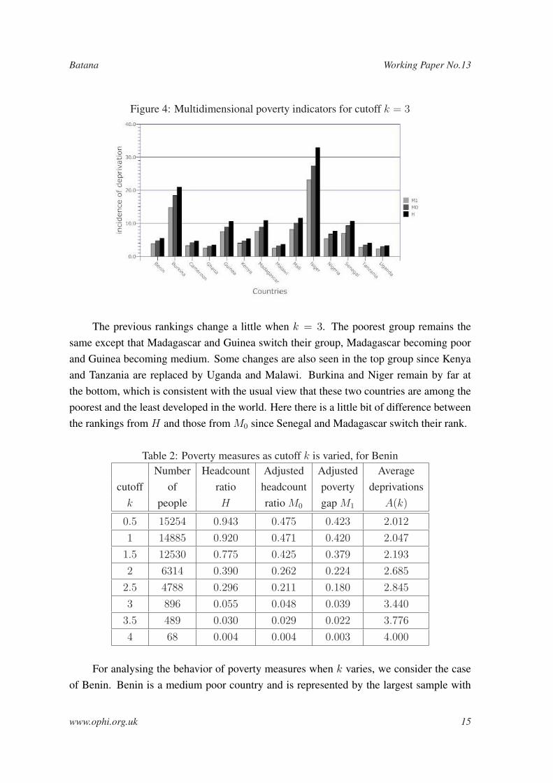
Figure 4: Multidimensional poverty indicators for cutoff k = 3

The previous rankings change a little when k = 3. The poorest group remains thesame except that Madagascar and Guinea switch their group, Madagascar becoming poorand Guinea becoming medium. Some changes are also seen in the top group since Kenyaand Tanzania are replaced by Uganda and Malawi. Burkina and Niger remain by far atthe bottom, which is consistent with the usual view that these two countries are among thepoorest and the least developed in the world. Here there is a little bit of difference betweenthe rankings from H and those from M0 since Senegal and Madagascar switch their rank.

Table 2: Poverty measures as cutoff k is varied, for BeninNumber Headcount Adjusted Adjusted Average

cutoff of ratio headcount poverty deprivationsk people H ratio M0 gap M1 A(k)

0.5 15254 0.943 0.475 0.423 2.012

1 14885 0.920 0.471 0.420 2.047

1.5 12530 0.775 0.425 0.379 2.193

2 6314 0.390 0.262 0.224 2.685

2.5 4788 0.296 0.211 0.180 2.845

3 896 0.055 0.048 0.039 3.440

3.5 489 0.030 0.029 0.022 3.776

4 68 0.004 0.004 0.003 4.000

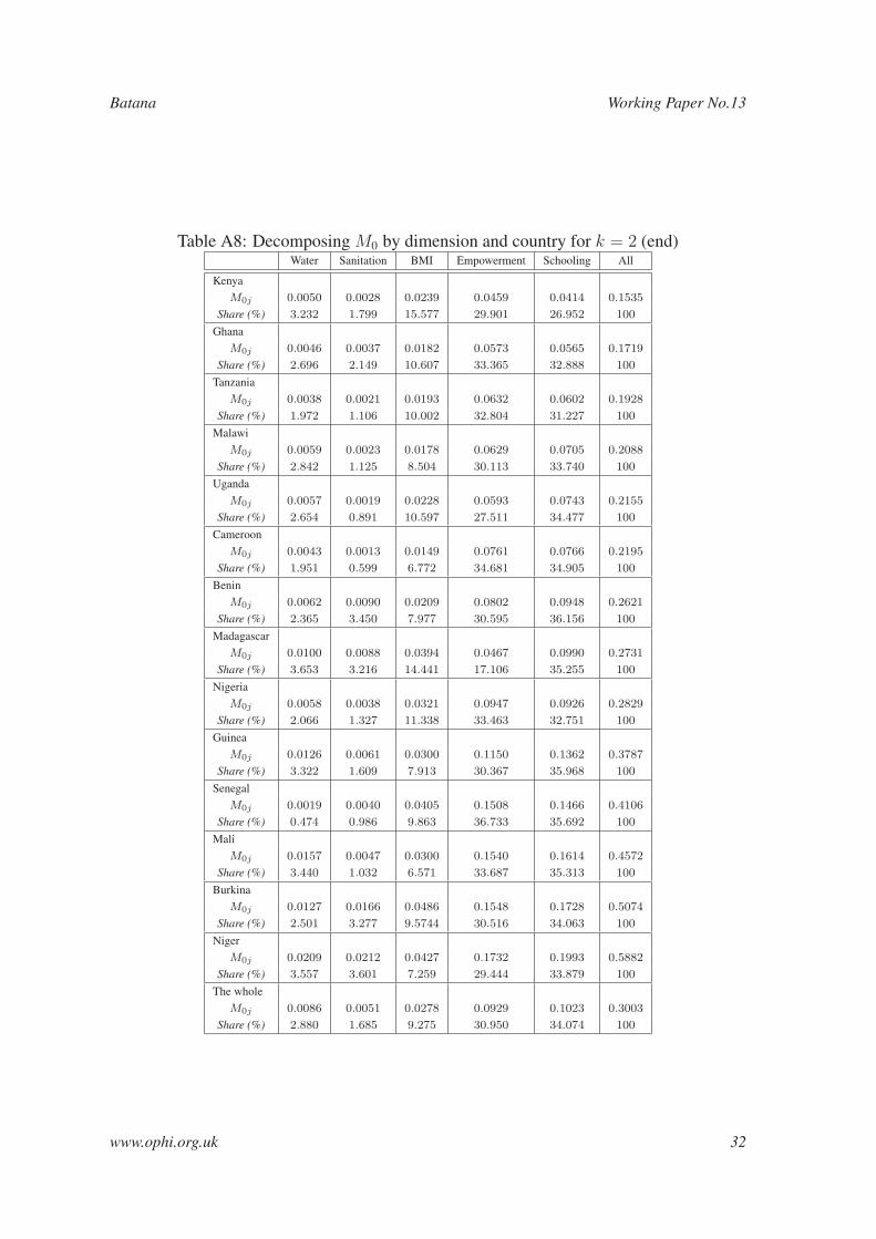
For analysing the behavior of poverty measures when k varies, we consider the caseof Benin. Benin is a medium poor country and is represented by the largest sample with

www.ophi.org.uk 15


16172 observations. The main results are presented in table 2. As expected, all measures(H ,M0,M1) decrease when k increases. Indeed, an increase in k is seen as a decrease inpoverty line. The variable A(k) in the last column is obtained by multiplying A in equation(5) by d the number of dimensions. It represents the average number of deprivations inthe poor people. For any k, as the poor individuals are identified as those with at least k

deprivations, then A(k) ≥ k. If there is at least any individual deprived in all dimensions,then A(k) > k when k < d and A(d) = d. When k = 0, A(k) becomes simply theaverage number of deprivations in the pooled populations. The estimated A(0) is 1.93. M0

and M1 differ from H by taking account of this relative depth of deprivation in povertymeasurement. For instance, M0 will be close to H only if poor people tend to be deprivedin all dimensions.

For k = 1, the poverty is overestimated since the multidimensional headcount ratioH , which is the same as the FGT incidence of poverty, varies from 66% in Kenya to 98%in Niger. For k = 3, that is the opposite case. The incidence of poverty varies from 3%in Uganda to 33% in Niger. Poverty appears underestimated since it is unthinkable that, ina developing country like Uganda, only 3% of women can be considered as poor. On theother hand, for k = 2, H take values between 22% in Kenya and 81% in Niger. This resultseems more reasonable and is in accordance with the previous results, including the WorldBank findings that, in average, about 50% of individuals are poor in Sub-Saharan Africa.Then, the cutoff k = 2 may be considered as suitable enough for doing some analysesincluding the comparisons with the standard poverty measures.

3.3 Comparisons with some standard measures

We now compare these findings with two standard poverty measures: income povertyand human development index (HDI). This is useful to capture the changes in the povertyassessment induced by the current multidimensional measure. The country rankings fromthe current multidimensional poverty measure are plotted against the rankings obtainedwhen using the two alternative measures. Figure 5 presents the comparison results fork = 2.

When rankings according two measures are identical, all the points in the graph, rep-resenting each country, should be on the 45-degree line. Since the measures used in thispaper go beyond the standard ones in the sense of considering additional and uncommondimensions, we are not expecting to find strong correlations between them. Moreover,since the woman is the unit of analysis, the current estimated measures could reflect in acertain extent gender differences. Figure 5 shows that differences in rankings from M0 and

www.ophi.org.uk 16


those based on income poverty are substantial. Except for Mali and Ghana and Uganda in alittle measure, most countries shifted noticeably. These differences could also be partiallydue to the incompatibility between dates. The date of income poverty estimation variesfrom 1992 to 2006 according countries when M0 is estimated from DHS data posterior to2000 for all selected countries. A quite similar result is obtained by Sahn and Stifel (2000)who find substantial differences between the asset index rankings and the rankings basedon GDP per capita.

The differences are less marked between HDI and M0. All the points are closer to the45-degree line. Indeed Mali, Uganda, Ghana, Guinea, Burkina and Niger are on the line orvery close to it.

Figure 5: Countries ranking comparisons for k = 2

(a) Against income poverty (b) Against human development index

Our results are also compared with two additional measures: asset poverty and genderrelated development index (GDI). Figure 6 shows the comparison results for k = 2. Assetpoverty is estimated from the current method by considering only the eight indicators ofAssets. Each indicator is weighted to 1 and the poverty measured by M0 for k = 4. Theresults, illustrated in the part (a) of the figure 6, suggest significant differences in rankings.This is due to the fact that the dimensions are uncorrelated or weakly correlated. For exam-ple, Senegal which is the best with asset poverty appears among the poorest countries whenwe take account of the three other dimensions. When the correlations between dimensionsare perfect, the findings will be unchanged whatever the number of dimensions which areconsidered. Then, the differences in rankings are more important when the correlationsdecrease. The part (b) of figure shows the comparison with GDI. The differences are less

www.ophi.org.uk 17


Figure 6: Countries ranking comparisons for k = 2

(a) Against asset poverty (b) Against gender related development index

important than in the part (a). The result is almost identical to the one obtained in part (b)of figure 5 because HDI and GDI induce very closed rankings. The detailed results areprovided in tables A4, A5 and A6 in appendices.

On the whole, the adding of schooling, health and empowerment allows us to bet-ter capture multidimensional poverty in the sense of Sen (1976; 1985; 1992; 1995). Thiscreates poverty measures more suitable and a little different from the standard and previ-ous indicators. Indeed, restricting the poverty analysis only to the assets, like in previousstudies on Africa, leads often to incorrectly capture poverty since there is many other well-being dimensions. Moreover, the consideration of a larger number of dimensions is likelyto reduce the effect of the discontinuities in each dimension on the aggregate poverty mea-sure.

4 Decomposing poverty

4.1 Decomposing by location

Decomposition is a useful property allowing to analyse poverty by subgroups. It isthen straightforward to implement better poverty-reducing policies by targeting the kinds ofdeprivations affecting each subgroup. The poverty measures, when k = 2, are decomposedby urban and rural location in all the countries and findings are illustrated in figure 7.

www.ophi.org.uk 18


This figure compares rural and urban poverty for the adjusted multidimensional head-count ratio. It suggests unambiguously a difference in poverty between urban and rurallocations. In all countries, rural people appear to be more poorer than urban people. This isnot surprising since such outcomes were ready observed in the previous studies. Using var-ious welfare indicators (asset poverty, enrollment, infant mortality rate, adult malnutrition,etc.), Sahn and Stifel (2003b) show that standards of living in rural areas are lower thanthose in urban areas in African countries. Booysen, Von Maltitz, Van der Berg, Burger, andDu Rand (2008) obtain a quite similar results with asset poverty. Using household expendi-tures per capita and children’s height-for-age z score as the two dimensions of well-being,Duclos, Sahn, and Younger (2006a) test stochastic dominance relations between rural andurban areas in Ghana, Madagascar and Uganda. They also find that rural areas are poorerthan the urban areas.

Figure 7: Decomposition of adjusted headcount M0 by urban and rural area, for k = 2

But the inequality in poverty between rural and urban areas seems to differ acrosscountries. From figure 7, one can notice that, for some relatively less poor countries likeKenya, Ghana, Malawi, Cameroon, Tanzania and Uganda, the incidence of poverty is atleast twice as high in rural areas as in urban ones. This is not the case for the poorest coun-tries (Mali, Niger, Senegal, Guinea). Burkina is the only poor country where the imbalanceis marked like in the former countries. Benin, which is a medium poverty country, displaysone of the most balanced poverty situations since the difference between rural poverty andurban poverty is relatively low. The appreciable urban-rural inequality observed in Burk-ina is underlined by Batana and Duclos (2008) from a dominance analysis. However, thisinequality, in our multidimensional measurement context, could be overestimated a littlesince some dimensions such as land and livestock owning, which is generally strongly

www.ophi.org.uk 19


valued in rural areas, are missing in the DHS database.

4.2 Decomposing by dimension

For assessing how the poverty is affected by the deprivations in each dimension, onecan decompose the adjusted ratio M0 into dimensions. The straightforward way for do-ing it is to disaggregate A in equation (5) into the four dimensions and eleven indicators.Let Aj be the contribution of dimension j in A. Aj could be interpreted as the averagedeprivation share across the poor in dimension j. The dimensional adjusted ratio M0j isthen obtained like in equation (6), by multiplying H and Aj . Dimensional decompositionis done when k = 2 for all countries, and the main results are reported in tables A7 andA8 in appendices. It is obvious that such a decomposition reflects a lot the differences inincidence of deprivation as shown in tables A2 and A3 and in figure 1.

Figure 8: Decomposition of adjusted ratio M0 by dimension as k is varied for the pool ofcountries

0.00 0.25 0.50 0.75 1.00 1.25 1.50 1.75 2.00 2.25 2.50 2.75 3.00 3.25 3.50 3.75 4.00

23

45

6

cutoff k

Share

in

ad

just

ed

rati

o M

0

Electricity Refrigerator Floor Water

Media Vehicle Phone Sanitation

(a) Nested components of assets

0.00 0.25 0.50 0.75 1.00 1.25 1.50 1.75 2.00 2.25 2.50 2.75 3.00 3.25 3.50 3.75 4.00

51

01

52

02

53

035

40

cutoff k

Sh

are

in a

dju

sted

rati

o M

0

Asset BMI Empowerment Schooling

(b) Four dimensions

Figure 8 describes the behavior of the dimensional adjusted ratio M0j for Benin whenk is varied. Concerning asset indicators, whose shares are plotted in the part (a), it is clearthat deprivations in refrigerator and telephone contribute the most to the poverty for any k.The other most influential indicators, according to their poverty contribution, are in orderelectricity, sanitation and vehicle owning. The floor quality and the drinking water accessare a third group of contributors less important than the previous. Finally, radio and/or TV(media) owning appears to contribute the least to poverty. The ranking between the abovefour groups of contributors is robust to the variation in k.

www.ophi.org.uk 20


The sum of the shares of nested dimensions gives the total share in M0 for assets.The part (b) of figure 8 shows that the rankings in contribution of poverty depend lightlyon k. For k ≤ 1.5, the contributions remain stable for the four dimensions. Schoolinghas the biggest contribution (44%), followed by assets (31%) and empowerment ((21%))respectively, while BMI has a negligible contribution (4%). From k = 1.5, the contributionsof schooling and assets begin to decline while those for empowerment and BMI start toincrease. From k = 1.875, empowerment become the second contributor behind schooling.Finally, the contribution of BMI which is almost marginal with low levels of k, starts toincrease significantly from k = 1.75. This coincides with a decline in other dimensions.Indeed, since the sum of contributions is 100, then a decrease in any dimension is balancedby an increase in another dimension.

Figure 9: Decomposition of multidimensional poverty by dimension for each country andfor k = 2

Figure 9 presents, for k = 2, the contributions of the four dimensions to the poverty.Burkina, Guinea and, in the little extent, Malawi display results close to Benin since school-ing appears to be the most contributor, followed respectively by by empowerment and as-

www.ophi.org.uk 21


sets. In countries like Cameroon, Ghana, Mali, Nigeria, Senegal and Tanzania, the con-tributions of schooling and empowerment are almost the same and both are higher thanthe assets contribution. The contributions of these three dimensions are quiet equal inKenya while only empowerment and assets have the same contribution, a little lower thanthe schooling contribution, in Niger and Uganda. Finally, the poverty in Madagascar isexplained mainly by schooling and assets. On the whole, BMI has a weak contributionwith a relative high level in Kenya and Madagascar. This decomposition of contribution bycountry could be helpful for suggesting better sectorial poverty-reducing policies.

5 Robustness analysis

5.1 Variations in cutoff k

To analyse whether the country rankings are robust across k, we implement themethodological approach in subsection 2.3. Figure 10 illustrates some dominance relationsfrom a sub-sample of countries including two highest poverty countries (Burkina, Niger),two medium countries (Benin, Nigeria) and two countries with relatively low poverty level(Ghana and Kenya). Each curve in the figure describes the poverty level in the countrywhen k is varied. Dominance is then possible between two countries when any curve liesabove or below another for all possible values of k. When two curves cross, there is nopossibility of dominance. In the two graphs of the figure, no dominance relation existsbetween Ghana and Kenya, Benin and Nigeria or Burkina and Niger since all these pairsof curve intersect. There are yet possibilities of dominance between any country from onepair and any country from another pair.

Several relations are identified from the full sample of countries and are tested underthe null hypothesis of non dominance against the alternative of dominance. The results arereported in tables 3 and 4, respectively for H and M0.

In the case of H , 42 dominance relations are proved to be significant at 5% level, outof the combination of C2

14 = 91 possible relations. Niger is dominated by all countriesexcept Burkina. Moreover, Ghana, Kenya and Cameroon dominate the five other poorestcountries that are Nigeria, Senegal, Guinea, Mali and Burkina. Some of these dominancerelations are restricted in the sense that they are found to be significant only for a reasonablerestricted range of k. There is no dominance between the eight first countries ranked as bythe table A5.

The non dominance relations, especially when curves intersect, could partly denote

www.ophi.org.uk 22


Figure 10: Poverty comparisons for some countries as k is varied

0.00 0.25 0.50 0.75 1.00 1.25 1.50 1.75 2.00 2.25 2.50 2.75 3.00 3.25 3.50 3.75 4.00

0.1

0.2

0.3

0.4

0.5

0.6

0.7

0.8

0.9

1.0

cutoff k

Head

cou

nt

rati

o H

Benin Burkina Ghana Kenya Niger Nigeria

(a) Comparisons in H

0.00 0.25 0.50 0.75 1.00 1.25 1.50 1.75 2.00 2.25 2.50 2.75 3.00 3.25 3.50 3.75 4.000

.10.2

0.3

0.4

0.5

0.6

cutoff kA

dju

sted

Head

cou

nt

rati

o M

0

Benin Burkina Ghana Kenya Niger Nigeria

(b) Comparisons in M0

Table 3: Results of dominance in headcount ratio H for all countriesGha Ken Cam Tan Mwi Uga Ben Mad Nga Sen Gui Mli Bur Ngr

Ghana − ND ND ND ND ND ND ND D D∗ D D D∗ D

Kenya − ND ND ND ND ND ND D∗ D∗ D∗ D∗ D∗ D

Cameroon − ND ND ND ND ND D∗ D∗ D∗ D D∗ D

Tanzania − ND ND ND ND ND ND D∗ D D∗ D

Malawi − ND ND ND ND ND D∗ D D∗ D

Uganda − ND ND ND ND D∗ D∗ D∗ D∗Benin − ND ND ND D∗ D∗ D∗ D

Madagascar − ND ND ND ND D∗ D

Nigeria − ND ND D D∗ D

Senegal − ND ND D∗ D

Guinea − ND ND D

Mali − ND D∗Burkina − ND

Niger −ND: non dominance; D: dominance; D∗: restricted dominance obtained for at least 0.5 ≤ k ≤ 3.5.

possible discontinuities in deprivations along k. These discontinuities are illustrated bythe sharp bends observed in the curves of figure 10. Since the headcount curves couldbe seen as cdfs for a decreasing series of k, this means that density curves are lumpy.The lumps are induce by the nested dimensions. In fact, the decimal values of k describefour superimposed distributions respectively for the intervals [0, 1], [1, 2], [2, 3] and [3, 4].Except for the discontinuities, the non dominance could be obviously explained by the mainmoments of the distribution that are mean and variance in the case of a normal distribution.The curves representing M0 appear to be smoother than those for H , particularly for k

lower than 2. This leads us to expect more dominance relations in the case of M0.

Indeed, with M0, 14 additional dominance relations are obtained, that is a total of 56

www.ophi.org.uk 23


Table 4: Results of dominance in adjusted headcount ratio M0 for all countriesGha Ken Tan Mwi Cam Uga Ben Mad Nga Sen Gui Mli Bur Ngr

Ghana − ND ND ND D∗ ND ND D D D∗ D D D D

Kenya − ND ND ND ND ND ND D∗ D∗ D∗ D∗ D D

Tanzania − ND ND ND ND ND D∗ D∗ D D D D

Malawi − ND ND ND D ND D∗ D D D D

Cameroon − ND ND ND D D∗ D D D D

Uganda − ND ND ND ND D∗ D D D

Benin − ND ND D∗ D∗ D∗ D D

Madagascar − ND ND D D D D

Nigeria − D∗ ND D D D

Senegal − ND ND D D

Guinea − D∗ D D

Mali − D D

Burkina − ND

Niger −ND: non dominance; D: dominance; D∗: restricted dominance obtained for at least 0.5 ≤ k ≤ 3.5.

relations out of the 91. Here, Burkina and Niger are dominated by all other countries. Thisresult confirms that both countries are the worst in term of poverty and well-being. Ourdominance results differ from those obtained by Sahn and Stifel (2000). For instance, intheir findings, Senegal is in the top with Ghana and dominates countries such as Kenya,Tanzania, Cameroon, Uganda and Benin. That is understanding since Senegal is relativelybetter in asset-based well-being. On the whole, as in subsection 3.2, five francophonecountries appear to be the poorest.

5.2 Changes in thresholds selections

For analysing the effect of a change in thresholds on poverty measures, we modifysome definitions from table 1. Most of indicators remain unchanged, but the poverty cutoffsfor five indicators changed, including four nested dimensions (Media, vehicle, drinkingwater, sanitation) and the dimension schooling. This choice is explained by the possibilityto make some sensible changes in the poverty line. The previous set of thresholds could beseen as the MDG definition. Two additional sets of thresholds are defined, the first like astronger definition than MDG one and the second like a weaker definition. For example,in strong definition, a woman is considered as being deprived in schooling if her educationlevel in single years is low than 10. More details on the new definitions can be found in thetable 5.

We analyse whether the country rankings are affected by adopting on of the two alter-native definitions. For k = 2, the results are illustrated in figure 11. From MDG definition,choose strong definition induces a re-ranking of country except for the three bottom coun-

www.ophi.org.uk 24


Table 5: Alternative definitions of thresholdsDimension Strong definition Weak definition

Media If does not have TV and −radio

Vehicle If does not have at least If does not have at leasta car a bycicle

Water If does not have at least If does not have at leasta piped water a dug well water

Sanitation If does not have at least −a flush toilet

Schooling If highest education level < 10 If highest education level < 3

tries which are Mali, Burkina and Niger. In general, this re-ranking seems stronger withinthe least poor countries. The comparisons between MDG and weak definition shows somere-rankings, less important than in the previous case. The situation remains unchanged formost countries, especially the poorest.

Changes in poverty thresholds definition are likely to re-rank the countries and, so,could change the previous dominance analysis. This finding does not matter since it de-pends on the multivariate distribution of poverty indicators in each country. The sameconclusion may be found in univariate distribution, when two distributions intersect forany unidimensional poverty line z.

Figure 11: Country rankings sensitivity to changes in thresholds definition, with k = 2

(a) Against strong definition (b) Against weak definition

For analysing the evolution of the rankings when k is varied, a mean absolute differ-ence (MAD) is calculated as follows:

www.ophi.org.uk 25


MADk =1

J

J∑j=1

|Rj(k)−Rj(k)|,

where j represents each country, J the total number of countries, Rj(k) the rank of countryj from MDG definition and Rj(k) the rank of country j from alternative definition.

Figure 12: Evolution of mean absolute difference as k is varied

0.00 0.25 0.50 0.75 1.00 1.25 1.50 1.75 2.00 2.25 2.50 2.75 3.00 3.25 3.50 3.75 4.00

0.5

1.0

1.5

2.0

2.5

3.0

cutoff k

Mean

ab

solu

te d

iffe

ren

ce

H, for all countries M0, for all countries H, for the 5 poorest countries M0, for the 5 poorest countries

(a) MDG vs strong definition

0.00 0.25 0.50 0.75 1.00 1.25 1.50 1.75 2.00 2.25 2.50 2.75 3.00 3.25 3.50 3.75 4.00

0.5

1.0

1.5

2.0

2.5

cutoff k

Mean

ab

solu

te d

iffe

ren

ce

H, for all countries M0, for all countries H, for the 5 poorest countries M0, for the 5 poorest countries

(b) MDG vs weak definition

The MAD is estimated for each k and is illustrated in figure 12. Each graph presentsfour curves for H and M0, for all countries and for only the five bottom countries accordingthe MDG definition. In the whole, the poverty measures appear to be sensitive to thethresholds definition since MAD is strictly positive for most k. However, the depth ofthe re-ranking varies according k. In the case of MDG versus strong definition, it appearsrelatively low and stable for k ≤ 1.75. The curves for M0 are smoother than the ones forH . This figure also confirms that the bottom countries depict less change in rankings thanthe others. For instance, in the case of MDG versus weak definition, for k ≤ 2.625, thereis no re-ranking for these countries, which is shown in figure 11 for k = 2. This meansthat there are high likelihoods so that some dominance relations obtained in subsection 5.1hold across changes in thresholds definition, when these relations imply the domination ofone of the bottom countries.

The sensitivity of this poverty measure suggests that, for identifying the poor, oneshould select a set of thresholds reasonable enough so that a deprivation in any dimensionreflects ethically and consensually an aspect of poverty. In this way, MDG could be useful,as in this paper, for appealing to a suitable poverty identification.

www.ophi.org.uk 26


6 Conclusion

Since poverty is recognized as being multidimensional, many methods of aggregationare proposed in the literature. An important issue that arises is to identify the poor. Thisidentification concerns both the deprivation in each dimension and the poverty definitionacross all dimensions. Alkire and Foster (2007) suggest an intuitive method using count-ing approach that deals with this issue in the two stages of identification. Moreover, thismeasure satisfies several useful properties which allow, for instance, targeting and povertycomparisons over time and across countries or regions.

Basing on such an approach, this paper estimated multidimensional poverty in four-teen sub-Saharan African countries. The findings suggest, for convenience, three groups ofcountries, the first including the poorest countries with headcount ratio exceeding 50%, thesecond composed by the medium poor countries with ratio between 30 and 50%, and thethird by countries with ratio less than 30%. The differences between countries seem impor-tant since, for instance, poverty in the bottom country is many times higher than poverty inthe top country. Comparisons with some standard measures such as HDI, income poverty,GDI and asset poverty show that consider additional dimensions leads to country rank-ings different, in a certain extent, from the standard-based rankings. Decompositions byrural/urban location and by dimension are done, showing both that the poverty is higherin rural areas than in urban areas, and that the contributions in poverty of deprivations inschooling, empowerment and asset depend on each country. Some robustness and sensi-tivity analyses are implemented to capture the effect of variations in cutoff k and changesin thresholds. In the first case, many dominance relations are obtained denoting that a dif-ference in poverty between two countries is robust along the full range of k. The secondanalysis reveals the sensitivity of poverty measures to changes in thresholds.

On the whole, the proposed method seems to be suitable for measuring poverty in de-veloping countries such as those from Sub-Saharan Africa. The sensitivity issue suggeststo select the thresholds in an ethically and consensually reasonable way. In this paper,that is done by selecting some poverty lines using as far as is possible the MDG crite-rions. Another issue which arises with this approach is relating to the weighting. Noneof the weighting methods is proved to be the best. The poverty measurement approachused here does not provide a suitable method to address this matter. However, it gives thelatitude to assign weights to each dimension in positive or normative way. In this paper,four dimensions are equally and normatively weighted by 1, and one of them (assets) alsoequally divided into eight nested dimensions. Future extensions could consist in exploringthe effects of change in the weighting on the poverty measures.

www.ophi.org.uk 27


Appendices

Table A1: Characteristics of samples from DHSCountry Survey years Obs number Rural area (%)

Benin 2006 16172 57.9Burkina 2003 11864 76.6Cameroon 2004 4738 51.4Ghana 2003 5235 58.9Guinea 2005 3757 71.3Kenya 2003 6980 68.3Madagascar 2003 7541 35.4Malawi 2004 10864 86.5Mali 2006 13622 64.9Niger 2006 4396 66.7Nigeria 2003 7121 59.9Senegal 2005 4220 56.6Tanzania 2004 9598 75.9Uganda 2006 1742 87.7

Table A2: Incidence of deprivation (in percentage) in all dimensionsBenin Burkina Cameroon Ghana Guinea Kenya Madagascar

Electricity 70.1 87.3 50.3 50.1 79.0 82.3 77.0Media 21.2 29.3 28.8 23.9 30.1 20.0 35.7Refrigerator 93.0 93.4 83.7 76.9 90.5 93.6 96.1Vehicle 55.1 69.1 82.7 90.6 83.9 92.3 96.8Floor 39.7 58.1 46.8 11.8 53.1 61.4 66.9Phone 96.4 94.8 97.6 90.0 91.7 83.6 93.6Water 41.6 51.2 34.5 47.4 67.5 59.4 59.7Sanitation 61.7 67.2 6.1 23.5 28.2 14.9 41.7Asset 59.9 68.8 53.8 51.8 65.5 63.5 70.9

BMI 8.7 19.7 6.7 9.1 12.2 11.8 18.3

Empowerment 40.7 69.2 55.5 48.4 52.5 50.0 26.0

Schooling 81.9 87.1 46.0 42.9 88.4 26.7 69.9

www.ophi.org.uk 28


Table A3: Incidence of deprivation (in percentage) in all dimensions (end)Malawi Mali Niger Nigeria Senegal Tanzania Uganda

Electricity 91.7 80.1 88.7 47.0 46.3 86.8 91.6Media 31.7 21.7 40.3 21.8 7.8 35.3 31.6Refrigerator 96.2 93.9 96.0 80.0 73.4 94.2 96.8Vehicle 96.5 61.5 89.7 74.3 80.2 96.0 95.8Floor 76.8 71.8 85.4 33.4 30.5 70.8 78.5Phone 93.4 94.6 98.9 94.5 75.1 87.8 99.4Water 54.8 71.0 76.6 53.0 7.8 38.7 53.3Sanitation 13.9 18.4 79.1 23.7 17.5 13.5 12.5Asset 69.4 64.1 81.9 53.5 42.3 65.4 69.9

BMI 8.5 12.3 17.2 14.1 17.0 9.5 11.0

Empowerment 42.5 69.0 73.6 64.3 70.7 52.9 35.5

Schooling 58.1 88.2 92.7 50.2 78.5 39.7 62.7

Table A4: Countries ranking according several indicators for k = 1Adjust. head. Income poverty* HDI GDI Asset poverty**

ratio M0 ratio (2007, UNDP) (2007, UNDP) for k = 4Country Value Rank Value Rank Value Rank Value Rank Value Rank

Kenya 0.335 1 0.520 10 0.521 4 0.521 4 0.589 6Ghana 0.351 2 0.280 1 0.553 1 0.549 1 0.424 2Cameroon 0.375 3 0.410 8 0.532 3 0.524 3 0.429 3Tanzania 0.378 4 0.360 5 0.467 8 0.464 7 0.619 9Malawi 0.414 5 0.650 13 0.437 11 0.432 10 0.675 12Uganda 0.415 6 0.380 6 0.505 5 0.501 5 0.677 13Nigeria 0.436 7 0.340 4 0.470 7 0.456 8 0.435 4Madagascar 0.441 8 0.710 14 0.533 2 0.530 2 0.653 10Benin 0.471 9 0.290 2 0.437 10 0.422 11 0.527 5Senegal 0.518 10 0.330 3 0.499 6 0.492 6 0.307 1Guinea 0.543 11 0.400 7 0.456 9 0.446 9 0.610 8Mali 0.582 12 0.640 12 0.380 12 0.371 12 0.595 7Burkina 0.609 13 0.460 9 0.370 14 0.364 13 0.610 11Niger 0.662 14 0.630 11 0.374 13 0.355 14 0.794 14* Provided by World Development Indicators (WDI) online.

** Calculated by considering the asset indicators only, each indicator weighted to 1.

www.ophi.org.uk 29




Kenya 0.153 1 0.520 10 0.521 4 0.521 4 0.589 6Ghana 0.172 2 0.280 1 0.553 1 0.549 1 0.424 2Tanzania 0.193 3 0.360 5 0.467 8 0.464 7 0.619 9Malawi 0.209 4 0.650 13 0.437 11 0.432 10 0.675 12Uganda 0.216 5 0.380 6 0.505 5 0.501 5 0.677 13Cameroon 0.219 6 0.410 8 0.532 3 0.524 3 0.429 3Benin 0.262 7 0.290 2 0.437 10 0.422 11 0.527 5Madagascar 0.273 8 0.710 14 0.533 2 0.530 2 0.653 10Nigeria 0.283 9 0.340 4 0.470 7 0.456 8 0.435 4Guinea 0.379 10 0.400 7 0.456 9 0.446 9 0.610 8Senegal 0.411 11 0.330 3 0.499 6 0.492 6 0.307 1Mali 0.457 12 0.640 12 0.380 12 0.371 12 0.595 7Burkina 0.507 13 0.460 9 0.370 14 0.364 13 0.610 11Niger 0.588 14 0.630 11 0.374 13 0.355 14 0.794 14* Provided by World Development Indicators (WDI) online.




Uganda 0.030 1 0.380 6 0.505 5 0.501 5 0.677 13Ghana 0.031 2 0.280 1 0.553 1 0.549 1 0.424 2Malawi 0.032 3 0.650 13 0.437 11 0.432 10 0.675 12Tanzania 0.035 4 0.360 5 0.467 8 0.464 7 0.619 9Cameroon 0.042 5 0.410 8 0.532 3 0.524 3 0.429 3Kenya 0.047 6 0.520 10 0.521 4 0.521 4 0.589 6Benin 0.048 7 0.290 2 0.437 10 0.422 11 0.527 5Nigeria 0.068 8 0.340 4 0.470 7 0.456 8 0.435 4Guinea 0.089 9 0.400 7 0.456 9 0.446 9 0.610 8Senegal 0.093 11 0.330 3 0.499 6 0.492 6 0.307 1Madagascar 0.089 10 0.710 14 0.533 2 0.530 2 0.653 10Mali 0.101 12 0.640 12 0.380 12 0.371 12 0.595 7Burkina 0.184 13 0.460 9 0.370 14 0.364 13 0.610 11Niger 0.274 14 0.630 11 0.374 13 0.355 14 0.794 14* Provided by World Development Indicators (WDI) online.


www.ophi.org.uk 30


Table A7: Decomposing M0 by dimension and country for k = 2Electricity Media Refrigerator Vehicle Floor Phone

KenyaM0j 0.0064 0.0027 0.0067 0.0066 0.005 0.0064

Share (%) 4.199 1.780 4.351 4.310 3.7108 4.189

GhanaM0j 0.0057 0.0023 0.0071 0.0074 0.0015 0.0076

Share (%) 3.293 1.332 4.104 4.284 0.866 4.417

TanzaniaM0j 0.0081 0.0037 0.0084 0.0084 0.0074 0.0081

Share (%) 4.211 1.913 4.353 4.363 3.837 4.211

MalawiM0j 0.0092 0.0039 0.0093 0.0093 0.0084 0.0092

Share (%) 4.416 1.868 4.476 4.457 4.040 4.420

UgandaM0j 0.0095 0.0044 0.0096 0.0096 0.0087 0.0097

Share (%) 4.403 2.037 4.458 4.444 4.049 4.480

CameroonM0j 0.0077 0.0040 0.0094 0.0083 0.0071 0.0099

Share (%) 3.497 1.812 4.272 3.774 3.231 4.507

BeninM0j 0.0098 0.0036 0.0117 0.0075 0.0065 0.0119

Share (%) 3.757 1.364 4.458 2.868 2.462 4.550

MadagascarM0j 0.0120 0.0079 0.0127 0.0127 0.0113 0.0126

Share (%) 4.394 2.898 4.640 4.635 4.134 4.629

NigeriaM0j 0.0082 0.0039 0.0120 0.0105 0.0065 0.0127

Share (%) 2.905 1.384 4.238 3.727 2.311 4.494

GuineaM0j 0.0146 0.0060 0.0163 0.0149 0.0108 0.0164

Share (%) 3.845 1.589 4.291 3.932 2.843 4.321

SenegalM0j 0.0105 0.0016 0.0156 0.0163 0.0071 0.0156

Share (%) 2.566 0.393 3.800 3.968 1.724 3.803

MaliM0j 0.0175 0.0050 0.0197 0.0132 0.0159 0.0198

Share (%) 3.826 1.100 4.319 2.898 3.477 4.337

BurkinaM0j 0.0206 0.0076 0.0214 0.0164 0.0144 0.0215

Share (%) 4.062 1.494 4.213 3.236 2.835 4.230

NigerM0j 0.0233 0.0120 0.0248 0.0232 0.0225 0.0251

Share (%) 3.964 2.037 4.209 3.947 3.830 4.274

The wholeM0j 0.0114 0.0047 0.0129 0.0115 0.0099 0.0130

Share (%) 3.812 1.576 4.300 3.825 3.301 4.324

www.ophi.org.uk 31


Table A8: Decomposing M0 by dimension and country for k = 2 (end)Water Sanitation BMI Empowerment Schooling All

KenyaM0j 0.0050 0.0028 0.0239 0.0459 0.0414 0.1535

Share (%) 3.232 1.799 15.577 29.901 26.952 100

GhanaM0j 0.0046 0.0037 0.0182 0.0573 0.0565 0.1719

Share (%) 2.696 2.149 10.607 33.365 32.888 100

TanzaniaM0j 0.0038 0.0021 0.0193 0.0632 0.0602 0.1928

Share (%) 1.972 1.106 10.002 32.804 31.227 100

MalawiM0j 0.0059 0.0023 0.0178 0.0629 0.0705 0.2088

Share (%) 2.842 1.125 8.504 30.113 33.740 100

UgandaM0j 0.0057 0.0019 0.0228 0.0593 0.0743 0.2155

Share (%) 2.654 0.891 10.597 27.511 34.477 100

CameroonM0j 0.0043 0.0013 0.0149 0.0761 0.0766 0.2195

Share (%) 1.951 0.599 6.772 34.681 34.905 100

BeninM0j 0.0062 0.0090 0.0209 0.0802 0.0948 0.2621

Share (%) 2.365 3.450 7.977 30.595 36.156 100

MadagascarM0j 0.0100 0.0088 0.0394 0.0467 0.0990 0.2731

Share (%) 3.653 3.216 14.441 17.106 35.255 100

NigeriaM0j 0.0058 0.0038 0.0321 0.0947 0.0926 0.2829

Share (%) 2.066 1.327 11.338 33.463 32.751 100

GuineaM0j 0.0126 0.0061 0.0300 0.1150 0.1362 0.3787

Share (%) 3.322 1.609 7.913 30.367 35.968 100

SenegalM0j 0.0019 0.0040 0.0405 0.1508 0.1466 0.4106

Share (%) 0.474 0.986 9.863 36.733 35.692 100

MaliM0j 0.0157 0.0047 0.0300 0.1540 0.1614 0.4572

Share (%) 3.440 1.032 6.571 33.687 35.313 100

BurkinaM0j 0.0127 0.0166 0.0486 0.1548 0.1728 0.5074

Share (%) 2.501 3.277 9.5744 30.516 34.063 100

NigerM0j 0.0209 0.0212 0.0427 0.1732 0.1993 0.5882

Share (%) 3.557 3.601 7.259 29.444 33.879 100

The wholeM0j 0.0086 0.0051 0.0278 0.0929 0.1023 0.3003

Share (%) 2.880 1.685 9.275 30.950 34.074 100

www.ophi.org.uk 32


References

ALKIRE, S. AND J. FOSTER (2007): “Counting and Multidimensional Poverty Mea-surement,” OPHI Working Paper Series No. 07, OPHI.

ANDERSON, G., I. CRAWFORD, AND A. LIECESTER (2005): “Statistical Tests forMultidimensional Poverty Analysis,” Brazilia, Brazil: International Conferenceon the Many Dimensions of Poverty.

ATKINSON, A. B. (1987): “On the Measurement of Poverty,” Econometrica, 55,749–764.

——— (2003): “Multidimensional Deprivation: Contrasting Social Welfare andCounting Approaches,” Journal of Economic Inequality, 1, 51–65.

BATANA, Y. M. AND J.-Y. DUCLOS (2008): “Multidimensional Poverty Dominance:Statistical Inference and an Application to West Africa,” CIRPÉE Working Paper08-08, CIRPÉE.

BOOYSEN, F., M. VON MALTITZ, S. VAN DER BERG, R. BURGER,AND G. DU RAND (2008): “Using an Asset Index to Assess Trendsin Poverty in Seven Sub-Saharan African Countries,” World Development,doi:10.1016/j.worlddev.2007.10.008.

BOURGUIGNON, F. AND S. R. CHAKRAVARTY (2003): “The Measurement of Mul-timensional Poverty,” Journal of Economic Inequality, 1, 25–49.

CERIOLI, A. AND S. ZANI (1990): “A Fuzzy Approach to the Measurement ofPoverty,” in Income and Wealth Inequality and Poverty, ed. by C. Dagum andM. Zenga, Berlin: Spring Verlag, 272–284.

CHELI, B. AND A. LEMMI (1994): “A Totally Fuzzi and Relative Approach to theMultidimensional Analysis of Poverty,” Economic notes, 24, 115–134.

CHIAPPERO-MARTINETTI, E. (2006): “Capability Approach and Fuzzy Set Theory:Description, Aggregation and Inference Issues,” in Fuzzy Set Approach to Mul-tidimensional Poverty Measurement, ed. by A. Lemmi and G. Betti, New york:Spring Verlag, 93–114.

DAVIDSON, R. AND J.-Y. DUCLOS (2006): “Testing for Restricted Stochastic Dom-inance,” IZA Discussion Paper No 2047, IZA.

DEUTSCH, J. AND J. SILBER (2005): “Measuring Multidimensional Poverty: AnEmpirical Comparison of Various Approaches,” Review of Income and Wealth,51, 145–174.

DI TOMMASO, M. L. (2007): “Children Capabilities: A Structural Equation Modelfor India,” The Journal of Socio-Economic, 36, 436–450.

DUCLOS, J.-Y., D. E. SAHN, AND S. D. YOUNGER (2006a): “Robust Multidimen-

www.ophi.org.uk 33


sional Spatial Poverty Comparisons in Ghana, Madagascar and Uganda,” WorldBank Economic Review, 20, 91–113.

——— (2006b): “Robust Multimensional Poverty Comparison,” Economic Journal,113, 943–968.

FOSTER, J. E., J. GREER, AND E. THORBECKE (1984): “A Class of DecomposablePoverty Measures,” Econometrica, 52, 761–766.

FOSTER, J. E. AND A. F. SHORROCKS (1988a): “Poverty Orderings and WelfareDominance,” Social Choice Welfare, 5, 179–198.

——— (1988b): “Poverty Orderings,” Econometrica, 56, 173–177.IBRAHIM, S. AND S. ALKIRE (2007): “Agency and Empowerment: A Proposal for

Internationally Comparable Indicators,” Oxford Development Studies, 35, 379–403.

KLASEN, S. (2000): “Measuring Poverty and Deprivation in South Africa,” Reviewof Income and Wealth, 46, 33–58.

KRISHNAKUMAR, J. (2007): “Going Beyond Functionings to Capabilities: AnEconometric Model to explain and Estimate Capabilities,” Journal of Human De-velopment, 8, 39–63.

KRISHNAKUMAR, J. AND P. BALLON (2008): “Estimating Basic Capabili-ties: A Structural Equation Model Applied to Bolivia,” World Development,doi:10.1016/j.worlddev.2007.10.006.

LOVELL, C. A. K., S. RICHARDSON, P. TRAVERS, AND L. WOOD (1994): “Re-sources and Functionings: A New View of Inequality in Australia,” in Modelesand Measurement of Welfare and Inequality, ed. by W. Eichhorn, Springer VerlagHeidelberg.

MAASOUMI, E. (1993): “A Compendium to Information Theory in Economics andEconometrics,” Econometric Reviews, 12, 1–49.

MAASOUMI, E. AND M. A. LUGO (2008): “The Information Basis of MultivariatePoverty Assessments,” in Quantitative Approaches to Multidimensional PovertyMeasurement, ed. by N. Kakwani and J. Silber, New York: Palgrave-MacMillan,1–29.

SAHN, D. E. AND D. C. STIFEL (2000): “Poverty Comparisons Over Time andAcross Countries in Africa,” World Development, 28, 2123–2155.

——— (2003a): “Exploring Alternative Measures of Welfare in the Absence of Ex-penditure Data,” Review of Income and Wealth, 49, 463–489.

——— (2003b): “Urban-Rural Inequality in Living Standards in Africa,” Journal ofAfrican Economies, 12, 564–597.

SEN, A. (1976): “Poverty: An Ordinal Approach to Measurement,” Econometrica,

www.ophi.org.uk 34


44, 219–231.——— (1985): Commodities and Capabilities, Amsterdam: North-Holland.——— (1992): Inequality Reexamined, Cambridge: Harvard University Press.——— (1995): “The Political Economy of Targeting,” in Public Spending and the

Poor: Theory and Evidence, ed. by D. van der Walle and K. Nead, Baltimore:Johns Hopkins University Press.

THOMAS, V., Y. WANG, AND X. FAN (2001): “Measuring Education Inequality:Gini Coefficients of Education,” Policy Research Working Paper No 2525, WorldBank: Washington DC.

TSUI, K.-Y. (2002): “Multidimensional Poverty indice?” Social Choice and Welfare,19, 69–93.

UNITED NATIONS, . (2003): Indicators for Monitoring the Millennium DevelopmentGoals: Definitions, Rationale, Concepts and Sources, New York: United Nations.

VON MALTZAHN, R. AND K. DURRHEIM (2008): “Is Poverty Multidimensional? AComparison of Income and Asset based Measures in five Southern Africa Coun-tries,” Social Indicators Research, 86, 149–162.

WAGLE, U. (2005): “Multidimensional Poverty Measurement with Economic Well-being, Capability, and Social Inclusion: A case from Kathmandou, Nepal,” Jour-nal of Human Development, 6, 301–328.

WATTS, H. (1968): “An Economic Definition of Poverty,” in On UnderstandingPoverty, ed. by D. P. Moynihan, New York: Basic Books.

www.ophi.org.uk 35

Multidimensional Measurement of Poverty in Sub … · Multidimensional Measurement of Poverty in...

Documents

Transcript of Multidimensional Measurement of Poverty in Sub … · Multidimensional Measurement of Poverty in...