
Multidimensional grid technique - Vilniaus universitetasalgis/dsax/DDS-7-Grid.pdf · the record...
40
1 Multidimensional grid technique
Transcript of Multidimensional grid technique - Vilniaus universitetasalgis/dsax/DDS-7-Grid.pdf · the record...

1
Multidimensional grid technique

2
Grid file
• Increase database and integrated information systems usage
• File structures => efficient access to records:
• combine attribute values (multikeys)
• traditional file structures that provide multikey access to records are extensions of single-key access.
• they manifest various deficiencies in particular for multikey access to highly dynamic files

3
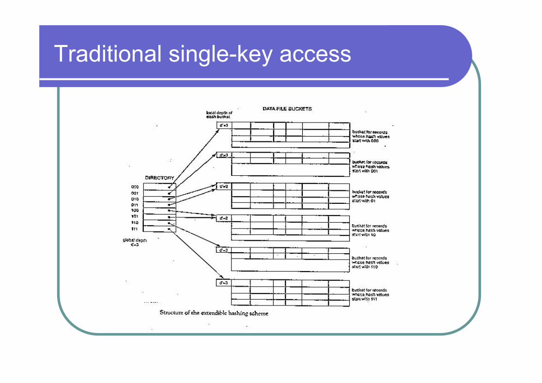
Traditional single-key access
• One dimensional case – hashing:
Hashing
Hashing Procedures Let us denote the set of all possible key values (i.e., the universe of keys) used in a dictionary application by U. Suppose an application requires a dictionary in which elements are assigned keys from the set of small natural numbers. That is, U � Z+ and ~U~ is relatively small. If no two elements have the same key, then this dictionary can be implemented by storing its elements in the array T[0, … , ~U~ - 1]. This implementation is referred to as a direct-access table since each of the requisite DICTIONARY ADT operations - Search, Insert, and Delete - can always be performed in 4(1) time by using a given key value to index directly into T, as shown:
The obvious shortcoming associated with direct-access tables is that the set U rarely has such "nice" properties. In practice, ~U~ can be quite large. This will lead to wasted memory if the number of elements actually stored in the table is small relative to ~U~. Furthermore, it may be difficult to ensure that all keys are unique. Finally, a specific application may require that the key values be real numbers, or some symbols which cannot be used directly to index into the table. An effective alternative to direct-access tables are hash tables. A hash table is a sequentially mapped data structure that is similar to a direct-access table in that both attempt to make use of the random-access capability afforded by sequential mapping. However, instead of using a key value to directly index into the hash table, the index is computed from the key value using a hash function, which we will denote using h. This situation is depicted as follows:
Traditional single-key access

5
Grid file
l The grid file l based on dynamic hashing for multi-attribute data
l two basic structures: k-linear scales + k-dimensional directory
l grid directory: k-dimensional array
l data page is allowed to store objects from several grid cells as long as the union of these cells from a rectangle, storage region

Grid file
l Grid partition of the search space: l problem: spatial queries in k-d point-sets l main idea: try to generalize hashing to k-d
4
size of this bitmap is impossibly large. Since this bitmap contains a lot of zeros, it can be
compressed. Here we need a compression scheme, that is compatible with the operations
executed on a file. FIND, INSERT and DELETE must be executed efficiently.
2.2 Grid Partition of the Search Space
2.2.1 Grid Blocks
The partitions are obtained by dividing the domain of each attribute into intervals.
Example for the two-dimensional case (generalization to k dimensions is obvious):
Figure 1: Grid Partition of the Search Space
As seen in Figure 1, on the record space S = X x Y we obtain a grid partition P = U x W
by imposing intervals U = (u0, u1, u2, u3), V = (v0, v1, v2, v3) on each axis and dividing
the record space into blocks, which we call grid blocks. With grid partitions each
boundary cuts the entire search space into two. All dimensions are treated symmetrically.
A file structure allocates storage in units of fixed size, called disk blocks, pages or
buckets, depending on the level of description. A storage unit, that contains records, is
called bucket. A bucket has a capacity c, which is the number of records it can contain.
2.2.2 Partition Modification
The grid partition is dynamic and can be modified. The grid partition P = U x V is
modified by altering only one of its components at a time. A one-dimensional partition is
modified by splitting one of its intervals, or by merging two adjacent intervals into one.
u2 u1 u0
v2
v1
v0
X
Y
u3
v3

7
Initial approach of locational data 16-4 Handbook of Data Structures and Applications
(27,35)Omaha
(52,10)Mobile
(62,77)Toronto
(82,65)Buffalo
(85,15)Atlanta
(90,5)Miami
(35,42)Chicago
(0,100) (100,100)
(100,0)(0,0)
y
x
(45,30)Memphis
FIGURE 16.1: Uniform-grid representation corresponding to a set of points with a searchradius of 20.
scales are usually implemented as one-dimensional trees containing ranges of values.The array access structure is fine as long as the data is static. When the data is dynamic,
it is likely that some of the grid cells become too full while other grid cells are empty. Thismeans that we need to rebuild the grid (i.e., further partition the grid or reposition thegrid partition lines or hyperplanes) so that the various grid cells are not too full. However,this creates many more empty grid cells as a result of repartitioning the grid (i.e., emptygrid cells are split into more empty grid cells). The number of empty grid cells can bereduced by merging spatially-adjacent empty grid cells into larger empty grid cells, whilesplitting grid cells that are too full, thereby making the grid adaptive. The result is that wecan no longer make use of an array access structure to retrieve the grid cell that containsquery point p. Instead, we make use of a tree access structure in the form of a k-ary treewhere k is usually 2d. Thus what we have done is marry a k-ary tree with the fixed-gridmethod. This is the basis of the point quadtree [22] and the PR quadtree [56, 63] whichare multidimensional generalizations of binary trees.
The difference between the point quadtree and the PR quadtree is the same as thedifference between trees and tries [25], respectively. The binary search tree [45] is an exampleof the former since the boundaries of different regions in the search space are determinedby the data being stored. Address computation methods such as radix searching [45] (alsoknown as digital searching) are examples of the latter, since region boundaries are chosenfrom among locations that are fixed regardless of the content of the data set. The process isusually a recursive halving process in one dimension, recursive quartering in two dimensions,etc., and is known as regular decomposition.
In two dimensions, a point quadtree is just a two-dimensional binary search tree. The firstpoint that is inserted serves as the root, while the second point is inserted into the relevantquadrant of the tree rooted at the first point. Clearly, the shape of the tree depends onthe order in which the points were inserted. For example, Figure 16.2 is the point quadtree
Buffalo, Memphis, Omaha, Atlanta, and Miami.
© 2005 by Chapman & Hall/CRC
corresponding to the data of Figure 16.1 inserted in the order Chicago, Mobile, Toronto,

Grid file
l Special kind of hashing l Adaptable: w.r.t. insert/delete
l Efficient query handling l Dynamic : Access time is uniform (two-disk-access
principle) l Symmetric: No Secondary Key. Every key is the
Primary Key l Multikey: records using subset of keys

Grid file Point Access Methods
Multidimensional Hashing
Grid File
BANG File

Grid file

l useful for range queries that would map into a set of cells corresponding to a group of values along the linear scales.
l can be applied to any number of search keys:
l n search keys => n dimensions.
l they perform well in terms of reduction in time for multiple key access.
Grid file

Grid file – how?
l Divide record space into grid blocks

l Allocates storage in units of fixed size l Disk blocks/pages/buckets
l To map grid blocks to buckets ?
l Use grid directory
l Two-disk-access: Retrieve single record in at-most 2 disk access
l Access directory(grid)
l Access Bucket(database)
l Efficient range queries
Grid file

Grid Directory (k=2)

Single Record Access [1980,w]
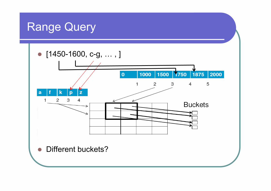
Range Query
l [1450-1600, c-g, … , ]
l Different buckets?

Next in each direction
l Nextxabove: cx = (cx+1) mod nx l Nextxbelow: cx = (cx-1) mod nx
l Nextyabove: cy = (cy+1) mod ny
l Nextybelow: cy = (cy-1) mod ny

Insertion
l Bucket size = 4
l Split it

Grid File Insertion

Grid File Insertion

Grid File Insertion
l Fixed scheduled Dimension splitting is used in this example

Directory Merging
l No queries between [a-k] and [0-1500]
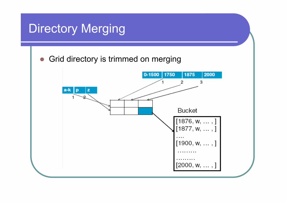
Directory Merging
l Grid directory is trimmed on merging

Concurrent access
l No root node as in trees, allows concurrency
Advantages
l No special computations are required l Only the right records are retrieved
l Can also be used for single search key queries
l Easy to extend to queries on n search keys
l Significant improvement in processing time for multiple-key queries
l Has a two-disk-access upper bound for accessing data
l Allows simpler concurrency control protocols

Grid files - disadvantages
l #1: problems in high-d: directory splits can be expensive
l #2: even in low-d, suffers on correlated attributes

Grid files - disadvantages
l (A1: rotate; A2: triangular cells)

Grid files - disadvantages
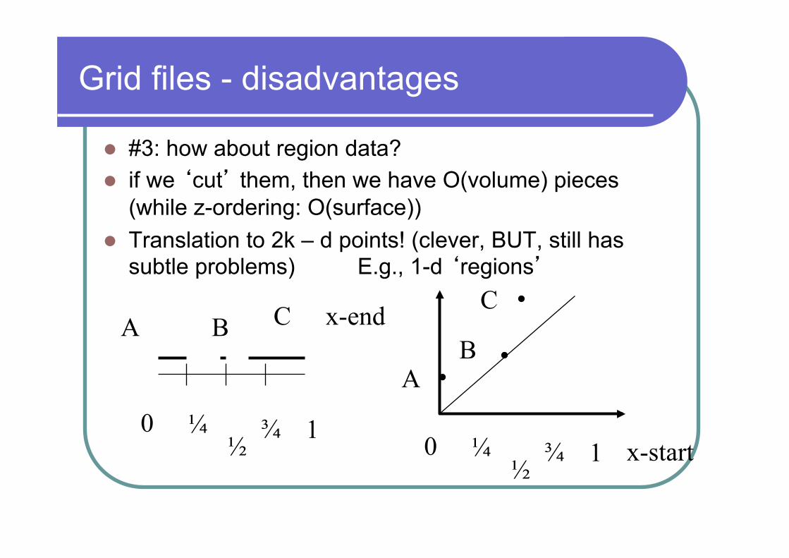
l #3: how about region data?
Grid files - disadvantages
l #3: how about region data? l if we ‘cut’ them, then we have O(volume) pieces
(while z-ordering: O(surface)) l Translation to 2k – d points! (clever, BUT, still has
subtle problems) E.g., 1-d ‘regions’
A B C
x-start
x-end
0 1 ½ ¼ ¾
0 1 ½ ¼ ¾
A B
C

Grid files - disadvantages
l what to do? l Translation to 2kd points! (clever, BUT, still has
subtle problems) E.g., 1-d ‘regions’
A B C
x-start
x-end
0 1 ½ ¼ ¾
0 1 ½ ¼ ¾
A B
C

Disadvantages
l dimensionality curse; large query regions l imposes space overhead
l performance overhead on insertion and deletion
l a frequent reorganization of the file adds to the maintenance cost

Bang file
l A BANG file (balanced and nested grid file) is a point access method which divides space into a nonperiodic grid.
l Each spatial dimension is divided by a linear hash.
l Cells may intersect, and points may be distributed between them.

Bang file
l It organizes the value space surrounding the data values, instead of comparing the data values themselves.
l Its tree structured directory partitions the data space into block regions with successive binary divisions on dimensions.
l The clustering algorithm identifies densely populated regions as cluster centers and expands those with neighboring blocks.

Bang file
Point Access Methods
Multidimensional Hashing
Grid File
BANG File
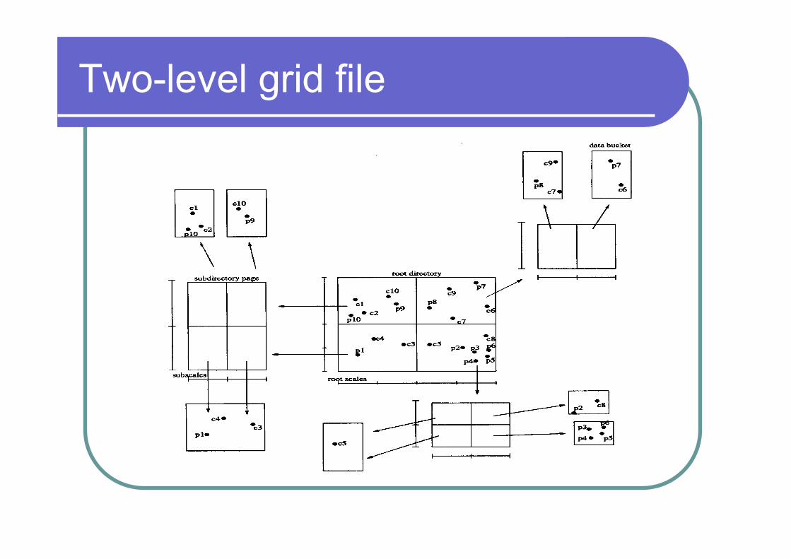
Two-level grid file Two-Level Grid File
Twin Grid File
Twin grid file
Two-Level Grid File
Twin Grid File
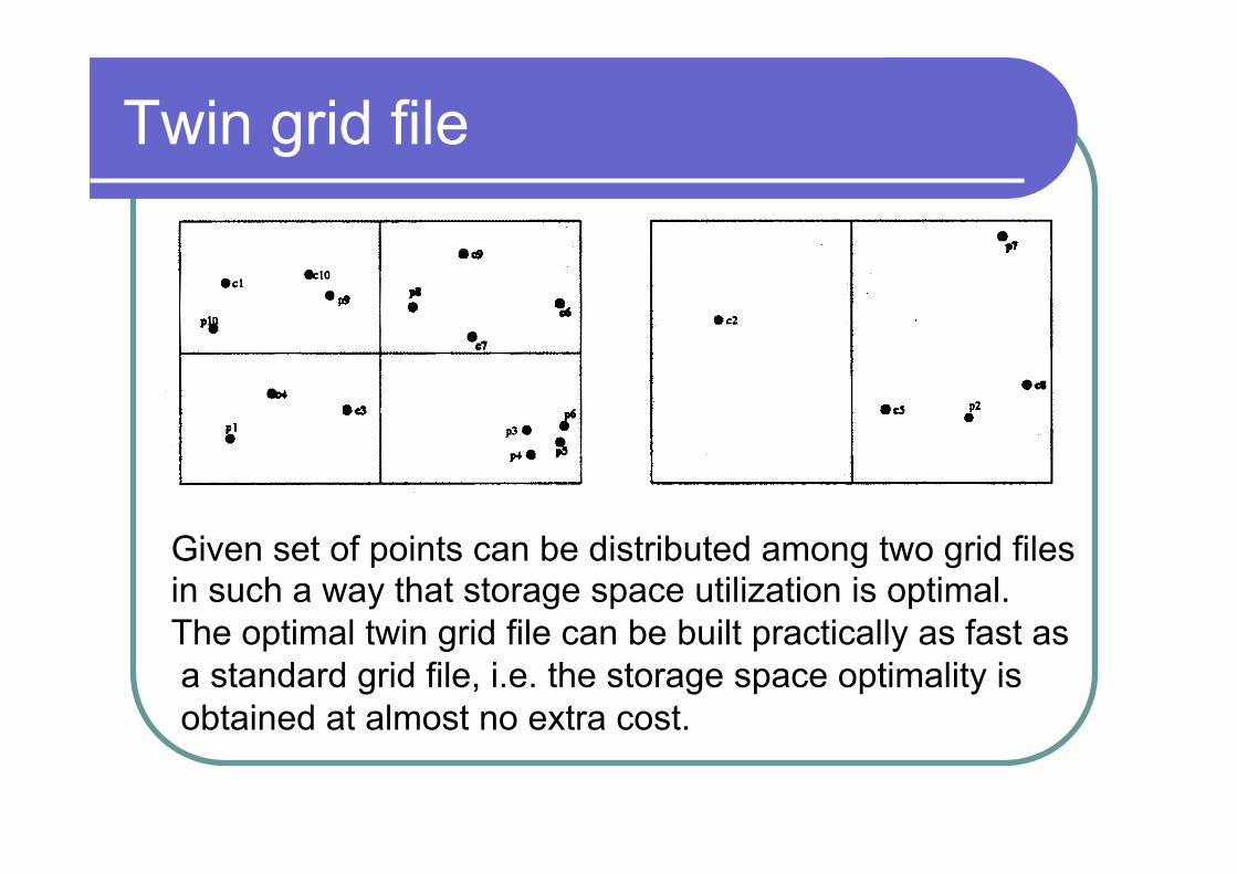
Given set of points can be distributed among two grid files in such a way that storage space utilization is optimal. The optimal twin grid file can be built practically as fast as a standard grid file, i.e. the storage space optimality is obtained at almost no extra cost.

Twin grid file
The performances of the standard grid file, the optimal static twin grid file, and an efficient dynamic twin grid file, where insertions and deletions trigger the redistribution of points among the two grid files.
Twin grid files utilize storage space at roughly 90%, as compared with the 69% of the standard grid file.
Typical range queries - the most important spatial search operations - can be answered in twin grid files at least as fast as in the standard grid file.

Buddy tree The buddy tree is a dynamic hashing scheme with a tree-like directory. The universe is cut recursively into two parts of equal size with iso-oriented hyperplanes, and each interior node corresponds to a partition together with interval. The interval corresponds to MBB, covering points below of given node. Also: l Each directory node contains at least two entries; l Whenever a node is split, the MBB and subnodes are
recomputed, to fit situation; l Except for the root of the directory, there is exactly one
pointer referring to each directory page.
Buddy tree Buddy Tree
The buddy tree is a dynamic hashing scheme with a tree-like directory. The
universe is cutted recursively into two parts of equal size with iso-oriented
hyperplanes, and each interior node corresponds to a partition together with
interval. The interval corresponds to MBB, covering points below of given
node. Also:
• Each directory node contains at least two entries;
• Whenever a node is split, the MBB and subnodes are recomputed, to fit
situation;
• Except for the root of the directory, there is exactly one pointer referring to
each directory page.

Buddy tree
of the @J&IV Tra - The buddy-tree organizes data using a tree-based directory where each axis is treated equally. In contrast to the K-D- B-tree Rob811 (one of the first multidimensional trees), the buddy-tree performs well in a highly dynamic environment, i. e. insertions, deletions and a change of the data distribution do not affect performance. This property is achieved by applying a modified version of the so-called buddy-system which is well-known from the grid file [NHS84] to the buddy-tree. Additionally, the performance of the buddy-tree is almost independent of the sequence of insertions which is an essential drawback of previous tree-structures, like the K-D-B-tree or hB-tree lLS891.
Another important feature of the buddy-tree is that it does not partition empty data space. Therefore queries, such as partial match queries, where the query region intersects with empty data space, can be performed much faster than by conventional structures partitioning the complete data space. This property is very similar to the variants of the R-tree, originally designed for spatial data Con&u-y to the R-tree, the buddy-tree does not allow overlap in the directory nodes and can therefore guarantee that insertions, deletions and exact match queries are restricted to one path of the directory. Additionally, we incorporate an implementation technique in the buddy-tree which in-creases the fan out of the directory nodes (see section 4).
The following catalogue summarizes the design properties of the buddy-tree:
l empty data space is not partitioned l insertion and deletion of a record is restricted to
exactly one path l no overflow pages l directory grows linear in the number of records l performance is basicly independent of the sequence of
insertions l efficient behavior for insertions and deletions l very high fan out of the directory nodes
With the following example we intend to visualize the basic properties of the buddy-tree:
Let the dimension be d = 2, the capacity of a directory page be c = 5 and the capacity of a data page be b = 4. Then the following snapshots depict the growth of the buddy-tree starting with the empty file. In the data pages the actual points are stored. Minimum bounding rectangles of at most 4 points are represented in the directory pages indicated by a light fill pattern. The white area corresponds to empty data space which is not managed by the buddy-tree (important design property). The first line in our example shows states of the buddy- tree with an overflowing data page depicted by a dark fill pattern. In the second line the corresponding subsequent state after the page split is depicted. The rightmost overflow of a data page implies an overflow of the one and only directory page resulting in a buddy-tree of height two.
592
.