Graduate Theses, Dissertations, and Problem Reports

2019

Multidimensional Analysis of Vulnerability: Methodological Multidimensional Analysis of Vulnerability: Methodological

Advances and a Case Study from Malawi. Advances and a Case Study from Malawi.

PARK MCMILLAN MUHONDA pmmuhonda@mix.wvu.edu

Follow this and additional works at: https://researchrepository.wvu.edu/etd

Part of the Human Geography Commons, Physical and Environmental Geography Commons, and the

Spatial Science Commons

Recommended Citation Recommended Citation MUHONDA, PARK MCMILLAN, "Multidimensional Analysis of Vulnerability: Methodological Advances and a Case Study from Malawi." (2019). Graduate Theses, Dissertations, and Problem Reports. 7459. https://researchrepository.wvu.edu/etd/7459

This Dissertation is protected by copyright and/or related rights. It has been brought to you by the The Research Repository @ WVU with permission from the rights-holder(s). You are free to use this Dissertation in any way that is permitted by the copyright and related rights legislation that applies to your use. For other uses you must obtain permission from the rights-holder(s) directly, unless additional rights are indicated by a Creative Commons license in the record and/ or on the work itself. This Dissertation has been accepted for inclusion in WVU Graduate Theses, Dissertations, and Problem Reports collection by an authorized administrator of The Research Repository @ WVU. For more information, please contact researchrepository@mail.wvu.edu.

Multidimensional Analysis of Vulnerability: Methodological Advances and a Case Study

from Malawi.

Park M.N.M. Muhonda

Dissertation submitted

to the Eberly College of Arts and Sciences

at West Virginia University

in partial fulfillment of the requirements for the degree of

Doctor of Philosophy in

Geography

Brent McCusker, Ph.D., Chair

Jamison Conley, Ph.D.

Eungul Lee, Ph.D.

Bradley Wilson, Ph.D.

Edward Carr, Ph.D.

Department of Geology and Geography

Morgantown, West Virginia

2019

Keywords: Malawi, livelihood vulnerability, spatial vulnerability analysis, adaptation to

climate change, local perceptions, climate variability

Copyright 2019 [Park M.N.M. Muhonda]

Abstract

Multidimensional Analysis of Vulnerability: Methodological Advances and a Case Study

from Malawi.

Park M.N.M. Muhonda

Since 1990s rural households in Malawi, constituting 85% of the population, have experienced

deepening livelihood vulnerability, often manifested as persistent food insecurity. Livelihood

crises have since been blamed on or attributed directly to weather perturbations/climatic shocks

i.e. El-Nino induced climate variability/drought conditions. This study revealed that persistent

livelihood crisis in rural Malawi cannot be attributed to or squarely blamed on weather shocks

alone, rather it is at the intersection of various livelihoods shocks that rural livelihood vulnerability

in Malawi is exacerbated i.e. worsening and deepening.

Thus, rural livelihood vulnerability to climate shocks in Malawi is manifest not in isolation but in

relation to a wide range of other shocks and stressors. At the intersection of interests to promote

private sector driven system, to achieve food security in the short term, and to push hybrid seed as

an appropriate technology for smallholders, smallholder farming has become specialized into

maize monoculture, eroding crop and variety diversity. Maize however is not drought resistant,

and to maintain yields requires fertilizer and fresh hybrid seeds each year. Maize monoculture has

increased vulnerability to fluctuations in weather and market. Rural livelihoods vulnerability in

Malawi is further compounded by land inadequacy for smallholder production. Most smallholders

do not have sufficient land on which they can produce enough food to feed the average family and

earn income throughout the year (Harrigan 2008). Still, the collapse of ADMARC (the agriculture

marketing board) under structural adjustment programs has left smallholders at the mercy of

unscrupulous traders and unruly free market forces.

This brings the question of rural livelihoods vulnerability analysis in Malawi squarely into the

purview of multidimensional analysis. Following the IPCC conceptualization of vulnerability as a

function of exposure to climate hazards, on the one hand, and the sensitivity and adaptive capacity

of the society on the other, this dissertation research applies a multidimensional lens to rural

livelihood vulnerability analysis in Malawi to develop a better understanding of climatic

shocks/perturbations mediating rural livelihoods and holistic approaches (i.e. that include

both climatic hazard and differential social vulnerability) to vulnerability mapping - to

leverage effective adaptation to climate change

With a series of primary and secondary data analyses the dissertation asserts/argues that effective

adaptation to climate change is contingent on local farmers perception (e.g. Le Dang et al 2014;

Teye et al 2014; Boissiere et al 2013). Farmers perceptions reflect local concerns and tend to form

the basis/context in which their adaptation strategies emerge and or the conceptual framework in

which farmers are willing to accept or not adaptation strategies (e.g. Carr and McCusker 2009).

Through farmers perceptions the study reveals that local farmers are sensitive and knowledgeable

of the changing climatic conditions in their areas. If adequately harnessed such practical

knowledge of local weather condition can facilitate effective and successful adaptation. Though

vulnerability mapping as a field is maturing, a number of issues remain that need to be addressed

for the field to advance, including increasing the degree of collaboration with end users, greater

attention to map communication, moving beyond the map as the final product, work on validation

iii

DEDICATION

With deepest and sincerest gratitude to God Almighty, I would like to dedicate this piece of work to

the servant of God Prophet T.B. Joshua. I thank God for using you to show me that indeed with Jesus

Christ all things are possible.

iv

Acknowledgement

I would like to acknowledge the guidance and support of my supervisor, Brent McCusker, who

through funding he acquired from USAID graciously supported me to do this research in Malawi

and financed all my PhD program. I am also deeply and greatly thankful to Brent McCusker for

the excellent mentor he has been to me from the beginning to the very end of my PhD program

and for supporting me in career path.

Many thanks also to my dissertation committee Bradley Wilson, Eungul Lee, Jamison Conley and

Edward Carr for their dedicated support during the foundational reading, research, and writing

processes. I appreciate each of you on this committee for your precious time, your counsel and

guidance, and your immeasurable help all through.

Also, many thanks to USAID and Department of Geology and Geography for all the support

I also am heavily indebted to James Chimphamba (my supervisor during my undergraduate

studies) who commended me to Brent McCusker and with whom I and Brent McCusker did field

work together in Malawi.

I would also like to thank the enumerators who assisted in the field work and all the communities

that participated in this research. I couldn’t have done this without you.

I would like to thank my wife Rhoda and Lucy my daughter for enduring my absence in Malawi

and for tirelessly supporting me in this endeavor ever since joining me in US. Your love, presence

and support kept me going. Thanks to my daughter Hope, the joy of your coming gave me more

strength to move on.

Finally, my family and friends, I really appreciate your support. To my family, my mother Fyness

Nyakawamba, my sister Pachalo Mapunda and my brother Millen Mapunda thank you so much

for your prayers and to my friends Joshua Lohnes and his family, Eleanor Green and her family,

Edith Vehse, Leah, Laura and Lya and so many, many more there are no words to express my

gratitude for your immeasurable support.

v

Table of Contents

Abstract ........................................................................................................................................................ ii

Acknowledgement ...................................................................................................................................... iv

Table of Contents ........................................................................................................................................ v

List of Tables .............................................................................................................................................. vi

Chapter 1: Introduction ............................................................................................................................. 1

Chapter 2: Has the Rainfall in Malawi Changed, and Do Farmers Perceive Change?........................ 7

Chapter 3: The Variability of Rainfall in Malawi and its Links to Sea-Surface Temperatures

(SSTs): Case of Nkhata Bay. .................................................................................................................... 26

Chapter 4: Climate Vulnerability Mapping: A Systematic Review and Future Prospects ................ 43

Chapter 5: Conclusion .............................................................................................................................. 69

vi

List of Tables

Table 2.1: Trends in the Annual and Seasonal Rainfall ............................................................................... 21

Table 3.1: Correlation between regional rainfall index and SSTs anomalies .............................................. 38

Table 4.1: Search results using online search engines: the Web of Science and Google Scholar (June

2016). .......................................................................................................................................................... 50

Table 4.2: Categories and components of uncertainty in geospatial data (after MacEachren et al. 2005).

.................................................................................................................................................................... 59

vii

List of Figures

Figure 2. 1: Study districts ........................................................................................................................... 12

Figure 2. 2: Word cloud ............................................................................................................................... 15

Figure 2. 3: Weather Changes observed, Nkhata Bay ................................................................................. 17

Figure 2. 4: Weather Changes observed, Balaka ........................................................................................ 17

Figure 2. 5: Monthly rainfall, Balaka ........................................................................................................... 20

Figure 2. 6: Annual rainfall, Balaka ............................................................................................................. 20

Figure 2. 7: Monthly rainfall, Nkhata Bay ................................................................................................... 20

Figure 2. 8: Annual rainfall, Nkhata Bay ...................................................................................................... 20

Figure 2. 9: Onset of rainy season, Balaka .................................................................................................. 22

Figure 2. 10: End of rainy season Balaka..................................................................................................... 22

Figure 2. 11: Onset rainy season, Nkhata Bay ............................................................................................ 22

Figure 2. 12: End of rainy season, Nkhata Bay ............................................................................................ 22

Figure 3. 1: Study District ............................................................................................................................ 30

Figure 3. 2: Meteorological stations ........................................................................................................... 34

Figure 3. 3: Rainfall time series 1961- 2012 ................................................................................................ 34

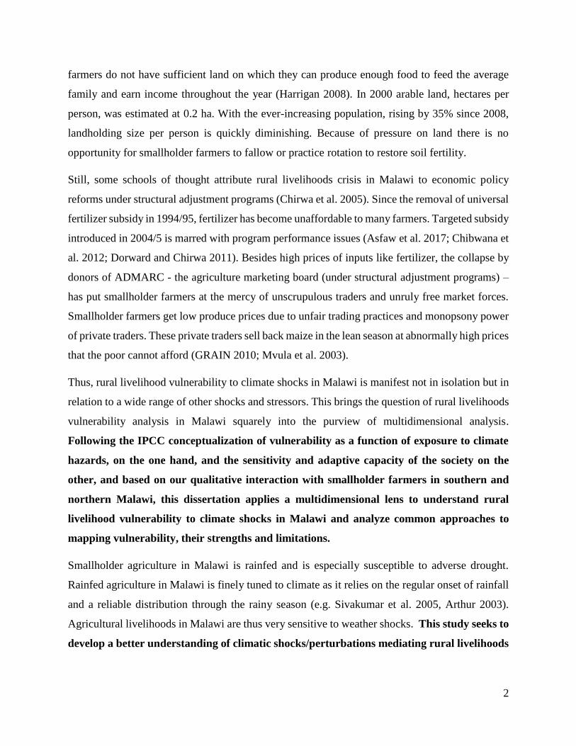
Figure 3. 4: Rainfall & Nino 3.4 time series 1961- 2012 .............................................................................. 35

Figure 3. 5: Spatial association of precipitation and El Nino phenomenon ................................................ 36

Figure 3. 6: Homogenous rainfall regions ................................................................................................... 37

Figure 3. 7: Regional rainfall and SST series ................................................................................................ 39

Figure 3. 8: May rainfall and SST series ...................................................................................................... 40

Figure 3. 9: End of rainy season and SST series .......................................................................................... 41

Figure 4. 1: Examples of vulnerability maps ............................................................................................... 46

Figure 4. 2: Studies selection criteria for the vulnerability mapping systematic review ............................ 48

Figure 4. 3: Studies by Continent, Level of Analysis, and Discipline ........................................................... 52

Figure 4. 4: Summary of the studies in terms of (a) method of spatial analysis, (b) valued attribute, and

(c) aggregation method .............................................................................................................................. 54

Figure 4. 5: Summary of the studies, clockwise from upper left, in terms of (a) timeframes of analysis

(%), (b) temporal nature of the climate parameters considered (%), (c) spatial data layers or parameters

considered (no.), and (d) climate-related phenome .................................................................................. 56

Figure 4. 6: Diagram from Kienberger et al. 2016 illustrating the elements contributing to an agricultural

vulnerability index, including weighting of the variables and components ............................................... 63

1

Chapter 1: Introduction

Since 1990s rural households in Malawi, constituting 85% of the population, have experienced

deepening livelihood vulnerability, often manifested as persistent food insecurity. For the past 15

years the government has declared a national disaster five times due to food insecurity/livelihood

failure: 2002; 2005; 2012, 2015; 2016. Livelihoods crises are also manifested in a steep increase

in food prices, which, for example, in 2002 left around 3.5 million people food insecure.

Livelihood crises have since been blamed on or attributed directly to, by government/authorities,

weather perturbations/climatic shocks i.e. El-Nino induced climate variability/drought conditions.

Others have argued/contend that the worsening repercussions of and deepening rural livelihoods

vulnerability cannot be explained by unkind weather/climatic perturbations alone. In Malawi,

smallholder farmers are not new to climate uncertainty. Over the centuries rural agricultural system

has evolved to cope with fluctuating environmental conditions. Through empirical, indigenous

knowledge, smallholder farmers have developed mechanisms, such as localized crop and varietal

diversity, to mediate livelihoods through perturbing environments. Up to 1994, Malawi was food

self-sufficient and, in many years, had surplus to export. However, these long-held coping

mechanisms have in the recent past been quickly eroded (Brooks 2014). At the intersection of

interests to promote private sector driven system, to achieve food security in the short term, and to

push hybrid seed as an appropriate technology for smallholder farmers, smallholder farming has

silently become specialized, with significant emphasis on maize production creating maize

monoculture, eroding crop and variety diversity. Overall, it is estimated that 97% of smallholder

farmers across the county grow maize, and more than half of households grow no other crops.

Only 10 % of these maize growers are net sellers, with as high as 60 % being net buyers”

(Chinsinga 2012). Maize however is not drought resistant, and to maintain yields, it requires

fertilizer and fresh hybrid seeds each year. According to Brooks (2014), specialization in

agriculture increases vulnerability to fluctuations in weather and market.

Rural livelihoods vulnerability in Malawi is further compounded by land inadequacy for

smallholder production. Malawi is densely populated, in fact is the second most densely populated

country in southern Africa (Malcomb 2014; World Bank 2018; UN 2018). Most smallholder

2

farmers do not have sufficient land on which they can produce enough food to feed the average

family and earn income throughout the year (Harrigan 2008). In 2000 arable land, hectares per

person, was estimated at 0.2 ha. With the ever-increasing population, rising by 35% since 2008,

landholding size per person is quickly diminishing. Because of pressure on land there is no

opportunity for smallholder farmers to fallow or practice rotation to restore soil fertility.

Still, some schools of thought attribute rural livelihoods crisis in Malawi to economic policy

reforms under structural adjustment programs (Chirwa et al. 2005). Since the removal of universal

fertilizer subsidy in 1994/95, fertilizer has become unaffordable to many farmers. Targeted subsidy

introduced in 2004/5 is marred with program performance issues (Asfaw et al. 2017; Chibwana et

al. 2012; Dorward and Chirwa 2011). Besides high prices of inputs like fertilizer, the collapse by

donors of ADMARC - the agriculture marketing board (under structural adjustment programs) –

has put smallholder farmers at the mercy of unscrupulous traders and unruly free market forces.

Smallholder farmers get low produce prices due to unfair trading practices and monopsony power

of private traders. These private traders sell back maize in the lean season at abnormally high prices

that the poor cannot afford (GRAIN 2010; Mvula et al. 2003).

Thus, rural livelihood vulnerability to climate shocks in Malawi is manifest not in isolation but in

relation to a wide range of other shocks and stressors. This brings the question of rural livelihoods

vulnerability analysis in Malawi squarely into the purview of multidimensional analysis.

Following the IPCC conceptualization of vulnerability as a function of exposure to climate

hazards, on the one hand, and the sensitivity and adaptive capacity of the society on the

other, and based on our qualitative interaction with smallholder farmers in southern and

northern Malawi, this dissertation applies a multidimensional lens to understand rural

livelihood vulnerability to climate shocks in Malawi and analyze common approaches to

mapping vulnerability, their strengths and limitations.

Smallholder agriculture in Malawi is rainfed and is especially susceptible to adverse drought.

Rainfed agriculture in Malawi is finely tuned to climate as it relies on the regular onset of rainfall

and a reliable distribution through the rainy season (e.g. Sivakumar et al. 2005, Arthur 2003).

Agricultural livelihoods in Malawi are thus very sensitive to weather shocks. This study seeks to

develop a better understanding of climatic shocks/perturbations mediating rural livelihoods

3

and holistic approaches (i.e. that include both climatic hazard and differential social

vulnerability) to vulnerability mapping.

A commonplace approach to holistic vulnerability analysis and mapping is to aggregate various

dimensions into a single index. This approach, however, while may be more elaborate on the

theoretical side and an improvement of the efforts that focus on exposure to natural hazard, is

marred with measurement/quantification and communication issues. On the one hand, aggregated

measures essentially reduce the multifaceted socio-ecological vulnerability to unidimensional. On

the other hand, the unitless aggregated index reduces the richness of and obscures information

regarding the original variables. Furthermore, unitless aggregated vulnerability values may return

similar scores in two locations where vulnerability is driven by very different processes - for

example, forest loss or drought (Füssel, 2009; Yohe & Tol, 2002). Besides the problem of

measurement, quantification, efforts to analyze and map vulnerability are mired by issues of data

quality. Vulnerability mapping studies traditionally rely on remotely sensed and climatological

data. Absent from these analyses are local details regarding the actual exogenous shocks reported

by households over time. In a review of 45 vulnerability mapping studies, Preston, Yuen, and

Westaway (2011) found that very few studies used actual data on exogenous shocks and

socioeconomic factors reported by households.

The question therefore persists, and we apply this question to Malawi, how can we better

understand rural livelihoods vulnerability in Malawi to leverage (to enable smallholder

farmers to effectively adapt) effective adaptation to climate change? This dissertation provides

a series of primary and secondary data analyses that examine different aspects of this question.

Livelihood adaptation to climate change literature asserts that effective adaptation to climate

change is contingent on local farmers perception (e.g. Le Dang et al 2014; Teye et al 2014;

Boissiere et al 2013). Farmers perceptions reflect local concerns and tend to form the context in

which their adaptation strategies emerge and or the conceptual framework in which farmers are

willing to accept or not adaptation strategies (e.g. Carr and McCusker 2009; Byg and Salick 2009;

Yaro 2003; Campos et al 2014).

This research thus begins in Chapter 2 with an analysis of local farmers perception of climate

change in Malawi and check the validity of local perception against meteorological observations.

It is structured as 3 closely related articles. The first article delves into actual lived experiences

4

about climate variability among local farmers to better understand environmental context i.e.

climatic conditions in which livelihood vulnerability is generated. It investigates the changing

rainfall patterns by addressing the following two questions: Is the local climate of Balaka and

Nkhata Bay changing? Are local farmers able to perceive the changes? Farmers perceptions reflect

local vulnerabilities and concerns, actual impact of climate on their livelihoods. Effective

adaptation depends on deep knowledge of vulnerability. Understanding farmers perceptions of the

changing climatic conditions is thus essential to policy makers and to adaptation research (Le Dang

et al. 2014). Teye et al. (2014) assert that effective adaptation to climate change is contingent on

the perception of farmers. Boissiere et al. (2013) also argued that knowing farmers’ perceptions of

climate change is helpful in developing strategies to support adaptation to climate change.

According to Le Dang et al. (2014) any attempt to understand adaptive behavior patterns should

come after understanding vulnerability i.e. farmers perception of climate change.

Although Malawi is heavily dependent on rainfed agricultures and is prone to rainfall variability,

very little is known about the factors governing rainfall variability i.e. variability in its climate has

not been widely studied. Known studies include Nicholson et al. (2014); Ngongondo et al. (2011);

Jury and Mwafulirwa (2002); and Jury and Gwazantini (2002). Malawi’s rainfall regime falls in a

climatic transition zone between Southern Africa and Eastern Africa. In a given year, southern

Malawi may experience different weather conditions from northern Malawi suggesting that the

rainfall regimes may be different. Thus, Malawi merits much more detailed study than regional

studies which usually report only average climatic conditions. Chapter 3 builds on earlier studies

on climate variability. It investigates the association between rainfall variability in Malawi and sea

surface temperature (SST) over the south-central Indian Ocean and Nino 3.4 time series at country

and local scales. Onset, intensity, length of the growing and rainy seasons, dry spells i.e. length of

dry spells, and their frequencies are analyzed to understand how changes in the agriculturally

relevant rainfall characteristics are associated with or mediated by SST patterns.

The dissertation research then builds on a systematic review of current practices in vulnerability

analysis and mapping to improve on ways to better analyze and map rural livelihoods vulnerability

to climate change in Malawi. Chapter 4 is a systematic review of current practices in climate

vulnerability mapping and provide recommendations that chart the way forward for future efforts.

A review of state of the art in vulnerability analysis and mapping reveals critical point/observation

5

that while studies on climate vulnerability have made valuable contribution to our understanding

of vulnerability analysis and mapping few or no studies have considered exposure to non-climatic

stressors, such as economic downturn or health crises, in addition to climatic stressors. Adopting

the framing of vulnerability, which include both climate hazard (or exposure) and differential

social vulnerability (i.e. socioeconomic characteristics affecting the susceptibility of certain

populations to climate change impacts and related risks), necessitates vulnerability mapping to

consider exposure to non-climatic stressors, such as economic downturn or health crises, in

addition to climatic stressors. Measuring and mapping vulnerability is a top research priority

(PROVIA 2013). Maps have been used to identify areas of vulnerability to climate hazards such

as flood, drought, and sea level rise (Notenbaert et al. 2010). End users have found the information

contained in vulnerability maps useful for planning adaptation assistance (de Sherbinin et al.

2017), understanding the underlying factors contributing to vulnerability (Preston et al. 2009).

Given the research and policy priority given to mapping vulnerability, it is imperative to develop

a better understanding of suitable approaches to vulnerability mapping across a range of scales,

regions, climate hazards, and thematic foci. While a number of studies have made valuable

contributions to our understanding of vulnerability mapping, there remains a need for a

comprehensive review of the state of the art in mapping social vulnerability to climate change to

chart the way forward for future efforts.

This dissertation concludes by summarizing key findings related to climatic

shocks/perturbations mediating rural livelihoods and holistic approaches to vulnerability

mapping to leverage effective adaptation to climate change. Through farmers perceptions the

study revealed that local farmers are sensitive and have detailed knowledgeable of the changing

climatic conditions in their areas. If adequately harnessed such practical knowledge of local

weather condition can facilitate effective and successful adaptation. Correlation analysis has

shown that the changing rainfall conditions over Malawi i.e. year to year variability and dry

conditions are associated with sea surface temperature (SST) i.e. the El Nino Southern Oscillation

and south-central Indian Ocean SST. The dissertation has also revealed that vulnerability mapping

as a field is maturing, but a number of issues remain that need to be addressed for the field to

advance, including increasing the degree of collaboration with end users, greater attention to map

communication, moving beyond the map as the final product, work on validation.

6

Many outcomes will result from this dissertation. Although rural livelihoods vulnerability is a

significant topic of interest in Malawi and has received widespread attention from donors, NGOs,

and the government, studies on Malawi’s rural livelihoods vulnerability are very scarce in the

literature. This dissertation will contribute to understanding local farmers environmental

conditions mediating their livelihoods and the context in which adaptation takes place. As pointed

out by Ribot (2014), there is need for a clear understanding of causes of rural livelihoods

vulnerability before adaptation. The dissertation will also directly contribute to improving

vulnerability mapping. Better and suitable approaches to vulnerability mapping can make

significant contributions to enabling society to effectively adapt, or to signal where adaptation may

face sufficiently high barriers. Thus, better understanding of geography of rural livelihood

vulnerability in Malawi can help with programming, identification of groups of people to be

targeted with adaptation interventions and monitoring progress towards adaptation.

7

Chapter 2: Has the Rainfall in Malawi Changed, and Do Farmers Perceive Change?

Abstract

Increased frequency of occurrence of weather perturbations is negatively affecting livelihoods in

southern Africa. With single season rainfed agriculture which is finely tuned to climate as it relies

on the timely onset of rainfall and its regular distribution through the rainy season, livelihoods in

Malawi are especially vulnerable to adverse weather conditions. This paper explores the lived

experiences and perceptions about weather pertubation among local farmers in Malawi. Farmers‘

perceptions reflect local concerns, thus, provide context in which adaptation strategies emerge.

Understanding farmers‘ perceptions of the changing climatic conditions is essential to policy

makers and to adaptation research. As asserted by Teye et al. (2014) effective adaptation to climate

change is contingent on the perception of farmers. Thus, perceiving climate variability is the first

and critical step in the process of adaptation. The present study uses household surveys and focus

group discussions from Balaka in southern Malawi and Nkhata Bay in northern Malawi to

investigate farmers‘ perception of the changing rainfall patterns and compare with meteorological

observations. The main findings are a) local farmers in both Balaka and Nkhata Bay are sensitive

and knowlegeable of climatic conditions in their areas and have observed that rainfall patterns

have changed; b) local farmers perceptions of climate change are consistent with meteorological

observations.

1. INTRODUCTION

While some people (particulary in the developed world) are still skeptical about climate change,

experiences of rural smallholder farmers in southern Africa, especially Malawi, attest to the saying

that the one who feels it knows it. Increased frequency of occurrence of weather perturbations is

negatively affecting livelihoods in southern Africa. As a rainfed, agro-based economy, Malawi is

especially more vulnerable to adverse conditions. Single season (November to April) rainfed

agriculture constitutes the source of livelihoods for about 85% of the population. The rainfed

agriculture in Malawi is finely tuned to climate as it relies on the timely onset of rainfall and its

regular distribution through the rainy season (e.g. Sivakumar et al. 2005, Arthur 2003). In this

8

paper, I will explore the lived experiences and perceptions about weather pertubations among local

farmers in Malawi.

In the recent past, Malawi has been experiencing frequent occurence of adverse weather conditons

which have negetively impacted livelihoods and often rendered the nation food insecure (UN-

OCHA 2016; USAID 2018). In the past 15 years, the government has declared a national disaster

four times (i.e Febreuary 2002; October 2005; January 2015; April 2016) as a result of adverse

weather conditions. Enhancing and broadening our understanding of the temporality of rainfall in

Malawi is thus central to improving/supporting peoples livelihoods.

Although climate and rainfall variability is a significant topic of interest in Malawi and has

received widespread attention from donors, NGOs, and the government, studies on Malawi’s

rainfall are very scarce in the literature. While Ngondondo et al. (2011) investigated the spatial

and temporal rainfal patterns and Nicholson et al. (2014) analysed the interannual rainfall

variability, few attempts have been made to understand the actual lived experiences and

perceptions about climate variability among local farmers at local level in Malawi.

As the literature on farmers perceptions on climate change has matured, the validity/accuracy of

the peceptions has been debated. Panda (2016) observed that there is a dearth of concrete findings

that link between farmers‘ perception on changing climate and meteorological data. Literature on

farmers‘ pereceptions has also higlighted the importance of percetions about climate change on

farmers‘ adaptation actions. Deressa et al. (2011) found that in Ethiopia, farmers that perceived

decreasing rainfall undertook adaptation actions. According to Ogalleh et al (2012), farmers use

their perceptions to make decisions on coping and adapting. Since farmers perceptions reflect local

concerns, farmers perceptions of climate change tend to form the context in which adaptation

strategies emerge or the conceptual framework in which farmers are or are not willing to accept

adaptation strategies (e.g. Byg and Salick 2009; Yaro 2013; Campos et at. 2014).

Understanding farmers‘ perceptions of the changing climatic conditions is essential to policy

makers and to adaptation research (Le Dang et al. 2014). Studies on farmers perception enable

policy makers to design relevant policies as they understand what farmers adapt to. As asserted by

Teye et al. (2014) effective adaptation to climate change is contingent on the perception of

farmers. Boissiere et al. (2013) also argued that knowing how farmers perceive climate change is

9

helpful in developing strategies to support adaptation to climate change. According to Le Dang et

al. (2014), any attempt to understand adaptive behaviour patterns should come after understanding

how climate variability is perceived by farmers. Thus, perceiving climate varibility is the first and

critical step in the process of adaptation.

The present study, using household surveys, focus group discussions and meteorological

observations from Balaka in southern Malawi and Nkhata Bay in northern Malawi, investigates

the changing rainfall patterns at local level. The main findings are a) local farmers in both Balaka

and Nkhata Bay are sensitive and knowlegeable of climatic conditions in their areas and have

observed that rainfall patterns have changed; b) local farmers perceptions of climate change are

consistent with meteorological observations. These two areas make ideal case studies for studying

changing rainfall patterns and farmers‘ perceptions because they are suitable for comparison as

they represent geographies with contrasting natural environment conditions and social-cultural and

livelihood system, this study zeroes in on the following specific questions: is the local climate of

Balaka and Nkhata Bay changing? Do the local farmers perceive the changes? Given that Malawi

has been exposed to frequent adverse climatic conditions and that understanding of climate

variability remains limited, this study will be useful in understanding the rainfall pattern, and in

achieving effective adaptation to climate change in Malawi. The rest of the paper is organized as

follows. Section 2, lays out the context for the study by describing the study area, data sources,

and data analysis methods used in the study. Section 3 presents results and discussion and discusses

how smallholder farmers perceive climatic changes that have occurred for the past 46 years against

meteorological observations. Section 4 briefly concludes the study.

2. STUDY AREA

The study is situated within the context of Malawi (latitudes 9–17°S and longitudes 32–36°E), in

southern Africa. Malawi is landlocked bordered by Mozambique, Zambia and Tanzania. With a

total area of 118,484 km² (29,604 km² of which is water, mainly Lake Malawi) and an estimated

population of 18 million (2016), Malawi is the most densely populated country in southern Africa.

It experiences semi-arid tropical wet and dry climate, also called savanna. The rainy season is from

November to April and the dry season is from May to October. Mean annual rainfall is in the order

of 800 mm to over 1600 mm (Nicholson et al. 2014). The average daily minimum and maximum

temperatures in November, the hottest month, are 17oC and 29oC respectively; those in July, the

10

coolest month, are 7oC and 23oC. Due to variations in altitudes there are wide differences in climate

across the country. According to Ngongondo et al. (2011) the climate of Malawi is mostly

influenced by the north-south migration of the intertropical convergence zone (ITCZ) and its

topography. Rainfall is erratic, floods and droughts occur more often.

The economy is undiversified and highly dependent on rain-fed agriculture. Agriculture accounts

for more than 30% of Growth Domestic Product (GDP), 85% of the labor force and 83% of foreign

exchange earnings. Agricultural production is predominantly smallholder and subsistent,

characterized by low levels of input and output. Smallholder farmers produce about 80 percent of

Malawi’s food. The main agricultural products grown by smallholder farmers are maize, tobacco,

cassava, groundnuts, pulses, sorghum and millet, rice, bananas, sweet potatoes and cotton.

Livestock accounts for less than 7% of the agricultural GDP in Malawi. Only 4% of the households

own cattle. A tiny fraction, about 2.3% of arable land is irrigated. And only around 3.3 percent of

all rural households are beneficiaries of the irrigation schemes. Given the lack of irrigative

infrastructure agriculture is highly dependent on suitable weather conditions and is thus

particularly highly vulnerable to weather shocks such that success of crop production is almost

entirely linked with weather conditions.

As in most of southern Africa, rural livelihoods in Malawi depend heavily but not solely on rain-

fed agriculture. At the intersection of interests to promote private sector driven system, to achieve

food security in the short term, and to push hybrid seed as an appropriate technology for

smallholder farmers, the once diversified smallholder farming has gradually become specialized,

with significant emphasis on maize. Estimates show that maize farming covers more than 70% of

the arable land (GoM, 2006). And according to Chinsinga et al. (2012) an estimated 97 % of

smallholder farmers across the county grow maize, and more than half of households grow no

other crops. Maize monoculture agricultural system has made rural livelihoods fragile and more

vulnerable to weather perturbations. Cassava production is relatively high in Karonga and Nkhata

Bay districts in the northern region. With comparatively low requirement for water, labor, and

inputs, cassava helps smallholder farmers ensure local food security in the event of maize crop

failure and maize price increases. Most smallholder farmers draw their income from sale of crops

mainly tobacco, cotton, and also food crops. The market for the two major cash crops, tobacco and

cotton, is unpredictable and is affected by international factors beyond the country’s control. On

11

the other hand, the market for crops is mainly in the country’s urban centers, so is predictable and

is relatively stronger in the south and center than in the north. Supply however, tends to exceed

demand everywhere and farmers returns are therefore generally very low. Consequently, rural

household incomes are very low. Rural households also draw income from off-farm sources of

casual labor (ganyu), sale of firewood, charcoal, and from migrant remittances from family

members working elsewhere. In the lakeshore areas especially, southern region rural households

generate income from fishing, including fishing ‘ganyu’ and fish trading. In the Shire Highlands

especially the Thyolo-Mulanje Tea Estate area, most households are estate workers.

Two case study sites were selected, Balaka in the south and Nkhata Bay in the north, to explore

and gain insight into actual lived experiences and local perception about the weather perturbations.

These two study areas were purposively selected because they represent geographies with

contrasting natural environment (biophysical conditions), livelihood systems and cultural and

socioeconomic characteristics. They are ideal case studies for exploring climate variability as they

epitomize a range of socio-ecological environments applicable to most parts of Malawi.

12

Figure 2. 1: Study districts

Nkhata Bay is located in the northern region of Malawi. It is characterized by high rainfall and

rocky soils and comprises an escarpment leading down from the Viphya Mountains to the

lakeshore. The average annual rainfall is 1598mm. The average temperature is between 23.5oC.

Besides having a fairly moist climate; rainfall is also spread out over a longer period than in other

parts of the country. With high rainfall but poor soils, cassava is the dominant crop in the area.

Other crops grown in the area include maize, sweet potatoes, rice, and bananas. Animal traction

and livestock production are also limited. Local livelihoods vary according to ecological factors,

i.e. topography and ecosystems in which the communities are located. Those along the lake are

engaged primarily in fishing. Fishing is undertaken throughout the year, but peaks from mid-

November to March following the rains. Generally, the area is described as ‘food-rich’ but ‘cash-

poor.’ Like most parts of the northern region, Nkhata Bay area is largely rural (not urbanized) and

commercially isolated with poor road network and there are limited markets for the agricultural

produce. There are few sources of income available besides the sale of crops.

13

On the other hand, Balaka is located in the southern region of Malawi. It has a relatively dry climate

and is ecologically fragile and susceptible to frequent droughts. The average annual rainfall is

971mm. The average temperature in Balaka is 23.1oC. The area is characterized by near-

subsistence farming, with fishing on a small scale amongst those living close to the Shire River.

Crop production is relatively low due to agricultural droughts. The main crops include cotton,

maize, and sweet potatoes. Unlike Nkhata Bay, Balaka is highly populated and connected to

markets in the country's region with biggest urban population as well as its largest commercial

sector. The ‘poor’ households earn income through ganyu, petty trade, firewood and charcoal

burning and other collection-activities, feeding the market in the southern region’s urban centers.

Market prices of staple food vary seasonally. Prices are lowest during the harvesting period and

highest during the ‘hunger’ season, which is between December and February. Most local markets

are managed by private traders (i.e. following liberalization).

Based on our knowledge of the study districts through in-depth interviews in the localities we

identified 3 communities in each study area. The communities were purposively selected to ensure

adequate representation of the study districts. We then randomly selected households in each

community.

3. DATA COLLECTION

A mixed methods approach was used to collect data. To draw on their complementarities, we

conducted quantitative household surveys and also focus group discussions to explore and explain

survey results. Six communities, three in Balaka and three in Nkhata Bay, were purposively

selected to gather data on local farmers’ perceptions about weather perturbations. In order to ensure

adequate representation and minimize idiosyncrasies, study communities were selected to include

all different socio-economic as well as biophysical characteristics. A systematic sampling

technique was used within the communities to select the households. The survey was designed to

include both male and female headed households. The heads of household were interviewed. If the

household had the father and mother around, both were interviewed. A total of 515 households

participated in the surveys. In the Nkhata Bay 298 households were interviewed: 103 females and

193 males. In Balaka 217 households were interviewed: 88 females and 129 males. The interviews

were conducted by trained field assistants in the local languages of Tumbuka in the north and

Chichewa in the south by trained field assistants.

14

A total of 20 focus group discussions were conducted to gain deeper insights into farmers’

perception regarding climate conditions. The focus group discussions included people of different

social status i.e. traditional leaders and ordinary men and women, young and elderly, natives and

immigrants to capture the different perceptions. The number of participants in each focus group

discussion (FGD) ranged from 8 to 14. A total of 244 participated in the focus group

discussions:106 males and 138 males. A discussion guide was used to facilitate and moderate the

discussions which generally took about two-three hours.

The climatological data used in this study was obtained from the Malawi Department of Climate

change and Meteorological Service. It included the continuous 46 years (i.e. for the period between

1970 and 2016) monthly and daily rainfall observations collected from Balaka and Nkhata Bay

meteorological stations. Quality control of the data was largely carried out by the Malawi

Department of Climate change and Meteorological Service. However, we noticed about 5

randomly missing entries in the daily rainfall data for Nkhata Bay which were reported as blanks.

We applied the more flexible methods of group mean and regression to replace the missing entries.

The two methods gave almost similar values for the missing entries.

4. DATA ANALYSIS

Data analysis was conducted to compare and validate farmers perceptions with meteorological

observations, looking for agreement or disagreement. Exploratory and summary statistics were

used to explore and analyze quantitative (household survey) data on perceptions of farmers on

climate variability and change. Qualitative data was analyzed thematically. The transcribed

discussions were rigorously coded, ordered and structured into specific themes. Key themes

included among others: irregular timing and distribution of rainfall - change of the rainfall

calendar, in which the rains start late and end early, frequent occurrence of dry spell, rains not

coming at the right stage of crop production; reduced amount of rainfall; increased occurrence of

lightning and thunderstorms; and increasing temperature.

Qualitative data was analyzed thematically. Through an iterative process, transcribed focus group

discussions were explored, queried, visualized, and coded in NVivo 12. Word frequency query

was conducted as preliminary analysis to get an overview of the discussions highlighted rains;

15

changes; timing – start, end, early, late; planting; heavy, severe intensity - as most occurring

themes, as displayed in the Word Cloud below.

Figure 2. 2: Word cloud

These were then coded into specific themes which included: timing of rainfall; distribution of

rainfall; change of planting/farming calendar; changes in the amount of rainfall; occurrence of

extreme event; impact on farming activities among others.

Climatological data analysis involved the use of normalized precipitation anomaly series and

Mann-Kendall test to understand temporal rainfall characteristics. The normalized rainfall

anomaly series were used to assess inter-seasonal and annual rainfall variability. Mann–Kendall

(MK) test was used to assess temporal trends in rainfall data (meteorological observations) at

annual, seasonal, monthly and daily scales. MK is a non-parametric test, which is robust,

insensitive to missing data and outliers and is recommended by World Meteorological

Organization (WMO) for trend analysis in meteorological data (e.g. Ngongondo et al. 2011; WMO

1988). Several studies have employed MK to assess trends in rainfall and temperature data (e.g.

Taylor and Loftis 1989; Yu et al. 1993; Xiong and Guo 2004; Basistha et al. 2009). MK was

complemented with Sen’s slope estimation to quantify the slope of the trends.

The acf () and pacf () functions in R, which compute the autocorrelation and partial autocorrelation

corresponding to the time series, were used to visually investigate the presence of serial correlation

16

among the annual, seasonal, monthly and daily precipitation levels. Inspection of the serial

correlation was conducted prior to applying Mann-Kendall test to ensure that the right measures

are taken, specifically to use Mann-Kendal test in conjunction with bootstrapping in the case of

the presence of significant serial correlation to correct for the P-value of the test for serial

correlation.

5. RESULTS

5.1. Climate change and variability: farmers’ perception

Although farmers from both locations i.e. Balaka and Nkhata Bay had difficulties defining the

term “climate change”, the household surveys and the focused group discussions showed that the

they are more aware and sensitive to the changes in rainfall patterns that have occurred in their

areas affecting their livelihoods when the term “rainfall changes” is used in questions. The

household surveys show that almost all the surveyed smallholder farmers from both locations have

observed changes in climatic conditions particularly rainfall. In Balaka, 208 (96%) households

indicated that rainfall has changed. In Nkhata Bay, a large share of households 290 (97%) also

reported that rainfall has changed.

Despite the geographic, biophysical, and social-cultural context differences between the regions,

the farmers perceptions of the changing climatic conditions were comparable in the two case

studies. In Balaka many smallholder farmers, about 41% observed that compared to the past

rainfall has become more erratic meaning there is no predictable and reliable rainfall calendar any

more. “In the past”, farmers observed, “rains used to begin and fall consistently, now there are

frequent and extended dry spells”. This was followed by perceptions that the rainy season has

shortened or reduced (i.e. 18%), and that there is a late onset of rainfall (13%), and that rainfall

events were oftentimes more intense (12%). Farmers reported that rainfall used to start in October

and fall through to May. Unlike the past when they could grow two crops in a season as the season

was long, now the rain ends well before crops mature. A small number (8%) reported that rainfall

has decreased. In Nkhata Bay a large number of smallholder farmers (31%) perceived that rainfall

is often intense and associated with strong winds, lightning and thunder. This was followed by

perceptions that the rainfall was erratic (25%), and that rainy season has shortened (17%), and that

rainfall start late (11%). A considerable number (7%) also reported that rainfall has decreased

17

(Figures 2.3 and 2.4). To a large extent men and women stressed similar concerns about the

changing rainfall patterns.

Figure 2. 3: Weather Changes observed,

Nkhata Bay

Figure 2. 4: Weather Changes observed,

Balaka

Through focused group discussions smallholder farmers were able to expound on their actual lived

experiences with regard to their perceptions about climate change. In the focused group

discussions, farmers explained that they used to receive regular and reliable seasonal rainfall – the

right amount of rainfall and on time. They mentioned that in the past rainfall would start in October

or early November and they would plant by November, but now rains start in December. In Kavuzi,

Nkhata Bay, for example, one farmer highlighted:

“It used to be that the very early rains called ‘chicocola nyoni’ would fall in June

and July, and then by mid-October we would receive the first rains locally called

‘chizimya lupya’. The main rains called ‘kuoloka’ would fall from November to

January; In March and April we would have heavy rains called ‘zandi’ and the

rivers would also flood.” [old man].

Farmers further emphasized that the rainy season was shorter now and the frequency of dry spells

has increased. Farmers explained that they used to have rains starting after mid-October through

to late April or early May which would amply support more than one crop in a season. Nowadays,

the rainy season is short, rain start in December, often punctuated with severe dry spells and ends

0 10 20 30 40

Intense

Short rain season

decreased

No change

Percent

Local perceptions about rainfall, Nkhata Bay

0 10 20 30 40 50

ErraticShort rain season

Late onsetIntense

GoodDecreasedNo change

Percent

Local perceptions about rainfall, Balaka

18

early March. One older man in Mpamba, Nkhata Bay cited the dry spell that occurred in the

2014/2015 season as an example:

“This rainy season we had first rains on the 16th of October, so we planted because

we are used to planting with early rains and we are also advised by agricultural

extension officer to plant early. But then there were no rains up to the 21st

December and the temperature was very high in between” [very old man].

Farmers mentioned that the reduced amount but also the irregular timing and distribution of rainfall

is negatively affecting their farming activities. One woman lamented: ‘even when the rain come,

it does not help us as it does not come at right stages of crop production, particularly maize crop.’

Some farmers complained about incessant rainfall at harvest time, when they expect no rain, which

destroy the little crop that managed to mature.

Farmers, further, commented that unlike in the past when they used to have proper amount of rain,

almost every month in the rainy season now the rains are unpredictable. Often when they are

expecting rain, they instead experience lightning and thunder and very strong winds that blow the

clouds away, which stops the rains. In Sanga, Nkhata bay (along Lake Malawi) the locals

mentioned that frequent occurrence of strong winds over the lake in the rainy season negatively

affects their fishing livelihoods.

Apart from changing rainfall patterns farmers also mentioned about increasing temperature.

Farmers in Mpamba, Nkhata Bay, for example, recounted :

‘We were blessed with good climate here in Mpamba, it used to be cool in the winter

months, but it is no longer the same, temperatures get very high all year round such that

we don't even sleep with a bedsheet’.

5.2. Climate change and variability: meteorological observations

Results of the analysis of the monthly mean rainfall (for the period 1970 – 2016) reveal that there

are differences in the distribution of rainfall between the two study sites. In Balaka, rainfall is

concentrated in the months of November to March. The peak rainfall occurs in January. In Nkhata

Bay, on the other hand, rainfall is spread in the months of November to May, with maximum

rainfall occurring in March. Nicholson et al. (2014) in their study of mean rainfall climatology of

Malawi also observed similar patterns that along the northern lakeshore region maximum rainfall

19

occurs in March, and it is one of the wettest parts of the country with the longest rainy season. For

the southern regions, they also observed that peak rainfall occurs in January. Mean rainfall analysis

also revealed high year to year rainfall variability for both locations, Balaka and Nkhata Bay

(Figures 2.5; 2.6; 2.7; & 2.8).

20

Figure 2. 5: Monthly rainfall, Balaka

Figure 2. 6: Annual rainfall, Balaka

Figure 2. 7: Monthly rainfall, Nkhata Bay

Figure 2. 8: Annual rainfall, Nkhata Bay

The results of MK test on rainfall series in Balaka show that rainfall has decreased over the period

1970 – 2015 (see Table 1 below). Annual and seasonal (November through April) rainfall series

demonstrates significant decreasing annual and seasonal rainfall trends at average rates of -5.8mm

/year and -5.9 mm/season, respectively. Monthly analysis of seasonal rainfall series (not shown

here) shows significant downward trends in November, December, February, March, and April at

average rates of -1.1, -2.0, -1.7, -1.7 and -0.7, respectively. Only the month of January

demonstrated a positive trend, but it was not statistically significant. Daily analysis of the rainfall

series also demonstrates statistically significant decreasing trends in the number of rain days

0.050.0

100.0150.0200.0250.0

JUL.

AU

G.

SEP

.O

CT.

NO

V.

DEC

.JA

N.

FEB

.M

AR

.

AP

R.

MA

YJU

N.

Rai

nfa

ll in

mm

Month

Mean Monthly Rainfall in Balaka, 1970-2015

0.0

500.0

1000.0

1500.0

19

70

19

75

19

80

19

85

19

90

19

95

20

00

20

05

20

10

20

15

Rai

nfa

ll in

mm

Year

Annual Rainfall in Balaka, 1970-2015

0100200300400

JUL.

AU

G.

SEP

.

OC

T.

NO

V.

DEC

.

JAN

.

FEB

.

MA

R.

AP

R.

MA

Y

JUN

.Rai

nfa

ll in

mm

Month

Mean Monthly Rainfall in Nkhata Bay, 1970-2015

0

500

1000

1500

2000

2500

3000

19

70

19

73

19

76

19

79

19

82

19

85

19

88

19

91

19

94

19

97

20

00

20

03

20

06

20

09

20

12

20

15

Rai

nfa

ll in

mm

Year

Annual Rainfall in Nkhata Bay, 1970-2015

21

annually and seasonally as well as for the months of November, March, December (marginal) and

April (marginal) (not shown here).

Statistical analysis of meteorological data from Nkhata Bay also reveal decreasing trend in

precipitation between 1970 and 2015. Annual and seasonal (November through April) rainfall

series demonstrates decreasing annual and seasonal rainfall trends at average rates of -1.8mm/year

and -1.3 mm/season), respectively. While the annual and seasonal rainfall series show decreasing

trends, this downward trend is not statistically significant at 5% level. Statistically significant

decreasing trend, however, is demonstrated for the monthly analysis of seasonal rainfall series for

December, March and May (marginal) at average rates of -2.4, -2.98, and -1.3, respectively. The

month of March also revealed a significant decreasing trend in the magnitude of rain events.

Statistically significant decreasing trends in number of rain days were demonstrated for the month

of April.

Table 2.1: Trends in the Annual and Seasonal Rainfall

Study site Annual/Seasonal MK P value Sen’s slope

Balaka

1970 - 2015

Annual -0.233 0.023* -5.756

Seasonal (November - April) -0.233 0.023* -5.896

Nkhata Bay

1970 - 2015

Annual -0.044 0.677 -1.781

Seasonal (November - April) -0.037 0.712 -1.281

* Significant at 5% level

In order to get an overview of the start and end of rainy season from the meteorological

observations, the definitions of onset and end of a rainy season by Tadross et al. (2009) were

followed. According to Tadross et al. (2009) the onset of a rainy season is once 25mm of rainfall

has accumulated within 10d, without 10 consecutive dry days (< 2 mm) occurring afterward. The

end of a rainy season is defined as 3 consecutive dekads (after February 1) of < 20 mm each. The

statistical analysis of the meteorological daily rainfall observation between 1970 and 2015

demonstrates that onset and end of the rainy season in Balaka and Nkhata Bay have shifted. Figures

22

2.9; 2.10; 2.11; & 2.12 show an increasing trend in the number of days between actual day of onset

and the expected date of onset (i.e. after mid-October) and decreasing trend in the number of days

between 1st February and the end date of the rainy season for both locations, Balaka and Nkhata

Bay. The changes however are statistically significantly only in Balaka and not in Nkhata Bay.

Figure 2. 9: Onset of rainy season, Balaka

Figure 2. 10: End of rainy season Balaka

Figure 2. 11: Onset rainy season, Nkhata Bay

Figure 2. 12: End of rainy season, Nkhata

Bay

y = 0.873x + 41.304

0

20

40

60

80

100

120

19

76

19

79

19

82

19

85

19

88

19

91

19

94

19

97

20

00

20

03

20

06

20

09

20

12

20

15

Nu

mb

er o

f d

ays

Year

Number of days between the expected and actual onset of the rainy season, Balaka

y = -0.873x + 66.696

0

20

40

60

80

100

120

19

76

19

79

19

82

19

85

19

88

19

91

19

94

19

97

20

00

20

03

20

06

20

09

20

12

20

15

Nu

mb

er o

f d

ays

Year

Number of days between the 1st February and end date of the rainy season, Balaka

y = 0.1685x + 42.213

0

20

40

60

80

100

19

70

19

74

19

78

19

82

19

86

19

90

19

94

19

98

20

02

20

06

20

10

20

14

Nu

mb

er o

f d

ays

Year

Number of days between the expected and actual onset of the rainy season, Nkhata Bay

y = -0.4382x + 125.26

0

50

100

150

200

19

70

19

74

19

78

19

82

19

86

19

90

19

94

19

98

20

02

20

06

20

10

20

14

Nu

mb

er o

f d

ays

Year

Number of days between the 1st February and end date of the rainy season, Nkhata Bay

23

5.3. Climate change and variability: perception & meteorological observations

Farmers’ perceptions about climate variability and change had been considered less reliable (e.g.

Held et al. 2005, Weber 2010). This assertion has been consolidated by studies that have found

inconsistencies between local perceptions and meteorological data and questioned the validity of

local perceptions (e.g. Hansen et al. 2004; Sanchez-Cortes and Chavero 2011; Sivakumar et al.

2005; Maddison 2006; Van Aalst et al. 2008; Ovuka and Lindqvist 2000), however, this is in sharp

contrast to the results of our study. The results of our study illustrate that local farmers are sensitive

and aware of the changes in the climatic conditions occurring in their areas.

Our study supports observations that local farmers are knowledgeable of the changes in the

climatic conditions occurring in their areas. The results of our study show that local farmers’

perceptions about rainfall variability and change in Balaka and Nkhata Bay are comparable with

the meteorological observations. Farmers perceptions that rainfall has decreased closely

corroborate with actual rainfall data from Department of Climate Change and Meteorological

Services, which show a decreasing trend in precipitation between 1970-2016. Our findings of

downward trend in precipitation resonates with the trends established by Ngongondo et al. (2011).

Ngongondo et al. (2011) analyzing the temporal rainfall pattern for Malawi also observed

decreasing trend in precipitation. Consistent with meteorological observations local farmers also

correctly perceived that the rainfall pattern has changed such that the rainy season has shortened

with rains starting late and ending early so the number of days in the rainy season have decreased.

Furthermore, in line with farmers perceptions statistical analysis (SPI) of actual rainfall data show

that frequency of dry spells in the rainy season have also increased over the period 1970-2016,

with the increase mostly after 1990.

While statistical analysis demonstrates that all the observed change in precipitation are statistically

significant at 95% level for Balaka, not all observed changes in precipitation are statistically

significant in Nkhata Bay at 95% level. Farmers, perceptions of decreased precipitation might have

been influenced dominantly by the statistically significant downward rainfall trend for the month

of December. For the most part local farmers in the north plant their crops in December and

24

bearing in mind that planting is tied to adequate rainfall, it is not surprising that local farmers

interpreted the rainfall changes that have occurred in December as decreasing seasonal or annual

rainfall. A significant decline of rainfall in March might have also influenced farmers’ perceptions.

As observed earlier, and also as established by Nicholson et al. (2014), March is the month when

seasonal rainfall is at its peak in Nkhata Bay. Failure to see river flooding or at least flowing to

their full capacity made farmers to perceive that rainfall has decreased.

The consistency of local perceptions with meteorological observation sturdily demonstrates that

local perceptions about climatic conditions are reliable and valid. For centuries, from generation

to generation, small holder farmers in Malawi have mainly depended on rainfall for their

livelihoods. Farmers have, over the years, developed in-depth knowledge of their local climatic

conditions, no wonder they are able to correctly notice changes in rainfall taking place in their

areas. The results of our study thus agree with Maddison (1996), who also argued that people who

depend on rainfall for their livelihoods are more likely to notice changes in climatic conditions.

With low coverage (low network of rain gauges) meteorological stations, local perceptions serve,

in many areas, as the only detailed source of information about climate variability change.

Furthermore, together meteorological observation and local perceptions can provide more valuable

insights.

Even though climate change is bringing climatic conditions beyond what local farmers have

experienced in the past i.e. past climate perturbations, local farmers usually draw from their

knowledge and perceptions to respond to climate shocks. As pointed out by Boissiere et al. (2013)

farmers use local knowledge to interpret and respond to environmental perturbations. External

intervention for facilitating local adaptation to climate change in Balaka and Nkhata Bay thus are

more likely to be successful if they build on this existing knowledge of rainfall by the locals. Local

knowledge can be useful for designing policy for dealing with impact of climate change. The

strategies and initiatives to support local adaptation should be tailored according to local

perception. With better and deeper understanding of local situations the local players (traditional

leaders and politicians), government departments, as well as international organizations and civil

society could be more effective and better leveraged to mediate local interventions, including rural

livelihood coping and adaptation strategies, safety net programming, and food security and policy

formulation. In essence, local knowledge is central to shifting from the usual and dominant

25

unrealistic and palliative “top-down” perspective and measures driven by global climatic model

scenarios to working from the “bottom-up”.

6. SUMMARY AND CONCLUSION

This study attempted to examine farmers’ perceptions of changes in precipitation and compared

them with meteorological rainfall observations. The analysis aimed to assess if rainfall in the study

areas is changing and if farmers are able to perceive the changes correctly. The study revealed that

almost all the farmers in both locations, Balaka and Nkhata Bay are sensitive and knowledgeable

of the climatic conditions in their areas and observed that rainfall has changed. Although local

farmers did not have written records but rather based their perceptions on experience, when

perceptions were compared with meteorological observations, the analysis indicated that what

local farmers observed in both locations was consistent with meteorological observations. In

Nkhata Bay it seems farmers perception of declining rainfall was largely shaped and influenced

by changes observed in rainfall amount in December when they expect to plant their crops and

March when they expect rivers to flood. The correctness at which local farmers perceived the

changes in rainfall sturdily support the assertion that local perception of climate change is reliable

and consistent with meteorological observations.

Local farmers provided more detailed information about changes in climatic conditions especially

rainfall in their areas. We posit policy makers can and should harness such detailed, extensive, and

correct knowledge of local weather condition that local farmers possess to facilitate effective and

successful adaptation. To ricochet the arguments raised before (at the beginning), policies or

initiatives and strategies that are tailored on local perceptions are more accepted. Local farmers

react to change that they observe, adaptation strategies must be specific t locations needs. Thus,

while climate change is global, adaptation policies and initiatives or strategies that are not tailored

to local need are likely to flop. Building adaptation programs on local perceptions ensure local

agreement and participation. Since local perceptions are an essential component of a local

response, it is our recommendation that policy makers tap into local perceptions across the country

such as unearthed in this study in order to facilitate and achieve sustainable and successful

adaptation to climate change.

26

Chapter 3: The Variability of Rainfall in Malawi and its Links to Sea-Surface

Temperatures (SSTs): Case of Nkhata Bay.

Abstract

Year to year variability of Malawi rainfall and its possible association with sea surface temperature

(SST) i.e. the El Nino Southern Oscillation (ENSO) and south-central Indian Ocean SST is

investigated. Correlation analysis is employed to diagnose the link between annual/seasonal and

monthly variability of precipitation over Malawi and Nino 3.4 index and south-central Indian

Ocean SST for the period 1961-2012. Results show that anomalously warm SST over the south-

eastern Indian Ocean and the tropical Pacific Ocean, typical of El Nino conditions, is associated

with dry conditions over a greater part of Malawi. The association between ENSO and occurrence

of dry conditions in Malawi however is not uniform, both spatially and temporally; in some cases,

there is a strong correlation, and other cases show moderate to no association, or the reverse. A

relatively strong positive correlation between rainfall and Nino 3.4 SST is observed in the northern

part of Malawi close to Tanzania and negative values are observed in the central and southern part

of the county. In some parts of there is a recognizable negative association between rainfall

variability at seasonal and monthly time scales, with south-eastern Indian Ocean SST time series

after 1980.

1.0 INTRODUCTION

Climate change is one of the major environmental issues affecting southern Africa. Studies

indicate that southern Africa is warming at range from 0.2 oC to more than 0.5 oC per decade

(Hulme et al., 2001). The warming is accompanied by extensive changes in precipitation. Jenkinsi

et al (2002) observed that rainfall has reduced substantially over the last 60 years. Available

projections suggest that southern Africa, in general, will experience drier and more extreme

conditions and increased frequency of drought (Wang 2005; Moise and Hudson 2008; Shefield

and Wood 2008). In recent past, for example, different parts of southern Africa have been affected

by devastating floods and severe droughts. There were devastating floods in 2015 and 2001in

southern Malawi and in southern Mozambique respectively and also more recently, in 2019.

Severe droughts occurred 2015/16, 2003/4, 2002/3, and 1991/2 across the region. In some part of

the region i.e. over parts of Botswana and Zimbabwe rainfall rates have declined, with decreases

27

of more than 0.4 mm day−1 (Hulme (1992). According Funk et al. (2008) the region is also

experiencing a decrease in growing-season rainfall since 1980s.

Looming climate change is a serious threat to people’s livelihoods in southern Africa as rain-fed

agriculture constitutes a major source of livelihoods in the region (Arthur 2003). Agriculture in

the region is finely tuned to climate, dependent on the timely onset of rainfall and its regular

distribution through the rainy season. Even a slow, small change towards a worsening climate can

increase climatic risks (Sivakumar et al. 2005, 53) on crop and livestock production. Changing

climatic conditions are also associated with increased risk of livestock stress and diseases, and

crop pests and diseases. For commercial crops, extreme events such as cyclones, droughts and

floods lead to larger damages than only changes of mean climate (Zhao et al. 2005). Climate

change is also negatively impacting on economies in the region, in 1992 for example drought

reduced the GDP of Zimbabwe and Zambia by 8–9% (Benson and Clay 1998).

Studies associated rainfall variability in southern Africa with changing SST patterns in the

Equatorial Pacific and Indian Oceans (e.g. Nash and Enfield 2008; Cook et al. 2004; Allan et al.

2003; Mason 1995; Walker 1990; Lindesay 1988; Rocha and Simmonds 1997; Funk et al. 2008;

and Chan et al. 2008; Van Loon and Shea, 1985; Nicholson and Entekhabi, 1986; Ropelewslu and

Halpert, 1987, 1989; Janowiak, 1988). Lindesay (1988), for example, associates around 20% of

the variance in late austral summer rainfall in the region with the Southern Oscillation Index.

Usman and Reason (2004) also observed that there is a coherent and marked relationship between

occurrence of dry spells and Nino 3.4 sea surface temperature (SST) anomalies. Rocha and

Simmonds (1997); Funk et al. (2008); and Chan et al. 2008) have observed that, anomalously warm

SST in the central Indian Ocean, which are partially independent of ENSO, dominate the rainfall

response in southern Africa. According to Rocha and Simmonds (1997) and also Funk et al. (2008)

rainfall deficit over Southern Africa is as a result of the SST warming in the central Indian Ocean,

which sets up cyclonic low-level circulation anomalies over the ocean.

Although vulnerability to climate variability and extreme climate events is a major concern for

southern Africa, efforts to understand climate variability and change are relatively sparse relative

to other parts of the world (e.g. Desanker and Justice 2001; Sivakumar et al. 2005). Efforts to

understand rainfall variability have mainly focused on regional studies. Little to no comparable

knowledge exists at local or country scale regarding rainfall variability. Due to high spatial and

28

temporal heterogeneity of rainfall over southern Africa (more heterogeneous than any other

regions of the world), regional based studies or regional mean rainfall condition are less useful and

applicable to agricultural livelihood activities. For many parts of southern Africa, changes in the

mean rainfall vary on relatively small spatial scales and sometimes give rise to endemic droughts

(Shongwe et al. 2009), countries face sometimes both floods and drought in different parts in a

given year (Jury et al. 2006).

Thus, more focused rainfall studies are necessary to complement the regional studies and provide

a more comprehensive understanding of rainfall characteristics. This is particularly essential for

countries such as Malawi with an economy that is agriculturally based, and with agriculture that

is predominantly rainfed (i.e. about 90%). Single rainy season – (November to April) - rainfed

subsistence agriculture constitutes almost the only source of livelihoods for about 85% of the

population. With rainfed agriculture that is finely tuned to climate, increased frequency of

occurrence of weather perturbations is negatively affecting people’s livelihoods and the economy

in general. Since 2000, Malawi has more than four times experienced livelihood failure in the form

of a national food shortage. In 2015, floods and heavy rainfall affected about one million people,

destroyed crops and property. Poor rains during 2015–2018 reduced water levels in the Shire River

negatively affecting generation of electricity, causing serious power shortages with severe impacts

on the economy. An understanding of rainfall at finer temporal and spatial resolution would more

effectively contribute to a better understanding of rainfall variability and more useful for and

applicable to smallholder farmers’ adaptation needs.

Although Malawi is heavily dependent on rainfed agricultures and is prone to rainfall variability,

very little is known about the factors governing rainfall variability i.e. variability in its climate has

not been widely studied. Known studies include Nicholson et al. (2014); Ngongondo et al. (2011);

Jury and Mwafulirwa (2002); and Jury and Gwazantini (2002). Malawi’s rainfall regime falls in a

climatic transition zone between Southern Africa and Eastern Africa. In any given year, southern

Malawi may experience different weather conditions from northern Malawi suggesting that the

rainfall regimes may be different. Thus, Malawi merits much more detailed study than regional

studies which usually report only average climatic conditions.

29

The present study builds on earlier studies on climate variability. We investigate the association

between rainfall variability in Malawi and Nino 3.4 SST time series at country scale and SST over

the south-central Indian Ocean time series at local scales. The duration or length of growing/rainy

season, the length of dry spells, and their frequencies are analyzed to understand how changes in

agriculturally relevant rainfall characteristics are associated with or mediated by SST patterns. The

rest of the paper is organized as follows: Section 2 lays out the context for the study and describes

the study area; Section 3 describes the data source and data analysis methods used in the study;

Section 4, examines the changing rainfall patterns and the association with SST anomalies and

how local smallholder farmers livelihoods are mediated by the changing SST patterns; and finally,

Section 5 briefly concludes the study.

2.0 STUDY AREA

The study focuses on Malawi (Figure 3.1 below). Landlocked and with a population of about 18

million, Malawi is located in tropical south eastern Africa, latitudes 9–17°S and longitudes 32–

36°E. It covers an area of 118,484 km². Lake Malawi, part of the Great African Rift Valley, covers

two-thirds the length of the country in the east. To the west, Malawi rises to a plateau of 1,500m

with north-south oriented mountains reaching 2,500m (Jury and Mwafulirwa 2002). With a varied

topography, the main landforms are the highlands, escarpments, plateaux, lakeshore, the upper

Shire Valley, and the lower Shire Valley.

30

Figure 3. 1: Study District

Generally, the country experiences savanna climate with a single rainy season from October to

March. Mean annual rainfall is in the order of 800 mm to over 1600 mm (Nicholson et al 2014).

Average daily minimum and maximum temperatures in November, the hottest month, are 17oC

and 29oC respectively; in July, the coolest month, temperature ranges from 7oC to 23oC. Due to

variations in altitudes there are wide differences in climate across the country. According to

Ngongondo et al. (2011) the climate of Malawi is mostly influenced by the north-south migration

of the intertropical convergence zone (ITCZ), the subtropical low-pressure belt, and Malawi’s

topography.

31

Highly dependent on agriculture, Malawi’s economy and rural livelihoods are largely

undiversified. Rain fed smallholder subsistence agriculture (dependent on single rainy season) is

the main livelihood source. Smallholder production is characterized by low output levels because

of shortage of land due to high population density and rapid population growth and also low inputs,

due to poverty. Smallholder farmers, however, produce about 80 percent of Malawi’s food. The

main agricultural products grown by smallholder farmers are maize, tobacco, cassava, groundnuts,

pulses, sorghum, millet, sweet potatoes, and cotton. Maize is the main staple, covering about 76%

of smallholder farmland. Tobacco is the dominant cash crop, providing 71% of export earnings

and accounts for 60% of the country's earnings. Livestock accounts for less than 7% of the

agricultural GDP in Malawi. Only 4% of the households own cattle. A bout 2.3% of arable land is

irrigated, and only around 3.3 percent of all rural households are beneficiaries of the irrigation

schemes. Given the lack of irrigative infrastructure, agriculture is highly dependent on suitable

climatic conditions and thus particularly highly vulnerable to weather shocks i.e. success of crop

production is almost entirely linked with weather conditions.

Nkhata Bay district was selected as a case study to explore and gain insight into local weather.

Located in the northern region of Malawi, Nkhata Bay is characterized by high rainfall and rocky

soils and comprises an escarpment leading down from the Viphya Mountains to the lakeshore. The

annual rainfall amount varies between 750mm -1500mm. The annual temperature is between 27-

29oC. Besides having a fairly moist climate; rainfall is also spread out over a longer period than in

other parts of the country. With high rainfall but poor soils, cassava is the dominant crop in the

area. Other crops grown in the area include maize, sweet potatoes, rice, and bananas. Animal

traction and livestock production is also limited. Local livelihoods vary according to ecological

factors, i.e. topography and ecosystems in which the communities are located. Those along the

lake are engaged primarily in fishing. Fishing is undertaken throughout the year, but peaks from

mid-November to March following seasonal rains.

3.0 DATA AND METHODS

The study utilizes several rainfall and sea surface temperature data sets. Meteorological rainfall

data consisting of daily and monthly totals for 75 stations obtained from the National

Meteorological Services. Figure 3.2 shows the locations of the meteorological stations used in the

study. Monthly Hadley Centre Global sea surface temperature (HadISST) data set for the period

32

1970 -2013 was extracted for south-central Indian Ocean (over a rectangular grid area 0-15ºS, 60-

90ºE) using GrADS from the National Oceanic and Atmospheric Administration (NOAA) website:

https://agupubs.onlinelibrary.wiley.com/doi/full/10.1029/2002JD002670. Containing data since 1871

to present at monthly time steps, HadISST provides the longest gridded SST data available at

spatial resolution of 1° x 1°.

In this study station rainfall data is aggregated into four homogeneous regions – based on

Nicholson et al 2014 - to explore rainfall patterns. Annual rainfall at each station is normalized to

obtain the annual rainfall index (ARI) using the following procedure:

ARI = R − μR (1)

_________

σR

Where: ARI is the annual rainfall index; R is the annual rainfall; μR is the mean

annual rainfall; and σR is the standard deviation of the annual rainfall values

The annual and seasonal rainfall indices for all stations in a region are spatially averaged to get the

annual regional rainfall indices (ARRI) for the regions. Using similar procedure as (1), seasonal

rainfall index was calculated. The annual values in (1) were replaced with a seasonal mean and a

seasonal standard deviation.

The Indian Ocean SST is expressed as a ‘normalized’ anomaly: a departure from the long-term

mean (1970 to 2013) over a rectangular grid area 0-15ºS, 60- 90ºE, divided by the standard

deviation of SST over a rectangular grid area 0-15ºS during this same period. The rectangular grid

area is defined on the basis of previous studies (e.g. Funk et al. 2008). Nino 3.4 index time series

for the sea surface temperature for the Tropical Pacific Ocean for the period 1970 – 2013 were

obtained from the National Oceanic and Atmospheric Administration (NOAA) from Climate

Prediction Centre.

33

A compound smoother 4253H or a five-point running mean was applied to the normalized

precipitation series to visually explore the temporal variability and identify extreme dry conditions.

The resulting rainfall pattern was compared with the normalized Indian Ocean SST time series and

Nino 3.4 index to investigate associations between rainfall variability and SST. Rainfall time series

in each region were then correlated with SSTs anomalies to provide quantitative measures of

association between rainfall variability in Malawi and SST anomalies.

A nonparametric trend statistic, Mann–Kendall’s tau (MK) for monotonic trends was used to

assess temporal trends in the rainfall at fine temporal and spatial scales. MK is robust, insensitive

to missing data and outliers and is recommended by WMO for trend analysis in meteorological

data (e.g. Ngongondo et al. 2011; WMO 1988). MK also enables comparison of trends across

different part of the region as it standardizes the trend between -1.0 and 1.0. Since MK does not

give an indication of the magnitude of trend, it was complemented with Sen’s slope estimation to

quantify the slope of the trends. Trends for rainfall components relevant to farming activities such

as onset, intensity, duration of seasonal rain, and wet and dry spells were analyzed and compared

with SST anomalies.

34

Figure 3. 2: Meteorological stations

3.0 RESULTS AND DISCUSSIONS

3.1 Temporal variability of rainfall in Malawi

Variability of rainfall at the inter-annual scale is plotted to explore temporal rainfall pattern.

Annual rainfall series smoothed with a compound smother 4253H and a 5-point running mean

show that rainfall over Malawi is highly variable (Figure 3.3)

Figure 3. 3: Rainfall time series 1961- 2012

35

Rainfall series anomalies averaged over Malawi during the 1961 to 2012 period is compared with

Niño 3.4 SST anomalies to explore possible association. Figure 3.4 reveals a recognizable

relationship between rainfall variability over Malawi and Niño 3.4 SST beginning in the 1980s.

Since around 1980s there is decreased (increased) rain when the Nino 3.4 time series is positive

(negative). Thus, El Niño years are associated with dry conditions (e.g. 1993, 1994, 1995 and

1997), whereas La Niña years are linked with wet conditions (e.g. 1985, 2009). However, years

prior to 1980s showed no association between the rainfall and Nino 3.4 series.

Figure 3. 4: Rainfall & Nino 3.4 time series 1961- 2012

Further analysis reveals increased frequency of occurrence of dry conditions as in 1990,

1991,1992, 1993, 1994 and 1995 (Figure 3.4). Our observation agrees with Nicholson et al. (2014)

who had observed that southern region of Malawi in the last two decades experienced several

intense drought years. Funk et al (2008) and also Rocha and Simmonds (1997) studying rainfall

variability over south-eastern Africa attributed occurrence of dry conditions to anthropogenic

warming of the SSTs in the tropical Pacific and Indian Oceans, typical of ENSO events. They

assert that warming of the south-central Indian Ocean (0-150S, 60-900E) which is linked to ENSO

reduce onshore moisture transport and increases maritime precipitation, which is statistically and

dynamically related to continental rainfall declines in southeastern Africa. Seleshi and Demaree

(1995) also attributed decrease in rainfall in Ethiopia and Eritrea to the global climate change,

which they assert, is perhaps enhanced by the ENSO phenomenon.

36

3.2 Spatial variability of rainfall in Malawi

Exploring spatial link between annual variability of precipitation over Malawi and Nino 3.4 index

for the period 1961-2012 show that association is not uniform across the country (Figure 3.5).

Figure 3. 5: Spatial association of precipitation and El Nino phenomenon

Anomalously warm SST in the tropical pacific, typical of El Nino conditions is associated with

dry conditions over southern and central Malawi i.e. a greater part of Malawi. Similar conditions

however have different effects in the northern part of the county. In the north El Nino condition or

anomalously warm SST in the tropical eastern pacific is associated with wet conditions. Thus,

there is a positive correlation between rainfall and Nino 3.4 SST in the northern part of Malawi

close to Tanzania and negative correlation between rainfall and Nino 3.4 SST in the southern and

central parts of Malawi. Above average wet conditions in southern and central regions, loosely,

are associated with La Nina condition i.e. negatives Nino 3.4 index.

These findings for both temporal and spatial variability agree with Nicholson et al. (2014) who

observed that rainfall variability in Malawi is not homogeneous. Northern Malawi has particularly

diffrerent rainfall regime from that of central and southern regions. Jury and Mwafulirwa (2002)

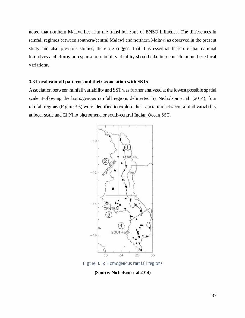
37

noted that northern Malawi lies near the transition zone of ENSO influence. The differences in

rainfall regimes between southern/central Malawi and northern Malawi as observed in the present

study and also previous studies, therefore suggest that it is essential therefore that national

initiatives and efforts in response to rainfall variability should take into consideration these local

variations.

3.3 Local rainfall patterns and their association with SSTs

Association between rainfall variability and SST was further analyzed at the lowest possible spatial

scale. Following the homogenous rainfall regions delineated by Nicholson et al. (2014), four

rainfall regions (Figure 3.6) were identified to explore the association between rainfall variability

at local scale and El Nino phenomena or south-central Indian Ocean SST.

Figure 3. 6: Homogenous rainfall regions

(Source: Nicholson et al 2014)

38

Computing the association between regional rainfall index and SSTs anomalies in all the four

rainfall regions reveal recognizable association particularly after 1980s. Regional rainfall indices

are negatively correlated to both the ENSO SST index and the Indian Ocean SST index.

Correlation tends to be high with Indian Ocean particularly for rainfall regions 1 and 2 (Table 3.1).

However, for rainfall regions 3 and 4 correlation is particularly high with Nino 3.4 (Table 3.1). In

the four regions the highest correlation is between rainfall region 1 and the Indian ocean SST with

correlation value of -0.745. The corresponding correlation value for association between rainfall

region 1 and the Nino 3.4 is -0.552. A similar pattern is seen in rainfall region 2 where

corresponding correlation values for association with the Indian ocean SST and with the Nino 3.4

are -0.509 and -0.276 respectively.

On the other hand, the correlation value for association between rainfall region 3 and the Nino 3.4

is -0.592 while the corresponding correlation value for association with Indian ocean SST is-0.363.

A comparable association is observed in rainfall region 4 where corresponding correlation values

for association with the Nino 3.4 are -0.430 and with Indian ocean SST is -0.148 respectively.

Comparison of the correlation coefficient values suggest that effects of the Indian Ocean SST in

the northern region of Malawi are stronger than those of ENSO SST. In southern and central

region, correlation of regional rainfall indices with the Nino 3.4 is found to be relatively higher

than that of the Indian Ocean SST, with the Indian Ocean SST having the weakest influence in the

central region.

Table 3.1: Correlation between regional rainfall index and SSTs anomalies

Indian Ocean SST Nino 3.4

Region 1 -0.745 -0.553

Region 2 -0.509 -0.276

Region 3 -0.363 -0.592

Region 4 -0.148 -0.430

Variability of rainfall in region 1, which has the highest correlation value of -0.745 between rainfall

and the Indian ocean SST was plotted to display the temporal pattern of rainfall in the region

(Figure 3.7). Figure 3.7 support the results of the previous studies (e.g. Funk et al 2008; Rocha

and Simmonds 1997) that anthropogenic warming of the SSTs in the south-central Indian Oceans,

is associated with decreasing rainfall over region 1. Figure 3.7 also supports the findings of

39

previous studies which suggested that the Indian Ocean contributes more to regional rainfall

variability in southern Africa (Goddard and Graham 1999; Goddard et al. 2001)

Figure 3. 7: Regional rainfall and SST series

3.4 Monthly variability of rainfall and its association with SST

Variability of rainfall and its association with SST anomalies was also analyzed at monthly time

scale. Analysis of rainfall at monthly time scale is more appropriate for or applicable to agricultural

livelihoods. For crops such as Maize, the staple for Malawi, the timing of rainfall fluctuations in a

season may have adverse implications on the crop. Shortage of moisture at some stages in the

growth of maize, particularly seed germination and milking stage may lead to failure of the crop.

Nkhata Bay is one of the wettest parts of the country with the longest rainy season. Unlike the rest

of the country where the rain season whereby the rain season is for 5 months from November –

April, in Nkhata Bay rainfall is concentrated in the months of November to May, with maximum

rainfall occurring in March. Correlation analysis show that the decreasing monthly rainfall series

are associated with the increasing south-central Indian Ocean SST series. Association is not evenly

distributed throughout the rainy season. The beginning in which December has the strongest

correlation and end of the rainy season are most sensitive to the southern eastern Indian Ocean

SST. However, the association is much more concentrated in the late months of the season i.e.

March, April and May. Corresponding correlation values for November – May are -0.387, -0.674,

-2

-1.5

-1

-0.5

0

0.5

1

1.5

1970 1975 1980 1985 1990 1995 2000 2005 2010 2015

No

rmal

ised

an

om

alie

s

Regional rainfall, Nino 3.4, & Indian Ocean SST series

Indian Ocean SST Rainfall Region 1 Nino 3.4

40

-0.390, -0.079, -0.459, -0.428, and -0.585 respectively. December has the strongest correlation the

associations. February have the weakest association. Since 1980s there is recognizable association

between increasing south-central Indian Ocean SST and decreasing rainfall in May in Nkhata Bay

(Figure 3.8).

Figure 3. 8: May rainfall and SST series

Although rains at the height/middle of the season seem virtually unaffected, sensitivity of

precipitation at the beginning and end of the rainy season to increasing SST of southern eastern

Indian Ocean have serious practical implication for smallholders. As Funk et al 2008 pointed out

the trend persist or intensify. Increased likelihood of failure or decreasing precipitation at the

beginning and end of the rainy season implies shortening of the growing season. Local farmers in

Nkhata Bay and Balaka in chapter 2 had observed that rainfall season is shortening. Farmers

observation were substantiated by meteorological records which showed a decreasing trend in the

number of days between 1st February and the end date of the rainy season for both locations, Balaka

and Nkhata Bay. Further analysis (Figure 3.9) show that the length of the growing/rainy season

(i.e. decreasing trend in the number of days between 1st February and the end date of the rainy

season) is negatively associated with increasing SST over the south-central Indian Ocean.

-2

-1.5

-1

-0.5

0

0.5

1

1.5

19

72

19

74

19

76

19

78

19

80

19

82

19

84

19

86

19

88

19

90

19

92

19

94

19

96

19

98

20

00

20

02

20

04

20

06

20

08

20

10

20

12

No

rmal

ise

d a

no

mal

ies

Monthly (May) rainfall variability and Indian Ocean SST series

Ind_Ocn SST May

41

Figure 3. 9: End of rainy season and SST series

With the specialized agriculture (i.e. maize monoculture) which is sensitive to moisture deficits,

the increased frequency of occurrence of weather perturbations is negatively affecting people’s

livelihoods. With the knowledge that the anthropogenic warming of the south-central Indian Ocean

will persist or intensify, there is fear that without effective adaptation, the rural livelihoods crisis

is likely to persist.

4.0 CONCLUSION

The study has shown that rainfall in Malawi is highly variable in time and space. Rainfall

variability in Malawi is associated with SSTs specifically El Nino Southern Oscillation (ENSO)

and south-central Indian Ocean SSTs. The study has also revealed that there is a tendency for

precipitation variability in the central and southern regions of the country to be negatively linked

Nino 3.4. Thus, anomalously warm SST in the tropical pacific are closely linked with occurrence

of dry conditions over a larger part of Malawi. However, the association between ENSO and

occurrence of dry conditions over Malawi is not uniform. Over the southern and central Malawi

occurrence of dry conditions is associated with El Nino condition. La Nina years are linked with

wet conditions. However, there is a relatively strong positive correlation between rainfall and El

Nino condition i.e. positive Nino 3.4 SST in the northern part of Malawi close to Tanzania. La

-1.5

-1

-0.5

0

0.5

1

1.5

1978 1980 1982 1984 1986 1988 1990 1992 1994 1996 1998 2000 2002 2004 2006 2008 2010 2012

No

rmal

ised

an

om

alie

sRaindays after 1st February, Nino 3.4, & Indian Ocean SST series

Ind_Ocn SST Nino Raindays

42

Nina years are linked with dry conditions. While some places show a strong correlation, and other

places show moderate to no association, or the reverse. The study has also established that at local

level in the north rainfall variability is strongly associated with south-central Indian Ocean SST

while in the south rainfall variability is strongly associated with El Nino phenomenon. Perhaps

most importantly, there are strong indications that variability is not distributed evenly throughout

the rainy season. Instead, rains at the middle of the rainy season are less associated with the SST,

whereas precipitation at the beginning, and particularly at the end, of the season are most prone to

failure or are more sensitive to SST anomalies.

43

Chapter 4: Climate Vulnerability Mapping: A Systematic Review and Future Prospects

Co-Authors: A. de Sherbinin, A. Bukvic, G. Rohat, M. Gall, B. McCusker, B. Preston, A.

Apotsos, C. Fish, S. Kienberger, P. Muhonda, O. Wilhelmi, D. Macharia, W. Shubert, R.

Sliuzas, B. Tomaszewski, S. Zhang

Abstract

Maps synthesizing climate, biophysical and socioeconomic data have become part of the standard

tool-kit for communicating the risks of climate change to society. Vulnerability maps are used to

direct attention to geographic areas where impacts on society are expected to be greatest and that

may therefore require adaptation interventions. Under the Green Climate Fund and other bilateral

climate adaptation funding mechanisms, donors are investing billions of dollars of adaptation

funds, often with guidance from modelling results, visualized and communicated through maps

and spatial decision support tools. This paper presents the results of a systematic review of 84

studies that map social vulnerability to climate impacts. These assessments are compiled by

interdisciplinary teams of researchers, span many regions, range in scale from local to global, and

vary in terms of frameworks, data, methods, and thematic foci. The goal is to identify common

approaches to mapping, evaluate their strengths and limitations, and offer recommendations and

future directions for the field. The systematic review finds some convergence around common

frameworks developed by the Intergovernmental Panel on Climate Change, frequent use of linear

index aggregation, and common approaches to the selection and use of climate and socioeconomic

data. Further, it identifies limitations such as a lack of future climate and socioeconomic

projections in many studies, insufficient characterization of uncertainty, challenges in map

validation, and insufficient engagement with policy audiences for those studies that purport to be

policy relevant. Finally, it provides recommendations for addressing the identified shortcomings.

44

Visual abstract

Maps of climate vulnerability have addressed a range of issues, such as (clockwise from upper

left) vulnerability to malaria, socioeconomic vulnerability to future climate risks, vulnerability to

floods, and vulnerability of elderly to storm surge, with a range of framings (center).

45

1. INTRODUCTION

With the advent of the Green Climate Fund and other bilateral climate adaptation funding

mechanisms, donors are directing billions of dollars of adaptation funds toward high need areas

based on climate vulnerability assessments, including climate vulnerability maps (Muccione et al.

2016, Klein 2009). The United Nations Environment Programme’s (UNEP) Research on Climate

Change Vulnerability, Impacts and Adaptation (PROVIA), a comprehensive effort to assess the

state of vulnerability assessment for adaptation planning, states explicitly that measuring and

mapping vulnerability is a top research priority (PROVIA 2013). Maps have been used to identify

areas of social vulnerability to climate hazards such as flood, drought, and sea level rise

(Notenbaert et al. 2010, Lam et al. 2015, Islam et al. 2013) and health impacts such as malaria

(Hagenlocher & Castro 2015), dengue (Dickin et al. 2013), extreme heat (Reid et al. 2009, Weber

et al. 2015) and food insecurity (Kok et al. 2010, Thornton et al. 2008, van Wesenbeeck et al.

2016) (Figure 4.1). End users have found the information contained in vulnerability maps useful

for planning adaptation assistance (de Sherbinin et al. 2017), understanding the underlying factors

contributing to vulnerability (Preston et al. 2009), emergency response and disaster planning

(Blaikie et al. 1994), risk communication and informing risk-reduction decision-making (Patt et

al. 2005, Edwards et al. 2007), and land use management (UNDP 2010). Given the research and

policy priority given to mapping vulnerability, it is imperative to develop a better understanding

of suitable approaches to vulnerability mapping across a range of scales, regions, climate hazards,

and thematic foci.

46

Figure 4. 1: Examples of vulnerability maps

Several literature reviews exist in allied areas. For example, Preston et al. (2011) reviewed the

state of climate vulnerability mapping up until 2010 based on a sample of 45 studies that, contrary

to this paper’s focus on social vulnerability, included the vulnerability of economic sectors and

ecosystems. de Sherbinin (2013) examined 15 global and nine regional hotspots mapping studies—

including some derived purely from climate model outputs and others using process-based models

to understand water or food system impacts—to identify common issues in underlying approaches

47

and regions at risk from the most severe climate impacts. Kienberger et al. (2013) evaluated 20

mapping studies in respect to their treatment of scale, time periods covered, vulnerability and

hazard focus, methods, and map products. Gall et al. (2015), based on a review of 1,006 journal

articles, evaluated the degree to which disaster risk research is truly integrated across scales,

stakeholders, knowledge domains, disciplines, and methods. Rufat et al. (2015) analyzed 67 flood

disaster case studies with regard to measurement approaches for social vulnerability to floods.

Rasanen et al. (2016) evaluated 125 climate vulnerability studies to identify interacting factors that

affect vulnerability. And finally, Jurgilevich et al. (2017) reviewed 42 sub-national climate risk

and vulnerability assessments to assess the degree to which changes over time (dynamics) were

incorporated. While all of these studies have made valuable contributions to our understanding of

vulnerability mapping and interdisciplinary research, there remains a need for a comprehensive

and systematic review of the state of the art in mapping social vulnerability to climate change.

To bridge this gap, we systematically assessed 84 vulnerability mapping studies with the goal of

encouraging further methodological refinement and identifying outstanding examples that could

help to guide future work in this area. This study has three objectives: 1) characterize current

practices in climate vulnerability mapping, 2) identify best practices and limitations, and 3) provide

recommendations that chart the way forward for future efforts. This paper is organized as follows.

The next section reviews the methods employed. This is followed by a characterization of the

studies, a review of the current state of practice, and assessment of policy relevance. The last

section points to future directions for research and practice followed by brief conclusions.

2. MATERIALS, METHODS AND DATA

The systematic review of vulnerability mapping case studies presented here draws on meta-

analytical and synthesis methods (Qin and Grigsby 2016, Magliocca et al. 2015, Berrang-Ford et

al. 2015). This included the development of study selection criteria, a standardized vulnerability

mapping evaluation protocol, and a thematic coding scheme.

We adopt a broad definition of vulnerability, which is the degree to which a system or population

is likely to experience harm due to exposure to perturbations or stress (Turner et al. 2003). For our

selection criteria, studies had to include both climate hazard (or exposure) and differential social

vulnerability. Climate hazard could be represented by past, present, or future climate variability,

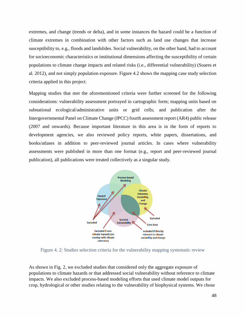
48

extremes, and change (trends or delta), and in some instances the hazard could be a function of

climate extremes in combination with other factors such as land use changes that increase

susceptibility to, e.g., floods and landslides. Social vulnerability, on the other hand, had to account

for socioeconomic characteristics or institutional dimensions affecting the susceptibility of certain

populations to climate change impacts and related risks (i.e., differential vulnerability) (Soares et

al. 2012), and not simply population exposure. Figure 4.2 shows the mapping case study selection

criteria applied in this project.

Mapping studies that met the aforementioned criteria were further screened for the following

considerations: vulnerability assessment portrayed in cartographic form; mapping units based on

subnational ecological/administrative units or grid cells; and publication after the

Intergovernmental Panel on Climate Change (IPCC) fourth assessment report (AR4) public release

(2007 and onwards). Because important literature in this area is in the form of reports to

development agencies, we also reviewed policy reports, white papers, dissertations, and

books/atlases in addition to peer-reviewed journal articles. In cases where vulnerability

assessments were published in more than one format (e.g., report and peer-reviewed journal

publication), all publications were treated collectively as a singular study.

Figure 4. 2: Studies selection criteria for the vulnerability mapping systematic review

As shown in Fig. 2, we excluded studies that considered only the aggregate exposure of

populations to climate hazards or that addressed social vulnerability without reference to climate

impacts. We also excluded process-based modeling efforts that used climate model outputs for

crop, hydrological or other studies relating to the vulnerability of biophysical systems. We chose

49

to limit our research to English language literature since it is the dominant language of

international science. To identify candidate studies, we conducted searches on Google Scholar

and the Web of Science using combinations of the keywords “vulnerability mapping”, “climate

change”, and “social vulnerability” (restricting searches to studies published after January 2007).

Table 1 shows that depending on the combination of terms used, the two search engines yielded

results ranging from 129 to more than 10,000 entries. Owing to our interest in including gray

literature such as reports produced by or for development agencies, we chose to use Google

Scholar, focusing on the union of the three search terms (Table 1, row 3). We sorted the Google

Scholar search results by relevance, and then evaluated the studies individually. Only studies that

fully met our criteria were retained. Our total sample included 84 studies covering a range of

geographic regions, thematic areas, and spatial scales (see Supplementary Online Materials

(SOM) for details on the search methods, and Table S1 for the full list). The final sample

comprised 62 journal articles, 18 reports, two white papers, one book chapter, and one

dissertation.

50

Table 4.1: Search results using online search engines: the Web of Science and Google Scholar (June 2016).

Search keywords Web of

Science

Google

Scholar

“vulnerability mapping” 10,087 >4,000

“vulnerability mapping”, “climate change” 639 2,100

“vulnerability mapping”, “climate change”, “social

vulnerability”

129 547

To develop the evaluation protocol, we collated available guidance regarding vulnerability

assessment and mapping as well as the mapping of information for communication and decision-

support (BMZ 2014, de Sherbinin 2014, Preston et al. 2011, Fussel 2007). The criteria included

aspects such as clear identification of the external hazard and valued attributes of the

socioeconomic system, a sound conceptual framework, evaluation of data layers, testing of

alternative integration and aggregation schemes, proper selection and use of climatic data,

sensitivity analysis, communication of study limitations and uncertainty, input data citation, and

adherence to basic cartographic conventions. The authors and four additional experts (see

acknowledgments) then qualitatively examined the selected vulnerability mapping studies to

benchmark the state of practice. Additional fields were included for thematic coding, such as

disciplines of authors, region, and spatial extent. The evaluation protocol and thematic coding

scheme were developed and implemented in Google Forms (see SOM Box S1 for the full list of

fields and response options). While only the 84 studies published during the decade from 2007 to

2016 formed the basis for our statistical characterization of the literature (Section 3), more recent

studies are used to illustrate good vulnerability mapping practice.

Initially, at least two coders reviewed each study. The evaluation criteria ranged from objective

‘facts’ to items that required some degree of subjective interpretation by the expert coders. In order

to harmonize the coding for these subjective items, the authors met at a workshop in May 2017

and individual coders resolved differences through a re-review of the case studies.

51

3 RESULTS

3.1 Characteristics of the Studies

Geographic coverage. Our sample covered a wide range of geographic regions (Fig. 4.3). Only

five studies were global in scope. Of the non-global studies, 35% were situated in Africa, 20%

each featured Asia and North America, followed by Europe (15%), Oceania (5%), and South

America (3.8%). In terms of country coverage, many studies are focused on the U.S. (10), followed

by Germany (5), Australia, India, and Nigeria (4 each).

Top journals. The top five publication outlets of the sampled climate vulnerability assessments

were Natural Hazards (8 studies), Climatic Change (6), Applied Geography (5), Global

Environmental Change (3), and Natural Hazards and Earth System Sciences (3). The studies

appear in a total of 38 different journals, with a strong representation of geography, health and

interdisciplinary journals focusing on climate change or natural hazards.

Level of analysis. The level of analysis varied widely, and a few studies used multiple levels. The

majority of studies in our sample were focused on local areas (e.g. watersheds or municipalities)

(26 studies). The remainder bounded their mapping at global (6), continental (5), regional (10),

national (19), and subnational (e.g., state or provincial) (18) levels (Table S1). Whatever the level,

all studies examined units within those bounding areas, either using natural/administrative units or

grids (see scale of analysis below).

Study goals. Authors cited a number of purposes for undertaking vulnerability mapping, and most

studies cited more than one. Hotspots identification was the primary purpose of many studies (57

total), followed by adaptation targeting (37), methodological refinement (34), disaster risk

reduction (34), spatial/development planning (21), strategic planning (12), baseline assessment

(11), advocacy (6), and monitoring and evaluation (2).

Valued attributes. The studies in our sample cited a variety of valued attributes (i.e., the system

or thing that may be harmed or lost owing to climate impacts) with most addressing more than

one. Health was pre-eminent among them (35 total; heat-stress and nutrition led the list), followed

by social impacts (33 total; poverty and demographic change were most often the focus), livelihood

impacts (31 total; especially agricultural livelihoods), economic impacts (20 total; especially

assets), and ecosystems as they relate to human wellbeing (5).

52

3.2 The State of Practice

Here we assess the studies in terms of interdisciplinarity, vulnerability framing, indicators and

aggregation approaches, data and projections, and treatment of uncertainty.

Interdisciplinarity. The field of vulnerability mapping is highly interdisciplinary; out of 80

studies with multi-authorship, 57 (71%) had authors from two or more fields of study. Geographers

were disproportionately represented in our sample, with 45% of lead authors from that discipline

(Figure 4.3), followed by earth and environmental science (14%), economics (10%), agronomy

and engineering (6% each), and a smattering of other disciplines. The disciplinary background of

the authors appears to influence the degree to which the climatic exposure versus social

vulnerability aspects were emphasized in the study. In some studies, the social vulnerability

aspects were developed in great detail, but climate exposure metrics were weak (e.g., Kienberger

et al. 2012, Udoh 2015, Lawal and Arokoyu 2015). In other studies, the opposite was the case

(e.g., Kim et al. 2015, Piontek et al. 2013).

Figure 4. 3: Studies by Continent, Level of Analysis, and Discipline

Vulnerability framing. Close to 60% of the studies draw on the framings of vulnerability and risk

developed by the IPCC Working Group II across several assessment reports. The IPCC Third

Assessment Report (TAR) and AR4 vulnerability frameworks (McCarthy et al. 2001 and Parry et

al. 2007, respectively) identify vulnerability as a function of exposure to climate hazards, on the

one hand, and the sensitivity and adaptive capacity of the system or society on the other. In 2012,

the IPCC Special Report on Extremes (IPCC 2012) introduced a risk framework, also adopted by

the Fifth Assessment Report (AR5) (Oppenheimer et al. 2014), which distinguished between

53

exposure and vulnerability, the latter combining the sensitivity and adaptive capacity elements of

the earlier frameworks. The “vulnerability” element in this risk framing thus represents social

vulnerability or other types of vulnerability (e.g., ecosystems or infrastructure), depending on the

study. Some argue that this more clearly separates out the climatological/hazard elements from the

system being exposed (Cardona et al. 2012). While both risk and vulnerability framings may

include social vulnerability, risk management tends to focus on the probability distributions of

extreme weather events and long term trends of certain magnitudes, which is vital for disaster

preparedness and infrastructure construction, whereas vulnerability assessments tend to emphasize

underlying factors that put people and infrastructure at risk (de Sherbinin 2014).

Of the studies in our sample, one-third used the IPCC AR4 vulnerability framework (Parry et al.

2007), 17% utilized the very similar IPCC Third Assessment Report (TAR) vulnerability

framework (McCarthy et al. 2001), and 10% utilized different risk frameworks, including the AR5

risk framework. The only studies in our sample that explicitly adapted the SREX framework were

Kienberger and Hagenlocher (2014), Hagenlocher and Castro (2015), and de Sherbinin et al.

(2014a). A number of studies mapped risk more broadly (Carrao et al. 2016, Aubrecht & Özceylan

2013, Poompavai and Ramalingam 2013, Scheuer et al. 2011, Johnson et al 2009). Another 3.5%

used livelihood frameworks (Carney et al. 1998), and 36.5% used a variety of custom or derivative

framings. For example, some studies (e.g., Behanzin et al. 2016, Papathoma-Koehle et al. 2007)

developed their own vulnerability framing, or adapted frameworks developed by others (e.g.,

Wang & Yarnal 2012, Fekete 2009).

Whatever the choice of framework, it needs to be “fit for purpose” in terms of illuminating the

features of interest in the complex coupled human-environment system. At a minimum, any

quantitative vulnerability assessment requires definition of the system of analysis (what is

vulnerable?), the valued attributes of concern (why are they important?) (Figure 4.4), the external

hazard (to what is the system vulnerable?), and a temporal reference (when?) (Füssel 2007).

Preston et al. (2009) also note that when vulnerability mappers engage with stakeholders, including

decision-makers, the framing must take into account their needs and desired outcomes.

Participation of end users can ensure that the choice of framework and subsequent assessment

process meets users’ needs and increases the usability of map products.

54

Figure 4. 4: Summary of the studies in terms of (a) method of spatial analysis, (b) valued

attribute, and (c) aggregation method

Non-Climate Indicators. In general, authors relied upon census or survey data for socioeconomic

indicators as proxies for sensitivity and adaptive capacity (Hinkel 2011), and only rarely collected

data (e.g., Kienberger 2012). Common proxies for social vulnerability included age, race, income,

and education, which are readily available parameters. Rarely were outcome measures such as

malnutrition, body mass index, or morbidity employed (e.g., van Wesenbeeck et al 2016, de

Sherbinin et al. 2014b). Furthermore, papers varied in their consideration of past literature to

identify relevant drivers of vulnerability; for example, Tapia et al. (2017) conducted an exhaustive

literature review of 150 studies to identify climate impact chains in Europe cities and to select

indicators of vulnerability across multiple exposure types. Non-climate biophysical indicators

included land use and land cover (50% of studies), geographic proximity to physical features (e.g.,

coasts, rivers, roads) (38%), or vegetation types (26%), soil (19%), and topography (12%) (Fig.

5). With the exception of Rasanen et al. (2016), no studies considered exposure to non-climatic

stressors, such as economic downturn or health crises, in addition to climatic stressors.

Fekete (2012) notes common problems of socioeconomic data include measurement errors, biased

samples, geographic gaps, missing values, infrequency of updates, data decay and inappropriate

normalization. To obtain more frequently updated socioeconomic parameters, there are growing

efforts to use remotely-sensed proxies for poverty, such as housing structure in slums (Ebert et al.

55

2009) or “nightlights poverty” (Davies et al. 2010), as well as for other parameters (de Sherbinin

et al. 2015). None of the studies in our sample used other non-traditional data sources such as cell-

phone call detail records and recharge rates or geo-located social media, though these data sources

are showing increasing promise for mapping daily mobility patterns related to hazard exposure as

well as vulnerability (Yu et al. 2018).

Climate-related parameters and projections. The climatic variables and climate-related

processes and phenomena of greatest interest included temperature and precipitation (48% of

studies each), flood (44%), drought (21%), sea level rise (13%), cyclones (12%), storm surge

(10%), heatwaves (7%), coastal or riparian erosion (6%), bushfires (6%), and landslides (6%)

(Figure 4.5). Among 31 papers that incorporated climate data, 35% incorporated long-term

climatic averages, followed by daily data (32%), monthly and annual data (13% each), and

seasonal parameters (6%).

Most vulnerability mapping studies focused on the present-day climate or recent past (Jurgilevich

et al. 2017). Thirty-one studies (36%) included future projections, and of these 70% used climate

projections but no socio-economic projections; 17% included both climate and socio-economic

projections; 6.5% employed socioeconomic projections only; and 6.5% used scenarios of sea level

rise. For those that did utilize future climate projections, 38% had ensemble scenarios (multi-

model, multi-scenario) based on the mean values (e.g. Filho et al. 2016, Torres et al. 2012, Thorton

et al. 2008), whereas the remainder used one model, a practice generally discouraged by the climate

science community (Knutti et al. 2010). For example, the European Spatial Planning Observation

Network (ESPON) Climate report used only one model and one scenario: the COSMO Climate

Limited-area Modelling (CCLM) and the special report on emissions scenarios (SRES) A1B

(ESPON 2013). Several other studies also used only the SRES A1B scenario (Holsten and Kropp

2010, Lissner et al. 2012, Busby et al. 2014, Corobov et al. 2013). The use of single models with

one scenario makes it difficult to characterize uncertainty (see below). In our sample, only Liu et

al. (2008), Müller et al. (2014), and de Sherbinin et al. (2014b) used multiple scenarios with

confidence intervals bounding the results. A more recent study (Mani et al. 2018) used 11 GCMs,

selected on their ability to reproduce past climate, to project climate changes over South Asia, and

a few other studies in our sample (e.g., Busby et al. 2014, Torres et al. 2012, Preston et al. 2008)

approach best practices by employing state-of-the-art modeling of future climate.

56

Figure 4. 5: Summary of the studies, clockwise from upper left, in terms of (a) timeframes of

analysis (%), (b) temporal nature of the climate parameters considered (%), (c) spatial data layers

or parameters considered (no.), and (d) climate-related phenome

In terms of downscaling, 11% of the studies used coarse spatial resolution (0.5 to 1 degree) global

climate models (GCMs), 7% used downscaling -- dynamical (1) or statistical (5) -- and 6% used

regional climate models (RCMs) at moderate to fine spatial resolution. The appropriateness of

GCMs for local-level assessments is a matter of debate; for broader continental-scale studies these

may be sufficient, but for any smaller regions or areas with significant topography, it is generally

desirable to use downscaled climate projections or RCMs (Trzaska and Schnarr 2014). While

GCMs may not adequately represent local climatic conditions, the uncertainty introduced by

different downscaling methods need to be taken into consideration (Barsugli et al. 2013).

Aggregation methods. The sample of case studies presented a variety of methods for data analysis

and aggregation, with index construction being the most common. Sixty-one percent of the studies

produced a vulnerability index with sub-components (i.e., hierarchical models), whereas 14%

developed indices without components, 11% produced components but no overall index, and 5%

57

featured separate indicators (or variables) without indices. An index was calculated for 2% of

studies but without presentation of the components. Only 7% had no index or indicator

construction (Figure 4. 4), being based on overlay, cluster or regression analysis.

Fifty percent of studies relied on linear aggregation for index construction, 62% of which used

weighting based on expert input or judgment of the researchers on the relative importance of

indicators. Data reduction strategies appeared in 21% of studies, generally using principal

components analysis (PCA) and subsequent linear aggregation. Other, less common, aggregation

schemes included cluster analysis (3.5%), spatial regression modeling (7%), geometric mean (7%),

and geon or spatial segmentation (5%). Five studies had insufficient methods description to

determine the approach used, a major shortcoming. In some cases (e.g. Baum et al. 2009), PCA

was used for the construction of a social vulnerability index, after which linear aggregation was

used with the remaining indicators.

The statistics of index construction and the many alternative ways of constructing indices is the

subject of a growing literature (Greco et al. 2018, Reckien 2018, Becker et al. 2017, Tate 2012,

Rufat et al. 2015, Nardo et al. 2005), and issues at each stage of construction—the choice of

indicators, analysis scale, measurement errors, transformation, normalization, factor retention (in

PCA), and weighting—all influence results (Tate 2012). Much of the work in our case studies

sample simply adapted methods or approaches from prior vulnerability mapping work, resulting

in derivative approaches applied to new regions. Statistical best practices, such as uncertainty

analysis/sensitivity analysis or validation (below), are underutilized. Exceptions included Mainali

& Pricope (2017) and de Sherbinin et al. (2014b), both of which compared results from linear

aggregation and PCA and conducted sensitivity analyses. Lastly, many of the studies displayed

scant awareness of the statistical implications of their index construction methods (e.g., issues of

compensability or co-linearity in linear aggregation), a general failing across many studies of

social vulnerability (Tate 2012).

Scale of Analysis. The choice of bounding box (level of analysis) and spatial unit of analysis are

important, and have ramifications for the approach to data integration (given multiple formats and

scales of data inputs) and the statistical properties of the inputs and outputs. A more complete

review of scale issues in data integration are found in Fekete et al. (2010), Kienberger et al. (2013),

58

and de Sherbinin (2014 and 2016). Fifty-five percent of our studies used administrative units,

followed by grid cells (40%), and geons (2%). One study each used natural units or parcel/property.

Ideally, the choice of spatial unit would be determined by the scale of action (Cao and Lam 1997),

that is, the scale at which variation in vulnerability is best observed or at which decisions need to

be made. All too often the choice of common scale for data integration is pragmatically dictated

by the measurement scale of available and accessible data – which could be the coarsest or finest

resolution data set – rather than the operational scale. While coarser resolution data sets can be

resampled, that does not change the underlying or nominal scale. For example, climate projections

may have grid cell sizes of 0.5 to 1 degree, and may be resampled at higher resolution to integrate

with higher resolution data, but the result is blocks of rasters with the same values. Few studies

addressed the implications of their level or unit of analysis on their results; one that did, Abson et

al. (2012), found that results depended heavily on how the bounding box was drawn.

Treatment of uncertainty. It is widely accepted that uncertainty levels are high in studies of

climate vulnerability, especially at the science-policy interface (Kunreuther et al. 2014). This is

partly a function of the diverse data streams from social and natural sciences that are used to

construct vulnerability maps, and the uncertainties that are contained in each type, and partly due

to the emergent nature of vulnerability arising out of complex coupled systems (Holling 2001,

Soares et al. 2012) which forces developers to use indicators as proxies (indirect measures) of the

phenomenon of interest such as e.g., likely or potential harm from impacts (Hinkel 2011).

Uncertainties are compounded when projections are used. Uncertainty results from lack of

precision or accuracy in the measurement of the climatic, natural or socioeconomic variables that

contribute to vulnerability, which in turn may be due to a host of factors such as poor

instrumentation, systematic biases (sampling or model biases), and spatial interpolation of data

between measurement points, all of which contribute to both systematic and random error. Table

4.2 characterizes different types of spatial, temporal and attribute uncertainties that may be present

in different types of geospatial data.

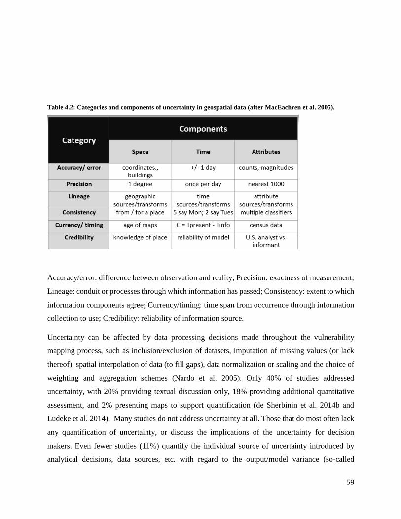
59

Table 4.2: Categories and components of uncertainty in geospatial data (after MacEachren et al. 2005).

Accuracy/error: difference between observation and reality; Precision: exactness of measurement;

Lineage: conduit or processes through which information has passed; Consistency: extent to which

information components agree; Currency/timing: time span from occurrence through information

collection to use; Credibility: reliability of information source.

Uncertainty can be affected by data processing decisions made throughout the vulnerability

mapping process, such as inclusion/exclusion of datasets, imputation of missing values (or lack

thereof), spatial interpolation of data (to fill gaps), data normalization or scaling and the choice of

weighting and aggregation schemes (Nardo et al. 2005). Only 40% of studies addressed

uncertainty, with 20% providing textual discussion only, 18% providing additional quantitative

assessment, and 2% presenting maps to support quantification (de Sherbinin et al. 2014b and

Ludeke et al. 2014). Many studies do not address uncertainty at all. Those that do most often lack

any quantification of uncertainty, or discuss the implications of the uncertainty for decision

makers. Even fewer studies (11%) quantify the individual source of uncertainty introduced by

analytical decisions, data sources, etc. with regard to the output/model variance (so-called

60

sensitivity analysis) (Saisana et al. 2005). The paucity in uncertainty and/or sensitivity analysis is

most prevalent with regard to socioeconomic models or the combination of biophysical and

socioeconomic data.

Uncertainty estimates are especially important when variables at differing scales are collected and

overlaid for interpretation. The issue of error induced with the introduction of each variable can

quickly render an analysis little more than “guesswork” if error is not mapped or in some other

way accounted for, yet only 18% of studies discussed here provided any quantitative assessment

of error and only 2% mapped error. Even when systematic measurement of uncertainty is not

possible, authors would do well to acknowledge data issues that contribute to uncertainty,

including spatial variation in uncertainty, owing to factors such as the density of measurement

points (or input unit size), sampling errors in demographic data, and data quality issues across

jurisdictions (de Sherbinin and Bardy 2016). Preston et al. (2011) summarized the issue well when

they stated that the failure to address uncertainty “often results in questions regarding the validity,

accuracy and precision of vulnerability maps, or, in other words, whether maps themselves

represent sufficiently robust visions of vulnerability to guide stakeholders regarding the potential

for harm.”

Data citation. Vulnerability mapping is data-intensive. Disclosure of all data inputs, data

processing, as well as assessment of data deficiencies, is important for the validity of results,

understanding uncertainties and replication by others (Parsons et al. 2010). Fifty-five percent of

studies provided only partial information on data inputs (e.g., through acronyms in a table of data

inputs), and 8% omitted references entirely. All other studies followed best practice by providing

full citations with URLs wherever possible or, better yet, full metadata on layers used.

The Map. Given the centrality of “the map” in vulnerability mapping, there is much room for

improvement in map design and adherence to cartographic conventions. In the reviewed studies,

maps are often too small, or suffer from common cartographic pitfalls such as poor color schemes

and inadequate attention to color-blind readers (Brewer 1994), overcrowding, and lack of spatial

reference information (major rivers, roads or settlements). Some of the cartographic limitations

may stem from restrictions on figure sizes imposed by journals. Still, given the amount of analysis

required to get to the point of producing maps, lack of attention to barriers that arise from poor

61

cartography and risk communication means that many studies that desire to influence policy may

fall short of their goal.

3.3 Policy Relevance

Most studies claimed to be policy relevant and emphasized the importance of vulnerability

mapping to adaptation planning, but very few studies provided specific policy recommendations

or engaged with policy makers and other stakeholders to frame the primary research questions or

to assess outcomes. Such engagement requires working relationships and demands additional

forms of inquiry such as interviews with stakeholders or follow-up research investigating the utility

of the maps. Given the claims of policy relevance by many studies, it is worthwhile exploring the

uptake of study results to gauge the transfer of research to practice as well as the efficacy of climate

vulnerability maps.

While many studies were academic in nature, and thus not geared toward policy makers, those that

claimed policy relevance often fell short of best practice. For example, several studies lacked

specificity regarding the valued attribute or the climate hazard of focus (e.g., Acosta et al. 2013,

Chakraborty and Joshi 2013, Hutton et al. 2011). Depending on the decision-maker and the

intended usage, vaguely defined maps of “vulnerable populations” are unlikely to lead to concrete

policy or implementation responses. Similarly, researchers often chose a multi-hazard approach to

social vulnerability index development (e.g., Busby et al. 2014, Chakraborty and Joshi 2013, Yusuf

and Francisco 2009). When it comes to implementation decisions, multi-hazard approaches with

overly broad definitions of social vulnerability provide limited guidance compared to more hazard-

specific vulnerability maps (e.g., vulnerability to flood, drought, heat stress, or cyclones), though

they can be effective for resource prioritization or risk communication to broader audiences.

Similarly, the chosen spatial scale of maps should match that of the decisions for which they are

likely relevant or useful. For example, in addition to providing gridded maps showing spatial

variation in vulnerability, policy makers may be interested in results aggregated to and/or ranked

by administrative units (e.g. rank position of average index scores), but this is rarely done

(exceptions include de Sherbinin et al. 2017). In addition, many studies – particularly those

covering large spatial extents – did not contextualize the results by elaborating on climate impacts

on sectors, systems or groups. While such maps can be useful for general risk communication,

their utility for decision making is limited. Without context or stakeholder engagement, maps may

62

become an end in themselves, rather than an entry point for discussion or “boundary object” for

discussion among stakeholders (de Sherbinin et al. 2017, Preston et al. 2011).

Only a few studies directly worked with decision makers (e.g. McCusker et al. 2016, Roy and

Blasche 2015, Weber et al. 2015, de Sherbinin et al. 2014b, Collins et al. 2013, Kienberger 2012,

Lindley et al. 2011, Preston et al. 2009). These studies generally found that the co-production of

knowledge was important to the success of the project. The majority of studies were academic

exercises driven by intellectual curiosity or methodological development. While this may be a

function of research objectives or funding source requirements, lack of engagement with

stakeholders may also stem from the fact that the co-production of knowledge takes time and a

commitment to process (Meadow et al. 2015). This includes listening to concerns, joint problem

identification and design of the analytical framework, choice of weighting schemes, interpretation

of the map products, communication of uncertainty, and design of adaptation interventions. Praxis

related activities often require a different skill set than the geospatial data integration and statistical

skills possessed by most vulnerability mappers, but they can be learned (Stuart and Hovland 2004).

4. RECOMMENDATIONS AND FUTURE DIRECTIONS

During the workshop, expert participants were asked to present and defend their choice of their

top two mapping studies, and time was set aside to discuss lessons from the identified studies that

could inform mapping practice. The following is a distillation of recommendations and future

directions for vulnerability mapping.

Improved cartography and decision support tools. As mentioned above, mapping conventions

were not uniformly followed in the studies. Vulnerability mappers would do well to interact with

decision makers to ensure that their map results can be easily understood by non-technical

audiences (Ishikawa et al. 2005, de Sherbinin et al. 2017), as well as data scientists, visualization

experts and cognitive scientists to evaluate different ways of mapping and visualizing vulnerability

information (Padilla et al. 2017, Dasgupta et al. 2015). At a minimum, the field would benefit from

the use of sequential color schemes in which a limited number of hues are used and the range is

illustrated with a change in saturation. Only in cases where there is a clear mid-point in the data

(e.g., z-scores or values that run both positive and negative) is it appropriate to use diverging color

schemes with two hues (Brewer 1994). Similarly if the data are categorical, using more than one

63

color is appropriate. In addition, well designed diagrams such as those included in Kienberger et

al. (2016) (Figure 4.6) or Kienberger and Hagenlocher (2014) are particularly helpful in

communicating the relationships among the elements of the framework.

Figure 4. 6: Diagram from Kienberger et al. 2016 illustrating the elements contributing to an

agricultural vulnerability index, including weighting of the variables and components

Maps should communicate uncertainty in the data and analysis. Retchless and Brewer (2016)

suggest that including uncertainty information on the map is more effective than including it in an

adjacent map, and that this inclusion does not interfere with map reading if done correctly. There

are a number of common methods for cartographic communication of uncertainty: One is to cross

hatch areas or increase the color saturation in areas where results are more certain, such as where

multiple climate model scenarios agree (Kaye et al. 2012). Another is to create fuzzy boundaries

(Kienberger 2012) or to run a low-pass filter (spatial averaging) over results. By interacting with

the end users, map developers can identify the best way to portray uncertainty.

As maps become more interactive and web-based, practitioners may find advantages in decision

support tools (DSTs). DSTs move beyond the presentation and representation of findings to help

formulate or test hypotheses, identify unknowns, and support decisions under a variety of

64

scenarios. Indeed geovisual analytics, as a field within GIScience, has identified the benefits of

interactive decision support maps (Andrienko et al. 2007), however there is a need for more

research in this domain that is focused on climate vulnerability mapping.

Beyond the map. Advanced data sources and statistical methods are moving beyond the mapping

of hotspots to help elicit the drivers of vulnerability and, by extension, what interventions are

possible (e.g., McCusker et al. 2016, van Weesenbeek et al. 2016). These approaches often use

relatively recent survey data (e.g., Demographic and Health Surveys or Living Standards

Measurement Surveys), tied to specific locations through the centroids of sample locations and

interpolated using spatial kriging, to tease out the factors contributing to vulnerability, along with

advanced statistics and geospatial analysis to target development interventions (e.g., Runfola et al.

2015).

As an example, livelihood-informed vulnerability analysis involves data analysis of large

household surveys on shocks and shock responses to determine factors that correlate with

resilience and vulnerability. McCusker et al. (2016) use three models -- logistic regression, spatial

eigenvector filter logistic regression, and geographically weighted regression -- to tease out the

drivers behind self-reported household shocks. Self-reported shocks were regressed with

demographics and the socioeconomic characteristics of the households across the country, and

results were mapped if significant in all the three models. This form of vulnerability mapping has

the advantage of creating detailed maps, statistics and graphics of the distribution of selected

variables and regression results over space.

Single index aggregation reduces the richness of information provided by the suites of individual

vulnerability indicators on which the maps are based, and can produce similar scores in two

locations where vulnerability is driven by very different processes. To gain a more holistic insight

requires an understanding of how multiple factors that exacerbate or mitigate vulnerability to

exogenous livelihood shocks vary in relation to each other (Abson et al. 2012). With additional

understanding of the local context, researchers are able to understand the shocks (e.g., weather,

food prices, financial, or health) that are most important to households, and determine appropriate

responses (McCusker et al. 2016). This underscores an important point: a map can serve to point

out differential vulnerability in a given area, but deeper field research is almost always required to

develop appropriate adaptation responses.

65

Mapping the future. Combining socioeconomic and climate scenarios will be increasingly

important for understanding the relative contributions of both changes in human factors

(demography, economic development, urbanization) and climatic factors in generating future

impacts. A key element for future work will be the inclusion of socioeconomic scenarios such as

those developed using the Shared Socioeconomic Pathways (SSPs) or similar approaches (O’Neill

et al. 2014).

While decades of climate research have led to a improved understanding of changes in the climate

system, albeit with limitations regarding climate sensitivity and extremes, very little has been

achieved so far to comprehend the future dynamics of human systems and its influence on future

vulnerability (Lutz and Muttarak 2017). Although projecting spatial socioeconomic characteristics

of populations into the future is difficult (O’Neill and Gettleman 2018), a number of methods have

already been developed (Rohat 2018) and the use of scenarios enables accounting for uncertainties

in future socioeconomic development trends. Strader et al. (2017) provide a rare example of

vulnerability mapping incorporating future scenarios. As such, the SSPs (O’Neill et al. 2014) offer

an unprecedented opportunity to integrate socioeconomic projections—and their uncertainties

under varying level of socioeconomic development—within assessments of future climate change

vulnerability (Wilbanks and Ebi 2014). The world is far more dynamic than most vulnerability

mapping efforts portray. Mapping efforts need to consider incorporating stochastic elements, such

as extreme climate events, conflict, or other shocks to the system. Mapping will also need to

acknowledge the dynamic connections between indicators, as well as linkages across scales

(Jurgilevich et al. 2017).

Validation. Many authors have noted the importance of validating vulnerability maps and the lack

of attention that such validation has received in studies to date (Preston et al. 2011, Hinkel 2011,

Tate 2012, de Sherbinin 2013, Tellman et al. 2017). This is attributable to a number of factors:

First, theoretical constructs of vulnerability are proxies for complex socio-ecological processes

that are difficult to measure and, therefore, validate (Vincent 2004). Second, vulnerability maps

often represent vulnerability in a generic sense – in the absence of the specific articulation of who

or what is vulnerable and to what, it is not clear what the associated outcomes should be. Third,

vulnerability maps attempt to represent an inherently uncertain future, for which there is no

observable information or data to validate maps against.

66

Given these challenges, a key question in vulnerability mapping is to what extent is validation

necessary? This is largely a function of the objective of the mapping exercise and how the map(s)

will subsequently be used. For maps generated as part of a research activity that is disconnected

from adaptation practice or decision-making, there may be little incentive to pursue validation.

Developing new methods or metrics for vulnerability analysis, for example, may not have a

practical application that merits validation. Vulnerability maps can be used to open a dialogue

around vulnerability, its meaning, and its causes (Preston et al. 2009). So, if the objective is to help

stakeholders conceptualize rather than predict vulnerability, validation may be unnecessary.

Often, vulnerability maps are intended as tools to support decision-making regarding the

prioritization and targeting of adaptation interventions and/or investments (Preston et al. 2011, de

Sherbinin 2014). This creates potential incentives for stakeholders to manipulate the assessment

of vulnerability in order to justify a priori policy objectives. In such situations, demonstrating that

indices are robust to both data inputs and outcomes of interest, including the characterization of

their uncertainties and limitations, is important (Saisana et al. 2005, Hinkel 2011, Tate 2012,

Weeks et al. 2013). Vulnerability metrics that do not accurately reflect the underlying outcomes

or processes of interest or that generate insights not reflected in other metrics significantly increase

the risk of type I and II errors (false positives and false negatives, respectively) that could waste

resources or prove maladaptive.

Specific methods for validation generally follow one of two approaches (Esnard et al. 2011, Tate

2012). The most common is external validation, where vulnerability metrics are validated against

independent outcomes of interest such as past health outcomes or economic losses from extreme

weather events (Patt et al. 2005, Preston et al. 2009, Preston et al. 2011, Tate 2012, Tellman et al.

2017). However, metrics that are validated against one type of outcome may not work for others.

For example, a metric capable of predicting historical disaster losses may not perform well in

predicting future health impacts or population displacement. There may also be biases in the

economic loss data used to validate the metrics, and there are issues with the fact that while a

hazard may impact all areas (e.g., floods or drought), the intensity of that hazard is likely to vary

spatially such that there is not equal treatment across all units in order to understand the dose-

response function. Finally, in many parts of the developing world, the data necessary for external

67

validation simply does not exist, nor is it likely to in the near future. Applications of external

validation must be cognizant of these limitations.

Alternatively, some researchers have opted to use internal validation—statistical tests and

sensitivity analysis—to assess the effects of metric construction on results (Tate 2012, Carrão et

al. 2016, Heß 2017). Neither approach, however, overcomes the challenge of validating estimates

of future vulnerability. This constraint should be acknowledged in the use of vulnerability metrics

and consideration must be given to the relevance of vulnerability metrics to understanding the

future implications of climate change.

Notwithstanding the difficulties of validation, it is important to continue to test methods of

validation, and for policy-oriented vulnerability mapping efforts to seek to validate indices

wherever possible, or the enterprise risks being discredited owing to claims that vulnerability maps

are unable to predict future harm.

Value of information. There are a number of ways to assess the likely uptake or impact of

vulnerability mapping for decision making, and we recommend that the community of researchers

involved in vulnerability mapping more rigorously test and evaluate the value of the information

provided. One approach, mentioned above, is to work directly with decision makers, data

visualization experts, and cognitive scientists to understand how decision makers read maps and

assimilate information. A number of promising future research directions include (a) semi-

structured individual or focus group interviews; (b) work observation; (c) think aloud protocols

(whereby subjects will verbally express what they are thinking about as they explore maps); (d)

online focus group or Delphi exercises (MacEachren et al. 2006); and (e) task analysis (de

Sherbinin et al. 2017). The aim would be to gauge policy-maker comprehension of the information

presented in maps, their preferences in map design (Retchless and Brewer 2015), their comfort

level with the uncertainty in map products, and, ultimately, how and why the information presented

in maps influenced their decisions.

In the field of economics, value of information research is demonstrating the societal benefit of

information for decision making by examining the economic costs associated with decision

making that was made prior to the introduction of new information, and measuring the economic

benefits (net of the cost of the new information sources) of improved decisions. Economic costs

could be measured in terms of lives lost, hospital visits, or economic damages. Recent work on

68

the value of satellite remote sensing information (Bernknopf and Brookshire 2018, Cooke et al.

2014) provide examples of rigorous economic analyses that could be performed for vulnerability

mapping.

5 CONCLUSION

Vulnerability mapping is growing field, and one that is likely to increase in importance given the

magnitude of expected temperature increases and associated impacts (World Bank and PIK 2012).

Such mapping acknowledges that the effects of climate change on society are not solely a function

of exposure to temperature and precipitation changes or increases in the frequency or magnitude

of extreme events, but that the sensitivity and adaptive capacity of societies to these changes will

play a crucial role in influencing outcomes. Mapping also acknowledges that all the factors that

contribute to vulnerability—e.g., exposure to extremes, land use and land cover, population

density, relative wealth and poverty, and institutional effectiveness—vary spatially, and that there

relative contributions to overall vulnerability are different from place to place (e.g., Nayak et al.

2017, Kienberger and Hagenlocher 2014). Thus, mapping can make significant contributions to

enabling society to effectively adapt, or to signal where adaptation may face sufficiently high

barriers that communities may be forced to migrate (Rigaud et al. 2018).

We find that vulnerability mapping as a field is maturing, but a number of issues remain that need

to be addressed for the field to advance, including increasing the degree of collaboration with end

users, greater attention to map communication, moving beyond the map as the final product, work

on validation, and greater justification for mapping based on value of information research. This

is all the more important as decision makers look to invest large sums of money in adaptation

assistance, and to justify their choices based on scientific tools such as vulnerability maps.

69

Chapter 5: Conclusion

This dissertation attempted to better understand deepening rural livelihood vulnerability in

Malawi. The study took a multidimensional approach to better analyze rural livelihoods

vulnerability in Malawi to leverage effective adaptation to climate change. Drawing on actual lived

experiences and local knowledge/perceptions of the changing climatic conditions and reviewing

the state-of-the-art literature on vulnerability analysis, the study has shown that rural livelihood

vulnerability can better be discerned using multidimensional approaches – combining natural and

social vulnerabilities. The dissertation has summarized the findings through 3 closely related

articles which have stretched/extended the ways to understand worsening rural livelihood

vulnerability. Local knowledge has shown that smallholders in Malawi are sensitive and

knowledgeable of the changing climatic conditions/environmental context that mediate their rural

livelihoods. Local farmers have observed changes with regard to onset, amount, length of season,

intensity and distribution of rainfall. Their observations are consistent with meteorological records.

Farmers perceptions reflect local vulnerabilities and concerns, i.e. actual impact of climate on

livelihoods. Such detailed knowledge about changes in rainfall pattern can be harnessed to

facilitate effective adaptation. Since research has shown local farmers react to change that they

observe, adaptation efforts/initiatives that can be tailored to local farmers perceptions can

enhance/ensure local agreement and participation to reduce the deepening rural livelihood

vulnerabilities.

Through correlational analysis the dissertation has shown that the changing environmental context

i.e. rainfall variability and dry conditions over Malawi are linked to teleconnections - SST over

Indian Ocean and El Nino conditions. The study further established that the association is not

uniform across, it varies spatially. Interventions therefore need to consider spatial variability. In

addition, the dissertation has also revealed that rainfall variability is not distributed evenly

throughout the rainy season. The beginning and end of the rain season are most prone to

failure/more sensitive to SST anomalies implying shortening of the growing season. As rural

livelihoods in Malawi are heavily dependent on rainfall and with maize as the staple crop which

is sensitive to moisture deficits increased rainfall variability and shortening of the rain season

pushes rural livelihoods further to the edge. This does not portend well for rural livelihoods with

the understanding that anthropogenic warming of the Indian Ocean will persist.

70

Through review of current practices in vulnerability analysis and mapping the dissertation has

highlighted that effects of climate change on society are not solely a function of exposure to climate

hazard, but that the sensitivity and adaptive capacity of societies to climate shocks will play a

crucial role in influencing outcomes. The dissertation has also pointed out that all the factors that

contribute to vulnerability vary spatially, and that their relative contributions to overall

vulnerability are different from place to place. Thus, mapping can make significant contributions

to enabling society to effectively adapt. The dissertation however has found that a number of issues

remain that need to be addressed for vulnerability mapping to be more effective and fruitful,

including increasing the degree of collaboration with end users, greater attention to map

communication, moving beyond the map as the final product, work on validation, and greater

justification for mapping based on value of information research. As maps have become part of

the standard tool-kit for communicating the risks of climate change to society and decision makers

depend more on maps to justify their choices of where to invest large sums of money in adaptation

assistance, it is more important that better and suitable approached to vulnerability mapping are

used and consequently good vulnerability maps are developed.

The research was not without challenges. One challenge was language. While I am fluent in the

languages that are widely spoken in Malawi (including study areas) some people in study areas

prefer to speak language that I am not familiar with. Another challenge was the terrain of the study

areas particularly in the north, Nkhata Bay. Nkhata Bay is mountainous and dwelling places are

distances apart with no means of transport. It was practically impossible to access the communities

in the rain season. This demanded a substantial amount of time to gather data. We had to put in

place a good and realistic work plan to minimize loss of time inefficiencies and make good use of

the available opportunities. We sourced a motorcycle to reach inaccessible area to mobilize the

communities beforehand. We also had to engage and train a considerable number of research

assistants to assist with data collection. The research assistants were recruited from the study areas

to help with the problem of language.

While we had no difficulties accessing gatekeepers due to our familiarity with the local culture,

we had challenges with local peoples’ expectation. Local populations thought we had come to

address the deepening and worsening livelihoods crisis they are experiencing. The pointed out

(particularly in Nkhata Bay) that we were the first to come to their communities and talk to them

71

about their livelihoods challenges they are facing and thought we had come to train them on what

they should be doing to address these challenges. So, it was difficult for them to believe that we

have no knowledge, but we had come to gain knowledge from them on challenges they are facing

and how they are addressing them. When we had explained our position to them they pleaded with

us that we have to report their situation to government so that they could be assisted. We planned

to share with the communities the results of our research and were able to go back to a few

communities but were not able to real all due to resources. In addition to these challenges, we did

not have meteorological observation for recent years. The meteorological data we obtained was

only up to 2014.

From this research, I have investigated the changing environmental conditions that mediate rural

livelihood vulnerability and reviewed current practices in vulnerability analysis ad mapping. The

research is continuing. We are building on the systematic review of current practices in

vulnerability analysis and mapping to advance a new approach to better analyze and map rural

livelihoods vulnerability to climate change in Malawi to understand the geography of rural

livelihood and their underlying factors and the ways households transform coping strategies to past

weather events into climate change adaptation pathways. In the immediate future, I will focus my

research on adaptation pathways. Some of the avenues I want to explore are: how effective are the

adaptation pathways by smallholders. Along similar lines, I want to extend livelihoods adaptation

research to include small-scale fishers’ and fish workers livelihoods. Since I will be working on a

research project on fish trade and food security in Malawi Which aims to enhance knowledge on

issues of gender, food security and small-scale fish workers’ livelihoods I will be able carry on

with this research with relative ease and little funding.

72

BIBLIOGRAPHY

Abson, D. J., Dougill, A. J., & Stringer, L. C. (2012). Using Principal Component Analysis for

information-rich socio-ecological vulnerability mapping in Southern Africa. Applied Geography,

35(1-2), 515-524. doi: 10.1016/j.apgeog.2012.08.004

Abson, D., Dougill, A., and Stinger, L. 2012. Using Principal Component Analysis for

information-rich socio-ecological vulnerability mapping in Southern Africa. Applied Geography

35:515-524.

Akukwe, T. I., & Ogbodo, C. (2015). Spatial Analysis of Vulnerability to Flooding in Port

Harcourt Metropolis, Nigeria. SAGE Open, 5(1), 1-19. doi: 10.1177/2158244015575558

Allan, R.J., Reason, C.J.C., Lindesay J.A., Ansell, T.J., (2003) Protracted ENSO episodes and

their impacts in the Indian Ocean region. Deep-Sea Res 50:2331–2347

Andrienko, G., N. Andrienko, P. Jankowski, D. Keim, M.-J. Kraak, A. MacEachren, and S.

Wrobel (2007). Geovisual analytics for spatial decision support: Setting the research agenda.

International Journal of Geographical Information Science, 21(8), 839–857. DOI:

10.1080/13658810701349011

April 2000, Pages 107-119

Arthur, A.M., (2003) Targeting Climate Forecasts for Agricultural Applications in Sub-Saharan

Africa: Situating Farmers in User-Space. Climatic Change 58: 73–92

Asfaw, S. et al. (2017. Impacts of modifying Malawi’s farm input subsidy programme targeting.

FAO Agricultural Development Economics Working Paper 17-05. Rome, FAO.

Asfaw, S., Cattaneo, A., Pallante, G. & Palma, A. 2017. Impacts of modifying Malawi’s farm

input subsidy programme targeting. FAO Agricultural Development Economics Working Paper

17-05. Rome, FAO.

Aubrecht, C., & Özceylan, D. (2013). Identification of heat risk patterns in the US National

Capital Region by integrating heat stress and related vulnerability. Environment International,

56, 65-77.

Barsugli, J. J., et al., 2013: The Practitioner's Dilemma: How to assess the credibility of

downscaled climate projections EOS, 94, 424-425.

Basistha, A. et al. (2009) Analysis of historical changes in rainfall in the Indian Himalayas.

INTERNATIONAL JOURNAL OF CLIMATOLOGY Int. J. Climatol. 29: 555–572 (2009)

Becker, W., M. Saisana, P. Paruolo, I. Vandecasteele. (2017). Weights and importance in

composite indicators: Closing the gap. Ecological Indicators 80: 12–22

Behanzin, I. D., Thiel, M., Szarzynski, J., & Boko, M. (2016). GIS-based mapping of flood

vulnerability and risk in the Bénin Niger River Valley. International Journal of Geomatics and

Geosciences, 6(3), 1653-1669.

73

Benson, C. and Clay, E. J., (1998) The impact of drought on sub-Saharan economies. World

Bank Technical Paper No. 401, World Bank, Washington DC, U. S. A.

Bernknopf, R., and D. Brookshire. 2018. The Value of Remotely Sensed Information: The Case

of a GRACE-Enhanced Drought Severity Index. Weather, Climate and Society.

https://doi.org/10.1175/WCAS-D-16-0044.1

Berrang-Ford L, Pearce T and Ford JD (2015). Systematic review approaches for climate change

adaptation research, Regional Environmental Change 15 755–69

Blaikie, P., T. Cannon, I. Davis, and B. Wisner. (1994). At Risk: natural hazards, people’s

vulnerability and disasters. London: Routledge, 284 pp.

BMZ (German Federal Ministry for Economic Cooperation and Development). (2014). The

Vulnerability Sourcebook: Concept and guidelines for standardised vulnerability assessments.

Berlin, Germany: GIZ.

Boissiere, M. et al (2013) Local Perceptions of Climate Variability and Change in Tropical

Forests of Papua, Indonesia. Ecology and Society 18(4): 13.

Brewer, C.A. (1994). Color use guidelines for mapping and visualization. Visualization in

Modern Cartography, 2, 123–148.

Brooks, S., (2014) Enabling adaptation? Lessons from the new ‘Green Revolution’ in Malawi

and Kenya. Climatic Change 122:15–26

Busby, J. W., Cook, K. H., Vizy, E. K., Smith, T. G., & Bekalo, M. (2014). Identifying hot spots

of security vulnerability associated with climate change in Africa. Climatic Change, 124(4), 717-

731. doi: 10.1007/s10584-014-1142-z

Busby, J., Cook, K., Vizy, E., Smith, T. and Bekalo, M. 2014. Identifying hot spots of security

vulnerability associated with climate change in Africa. Climatic Change 124: 717-731. Davis,

B. 2003. Choosing a Method for Poverty Mapping. FAO: Rome.

Byg and Salick (2009) Local Perspectives on Global Phenomenon-Climate Change in Eastern

Villages. Global Environmental Change, 19 (2009) 156–166.

Campos, M. et al. (2014) Land-users’ perceptions and adaptations to climate change in Mexico

and Spain: commonalities across cultural and geographical contexts. Reg Environ Change (2014)

14:811–823

Cao, C. and N. Lam. (1997). Understanding the Scale and Resolution Effects in Remote Sensing

and GIS, in Scale in Remote Sensing and GIS, Editor. 1997, CRC Press: Boca Raton FL. p. 57-

72.

Cardona OD, van Aalst MK, Birkmann J, Fordham M, McGregor G, & Mechler R (2012).

Determinants of risk: Exposure and vulnerability. In: Managing the Risks of Extreme Events and

Disasters to Advance Climate Change Adaptation. Eds. Field, CB, Barros, V & Stocker, TF,

Cambridge: Cambridge University Press.

74

Carney, D. (1998a). Sustainable rural livelihoods: What contribution can we make? In D.

Carney (Ed.), Department for International Development’s Natural Resources Advisers’

Conference. London: DFID.

Carr, E. and McCusker, B. (2009). The co-production of land use and livelihoods change:

Implications for development interventions. Geoforum. 40. 568-579.

10.1016/j.geoforum.2009.04.010.

Carrão, H., Naumann, G., & Barbosa, P. (2016). Mapping global patterns of drought risk: An

empirical framework based on sub-national estimates of hazard, exposure and vulnerability.

Global Environmental Change, 39, 108-124.

Chakraborty, A., & Joshi, P. K. (2014). Mapping disaster vulnerability in India using analytical

hierarchy process. Geomatics, Natural Hazards and Risk, 7(1), 308-325. doi:

10.1080/19475705.2014.897656

Chan, R.Y., et al., (2008) ‘Intraseasonal precipitation variability on Kilimanjaro and the East

African region and its relationship to the large-scale circulation’, Theoretical and Applied

Climatology 93: 149-165

Chibwana, C. et al. (2012) Cropland allocation effects of agricultural input subsidies in Malawi.

World Development, 40(1), 124-133

Chinsinga, B. (2011) Seeds and subsidies: The political economy of input programmes in

Malawi. IDS Bulletin, 42, 59-68.

Chinsinga, B. et al. (2012) Climate Change and Agricultural Policy Processes in Malawi.

Working Paper 046. Brighton: Future Agricultures.

Chinsinga, B., Mangani, R. & Mvula, P. 2011. The Political Economy of Adaptation through

Crop Diversification in Malawi. IDS Bulletin, 42, 110-117.

Chirwa E.W. et al. (2005) Agricultural Marketing Liberalisation and the Plight of the Poor in

Malawi. Working Paper No. 2005/08. Department of Economic, University of Malawi,

Chancellor College

Chirwa, E. W., Dorward, A. & Matita, M. 2011. Conceptualising Graduation from Agricultural

Input Subsidies in Malawi. Working Paper 29. Brighton: FAC

Collins, T. W., Grineski, S. E., Ford, P., Aldouri, R., Lourdes Romo Aguilar, M., Velázquez-

Angulo, G., . . . Lu, D. (2013). Mapping vulnerability to climate change-related hazards: children

at risk in a US–Mexico border metropolis. Population and Environment, 34(3), 313-337. doi:

10.1007/s11111-012-0170-8

Cook C. et al., (2004) Wet and Dry Spells within Particularly Wet and Dry Summers in the

South African summer rainfall region. Climate Research 26:17-31

Cooke, R., Wielicki, B. A., Young, D. F., & Mlynczak, M. G. (2014). Value of information for

climate observing systems. Environment Systems and Decisions, 34(1), 98-109.

75

Corobov, R., Sirodoev, I., Koeppel, S., Denisov, N., & Sirodoev, G. (2013). Assessment of

Climate Change Vulnerability at the Local Level: A Case Study on the Dniester River Basin

(Moldova). Scientific World Journal, 2013, 173794-173794. doi: 10.1155/2013/173794

Coulibaly, J. Y., Mbow, C., Sileshi, G. W., Beedy, T., Kundhlande, G., & Musau, J. (2015).

Mapping vulnerability to climate change in malawi: spatial and social differentiation in the Shire

River Basin. American Journal of Climate Change, 4(03), 282.

Crick, F., Serrao-Neumann, S., Choy, D. L., Sano, M., & Baum, S. (2012). A Region at Risk:

Policy Determination Through Vulnerability Hotspot Assessment. In K. Otto-Zimmermann

(Ed.), (pp. 15-24). New York: Springer, Dordrecht.

Cutler, P. (1986) The response to drought of Beja famine refugees in Sudan Disasters, 1986

https://doi.org/10.1111/j.1467-7717.1986.tb00586.

Cutter, S. L. (1996). Vulnerability to environmental hazards. Progress in human geography,

20(4), 529-539.

Dasgupta, A., Jorge Poco, Yaxing Wei, Robert Cook, Enrico Bertini, and Claudio T. Silva.

(2015). Bridging Theory with Practice: An Exploratory Study of Visualization Use and Design

for Climate Model Comparison. IEEE Transactions on Visualization and Computer Graphics,

21(9): 996-1013

Davies, R. A. G., Midgley, S. J. E., & Chesterman, S. (2010). Climate Risk and Vulnerability

Mapping for Southern Africa. Cape Town, SA: Regional Climate Change Programme for

Southern Africa.

de la Vega M.C et al. (2009). "The Bourguignon and Chakravarty multidimensional poverty

family: A characterization," Working Papers 109, ECINEQ, Society for the Study of Economic

Inequality.

de Sherbinin, A. (2013). Climate Change Hotspots Mapping: What Have We Learned? Climatic

Change, 123(1): 23-37.

de Sherbinin, A. (2014). Spatial Climate Change Vulnerability Assessments: A Review of Data,

Methods and Issues. Technical Paper for the USAID African and Latin American Resilience to

Climate Change (ARCC) project. Washington, DC: USAID.

de Sherbinin, A. (2016). “Remote Sensing and Socioeconomic Data Integration: Lessons from

the NASA Socioeconomic Data and Applications Center”, In: Integrating Scale in Remote

Sensing and GIS, D.A. Quattrochi, E.A. Wentz, N. Lam, and C. Emerson eds. Boca Raton FL:

CRC Press.

de Sherbinin, A., & Bardy, G. (2016). Social vulnerability to floods in two coastal megacities:

New York City and Mumbai. Vienna Yearbook of Population Research 2015. 13:131–165.

de Sherbinin, A., A. Apotsos, and J. Chevrier (2017). Mapping the Future: Policy Applications

of Climate Vulnerability Mapping in West Africa. The Geographical Journal. DOI:

10.1111/geoj.12226

76

de Sherbinin, A., T. Chai-On, M. Jaiteh, V. Mara, L. Pistolesi, E. Schnarr, S. Trzaska. (2015).

Data Integration for Climate Vulnerability Mapping in West Africa. ISPRS International Journal

of Geo-Information. 4, 2561-2582. http://dx.doi.org/10.3390/ijgi4042561.

de Sherbinin, A., T. Chai-Onn, A. Giannini, M. Jaiteh, M. Levy, V. Mara, L. Pistolesi, and S.

Trzaska. (2014b). Mali Climate Vulnerability Mapping. Technical Paper for the USAID African

and Latin American Resilience to Climate Change (ARCC) project. Washington, DC: USAID.

de Sherbinin, A., T. Chai-Onn, M. Jaiteh, V. Mara, L. Pistolesi, and E. Schnarr. (2014a).

Mapping the Exposure of Socioeconomic and Natural Systems of West Africa to Coastal

Climate Stressors. Technical Paper for the USAID African and Latin American Resilience to

Climate Change (ARCC) project. Washington, DC: USAID.

Deichmann, U. 1999. Geographic aspects of inequality and poverty. World Bank Research

Paper. Accessed at http://www.worldbank.org/poverty/inequal/index.htm.

Deressa, T.T. et al. (2011) Climate Change and Agriculture Paper Perception of and Adaptation

to Climate Change by Farmers in the Nile Basin of Ethiopia. Journal of Agricultural Science

(2011), 149, 23 –31.

Desanker, P.V. and Justice, C.O., (2001) Africa and global climate change: critical issues and

suggestions for further research and integrated assessment modeling. Clim Res 17: 93–103

Dickin, S. K., Schuster-Wallace, C. J., & Elliott, S. J. (2013). Developing a Vulnerability

Mapping Methodology: Applying the Water-Associated Disease Index to Dengue in Malaysia.

PLoS ONE, 8(5), 1-11.

Dickin, S., Schuster-Wallace, C. and Elliott, S. 2013. Developing a vulnerability mapping

methodology: Applying the Water-Associated Disease Index to dengue in Malaysia. PLOSOne

8(5):1-11.

Dorward, A., & Chirwa, E. 2011. The Malawi agricultural input subsidy programme: 2005/06 to

2008/09. International journal of agricultural sustainability, 9(1), 232-247.

Ebert, A., Kerle, N., & Stein, A. (2008). Urban social vulnerability assessment with physical

proxies and spatial metrics derived from air- and spaceborne imagery and GIS data. Natural

Hazards, 48(2), 275-294. doi: 10.1007/s11069-008-9264-0

Edwards, J., Gustafsson, M., & Naslund-Landenmark, B. (2007). Handbook for vulnerability

mapping. Swedish Rescue Services Agency, Karlstad, Sweden.

Esnard, A. M., Sapat, A., & Mitsova, D. (2011). An index of relative displacement risk to

hurricanes. Natural Hazards, 59(2), 833.

ESPON. (2013). Climate Climate Change and Territorial Effects on Regions and Local

Economies. Luxembourg: ESPON.

77

Fekete, A. (2009). Validation of a social vulnerability index in context to river-floods in

Germany. Natural Hazards and Earth System Science, 9(2), 393-403. doi: 10.5194/nhess-9-393-

2009

Fekete, A. (2012). Spatial disaster vulnerability and risk assessments: challenges in their quality

and acceptance. Natural Hazards. 61(3): 1161-1178.

Fekete, A. 2012. Spatial disaster vulnerability and risk assessments: Challenges in their quality

and acceptance. Natural Hazards 61:1161-1178.

Fekete, A., Damm, M., Birkmann, J. (2010). Scales as a challenge for vulnerability assessment.

Nat Hazards, 55:729–747.

Filho, J. P. D., Lapola, D. M., Torres, R. R., & Lemos, M. C. (2016). Socio-climatic hotspots in

Brazil: how do changes driven by the new set of IPCC climatic projections affect their relevance

for policy? Climatic Change, 136(3-4), 413-425. doi: 10.1007/s10584-016-1635-z

Funk, C. et al., (2008) Warming of the Indian Ocean threatens eastern and southern African food

security. PNAS 105, 32: 11081-11086

Füssel, H.-M. (2007). Vulnerability: A generally applicable conceptual framework for climate

change research. Global Environmental Change, 17(2), 155-167.

Fussel, Hans-Martin. 2009. Development and climate change : review and quantitative analysis

of indices of climate change exposure, adaptive capacity, sensitivity, and impacts (English).

World Development Report background papers ; 2010. Washington, DC: World Bank.

Gall, M., K.H. Nguyen, and S.L. Cutter. (2015). Integrated research on disaster risk: Is it really

integrated? International Journal of Disaster Risk Reduction, 12: 255-267.

Goddard, L. et al. (2001). Current Approaches to Seasonal-to-Interannual Climate Predictions.

International Journal of Climatology. 21. 1111 - 1152. 10.1002/joc.636.

Goddard, L., and Graham, N.E. 1999: The importance of the Indian Ocean for simulating rainfall

anomalies over eastern and southern Africa. J. Geophys. Res., 104, 19 099–19 116

GRAIN 2010 Unravelling the Miracle of Malawi’s Green Revolution.

https://www.grain.org/article/entries/4075-unravelling-the-miracle-of-malawi’s-green-revoultion

Greco, S., A. Ishizaka, M. Tasiou, G. Torrisil. (2018). On the Methodological Framework of

Composite Indices: A Review of the Issues of Weighting, Aggregation, and Robustness. Social

Indicators Research, https://doi.org/10.1007/s11205-017-1832-9

Hagenlocher, M., & Castro, M. C. (2015). Mapping malaria risk and vulnerability in the United

Republic of Tanzania: a spatial explicit model. Population Health Metrics, 13(1), 2.

Hansen, J. et al. (2004) Earth’s Energy Imbalance: Confirmation and Implications.

www.sciencexpress.org / 28 April 2004 / Page 1/ 10.1126/science.1110252

78

Heaton, M. J., Sain, S. R., Greasby, T. A., Uejio, C. K., Hayden, M. H., Monaghan, A. J., . . .

Nepal, V. (2014). Characterizing urban vulnerability to heat stress using a spatially varying

coefficient model. Spatial and Spatio-Temporal Epidemiology, 8, 23-33.

Held, T.L. et al. (2005) Simulation of Sahel drought in the 20th and 21st centuries.

PNAS December 13, 2005 102 (50) 17891-17896; https://doi.org/10.1073/pnas.0509057102

Heß, V. D. C. (2017). Weighting the dimensions of social vulnerability based on a regression

analysis of disaster damages. Hazards Earth Syst Sci Discuss Nat. doi, 10.

Hinkel J. (2011). “Indicators of vulnerability and adaptive capacity”: Towards a clarification of

the science–policy interface” Global Environmental Change 21 (1), 198-208

Holling, C.S. (2001). Understanding the Complexity of Economic, Ecological, and Social

Systems. Ecosystems 4:390-405.

Holsten, A., & Kropp, J. P. (2012). An integrated and transferable climate change vulnerability

assessment for regional application. Natural Hazards, 64(3), 1977-1999. doi: 10.1007/s11069-

012-0147-z

Hulme, M. (1992) ‘Rainfall Changes in Africa: 1931–1960 to 1961–1990’, Int. J. Climatology

12: 685–699.

Hulme, Mike. et al. (2001). African Climate Change: 1900-2100. CLIMATE RESEARCH. 17.

145-168. 10.3354/cr017145.

IPCC (2012). Managing the Risks of Extreme Events and Disasters to Advance Climate Change

Adaptation. A Special Report of Working Groups I and II of the Intergovernmental Panel on

Climate Change [Field, C.B., V. Barros, T.F. Stocker, D. Qin, D.J. Dokken, K.L. Ebi, M.D.

Mastrandrea, K.J. Mach, G.-K. Plattner, S.K. Allen, M. Tignor, and P.M. Midgley (eds.)].

Cambridge University Press, Cambridge, UK, and New York, NY, USA, 582 pp.

Ishikawa, T., A.G. Barnston, K.A. Kastens, P. Louchouarn and C.F. Ropelweski (2005). Climate

forecast maps as a communication decision-support tool, Cartography and Geographic

Information Science 32, 3–16

Islam, A. K. M. N., Deb, U. K., Al Amin, M., Jahan, N., Ahmed, I., Tabassum, S., . . . Bantilan,

C. (2013). Vulnerability to Climate Change: Adaptation Strategies and Layers of Resilience

Quantifying Vulnerability to Climate Change in Bangladesh. Andhra Pradesh, India:

International Crops Research Institute for the Semi-Arid Tropics (ICRISAT). 36 pp.

Jakobsen, K. 2013. Livelihood asset maps: a multidimensional approach to measuring

riskmanagement capacity and adaptation policy targeting - a case study in Bhutan. Regional

Environmental Change 13: 219-233.

Janowiak. J.E (1988) An Investigation of Interannual Rainfall Variability in Africa.Climate

Analysis Center, NMC/NWS/NOAA, Washington, DC

79

Johnson, D. P., Stanforth, A., Lulla, V., & Luber, G. (2012). Developing an applied extreme heat

vulnerability index utilizing socioeconomic and environmental data. Applied Geography, 35(1-

2), 23-31.

Johnson, D. P., Wilson, J. S., & Luber, G. C. (2009). Socioeconomic indicators of heat-related

health risk supplemented with remotely sensed data. International Journal of Health

Geographics, 8(1), 57-57. doi: 10.1186/1476-072X-8-57

Jurgilevich, A., A. Räsänen, F. Groundstroem and S. Juhola (2017). A systematic review of

dynamics in climate risk and vulnerability assessments. Environ. Res. Lett. 12 (2017) 013002

Jury, M.R., Gwazantini, M.E., (2002) Climate variability in Malawi, part 2: sensitivity and

prediction of lake levels. Int J Climatol 22:1303–1312

Jury, M.R., Mwafulirwa, N.D., (2002) Climate variability in Malawi, part 1: dry summers,

statistical associations and predictability. Int J Climatol 22:1289–1302

Kaye, N.R., A. Hartley, and D. Hemming. (2012). Mapping the climate: guidance on appropriate

techniques to map climate variables and their uncertainty. Geoscience Model Development,

5:245-256. www.geosci-model-dev.net/5/245/2012/

Kienberger, S. (2012). Spatial modelling of social and economic vulnerability to floods at the

district level in Búzi, Mozambique. Natural Hazards, 64:2001-2019.

Kienberger, S., & Hagenlocher, M. (2014). Spatial-explicit modeling of social vulnerability to

malaria in East Africa. International Journal of Health Geographics, 13(1), 29.

Kienberger, S., Blaschke, T., & Zaidi, R. Z. (2013). A framework for spatio-temporal scales and

concepts from different disciplines: the ‘vulnerability cube’. Natural Hazards, 68(3), 1343-1369.

Kienberger, S., Blaschke, T., Zaidi, R. 2013. A framework for spatio-temporal scales and

concepts from different disciplines: the vulnerability cube. Natural Hazards 68:1343-1369.

Kienberger, S., Borderon, M., Bollin, C., & Jell, B. (2016). Climate change vulnerability

assessment in Mauritania: reflections on data quality, spatial scales, aggregation and

visualizations, GI_Forum, 1: 167-175. DOI: 10.1553/giscience2016_01_s167

Kim, H., Park, J., Yoo, J., & Kim, T.-W. (2015). Assessment of drought hazard, vulnerability,

and risk: A case study for administrative districts in South Korea. Journal of Hydro-environment

Research, 9(1), 28-35. doi: 10.1016/j.jher.2013.07.003

Klein RJT (2009) Identifying countries that are particularly vulnerable to the adverse effects of

climate change: an academic or a political challenge? Carbon and Climate Law Review 3:284–

291.

Knutti, R., G. Abramowitz, M. Collins, V. Eyring, P.J. Gleckler, B. Hewitson, and L. Mearns.

(2010). Good Practice Guidance Paper on Assessing and Combining Multi Model Climate

Projections. In: Meeting Report of the Intergovernmental Panel on Climate Change Expert

Meeting on Assessing and Combining Multi Model Climate Projections [Stocker, T.F., D. Qin,

80

G.-K. Plattner, M. Tignor, and P.M. Midgley (eds.)]. IPCC Working Group I Technical Support

Unit, University of Bern, Bern, Switzerland.

Kok, M. T. J., Lüdeke, M. K. B., Sterzel, T., Lucas, P. L., Walter, C., Janssen, P., & Soysa, I. d.

(2010). Quantitative analysis of patterns of vulnerability to global environmental change. The

Hague, Netherlands: PBL Netherlands Environmental Assessment Agency.

Krisjanson, P., Radeny, M., Baltenweck, I., Ogutu, J., Notenbaet, A. 2005. Livelihood mpaaing

and poverty correlates at a meso-level in Kenya. Food Policy 30: 568-583.

Kunreuther H., S. Gupta, V. Bosetti, R. Cooke, V. Dutt, M. Ha-Duong, H. Held, J. Llanes-

Regueiro, A. Patt, E. Shittu, and E. Weber. (2014). Integrated Risk and Uncertainty Assessment

of Climate Change Response Policies. In: Climate Change 2014: Mitigation of Climate Change.

Contribution of Working Group III to the Fifth Assessment Report of the Intergovernmental

Panel on Climate Change [Edenhofer, O., R. Pichs-Madruga, Y. Sokona, E. Farahani, S. Kadner,

K. Seyboth, A. Adler, I. Baum, S. Brunner, P. Eickemeier, B. Kriemann, J. Savolainen, S.

Schlömer, C. von Stechow, T. Zwickel and J.C. Minx (eds.)]. Cambridge University Press,

Cambridge, United Kingdom and New York, NY, USA

Lam, N. S. N., Qiang, Y., Arenas, H., Brito, P., & Liu, K.-b. (2015). Mapping and assessing

coastal resilience in the Caribbean region. Cartography and Geographic Information Science,

42(4), 315-322. doi:10.1080/15230406.2015.1040999

LaRovere, R., Keulen, H., Hiernaux, P., Szonyi, J., and Schipper, R. 2008. Intensification

Scenarios in South-Western Niger: Implications for Revisiting Fertilizer Policy. Food Policy 33:

156-164.

Lawal, O., & Arokoyu, S. B. (2015). Modelling social vulnerability in sub-Saharan West Africa

using a geographical information system. Jàmbá: Journal of Disaster Risk Studies, 7(1), 1-11.

Le Dang, H. et al (2014) Farmers’ perceptions of climate variability and barriers to adaptation:

lessons learned from an exploratory study in Vietnam. Mitig Adapt Strateg Glob Change (2014)

19:531–548 DOI 10.1007/s11027-012-9447-6

Lindesay, J.A., (1988) South Africa rainfall, the Southern Oscillation and a Southern

Hemisphere semi-annual cycle. J Climatol 8:17–30

Lissner, T. K., Holsten, A., Walther, C., & Kropp, J. P. (2012). Towards sectoral and

standardised vulnerability assessments: The example of heatwave impacts on human health.

Climatic Change, 112(3-4), 687-708. doi: 10.1007/s10584-011-0231-5

Liu, J., Fritz, S., Wesenbeeck, C. F. A. v., Fuchs, M., You, L., Obersteiner, M., & Yang, H.

(2008). A spatially explicit assessment of current and future hotspots of hunger in Sub-Saharan

Africa in the context of global change. Global and Planetary Change, 64(3-4), 222-235. doi:

10.1016/j.gloplacha.2008.09.007

Lüdeke, M. K. B., Walther, C., Sterzel, T., Kok, M. T. J., Lucas, P., Janssen, P., & Hilderink, H.

(2014). Understanding change in patterns of vulnerability. Potsdam, Germany.

81

Lutz, W., & Muttarak, R. (2017). Forecasting societies' adaptive capacities through a

demographic metabolism model. Nature Climate Change, 7(3):177.

MacEachren, A. M., Robinson, A., Hopper, S., Gardner, S., Murray, R., Gahegan, M., & Hetzler,

E. (2005). Visualizing geospatial information uncertainty: What we know and what we need to

know. Cartography and Geographic Information Science, 32(3), 139-160.

MacEachren, A.M., Pike, W., Yu, C. et al. (2006). Building a GeoColloaboratory Computers,

Environment and Urban Systems, 30, 201-225.

Maddison, D. (2006) The Perception of and Adaptation to Climate Change in Africa. CEEPA.

Discussion paper No. 10, Centre for Environmental Economics and Policy in Africa, University

of Pretoria, Pretoria.

Magliocca, N.R., Rudel, T.K., Verburg, P.H., McConnell, W.J., Mertz, O., Gerstner, K.,

Heinimann, A., Ellis, E.C. (2015). Synthesis in land change science: methodological patterns,

challenges, and guidelines. Reg Environ Change (2015) 15:211–226 DOI 10.1007/s10113-014-

0626-8.

Mainali, J., & Pricope, N.G. (2017). High-resolution spatial assessment of population

vulnerability to climate change in Nepal. Applied Geography 82:66-82.

Malcomb, D., Weaver, E. and Krakowka, R. 2014. Vulnerability modeling for sub-Saharan

Africa: An operationalized approach in Malawi. Applied Geography 48: 17-30.

Malcomb, D.W. et al., (2014) Vulnerability modeling for sub-Saharan Africa: An

operationalized approach in Malawi. Applied Geography 48: 17-30

Mani, M., Bandyopadhyay, S., Chonabayashi, S., Markandya, A., & Mosier, T. (2018) South

Asia’s Hotspots: The impact of temperature and precipitation changes on living standards.

Washington DC: World Bank.

McCusker, B., Essam, T. and Conley, J. 2016. Spatial policymaking: Using large, public datasets

to illustrate spatial patterns of human vulnerability in Niger. Proceedings of the 13th

International Conference on Social Implications of Computers in Developing Countries.

Negombo, Sri Lanka. May 2015.

Meadow, A. M., Ferguson, D. B., Guido, Z., Horangic, A., Owen, G., & Wall, T. (2015).

Moving toward the deliberate coproduction of climate science knowledge. Weather, Climate, and

Society, 7(2), 179-191.

Mertz, O. et al, (2009) Adaptation to Climate Change in Developing Countries. Environmental

Management 43: 743-752 D 103

Moise A. F. and Hudson D.A. (2008) Probabilistic predictions of climate change for Australia

and southern Africa using the reliability ensemble average of IPCC CMIP3 model simulations.

Journal of Geophysical Research, Vol. 113, D15113, Doi:10.1029/2007jd009250, 2008

82

Muccione, V., S.K. Allen, C. Huggel and J. Birkmann. (2016). Differentiating regions for

adaptation financing: the role of global vulnerability and risk distributions. WIRES Climate

Change. doi:10.1002/wcc.447

Müller, C., Waha, K., Bondeau, A., & Heinke, J. (2014). Hotspots of climate change impacts in

sub-Saharan Africa and implications for adaptation and development. Global Change Biology,

20(8), 2505-2517. doi: 10.1111/gcb.12586

Mvula, P. M. et al. (2003) Poverty and Social Impact Assessment in Malawi: Closure of

ADMARC Markets, Report submitted to World Bank and GTZ

Nardo, M., Saisana, M., Saltelli, A., Tarantola, S., Hoffman, A., & Giovannini, E. (2005).

Handbook on constructing composite indicators. Paris: OECD. doi:10.1787/533411815016.

Nash D.J. and Endfield G.H., (2008) Splendid rains have fallen’: links between El Niño and

rainfall variability in the Kalahari, 1840–1900. Climatic Change 86: 257-290

Nayak, S. G., Shrestha, S., Kinney, P. L., Ross, Z., Sheridan, S. C., Pantea, C. I., ... & Hwang, S.

A. (2018). Development of a heat vulnerability index for New York State. Public Health, 161,

127-137.

Ngongondo, C., et al., (2011) Evaluation of spatial and temporal characteristics of rainfall in

Malawi: a case of data scarce region. Theor Appl Climatol (2011) 106:79–93

Ngongondo, C.S., (2006) An analysis of rainfall trends, variability and groundwater availability

in Mulunguzi river Catchment area, Zomba Mountain, Southern Malawi. Quat Int 148:45–50

Nguyen, T. T. X., & Woodroffe, C. D. (2016). Assessing relative vulnerability to sea-level rise in

the western part of the Mekong River Delta in Vietnam. Sustainability Science, 11(4), 645-659.

doi: 10.1007/s11625-015-0336-2

Nicholson, S. E., Klotter, D., and Chavula, G., (2014) A detailed rainfall climatology for

Malawi, Southern Africa. International Journal of Climatology 34: 315–325 (2014)

Notenbaert, A., Massawe, S., & Herrero, M. (2010). Mapping risk and vulnerability hotspots in

the COMESA region: Technical Report. ReSAKSS Working Paper No. 32. Nairobi, Kenya:

IFPRI.

O’Neill, B. C., Kriegler, E., Riahi, K., Ebi, K. L., Hallegatte, S., Carter, T. R., ... & van Vuuren,

D. P. (2014). A new scenario framework for climate change research: the concept of shared

socioeconomic pathways. Climatic Change, 122(3), 387-400.

O’Neill, B.C., Kriegler, E., Ebi, K. L., Kemp-Benedict, E., Riahi, K., Rothman, D. S., . . . Kok,

K. (2017). The roads ahead: narratives for shared socioeconomic pathways describing world

futures in the 21st century. Global Environmental Change, 42, 169-180.

O'Brien, Karen & Eriksen, Siri & Nygaard, Lynn & Schjolden, Ane. (2007). Why different

interpretations of vulnerability matter in climate change discourses. Climate Policy. 7. 73-88.

10.3763/cpol.2007.0706.

83

Ogalleh, S.A. et al (2012) Local Perceptions and Responses to Climate Change and Variability:

The Case of Laikipia District, Kenya. Sustainability 2012, 4, 3302-3325; doi:10.3390/su4123302

Okonya, J. et al (2013). Farmers’ Perception of and Coping Strategies to Climate Change:

Evidence From Six Agro-Ecological Zones of Uganda. Journal of Agricultural Science. 5. 252-

262. 10.5539/jas.v5n8p252.

O'Neill, B.C., Gettelman, A. (2018). An introduction to the special issue on the Benefits of

Reduced Anthropogenic Climate changE (BRACE). Climatic Change 1-9. DOI:

10.1007/s10584-017-2136-4.

Oppenheimer, M., M. Campos, R.Warren, J. Birkmann, G. Luber, B. O’Neill, and K. Takahashi

(2014). Emergent risks and key vulnerabilities. In: Climate Change 2014: Impacts, Adaptation,

and Vulnerability. Part A: Global and Sectoral Aspects. Contribution of Working Group II to the

Fifth Assessment Report of the Intergovernmental Panel on Climate Change [Field, C.B., V.R.

Barros, D.J. Dokken, K.J. Mach, M.D. Mastrandrea, T.E. Bilir, M. Chatterjee, K.L. Ebi, Y.O.

Estrada, R.C. Genova, B. Girma, E.S. Kissel, A.N. Levy, S. MacCracken, P.R. Mastrandrea, and

L.L.White (eds.)]. Cambridge University Press, Cambridge, United Kingdom and New York,

NY, USA, pp. 1039-1099.

Ovuka, M. and Lindqvist, S. (2000) Rainfall Variability in Murang'a District, Kenya:

Meteorological Data and Farmers' Perception. Geografiska Annalwer Volume82, Issue1

Padilla, L.M., I.T. Ruginski, and S.H. Creem-Regehr. 2017. Effects of ensemble and summary

displays on interpretations of geospatial uncertainty data. Cognitive Research: Principles and

Implications 2:40, https://doi.org/10.1186/s41235-017-0076-1

Pahl-Wostl, C., C. Giupponi, K. Richards, C. Binder, A. de Sherbinin, D. Sprinz, T. Toonen, and

C. van Bers. (2012). Transition towards a new global change science: Requirements for

methodologies, methods, data and knowledge. Environmental Science and Policy, 28: 36–47.

Panda, A (2016) Exploring climate change perceptions, rainfall trends and perceived barriers to

adaptation in a drought affected region in India. Nat Hazards (2016) 84:777–796

Papathoma-Köhle, M., Neuhäuser, B., Ratzinger, K., Wenzel, H., & Dominey-Howes, D. (2007).

Elements at risk as a framework for assessing the vulnerability of communities to landslides.

Natural Hazards and Earth System Science, 7(6), 765-779. doi: 10.5194/nhess-7-765-2007

Parry, M.L., O.F. Canziani, J.P. Palutikof, et al. 2007. Technical Summary. Climate Change

2007: Impacts, Adaptation and Vulnerability. Contribution of Working Group II to the Fourth

Assessment Report of the Intergovernmental Panel on Climate Change. M.L. Parry, O.F.

Canziani, J.P. Palutikof, P.J. van der Linden and C.E. Hanson (Eds.). Cambridge, UK:

Cambridge University Press, pp. 23-78.

Parsons, M. A., Duerr, R., & Minster, J. B. (2010). Data citation and peer review. Eos,

Transactions American Geophysical Union, 91(34), 297-298.

84

Patt, A., Klein, R. J., & de la Vega-Leinert, A. (2005). Taking the uncertainty in climate-change

vulnerability assessment seriously. Comptes Rendus Geoscience, 337(4), 411-424.

Patt, A., Klein, R. J., & de la Vega-Leinert, A. (2005). Taking the uncertainty in climate-change

vulnerability assessment seriously. Comptes Rendus Geoscience, 337(4), 411-424.

Piontek, F., Müller, C., Pugh, T. A., Clark, D. B., Deryng, D., Elliott, J., . . . Franssen, W.

(2014). Multisectoral climate impact hotspots in a warming world. Proceedings of the National

Academy of Sciences, 111(9), 3233-3238.

Poompavai, V., & Ramalingam, M. (2013). Geospatial analysis for coastal risk assessment to

cyclones. Journal of the Indian Society of Remote Sensing, 41(1), 157-176.

Preston B, Yuen EJ, Westaway RM (2011) Putting vulnerability to climate change on the map: a

review of approaches, benefits, and risks. Sustain Sci 6:177–202.

Preston, B. L. et al. (2011) Westaway Putting vulnerability to climate change on the map: a

review of approaches, benefits, and risks. Sustain Sci DOI 10.1007/s11625-011-0129-1

Preston, B. L., Brooke, C., Measham, T. G., Smith, T. F., & Gorddard, R. (2009). Igniting

change in local government: lessons learned from a bushfire vulnerability assessment. Mitigation

and Adaptation Strategies for Global Change, 14(3), 251-283.

Preston, B. L., Smith, T. F., Brooke, C., Gorddard, R., Meashan, T. G., Withycombe, G., . . .

Abbs, D. (2008). Mapping Climate Change Vulnerability in the Sydney Coastal Councils Group

(pp. 124-124). Sydney.

Preston, B., Yuen, E., Westaway, R. 2011. Putting vulnerability to climate change on the map: a

review of approaches, benefits, and risks. Sustainability Science 6: 177-202.

Preston, Yuen, and Westaway (2011) Preston, B.L., Westaway, R.M. & Yuen, E.J. (2011)

Climate adaptation planning in practice: an evaluation of adaptation plans from three

developed nations. Mitig Adapt Strateg Glob Change (2011) 16: 407.

https://doi.org/10.1007/s11027-010-9270-x

PROVIA (Programme on Vulnerability, Impacts and Adaptation). (2013). Research Priorities on

Vulnerability, Impacts and Adaptation: Responding to the Climate Change Challenge. Nairobi,

Kenya: UNEP.

Qin, H., and M.E. Grigsby (2016). A Systematic Review and “Meta-Study” of Meta-Analytical

Approaches to the Human Dimensions of Environmental Change, Human Ecology Review,

22(2): 109-136.

Ram, K. 2013. Git can facilitate greater reproducibility and increased transparency in science.

Source Code for Biology and Medicine 8(7), 1-8.

Rasanen, A., S. Juhola, A. Nygren, M. Kakonen, M. Kallio, A. Monge Monge, and M. Kanninen.

(2016). Climate change, multiple stressors and human vulnerability: a systematic review. Reg

Environ Change, 16:2291–2302, DOI 10.1007/s10113-016-0974-7

85

Reckien, D. (2018). What is in an index? Construction method, data metric, and weighting

scheme determine the outcome of composite social vulnerability indices in New York City.

Regional Environmental Change, online first: https://doi.org/10.1007/s10113-017-1273-7

Reid, C. E., O'Neill, M. S., Gronlund, C. J., Brines, S. J., Brown, D. G., Diez-Roux, A. V., &

Schwartz, J. (2009). Mapping community determinants of heat vulnerability. Environmental

Health Perspectives, 117(11), 1730-1736.

Retchless, D.P., & Brewer, C. A. (2016). Guidance for representing uncertainty on global

temperature change maps. International Journal of Climatology, 36(3), 1143-1159.

Ribot, J., (2011) Vulnerability before adaptation: Towards transformative climate action. Global

Environmental Change 21: 1160 -1162

Rigaud, K.K., de Sherbinin, A., Jones, B., Bergmann, J., Clement, V., et al. (2018). Groundswell:

Preparing for Internal Climate Migration. Washington DC: World Bank.

Robbins, P, (2011) Critical Introductions to Geography: Political Ecology (2nd Edition).

Hoboken, NJ, USA: John Wiley &amp; Sons,

Robbins, P. 2004. Political Ecology: A Critical Introduction. Blackwell (2004)

Rocha, A. and Simmonds I., (1997) Interannual Variability of South-Eastern African Summer

Rainfall. Part 5II. Modeling the Impact of Sea-Surface Temperatures on Rainfall and Circulation.

International Journal of Climatology 17: 267-290

Rohat, G. (2018). Projecting drivers of human vulnerability under the Shared Socioeconomic

Pathways. International journal of environmental research and public health, 15(3), 554.

Ropelewski, C. F. and Halpert, M. S. (1987). Global and regional scale precipitation patterns

associated with the El Niño/Southern Oscillation. Monthly Weather Review, 115(8), 1606-1626.

Ropelewski, C. F. and Halpert, M. S. (1989). Precipitation patterns associated with the high

index phase of the Southern Oscillation. Journal of climate, 2(3), 268-284.

Roy, D. C., & Blaschke, T. (2015). Spatial vulnerability assessment of floods in the coastal

regions of Bangladesh. Geomatics, Natural Hazards and Risk, 6(1), 21-44. doi:

10.1080/19475705.2013.816785

Rufat, S., E. Tate, C.G. Burton, A.S. Maroof. (2015). Social vulnerability to floods: Review of

case studies and implications for measurement. International Journal of Disaster Risk Reduction,

14(4): 470-486

Runfola, D.M., S. Ratick, J. Blue, E. Axinia et al. (2015). A multi-criteria geographic

information systems approach for the measurement of vulnerability to climate change. Mitig

Adapt Strateg Glob Change, DOI 10.1007/s11027-015-9674-8

Saisana, M., Saltelli, A. & Tarantola, S. (2005). “Uncertainty and Sensitivity Analysis

Techniques as Tools for the Quality Assessment of Composite Indicators.” Journal of the Royal

Statistical Society A, 168(2), 1–17.

86

Sanchez-Cortes, M.S. and Chavero, E.L. (2011)Indigenous perception of changes in climate

variability and its relationship with agriculture in a Zoque community of Chiapas, Mexico.

Climatic Change, (2011) 107: 363. https://doi.org/10.1007/s10584-010-9972-9

Scheuer, S., Haase, D., & Meyer, V. (2011). Exploring multicriteria flood vulnerability by

integrating economic, social and ecological dimensions of flood risk and coping capacity: from a

starting point view towards an end point view of vulnerability. Natural Hazards, 58(2), 731-751.

Shongwe, M.E. et al. (2009). Projected Changes in Mean and Extreme Precipitation in Africa

under Global Warming. Part I: Southern Africa. Journal of Climate. 22.

10.1175/2009JCLI2317.1.

Simmonds, I. and Hope, P. (1997) Persistence Characteristics of Australian Rainfall Anomalies.

International Journal of Climatology. Volume17, Issue6, May 1997 Pages 597-613

Sivakumar M.V.K. et al., (2005) Impacts of Present and Future Climate Variability and Change

on Agriculture and Forestry in the Arid and Semi-Arid Tropics. Climatic Change 70: 31–72

Soares, M.B., A.S. Gagnon, and R.M. Doherty. (2012). Conceptual elements of climate change

vulnerability assessments. International Journal of Climate Change Strategies and Management,

4(1):6-35.

Start, D., and I. Hovland. (2004). Tools for Policy Impact: A Handbook for Researchers.

London, UK: Overseas Development Institute.

http://web.worldbank.org/archive/website01031/WEB /IMAGES/TOOLS_HA.PDF

Strader, S. M., Ashley, W. S., Pingel, T. J., & Krmenec, A. J. (2017). Projected 21st century

changes in tornado exposure, risk, and disaster potential. Climatic Change, 141(2), 301-313.

Tadross, M. et al. (2009) Growing-season rainfall and scenarios of future change in southeast

Africa: implications for cultivating maize. Climate Research 40: 147–161, 200

Tapia, C., Abajo, B., Feliu, E., Mendizabal, M., Martinez, J. A., Fernández, J. G., ... & Lejarazu,

A. (2017). Profiling urban vulnerabilities to climate change: An indicator-based vulnerability

assessment for European cities. Ecological Indicators, 78, 142-155.

Tate, E. (2012). Social vulnerability indices: a comparative assessment using uncertainty and

sensitivity analysis. Natural Hazards, 63(2), 325-347.

Tellman, E., C. Schank, B. Schwarz, P. Howe. (2017). Societal Sensitivity to Flood Death and

Damage in the U.S.A.: Validation of Vulnerability Assessments. Paper presented at the 2017

annual meeting of the American Association of Geographers, Boston MA, April 2017.

Tesso, Gutu & Emana, Bezabih & Ketema, Mengistu. (2012). Analysis of vulnerability and

resilience to climate change induced shocks in North Shewa, Ethiopia. Agricultural Sciences. 03.

871-888. 10.4236/as.2012.36106.

87

Teye et al 2014 local farmers’ experiences and perceptions of cliate change in the northern

savanna zone of ghana. Interational journal of climate change strategies and management 2015

vol:7(3)pp: 327-347

Thayn, J.B., and Simanis, J., 2013. Accounting for spatial autocorrelation in linear regression

models using spatial filtering with eigenvectors. Annals of the Association of American

Geographers 103(1), 47-66.

Thornton, P. K., Jones, P. G., Owiyo, T., Kruska, R. L., Herrero, M., Orindi, V., . . . Omolo, A.

(2008). Climate change and poverty in Africa: Mapping hotspots of vulnerability. African

Journal of Agriculture and Resource Economics (AfJARE), 2(1), 24-44.

Torres, R. R., Lapola, D. M., Marengo, J. A., & Lombardo, M. A. (2012). Socio-climatic

hotspots in Brazil. Climatic Change, 115(3-4), 597-609. doi: 10.1007/s10584-012-0461-1

Trzaska, S., and E. Schnarr (2014). A Review of Downscaling Methods for Climate Change

Projections, USAID Technical paper, Washington, DC, pp. 56,

https://www.climatelinks.org/resources/review-downscaling-methods-climate-change-

projections

Udoh, J. C. (2015). Multi-Hazard Vulnerability Mapping: An Example from Akwa Ibom State,

Nigeria. European Scientific Journal, 11(29), 293-300.

UNDP. (2010). Mapping Climate Change Vulnerability and Impact Scenarios: A Guide Book

For Sub-National Planners. New York: United Nations Development Program.

Usman, M.T. and Reason C.J.C., (2004) Dry Spell Frequencies and the variability over southern

Africa. Climate Research 26:199-211

Van Aalst, M.K. et al. (2008). Community Level Adaptation to Climate Change: The Potential

Role of Participatory Community Risk Assessment. Global Environmental Change. 18. 165-179.

10.1016/j.gloenvcha.2007.06.002.

Van Loon, H. and Shea, D.J (1985) The Southern Oscillation. Part IV: The Precursors South of

15°S to the Extremes of the Oscillation. National Center for Atmospheric Research, Boulder, CO

80307

van Wesenbeeck, C. F. A., Sonneveld, B. G. J. S., & Voortman, R. L. (2016). Localization and

characterization of populations vulnerable to climate change: Two case studies in Sub-Saharan

Africa. Applied Geography, 66, 81-91. doi: 10.1016/j.apgeog.2015.11.001

Vincent, K. (2004). Creating an index of social vulnerability to climate change for Africa.

Tyndall Center for Climate Change Research. Working Paper, 56(41).

Volume 28, September 2014, Pages 325-336

Wang, C., & Yarnal, B. (2012). The vulnerability of the elderly to hurricane hazards. Natural

Hazards, 63(2), 349-373. doi: 10.1007/s11069-012-0151-3

88

Weber, E.U. (2010) What shapes perceptions of climate change? Wires climate change.

Volume7, Issue1 Pages 125-134

Weber, S., Sadoff, N., Zell, E., & Sherbinin, A. D. (2015). Policy-relevant indicators for

mapping the vulnerability of urban populations to extreme heat events: A case study of

Philadelphia. Applied Geography, 63, 231-243. doi: 10.1016/j.apgeog.2015.07.006

Weeks, E. S., Walker, S., Overton, J. M., & Clarkson, B. (2013). The value of validated

vulnerability data for conservation planning in rapidly changing landscapes. Environmental

Management, 51(5), 1055-1066.

Wilbanks, T. J., & Ebi, K. L. (2014). SSPs from an impact and adaptation perspective. Climatic

change, 122(3), 473-479.

WMO (World Meteorological Organization) (1988) Analyzing long time series of hydrological

data with respect to climate variability. WCAP-3, WMO/TD No. 224, p 12

World Bank and the Potsdam Institute for Climate Impact Research (PIK). (2012). Turn Down

the Heat: Why a Four Degree Warmer World Must be Avoided. Washington DC: World Bank.

Yohe, G. & Tol, R.S.J. (2002) Indicators for social and economic coping capacity—moving

toward a working definition of adaptive capacity. Global environmental change, 2002 - Elsevier

Yu, M., Yang, C., & Li, Y. (2018). Big Data in Natural Disaster Management: A Review.

Geosciences, 8(5), 165.

Yusuf, A. A., & Francisco, H. (2009). Climate Change Vulnerability Mapping for Southeast Asia

(pp. 32-32). Singapore: Economy and Environment Program for Southeast Asia.

Zhao, Y. et al., (2005) Impacts of Present and Future Climate Variability on Agriculture and

Forestry in the Humid and Sub-Humid Tropics. Climatic Change 70: 73–116