Multibody Dynamics Modeling and System Identification for ...

Multibody Dynamics Modeling and System Identification for a

Quarter-Car Test Rig with McPherson Strut Suspension

Erik Ryan Andersen

Thesis submitted to the faculty of the Virginia Polytechnic

Institute and State University in partial fulfillment of the requirements for

the degree of

Master of Science

In

Mechanical Engineering

Dr. Corina Sandu, Chair

Dr. Steve C. Southward

Dr. Mary Kasarda

May 3, 2007

Blacksburg, Virginia

Keywords: Multibody Dynamics, System Identification, Quarter-Car, McPherson

Strut

Multibody Dynamics Modeling and System Identification for a

Quarter-Car Test Rig with McPherson Strut Suspension

Erik Ryan Andersen

ABSTRACT

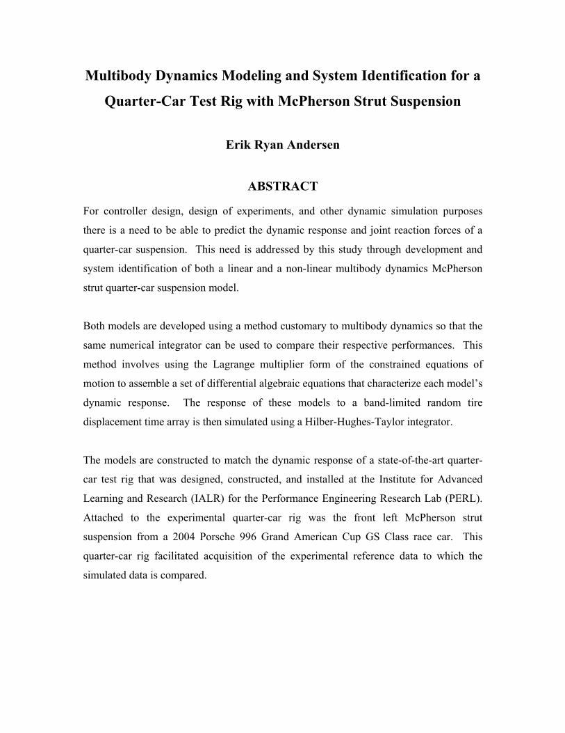
For controller design, design of experiments, and other dynamic simulation purposes

there is a need to be able to predict the dynamic response and joint reaction forces of a

quarter-car suspension. This need is addressed by this study through development and

system identification of both a linear and a non-linear multibody dynamics McPherson

strut quarter-car suspension model.

Both models are developed using a method customary to multibody dynamics so that the

same numerical integrator can be used to compare their respective performances. This

method involves using the Lagrange multiplier form of the constrained equations of

motion to assemble a set of differential algebraic equations that characterize each model’s

dynamic response. The response of these models to a band-limited random tire

displacement time array is then simulated using a Hilber-Hughes-Taylor integrator.

The models are constructed to match the dynamic response of a state-of-the-art quarter-

car test rig that was designed, constructed, and installed at the Institute for Advanced

Learning and Research (IALR) for the Performance Engineering Research Lab (PERL).

Attached to the experimental quarter-car rig was the front left McPherson strut

suspension from a 2004 Porsche 996 Grand American Cup GS Class race car. This

quarter-car rig facilitated acquisition of the experimental reference data to which the

simulated data is compared.

After developing these models their optimal parameters are obtained by performing

system identification. The performance of both models using their respective optimal

parameters is presented and discussed in the context of the basic linearity of the

experimental suspension.

Additionally, a method for estimating the loads applied to the experimental quarter-car

rig bearings is developed. Finally, conclusions and recommendations for future research

and applications are presented.

ACKNOWLEDGMENTS

I would like to thank Dr. Corina Sandu for taking the time to work with and guide me

through this thesis. Your patience and flexibility in atypical circumstances went above

and beyond any known standard. I would also like to thank Dr. Steve Southward for your

guidance and encouragement. Your willingness and ability to guide me through technical

issues I encountered during this work was incredibly helpful. Also, I would like to thank

Brendan Chan for your tutelage and for going beyond the call of duty to help me through

this process. Discussing the finer points of multibody dynamics over pizza made if all

the more enjoyable. I couldn’t have asked for a better team.

I would also like to thank Dr. Mary Kasarda for agreeing to be on my committee and

providing excellent feedback. Thanks are also due to Dr. Mehdi Ahmadian for

graciously and patiently steering me in the right direction.

To my mom, thank you for teaching and encouraging me to have the serenity to accept

the things I cannot change, the courage to change the things I can, and the wisdom to

know the difference. To my dad, thank you for providing unyielding stability and peace

of mind. Also, thank you for providing a constant address throughout my many moves.

To my brother, Peder, thank you for teaching me that we are only bounded by our

imagination.

To my grandmother, Elvira Andersen, thank you for exemplifying patience, tenacity, and

kindness. Your wisdom enriched all whose lives you touched.

To Victor Goldthorp, Elsie Goldthorp, Peder Andersen, Freda Sutton, Spencer Sutton,

Timothy Sutton, Leslie Jackson, and Beth Johnson, thank you all for the support and

balance you brought to me through this journey. Your humor and goodwill kept this ship

sailing.

I would also like to thank all of my friends in AVDL and PERL for giving these labs

personality and for the many laughs we shared. Best of luck to you all.

iv

CONTENTS ABSTRACT....................................................................................................................... ii

ACKNOWLEDGMENTS ................................................................................................ iv

LIST OF FIGURES .......................................................................................................... ix

LIST OF TABLES............................................................................................................ xi

LIST OF SYMBOLS .......................................................................................................xii

1. INTRODUCTION ....................................................................................................... 1

1.1 Motivation .......................................................................................................... 1

1.2 Objectives........................................................................................................... 2

1.3 Approach ............................................................................................................ 3

1.4 Outline................................................................................................................ 4

2. LITERATURE SEARCH ............................................................................................ 5

2.1 McPherson Strut ................................................................................................. 5

2.2 Quarter-car Modeling......................................................................................... 7

2.3 Simulation ........................................................................................................ 10

3. LABORATORY SETUP........................................................................................... 12

3.1 Lab Overview................................................................................................... 12

3.2 Quarter-car Rig................................................................................................. 12

3.3 Hydraulic Driving Equipment .......................................................................... 16

3.4 Electronic Driving and Measuring Equipment................................................. 17

3.5 Data Collection Procedure ............................................................................... 20

4. LINEAR QUARTER-CAR MODEL ........................................................................ 25

4.1 Introduction ...................................................................................................... 25

4.2 Coordinates....................................................................................................... 26

4.3 Degrees of Freedom ......................................................................................... 27

4.4 Kinematic Assumptions and Constraints ......................................................... 28

4.5 Driving Constraint............................................................................................ 28

v

4.6 Complete Constraint Vector............................................................................. 28

4.7 Acceleration Equations .................................................................................... 29

4.8 Applied Force Vector ....................................................................................... 31

4.8.1 Primary TSD ........................................................................................ 33

4.8.2 Tire TSD............................................................................................... 34

4.8.3 Sprung Mass Forces ............................................................................. 36

4.8.4 Unsprung Mass Forces ......................................................................... 36

4.8.5 Actuator Forces .................................................................................... 37

4.8.6 Complete Force Vector ........................................................................ 37

4.9 Mass Matrix...................................................................................................... 38

4.10 McPherson Strut Linear DAE .......................................................................... 38

5. LINEAR QUARTER-CAR MODEL SYSTEM IDENTIFICATION ...................... 39

5.1 Introduction ...................................................................................................... 39

5.2 Hilber-Hughes-Taylor DAE Integrator ............................................................ 39

5.3 System Identification........................................................................................ 40

5.4 Procedure.......................................................................................................... 41

5.5 Performance Measure....................................................................................... 44

5.6 Linear System Identification Results ............................................................... 44

6. NON-LINEAR QUARTER-CAR MODEL .............................................................. 47

6.1 Introduction ...................................................................................................... 47

6.2 Coordinates....................................................................................................... 47

6.3 Degrees of Freedom ......................................................................................... 48

6.4 Kinematic Assumptions ................................................................................... 49

6.5 Kinematic Constraints ...................................................................................... 49

6.5.1 Translational Joint ................................................................................ 50

6.5.2 Revolute Joint A................................................................................... 51

6.5.3 Revolute Joint B ................................................................................... 52

vi

6.5.4 Revolute-Translational Joint PQ .......................................................... 54

6.6 Driving Constraint............................................................................................ 57

6.7 Complete Constraint Vector............................................................................. 57

6.8 Acceleration Equations .................................................................................... 59

6.9 Applied Force Vector ....................................................................................... 60

6.9.1 Primary TSD ........................................................................................ 63

6.9.2 Tire TSD............................................................................................... 65

6.9.3 Sprung Mass Forces ............................................................................. 66

6.9.4 Control Arm Forces.............................................................................. 69

6.9.5 Unsprung Mass Forces ......................................................................... 70

6.9.6 Complete Force Vector ........................................................................ 72

6.10 Mass Matrix...................................................................................................... 73

6.11 McPherson Strut Non-Linear DAE .................................................................. 73

7. NON-LINEAR QUARTER-CAR MODEL SYSTEM IDENTIFICATION ............ 75

7.1 Introduction ...................................................................................................... 75

7.2 Simulation ........................................................................................................ 75

7.3 Procedure.......................................................................................................... 75

7.4 Performance Measure....................................................................................... 78

7.5 Non-Linear System Identification Results ....................................................... 78

7.6 Discussion ........................................................................................................ 80

8. LINEAR BEARING LOADS.................................................................................... 82

8.1 Introduction ...................................................................................................... 82

8.2 Joint Reaction Forces ....................................................................................... 82

8.3 Sprung Mass Force........................................................................................... 84

8.4 Bearing Force ................................................................................................... 88

9. CONCLUSIONS AND RECOMMENDATIONS .................................................... 91

9.1 Modeling .......................................................................................................... 91

vii

9.2 Load Estimation ............................................................................................... 91

9.3 Model Template ............................................................................................... 92

9.4 Conclusion........................................................................................................ 92

9.5 Recommendations for Future Research ........................................................... 92

REFERENCES ................................................................................................................ 94

Appendix A – Control Arm and Unsprung Mass Moments of Inertia ............................ 96

Appendix B – Bearing Loads with Simplified Constraints ........................................... 102

viii

LIST OF FIGURES

Figure 2-1 McPherson Strut Suspension............................................................................ 6

Figure 3-1 Lab Overview................................................................................................. 14

Figure 3-2 Quarter-car Rig............................................................................................... 15

Figure 3-3 Hydraulic Equipment ..................................................................................... 16

Figure 3-4 Lab Electronics............................................................................................... 17

Figure 3-5 Accelerometer Locations ............................................................................... 19

Figure 3-6 Accelerometer and Mounting Stud ................................................................ 20

Figure 3-7 LVDT Measured Pan Position vs. Time (0-8 Sec) ........................................ 22

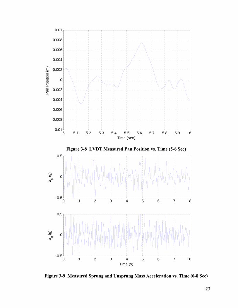
Figure 3-8 LVDT Measured Pan Position vs. Time (5-6 Sec) ........................................ 23

Figure 3-9 Measured Sprung and Unsprung Mass Acceleration vs. Time (0-8 Sec) ...... 23

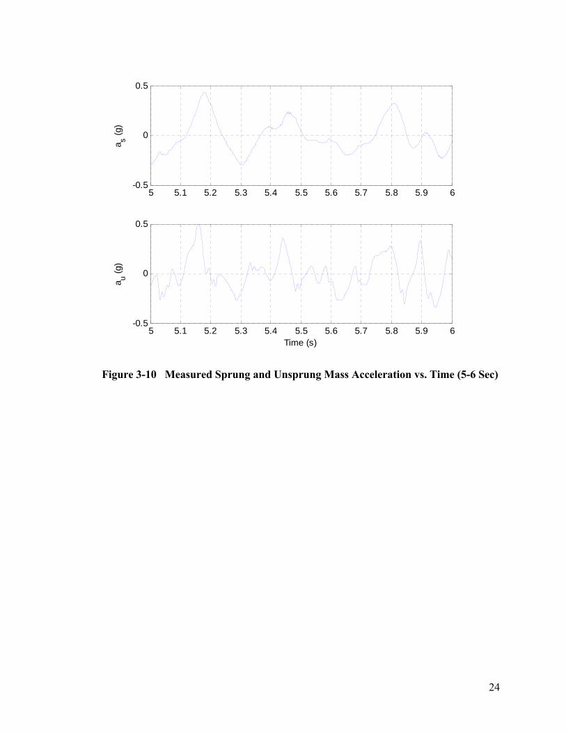
Figure 3-10 Measured Sprung and Unsprung Mass Acceleration vs. Time (5-6 Sec) ... 24

Figure 4-1 Linear Quarter-Car Model.............................................................................. 26

Figure 4-2 Linear Model Forces ...................................................................................... 32

Figure 4-3 Linear Model Primary TSD ........................................................................... 33

Figure 4-4 Linear Model Tire TSD.................................................................................. 35

Figure 4-5 Linear Model Sprung Mass Forces ................................................................ 36

Figure 4-6 Linear Model Unsprung Mass Forces ............................................................ 36

Figure 5-1 Linear Model Initial Parameter Estimates...................................................... 43

Figure 5-2 Linear Model Initial Conditions..................................................................... 43

Figure 5-3 Experimental vs. Simulated Linear Model Acceleration with Non-Optimized

Parameters......................................................................................................................... 45

Figure 5-4 Experimental vs. Simulated Linear Model Acceleration with Optimized

Parameters......................................................................................................................... 46

Figure 6-1 Non-Linear Quarter-Car Model ..................................................................... 48

Figure 6-2 Non-Linear Model Joints ............................................................................... 49

Figure 6-3 Translational Joint.......................................................................................... 50

Figure 6-4 Revolute Joint A............................................................................................. 52

Figure 6-5 Revolute Joint B............................................................................................. 54

Figure 6-6 Revolute-Translational Joint .......................................................................... 55

Figure 6-7 Non-Linear Model TSDs................................................................................ 61

ix

Figure 6-8 Non-Linear Model Primary TSD ................................................................... 63

Figure 6-9 Non-Linear Model Tire TSD ......................................................................... 65

Figure 6-10 Non-Linear Model Sprung Mass Forces ...................................................... 67

Figure 6-11 Non-Linear Model Control Arm Force ........................................................ 69

Figure 6-12 Non-Linear Model Unsprung Mass Forces.................................................. 70

Figure 7-1 Non-Linear Model Initial Parameter Estimates ............................................. 76

Figure 7-2 Non-Linear Model Initial Conditions............................................................. 77

Figure 7-3 Non-Linear Model Geometric Constants ....................................................... 77

Figure 7-4 Experimental vs. Simulated Non-Linear Model Acceleration with Non-

Optimized Parameters....................................................................................................... 79

Figure 7-5 Experimental vs. Simulated Non-Linear Model Acceleration with Optimized

Parameters......................................................................................................................... 80

Figure 7-6 Simulated Strut Arm Angle (degrees)............................................................ 81

Figure 8-1 Equivalent Translational Joint Depictions ..................................................... 82

Figure 8-2 Sprung Mass Normal Force and Torque ........................................................ 87

Figure 8-3 Simplified Quarter-car Bearing Reactions ..................................................... 89

Figure 8-4 Upper and Lower Quarter-car Bearing Forces................................................ 89

x

LIST OF TABLES

Table 2-1 Literature Search Matrix.................................................................................... 5

Table 3-1 Filtering Matrix ............................................................................................... 21

Table 5-1 Linear Model Optimal Parameters .................................................................. 45

Table 7-1 Non-Linear Model Optimal Parameters .......................................................... 80

Table 8-1 Non-Linear Model Optimized Parameters For Load Prediction ..................... 86

xi

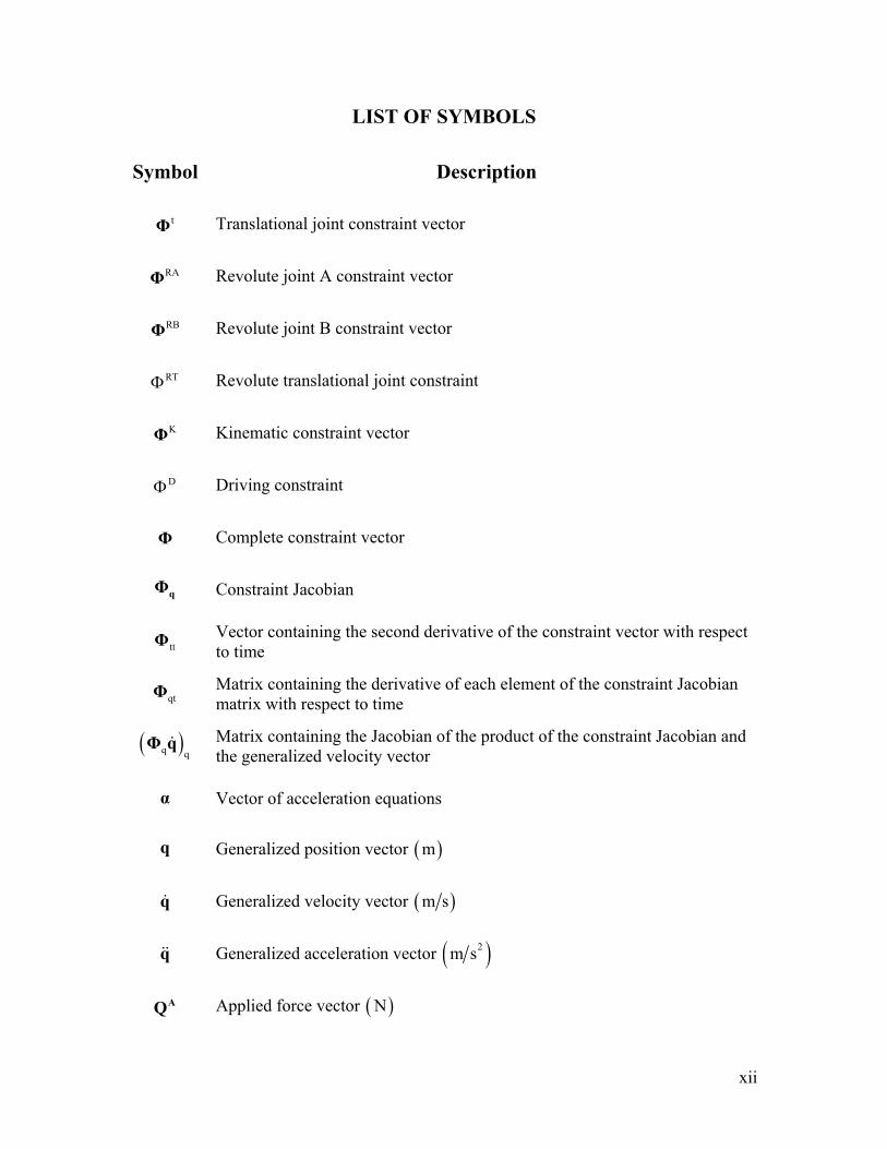
LIST OF SYMBOLS

Symbol Description

tΦ

Φ

Φ

Φ

Φ

Φ

Φ

tt

α

Translational joint constraint vector

RA Revolute joint A constraint vector

RB Revolute joint B constraint vector

RT Revolute translational joint constraint

K Kinematic constraint vector

D Driving constraint

Complete constraint vector

qΦ Constraint Jacobian

Φ Vector containing the second derivative of the constraint vector with respect to time

qtΦ Matrix containing the derivative of each element of the constraint Jacobian matrix with respect to time

( )q qΦ q& Matrix containing the Jacobian of the product of the constraint Jacobian and

the generalized velocity vector

Vector of acceleration equations

q Generalized position vector ( )m

q& Generalized velocity vector ( )m s

q&& Generalized acceleration vector ( )2m s

AQ Applied force vector ( )N

xii

pk Primary suspension stiffness ( )N/m

pn Primary suspension damping ( )( )N/ m s

tk Tire stiffness ( )N/m

tn Tire damping ( )( )N/ m s

PF

F

λ

Primary TSD force ( )N

T Tire TSD force ( ) N

Vector of Lagrange multipliers

isφ , icφ Short-hand notation for sine and cosine of iφ

X , Y Global reference frame

Sr Global representation of the vector from the global origin to the sprung mass CG ( ) m

Sx , Sy Global representation of the sprung mass position – components of ( ) Sr m

Cr Global representation of the vector from the global origin to the control arm CG ( ) m

Cx , Cy Global representation of the control arm position – components of ( ) Cr m

Ur Global representation of the vector from the global origin to the unsprung mass CG ( ) m

Ux , Uy Global representation of the unsprung mass position – components of

Ur

( )m

Ay Global representation of the wheel pan position ( )m

Sx ′ , Sy ′ Local reference frame embedded at the sprung mass CG

Cx ′ , Cy ′ Local reference frame embedded at the control arm CG

xiii

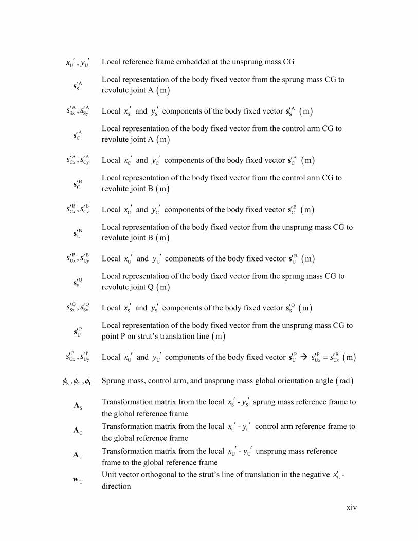
Ux ′ , Uy ′ Local reference frame embedded at the unsprung mass CG

AS′s

Local representation of the body fixed vector from the sprung mass CG to revolute joint A ( )m

ASxs′ , A

Sys′ Local Sx ′ and components of the body fixed vector Sy ′ AS′s ( )m

AC′s

Local representation of the body fixed vector from the control arm CG to revolute joint A ( )m

ACxs′ , A

Cys′ Local Cx ′ and components of the body fixed vector Cy ′ AC′s ( ) m

BC′s

Local representation of the body fixed vector from the control arm CG to revolute joint B ( ) m

BCxs′ , B

Cys′ Local Cx ′ and components of the body fixed vector Cy ′ BC′s ( )m

BU′s

Local representation of the body fixed vector from the unsprung mass CG to revolute joint B ( ) m

BUxs′ , B

Uys′ Local Ux ′ and components of the body fixed vector Uy ′ BU′s ( )m

QS′s

Local representation of the body fixed vector from the sprung mass CG to revolute joint Q ( )m

QSxs′ , Q

Sys′ Local Sx ′ and components of the body fixed vector Sy ′ QS′s ( )m

PU′s

Local representation of the body fixed vector from the unsprung mass CG to point P on strut’s translation line ( )m

PUxs′ , P

Uys′ Local Ux ′ and components of the body fixed vector Uy ′ PU′s P B

Ux Uxs s′ ′= ( )m

Sφ , Cφ , Uφ Sprung mass, control arm, and unsprung mass global orientation angle ( ) rad

SA Transformation matrix from the local Sx ′ - Sy ′ sprung mass reference frame to the global reference frame

CA Transformation matrix from the local Cx ′ - Cy ′ control arm reference frame to the global reference frame

UA Transformation matrix from the local Ux ′ - Uy ′ unsprung mass reference frame to the global reference frame

Uw Unit vector orthogonal to the strut’s line of translation in the negative Ux′ -direction

xiv

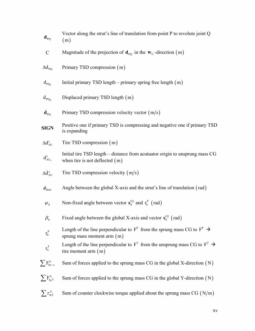
PQd Vector along the strut’s line of translation from point P to revolute joint Q

( )m

C Magnitude of the projection of in the -direction PQd Uw ( )m

PQdΔ Primary TSD compression ( )m

IPQd Initial primary TSD length – primary spring free length ( )m

DPQd Displaced primary TSD length ( )m

PQd& Primary TSD compression velocity vector ( )m s

SIGN Positive one if primary TSD is compressing and negative one if primary TSD is expanding

yAUdΔ Tire TSD compression ( )m

I

yAUd

Initial tire TSD length – distance from acutuator origin to unsprung mass CG when tire is not deflected ( )m

yAUdΔ& Tire TSD compression velocity ( )m s

Strutφ Angle between the global X-axis and the strut’s line of translation ( ) rad

Sψ Non-fixed angle between vector QS′s and P

Sr ( )rad

Sβ Fixed angle between the global X-axis and vector QS′s ( )rad

PSr

Length of the line perpendicular to from the sprung mass CG to sprung mass moment arm

PF PF( )m

TUr

Length of the line perpendicular to from the unsprung mass CG to tire moment arm

TF TF( )m

ASxF →∑ Sum of forces applied to the sprung mass CG in the global X-direction ( )N

ASyF ↑∑ Sum of forces applied to the sprung mass CG in the global Y-direction ( )N

ASτ∑ Sum of counter clockwise torque applied about the sprung mass CG ( )N m

xv

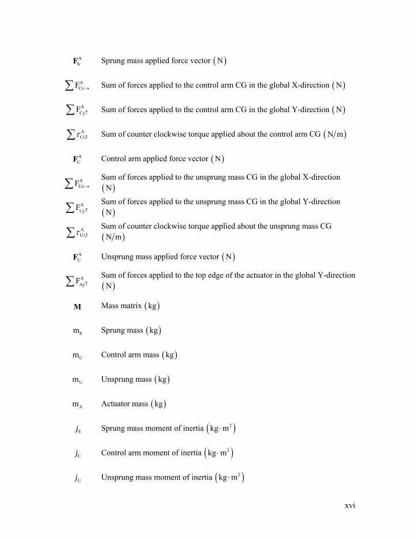
ASF Sprung mass applied force vector ( )N

ACxF →∑ Sum of forces applied to the control arm CG in the global X-direction ( ) N

ACyF ↑∑ Sum of forces applied to the control arm CG in the global Y-direction ( ) N

ACτ∑ Sum of counter clockwise torque applied about the control arm CG ( )N m

ACF Control arm applied force vector ( )N

AUxF →∑

Sum of forces applied to the unsprung mass CG in the global X-direction ( )N

AUyF ↑∑

Sum of forces applied to the unsprung mass CG in the global Y-direction ( )N

AUτ∑

Sum of counter clockwise torque applied about the unsprung mass CG ( )N m

AUF Unsprung mass applied force vector ( )N

AAyF ↑∑

Sum of forces applied to the top edge of the actuator in the global Y-dir( )N

ection

M Mass matrix ( ) kg

Sm Sprung mass ( ) kg

Cm Control arm mass ( ) kg

Um Unsprung mass ( ) kg

Am Actuator mass ( )kg

Sj Sprung mass moment of inertia ( )2kg m⋅

Cj Control arm moment of inertia ( )2kg m⋅

Uj Unsprung mass moment of inertia ( )2kg m⋅

xvi

g Acceleration due to gravity ( )2m s

SR Sprung mass performance ratio ( )dB

UR Unsprung mass performance ratio ( )dB

ki′′F Joint reaction force ( )N

iC Rotation matrix that transforms vectors in the joint reference frame ‘i’ to the body reference frame

iA Rotation matrix that transforms vectors in the body reference frame ‘i’ to the global reference frame

irkΦ Partial Jacobian associated with constraint force and translational coordinates

kλ Vector of Lagrange multipliers associated with joint k

kiτ ′′ Joint reaction torque ( )N m

Pi′s Vector from body i’s local reference frame to the joint reference frame ( )m

iB Derivative of the rotation matrix with respect to its angle

i

kφΦ Partial Jacobian associated with constraint torque and rotational coordinate

S′′F Sprung mass translational joint reaction force ( )N

SC Sprung mass rotation matrix that transforms vector SP′s in the translational

joint reference frame to the sprung mass reference frame

SrΦ Jacobian of sprung mass constraint vector with respect to translational

coordinates

Sτ ′′ Sprung mass joint reaction torque ( )N m

SP′s

Vector from the sprung mass CG to the translational joint reference frame ( )m

SB Derivative of with respect to SA Sφ

xvii

xviii

SφΦ Jacobian of sprung mass constraint vector with respect to the rotational

coordinate

SxF → Constraint force acting on the sprung mass CG ( )N

Sτ Constraint torque acting on the sprung mass ( )N m

BUF , BLF Upper and lower bearing reaction forces ( )N

ul , llDistance to upper and lower bearing reaction forces from sprung mass CG

( )m

1. INTRODUCTION

This thesis addresses modeling, system identification, and various design aspects related

to a McPherson strut suspension. As such, it has both theoretical and experimental

components. A state-of-the-art quarter-car test rig with the front left McPherson strut

suspension from a 2004 Porsche 996 Grand American Cup GS Class race car provides

the experimental counterpoint to the theoretical models developed herein.

1.1 Motivation

Active and semi-active suspensions have the potential to increase vehicular comfort,

performance, and safety (Gillespie [1]). For example, an active suspension may increase

comfort by reducing the acceleration experienced by the sprung mass and, hence, by the

vehicle occupants. An active suspension may increase the vehicle performance and

safety of its occupants by minimizing the tire-pavement normal force fluctuation. By

stabilizing this force, the dips in lateral adhesion associated with lower-than-usual tire-

pavement normal force can be avoided, which facilitates predictable, safe, and high

performance handling characteristics. The effectiveness of active and semi-active

suspensions is, in some cases, partly attributed to the controller’s ability to predict the

suspension’s dynamic response. Thus, an accurate suspension model is necessary for the

controller to predict the suspension’s response.

Computer based quarter-car test models are often employed in vehicle dynamics studies

as simplified and well-understood systems for such uses as testing new control strategies,

designing new suspension systems, and analyzing ride dynamics. When available,

quarter-car rigs are used to obtain relevant experimental data. A quarter-car test rig is an

experimental platform which attempts to replicate the dynamics of one corner of a car.

Having an accurate computer model of the test rig used is very valuable since it gives the

researcher more flexibility in experimenting with various scenarios in the virtual world,

helps design experiments, and helps perform extensive analysis. In this study the focus

was on modeling and performing system identification on a quarter-car rig that, unlike

typical quarter-car rigs, contains a full suspension system. The suspension under study is

1

a McPherson strut suspension, but the quarter-car test rig, as it was designed, is capable

of accommodating a multitude of different suspensions. As such, care must be taken so

that a suspension that is capable of producing dynamic loads higher than that which the

quarter-car test rig’s linear bearings are rated for is not used. This load, termed here as

the normal load, is that which is applied to the sprung mass plate’s linear bearings

perpendicular to the side which the suspension attaches to. Multibody dynamics models

are capable of estimating the dynamic normal loads applied to the quarter-car rig’s

sprung mass, which provides additional motivation for the present study.

It is foreseeable that different suspensions will be used on the quarter-car test rig. It is

expected that a non-linear quarter-car dynamics model that accurately simulates the

original system and accounts for its constraints will provide more accurate results and

offer increased capabilities compared to traditional linear single-axis quarter-car models.

The term non-linear refers to the fact that, in addition to simulating its linear motion, the

non-linear model accounts for the suspension’s angular displacements. In order to take

advantage of its increased accuracy and special capabilities, the quarter-car model must

be clearly defined and easy to adapt to future changes in the system.

1.2 Objectives

The first objective is to formulate linear and non-linear multibody dynamic McPherson

strut suspension models and compare their accuracy. For this study, the most accurate

model is defined as the model that best predicts the experimental sprung mass and

unsprung mass vertical accelerations.

The second objective is to use the non-linear multibody dynamics model to estimate the

dynamic normal loads applied to the quarter-car rig’s sprung mass plate and bearings.

The third objective is to clearly describe the formulation of the multibody dynamics non-

linear quarter-car McPherson strut suspension model so that it can be used as a template

for future use.

2

1.3 Approach

The non-linear motion of vehicular suspensions is often represented with a linear model.

Among the reasons for such a modeling choice are ease and familiarity with linear

modeling. Also, for non-linear suspensions that possess nearly linear motion, a linear

model may represent the suspension’s dynamics accurately enough for its intended

application. However, the more non-linear a suspension’s motion is, the less accurate a

linear model is at predicting its dynamics. For moderately to highly non-linear

suspensions a linear model may not be suitable for predicting dynamic response.

A McPherson strut suspension possesses non-linear motion, in part because its strut and

control arm rotate. One way of quantifying the degree of non-linearity exhibited in a

McPherson strut suspension is by examining its strut angle change throughout its range of

motion. A race car-derived McPherson strut suspension, by design, does not facilitate

much suspension travel and thus is minimally non-linear. Bearing this in mind, the

approach used to determine the most accurate McPherson strut suspension model was to

develop a linear model and a non-linear model using the same multibody dynamics

method, and compare their respective performances. The performance comparison was

carried out using optimal parameters found through system identification for each

respective model.

Motion of the non-linear quarter-car model is completely described by a set of ordinary

differential equations and algebraic equations associated with the constraints, leading to a

set of differential algebraic equations (DAE) that must be solved to obtain system

dynamics. In addition to obtaining the accelerations for the set of generalized coordinates

used, solving the DAE will also yield Lagrange multipliers introduced to account for the

algebraic constraints. These Lagrange multipliers are associated with the joint reaction

forces. The Lagrange multipliers associated with the translational and rotational

kinematic constraints of the sprung mass provide information about the normal reaction

force and the torque in the quarter-car rig’s bearings. Thus the approach used to estimate

the dynamic normal loads was to calculate them from the translational joint reaction force

formula that utilizes Lagrange multipliers produced by the DAE simulation.

3

The DAE describing the non-linear multibody dynamics of the quarter-car McPherson

strut suspension is the mathematical basis needed to simulate and predict the dynamic

response of the non-linear quarter-car test rig. A detailed description of the DAE system

and the method used to solve it is provided in this study.

1.4 Outline

Chapter 2 presents results of the literature search. Chapter 3 explains the experimental

quarter-car setup and the procedure used to collect data, and also contains experimental

results. Chapter 4 develops the linear model approximation of the quarter-car McPherson

strut suspension model. Chapter 5 presents background information on the integrator

used to solve the DAE and on the system identification method used. The results of the

system identification of the linear quarter-car McPherson strut suspension model

developed in Chapter 4 are also presented here. Chapter 6 develops the non-linear

multibody dynamics quarter-car McPherson strut suspension model. Chapter 7 discusses

results from the system identification of the non-linear quarter-car McPherson strut

suspension model developed in Chapter 6. Chapter 8 discusses the method used to

determine the dynamic normal loads applied to the quarter-car rig’s sprung mass. This

chapter also presents bearing normal load results. Chapter 9 summarizes this work and

provides recommendations for future research.

4

2. LITERATURE SEARCH

This chapter presents a literature review related to McPherson strut suspension history

and applications, multibody dynamics and quarter-car modeling, and simulation. Several

sources were searched in conjunction with pertinent key words. Because both

Macpherson and McPherson strut are popular spellings for this type of suspension, both

were used in this search. Table 2-1 lists the number of articles found at each source

containing these keywords:

Table 2-1 Literature Search Matrix

ANTE: Abstracts in New Technologies and Engineering (DB) 3/4 0/0 0/0 2/0 2/0Engineering Village Compendex, Inspec & NTIS (DBs) 27/25 2/0 0/0 1/1 2/0CSA Technology (DB) 19/14 0/0 0/0 4/1 2/0Mechanical & Transportation Engineering Abstracts (DB) 11/4 0/0 0/0 2/0 1/0SAE Technical Papers (DB) 13/51 0/0 0/0 1/4 0/0Virginia Tech Addision Book Search 0/0 0/0 0/0 0/0 0/0

WorldCat dissertations and theses 4/0 0/0 0/0 0/0 0/0

Database (DB), Journal, or Thesis Source Quarter car &

M

acpherson/ McPherson

strut

Macpherson/ M

cPherson strut

Macpherson/ M

cPherson strut m

odel

McPherson strut

modeling

Macpherson/ M

cPherson strut &

multibody

dynamics

Key Words

2.1 McPherson Strut

This section provides a historical and applications perspective on the McPherson strut

suspension.

The McPherson strut suspension, designed in the late 1940s by Earl Steele Macpherson,

was first used on the 1949 Ford Vedette (Gilles [2]). As such, it is a relatively new

suspension configuration. Mantaras [3] states that the vast majority of current small- and

medium-sized cars use this configuration. The McPherson strut suspension configuration

5

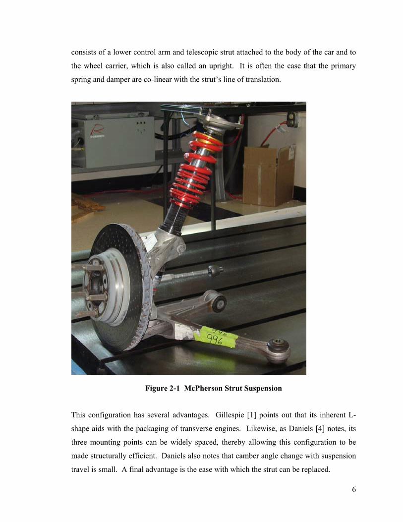
consists of a lower control arm and telescopic strut attached to the body of the car and to

the wheel carrier, which is also called an upright. It is often the case that the primary

spring and damper are co-linear with the strut’s line of translation.

Figure 2-1 McPherson Strut Suspension

This configuration has several advantages. Gillespie [1] points out that its inherent L-

shape aids with the packaging of transverse engines. Likewise, as Daniels [4] notes, its

three mounting points can be widely spaced, thereby allowing this configuration to be

made structurally efficient. Daniels also notes that camber angle change with suspension

travel is small. A final advantage is the ease with which the strut can be replaced.

6

Nevertheless, this type of suspension configuration also has some disadvantages. From a

packaging standpoint, although beneficial for transverse engines, this configuration’s

high installation height limits the designer’s ability to lower the hood height [1]. From a

performance standpoint, Daniels notes that the effect of the rolling force increases the

further the body rolls due to the roll center migration incurred with this suspension.

Daniels also notes that roll center migration on a double wishbone suspension creates no

serious problem [4]. Another performance compromise Milliken [5] mentions is that

McPherson strut suspensions lose negative camber when the suspension travels upward.

Despite these disadvantages, manufacturers such as Porsche and BMW use this

suspension to great effect in their road racing efforts. Likewise, consumer car makers

such as Toyota and General Motors use them effectively on their passenger vehicles.

2.2 Quarter-car Modeling

This section discusses multibody dynamics background, methods, and previous work in

quarter-car model construction.

Selection of the coordinate system is the first step in multibody dynamics modeling. De-

Jalon [6] discusses the implementation, advantages, and disadvantages associated with

relative, reference point, and natural 2D coordinates. Relative coordinates describe the

relative motion between two adjoining elements. For example, a revolute joint would be

described by the angle between the elements it connects and a translational joint by the

distance between connected elements. Constraint equations are generated from the vector

equations that close kinematic loops. This system uses a low number of coordinates and

is especially apt at describing open-chain configurations. However, mathematical

formulation can be problematic, and although few coordinates are used the equations of

motion they create can be computationally expensive. Additionally, pre- and post-

processing is required to determine each joint’s absolute motion.

7

Reference point coordinates specify element position and orientation by embedding a

local coordinate system in that element, specifying the X-Y position of the local

coordinate origin, and orientation angle between a local axis and the global inertial axis.

Often local axes are denoted with a prime, for example ′ or yx ′ . Constraint equations

are written based on the type of motion each joint allows between adjacent elements. For

example, a revolute joint would constrain both X and Y translation. Because the position

and orientation of each element is directly specified, little pre- and post-processing are

necessary to determine each joint’s absolute motion. The main disadvantage of this

system is that the large number of coordinates it requires can lengthen simulation time.

Natural coordinates specify two points on a body to determine its position and orientation

in space. Constraints are written by rigid body condition (that is, the distance between

two points on a rigid body is constant) or by joint constraints. This system is

advantageous because it eliminates angular coordinates, and little pre- or post-processing

is needed. However, this system requires a larger number of coordinates than relative

coordinates would.

For this thesis, reference point coordinates are used because of their advantages. The

kinematic and dynamic approach used in this study, including kinematic joint constraints,

formulation of the differential equations of motion, and constraint reaction forces,

follows the methodology described by Haug [7].

A ride frequency of approximately 4 Hz was observed from the experimental McPherson

strut suspension. Milliken puts this result in context by providing useful insight as to

what ride frequencies to expect from road-circuit race cars that employ aerodynamic

down force packages. He mentions that ride frequencies between 3.0 and 5.0 Hz have

proven successful for race cars with significant aerodynamic down force and that the

front axle’s ride frequency is higher than the rear. Given that the experimental

suspension is from the front of a Porsche 996 race car that employs an aerodynamic down

force package, the observed ride frequency of approximately 4 Hz is within expectation.

8

Milliken also provides insight on how to use the observed ride frequency to estimate the

total static deflection of the primary suspension and tire. Total static deflection is defined

here as the change in vertical position of the sprung mass CG relative to the inertial

reference frame that occurs when the sprung mass is placed on and statically supported

by the suspension. Milliken presents the relationship between the natural ride frequency

and static wheel deflection as:

( )188 cyc min.xnω =

n

(2.1)

In this equation ω is the ride natural frequency in cycles per minute and x is the static

wheel deflection in inches. Changing the ride natural frequency from units of cycles per

minute to cycles per second this equation becomes:

188 cyc min. 3.13 cycmin. 60 sec. sec.x xnω

⎛ ⎞⎛ ⎞ ⎛ ⎞= =⎜ ⎟⎜ ⎟ ⎜ ⎟⎝ ⎠⎝ ⎠ ⎝ ⎠

(2.2)

Rearranging this equation, the static deflection given a particular ride frequency is:

( )2

3.13x innω

⎛ ⎞= ⎜ ⎟⎝ ⎠

(2.3)

Given the observed experimental ride frequency of approximately 4 Hz, the total static

deflection this equation predicts is:

( )23.13x 0.61 in

4⎛ ⎞= =⎜ ⎟⎝ ⎠

(2.4)

9

In meters the total static deflection is:

( )( )( ) ( )0.0254 m

x 0.61 in 0.0155 m1 in

= × = (2.5)

Since the strut’s line of translation is essentially along the unsprung mass’s locus and thus

the installation ratio is essentially 1 to 1, this static deflection provides an estimation of

the sum of initial strut and tire compression used in system identification.

Prior work in quarter-car model construction and control has also been reviewed.

Rahnejat [8] discusses the formulation and analysis of a simplified multibody dynamics

2D McPherson strut suspension model. Gillespie [1] develops a linear quarter-car model

to describe vehicle response properties such as sprung mass isolation and transmissibility.

Inman [9] develops a base excitation model that can be used to represent a quarter-car

suspension. Five semi-active control policies are tested on a full-scale 2 degree-of-

freedom quarter-car system incorporating a magneto-rheological damper in Goncalve’s

[10] experimental study. Mantaras [3] presents a set of kinematic constraints used to

model a 3D McPherson strut suspension.

2.3 Simulation

This section discusses literature related to the simulation of multibody systems.

Once a multibody dynamics system is modeled with a set of differential algebraic

equations of motion (DAE), the system can be simulated. There are several methods for

solving DAE such as the Runge-Kutta algorithms discussed by Owren [11] and Laurent

[12]. The method used in this thesis is the Hilber-Hughes-Taylor (HHT) method

discussed by Negrut [13] and Cardona [14, 15]. This method was chosen to solve and

simulate the non-linear model because, according to Negrut, the combination of

numerical damping, A-stability, and second order accuracy make the HHT method

attractive for solving non-linear kinematically constrained multibody dynamics DAE.

10

Burden [16] defines a numerical method as A-stable if “its region R of absolute stability

contains the entire left half-plane.” For consistency, this method was also used to

simulate the linear model.

There are several examples of prior work on correlating experimental and dynamically

simulated suspensions. Trom [17] developed a multibody dynamics model of a mid-

sized passenger car with front McPherson strut suspension in Dynamic Analysis and

Design System (DADS) software. Dynamic simulations with this model are compared to

corresponding experimental data. Park [18] used model data from Salaani [19] to create

a full vehicle ADAMS simulation. This paper addressed how to refine kinematic steering

and suspension models using measurement data. Ozdalyan [20] developed an ADAMS

suspension model to replicate a Peugeot 605 McPherson strut suspension that provides

insight into how suspension parameters change in relation to each other. The wheel rate,

camber angle, caster angle, steer angle, and track change with suspension travel is

predicted in ADAMS and compared to the same experimentally-measured values

obtained from the Peugeot. For this particular experimental McPherson strut suspension,

the wheel rate, camber angle, caster angle, steer angle, and track changed approximately

3200 N/mm, 1.05 degrees, 0.4 degrees, 0.5 degrees, and 16 mm, respectively, over 120

mm of suspension travel. This work provides evidence that a McPherson strut’s change

in camber is much larger than its change in caster. This evidence supports the notion that

the majority of the kinematic non-linearity in a McPherson strut suspension can be

captured using a front view 2D multibody dynamics model.

11

3. LABORATORY SETUP

This chapter explains the experimental quarter-car test rig setup and the procedure used

to collect data, and presents experimental results.

3.1 Lab Overview

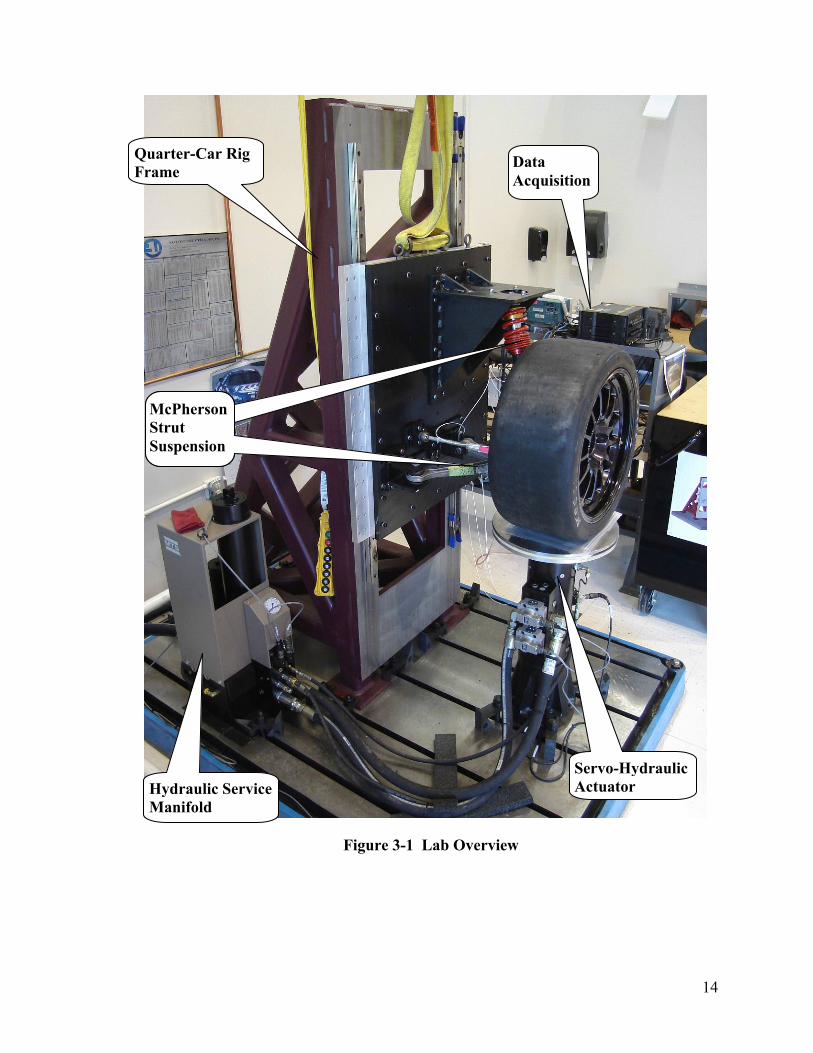
Figure 3-1 shows an overview of the physical quarter-car rig, hydraulic actuation

equipment, and electronic equipment used in the lab. Over the course of 2006, a state-of-

the-art quarter-car test rig was designed, constructed, and installed at the Institute for

Advanced Learning and Research (IALR) for the Performance Engineering Research Lab

(PERL). The rig has the potential to be used as a test bed for vehicular suspensions

ranging from lightweight race cars to heavy off-road High-Mobility Multipurpose

Wheeled Vehicles (HMMWV). This thesis used the front left McPherson strut

suspension from a 2004 Porsche 996 Grand American Cup GS Class race car attached to

the rig for experimental results. Sections below describe the experimental setup.

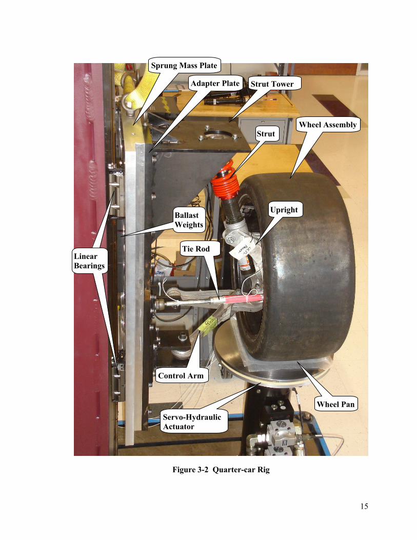
3.2 Quarter-car Rig

Figure 3-2 shows details of the quarter-car rig including the stationary frame, sprung

mass, and unsprung mass. The stationary frame includes the quarter-car rig frame (most

of which is painted in maroon) and the linear guides. The linear guides are equipped with

NSK LH35 series linear bearings capable of supporting a 61,385 N dynamic normal load

and 1,519 N-m static moment.

The sprung mass is defined here as the mass that is supported by the primary-ride spring.

The sprung mass plate, adapter plate, and strut tower constitute the bulk of the sprung

weight. Ballast weights were added to the sprung mass plate to approximate the left front

corner weight of a Porsche 996 race car.

The unsprung mass is defined here as the mass that is not supported by the primary-ride

spring. The strut and wheel assemblies constitute the bulk of the unsprung weight. The

12

strut assembly includes the main and tender springs, damper, and upright. The wheel

assembly is attached to the upright and consists of the brake disk, wheel, and tire.

Suspension geometry was adjusted such that it matched the actual 996 geometry.

Camber, caster, toe, and ride height were all brought within ranges found on the actual

996 race car.

Although at the time of this writing direct measurement of the rig’s total corner weight

was not possible, it has been estimated at 286 kg. This estimation is based on direct

measurement of suspension parts and computer solid modeling estimation of the sprung

mass components.

13

Quarter-Car Rig Frame Data

Acquisition

McPherson

Strut

S i

McPherson Strut Suspension

Servo-Hydraulic Actuator Hydraulic Service

Manifold

Figure 3-1 Lab Overview

14

Wheel AssemblyStrut

Adapter Plate

Sprung Mass Plate

Strut Tower

Linear

Guides

Linear Bearings

Upright Ballast Weights

Tie Rod

Servo-Hydraulic Actuator

Control Arm

Wheel Pan

Figure 3-2 Quarter-car Rig

15

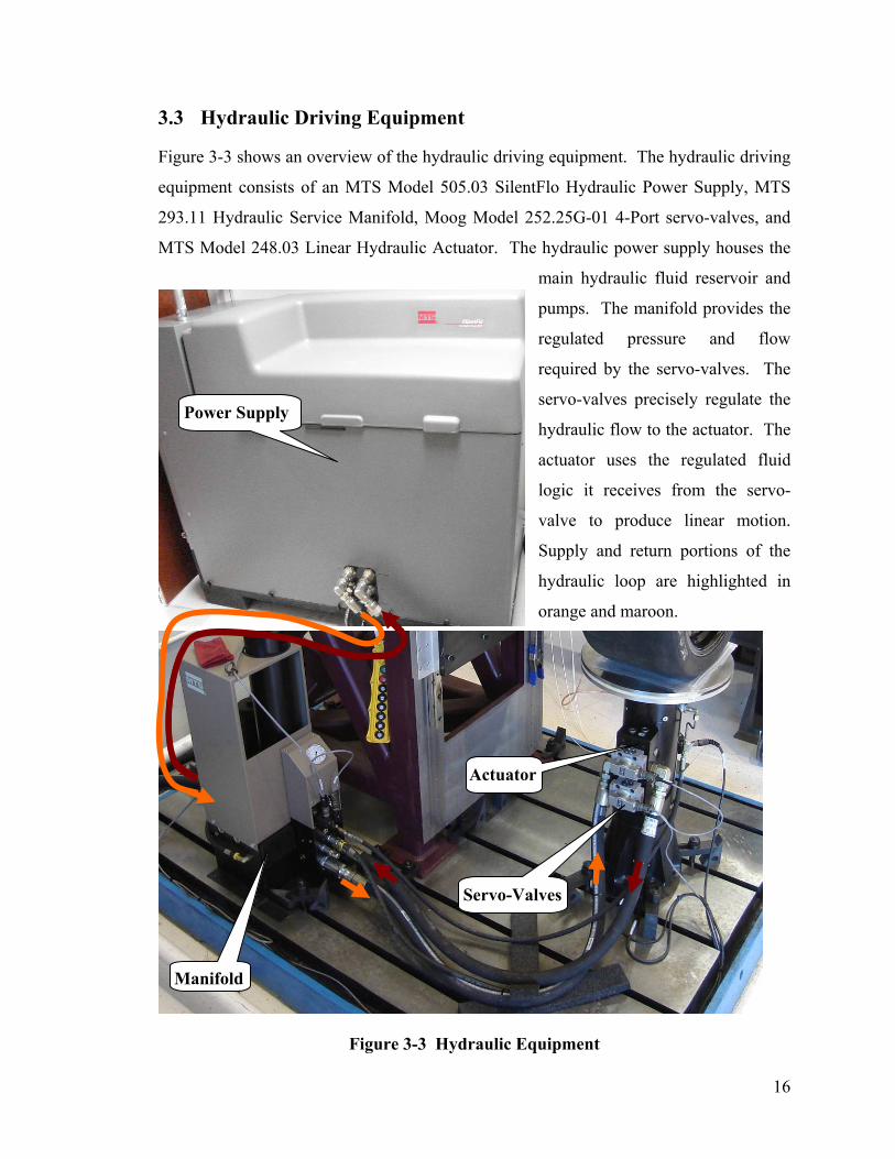
3.3 Hydraulic Driving Equipment

Figure 3-3 shows an overview of the hydraulic driving equipment. The hydraulic driving

equipment consists of an MTS Model 505.03 SilentFlo Hydraulic Power Supply, MTS

293.11 Hydraulic Service Manifold, Moog Model 252.25G-01 4-Port servo-valves, and

MTS Model 248.03 Linear Hydraulic Actuator. The hydraulic power supply houses the

main hydraulic fluid reservoir and

pumps. The manifold provides the

regulated pressure and flow

required by the servo-valves. The

servo-valves precisely regulate the

hydraulic flow to the actuator. The

actuator uses the regulated fluid

logic it receives from the servo-

valve to produce linear motion.

Supply and return portions of the

hydraulic loop are highlighted in

orange and maroon.

Power Supply

Actuator

Servo-Valves

Manifold

Figure 3-3 Hydraulic Equipment

16

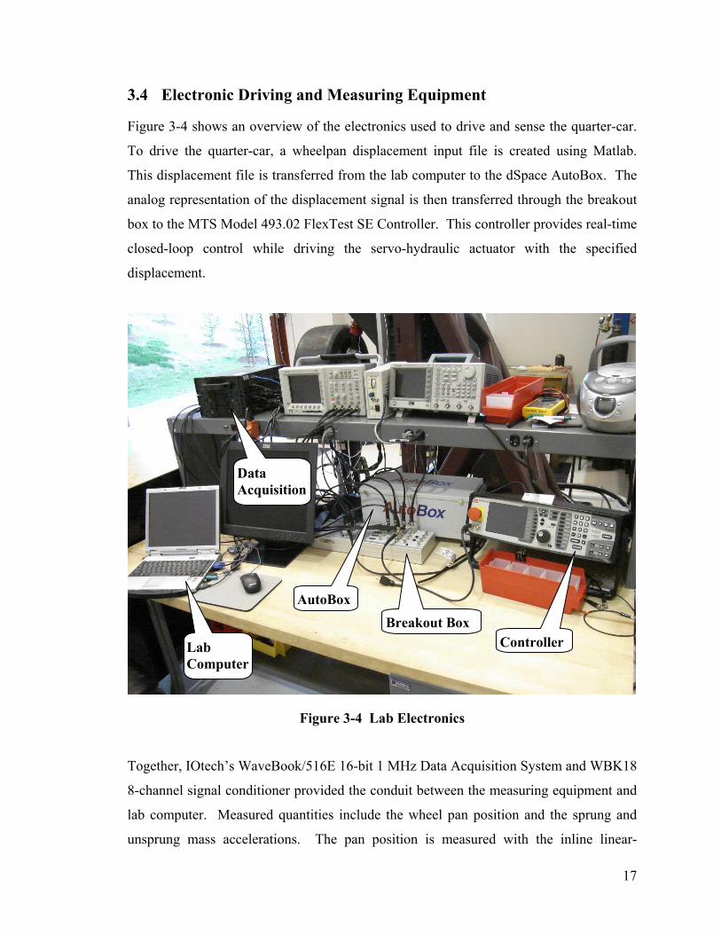
3.4 Electronic Driving and Measuring Equipment

Figure 3-4 shows an overview of the electronics used to drive and sense the quarter-car.

To drive the quarter-car, a wheelpan displacement input file is created using Matlab.

This displacement file is transferred from the lab computer to the dSpace AutoBox. The

analog representation of the displacement signal is then transferred through the breakout

box to the MTS Model 493.02 FlexTest SE Controller. This controller provides real-time

closed-loop control while driving the servo-hydraulic actuator with the specified

displacement.

Data Acquisition

Lab Computer

AutoBox

Controller Breakout Box

Figure 3-4 Lab Electronics

Together, IOtech’s WaveBook/516E 16-bit 1 MHz Data Acquisition System and WBK18

8-channel signal conditioner provided the conduit between the measuring equipment and

lab computer. Measured quantities include the wheel pan position and the sprung and

unsprung mass accelerations. The pan position is measured with the inline linear-

17

variable displacement transducer (LVDT) built into the hydraulic actuator. The

accelerations were measured using PCB Piezotronic Model 333B40 10-g accelerometers.

These piezoelectric accelerometers were calibrated to approximately 0.5 mV/g. Figure 3-

5 shows where the accelerometers are located on the sprung mass and unsprung mass.

The accelerometers are hard mounted to the sprung and unsprung masses using the small

stud in Figure 3-6.

18

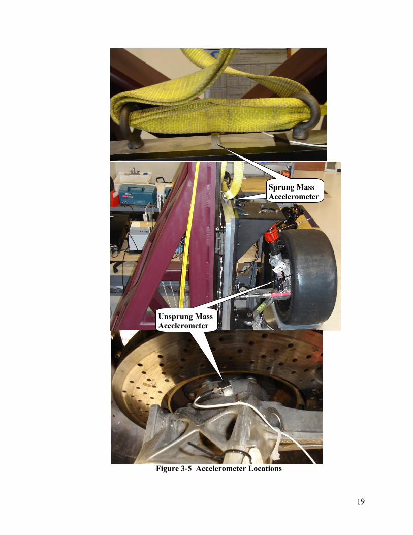
Sprung Mass

A l t

Sprung Mass Accelerometer

Unsprung

M

Unsprung Mass Accelerometer

Figure 3-5 Accelerometer Locations

19

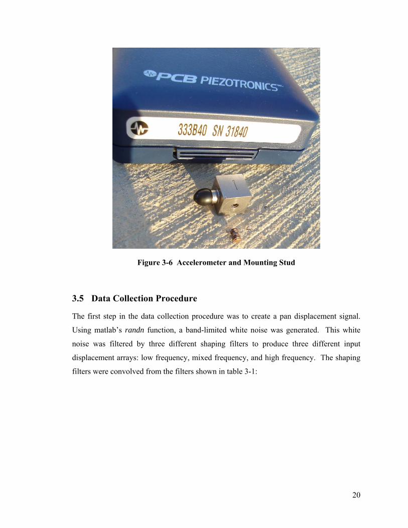
Figure 3-6 Accelerometer and Mounting Stud

3.5 Data Collection Procedure

The first step in the data collection procedure was to create a pan displacement signal.

Using matlab’s randn function, a band-limited white noise was generated. This white

noise was filtered by three different shaping filters to produce three different input

displacement arrays: low frequency, mixed frequency, and high frequency. The shaping

filters were convolved from the filters shown in table 3-1:

20

Table 3-1 Filtering Matrix

Filters Convolved to Form Shaping Filters Input

Displacement 1-pole

1Hz

3-pole

8Hz

4-pole

80Hz

1-pole

20Hz

4-pole

75Hz

Low Frequency

Mixed Frequency

High Frequency

The low frequency displacement input was used in this thesis. This input displacement

was transferred to the MTS controller and used to drive the actuator and quarter-car

suspension. Actuator displacement and sprung and unsprung mass acceleration vs. time

were recorded using the actuator LVDT and accelerometers. For compatibility with the

HHT numerical integrator used for simulation, high frequency noise present in the

actuator displacement signal is filtered using a 4-Pole 50 Hz Butterworth Filter. This

filtering operation was implemented on all the data using Matlab’s filtfilt function to

provide zero phase distortion. Filtering the data in such a way is permissible because

major suspension dynamics occur at much lower frequencies (first mode at ~4 Hz and

second mode at ~28 Hz) and because most of the energy, as seen in spectral plots, is

below 50 Hz.

Measured pan displacement vs. time using the low frequency input displacement is

shown in Figures 3-7 and 3-8. Likewise, Figures 3-9 and 3-10 show the measured sprung

and unsprung mass accelerations vs. time using the low frequency input displacement.

Several observations can be made about the experimentally-measured sprung and

unsprung mass accelerations. First, it is apparent that the sprung mass acceleration has

filtered high frequency acceleration content found in the unsprung mass. Likewise, the

sprung mass acceleration follows the same general pattern as the unsprung mass. Both of

these characteristics are expected byproducts of vehicular suspensions. It is also

expected that the peak sprung mass accelerations are less than the unsprung mass

accelerations. However, because this race car-derived suspension is designed for an

21

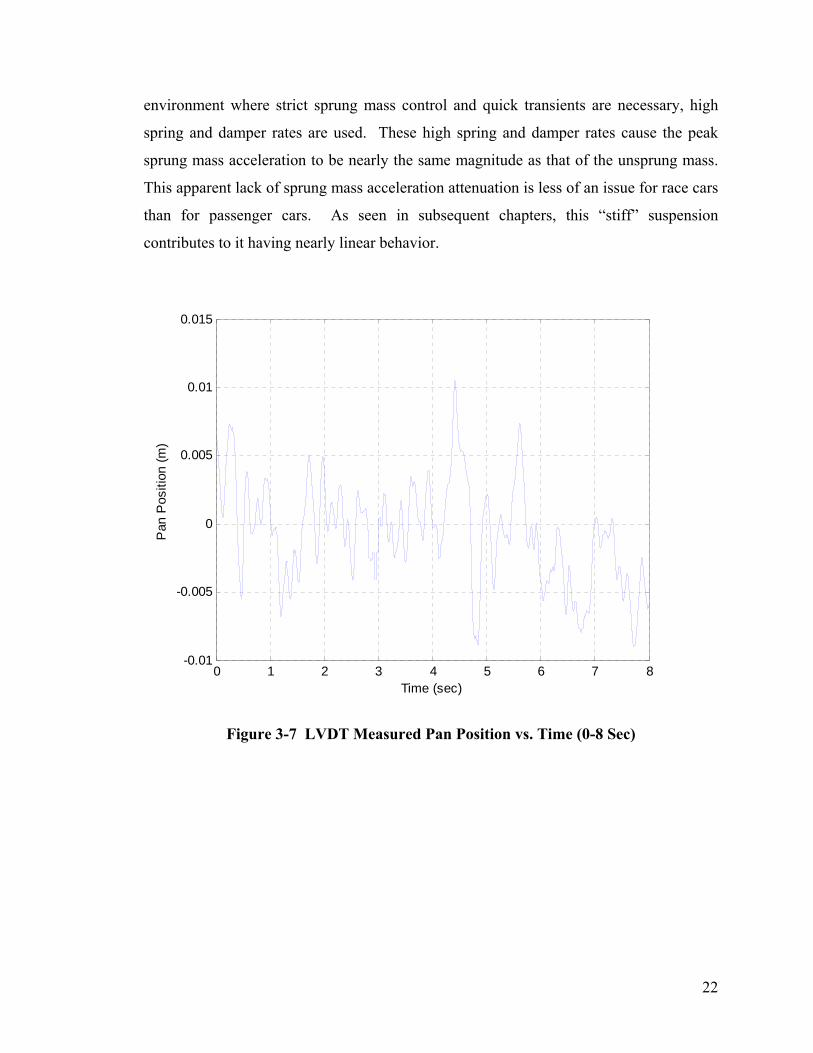
environment where strict sprung mass control and quick transients are necessary, high

spring and damper rates are used. These high spring and damper rates cause the peak

sprung mass acceleration to be nearly the same magnitude as that of the unsprung mass.

This apparent lack of sprung mass acceleration attenuation is less of an issue for race cars

than for passenger cars. As seen in subsequent chapters, this “stiff” suspension

contributes to it having nearly linear behavior.

0 1 2 3 4 5 6 7 8-0.01

-0.005

0

0.005

0.01

0.015

Pan

Pos

ition

(m)

Time (sec)

Figure 3-7 LVDT Measured Pan Position vs. Time (0-8 Sec)

22

5 5.1 5.2 5.3 5.4 5.5 5.6 5.7 5.8 5.9 6-0.01

-0.008

-0.006

-0.004

-0.002

0

0.002

0.004

0.006

0.008

0.01

Pan

Pos

ition

(m)

Time (sec)

Figure 3-8 LVDT Measured Pan Position vs. Time (5-6 Sec)

0 1 2 3 4 5 6 7 8-0.5

0

0.5

a s (g)

0 1 2 3 4 5 6 7 8-0.5

0

0.5

a u (g)

Time (s)

Figure 3-9 Measured Sprung and Unsprung Mass Acceleration vs. Time (0-8 Sec)

23

5 5.1 5.2 5.3 5.4 5.5 5.6 5.7 5.8 5.9 6-0.5

0

0.5

a s (g)

5 5.1 5.2 5.3 5.4 5.5 5.6 5.7 5.8 5.9 6-0.5

0

0.5

a u (g)

Time (s)

Figure 3-10 Measured Sprung and Unsprung Mass Acceleration vs. Time (5-6 Sec)

24

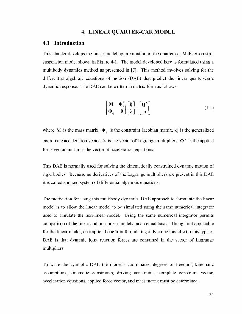
4. LINEAR QUARTER-CAR MODEL

4.1 Introduction

This chapter develops the linear model approximation of the quarter-car McPherson strut

suspension model shown in Figure 4-1. The model developed here is formulated using a

multibody dynamics method as presented in [7]. This method involves solving for the

differential algebraic equations of motion (DAE) that predict the linear quarter-car’s

dynamic response. The DAE can be written in matrix form as follows:

⎡ ⎤ ⎡ ⎤⎡ ⎤⎢ ⎥ ⎢ ⎥⎢ ⎥⎢ ⎥ ⎣ ⎦ ⎣ ⎦⎣ ⎦

T Aq

q

M Φ q Q=

Φ 0 λ α&&

(4.1)

where is the mass matrix, is the constraint Jacobian matrix, q&& is the generalized

coordinate acceleration vector, λ is the vector of Lagrange multipliers, is the applied

force vector, and is the vector of acceleration equations.

M qΦ

AQ

α

This DAE is normally used for solving the kinematically constrained dynamic motion of

rigid bodies. Because no derivatives of the Lagrange multipliers are present in this DAE

it is called a mixed system of differential algebraic equations.

The motivation for using this multibody dynamics DAE approach to formulate the linear

model is to allow the linear model to be simulated using the same numerical integrator

used to simulate the non-linear model. Using the same numerical integrator permits

comparison of the linear and non-linear models on an equal basis. Though not applicable

for the linear model, an implicit benefit in formulating a dynamic model with this type of

DAE is that dynamic joint reaction forces are contained in the vector of Lagrange

multipliers.

To write the symbolic DAE the model’s coordinates, degrees of freedom, kinematic

assumptions, kinematic constraints, driving constraints, complete constraint vector,

acceleration equations, applied force vector, and mass matrix must be determined.

25

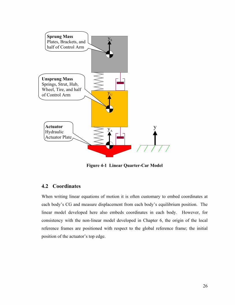
Sprung Mass Plates, Brackets, and half of Control Arm

Unsprung Mass Springs, Strut, Hub, Wheel, Tire, and half of Control Arm

Actuator Hydraulic Actuator Plate

Sy

Uy

yAy

Figure 4-1 Linear Quarter-Car Model

4.2 Coordinates

When writing linear equations of motion it is often customary to embed coordinates at

each body’s CG and measure displacement from each body’s equilibrium position. The

linear model developed here also embeds coordinates in each body. However, for

consistency with the non-linear model developed in Chapter 6, the origin of the local

reference frames are positioned with respect to the global reference frame; the initial

position of the actuator’s top edge.

26

The linear model consists of sprung, unsprung, and actuator bodies. Reference frames

are embedded at the CG of the sprung and unsprung masses and at the top edge of the

actuator. The global Y-position of each body is measured from its respective reference

frame to the global Y reference frame. The vector of coordinates that fully define the

global position of these bodies is:

[ ]TS U Ay y y=q (4.2)

Subscripts S, U, and A are abbreviations for sprung mass, unsprung mass, and actuator.

4.3 Degrees of Freedom

For linear systems, the degrees of freedom (DOF) present is the number of masses minus

the number of driving constraints. For example, a three-mass system with one driven

mass, such as the one shown in Figure 4-1, would have two DOF. Determination of the

DOF in a multibody dynamics model is extended to include the constraints that joints

place on the model.

The DOF present in any multibody dynamics model is the number of coordinates minus

the sum of independent kinematic and driving constraint equations. Normally kinematic

constraint equations are written based on how each joint constrains the motion of

connected bodies. However, the linear model has no joints and therefore does not have

kinematic constraint equations. Chapter 6 presents examples of how kinematic constraint

equations are developed. The driven hydraulic actuator creates one driving constraint

equation. In sum, there is one independent kinematic and driving constraint equation. In

consideration of its three coordinates, the linear model has two DOF. One DOF is

associated with the displacement of the sprung mass and the other with the unsprung

mass.

27

4.4 Kinematic Assumptions and Constraints

The major assumption made with the linear model is that the motion of the bodies in the

system can be approximated as linear. In actuality the unsprung mass, and hence the strut

and control arm angles, change during suspension motion. Because the linear model does

not account for this angular motion the vertical motion of the sprung mass and the strut

force are approximate.

Also, because the linear model has no joints it does not have kinematic constraint

equations. However, implicit kinematic constraints arise by specifying only vertical

coordinates. By omitting horizontal and rotational coordinates there is no need to

introduce translational joints to constrain them.

4.5 Driving Constraint

Driving constraints prescribe the motion of driven bodies. The servo-hydraulic actuator

is the driven body in this system and provides one driving constraint. In general, the

driven DOF is a function of time and the model’s coordinates: . For

this model the actuator position is a function only of time and can be written as the time

history of its position:

( )A S, ,y f t y y= U

( )Ay f t= . Thus the driving constraint is:

( )DA 0y f t⎡ ⎤Φ = − =⎣ ⎦ (4.3)

4.6 Complete Constraint Vector

The complete constraint vector is a combination of the kinematic and driving constraints:

( )K

DAD 0y f t

⎡ ⎤⎡ ⎤ ⎡ ⎤= = Φ = − =⎢ ⎥ ⎣ ⎦⎣ ⎦

⎣ ⎦

ΦΦ

Φ (4.4)

28

where is the kinematic constraint vector and is the driving constraint. In this

case

KΦ

[

DΦ

]K =Φ 0 .

From this complete constraint vector, the Jacobian of the constraints, a matrix that plays a

pivotal role in formulating the DAE, can be obtained [7]. Mathematically, the Jacobian is

the partial derivative of the complete constraint vector with respect to each coordinate.

Each row of the Jacobian is associated with a constraint equation. Each column of the

Jacobian is associated with a coordinate. For example, an element in the third row and

second column of the Jacobian is the derivative of the third constraint equation with

respect to the second coordinate. In this case, since there is only one constraint equation,

the Jacobian has only one row. The first column is the derivative of the constraint with

respect to Sy , the second column is the derivative with respect to Uy , and the third

column is the derivative with respect to Ay . Using ‘i’ and ‘j’ as the row and column

indices, the linear model’s Jacobian is:

( )( ) ( )( ) ( )( ) [ ]A A Ai

qj S U A1 3

Φ 0 0 1y f t y f t y f t

q y y y×

⎡ ⎤⎡ ⎤ ∂ − ∂ − ∂ −∂∂= = = =⎢ ⎥⎢ ⎥∂ ∂ ∂ ∂ ∂⎢ ⎥ ⎢ ⎥⎣ ⎦ ⎣ ⎦

ΦΦq

(4.5)

To assure that the system is not over constrained the rows of the Jacobian must be

linearly independent. This Jacobian has full-row rank, and therefore the constraint

equation is independent; that is, the system is not over-constrained.

4.7 Acceleration Equations

The acceleration equation can be obtained [7] as:

( )q q qtq− − −α = Φ q = Φ q q 2Φ q Φ&& & & & tt (4.6)

The terms that make up the acceleration equation are as follows:

29

2

tt 21

Φi

nht×

⎡ ⎤∂= ⎢ ⎥∂⎣ ⎦

Φ (4.7)

2

qtΦi

j nh ncq t

×

⎡ ⎤∂= ⎢ ⎥

∂ ∂⎢ ⎥⎣ ⎦Φ (4.8)

( )q q1

Φ qnc

ik

kj k nh ncq q= ×

⎡ ⎤⎛ ⎞∂∂= ⎢ ⎜ ⎟∂ ∂⎢ ⎥⎝ ⎠⎣ ⎦

∑Φ q& ⎥& (4.9)

where ‘nc’ denotes the number of coordinates and ‘nh’ denotes the number of holonomic

constraint equations. Holonomic constraint equations are those that can be expressed in

terms of generalized coordinates. Nonholonomic constraint equations are more general

in that they can be expressed as inequalities and may be functions of time or velocity.

It is foreseeable that a variety of driving inputs will be used to drive the quarter-car’s

actuator. Therefore the function ( )f t defining this input is kept general. Adhering to

this idea, the term is: ttΦ

( )2

tt 2

f tt

⎡ ⎤∂= ⎢ ⎥∂⎣ ⎦

Φ (4.10)

Because has no explicitly time dependent terms, is zero. The third acceleration

term is solved piecewise below:

qΦ qtΦ

[ ] [S

q U

A

0 0 1y

]Ay yy

⎡ ⎤⎢ ⎥= ⎢ ⎥⎢ ⎥⎣ ⎦

Φ q&

& & &

&

= (4.11)

( ) ( ) [ ]q A qq0 0 0y= =Φ q& & (4.12)

30

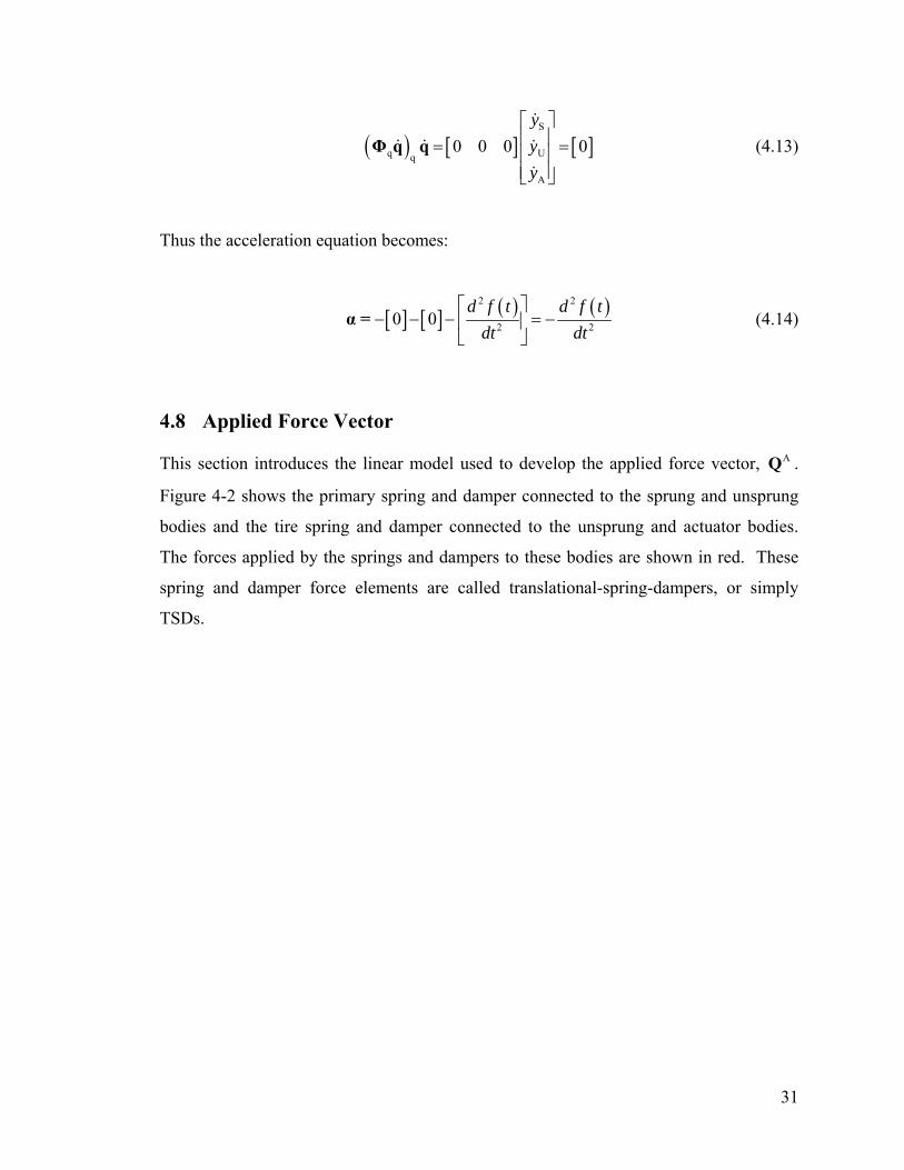
(4.13) ( ) [ ]S

q q

A

0 0 0 0yyy

⎡ ⎤⎢ ⎥= ⎢ ⎥⎢ ⎥⎣ ⎦

Φ q q&

& & &

&

[ ]U =

Thus the acceleration equation becomes:

[ ] [ ] ( ) ( )2 2

20 0d f t d f t

dt dt⎡ ⎤

− − − = −⎢ ⎥⎣ ⎦

α = 2 (4.14)

4.8 Applied Force Vector

This section introduces the linear model used to develop the applied force vector, .

Figure 4-2 shows the primary spring and damper connected to the sprung and unsprung

bodies and the tire spring and damper connected to the unsprung and actuator bodies.

The forces applied by the springs and dampers to these bodies are shown in red. These

spring and damper force elements are called translational-spring-dampers, or simply

TSDs.

AQ

31

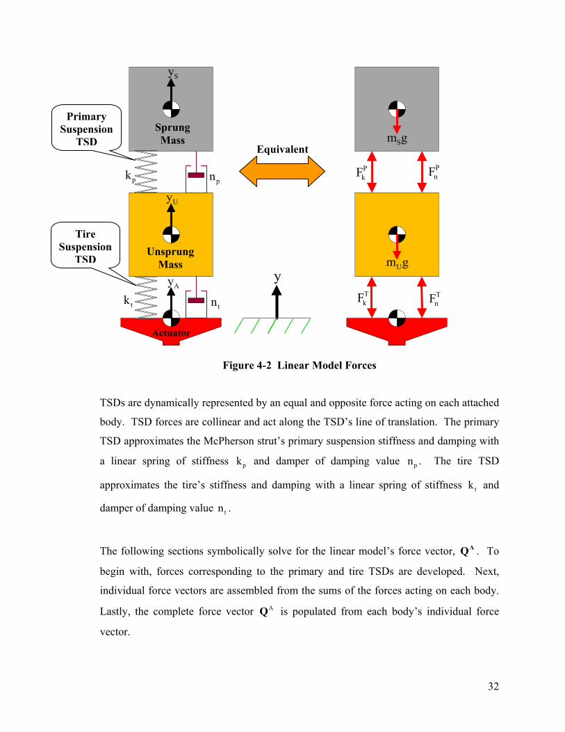
Figure 4-2 Linear Model Forces

TSDs are dynamically represented by an equal and opposite force acting on each attached

body. TSD forces are collinear and act along the TSD’s line of translation. The primary

TSD approximates the McPherson strut’s primary suspension stiffness and damping with

a linear spring of stiffness pk and damper of damping value pn . The tire TSD

approximates the tire’s stiffness and damping with a linear spring of stiffness and

damper of damping value .

tk

tn

The following sections symbolically solve for the linear model’s force vector, . To

begin with, forces corresponding to the primary and tire TSDs are developed. Next,

individual force vectors are assembled from the sums of the forces acting on each body.

Lastly, the complete force vector is populated from each body’s individual force

vector.

AQ

AQ

Primary Suspension

TSD

tntk

pnpk

Sy

Uy

Ay

PnF

Sprung Mass Sm g

Equivalent PkF

Tire Suspension

TSDUnsprung

Mass

Actuator

Um gy

TkF T

nF

32

4.8.1 Primary TSD

This section develops the force created by the primary TSD. The primary TSD, shown in

Figure 4-3, produces a force along the global Y-direction in proportion to its

compression and compression velocity .

PF

USdΔ USdΔ&

PF

DUSd ypk

pn

PF

Figure 4-3 Linear Model Primary TSD

To specify the primary TSD compression, its initial and displaced length must be

determined. The initial length, d , is its length without any load on it, or free length.

The displaced length, , is the global sprung mass Y-position minus the unsprung

mass Y-position. Thus, the primary TSD compression is:

IUS

DUSd

(4.15)

( )I D

I

US

US US US

US US S U

d Initial length Displaced lengthd d d

d d y y

Δ = −Δ = −

Δ = − −

33

Positive spring forces are applied outward from the TSD’s center towards the sprung and

unsprung mass when the spring is compressed.

The first time derivative of primary TSD compression is the primary TSD compression

velocity:

US S Ud y yΔ = − +& & & (4.16)

Positive damper forces are applied outward from the TSD’s center towards the sprung

and unsprung mass when the damper is compressing. The red vectors in Figure 4-3 show

the positive primary TSD force direction. The outward primary TSD force is the sum of

its spring and damper forces:

(4.17)

P

P P Pk n

Pp US p US

F Primary Spring Force Primary Damper ForceF F F

F k d n d

= +

= +

= Δ + Δ&

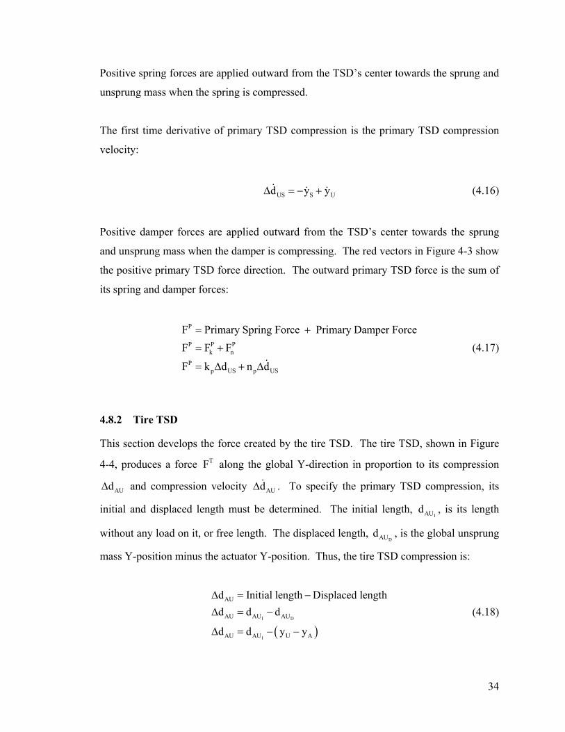
4.8.2 Tire TSD

This section develops the force created by the tire TSD. The tire TSD, shown in Figure

4-4, produces a force along the global Y-direction in proportion to its compression

and compression velocity . To specify the primary TSD compression, its

initial and displaced length must be determined. The initial length, , is its length

without any load on it, or free length. The displaced length, , is the global unsprung

mass Y-position minus the actuator Y-position. Thus, the tire TSD compression is:

TF

AUdΔ AUdΔ&

IAUd

DAUd

(4.18)

( )I D

I

AU

AU AU AU

AU AU U A

d Initial length Displaced lengthd d d

d d y y

Δ = −Δ = −

Δ = − −

34

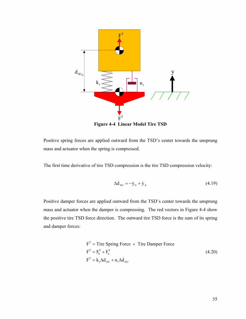
tn

Figure 4-4 Linear Model Tire TSD

tkDAUd

TF

TF

y

Positive spring forces are applied outward from the TSD’s center towards the unsprung

mass and actuator when the spring is compressed.

The first time derivative of tire TSD compression is the tire TSD compression velocity:

AU U Ad y yΔ = − +& & & (4.19)

Positive damper forces are applied outward from the TSD’s center towards the unsprung

mass and actuator when the damper is compressing. The red vectors in Figure 4-4 show

the positive tire TSD force direction. The outward tire TSD force is the sum of its spring

and damper forces:

(4.20)

T

T T Tk n

Tt AU t AU

F Tire Spring Force Tire Damper ForceF F F

F k d n d

= +

= +

= Δ + Δ&

35

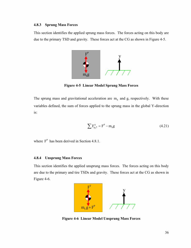
4.8.3 Sprung Mass Forces

This section identifies the applied sprung mass forces. The forces acting on this body are

due to the primary TSD and gravity. These forces act at the CG as shown in Figure 4-5.

PF y

Sm g

Figure 4-5 Linear Model Sprung Mass Forces

The sprung mass and gravitational acceleration are and g, respectively. With these

variables defined, the sum of forces applied to the sprung mass in the global Y-direction

is:

Sm

A PSSyF F m↑ = − g∑ (4.21)

where has been derived in Section 4.8.1. PF

4.8.4 Unsprung Mass Forces

This section identifies the applied unsprung mass forces. The forces acting on this body

are due to the primary and tire TSDs and gravity. These forces act at the CG as shown in

Figure 4-6.

TF y

PUm g F+

Figure 4-6 Linear Model Unsprung Mass Forces

36

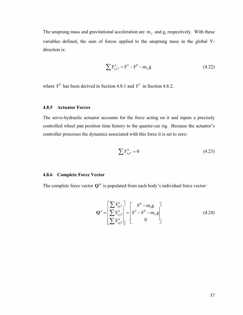
The unsprung mass and gravitational acceleration are and g, respectively. With these

variables defined, the sum of forces applied to the unsprung mass in the global Y-

direction is:

Um

A T PUUyF F F m↑ = − − g∑ (4.22)

where has been derived in Section 4.8.1 and in Section 4.8.2. PF TF

4.8.5 Actuator Forces

The servo-hydraulic actuator accounts for the force acting on it and inputs a precisely

controlled wheel pan position time history to the quarter-car rig. Because the actuator’s

controller processes the dynamics associated with this force it is set to zero:

AAyF ↑ 0=∑ (4.23)

4.8.6 Complete Force Vector

The complete force vector is populated from each body’s individual force vector: AQ

A PSy S

A A T PUUy

AAy

F F m gF F F m

0F

↑

↑

↑

⎡ ⎤

g⎡ ⎤−

⎢ ⎥ ⎢ ⎥= = − −⎢ ⎥ ⎢ ⎥⎢ ⎥ ⎢ ⎥⎣ ⎦⎢ ⎥⎣ ⎦

∑∑∑

Q (4.24)

37

4.9 Mass Matrix

The mass matrix for the linear model has the form:

S

U

A

m 0 00 m 00 0 m

⎡ ⎤⎢ ⎥= ⎢ ⎥⎢ ⎥⎣ ⎦

M (4.25)

where , , and are the sprung, unsprung, and actuator masses. The sprung

mass includes mass from the sprung mass plate, adapter plate, strut tower, and ballast

weights. The unsprung mass includes mass from the springs, damper, upright, brake

disk, wheel, and tire. Tie-rod and control arm masses are split evenly between the sprung

and unsprung masses. The actuator mass is considered negligible in this study and is

approximated as zero. For completeness and for easy adjustment of the model in the

future, the dynamic equation associated with is kept in the system of equations.

Sm Um Am

Am

4.10 McPherson Strut Linear DAE

With all the components of the DAE determined, it can be assembled. The DAE used to

simulate the linear quarter-car’s dynamic response is:

( )

PS

SS T PU

UU

AA 2

1 2

F m gm 0 0 0F F m g0 m 0 0

00 0 m 10 0 1 0

yyy

d f tdt

λ

⎡ ⎤ ⎡ ⎤⎡ ⎤⎢ ⎥ ⎢ ⎥⎢ ⎥⎢ ⎥ ⎣ ⎦ ⎣ ⎦⎣ ⎦

⎡ ⎤−⎡ ⎤⎡ ⎤ ⎢ ⎥− −⎢ ⎥⎢ ⎥ ⎢ ⎥⎢ ⎥⎢ ⎥ ⎢ ⎥=⎢ ⎥⎢ ⎥ ⎢ ⎥⎢ ⎥⎢ ⎥ ⎢ ⎥

−⎣ ⎦ ⎣ ⎦ ⎢ ⎥⎣ ⎦

T Aq

q

M Φ q Q=

Φ 0 λ α&&

&&

&&

&&

(4.26)

38

5. LINEAR QUARTER-CAR MODEL SYSTEM IDENTIFICATION

5.1 Introduction

This chapter presents the background and results of the system identification of the linear

quarter-car McPherson strut suspension model developed in Chapter 4. The purpose of

this system identification is to determine model parameters that best facilitate the linear

model’s prediction of the experimental sprung and unsprung mass accelerations. Using

these parameters with the linear model will create an optimal linear model that can be

used for dynamic response prediction and control algorithm design.

5.2 Hilber-Hughes-Taylor DAE Integrator

A Hilber-Hughes-Taylor (HHT) method integrator was used to solve the system of

DAEs. In addition to being capable of solving DAE equations this method is attractive

because of its intrinsic stability. Negrut [13] mentions that “models that are mechanically

stiff [can land other integrators] outside the stability region [but this] is a non-issue with

the HHT method, which is a fixed low-order method with good stability properties in the

whole left plane.” The basic fixed time step HHT algorithm employed in this study is as

follows:

1) Set initial conditions and parameters

2) Calculate initial acceleration

3) Enter main-loop

a. Calculate values that remain constant during each time step

i. Enter sub-loop

1. Calculate force and kinematic residuals

2. From residuals solve for delta vector

3. Add delta vector to state vector

ii. End sub-loop when residuals and delta are less than epsilon

b. Record state vector

4) End main-loop when all time steps have been solved

39

The state vector refers to the vector of positions, velocities, accelerations, and Lagrange

multipliers. Residuals are calculated based on the current state vector. The sub-loop uses

multiple function evaluations to predict the state vector that minimizes the residuals, and

thus this method is closer to a predictor-corrector method than a Euler method. The sub-

loop terminates when the norm of the residuals and the norm of the delta vector are less

than epsilon. In this way the HHT algorithm provides a user-specified error tolerance.

For this study, epsilon was chosen to be 410ε −= because this value allowed timely

simulation and because the simulation was not significantly more accurate with a lower

epsilon.

Another value that must be specified with this method is alpha. From an implementation

standpoint, a lower alpha value corresponds to a shorter simulation transient period.

Alpha was chosen to be the minimum allowable for this method ( 1 3α = − ) to shorten

the initial simulation transient. With these constants specified, the HHT integrator was

used to solve the DAE system and served as the basic algorithm to which system

identification was applied.

5.3 System Identification

System identification was performed by minimizing the acceleration error function:

( ) ( ) ( )( ) ( ) ( )

( ) ( )

( ) ( )

S S

U U

S S S1

U U U1

S U

i Exp_a i Sim_a i

i Exp_a i Sim_a i

f i i

f i i

f = f f

n

n

e

e

e e

e e

= −

= −

= ⋅

= ⋅

+

∑

∑

S

U

(5.1)

where and are the experimental sprung and unsprung mass acceleration

arrays, and

SExp_a

SSim_a

UExp_a

( )i ( )U_a iSim are the simulated sprung and unsprung mass

40

acceleration arrays, and are the sprung and unsprung mass acceleration error

arrays, and are the sum-of-squared sprung and unsprung mass acceleration error

scalars, and is the total acceleration error function. In finding a minimum to this error

function, also called the cost function, the system identification process finds optimal

parameter values. In this case, optimal parameters are defined as parameters that

minimize the difference between the simulated and experimental sprung and unsprung

mass accelerations. Using these optimized parameters with the linear quarter-car model

allows it to best predict the sprung and unsprung mass accelerations.

Se Ue

Sf Uf

f

5.4 Procedure

This section describes the method used to perform system identification. To perform

system identification, one selects the period over which the cost function is evaluated, the

parameters to be optimized, and the upper and lower parameter bounds.

The comparison period used to generate the cost function was 3-8 seconds. This interval

was chosen because it allows sufficient time for the simulation to pass its transient, yet it

is short enough to ensure that the system identification time was not excessive.

The optimization parameters selected for linear model system identification include the

sprung mass, unsprung mass, the stiffness values, and damping values. Initial values for

these parameters were gathered by direct measurement, calculation, or estimation. Figure

5-1 shows the initial parameter estimates that comprise the non-optimized parameters.

Figure 5-2 shows the initial positions and velocities.

The choice of parameter bounds directly affects the quantity of separate system

identification runs needed to converge to optimal parameters. If the system identification

process arrives at a parameter equal to that parameter’s bound, it may be the optimal

parameter or it may be the best parameter available based on the bound limitation set. In

order to find out which is the case, this parameter’s bound must be expanded and

subsequent system identification performed. Subsequent system identification uses the

41

optimal parameters solved for in the previous system identification. In the interest of

avoiding the system identification process solving for optimal parameters at its bounds,

and thus having to perform subsequent system identification, the initial bounds are

broadly spaced. If subsequent system identification is needed, the bounds are less

broadly spaced. Further system identification is not run if none of the optimized

parameters are at a bound or if extending the bound has minimal effect on the model’s

performance.

42

( )( )( )( )

( )( )( )( )

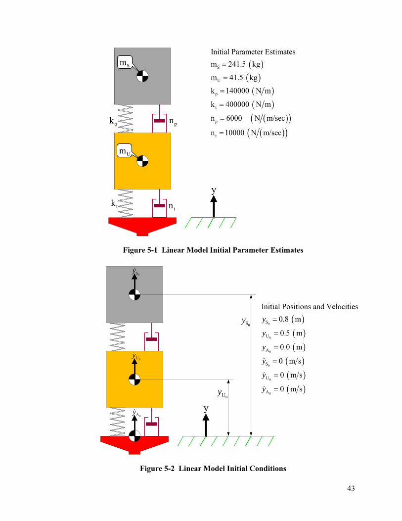
S

U

p

t

p

t

Initial Parameter Estimatesm 241.5 kg

m 41.5 kg

k 140000 N m

k 400000 N m

n 6000 N m/sec

n 10000 N m/sec

=

=

=

=

=

=

Sm

Um

tktn

Figure 5-1 Linear Model Initial Parameter Estimates

pk pn

y

0Sy&

( )( )( )

( )( )( )

0

0

0

0

0

0

S

U

A

S

U

A

Initial Positions and Velocities0.8 m

0.5 m

0.0 m

0 m s

0 m s

0 m s

y

y

y

y

y

y

=

=

=

=

=

=

&

&

&

0Sy

0Uy&

0Uy

y0Ay&

Figure 5-2 Linear Model Initial Conditions

43

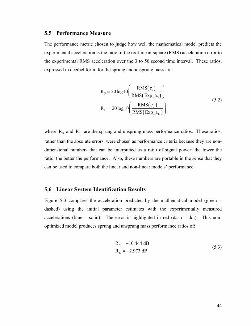
5.5 Performance Measure

The performance metric chosen to judge how well the mathematical model predicts the

experimental acceleration is the ratio of the root-mean-square (RMS) acceleration error to

the experimental RMS acceleration over the 3 to 50 second time interval. These ratios,

expressed in decibel form, for the sprung and unsprung mass are:

( )( )

( )( )

SS

S

UU

U

RMSR 20log10

RMS Exp_a

RMSR 20log10

RMS Exp_a

e

e

⎛ ⎞= ⎜ ⎟⎜ ⎟

⎝⎛ ⎞

= ⎜ ⎟⎜ ⎟⎝ ⎠

⎠ (5.2)

where and are the sprung and unsprung mass performance ratios. These ratios,

rather than the absolute errors, were chosen as performance criteria because they are non-

dimensional numbers that can be interpreted as a ratio of signal power: the lower the

ratio, the better the performance. Also, these numbers are portable in the sense that they

can be used to compare both the linear and non-linear models’ performance.

SR UR

5.6 Linear System Identification Results

Figure 5-3 compares the acceleration predicted by the mathematical model (green –

dashed) using the initial parameter estimates with the experimentally measured

accelerations (blue – solid). The error is highlighted in red (dash – dot). This non-

optimized model produces sprung and unsprung mass performance ratios of:

S

U

R 10.444 dB R 2.973 dB

= −= −

(5.3)

44

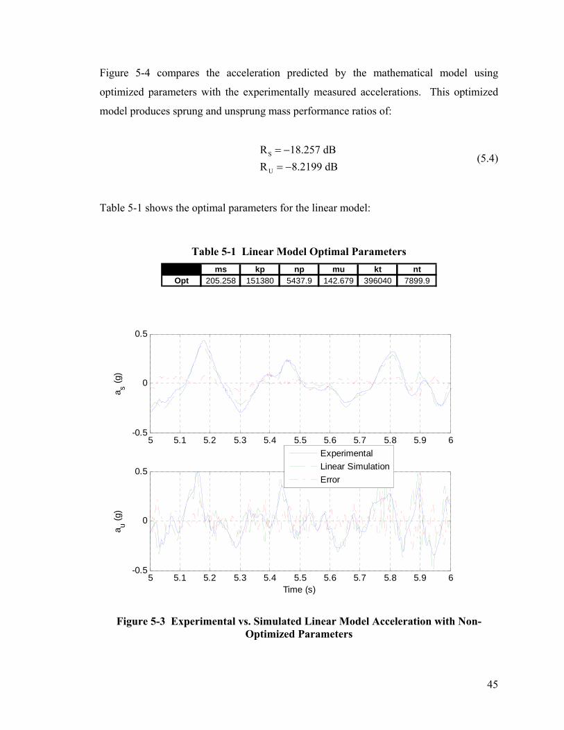
Figure 5-4 compares the acceleration predicted by the mathematical model using

optimized parameters with the experimentally measured accelerations. This optimized

model produces sprung and unsprung mass performance ratios of:

S

U

R 18.257 dBR 8.2199 dB

= −= −

(5.4)

Table 5-1 shows the optimal parameters for the linear model:

Table 5-1 Linear Model Optimal Parameters ms kp np mu kt nt

Opt 205.258 151380 5437.9 142.679 396040 7899.9

5 5.1 5.2 5.3 5.4 5.5 5.6 5.7 5.8 5.9 6-0.5

0

0.5

a s (g)

5 5.1 5.2 5.3 5.4 5.5 5.6 5.7 5.8 5.9 6-0.5

0

0.5

a u (g)

Time (s)

ExperimentalLinear SimulationError

Figure 5-3 Experimental vs. Simulated Linear Model Acceleration with Non-Optimized Parameters

45

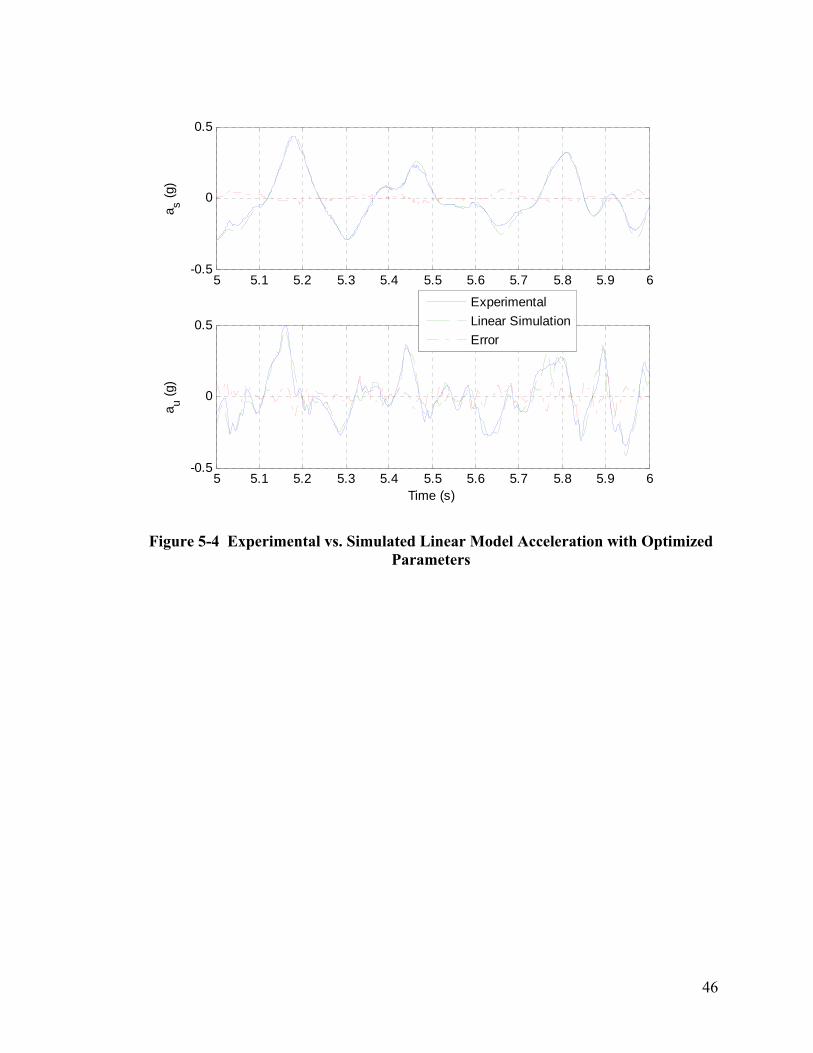
5 5.1 5.2 5.3 5.4 5.5 5.6 5.7 5.8 5.9 6-0.5

0

0.5

a s (g)

5 5.1 5.2 5.3 5.4 5.5 5.6 5.7 5.8 5.9 6-0.5

0

0.5

a u (g)

Time (s)

ExperimentalLinear SimulationError

Figure 5-4 Experimental vs. Simulated Linear Model Acceleration with Optimized Parameters

46

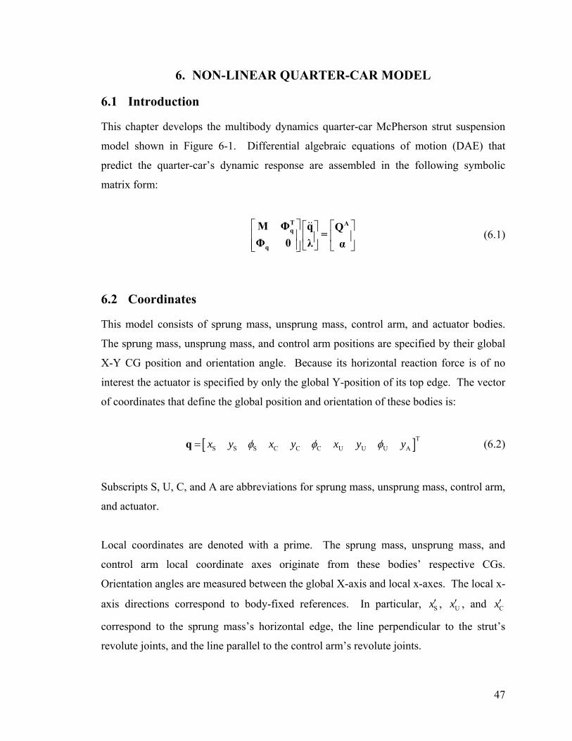
6. NON-LINEAR QUARTER-CAR MODEL

6.1 Introduction

This chapter develops the multibody dynamics quarter-car McPherson strut suspension

model shown in Figure 6-1. Differential algebraic equations of motion (DAE) that

predict the quarter-car’s dynamic response are assembled in the following symbolic

matrix form:

⎡ ⎤ ⎡ ⎤⎡ ⎤⎢ ⎥ ⎢ ⎥⎢ ⎥⎢ ⎥ ⎣ ⎦ ⎣ ⎦⎣ ⎦

T Aq

q

M Φ q Q=

Φ 0 λ α&&

(6.1)

6.2 Coordinates

This model consists of sprung mass, unsprung mass, control arm, and actuator bodies.

The sprung mass, unsprung mass, and control arm positions are specified by their global

X-Y CG position and orientation angle. Because its horizontal reaction force is of no

interest the actuator is specified by only the global Y-position of its top edge. The vector

of coordinates that define the global position and orientation of these bodies is:

[ ]TS S S C C C U U U Ax y x y x y yφ φ φ=q (6.2)

Subscripts S, U, C, and A are abbreviations for sprung mass, unsprung mass, control arm,

and actuator.

Local coordinates are denoted with a prime. The sprung mass, unsprung mass, and

control arm local coordinate axes originate from these bodies’ respective CGs.

Orientation angles are measured between the global X-axis and local x-axes. The local x-

axis directions correspond to body-fixed references. In particular, Sx′ , Ux′ , and Cx′

correspond to the sprung mass’s horizontal edge, the line perpendicular to the strut’s

revolute joints, and the line parallel to the control arm’s revolute joints.

47

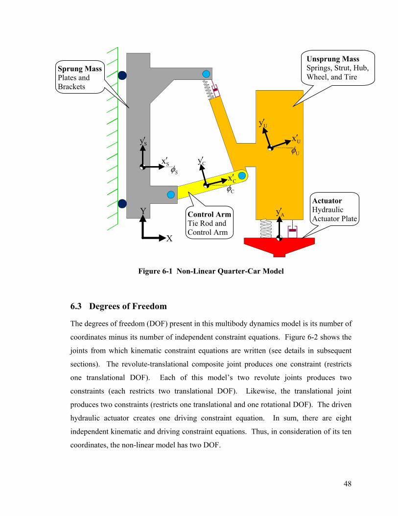
Unsprung Mass Springs, Strut, Hub, Wheel, and Tire

Sprung Mass Plates and Brackets

Uy′

Ux′Sy′

S

Uφ

Figure 6-1 Non-Linear Quarter-Car Model

6.3 Degrees of Freedom

The degrees of freedom (DOF) present in this multibody dynamics model is its number of

coordinates minus its number of independent constraint equations. Figure 6-2 shows the

joints from which kinematic constraint equations are written (see details in subsequent

sections). The revolute-translational composite joint produces one constraint (restricts

one translational DOF). Each of this model’s two revolute joints produces two

constraints (each restricts two translational DOF). Likewise, the translational joint

produces two constraints (restricts one translational and one rotational DOF). The driven

hydraulic actuator creates one driving constraint equation. In sum, there are eight

independent kinematic and driving constraint equations. Thus, in consideration of its ten

coordinates, the non-linear model has two DOF.

Control ArmTie Rod and Control Arm

Actuator Hydraulic Actuator Plate

φCy′

Cφ

Ay′

X

Y

Sx′

Cx′

48

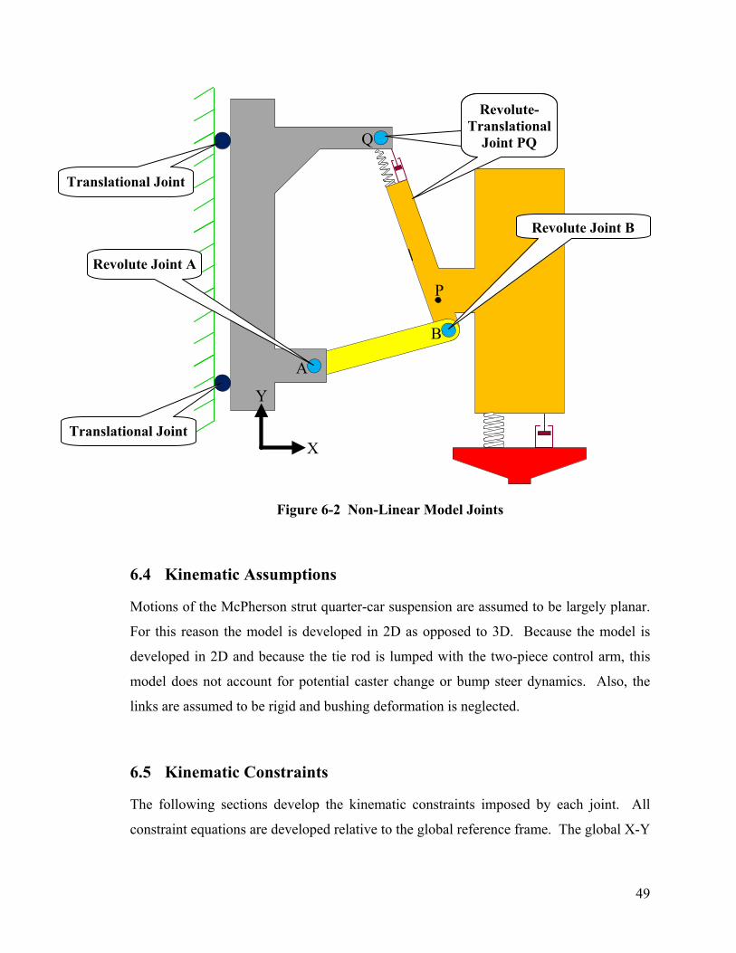
Revolute-

Translational

Revolute-Translational

Joint PQ

Figure 6-2 Non-Linear Model Joints

6.4 Kinematic Assumptions

Motions of the McPherson strut quarter-car suspension are assumed to be largely planar.

For this reason the model is developed in 2D as opposed to 3D. Because the model is

developed in 2D and because the tie rod is lumped with the two-piece control arm, this

model does not account for potential caster change or bump steer dynamics. Also, the

links are assumed to be rigid and bushing deformation is neglected.

6.5 Kinematic Constraints

The following sections develop the kinematic constraints imposed by each joint. All

constraint equations are developed relative to the global reference frame. The global X-Y

Revolute Joint A

X

Y

A

B

Q

Translational Joint

Translational Joint

Revolute Joint B

P

49

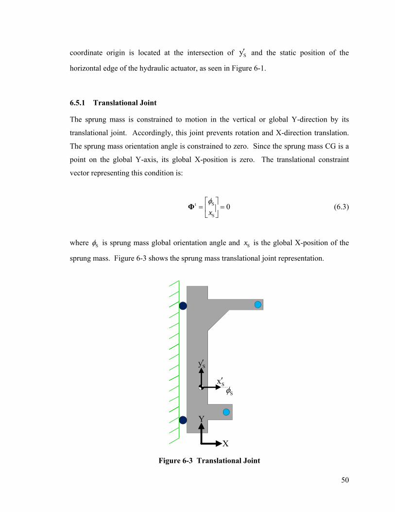
coordinate origin is located at the intersection of Sy′ and the static position of the

horizontal edge of the hydraulic actuator, as seen in Figure 6-1.

6.5.1 Translational Joint

The sprung mass is constrained to motion in the vertical or global Y-direction by its

translational joint. Accordingly, this joint prevents rotation and X-direction translation.

The sprung mass orientation angle is constrained to zero. Since the sprung mass CG is a

point on the global Y-axis, its global X-position is zero. The translational constraint

vector representing this condition is:

St

S

0xφ⎡ ⎤

= =⎢ ⎥⎣ ⎦

Φ (6.3)

where Sφ is sprung mass global orientation angle and Sx is the global X-position of the

sprung mass. Figure 6-3 shows the sprung mass translational joint representation.

Sy′

Figure 6-3 Translational Joint

S′xSφ

X

Y

50

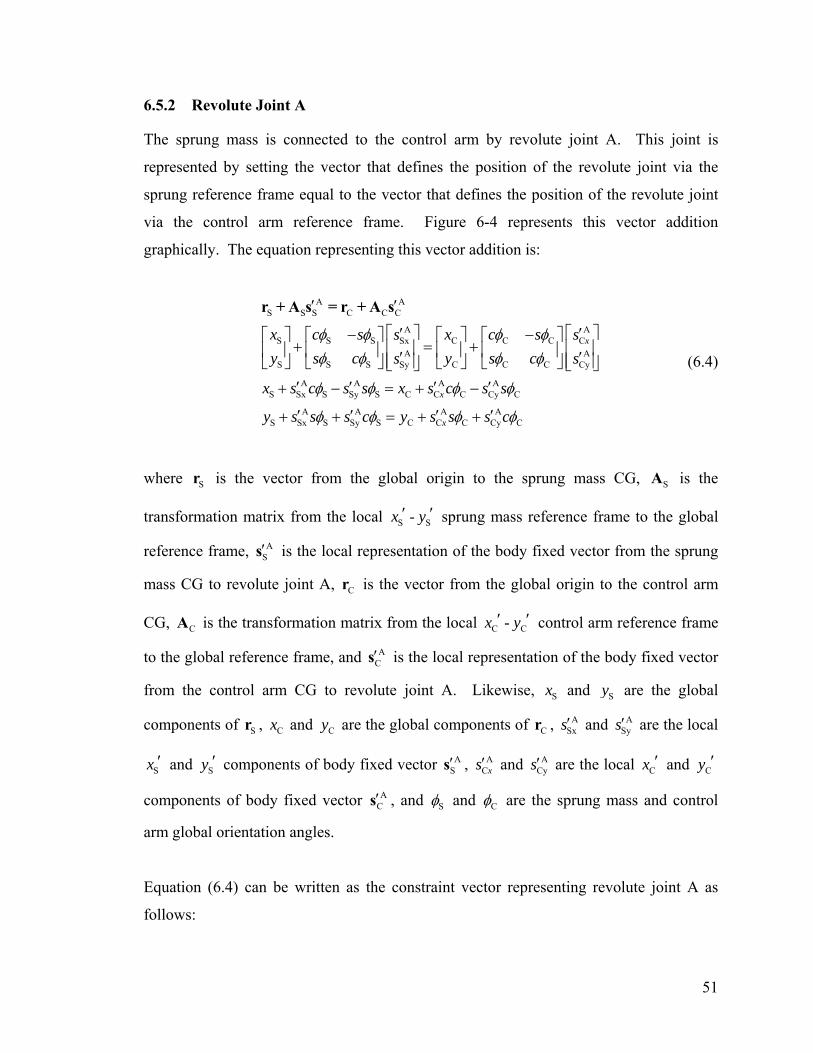
6.5.2 Revolute Joint A

The sprung mass is connected to the control arm by revolute joint A. This joint is

represented by setting the vector that defines the position of the revolute joint via the

sprung reference frame equal to the vector that defines the position of the revolute joint

via the control arm reference frame. Figure 6-4 represents this vector addition

graphically. The equation representing this vector addition is:

A AS S S C C C

A AS S S C C CSx C

AS S S C C CSy Cy

A A A AS Sx S Sy S C C C Cy C

A A A AS Sx S Sy S C C C Cy C

Ax

x

x

x c s x c ss sy s c y s cs

x s c s s x s c s s

y s s s c y s s s c

φ φ φ φφ φ φ φ

φ φ φ φ

φ φ φ φ

′ ′

s⎡ ′ ⎤ ⎡ ′ ⎤− −⎡ ⎤ ⎡ ⎤ ⎡ ⎤ ⎡ ⎤

+ = +⎢ ⎥ ⎢⎢ ⎥ ⎢ ⎥ ⎢ ⎥ ⎢ ⎥ ⎥′ ′⎢ ⎥⎣ ⎦ ⎣ ⎦ ⎣ ⎦ ⎣ ⎦ ⎢ ⎥⎣ ⎦′ ′ ′ ′+ − = + −

′ ′ ′ ′+ + = + +

r + A s = r + A s

⎣ ⎦ (6.4)

where is the vector from the global origin to the sprung mass CG, is the

transformation matrix from the local

Sr SA

Sx ′ - Sy ′ sprung mass reference frame to the global

reference frame, is the local representation of the body fixed vector from the sprung

mass CG to revolute joint A, is the vector from the global origin to the control arm

CG, is the transformation matrix from the local

AS′s

Cr

CA Cx ′ - Cy ′ control arm reference frame

to the global reference frame, and AC′s is the local representation of the body fixed vector

from the control arm CG to revolute joint A. Likewise, Sx and Sy are the global

components of r , S Cx and Cy are the global components of r , CA

Sxs′ and are the local ASy′s

Sx ′ and Sy ′ components of body fixed vector AS′s , A

Cxs′ and ACys′ are the local Cx ′ and Cy ′

components of body fixed vector AC′s , and Sφ and Cφ are the sprung mass and control

arm global orientation angles.

Equation (6.4) can be written as the constraint vector representing revolute joint A as

follows:

51

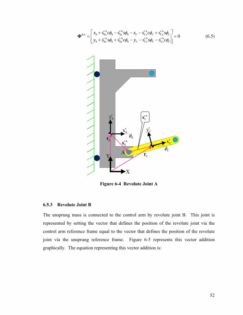
(6.5) A A A A

S Sx S Sy S C C C Cy CRAA A A A

S Sx S Sy S C C C Cy C

0x

x

x s c s s x s c s sy s s s c y s s s c


⎡ ′ ′ ′ ′ ⎤+ − − − += =⎢ ⎥′ ′ ′ ′+ + − − −⎢ ⎥⎣ ⎦

Φ

Cy′

AC′sSy′

Sx′Sφ

SrCx′A

S′sCφA

CrY

X

Figure 6-4 Revolute Joint A

6.5.3 Revolute Joint B

The unsprung mass is connected to the control arm by revolute joint B. This joint is

represented by setting the vector that defines the position of the revolute joint via the

control arm reference frame equal to the vector that defines the position of the revolute

joint via the unsprung reference frame. Figure 6-5 represents this vector addition

graphically. The equation representing this vector addition is:

52

B BC C C U U U

B BC C C U U UC U

BC C C U U UC

B B B BC C C C C U U U U U

B B B BC C C C C U U U U U

BU

x x

y

x y x y

x y x y

x c s x c ss sy s c y s cs

x s c s s x s c s s

y s s s c y s s s c


φ φ φ φ

φ φ φ φ

′ ′=

ys⎡ ′ ⎤ ⎡ ′ ⎤− −⎡ ⎤ ⎡ ⎤ ⎡ ⎤ ⎡ ⎤

+ = +⎢ ⎥ ⎢⎢ ⎥ ⎢ ⎥ ⎢ ⎥ ⎢ ⎥ ⎥′ ′⎢ ⎥⎣ ⎦ ⎣ ⎦ ⎣ ⎦ ⎣ ⎦ ⎢ ⎥⎣ ⎦′ ′ ′ ′+ − = + −

′ ′ ′ ′+ + = + +

r + A s r + A s

⎣ ⎦ (6.6)

where , , Cr CA Cx , Cy , and Cφ are the same as defined for revolute joint A. BC′s

U

is the

local representation of the body fixed vector from the control arm CG to revolute joint B,

is the vector from the global origin to the unsprung mass CG, is the

transformation matrix from the local

Ur A

Ux ′ - Uy ′ unsprung mass reference frame to the

global reference frame, and BU′s is the local representation of the body fixed vector from

the unsprung mass CG to revolute joint B. Likewise, BCxs′ and B

Cys′ are the local Cx ′ and

components of body fixed vector Cy ′ BC′s , Ux and Uy are the global components of , Ur

Uφ is the unsprung mass global orientation angle, and BUxs′ and B

Uys′ are the local Ux ′ and

components of body fixed vector Uy ′ BU′s .

53

Uy′

Figure 6-5 Revolute Joint B

Equation (6.6) can be written as the constraint vector representing revolute joint B as

follows:

(6.7) B B B B

C C C C C U U U U URBB B B B

C C C C C U U U U U

0x y x y

x y x y



⎡ ′ ′ ′ ′ ⎤+ − − − += =⎢ ⎥′ ′ ′ ′+ + − − −⎢ ⎥⎣ ⎦

Φ

6.5.4 Revolute-Translational Joint PQ

The sprung and unsprung masses are connected by revolute-translational composite joint

PQ as seen in Figure 6-6.

BU′s

Ur

Cr

X

Y

Ux′

Uφ

Cy′

Cφ

Cx′

BC′s

B

54

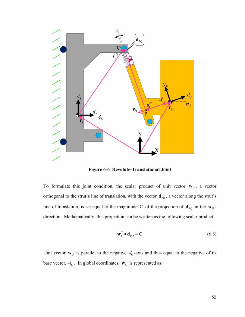
c

U

Figure 6-6 Revolute-Translational Joint

To formulate this joint condition, the scalar product of unit vector , a vector

orthogonal to the strut’s line of translation, with the vector , a vector along the strut’s

line of translation, is set equal to the magnitude of the projection of in the -

direction. Mathematically, this projection can be written as the following scalar product:

Uw

PQ

PQd

C d Uw

TU PQ C• =w d (6.8)

Unit vector is parallel to the negative Uw Ux′ -axis and thus equal to the negative of its

base vector, . In global coordinates, is represented as: U-i Uw

′-i

QS′s

PUr

Sr

PU′s

Q

X

Y

Ux′

U

PQd

Uy′

Sy′φ

UwSφ

Sx′

55

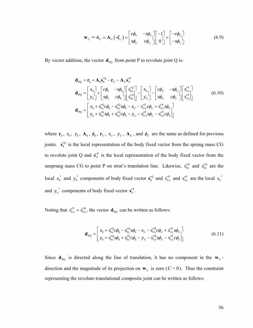
( ) U UU U U U

U U U

10

c s cs c s

Uφ φ φφ φ φ

− −−⎡ ⎤ ⎡⎡ ⎤′= = =⎤

⎢ ⎥ ⎢⎢ ⎥ −⎣ ⎦⎥

⎣ ⎦ ⎣w = -i A -i

⎦ (6.9)

By vector addition, the vector from point P to revolute joint Q is: PQd

Q PPQ S S S U U U

Q PS S S U U USx Ux

PQ Q PS S S U U USy Uy

Q Q P PS Sx S Sy S U Ux U Uy U

PQ Q Q PS Sx S Sy S U Ux

x c s x c ss sy s c y s cs s

x s c s s x s c s sy s s s c y s s


φ φ φ φφ φ φ

′ ′= + − −

⎡ ′ ⎤ ⎡ ′ ⎤− −⎡ ⎤ ⎡ ⎤ ⎡ ⎤ ⎡ ⎤= + − −⎢ ⎥⎢ ⎥ ⎢ ⎥ ⎢ ⎥ ⎢ ⎥ ⎢ ⎥′ ′⎢ ⎥ ⎢⎣ ⎦ ⎣ ⎦ ⎣ ⎦ ⎣ ⎦ ⎥⎣ ⎦ ⎣

′ ′ ′ ′+ − − − +=

′ ′ ′+ + − −

d r A s r A s

d

d PU Uy Us cφ

⎡ ⎤⎢ ⎥′−⎢ ⎥⎣ ⎦

⎦ (6.10)

where , Sr Sx , Sy , , SA Sφ , , Ur Ux , Uy , , and UA Uφ are the same as defined for previous

joints. is the local representation of the body fixed vector from the sprung mass CG

to revolute joint Q and is the local representation of the body fixed vector from the

unsprung mass CG to point P on strut’s translation line. Likewise, and

QS′s

PU′s

QSxs′ Q

Sys′ are the

local Sx ′ and components of body fixed vector Sy ′ QS′s and P

Uxs′ and are the local PUys′ Ux ′

and components of body fixed vector U′y P

U′s .

Noting that PUx U

Bxs s′ = ′ , the vector can be written as follows: PQd

Q Q B P

S Sx S Sy S U U U Uy UPQ Q Q B P

S Sx S Sy S U U U Uy U

x

x


φ φ φ φφ φ φ

⎡ ′ ′ ′ ′+ − − − += ⎢ ⎥′ ′ ′ ′+ + − − −⎢ ⎥⎣ ⎦

dφ

⎤ (6.11)

Since is directed along the line of translation, it has no component in the -

direction and the magnitude of its projection on is zero ( C = 0). Thus the constraint

representing the revolute-translational composite joint can be written as follows:

PQd Uw

Uw

56

(6.12)

[ ]

( )

RT TU PQ

Q Q B PS Sx S Sy S U U U Uy URT

U U Q Q B PS Sx S Sy S U U U Uy U

RT Q Q B PU S Sx S Sy S U U U Uy U

QU S Sx

0

0 0

...

x

x

x

Cx s c s s x s c s s

c sy s s s c y s s s c

c x s c s s x s c s s

s y s s

φ φ φ φφ φ

φ φ φ φ

φ φ φ φ φ

φ

Φ = • − =⎡ ′ ′ ′ ′ ⎤+ − − − +

Φ = − − • − =⎢ ⎥′ ′ ′ ′+ + − − −⎢ ⎥⎣ ⎦

′ ′ ′ ′Φ = − + − − − + −

′+

w d

( )Q B PS Sy S U U U Uy U 0xs c y s s s cφ φ φ φ′ ′ ′+ − − − =

6.6 Driving Constraint

The actuator coordinate Ay is the driven DOF. In general, this driven DOF could be a

function of time and the model’s coordinates: ( )A S S S C C C U U, , , , , , , , ,y f t x y x y x y Uφ φ φ=

( )A

.

For this model the actuator position is a function only of time: y f t= , thus the

driving constraint is:

( )DA 0y f t⎡ ⎤Φ = − =⎣ ⎦ (6.13)

6.7 Complete Constraint Vector

The complete constraint vector is a combination of the kinematic and driving constraints:

S

SA A A A

t S Sx S Sy S C C C Cy CA A A A

RA S Sx S Sy S C C C Cy CK B B B B

RB C C C C C U U U U UD B B B

RT C C C C C U U

D

x

x

x y x y

x y x

xx s c s s x s c s sy s s s c y s s s cx s c s s x s c s sy s s s c y s s

φ

φ φ φ φφ φ φ φφ φ φ φφ φ

′ ′ ′ ′+ − − − +⎡ ⎤

′ ′ ′ ′+ + − − −⎢ ⎥⎢ ⎥⎡ ⎤ ′ ′ ′ ′+ − − − +⎢ ⎥= = =⎢ ⎥

′ ′ ′⎢ ⎥ + + − −⎣ ⎦ Φ⎢ ⎥⎢ ⎥Φ⎣ ⎦

ΦΦ

ΦΦ Φ

Φ

( )( )

( )

BU U U

Q Q B PU S Sx S Sy S U U U Uy U

Q Q B PU S Sx S Sy S U U U Uy U

A

0

...

y

x

x

s c

c x s c s s x s c s s

s y s s s c y s s s c

y f t

φ φ

φ φ φ φ φ

φ φ φ φ φ

⎡ ⎤⎢ ⎥⎢ ⎥⎢ ⎥⎢ ⎥⎢ ⎥⎢ ⎥

=⎢ ⎥′−⎢ ⎥

⎢ ⎥⎧ ⎫′ ′ ′ ′− + − − − + −⎢ ⎥⎪ ⎪⎨ ⎬⎢ ⎥′ ′ ′ ′+ + − − −⎪ ⎪⎢ ⎥⎩ ⎭⎢ ⎥−⎣ ⎦

(6.14)

57

For notational compactness the constants are re-named and substituted into Φ as follows:

(6.15)

ASxA

Sy SA

C SA

Cy S S S C C CB

C S S S C C CB

C C C C U U UB

U C C C U U UB

U U S S SQ

SxQ

Sy

PUy

defg d e f gh d e f gi h i j kj h i j k

k l m

l

m

n

x

x

y

x

y

sss xs x c s x c ss y s c y s cs x c s x c ss y s c y s cs c x c s x

s

s

s

φ

φ φ φ φφ φ φ φφ φ φ φφ φ φ φ

φ φ φ

′=′=′=′= + − − − +′= + + − − −′= + − − − +⇒′= + + − − −′= − + − −

′=

′=

′=

( )( )

( )

U U U

U S S S U U U

A

0

j n ...

l m j n

c s

s y s c y s c

y f t

φ φ

φ φ φ φ φ

⎡ ⎤⎢ ⎥⎢ ⎥⎢ ⎥⎢ ⎥⎢ ⎥⎢ ⎥ =⎢ ⎥⎢ ⎥⎢ ⎥⎧ ⎫− + −⎪ ⎪⎢ ⎥⎨ ⎬⎢ ⎥+ + − − −⎪ ⎪⎩ ⎭⎢ ⎥⎢ ⎥−⎣ ⎦

The Jacobian of this constraint vector is:

(6.16)

S S C C

S S C Cq

C C U U

C C U U

U U 1 U U 2

1

0 0 1 0 0 0 0 0 01 0 0 0 0 0 0 0 01 0 d e 1 0 f g 0 0 00 1 d e 0 1 f g 0 0 00 0 0 1 0 h i 1 0 j k0 0 0 0 1 h i 0 1 j k

R 0 0 0 R0 0 0 0 0 0 0 0 0

R l

s c s cc s c s

s c s cc s c s

c s c s

s



φ φ φ φ

φ

⎡ ⎤⎢ ⎥⎢ ⎥⎢ ⎥− − − +⎢ ⎥− − − +⎢ ⎥= ⎢ ⎥− − − +⎢ ⎥

− − − +⎢ ⎥⎢ ⎥− −⎢ ⎥⎢ ⎥⎣ ⎦

= −

Φ

( ) ( )( ) ( )

U S U S

2 s U U S U S u U s U u U

m

R x l m x y y

c

s s c s c c

φ φ φ

φ φ φ φ φ φ φ φ

+ + − +

= − − + − − + − − +

00000001

This Jacobian has full-row rank, and therefore the constraint equations are independent;

that is, the system is not over-constrained.

58

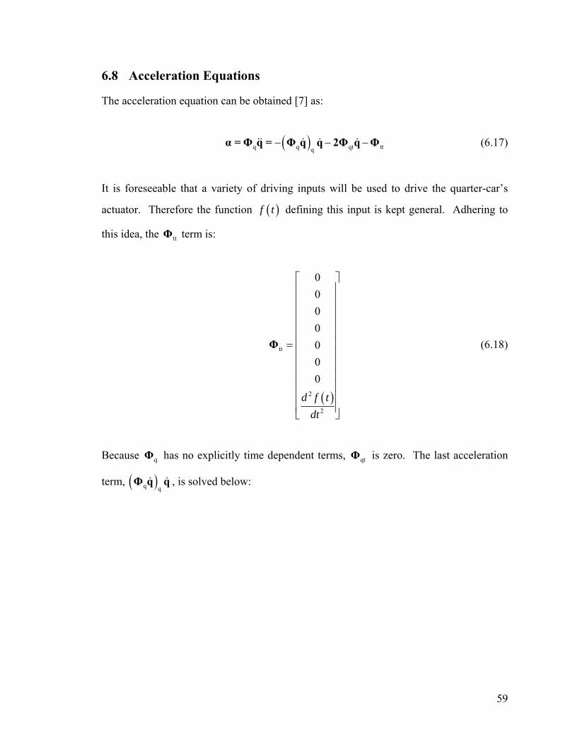
6.8 Acceleration Equations

The acceleration equation can be obtained [7] as:

( )q q qtq− − −α = Φ q = Φ q q 2Φ q Φ&& & & & tt (6.17)

It is foreseeable that a variety of driving inputs will be used to drive the quarter-car’s

actuator. Therefore the function ( )f t defining this input is kept general. Adhering to

this idea, the term is: ttΦ

( )

tt

2

2

0000000

d f tdt

⎡ ⎤⎢ ⎥⎢ ⎥⎢ ⎥⎢ ⎥⎢ ⎥⎢ ⎥=⎢ ⎥⎢ ⎥⎢ ⎥⎢ ⎥⎢ ⎥⎢ ⎥⎣ ⎦

Φ (6.18)

Because has no explicitly time dependent terms, is zero. The last acceleration

term, , is solved below:

qΦ

( q qq&

qtΦ

)Φ q&

59

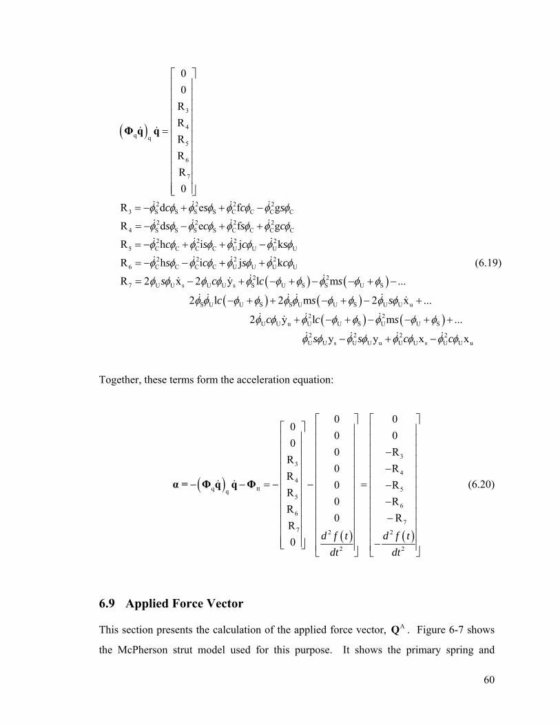
(6.19)

( )3

4q q

5

6

7

2 2 2 23 S S S S C C C C

2 2 2 24 S S S S C C C C

2 2 2 25 C C C C U U U U

2 2 26 C C C C U

00

RRRR R0

R d e f g

R d e f g

R h i j k

R h i

c s c s

s c s c

c s c s

s c




φ φ φ φ φ

⎡ ⎤⎢ ⎥⎢ ⎥⎢ ⎥⎢ ⎥⎢ ⎥= ⎢ ⎥⎢ ⎥⎢ ⎥⎢ ⎥⎢ ⎥⎢ ⎥⎣ ⎦

= − + + −

= − − + +

= − + + −

= − − +

Φ q q& &

& & & &

& & & &

& & & &

& & &

( ) ( )( ) ( )

2U U U

2 27 U U s U U s S U S S U S

S U U S S U U S U U u

2U U u U

j k

R 2 x 2 y l m ...

2 l 2 m 2 x ...

2 y l

s c

s c c s

c s s

c c

φ φ φ

φ φ φ φ φ φ φ φ φ φ

φ φ φ φ φ φ φ φ φ φ

φ φ φ

+

= − + − + − − + −

− + + − + − +

+

&

& && &

& & & & & &

& && ( ) ( )2U S U U S

2 2 2 2U U s U U u U U s U U

m ...

y y x x

s

s s c c

φ φ φ φ φ


− + − − + +

− + −

&

& & & &u

Together, these terms form the acceleration equation:

( )

( ) ( )

33

44

q tt 5q5

66

77 2 2

2 2

0 00

0 00

0 RR

0 RR

0 RR

0 RR

0 R R0 d f t d f t

dt dt

⎡ ⎤ ⎡ ⎤⎡ ⎤ ⎢ ⎥ ⎢ ⎥⎢ ⎥ ⎢ ⎥ ⎢ ⎥⎢ ⎥ ⎢ ⎥ ⎢ ⎥−⎢ ⎥ ⎢ ⎥ ⎢ ⎥−⎢ ⎥ ⎢ ⎥ ⎢ ⎥⎢ ⎥ ⎢ ⎥ ⎢ ⎥− − = − − = −⎢ ⎥ ⎢ ⎥ ⎢ ⎥⎢ ⎥ −⎢ ⎥ ⎢ ⎥⎢ ⎥ ⎢ ⎥ ⎢ ⎥−⎢ ⎥ ⎢ ⎥ ⎢ ⎥⎢ ⎥ ⎢ ⎥ ⎢ ⎥⎢ ⎥ −⎣ ⎦ ⎢ ⎥ ⎢ ⎥⎣ ⎦ ⎣ ⎦

α = Φ q q Φ& & (6.20)

6.9 Applied Force Vector

This section presents the calculation of the applied force vector, . Figure 6-7 shows

the McPherson strut model used for this purpose. It shows the primary spring and

AQ

60

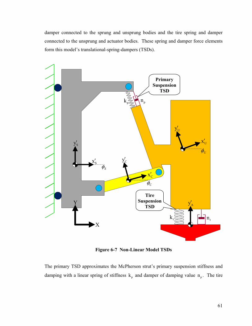
damper connected to the sprung and unsprung bodies and the tire spring and damper

connected to the unsprung and actuator bodies. These spring and damper force elements

form this model’s translational-spring-dampers (TSDs).

Primary Suspension

TSD

pnpk

Uy′

Ux′Sy′

Uφ

Cy′Sx′

Sφ

Cx′

Cφ

Tire Suspension

TSD Ay′Y

tk tnX

Figure 6-7 Non-Linear Model TSDs

The primary TSD approximates the McPherson strut’s primary suspension stiffness and

damping with a linear spring of stiffness pk and damper of damping value pn . The tire

61

TSD approximates the tire’s stiffness and damping with a linear spring of stiffness tk

and damper of damping value nt .

The following sections symbolically solve for the non-linear model’s force vector, Q .

To begin with, forces corresponding to the primary and tire TSDs are developed. Next,

individual force vectors are assembled from the sums of the forces and torques acting on

each body. Lastly, the complete force vector is populated from each body’s

individual force vector.

A

AQ

62

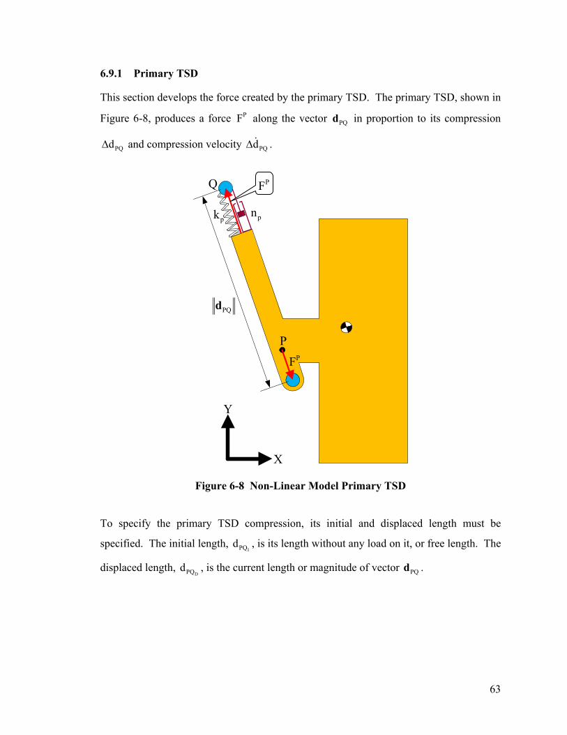
6.9.1 Primary TSD

This section develops the force created by the primary TSD. The primary TSD, shown in

Figure 6-8, produces a force along the vector in proportion to its compression

and compression velocity .

PF

Δ

PQd

PQdΔ PQd&

PFQ

pnpk

PQd

PPF

Y

X

Figure 6-8 Non-Linear Model Primary TSD

To specify the primary TSD compression, its initial and displaced length must be

specified. The initial length, d , is its length without any load on it, or free length. The

displaced length, d , is the current length or magnitude of vector .

IPQ

DPQ PQd

63

( )

D

D

D

PQ PQ

Q Q B PS Sx S Sy S U U U Uy U

PQ Q Q B PS Sx S Sy S U U U Uy U

2Q Q B PS Sx S Sy S U U U Uy U

PQQ Q B P

S Sx S Sy S U U U Uy

Displaced length d

d

d

x

x

x

x


x s c s s x s c s s

y s s s c y s s s c


φ φ φ φ

φ φ φ

= = =

′ ′ ′ ′+ − − − +=

′ ′ ′ ′+ + − − −

′ ′ ′ ′+ − − − +=

′ ′ ′ ′+ + − − −

d

( )+

2

Uφ

(6.21)

Thus the primary TSD compression is:

( )( )I

PQ

2Q Q B PS Sx S Sy S U U U Uy U

PQ PQ 2Q Q B PS Sx S Sy S U U U Uy U

d Initial length Displaced length

d dx

x

x s c s s x s c s s

y s s s c y s s s c

φ φ φ φ

φ φ φ φ

Δ = −

′ ′ ′ ′+ − − − +Δ = −

′ ′ ′ ′+ + − − −

+ (6.22)

The first time derivative of vector is the primary TSD’s compression velocity vector: PQd

Q Q B P

S S Sx S S Sy S U U U U U Uy UPQ Q Q B P

S S Sx S S Sy S U U U U U Uy U

x

x

x s s s c x s s s cy s c s s y s c s s

φ φ φ φ φ φ φ φφ φ φ φ φ φ φ φ

⎡ ⎤′ ′ ′ ′− − − + += ⎢ ⎥′ ′ ′ ′+ − − − +⎢ ⎥⎣ ⎦

d& & & && &

&& & & && &

(6.23)

By multiplying the magnitude of this vector by SIGN the compressive velocity can be

written as the following scalar:

( )( )

PQ PQ

2Q Q B PS S Sx S S Sy S U U U U U Uy U

PQ 2Q Q B PS S Sx S S Sy S U U U U U Uy U

d

dx

x

x s s s c x s s s c

y s c s s y s c s s



Δ = ×

′ ′ ′ ′− − − + +Δ = ×

′ ′ ′ ′+ − − − +

SIGN d

SIGN

& &

& & & && &&

& & & && &

+ (6.24)

SIGN is positive when the TSD is compressing (that is, when the current TSD length is

less than the previous). This SIGN convention supports the assumption that a positive

TSD damper force is an outward force from its center towards points Q and P.

64

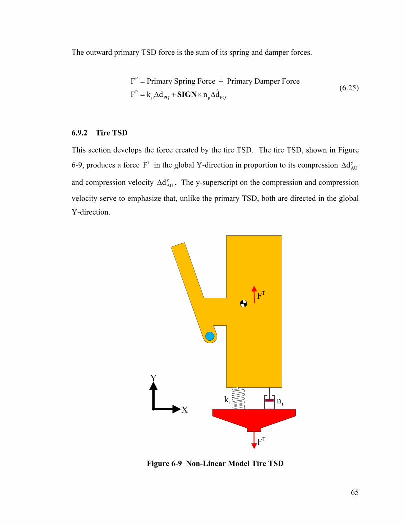
The outward primary TSD force is the sum of its spring and damper forces.

(6.25) P

Pp PQ p PQ

F Primary Spring Force Primary Damper Force

F k d n d

= +

= Δ + × ΔSIGN &

6.9.2 Tire TSD

This section develops the force created by the tire TSD. The tire TSD, shown in Figure

6-9, produces a force in the global Y-direction in proportion to its compression

and compression velocity . The y-superscript on the compression and compression

velocity serve to emphasize that, unlike the primary TSD, both are directed in the global

Y-direction.

TF yAUdΔ

yAUdΔ&

TF

Y

tktn

X

TF

Figure 6-9 Non-Linear Model Tire TSD

65

To specify the tire TSD compression, its initial and displaced length must be specified.

The initial length, , is its length without any load on it, or free length. The displaced

length is the global unsprung mass Y-position minus the actuator Y-position. Thus, the

tire TSD compression is:

I

yAUd

(6.26) ( )

I

yAUy yAU AU U A

d Initial length Displaced length

d d y y

Δ = −

Δ = − −

Positive spring forces are applied outward from the TSD’s center towards the unsprung

mass and actuator when the spring is compressed.

The first time derivative of tire TSD compression is the tire TSD compression velocity:

yAU U Ad y yΔ = − +& & & (6.27)

Positive damper forces are applied outward from the TSD’s center toward the unsprung

mass and actuator when the damper is compressing. The red vectors in Figure 6-9 show

the positive tire TSD force direction. The outward tire TSD force is the sum of its spring

and damper forces:

(6.28) T

T y yt AU t AU

F Tire Spring Force Tire Damper Force

F k d n d

= +

= Δ + Δ&

6.9.3 Sprung Mass Forces

This section identifies the applied sprung mass forces. Figure 6-10 shows the location of

these forces on the sprung mass. The forces acting on this body are due to the primary

TSD and gravity.

66

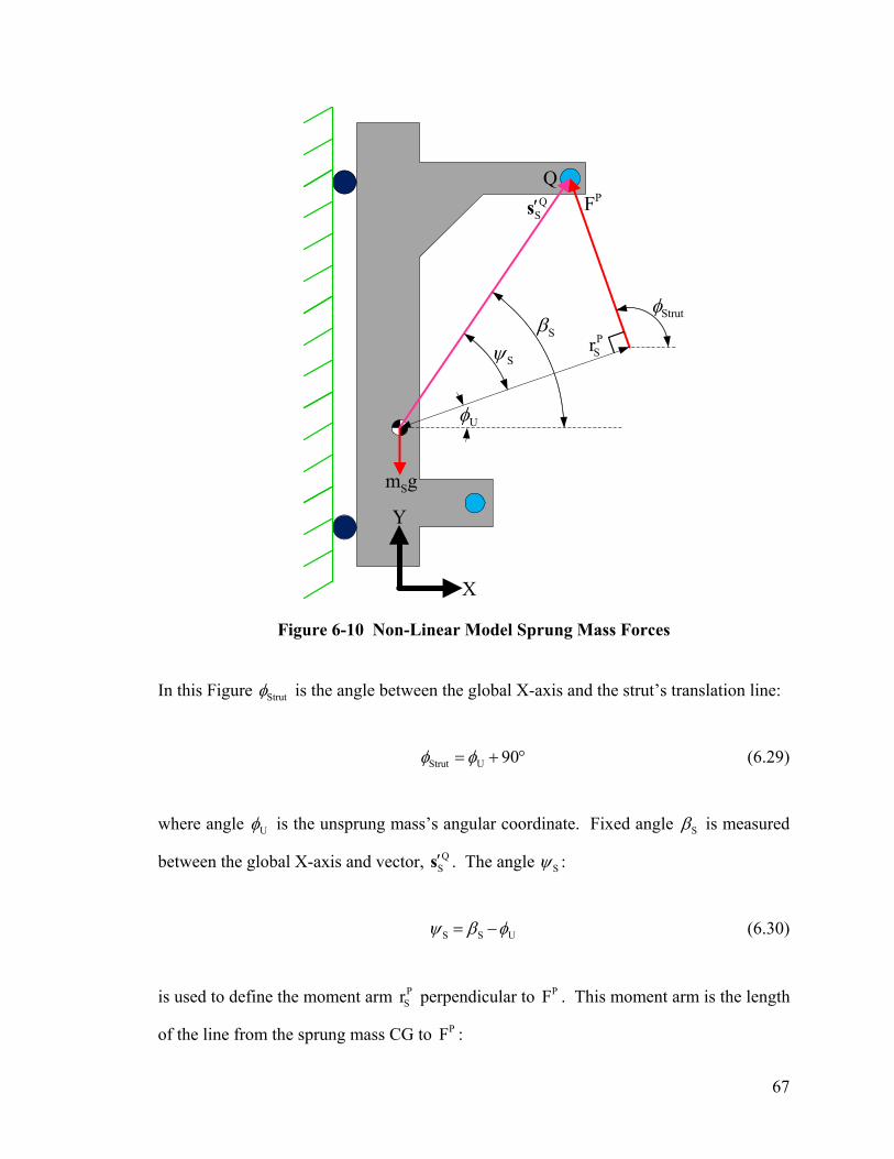
QS′s

Figure 6-10 Non-Linear Model Sprung Mass Forces

In this Figure Strutφ is the angle between the global X-axis and the strut’s translation line:

Strut U 90φ φ= + ° (6.29)

where angle Uφ is the unsprung mass’s angular coordinate. Fixed angle Sβ is measured

between the global X-axis and vector, QS′s . The angle Sψ :

S S Uψ β φ= − (6.30)

is used to define the moment arm perpendicular to . This moment arm is the length

of the line from the sprung mass CG to

PSr

PF

PF :

Y

Sψ

Uφ

Sβ

QPF

Sm g

X

StrutφP

Sr

67

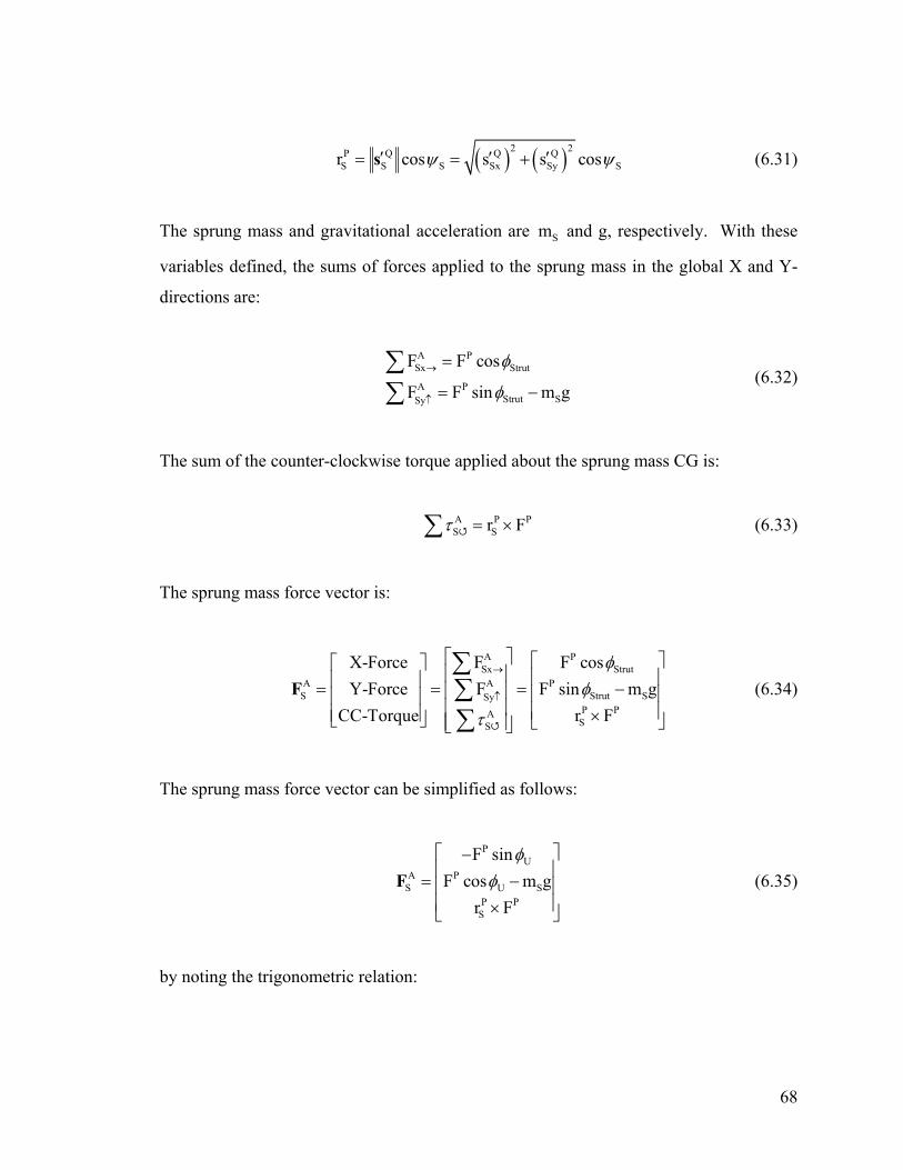
( ) ( )2 2P Q Q QS S S Sx Syr cos s s cos Sψ ψ′ ′ ′= = +s (6.31)

The sprung mass and gravitational acceleration are and g, respectively. With these

variables defined, the sums of forces applied to the sprung mass in the global X and Y-

directions are:

Sm

A P

Sx Strut

A PStrut SSy

F F cos

F F sin m

φ

φ→

↑

=

= − g∑∑

(6.32)

The sum of the counter-clockwise torque applied about the sprung mass CG is:

A PS Sr Fτ P= ×∑ (6.33)

The sprung mass force vector is:

A PSx Strut

A A PS Sy

P PASS

X-Force F F cosY-Force F F sin m g

CC-Torque r F

φφ

τ

→

↑

⎡ ⎤

Strut S

⎡ ⎤⎡ ⎤⎢ ⎥ ⎢ ⎥⎢ ⎥= = = −⎢ ⎥ ⎢ ⎥⎢ ⎥⎢ ⎥ ⎢ ⎥⎢ ⎥ ×⎣ ⎦ ⎣ ⎦⎢ ⎥⎣ ⎦

∑∑∑

F (6.34)

The sprung mass force vector can be simplified as follows:

PU

A PS U

P PS

F sinF cos m g

r F

φφ S

⎡ ⎤−⎢ ⎥= −⎢ ⎥⎢ ⎥×⎣ ⎦

F (6.35)

by noting the trigonometric relation:

68

( )( )

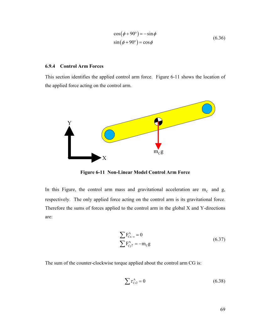
cos 90 sin

sin 90 cos

φ φ

φ φ

+ ° = −

+ ° = (6.36)

6.9.4 Control Arm Forces

This section identifies the applied control arm force. Figure 6-11 shows the location of

the applied force acting on the control arm.

Y

Cm gX

Figure 6-11 Non-Linear Model Control Arm Force

In this Figure, the control arm mass and gravitational acceleration are and g,

respectively. The only applied force acting on the control arm is its gravitational force.

Therefore the sums of forces applied to the control arm in the global X and Y-directions

are:

Cm

ACx

ACCy

F 0

F m→

↑

=

= − g∑∑

(6.37)

The sum of the counter-clockwise torque applied about the control arm CG is:

AC 0τ =∑ (6.38)

69

The control arm force vector is:

ACx

A AC Cy

AC

X-Force F 0Y-Force F m g

CC-Torque 0τ

→

↑

⎡ ⎤

C

⎡ ⎤ ⎡⎢ ⎥

⎤⎢ ⎥ ⎢= = = −⎢ ⎥

⎥⎢ ⎥ ⎢

⎢ ⎥⎥

⎢ ⎥ ⎢ ⎥⎣ ⎦ ⎣⎢ ⎥⎣ ⎦

∑∑∑

F

⎦

(6.39)

6.9.5 Unsprung Mass Forces

This section identifies the applied unsprung mass forces. Figure 6-12 shows the location

of these forces on the unsprung mass. The forces acting on this body are due to the

primary and tire TSDs and gravity.

PF

BUxs′

Um g

TUr

Y

XTF

Figure 6-12 Non-Linear Model Unsprung Mass Forces

70

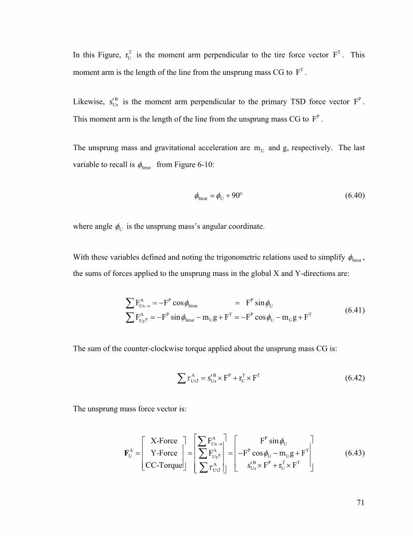
In this Figure, is the moment arm perpendicular to the tire force vector . This

moment arm is the length of the line from the unsprung mass CG to .

TUr

TF

TF

Likewise, BUxs′ is the moment arm perpendicular to the primary TSD force vector .

This moment arm is the length of the line from the unsprung mass CG to

PF

PF .

The unsprung mass and gravitational acceleration are and g, respectively. The last

variable to recall is

Um

Strutφ from Figure 6-10:

Strut U 90φ φ= + ° (6.40)

where angle Uφ is the unsprung mass’s angular coordinate.

With these variables defined and noting the trigonometric relations used to simplify Strutφ ,

the sums of forces applied to the unsprung mass in the global X and Y-directions are:

(6.41) A P PUx Strut U

A P T PStrut U U UUy

F F cos F sin

F F sin m g F F cos m g

φ φ

φ φ→

↑

= − =

= − − + = − − +

∑∑ TF

T

The sum of the counter-clockwise torque applied about the unsprung mass CG is:

A B P TU U UF r Fxsτ ′= × + ×∑ (6.42)

The unsprung mass force vector is:

A PUx U

A A PU UUy

B P T TAU UU

X-Force F F sinY-Force F F cos m g F

CC-Torque F r Fxs

φφ

τ

→

↑

⎡ ⎤T

U

⎡ ⎤⎡ ⎤⎢ ⎥ ⎢ ⎥⎢ ⎥= = = − −⎢ ⎥ +⎢ ⎥⎢ ⎥⎢ ⎥ ⎢ ⎥′⎢ ⎥ × + ×⎣ ⎦ ⎣ ⎦⎢ ⎥⎣ ⎦

∑∑∑

F (6.43)

71

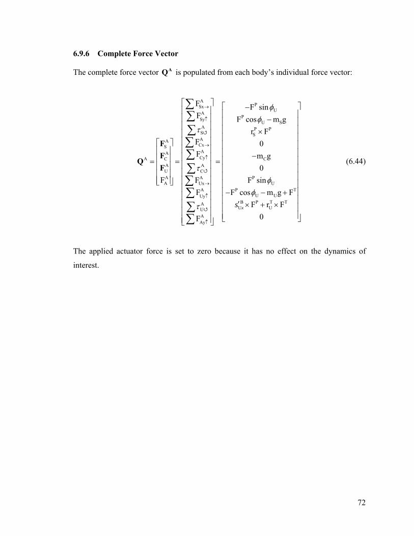
6.9.6 Complete Force Vector

The complete force vector is populated from each body’s individual force vector: AQ

APSx

UAPSy U S

A P PS SAACxSAACyA C C

A AU CA A PA Ux U

A PU UUy

B P T TAU UU

AAy

F F sinF F cos m g

r FF 0F m g

0F F F sin

F F cos m gF r F

0Fxs

φφ

τ

τφ

φ

τ

→

↑

→

↑

→

↑

↑

⎡ ⎤ ⎡ −⎢ ⎥ ⎢⎢ ⎥ −⎢⎢ ⎥ ⎢ ×⎢ ⎥ ⎢⎢ ⎥⎡ ⎤ ⎢⎢ ⎥⎢ ⎥ ⎢ −⎢ ⎥⎢ ⎥ ⎢= = =⎢ ⎥⎢ ⎥⎢ ⎥⎢ ⎥⎢ ⎥⎢ ⎥⎣ ⎦⎢ ⎥ − − +⎢ ⎥

′⎢ ⎥ × + ×⎢ ⎥

⎣⎢ ⎥⎣ ⎦

TF

∑∑∑∑∑∑∑∑∑∑

FF

QF

⎤⎥⎥⎥⎥⎥⎥⎥

⎢ ⎥⎢ ⎥⎢ ⎥⎢ ⎥⎢ ⎥⎢ ⎥⎢ ⎥⎦

(6.44)

The applied actuator force is set to zero because it has no effect on the dynamics of

interest.

72

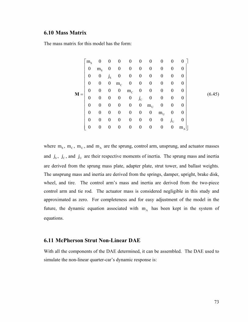
6.10 Mass Matrix

The mass matrix for this model has the form:

(6.45)

S

S

S

C

C

C

U

U

U

A

m 0 0 0 0 0 0 0 0 00 m 0 0 0 0 0 0 0 00 0 0 0 0 0 0 0 00 0 0 m 0 0 0 0 0 00 0 0 0 m 0 0 0 0 00 0 0 0 0 0 0 0 00 0 0 0 0 0 m 0 0 00 0 0 0 0 0 0 m 0 00 0 0 0 0 0 0 0 00 0 0 0 0 0 0 0 0 m

j

j

j

⎡ ⎤⎢ ⎥⎢ ⎥⎢ ⎥⎢ ⎥⎢ ⎥⎢ ⎥

= ⎢ ⎥⎢ ⎥⎢ ⎥⎢ ⎥⎢ ⎥⎢ ⎥⎢ ⎥⎢ ⎥⎣ ⎦

M

where , and are the sprung, control arm, unsprung, and actuator masses

and

Sm ,

S

Cm , Um Am

j , Cj , and Uj are their respective moments of inertia. The sprung mass and inertia

are derived from the sprung mass plate, adapter plate, strut tower, and ballast weights.

The unsprung mass and inertia are derived from the springs, damper, upright, brake disk,

wheel, and tire. The control arm’s mass and inertia are derived from the two-piece

control arm and tie rod. The actuator mass is considered negligible in this study and

approximated as zero. For completeness and for easy adjustment of the model in the

future, the dynamic equation associated with has been kept in the system of

equations.

Am

6.11 McPherson Strut Non-Linear DAE

With all the components of the DAE determined, it can be assembled. The DAE used to

simulate the non-linear quarter-car’s dynamic response is:

73

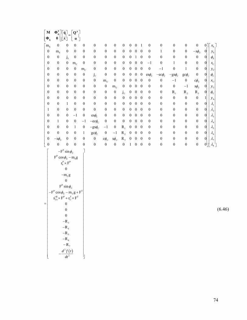
S

S U

S

C

C

C C C C C

U U

U

m 0 0 0 0 0 0 0 0 0 0 1 0 0 0 0 0 00 m 0 0 0 0 0 0 0 0 0 0 0 1 0 0 00 0 0 0 0 0 0 0 0 1 0 0 0 0 0 0 00 0 0 m 0 0 0 0 0 0 0 0 1 0 1 0 0 00 0 0 0 m 0 0 0 0 0 0 0 0 1 0 1 0 00 0 0 0 0 0 0 0 0 0 0 e e g g 0 00 0 0 0 0 0 m 0 0 0 0 0 0 0 1 0 00 0 0 0 0 0 0 m 0

sj

j s c s cc

φ

φ φ φ φφ

⎡ ⎤ ⎡ ⎤⎡ ⎤⎢ ⎥ ⎢ ⎥⎢ ⎥⎢ ⎥ ⎣ ⎦ ⎣ ⎦⎣ ⎦

−

−−

− −−

T Aq

q

M Φ q Q=

Φ 0 λ α&&

U

U 1 2

C

C

C 1

C 2

U U U 3

0 0 0 0 0 0 1 00 0 0 0 0 0 0 0 0 0 0 0 0 R R R 00 0 0 0 0 0 0 0 0 0 0 0 0 0 0 0 0 10 0 1 0 0 0 0 0 0 0 0 0 0 0 0 0 0 01 0 0 0 0 0 0 0 0 0 0 0 0 0 0 0 0 00 0 0 1 0 e 0 0 0 0 0 0 0 0 0 0 0 00 1 0 0 1 e 0 0 0 0 0 0 0 0 0 0 0 00 0 0 1 0 g 1 0 R 0 0 0 0 0 0 0 0 00 0 0 0 1 g 0 1 R 0 0 0 0 0 0 0 0 00 0 0 0 0 R 0 0 0

sj

scs

cs c s

φ

φφφφ

φ φ φ

−

−− −

− −−

−

S

S

S

C

C

C

U

U

U

A

1

2

3

4

5

6

7

8

PU

PU S

P PS

0 0 0 0 0 00 0 0 0 0 0 0 0 0 1 0 0 0 0 0 0 0 0

F sinF cos m g

r F0

3

xy

xy

xy

y

φ

φ

φ

λλλλλλλλ

φφ

⎡ ⎤⎡ ⎤⎢ ⎥⎢ ⎥⎢ ⎥⎢ ⎥⎢ ⎥⎢ ⎥⎢ ⎥⎢ ⎥⎢ ⎥⎢ ⎥⎢ ⎥⎢ ⎥⎢ ⎥⎢ ⎥⎢ ⎥⎢ ⎥⎢ ⎥⎢ ⎥⎢ ⎥⎢ ⎥⎢ ⎥⎢ ⎥⎢ ⎥⎢ ⎥⎢ ⎥⎢ ⎥⎢ ⎥⎢ ⎥⎢ ⎥⎢ ⎥⎢ ⎥⎢ ⎥⎢ ⎥⎢ ⎥⎢ ⎥⎢ ⎥⎢ ⎥⎢ ⎥⎢ ⎥⎢ ⎥⎢ ⎥⎢ ⎥⎢ ⎥⎢ ⎥⎢ ⎥⎢ ⎥⎢ ⎥⎢ ⎥⎢ ⎥⎢ ⎥⎢ ⎥⎢ ⎥

⎣ ⎦ ⎣ ⎦

−−

×

−

=

( )

C

PU

P TU U

B P T TU U

3

4

5

6

72

2

m g0

F sinF cos m g F

F r F000RRRR

R

xs

d f tdt

φφ

⎡ ⎤⎢ ⎥⎢ ⎥⎢ ⎥⎢ ⎥⎢ ⎥⎢ ⎥⎢ ⎥⎢ ⎥⎢ ⎥⎢ ⎥⎢ ⎥− − +⎢ ⎥′ × + ×⎢ ⎥⎢ ⎥⎢ ⎥⎢ ⎥⎢ ⎥⎢ ⎥

−⎢ ⎥⎢ ⎥−⎢ ⎥

−⎢ ⎥⎢ ⎥−⎢ ⎥⎢ ⎥−⎢ ⎥⎢ ⎥−⎢ ⎥⎣ ⎦

(6.46)

74

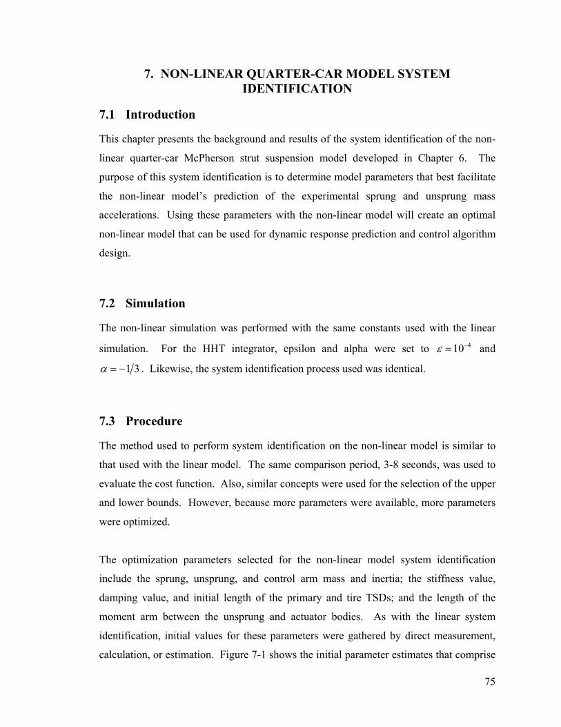
7. NON-LINEAR QUARTER-CAR MODEL SYSTEM IDENTIFICATION

7.1 Introduction

This chapter presents the background and results of the system identification of the non-

linear quarter-car McPherson strut suspension model developed in Chapter 6. The

purpose of this system identification is to determine model parameters that best facilitate

the non-linear model’s prediction of the experimental sprung and unsprung mass

accelerations. Using these parameters with the non-linear model will create an optimal

non-linear model that can be used for dynamic response prediction and control algorithm

design.

7.2 Simulation

The non-linear simulation was performed with the same constants used with the linear

simulation. For the HHT integrator, epsilon and alpha were set to 410ε −= and

1 3α = − . Likewise, the system identification process used was identical.

7.3 Procedure

The method used to perform system identification on the non-linear model is similar to

that used with the linear model. The same comparison period, 3-8 seconds, was used to

evaluate the cost function. Also, similar concepts were used for the selection of the upper

and lower bounds. However, because more parameters were available, more parameters

were optimized.

The optimization parameters selected for the non-linear model system identification

include the sprung, unsprung, and control arm mass and inertia; the stiffness value,

damping value, and initial length of the primary and tire TSDs; and the length of the

moment arm between the unsprung and actuator bodies. As with the linear system

identification, initial values for these parameters were gathered by direct measurement,

calculation, or estimation. Figure 7-1 shows the initial parameter estimates that comprise

75

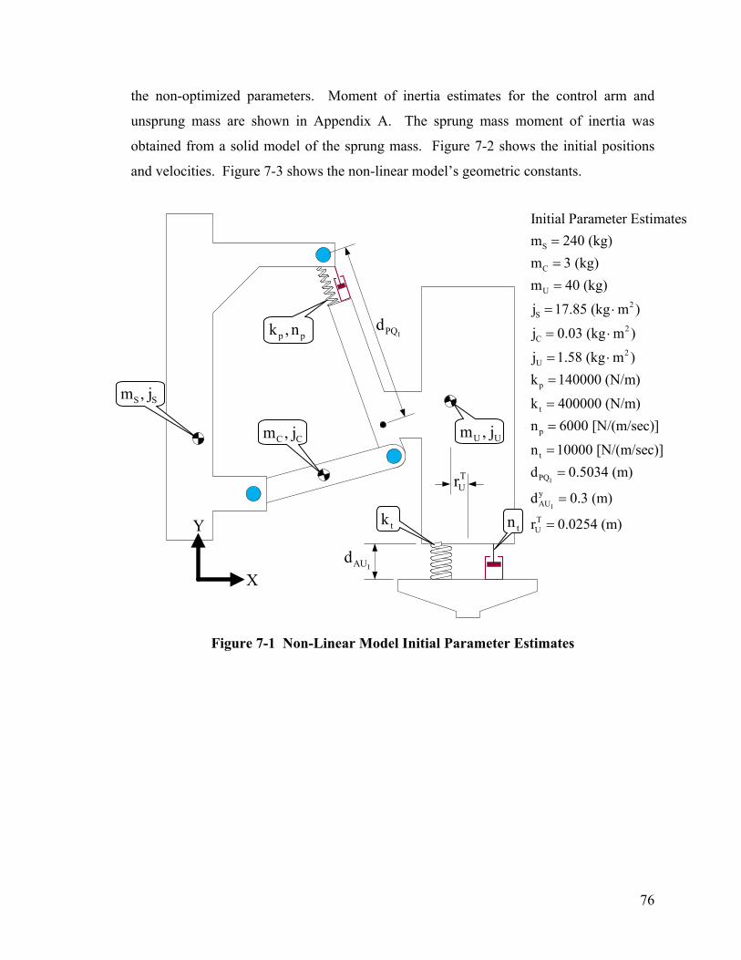
the non-optimized parameters. Moment of inertia estimates for the control arm and

unsprung mass are shown in Appendix A. The sprung mass moment of inertia was

obtained from a solid model of the sprung mass. Figure 7-2 shows the initial positions

and velocities. Figure 7-3 shows the non-linear model’s geometric constants.

I

I

S

C

U

2S

2C

2U

p

t

p

t

PQ

yAU

Initial Parameter Estimatesm 240 (kg)m 3 (kg)m 40 (kg)

j 17.85 (kg m )

j 0.03 (kg m )

j 1.58 (kg m )k 140000 (N/m)

k 400000 (N/m)n 6000 [N/(m/sec)]

n 10000 [N/(m/sec)]d 0.5034 (m)

d 0.3 (m)

=

=

=

= ⋅

= ⋅

= ⋅

=

=

=

=

=

=TUr 0.0254 (m)=

p pk , n IPQd

S Sm , j

U Um , jC Cm , j

TUr

tktnY

IAUdX

Figure 7-1 Non-Linear Model Initial Parameter Estimates

76

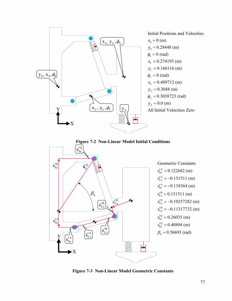
S

S

S

C

C

C

U

U

U

A

Initial Positions and Velocities0 (m)0.28448 (m)0 (rad)0.274193 (m)0.166116 (m)0 (rad)0.489712 (m)0.3048 (m)0.3038723 (rad)0.0 (m)

All Initial Velocities Zero

xy

xy

xy

y

φ

φ

φ

====

====

==

U, U Ux y ,φ

S S Sy , x ,φ

C C Cx , y ,φAy

X

Y

Figure 7-2 Non-Linear Model Initial Conditions

QSxs′

ASx

ACA

Sy

BC

BU

BU

QSx

QSy

S

Geometric Constants0.122682 (m)

0.151511 (m)

0.118364 (m)

0.151511 (m)

0.10257282 (m)

0.11317732 (m)

0.26035 (m)

0.40894 (m)

0.56693 (rad)

x

x

x

y

s

s

s

s

s

s

s

s

β

′ =

′ = −

′ = −

′ =

′ = −

′ = −

′ =

′ =

=

QSys′ Q

S′s

SβB

Uxs′BUys′

BCxs′

ASys′

ACxs′

ASxs′Y

X

Figure 7-3 Non-Linear Model Geometric Constants

77

7.4 Performance Measure

As with the linear model, the performance metric chosen to judge how well the

mathematical model predicts the experimental acceleration is the ratio of the root-mean-

square (RMS) acceleration error to the experimental RMS acceleration over the 3 to 50

second time interval. These ratios, for the sprung and unsprung mass, expressed in

decibel form, are:

( )( )

( )( )

SS

S

UU

U

RMSR 20log10

RMS Exp_a

RMSR 20log10

RMS Exp_a

e

e

⎛ ⎞= ⎜ ⎟⎜ ⎟

⎝⎛ ⎞

= ⎜ ⎟⎜ ⎟⎝ ⎠

⎠ (7.1)

where and are the sprung and unsprung mass performance ratios. As with the

linear model, the lower the ratio, the better the performance.

SR UR

7.5 Non-Linear System Identification Results

Figure 7-4 compares the acceleration predicted by the mathematical model (green –

dashed) using the initial parameter estimates with the experimentally measured

accelerations (blue – solid). The error is highlighted in red (dash – dot). This non-

optimized model produces sprung and unsprung mass performance ratios of:

S

U

R 9.4216 dB R 2.72 dB

= −= −

(7.2)

Figure 7-5 compares the acceleration predicted by the mathematical model using

optimized parameters with the experimentally measured accelerations. This optimized

model produces sprung and unsprung mass performance ratios of:

78

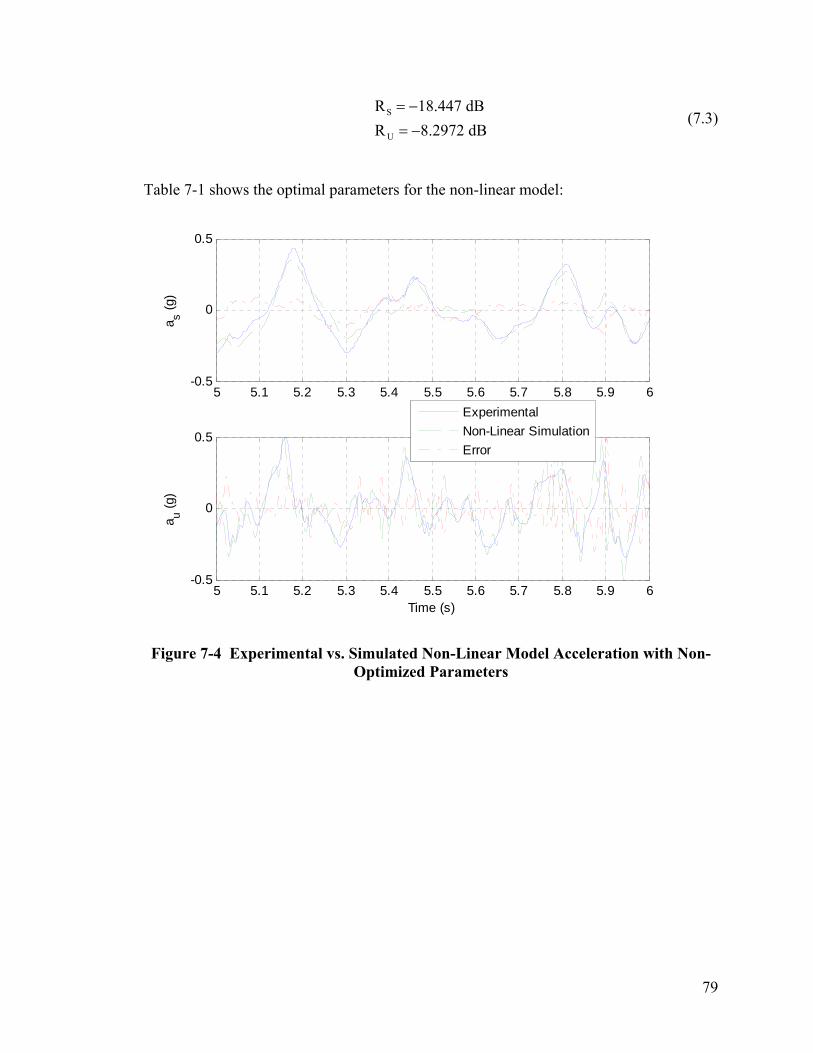
S

U

R 18.447 dBR 8.2972 dB

= −= −

(7.3)

Table 7-1 shows the optimal parameters for the non-linear model:

5 5.1 5.2 5.3 5.4 5.5 5.6 5.7 5.8 5.9 6-0.5

0

0.5

a s (g)

5 5.1 5.2 5.3 5.4 5.5 5.6 5.7 5.8 5.9 6-0.5

0

0.5

a u (g)

Time (s)

ExperimentalNon-Linear SimulationError

Figure 7-4 Experimental vs. Simulated Non-Linear Model Acceleration with Non-Optimized Parameters

79

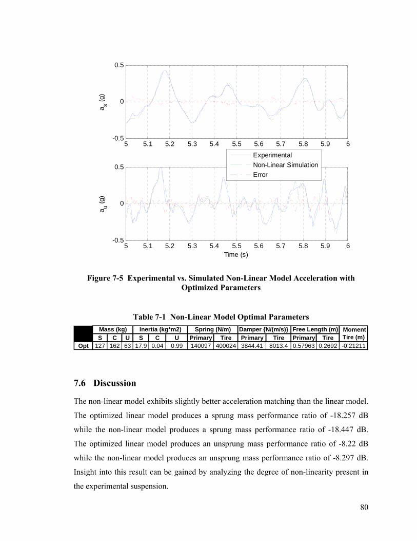
5 5.1 5.2 5.3 5.4 5.5 5.6 5.7 5.8 5.9 6-0.5

0

0.5

a s (g)

5 5.1 5.2 5.3 5.4 5.5 5.6 5.7 5.8 5.9 6-0.5

0

0.5

a u (g)

Time (s)

ExperimentalNon-Linear SimulationError

Figure 7-5 Experimental vs. Simulated Non-Linear Model Acceleration with Optimized Parameters

Table 7-1 Non-Linear Model Optimal Parameters

S C U S C U Primary Tire Primary Tire Primary TireOpt 127 162 63 17.9 0.04 0.99 140097 400024 3844.41 8013.4 0.57963 0.2692 -0.21211

Mass (kg) Inertia (kg*m2) Spring (N/m) Damper {N/(m/s)} Free Length (m) Moment Tire (m)

7.6 Discussion

The non-linear model exhibits slightly better acceleration matching than the linear model.

The optimized linear model produces a sprung mass performance ratio of -18.257 dB

while the non-linear model produces a sprung mass performance ratio of -18.447 dB.

The optimized linear model produces an unsprung mass performance ratio of -8.22 dB

while the non-linear model produces an unsprung mass performance ratio of -8.297 dB.

Insight into this result can be gained by analyzing the degree of non-linearity present in

the experimental suspension.

80

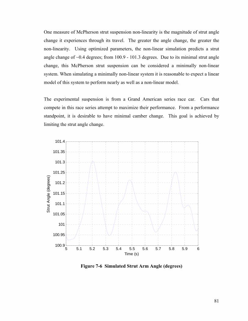
One measure of McPherson strut suspension non-linearity is the magnitude of strut angle

change it experiences through its travel. The greater the angle change, the greater the

non-linearity. Using optimized parameters, the non-linear simulation predicts a strut

angle change of ~0.4 degrees; from 100.9 - 101.3 degrees. Due to its minimal strut angle

change, this McPherson strut suspension can be considered a minimally non-linear

system. When simulating a minimally non-linear system it is reasonable to expect a linear

model of this system to perform nearly as well as a non-linear model.

The experimental suspension is from a Grand American series race car. Cars that

compete in this race series attempt to maximize their performance. From a performance

standpoint, it is desirable to have minimal camber change. This goal is achieved by

limiting the strut angle change.

5 5.1 5.2 5.3 5.4 5.5 5.6 5.7 5.8 5.9 6100.9

100.95

101

101.05

101.1

101.15

101.2

101.25

101.3

101.35

101.4

Stru

t Ang

le (d

egre

es)

Time (s)

Figure 7-6 Simulated Strut Arm Angle (degrees)

81

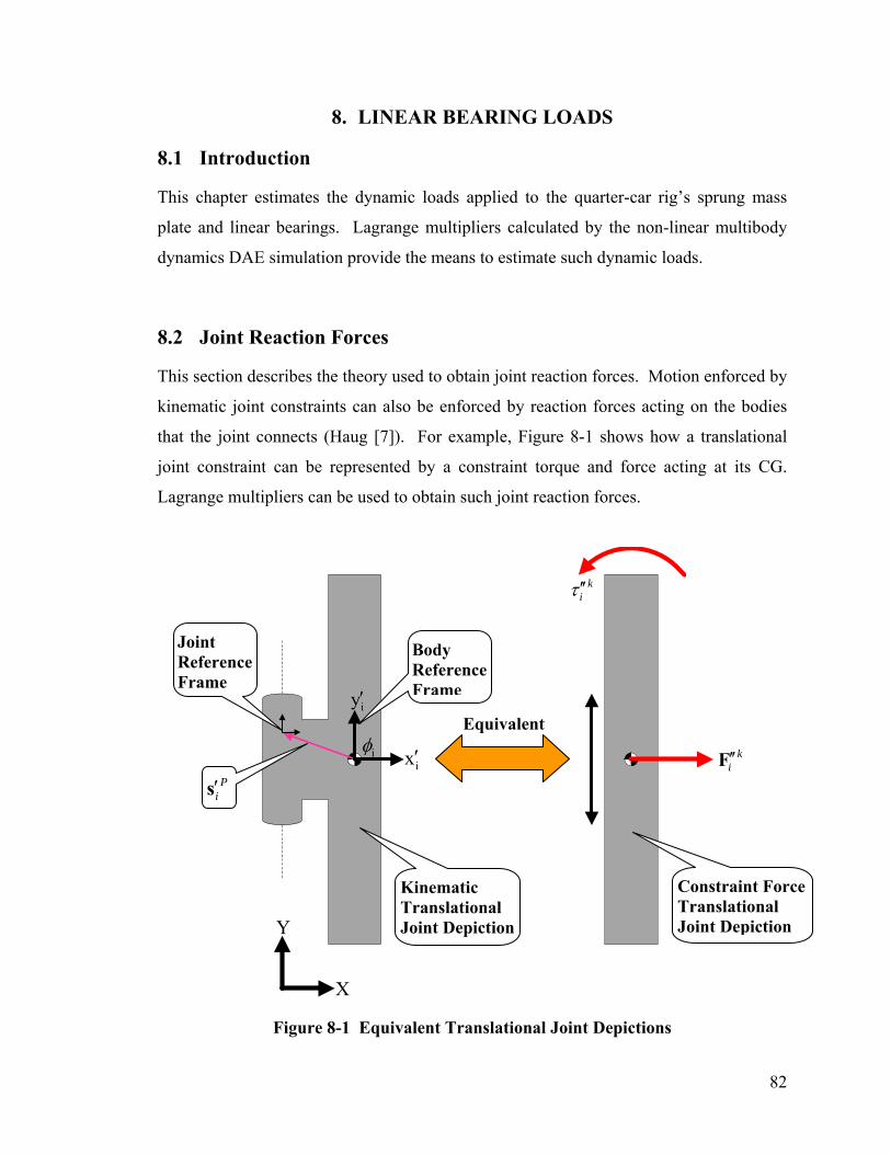
8. LINEAR BEARING LOADS

8.1 Introduction

This chapter estimates the dynamic loads applied to the quarter-car rig’s sprung mass

plate and linear bearings. Lagrange multipliers calculated by the non-linear multibody

dynamics DAE simulation provide the means to estimate such dynamic loads.

8.2 Joint Reaction Forces

This section describes the theory used to obtain joint reaction forces. Motion enforced by

kinematic joint constraints can also be enforced by reaction forces acting on the bodies

that the joint connects (Haug [7]). For example, Figure 8-1 shows how a translational

joint constraint can be represented by a constraint torque and force acting at its CG.

Lagrange multipliers can be used to obtain such joint reaction forces.

kiτ ′′

Joint Reference Frame

Equivalent

ix′iφ

iy′

Body Reference Frame

Pi′s

ki′′F

Kinematic Translational Joint Depiction

Constraint Force Translational Joint DepictionY

X

Figure 8-1 Equivalent Translational Joint Depictions

82

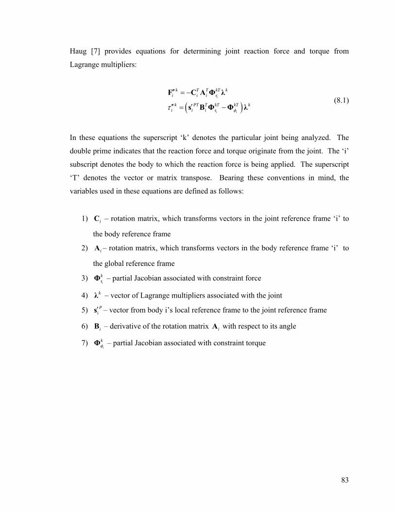
Haug [7] provides equations for determining joint reaction force and torque from

Lagrange multipliers:

(8.1) ( )

i

i i

r

r

k T T kT ki i i

k PT T kT kT ki i i φτ

′′ = −

′′ ′= −

F C A Φ λ

s B Φ Φ λ

In these equations the superscript ‘k’ denotes the particular joint being analyzed. The

double prime indicates that the reaction force and torque originate from the joint. The ‘i’

subscript denotes the body to which the reaction force is being applied. The superscript

‘T’ denotes the vector or matrix transpose. Bearing these conventions in mind, the

variables used in these equations are defined as follows:

1) iC – rotation matrix, which transforms vectors in the joint reference frame ‘i’ to

the body reference frame

2) iA – rotation matrix, which transforms vectors in the body reference frame ‘i’ to

the global reference frame

3) irkΦ – partial Jacobian associated with constraint force

4) kλ – vector of Lagrange multipliers associated with the joint

5) Pi′s – vector from body i’s local reference frame to the joint reference frame

6) iB – derivative of the rotation matrix iA with respect to its angle

7) i

kφΦ – partial Jacobian associated with constraint torque

83

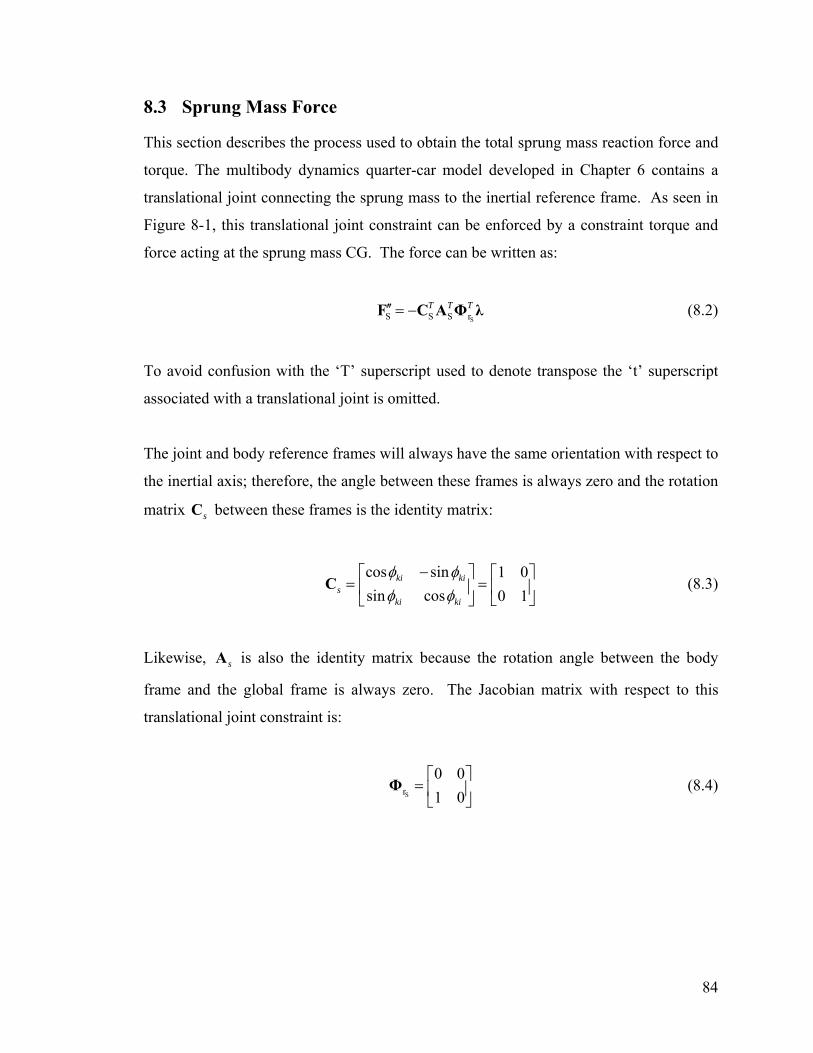
8.3 Sprung Mass Force

This section describes the process used to obtain the total sprung mass reaction force and

torque. The multibody dynamics quarter-car model developed in Chapter 6 contains a

translational joint connecting the sprung mass to the inertial reference frame. As seen in

Figure 8-1, this translational joint constraint can be enforced by a constraint torque and

force acting at the sprung mass CG. The force can be written as:

(8.2) SS S S r

T T T′′ = −F C A Φ λ

To avoid confusion with the ‘T’ superscript used to denote transpose the ‘t’ superscript

associated with a translational joint is omitted.

The joint and body reference frames will always have the same orientation with respect to

the inertial axis; therefore, the angle between these frames is always zero and the rotation

matrix sC between these frames is the identity matrix:

cos sin 1 0sin cos 0 1

ki kis

ki ki

φ φφ φ

−⎡ ⎤ ⎡ ⎤= ⎢ ⎥ = ⎢ ⎥

⎣ ⎦⎣ ⎦C (8.3)

Likewise, sA is also the identity matrix because the rotation angle between the body

frame and the global frame is always zero. The Jacobian matrix with respect to this

translational joint constraint is:

Sr

0 01 0⎡ ⎤

= ⎢ ⎥⎣ ⎦

Φ (8.4)

84

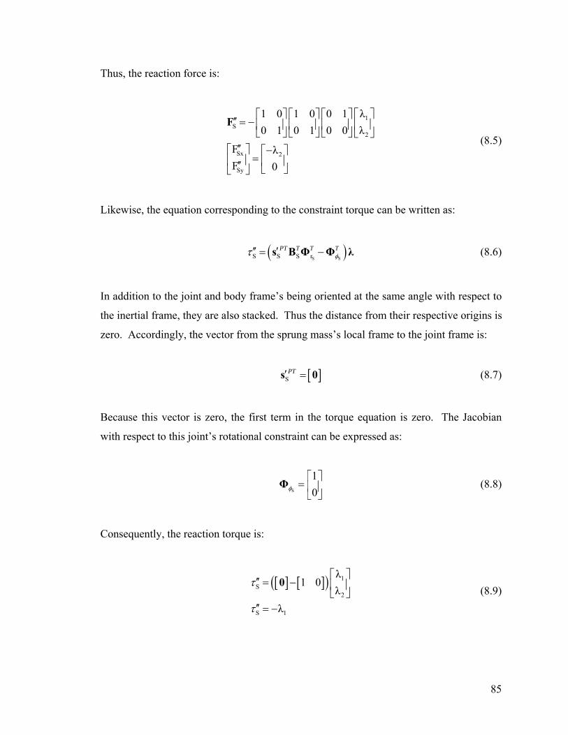
Thus, the reaction force is:

1S

2

Sx 2

Sy

λ1 0 1 0 0 1λ0 1 0 1 0 0

F λF 0

⎡ ⎤⎡ ⎤ ⎡ ⎤ ⎡ ⎤′′ = − ⎢ ⎥⎢ ⎥ ⎢ ⎥ ⎢ ⎥⎣ ⎦ ⎣ ⎦ ⎣ ⎦ ⎣ ⎦

′′⎡ ⎤ −⎡ ⎤=⎢ ⎥ ⎢ ⎥′′ ⎣ ⎦⎣ ⎦

F

(8.5)

Likewise, the equation corresponding to the constraint torque can be written as:

( )S SS S S rPT T T T

φτ ′′ ′= −s B Φ Φ λ (8.6)

In addition to the joint and body frame’s being oriented at the same angle with respect to

the inertial frame, they are also stacked. Thus the distance from their respective origins is

zero. Accordingly, the vector from the sprung mass’s local frame to the joint frame is:

[ ]SPT′ =s 0 (8.7)

Because this vector is zero, the first term in the torque equation is zero. The Jacobian

with respect to this joint’s rotational constraint can be expressed as:

S

10φ⎡ ⎤

= ⎢ ⎥⎣ ⎦

Φ (8.8)

Consequently, the reaction torque is:

[ ] [ ]( ) 1

S2

S 1

λ1 0

λλ

τ

τ

⎡ ⎤′′ = − ⎢ ⎥

⎣ ⎦′′ = −

0 (8.9)

85

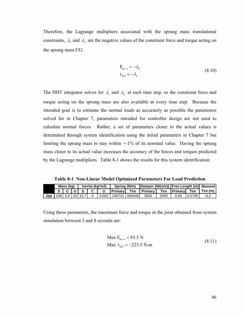
Therefore, the Lagrange multipliers associated with the sprung mass translational

constraints, 1λ and 2λ are the negative values of the constraint force and torque acting on

the sprung mass CG:

Sx 2

S 1

F λτ λ

→ = −= −

(8.10)

The HHT integrator solves for 1λ and 2λ at each time step, so the constraint force and

torque acting on the sprung mass are also available at every time step. Because the

intended goal is to estimate the normal loads as accurately as possible the parameters

solved for in Chapter 7, parameters intended for controller design are not used to

calculate normal forces. Rather, a set of parameters closer to the actual values is

determined through system identification using the initial parameters in Chapter 7 but

limiting the sprung mass to stay within +-1% of its nominal value. Having the sprung

mass closer to its actual value increases the accuracy of the forces and torques predicted

by the Lagrange multipliers. Table 8-1 shows the results for this system identification:

Table 8-1 Non-Linear Model Optimized Parameters For Load Prediction

S C U S C U Primary Tire Primary Tire Primary TireOpt 238 5.6 20 15.7 0 0.002 140731 400048 3500 2000 0.65 0.5795 -0.2

Mass (kg) Inertia (kg*m2) Spring (N/m) Damper {N/(m/s)} Free Length (m) Moment Tire (m)

Using these parameters, the maximum force and torque in the joint obtained from system

simulation between 3 and 8 seconds are:

Sx

S

Max F 93.5 NMax 223.5 N-mτ

→ == −

(8.11)

86

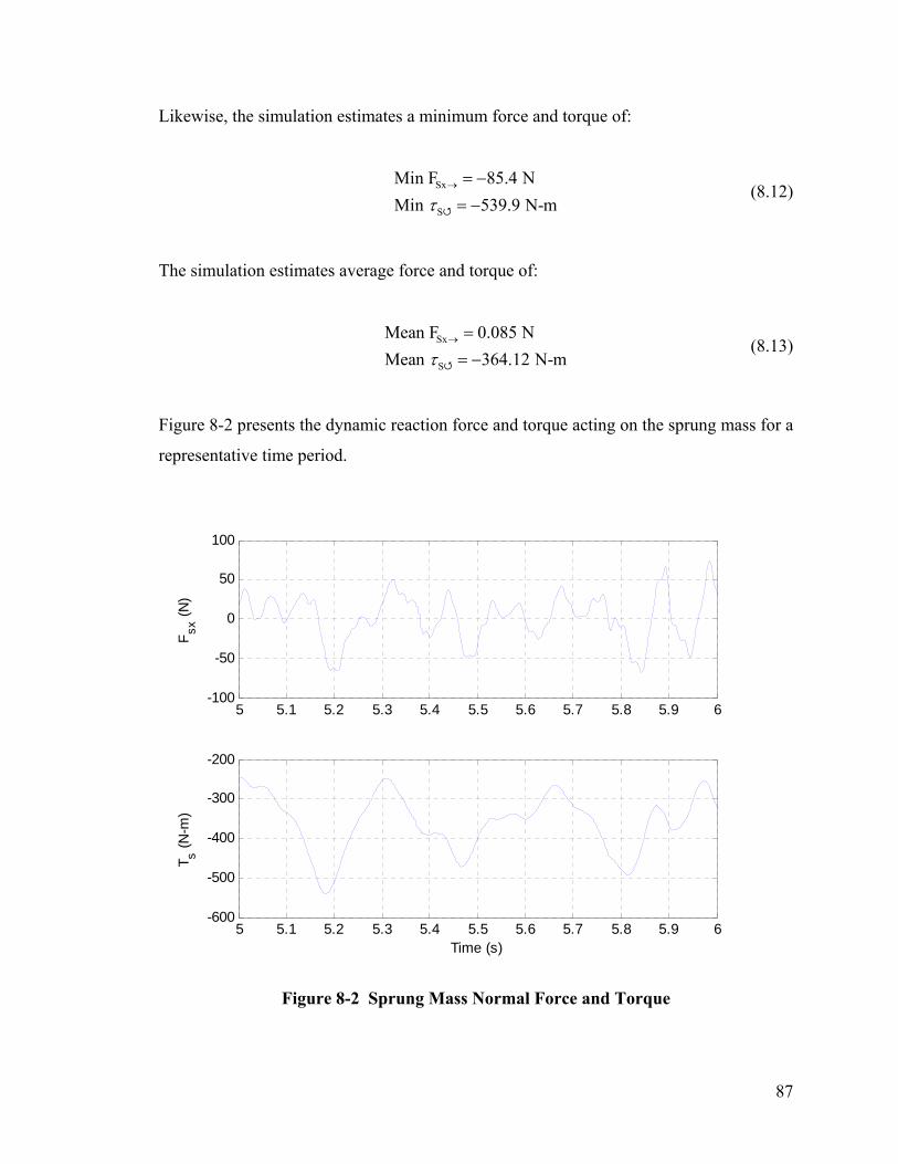
Likewise, the simulation estimates a minimum force and torque of:

Sx

S

Min F 85.4 NMin 539.9 N-mτ

→ = −= −

(8.12)

The simulation estimates average force and torque of:

Sx

S

Mean F 0.085 NMean 364.12 N-mτ

→ == −

(8.13)

Figure 8-2 presents the dynamic reaction force and torque acting on the sprung mass for a

representative time period.

5 5.1 5.2 5.3 5.4 5.5 5.6 5.7 5.8 5.9 6-100

-50

0

50

100

F sx (N

)

5 5.1 5.2 5.3 5.4 5.5 5.6 5.7 5.8 5.9 6-600

-500

-400

-300

-200

T s (N-m

)

Time (s)

Figure 8-2 Sprung Mass Normal Force and Torque

87

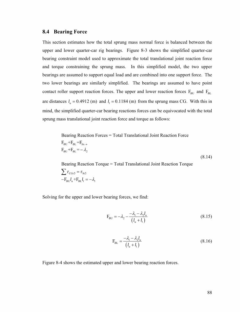
8.4 Bearing Force

This section estimates how the total sprung mass normal force is balanced between the

upper and lower quarter-car rig bearings. Figure 8-3 shows the simplified quarter-car

bearing constraint model used to approximate the total translational joint reaction force

and torque constraining the sprung mass. In this simplified model, the two upper

bearings are assumed to support equal load and are combined into one support force. The

two lower bearings are similarly simplified. The bearings are assumed to have point

contact roller support reaction forces. The upper and lower reaction forces and

are distances and l

BUF BLF

0.4912 (m)ul = 0.1184 (m)l = from the sprung mass CG. With this in

mind, the simplified quarter-car bearing reactions forces can be equivocated with the total

sprung mass translational joint reaction force and torque as follows:

(8.14)

BU BL Sx

BU BL 2

CG S

BU BL 1

Bearing Reaction Forces = Total Translational Joint Reaction ForceF +F =FF +F =

Bearing Reaction Torque = Total Translational Joint Reaction Torque

F +Fu ll l

λ

τ τ

λ

→

−

=

− = −∑

Solving for the upper and lower bearing forces, we find:

( )

1 2BU 2F u

u l

ll lλ λλ − −

= − −+

(8.15)

( )

1 2BLF u

u l

ll lλ λ− −

=+

(8.16)

Figure 8-4 shows the estimated upper and lower bearing reaction forces.

88

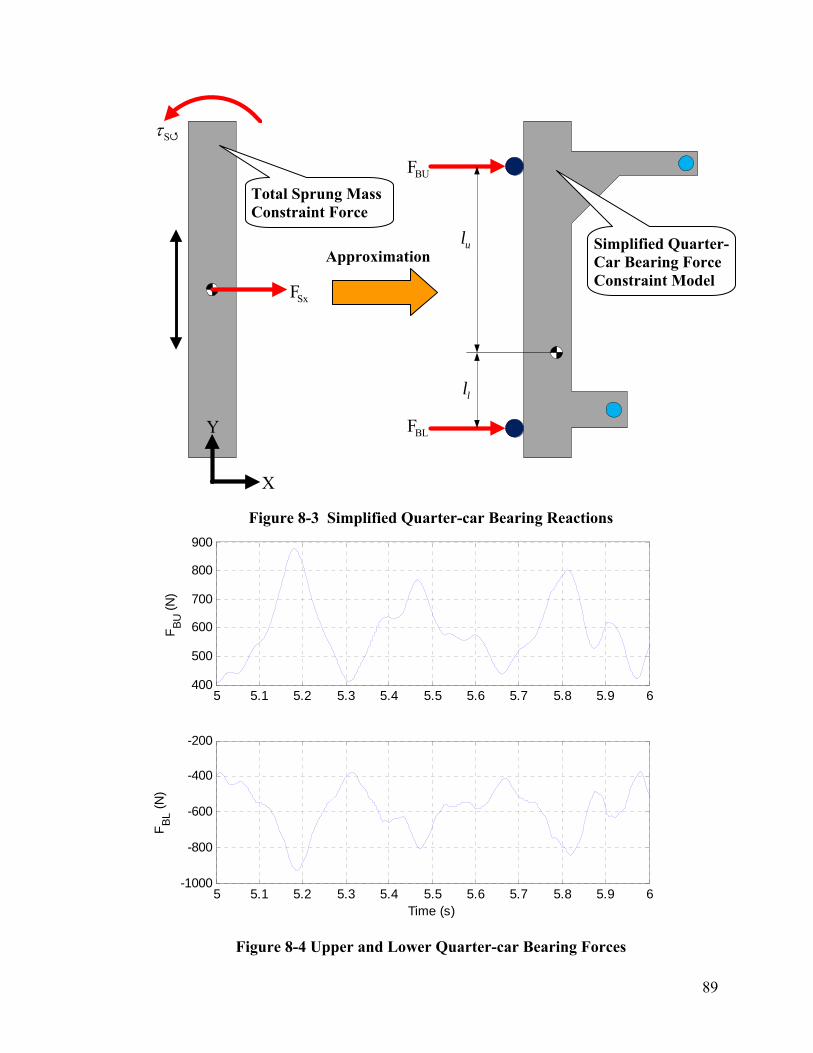
X

Y

SxF

Sτ

BUF

BLF

Total Sprung Mass Constraint Force

Simplified Quarter-Car Bearing Force Constraint Model

ulApproximation

ll

Figure 8-3 Simplified Quarter-car Bearing Reactions

5 5.1 5.2 5.3 5.4 5.5 5.6 5.7 5.8 5.9 6400

500

600

700

800

900

F BU (N

)

5 5.1 5.2 5.3 5.4 5.5 5.6 5.7 5.8 5.9 6-1000

-800

-600

-400

-200

F BL (N

)

Time (s)

Figure 8-4 Upper and Lower Quarter-car Bearing Forces

89

In the context of this thesis, the purpose for obtaining these results is to ensure that the

normal loads applied to the quarter-car rig do not exceed its bearing or structural load

capacity. Before using these results for that purpose, it is advisable to equip the bearings

of the quarter-car rig with either strain gauges or load cells to verify that the simulated

load matches the experimental load. After verification, the simulated reaction forces can

be used with confidence to estimate dynamic normal loads.

Appendix B shows bearing load results with a simplified joint formulation.

90

9. CONCLUSIONS AND RECOMMENDATIONS

This chapter summarizes the results obtained and discusses these results in the context of

the thesis objectives.

9.1 Modeling

The first objective was to formulate linear and non-linear multibody dynamic McPherson

strut suspension models and determine which is more accurate in pursuit of producing

tools to aid controller design. This thesis developed and performed system identification

on linear and non-linear McPherson strut quarter-car models. Using optimal parameters

from their respective system identifications, the non-linear model slightly outperformed

the linear model. Given that the experimental suspension under consideration is

minimally non-linear, the two models’ similarity in performance is expected.

As tools to aid controller design, there is value in both models. Each model is

appropriate for various applications. The linear model may be most appropriate for use

with McPherson strut suspensions that are minimally non-linear such as those found on

race cars and where quick run time is desirable. The non-linear model may be most

appropriate for use with McPherson strut suspensions that are moderately non-linear such

as those found on the majority of small- and medium-sized passenger cars.

9.2 Load Estimation

The second objective was to use the non-linear multibody dynamics model to estimate

the dynamic normal loads applied to the quarter-car rig’s sprung mass plate and bearings.

The non-linear model’s ability to estimate sprung mass normal loads was explored in

Chapter 8 using the translational joint reaction force formula and utilizing Lagrange

multipliers produced by the DAE simulation. The load prediction feature implicit with

the non-linear model can be used to estimate sprung mass normal loads on the quarter-car

rig after validation is performed. Using strain gauges or load cells the experimental load

91

can be measured and compared to the simulated load. After such verification the non-

linear model can be used with confidence for such load estimations.

9.3 Model Template

The third objective was to clearly describe the construction of the multibody dynamics

non-linear model so that it can be used as a template for future use. The goal was to

present the mathematical model in such a way that it could be modified for use with other

McPherson strut configurations. Chapter 6 presents a clear description of how the non-

linear model was developed. Extension of this model to other McPherson strut

suspensions would involve modifying terms of the DAE template provided in Chapter 6.

9.4 Conclusion

This research was successful as the objectives outlined have been met. This research aids

in controller design by providing a mathematical model for McPherson strut suspensions,

and aids in experimental efforts by providing a means to estimate the quarter-car rig’s

sprung mass dynamic normal force. This research also is useful for other McPherson

strut suspension experimentation as well as for experimentation with other suspension

configurations because the model construction is clearly described. It is this author’s

hope that these models will provide functional building blocks for controller design,

future experiments, and general simulation purposes.

9.5 Recommendations for Future Research

Avenues for future research include continued modeling and simulation of the non-linear

model, sprung mass linear bearing load verification, and use of the models for various

applications.

Modeling can be continued in several ways. The primary suspension spring used in the

experimental suspension is actually two springs in series. Modeling this two-element

92

spring as a dual rate spring may improve accuracy. Also, the non-linear kinematic model

was derived as a 2D model because its motions were assumed to be largely planar.

However, a 3D model would account for any caster change or bump steer dynamics, and

therefore has potential to increase the accuracy of this model. However, because the

unsprung mass performance in decibels was approximately half of that achieved by the

sprung mass performance, using a more comprehensive tire model may provide the most

performance gain. More complete tire models, such as the model written about by Gipser

[21], account for various non-linearities exhibited by tires. They also can be formulated

to account for the lateral stiffness of a tire. Representing the tire with such a model has

the potential to increase performance.

Simulation can be continued by choosing joint and CG locations as optimization

parameters. Performance gains may be realized by including these parameters in the

system identification process. By applying these adjustments, the non-linear model’s

accuracy may be improved. However, the benefit of such improvements must be

weighed with any addition to complexity.

In addition to simulation and modeling work the sprung mass linear bearing normal force

predicted by the non-linear model can be verified. By attaching either strain gauges or

load cells inline with the normal load experienced by the linear bearings the normal force

can be experimentally obtained. These results can be compared to the simulated results

in an effort to validate the non-linear model as a sprung mass linear bearing normal force

prediction tool. After verification, the model can be used with confidence for this

purpose.

Future research can be undertaken by using the non-linear model for its myriad of

potential applications. One such application would be to aid active and semi-active

suspensions control algorithm design. Other applications include design of experiments,

general dynamic simulation, and dynamic response prediction. The range of potential

applications is extensive.

93

REFERENCES

[1] T. D. Gillespie, Fundamentals of Vehicle Dynamics: Engineers Inc., 1992. [2] T. Gilles, Automotive Chassis Brakes Steering & Suspension: Thomson Delmar

Learning, 2004. [3] D. A. Mantaras, L. Laque, and C. Vera, "Development and validation of a three-

dimensional kinematic model for the McPherson steering and suspension mechanisms," Mechanism and Machine Theory, vol. 39, pp. 603-619, June, 2004 2004

[4] J. Daniels, Car Suspensions at Work: Theory & Practice of Steering, Handling, & Roadholding: Motor Racing Publications, 1988.

[5] W. F. Milliken and D. L. Milliken, Race Car Vehicle Dynamics: Society of Automotive Engineers Inc., 1995.

[6] J. Garcia de Jalon and E. Bayo, Kinematic and Dynamic Simulation of Multibody systems –The Real-Time Challenge–: Springer, 1993.

[7] E. J. Haug, Computer-Aided Kinematics and Dynamics of Mechanical System volume 1: Basic methods: Allyn and Bacon, 1989.

[8] H. Rahnejat, Multi-Body Dynamics vehicles, Machines, and Mechanisms: Professional Engineering Publishing Limited, 1998.

[9] D. Inman, Engineering Vibration Second Edition: Prentice Hall, 2000. [10] F. D. Goncalves, "Dynamic Analysis of Semi-Active Control Techniques for

Vehicle Applications," in Mechanical Engineering. vol. M.S. Blacksburg: Virginia Polytechnic Institute and State University, 2001.

[11] B. Owren and H. Simonsen, "Alternative integration methods for problems in structural dynamics," Computer Methods in Applied Mechanics and Engineering, vol. 122, pp. 1 – 10, 1995.

[12] O. J. Laurent, "Structure Preservation for Constrained Dynamics with Super Partitioned Additive Runge--Kutta Methods," SIAM Journal on Scientific Computing vol. 20, pp. 416 – 446, 1998 1998.

[13] D. Negrut, G. Ottarson, R. Rampalli, and A. Sajdak, "On an Implementation of the Hilber-Hughes-Taylor Method in the Context of Index 3 Differential-Algebraic Equations of Multibody," Journal of Computational and Nonlinear Dynamics, vol. 2, pp. 73 – 85, 2007.

[14] A. Cardona and M. Geradin, "Time Integration of the Equation of Motion in Mechanical Analysis," Computer and Structures, vol. 33, pp. 801 – 820, 1989.

[15] A. Cardona and M. Geradin, "Numerical Integration of Second Order Differential-Algebraic Systems in Flexible Mechanics Dynamics," in Computer-Aided Analysis of Rigid and Flexible Mechanical Systems NATO ASI Series E: Applied Sciences, Edited by Pereira, Manuel F.O. Seabra and Ambrosio, Jorge. vol. 268 Kluwer Academic Publishers, 1994, pp. 501-529.

[16] R. L. Burden and J. D. Fares, Numerical Analysis 8th Edition: Thomas Brooks/Cole, 2005.

[17] J. D. Trom, J. L. Lopez, and M. J. Vanderpeg, "Modeling of a Mid-size Passenger Car Using a Multibody Dynamics Program," Journal of Mechanisms Transmissions, and Automation in Design, vol. 109, pp. 518-523, 1987.

94

[18] J. Park, D. A. Guenther, and G. J. Heydinger, "Kinematic Suspension Model Applicable to Dynamic Full Vehicle Simulation," SAE Technical Paper Series No 2003-01-0859, 2003.

[19] M. K. Salaani, G. J. Heydinger, and P. A. Grygier, "Parameter Determination and Vehicle Dynamics Modeling For the NADS of the 1998 Chevrolet Malibu For the National Advanced Driving Simulator," SAE Technical Paper Series No 2001-01-0140, 2001.

[20] B. Ozdalyan, M. V. Blundell, and B. Phillips, "Comparison of suspension rig measurements with computer simulation," in Simulation '98. International Conference, 1998, pp. 133 – 139.

[21] M. Gipser, "FTire: a physically based application-oriented tyre model for use with detailed MBS and finite-element suspension models," Vehicle System Dynamics, vol. 43, pp. 76-91, 2005.

95

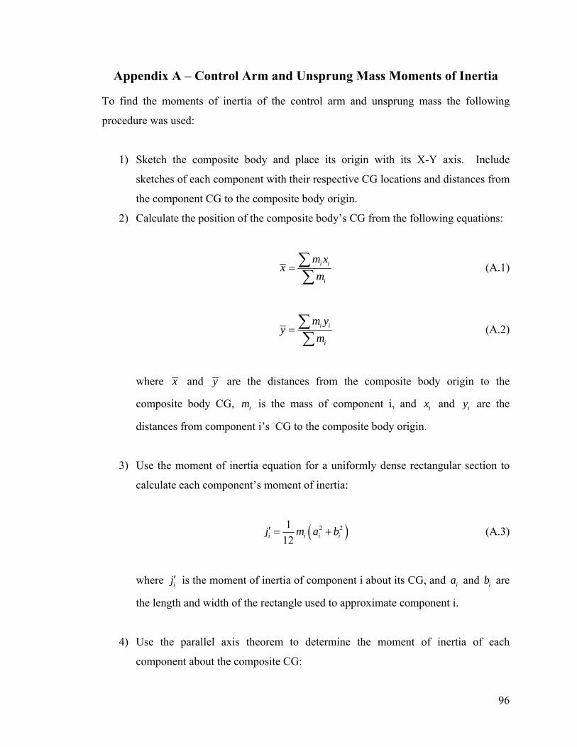
Appendix A – Control Arm and Unsprung Mass Moments of Inertia

To find the moments of inertia of the control arm and unsprung mass the following

procedure was used:

1) Sketch the composite body and place its origin with its X-Y axis. Include

sketches of each component with their respective CG locations and distances from

the component CG to the composite body origin.

2) Calculate the position of the composite body’s CG from the following equations:

i i

i

m xx

m= ∑∑

(A.1)

i i

i

m yy

m= ∑∑

(A.2)

where x and y are the distances from the composite body origin to the

composite body CG, is the mass of component i, and im ix and iy are the

distances from component i’s CG to the composite body origin.

3) Use the moment of inertia equation for a uniformly dense rectangular section to

calculate each component’s moment of inertia:

( 2 2112i i i )ij m a b′ = + (A.3)

where ij′ is the moment of inertia of component i about its CG, and and are

the length and width of the rectangle used to approximate component i.

ia ib

4) Use the parallel axis theorem to determine the moment of inertia of each

component about the composite CG:

96

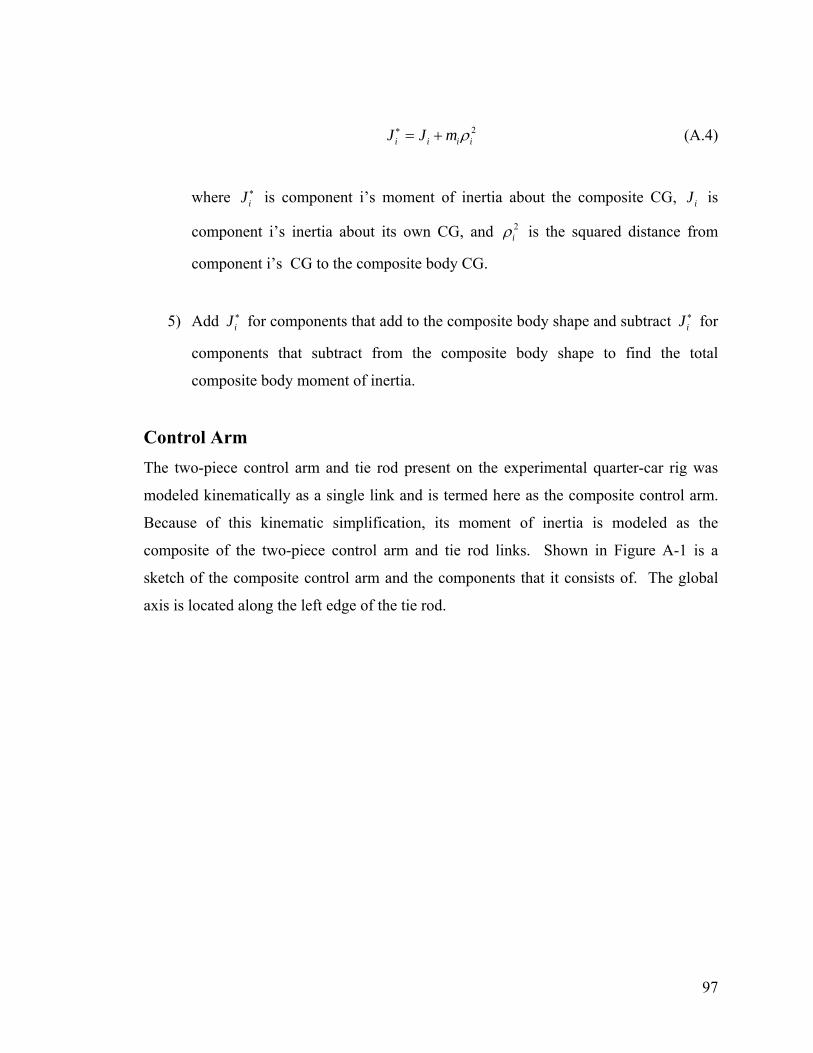
2i i iJ J m iρ∗ = + (A.4)

where is component i’s moment of inertia about the composite CG, is

component i’s inertia about its own CG, and

iJ ∗iJ

2iρ is the squared distance from

component i’s CG to the composite body CG.

5) Add iJ ∗ for components that add to the composite body shape and subtract iJ ∗ for

components that subtract from the composite body shape to find the total

composite body moment of inertia.

Control Arm The two-piece control arm and tie rod present on the experimental quarter-car rig was

modeled kinematically as a single link and is termed here as the composite control arm.

Because of this kinematic simplification, its moment of inertia is modeled as the

composite of the two-piece control arm and tie rod links. Shown in Figure A-1 is a

sketch of the composite control arm and the components that it consists of. The global

axis is located along the left edge of the tie rod.

97

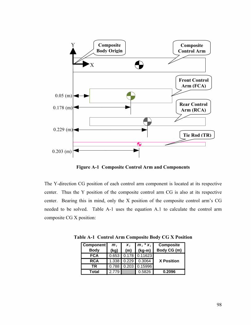
X

Y Composite Body Origin

Composite Control Arm

Front Control Arm (FCA)

0.05 (m)

Rear Control Arm (RCA)0.178 (m)

0.229 (m)Tie Rod (TR)

0.203 (m)

Figure A-1 Composite Control Arm and Components

The Y-direction CG position of each control arm component is located at its respective

center. Thus the Y position of the composite control arm CG is also at its respective

center. Bearing this in mind, only the X position of the composite control arm’s CG

needed to be solved. Table A-1 uses the equation A.1 to calculate the control arm

composite CG X position:

Table A-1 Control Arm Composite Body CG X Position

FCA 0.653 0.178 0.11623RCA 1.338 0.229 0.3064TR 0.788 0.203 0.15996

Total 2.779 0.5826 0.2096

X Position

Component Body

m i

(kg)x i

(m)m i * x i

(kg-m)Composite

Body CG (m)

98

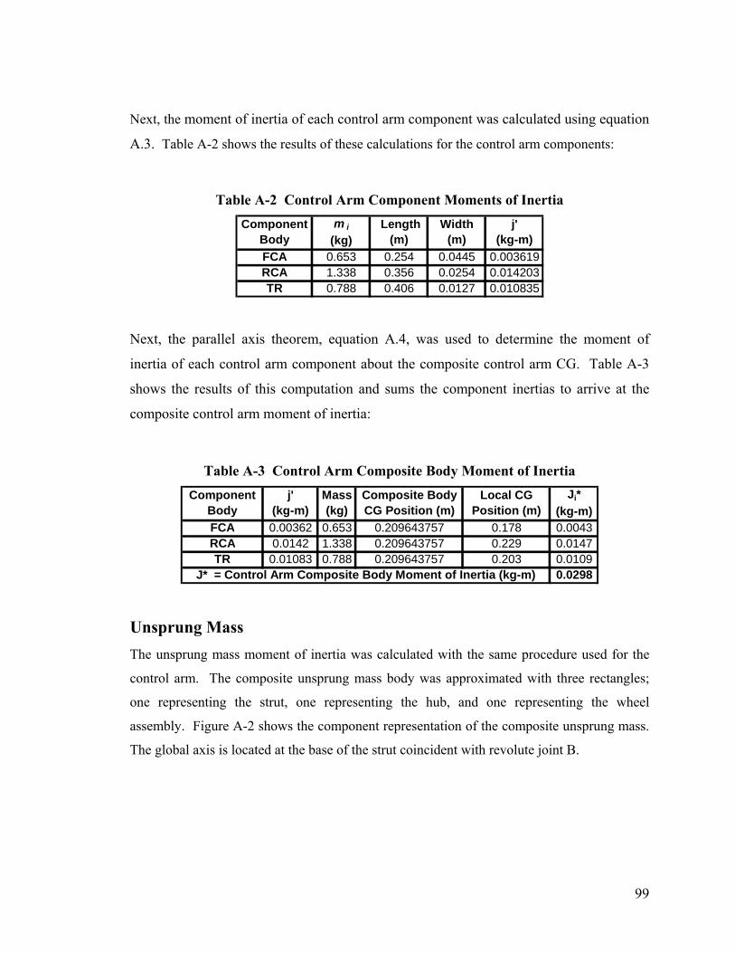
Next, the moment of inertia of each control arm component was calculated using equation

A.3. Table A-2 shows the results of these calculations for the control arm components:

Table A-2 Control Arm Component Moments of Inertia

FCA 0.653 0.254 0.0445 0.003619RCA 1.338 0.356 0.0254 0.014203TR 0.788 0.406 0.0127 0.010835

Component Body

j' (kg-m)

Width (m)

Length (m)

m i

(kg)

Next, the parallel axis theorem, equation A.4, was used to determine the moment of

inertia of each control arm component about the composite control arm CG. Table A-3

shows the results of this computation and sums the component inertias to arrive at the

composite control arm moment of inertia:

Table A-3 Control Arm Composite Body Moment of Inertia

FCA 0.00362 0.653 0.209643757 0.178 0.0043RCA 0.0142 1.338 0.209643757 0.229 0.0147TR 0.01083 0.788 0.209643757 0.203 0.0109

0.0298J* = Control Arm Composite Body Moment of Inertia (kg-m)

Ji* (kg-m)

Local CG Position (m)

Composite Body CG Position (m)

Mass (kg)

j' (kg-m)

Component Body

Unsprung Mass The unsprung mass moment of inertia was calculated with the same procedure used for the

control arm. The composite unsprung mass body was approximated with three rectangles;

one representing the strut, one representing the hub, and one representing the wheel

assembly. Figure A-2 shows the component representation of the composite unsprung mass.

The global axis is located at the base of the strut coincident with revolute joint B.

99

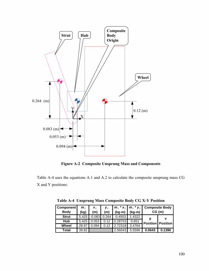
0.12 (m)Y

X

Composite Body Origin

Strut Hub

Wheel

0.264 (m)

0.083 (m)

0.053 (m)

0.094 (m)

Figure A-2 Composite Unsprung Mass and Components

Table A-4 uses the equations A.1 and A.2 to calculate the composite unsprung mass CG

X and Y positions:

Table A-4 Unsprung Mass Composite Body CG X-Y Position

Strut 5.425 -0.083 0.264 -0.4503 1.4322Hub 5.425 0.053 0.12 0.28753 0.651

Wheel 28.97 0.094 0.12 2.72318 3.4764Total 39.82 2.56043 5.5596 0.0643 0.1396

y i

(m)m i * x i

(kg-m)m i * y i

(kg-m)Composite Body

CG (m)

Y Position

X Position

m i

(kg)Component

Bodyx i

(m)

100

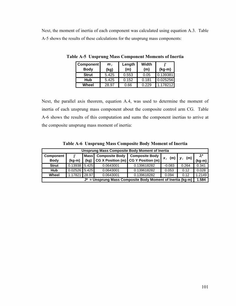
Next, the moment of inertia of each component was calculated using equation A.3. Table

A-5 shows the results of these calculations for the unsprung mass components:

Table A-5 Unsprung Mass Component Moments of Inertia

Strut 5.425 0.553 0.05 0.139381Hub 5.425 0.152 0.181 0.025256

Wheel 28.97 0.66 0.229 1.178212

Component Body

j' (kg-m)

Width (m)

Length (m)

m i

(kg)

Next, the parallel axis theorem, equation A.4, was used to determine the moment of

inertia of each unsprung mass component about the composite control arm CG. Table

A-6 shows the results of this computation and sums the component inertias to arrive at

the composite unsprung mass moment of inertia:

Table A-6 Unsprung Mass Composite Body Moment of Inertia

Strut 0.13938 5.425 0.0643001 0.139618282 -0.083 0.264 0.341Hub 0.02526 5.425 0.0643001 0.139618282 0.053 0.12 0.028

Wheel 1.17821 28.97 0.0643001 0.139618282 0.094 0.12 1.21491.584

y i (m)

J* = Unsprung Mass Composite Body Moment of Inertia (kg-m)

Unsprung Mass Composite Body Moment of InertiaJi*

(kg-m)x i (m)Composite Body

CG X Position (m)Mass (kg)

j' (kg-m)

Component Body

Composite Body CG Y Position (m)

101

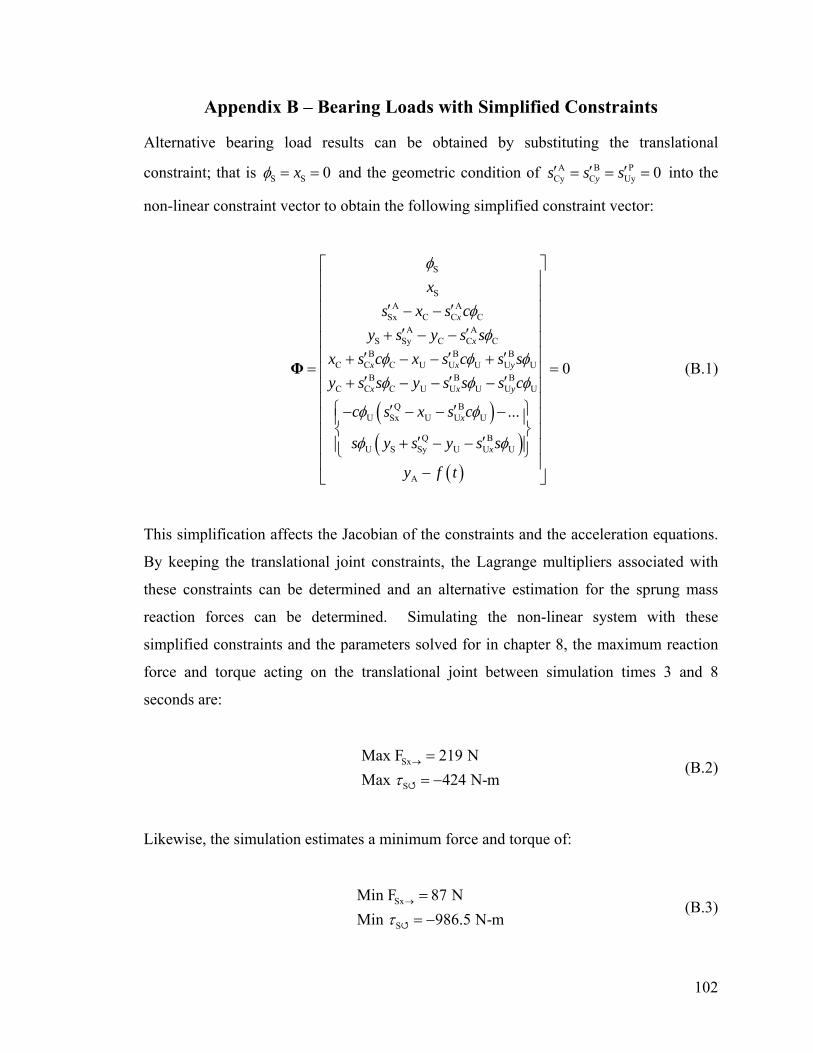
Appendix B – Bearing Loads with Simplified Constraints

Alternative bearing load results can be obtained by substituting the translational

constraint; that is S S 0xφ = = and the geometric condition of into the

non-linear constraint vector to obtain the following simplified constraint vector:

A B PCy C Uy 0ys s s′ ′ ′= = =

( )( )

( )

S

SA A

Sx C C CA A

S Sy C C CB B B

C C C U U U U UB B B

C C C U U U U U

Q BU Sx U U U

Q BU S Sy U U U

A

...

x

x

x x y

x x y

x

x

xs x s c

y s y s sx s c x s c s sy s s y s s s c

c s x s c

s y s y s s

y f t

φ

φφ

φ φ φφ φ φ

φ φ

φ φ

⎡ ⎤⎢ ⎥⎢ ⎥

′ ′⎢ ⎥− −⎢ ⎥′ ′+ − −⎢ ⎥⎢ ⎥′ ′ ′+ − − += ⎢

′ ′ ′+ − − −⎢ ⎥⎢ ⎥⎧ ⎫′ ′− − − −⎢ ⎥⎪ ⎪⎨ ⎬⎢ ⎥′ ′+ − −⎪ ⎪⎢ ⎩ ⎭

⎢ −⎣ ⎦

Φ 0⎥ =

⎥⎥

(B.1)

This simplification affects the Jacobian of the constraints and the acceleration equations.

By keeping the translational joint constraints, the Lagrange multipliers associated with

these constraints can be determined and an alternative estimation for the sprung mass

reaction forces can be determined. Simulating the non-linear system with these

simplified constraints and the parameters solved for in chapter 8, the maximum reaction

force and torque acting on the translational joint between simulation times 3 and 8

seconds are:

Sx

S

Max F 219 NMax 424 N-mτ

→ == −

(B.2)

Likewise, the simulation estimates a minimum force and torque of:

Sx

S

Min F 87 NMin 986.5 N-mτ

→ == −

(B.3)

102

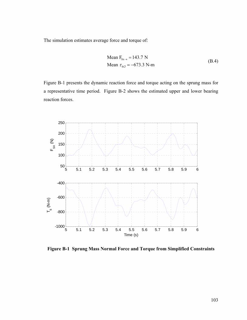
The simulation estimates average force and torque of:

Sx

S

Mean F 143.7 NMean 673.3 N-mτ

→ == −

(B.4)

Figure B-1 presents the dynamic reaction force and torque acting on the sprung mass for

a representative time period. Figure B-2 shows the estimated upper and lower bearing

reaction forces.

5 5.1 5.2 5.3 5.4 5.5 5.6 5.7 5.8 5.9 650

100

150

200

250

F sx (N

)

5 5.1 5.2 5.3 5.4 5.5 5.6 5.7 5.8 5.9 6-1000

-800

-600

-400

T s (N-m

)

Time (s)

Figure B-1 Sprung Mass Normal Force and Torque from Simplified Constraints

103

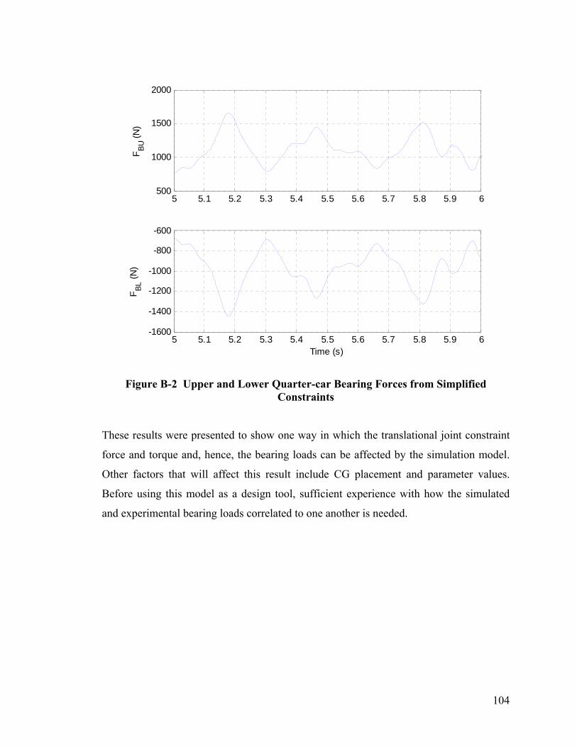
5 5.1 5.2 5.3 5.4 5.5 5.6 5.7 5.8 5.9 6500

1000

1500

2000

F BU (N

)

5 5.1 5.2 5.3 5.4 5.5 5.6 5.7 5.8 5.9 6-1600

-1400

-1200

-1000

-800

-600

F BL (N

)

Time (s)

Figure B-2 Upper and Lower Quarter-car Bearing Forces from Simplified Constraints

These results were presented to show one way in which the translational joint constraint

force and torque and, hence, the bearing loads can be affected by the simulation model.

Other factors that will affect this result include CG placement and parameter values.

Before using this model as a design tool, sufficient experience with how the simulated

and experimental bearing loads correlated to one another is needed.

104

Multibody Dynamics Modeling and System Identification for ...

Documents

Transcript of Multibody Dynamics Modeling and System Identification for ...