Multi-View Self-Paced Learning for ClusteringChang Xu† Dacheng Tao‡ Chao Xu†

†Key Lab. of Machine Perception (Ministry of Education)Peking University, Beijing 100871, China

‡Centre for Quantum Computation and Intelligent SystemsUniversity of Technology, Sydney 2007, Australia

xuchang@pku.edu.cn dacheng.tao@uts.edu.au xuchao@cis.pku.edu.cn

AbstractExploiting the information from multiple views canimprove clustering accuracy. However, most ex-isting multi-view clustering algorithms are non-convex and are thus prone to becoming stuck intobad local minima, especially when there are out-liers and missing data. To overcome this prob-lem, we present a new multi-view self-paced learn-ing (MSPL) algorithm for clustering, that learnsthe multi-view model by not only progressing from‘easy’ to ‘complex’ examples, but also from ‘easy’to ‘complex’ views. Instead of binarily separatingthe examples or views into ‘easy’ and ‘complex’,we design a novel probabilistic smoothed weight-ing scheme. Employing multiple views for cluster-ing and defining complexity across both examplesand views are shown theoretically to be beneficialto optimal clustering. Experimental results on toyand real-world data demonstrate the efficacy of theproposed algorithm.

1 IntroductionData collected from diverse sources or extracted from differ-ent feature extractors have heterogeneous features in manyreal-world applications [Xu et al., 2013]. For example, whenclassifying webpages, a webpage can be described by its con-tent, the text of webpages linking to it, and the link struc-ture of linked pages [Xu et al., 2014]. Several differentdescriptors have been proposed to enhance action recogni-tion performance, each of which describes certain aspectsof object action [Xu et al., 2015]. In particular, histogramsof oriented gradients (HOG) [Dalal and Triggs, 2005] focuson static appearance information, histograms of optical flow(HOF) [Laptev et al., 2008] capture absolute motion infor-mation, and motion boundary histograms (MBH) [Dalal etal., 2006] encode related motion between pixels. Since theseheterogeneous features have distinct physical meanings andrepresent objects from different perspectives, they can natu-rally be regarded as multiple data views [Nguyen et al., 2013;Xie and Xing, 2013].

Clustering aims to find meaningful groups of examples inan unsupervised manner for exploratory data analysis. In-dependently employing each view makes clustering inaccu-

rate, since each individual view does not comprehensivelydescribe all the examples. Therefore, it is beneficial to usemultiple views and exploit their connections to improve clus-tering. This approach has given the rise to the field of multi-view clustering.

A number of promising multi-view clustering algorithmshave been developed. [de Sa, 2005; Zhou and Burges, 2007;Kumar et al., 2011a] fuse similarity measurements from di-verse views to construct a graph for multi-view examples,which successfully extends conventional single-view spectralclustering methods to the multi-view setting. [Chaudhuri etal., 2009; Liu et al., 2013; Cai et al., 2013] project multi-ple views into a shared latent subspace, in which the conven-tional single-view clustering algorithms can then be used todiscover clusters.

Most existing multi-view clustering methods aim to solvenon-convex objective functions. These can result in the solu-tions stuck in bad local minima, especially in the presence ofnoise and outliers. A heuristic method to alleviate this prob-lem is to launch the algorithm multiple times with differentinitializations and then choose the best solution. However,this strategy is time consuming and generally difficult to im-plement in the unsupervised setting, since there is no explicitcriterion for model selection.

By simulating human learning, self-paced learning [Kumaret al., 2010] first attempts to train a model on ‘easy’ examplesand then gradually take ‘complex’ examples into considera-tion. This has been shown to be beneficial in avoiding badlocal minima and improving the generalization result [Kumaret al., 2011b; Tang et al., 2012; Zhao et al., 2015]. As well asthe complexities of examples in each individual view, multi-view examples might also have ‘easy’ and ‘complex’ views,and the distinction between ‘easy’ and ‘complex’ views mightbe different for distinct multi-view examples. For example,GIST features [Oliva and Torralba, 2001] achieve high ac-curacy when used to recognize natural scene images, whileCENTRIST features [Wu and Rehg, 2008] are good at classi-fying indoor environment images.

In this paper, we propose Multi-view Self-Paced Learning(MSPL) for clustering, which learns multi-view models byconsidering the complexities of both examples and views. In-stead of hard treating examples or views as ‘easy’ or ‘com-plex’, we design a smoothed weighting scheme that inher-its the merits of logistic function and provides probabilistic

Proceedings of the Twenty-Fourth International Joint Conference on Artificial Intelligence (IJCAI 2015)

3974

weights. The resulting objective function is solved by a sim-ple yet effective method. Using multiple views for cluster-ing and the easy-to-complex strategy are proven theoreticallyto be beneficial for approximating the ideal clustering result.Experimental results on toy and real-world data demonstratethe effectiveness of the algorithm in distinguishing complex-ities across examples and views to improve clustering perfor-mance.

2 Problem FormulationAs a classical algorithm, k-means clustering uses k prototypevectors (i.e., centers or centroids of k clusters) to character-ize the data and minimize a sum of squared loss function tofind these prototypes using a coordinate descent optimizationmethod. It has been shown that non-negative matrix factor-ization is equivalent to relaxed k-means [Ding et al., 2005].Given n examples X = [x1, · · · , xn] ∈ RD×n, the k-meansclustering objective can be reformulated as

minB,C

‖X − CB‖2F

s.t. Bij ∈ {0, 1},k∑i

Bij = 1,∀j ∈ [1, n](1)

where C = [c1, · · · , ck] ∈ RD×k is the centroid matrixwith ci as the cluster centroid of the i-th cluster, and B =[b1, · · · , bn] ∈ Rk×n denotes clustering assignment. If the j-th example is assigned to the i-th cluster, Bij = 1; otherwiseBij = 0.

The original k-means clustering method only works forsingle-view data. The obvious route to adapting single-viewclustering algorithms to the multi-view setting is to concate-nate the features of multiple views into a long feature vector.Since multiple views have distinct physical meanings and de-scribe the objects from different perspectives, treating theseviews equally without in-depth analysis usually fails to pro-duce the optimal result. Therefore, it is necessary to exploitthe connections between multiple views to improve clusteringperformance.

2.1 Multi-view Self-Paced LearningLet Xv ∈ RDv×n and Cv ∈ RDv×k denote the features andcentroid matrix of the v-th view, respectively. In multi-viewclustering, the clustering results of different views should beconsistent; that is, given different centroid matrices, the clus-tering assignments of m views should be the same. Hence,Eq. (1) can be extended to handle multi-view examples:

minB,C

m∑v=1

‖Xv − CvB‖2F

s.t. Bij ∈ {0, 1},k∑i

Bij = 1,∀j ∈ [1, n],

(2)

where B is the assignment matrix shared by m views.Neither the single-view formulation Eq. (1) nor the multi-

view formulation Eq. (2) is a convex problem, and thus theyboth have the risk of getting stuck in bad local minima during

optimization. Recently, self-paced learning has been used toalleviate this problem. The general self-paced learning modelis composed of a weighted loss term on all examples and aregularizer term imposed on example weights. By graduallyincreasing the penalty on the regularizer during model opti-mization, more examples are automatically included in train-ing from ‘easy’ to ‘complex’ via a pure self-paced approach.The distinction between ‘easy’ and ‘complex’ not only existsacross examples but also across views. Since multiple viewshave distinct physical meanings and describe examples fromdifferent perspectives, a multi-view example can naturally bemore easily distinguished in one view than in the other views.By simultaneously considering the complexities of both ex-amples and views, we develop multi-view self-paced learningfor clustering:

minW,B,C

m∑v=1

‖(Xv − CvB)diag(√wv)‖2F + f(W )

s.t. Bij ∈ {0, 1},k∑i

Bij = 1,∀j ∈ [1, n],

wv ∈ [0, 1]n,∀v ∈ [1,m],

(3)

where wv = [wv1 , · · · , wvn] is composed of the weights of nexamples in the v-th view, W = [w1; · · · ;wm], and f(W )denotes the regularizer determining the examples and viewsto be selected during training. The previously adopted f(W )in [Kumar et al., 2010] was simply

f(W ) = − 1

λ

m∑v=1

n∑i=1

wvi, (4)

which indicates that the optimal weight for the i-th examplein the v-th view is

w∗vi =

1 if `vi ≤

1

λ,

0 if `vi >1

λ,

(5)

where `vi stands for the reconstruction error of the i-th ex-ample in the v-th view. Taking 1

λ as the threshold, ‘easy’examples (views) have losses less than the threshold, whilethe losses of ‘complex’ examples (views) are greater than thethreshold. The parameter λ controls the pace at which themodel learns new examples (views), and it is usually itera-tively decreased during optimization.

Note that the classical regularizer (i.e., Eq. (4)) hard selectsexamples (views) by assigning them binary weights, as shownin Figure 1. Since noise is usually non-homogeneously dis-tributed in the data, it is unreasonable to absolutely assert thatone example (view) is easy or complex. As demonstratedin many real-world applications, soft weighting is more ef-fective than the hard weighting and can faithfully reflect thetrue importance of examples (views) during training. Hence,instead of hard weighting, we propose a new regularizer forself-paced learning:

f(wvi) = ln(1 + e−1λ − wvi)(1+e

− 1λ−wvi)

+ ln(wvi)wvi − wvi

λ.

(6)

3975

0 2 4 6 8 10 12 14 150

0.2

0.4

0.6

0.8

1

Loss

Wei

ght

data25data26data27data28data29data30data31data32data33data34data35data36data37data38data39data40data41data42data43data44data45data46h=1h=0.5h=0.2h=0.125

Figure 1: Comparison of the regularizers for self-paced learn-ing. Solid curves correspond to smoothed weighting (i.e., Eq.(8)), while dashed curves correspond to hard weighting (i.e.,Eq. (5)).

The optimal weight of the i-th example in the v-th view canbe solved using

minwvi∈[0,1]

wvi`vi + f(wvi) (7)

by setting the gradient with respect to wvi to zero,

w∗vi =1 + e−

1λ

1 + e`vi−1λ

. (8)

Compared to Eq. (5), Eq. (8) is a smoothed function re-lated to `vi, and its function curves under different λ’s arepresented in Figure 1. It is instructive to note that function(8) can be regarded as an adapted logistic function, whichis a well-known loss function in machine learning. Hence,Eq. (8) can inherit all the merits of logistic function, whichis infinitely many times differentiable, strictly convex, andLipschitz continuous. Most importantly, Eq. (8) provides aprobabilistic interpretation of the weights, because given dif-ferent inputs it always outputs values between zero and one.Instead of hard separating the examples and views into ‘easy’and ‘complex’ as in Eq. (5), Eq. (8) tends to assign examplesand views the probabilities of being ‘easy’. Different from 1

λ

in Eq. (5), which determines whether w∗vi = 1 or w∗vi = 0 , 1λ

in Eq. (8) influences the speed of change of the weight withregard to the loss. It can be seen that when the loss is less than1λ , the examples and views can be implicitly treated as ‘easy’since as their weights vary slowly with respect to the corre-sponding loss; otherwise, they are ‘complex’ in line with thefast variation of the weight with respect to the loss. Further-more, as 1

λ increase, more examples and views are likely tobe included to train a mature model.

By combining Eqs. (3) and (6), we obtain the resulting ob-jective function. In optimizing the proposed model, we prob-abilistically measure the complexity of examples and viewsand then gradually train the multi-view clustering model from‘easy’ to ‘complex’ to prevent falling into bad local minima.

3 OptimizationWe solve the optimization problem in an alternating fashion.Under fixed centroid matrices {Cv}mv=1and assignment ma-

trix B, W can be optimized by

minW

m∑v=1

‖(Xv − CvB)diag(√wv)‖2F + f(W ). (9)

By adopting the regularizer f(W ) as in Eq. (6), we find thatthe optimal W can naturally satisfy the constraint that wv ∈[0, 1]n,∀v ∈ [1,m]. According to the discussion in Section2.1, the optimal solution W ∗ can be written out in a closedform as in Eq. (8).

If we focus on centroid matrixCv in the v-th view and keepthe other centroid matrices, assignment matrix, and weightmatrix fixed, we obtain the following sub-problem:

minCvJ = ‖(Xv − CvB)W v‖2F , (10)

where W v = diag(√wv). Taking the derivative of J with

respect to Cv , we obtain

∂J∂Cv

= 2(Xv − CvB)W v(W v)TBT . (11)

Setting Eq. (11) as zero, we can update Cv through

Cv = (XvW v(W v)TBT )(B(W v)TBT )−1. (12)

When we fix all the centroid matrices on different viewsand the weights, the original problem is reduced to

minB

m∑v=1

‖(Xv − CvB)W v‖2F

s.t. Bij ∈ {0, 1},k∑i

Bij = 1,∀j ∈ [1, n].

(13)

Since each entry of B is a binary integer and each columnvector must only have a non-zero entry, it is difficult to opti-mize matrix B as a whole. We solve this problem by decou-pling the data and assigning the cluster centroid for them se-quentially and independently. For the i-th example, we needto solve

minbi

m∑v=1

wvi‖xvi − Cvbi‖22

s.t. bi ∈ {0, 1}k, ‖bi‖1 = 1,

(14)

where bi is the i-th column vector of matrix B and recordsthe clustering assignment of the i-th example. Given the factthat there are k candidates as the solution of Eq. (14), eachof which is the column of matrix Ik = [e1, · · · , ek], we canperform an exhaustive search to obtain the solution of Eq.(14) as b∗i = ej , where j is decided as:

j = arg minj

m∑v=1

wvi‖xvi − Cvej‖22 (15)

Given the above optimization scheme over each objectivevariable, we alternatively update {Cv}mv=1, B, and W andrepeat the process iteratively until the objective function con-verges.

3976

4 Theoretical AnalysisIn this section, we analyze the advantages of multi-view clus-tering and the influence of self-paced learning on clusteringperformance. Since the weights of all examples and viewswill eventually be assigned 1’s during training, we first ana-lyze the resulting clustering performance without weights forsimplicity, and then discuss the influence of self-paced learn-ing on training.

Starting from Eq. (1), it is easy to note that the clus-ters’ centroids are given by the averaged vectors of examplesfalling into them. The rows ofB are mutually orthogonal vec-tors. We normalize these row vectors to length 1 and denotethe new matrix B. The distortion of multi-view clustering canthus be written as

D(B) =m∑v=1

(tr((Xv)TXv

)− tr(B(Xv)TXvBT

)). (16)

Since the last cluster can be determined by the other (k − 1)

clusters, we can uniquely represent B by matrix Y with (k−1) orthogonal rows,

V B =[Y ; 1

1√n

], (17)

where V is a k × k orthogonal matrix with its last row asv−1 = [

√n1

n , · · · ,√

nkn ], and 1 denotes the row vector of all

1’s. D(B) can thus be reformulated in terms of Y

D(Y ) =m∑v=1

(tr((Xv)TXv

)− tr(Y (Xv)TXvY T

)), (18)

where we assume that the input data are centered at the origin,i.e.,Xv1T = 0. According to [Ding and He, 2004], the lowerbound of D(Y ) is

m∑v=1

(tr((Xv)TXv

)−k−1∑i=1

σvi

)= D∗ ≤ D(Y ), (19)

where σv1 , · · · , σvk are the top (k−1) principal eigenvalues of(Xv)TXv .

We first attempt to bound the difference betweenD(Y ) andD∗. Assume that Uvt ∈ R(k−1)×n and Uvr ∈ R(n−k+1)×n arecomposed of the top (k − 1) principal eigenvectors and theremaining (n − k + 1) principal eigenvectors of (Xv)TXv

in the v-the view, respectively. [Uvt ;Uvr ] can be regarded asthe orthogonal basis in the v-th view in space Rn. Y canthus be represented by the bases in different views in distinctformulations:

Y =[E1t E

1r

] [U1t

U1r

]; · · · ;Y = [Emt Emr ]

[UmtUmr

], (20)

where Evt ∈ R(k−1)×(k−1) and Evr ∈ R(k−1)×(n−k+1) arethe coefficients corresponding to Uvt and Uvr in the v-th view,respectively. To better represent the dataset using k clusters,Y should be constructed using the top (k−1) principal eigen-vectors in each view as much as possible; that is, the smaller{‖Evr ‖F }mv=1, the better the clustering. The following lemmaprovides a bound on {Evr }mv=1.

Lemma 1. By factorizing the clustering Y in the v-th view,we have

‖Evr ‖2F ≤ δv =Dv(Y )−D∗vσvk−1 − σvk

. (21)

Proof. Denoting Dv(Y ) and D∗v as the real and ideal distor-tion in the v-th view, respectively, we have

Dv(Y )−D∗v = tr(Σv

t )−tr(Evt Σv

t (Evt )T )−tr(Ev

r Σvr(Ev

r )T ), (22)

where Σvt = diag(σv1 , · · · , σvk−1) and Σvr =diag(σvk , · · · , σvn). Given α ∈ (σvk−1, σ

vk), we have

tr(Σvt ) ≥ tr(Evt Σvt (Evt )T ) + αtr(Evr (Evr )T ), (23)

and Eq. (22) can be relaxed to

Dv(Y )−D∗v ≥tr(Evr (αI − Σvr)(E

vr )T)

≥tr(Evr (αI − σvkI)(Evr )T

)=(α− σvk)‖Evr ‖2F .

(24)

When α approaches σvk−1, we obtain

Dv(Y )−D∗v ≥ (σvk−1 − σvk)‖Evr ‖2F . (25)

Given σvk−1 − σvk 6= 0, we obtain the desired result.

In general, D∗ cannot be achieved since it is usually im-possible to make Y simultaneously consistent with the sub-spaces spanned by the top (k − 1) principal eigenvectors of{(Xv)TXv}mv=1 in multiple views. Denoting Y opt as theclustering in multiple views with the smallest distortion, wethen note that D∗ ≤ D(Y opt) ≤ D(Y ). Given two cluster-ings B and B

′, it is easy to show that the confusion matrix is

M = B(B′)T . For a stable evaluation of clustering perfor-

mance, the misclassification error (see e.g., [Meila, 2012]) iscomputed by

ME(B, B′) = 1− Purity(B, B

′), (26)

whose connection with φ(B, B′) = ‖B(B

′)T ‖2F is estab-

lished in [Meila, 2012]. The difference between B and Boptcan be bounded by the following theorem.

Theorem 1. Let B be the multi-view clustering result. Givenpmin = mini ni/n and pmax = maxi ni/n, if δv ≤ k−1

2 andminv ε(δv) ≤ pmin, we have

ME(B, Bopt) ≤ pmax minvε(δv),

where

ε(δv) = 2δv(1−δv

k − 1). (27)

Proof. Starting with Eq. (17), we denote Vt as the first (k−1)

rows of V , and formulate B as

B = V Tt Y +1√nvT−11. (28)

Since (Xv)TXv1T = 0, 1 should be orthogonal with Uvt ,and thus 1√

n1 can be constructed from Uvr as 1√

n1 = e1U

vr .

3977

Based on Eq. (20), we factorize Y in the v-th view, and thusEq. (28) can be rewritten as

B = V Tt Evt U

vt + V Tt E

vrU

vr + vT−1e1U

vr (29)

Similarly, for a second clustering B′, we have

B′

= (V′

t )T (Evt )′Uvt +(V

′

t )T (Evr )′Uvr +(v

′

−1)T e1Ur. (30)

Considering different factorizations of B and B′

in mul-tiple views, we employ Lemma 2 in [Meila, 2006] to showthat

φ(B, B′) ≥ k − ε(δv, δ

′

v), (31)

where

ε(δv, δ′

v) = 2

√δvδ

′v(1−

δvk − 1

)(1− δ′vk − 1

) (32)

and δv, δ′

v ≤ k2 (see Lemma 1). Since Eq. (31) is applicable

to multiple views, we obtain

φ(B, B′) ≥ k −min

vε(δv, δ

′

v), (33)

[Meila, 2012] establishes the connections between φ(B, B′)

and ME(B, B′). Given pmin = mini ni/n and pmax =

maxi ni/n, if φ(B, B′) ≥ k − ε and ε ≤ pmin then

ME(B, B′) ≤ εpmax. Considering D(Y opt) ≤ D(Y ), we

summarize the above results to obtain

ME(B, Bopt) ≤ pmax minvε(δv). (34)

According to Theorem 1, the misclassification error isdetermined by the smallest δv among {δv}mv=1 in multipleviews. In practice, although some views might be interruptedwith noise and cannot produce satisfactory clusters, the over-all clustering performance can be preserved by other more ac-curate views, due to the complementarity of multiple views.Moreover, the misclassification error is implicitly connectedto the distortion function during training (see Lemma 1). Byappropriately assigning larger weights to ‘easy’ examples andviews, the distortion could be reduced and clustering perfor-mance could be improved.

5 ExperimentsIn this section, we evaluate MSPL on synthetic and real-worddatasets. The proposed algorithm is compared to the canon-ical correlation analysis (CCA), centroid multi-view spectralmethod (CentroidSC) [Kumar et al., 2011a], pairwise multi-view spectral clustering [Kumar et al., 2011a], subspace-based multi-view clustering (ConvexSub) [Guo, 2013], androbust multi-view k-means clustering (RMKMC) [Cai et al.,2013]. The clustering performance is measured using threestandard evaluation matrices: clustering accuracy (ACC),normalized mutual information (NMI) and purity. Similar tok-means, we used the clustering solution on a small randomlysampled dataset for initialization. The initial λ is set such thatmore than half of examples (views) are selected, and then itis iteratively decreased.

Figure 3: Tendency curves of NMI (a), ACC (b) and Purity(c) with respect to iterations for MSPL.

Table 1: Performance on the Handwritten Numerals dataset.Methods NMI ACC PurityFOU 0.547± 0.028 0.556± 0.062 0.579± 0.048FAC 0.679± 0.032 0.707± 0.065 0.737± 0.051KAR 0.666± 0.030 0.689± 0.051 0.714± 0.044MOR 0.643± 0.034 0.614± 0.058 0.642± 0.050PIX 0.703± 0.040 0.694± 0.067 0.723± 0.059ZER 0.512± 0.025 0.534± 0.052 0.568± 0.043Con-MC 0.739± 0.039 0.728± 0.067 0.760± 0.059RMKMC 0.807± 0.033 0.788± 0.075 0.824± 0.052MSPL 0.868± 0.020 0.874± 0.055 0.875± 0.033

5.1 Toy ExampleWe first conduct a toy experiment using synthetic data toshow our algorithm’s ability to progressing from ‘easy’ to‘complex’ examples and views in multi-view learning. Thetoy dataset is composed of 400 data points, each of which isdescribed using 3 views, as shown in Figures 2 (a)-(c). Themulti-view examples can be grouped into 4 clusters. The datapoints in each cluster on one view are sampled from a Gaus-sian distribution with the distinct center and variance.

We conduct multi-view clustering using the proposedMSPL algorithm with the smoothed weighting scheme on thetoy dataset. If the weight wvi for the i-th example on the v-thview is near 1, we consider that the example on that view hasbeen added for model training. The sequential orders of theexamples selected during training on each view are recordedby colors. The darker color implies that the example is easierand thus is selected earlier. From Figures 2 (a)-(c), it can befound that the data points next to the cluster centers can beregarded as ‘easy’ examples and selected with high priorities,compared with those far away from their corresponding clus-ter centers. It is instructive to note that the greater varianceof the clusters, the more complex the clustering. We recordthe sequential orders of the views selected for each exampleusing the colors as well, and present the result in Figure 2 (d).From this figure, we find that the examples in the 1st clus-ter tend to select view-1 first, and then view-2 and view-3.This is because that the easiest view of 1st cluster is view-1,whose variance is smaller than those of view-2 and view-3.Similar conclusions can be derived for the 2nd and 3rd clus-ters. Since the variances of the 4th cluster in three views aresimilar, there is no explicit preference.

For the data matrix on each view, 80% of the entries are

3978

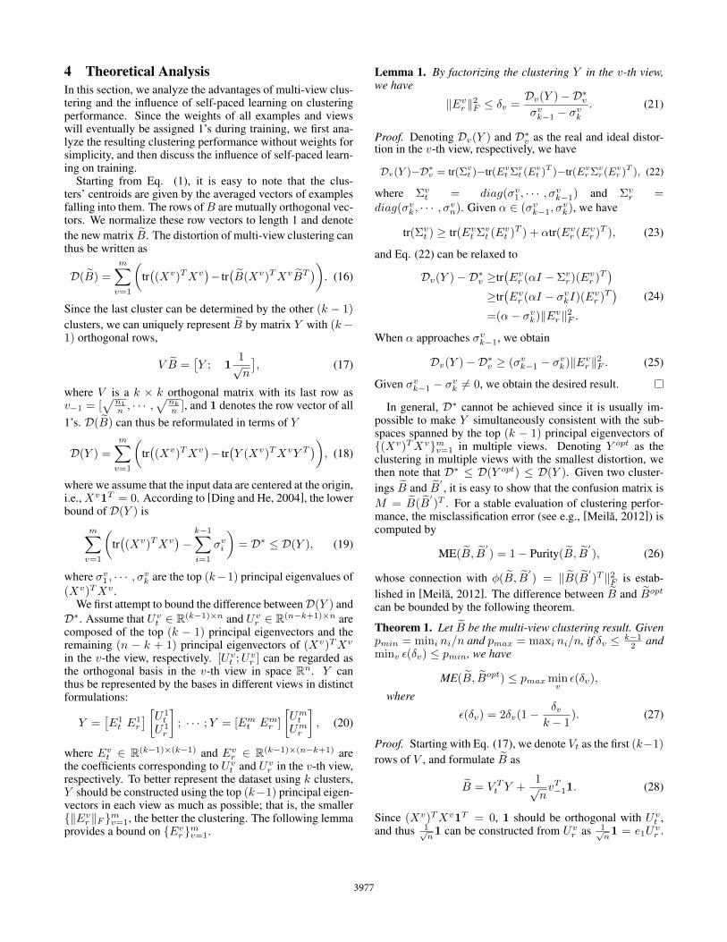
Figure 2: Illustrations on the complexities across examples ((a) in view-1, (b) in view-2 and (c) in view-3) and views (d).

Table 3: NMI comparisons of different multi-view clustering algorithms on the WebKB dataset.

Datasets Con-MC CCA PairwiseSC CentroidSC ConvexSub MSPLCornell 0.094± 0.003 0.090± 0.003 0.112± 0.002 0.104± 0.002 0.233± 0.001 0.215± 0.002Texas 0.143± 0.005 0.120± 0.002 0.179± 0.002 0.169± 0.002 0.245± 0.004 0.255± 0.003Washington 0.159± 0.007 0.223± 0.003 0.212± 0.002 0.185± 0.002 0.251± 0.004 0.281± 0.005Wisconsin 0.090± 0.002 0.092± 0.002 0.098± 0.001 0.108± 0.002 0.303± 0.003 0.337± 0.002

Table 2: Performance on the Animal with attribute dataset.Methods NMI ACC PurityCH 0.077± 0.003 0.067± 0.002 0.087± 0.002LSS 0.081± 0.005 0.071± 0.002 0.088± 0.002PHOG 0.069± 0.003 0.069± 0.004 0.082± 0.004ColorSIFT 0.086± 0.004 0.072± 0.003 0.088± 0.003SIFT 0.094± 0.005 0.073± 0.003 0.091± 0.004SURF 0.088± 0.003 0.076± 0.003 0.097± 0.004Con-MC 0.107± 0.003 0.080± 0.001 0.100± 0.001RMKMC 0.117± 0.005 0.094± 0.005 0.114± 0.005MSPL 0.132± 0.002 0.115± 0.003 0.126± 0.002

added to Gaussian noise, while the remaining entries areadded to uniform noise. Denote the MSPL algorithm withclassical hard weighting (i.e., Eq. (4)) as MSPL-hard, andthat with proposed smoothed weighting (i.e., Eq. (6)) asMSPL-smooth. We compare these two weighting schemeson the toy noisy dataset. As an in-depth analysis on the be-havior of the regularizers, we plot the curves of NMI, ACCand Purity with respect to iterations using hard and smoothedweighting schemes in Figure 3. For easy comparison, we alsoreport the performance of multi-view clustering without self-paced learning (denoted MSPL-naive), as shown in Eq. (2). Itcan be seen that both regularizers can eventually discover bet-ter clusterings than that of MSPL-naive. Compared with theMSPL-hard that is seriously perturbed in the first few itera-tions, the smoothed weighting delivers more accurate results,thus demonstrating the stability of smoothed weighting. Forthe advantages of smoothed weighting, we mainly focus onthe evaluations on MSPL-smooth in what follows.

5.2 Multi-view Clustering ComparisonsWe first evaluate the advantages of multi-view clusteringover single-view clustering on the Handwritten Numerals

and Animal with attribute datasets. The Handwritten Nu-merals dataset is composed of 2000 examples from 0 to 9ten-digit classes. Six kinds of features are used to repre-sent each example; that is, Fourier coefficients of the char-acter shapes (FOU), profile correlations (FAC), Karhunen-Love coefficients (KAR), pixel averages in 2 × 3 windows(PIX), Zernike moment (ZER), and morphological features(MOR). The Animal with attribute dataset contains 30475 ex-amples from 50 classes and described by six features: ColorHistogram (CH), Local Self-Similarity (LSS), PyramidHOG(PHOG), SIFT, colorSIFT, and SURF.

The clustering results on the Handwritten Numerals andAnimal with attribute datasets are presented in Tables 1 and2, respectively. In Con-MC, the features are concatenatedon all views and then standard k-means clustering is applied.It can be seen that employing multiple views leads to im-proved clustering performance than using each view indepen-dently, demonstrating the benefits of integrating the informa-tion from different views. Moreover, all the multi-view clus-tering algorithms are better than the single-view clustering,and MSPL’s clustering is even better than those of multi-viewalgorithms Con-MC and RMKMC. This is because that Con-MC neglects the connections between different views whileconcatenating them for clustering, and RMKMC is likely tofall into a bad local minima due to its non-convex objectivefunction.

We next compare different multi-view clustering algo-rithms on the WekKB dataset, which contains webpages col-lected from four universities: Cornell, Texas, Washington andWisconsin. The webpages are distributed over five classes:student, project, course, staff, and faculty. ‘Content’ and‘link’ are two views that describe each webpage.

The clustering performance in terms of NMI is reported inTable 3. Specifically, on the Washington dataset, the NMIof MSPL improves about 26% over that of CCA and 51%

3979

over that of CentroidSC. The performance of MSPL is similarto that of ConvexSub, which is an elaborately designed con-vex algorithm that discovers the subspace shared by multipleviews. It is instructive to note that MSPL decreases the riskof falling into bad local minima by carefully conducting clus-tering starting from ‘easy’ to ‘complex’ examples and views.On the other hand, ConvexSub separates the multi-view clus-tering task into two steps: learning the subspace shared bydifferent views and launching k-means in this subspace. To-gether, this two-step approach carries a risk of bad local min-ima when clustering.

6 ConclusionIn this paper, we propose multi-view self-paced learning forclustering, which could overcome the drawback of bad localminima during optimization inherent in most existing non-convex multi-view clustering algorithms. Inspired by self-paced learning, the multi-view clustering model is trainedstarting from ‘easy’ to ‘complex’ examples and views. Asmoothed weighting scheme provides a probabilistic inter-pretation of the weights of examples and views. The ad-vantages of using multiple views for clustering and the in-fluence of self-paced learning on clustering performance areanalyzed theoretically. Experimental results on toy and real-world datasets demonstrate the advantages of the smoothedweighting scheme and the effectiveness of progressing from‘easy’ to ‘complex’ examples and views when clustering.

AcknowledgmentsThe work was supported in part by Australian ResearchCouncil Projects FT-130101457, DP-140102164 and LP-140100569, NSFC 61375026, 2015BAF15B00 and JCYJ20120614152136201.

References[Cai et al., 2013] Xiao Cai, Feiping Nie, and Heng Huang. Multi-

view k-means clustering on big data. In IJCAI, pages 2598–2604.AAAI Press, 2013.

[Chaudhuri et al., 2009] Kamalika Chaudhuri, Sham M Kakade,Karen Livescu, and Karthik Sridharan. Multi-view clustering viacanonical correlation analysis. In ICML, pages 129–136. ACM,2009.

[Dalal and Triggs, 2005] Navneet Dalal and Bill Triggs. His-tograms of oriented gradients for human detection. In CVPR,volume 1, pages 886–893, 2005.

[Dalal et al., 2006] Navneet Dalal, Bill Triggs, and CordeliaSchmid. Human detection using oriented histograms of flow andappearance. In ECCV, pages 428–441. Springer, 2006.

[de Sa, 2005] Virginia R de Sa. Spectral clustering with two views.In ICML workshop on learning with multiple views, pages 20–27,2005.

[Ding and He, 2004] Chris Ding and Xiaofeng He. K-means clus-tering via principal component analysis. In ICML, page 29. ACM,2004.

[Ding et al., 2005] Chris HQ Ding, Xiaofeng He, and Horst D Si-mon. On the equivalence of nonnegative matrix factorization andspectral clustering. In SDM, volume 5, pages 606–610. SIAM,2005.

[Guo, 2013] Yuhong Guo. Convex subspace representation learn-ing from multi-view data. In AAAI, volume 1, page 2, 2013.

[Kumar et al., 2010] M Pawan Kumar, Benjamin Packer, andDaphne Koller. Self-paced learning for latent variable models.In NIPS, pages 1189–1197, 2010.

[Kumar et al., 2011a] Abhishek Kumar, Piyush Rai, and HalDaume. Co-regularized multi-view spectral clustering. In NIPS,pages 1413–1421, 2011.

[Kumar et al., 2011b] M Pawan Kumar, Haithem Turki, Dan Pre-ston, and Daphne Koller. Learning specific-class segmentationfrom diverse data. In ICCV, pages 1800–1807. IEEE, 2011.

[Laptev et al., 2008] Ivan Laptev, Marcin Marszalek, CordeliaSchmid, and Benjamin Rozenfeld. Learning realistic human ac-tions from movies. In CVPR, pages 1–8, 2008.

[Liu et al., 2013] Jialu Liu, Chi Wang, Jing Gao, and Jiawei Han.Multi-view clustering via joint nonnegative matrix factorization.In SDM, volume 13, pages 252–260. SIAM, 2013.

[Meila, 2006] Marina Meila. The uniqueness of a good optimumfor k-means. In ICML, pages 625–632. ACM, 2006.

[Meila, 2012] Marina Meila. Local equivalences of distances be-tween clusteringsa geometric perspective. Machine Learning,86(3):369–389, 2012.

[Nguyen et al., 2013] Cam-Tu Nguyen, De-Chuan Zhan, and Zhi-Hua Zhou. Multi-modal image annotation with multi-instancemulti-label lda. In IJCAI, pages 1558–1564. AAAI Press, 2013.

[Oliva and Torralba, 2001] Aude Oliva and Antonio Torralba. Mod-eling the shape of the scene: A holistic representation of thespatial envelope. International journal of computer vision,42(3):145–175, 2001.

[Tang et al., 2012] Kevin Tang, Vignesh Ramanathan, Li Fei-Fei,and Daphne Koller. Shifting weights: Adapting object detectorsfrom image to video. In NIPS, pages 638–646, 2012.

[Wu and Rehg, 2008] Jianixn Wu and James M Rehg. Where ami: Place instance and category recognition using spatial pact. InCVPR, pages 1–8, 2008.

[Xie and Xing, 2013] Pengtao Xie and Eric P Xing. Multi-modaldistance metric learning. In IJCAI, pages 1806–1812. AAAIPress, 2013.

[Xu et al., 2013] Chang Xu, Dacheng Tao, and Chao Xu. A surveyon multi-view learning. arXiv preprint arXiv:1304.5634, 2013.

[Xu et al., 2014] Chang Xu, Dacheng Tao, and Chao Xu. Large-margin multi-view information bottleneck. IEEE Trans. PatternAnalysis and Machine Intelligence, 36(8):1559–1572, 2014.

[Xu et al., 2015] Chang Xu, Dacheng Tao, and Chao Xu. Multi-view intact space learning. IEEE Trans. Pattern Analysis andMachine Intelligence, 2015.

[Zhao et al., 2015] Qian Zhao, Deyu Meng, Lu Jiang, Qi Xie,Zongben Xu, and Alexander G Hauptmann. Self-paced learningfor matrix factorization. In AAAI, 2015.

[Zhou and Burges, 2007] Dengyong Zhou and Christopher JCBurges. Spectral clustering and transductive learning with multi-ple views. In ICML, pages 1159–1166. ACM, 2007.

3980