POLITECNICO DI MILANOCorso di Laurea Magistrale in Ingegneria Informatica

Dipartimento di Elettronica, Informazione e Bioingegneria

Multi-View Learning Through Different

Levels of Abstraction

Extracted by Deep Neural Networks

Relatore: Prof. Pier Luca Lanzi

Correlatore: Prof. Philip S. Yu

Tesi di Laurea di:

Vittorio Selo, matricola 835932

Anno Accademico 2015-2016

Ringraziamenti

Come prima cosa voglio ringraziare il mio advisor, il professor Pier Luca

Lanzi, per essere sempre stato disponibile, per avermi aiutato a completare

questo lavoro e per le piacevoli conversazioni. Ringrazio anche Sihong, Kevin

e Vahid, per avermi aiutato nello sviluppo e per i piacevoli e stimolanti di-

aloghi. Inoltre ringrazio anche i miei professori americani Piotr a Yu per

l’aiuto dato. In aggiunta vorrei anche ringraziare tutti i miei amici che mi

hanno supportato durante questo lungo viaggio (Ale, Ugi, Mavi, Ga, Pippo,

Zanna, Diego, Luca etc.), siete troppi quindi non arrabbiatevi se non ho

scritto il vostro nome. Ringrazio anche tutti i nuovi compagni che ho conosci-

uto grazie al percorso universitario da me intrapreso e con cui ho condiviso

delle esperienze indimenticabili (Benny, Andrea, Da, Andre’,Robi, Fede e

Ettore) Infine, voglio ringraziare dal profondo la mia famiglia (Mamma,

Papa, Zio, Luisa, Aga e anche Stasia), perche senza di loro tutto cio non

sarebbe stato possibile.

VS

i

ii

Sommario

L’obiettivo della presente tesi si concentra sul combinare due nuovi approcci

che oggigiorno stanno diventando sempre piu importanti, cioe deep learning

e multi-view learning.

Il termine deep-learning fu coniato nell’ultimo decennio quando Geoffrey

Hinton e Ruslan Salakhutdinov, nel loro lavoro [22], hanno mostrato che in-

crementando il numero di layer delle feed-forward neural network, un tipo

di Artificial Neural Network (ANN), le performance incrementano, abbat-

tendo quello che fino ad allora era stato il piu grosso limite di quel modello

matematico. In questo lavoro hanno adottato un pre-training stage, dove i

parametri di ogni livello erano tarati utilizzando un unsupervised learning

come se fossero delle Restricted Boltzman Machine (RBM), seguito da un

fine tuning stage. Da allora, Deep Learning (DL) e diventato sempre piu

importante fino al punto di diventare una parte chiave in differenti sistemi

per varie discipline. I campi principali sono Automatic Speech Recogni-

tion (ASR) e Visual Recognition (VR). Differenti tipologie di reti sono

state utilizzate, e alcune di loro hanno raggiunto lo stato dell’arte, in fatti

sono in grado di ottenere i migliori risultati. Per esempio, le Convolutional

Neural Networks (CNN) sono le architetture piu performanti per i compiti

che riguardano il riconoscimento di immagini. Tutto cio e stato possibile per

via dei seguenti motivi: dataset piu grandi, algoritmi piu efficenti e migliori

e l’avanzamento tecnologico che ha permesso veloci computazioni tramite

l’utilizzo della Graphics Processing Units (GPU).

D’altro canto, oggigiorno, abbiamo a disposizioni diverse fonti dalle quali

prendere dati e informazioni per svolgere i compiti che a noi interessano. At-

traverso l’utilizzo di internet, possiamo avere accesso a diverse descrizioni.

Per esempio, su un sito possiamo trovare sia le immagini sia il testo che

rappresentano lo stesso evento, o vari giornali possono parlare dello stesso

avvenimento e di conseguenza avremo punti di vista differenti. L’obiettivo

del Multi-View Learning (MVL) e quello di incrementare le performance e

migliorare i risultati sfruttando le informazioni concordi e complementari tra

iii

le diverse sorgenti. Uno dei primi algoritmi per MVL fu introdotto da Blum e

Mitchell [5] ed e chiamato co-training. In questo lavoro, loro provano a mas-

simizzare l’“agreement” di due differenti viste. Anche in questo caso, i fattori

abilitanti sono stati la possibilita di accedere a dataset piu grandi e la tec-

nologia a cui abbiamo accesso oggigiorno. Comunque, anche se abbiamo

a disposizione dataset piu grandi, ogni tanto e troppo costoso collezionare

dati da sorgenti diverse o semplicemente non abbiamo a disposizione cosı

tante “viste”. E possibile che non abbiamo abbastanza informazioni o che

abbiamo accesso solamente a una sorgente. Per evitare questo problema,

diverse tecniche sono state adoperate con l’obiettivo di estrarre “multiple

views” da una sola vista.

Questa ricerca combina DL con le tecniche di MVL basandosi sulla

seguente intuizione. Solitamente, in una Deep Neural Network (DNN) noi

usiamo solamente le “features” dell’ultimo livello per fare la predizione igno-

rando tutte le features che abbiamo estratto dai precedenti livelli nascosti.

L’idea di sottofondo di questa tesi e di trattare ogni livello della rete come

una vista diversa dell’oggetto originale e combinarle con l’obiettivo di incre-

mentare le performance delle classiche DNN.

Per quanto riguarda la mia conoscenza, questo e il primo tentativo nella

letteratura e differenti approcci sono esplorati in questo lavoro.

iv

Contents

Ringraziamenti i

Sommario iii

List of Figures vii

Acronyms ix

1 Introduction 1

1.1 Thesis Objective . . . . . . . . . . . . . . . . . . . . . . . . . 3

1.2 Thesis Structure . . . . . . . . . . . . . . . . . . . . . . . . . 4

2 Background Knowledge 5

2.1 Deep Learning . . . . . . . . . . . . . . . . . . . . . . . . . . 5

2.1.1 Artificial Neural Network . . . . . . . . . . . . . . . . 5

2.1.2 Artificial Neural Networks - Concepts . . . . . . . . . 6

2.1.3 Deep Learning - Concepts . . . . . . . . . . . . . . . . 13

2.2 Multi-View Learning . . . . . . . . . . . . . . . . . . . . . . . 15

2.2.1 Multi-View Learning - Concepts . . . . . . . . . . . . 15

2.2.2 Multi-View Learning - View Generation . . . . . . . . 16

2.2.3 Multi-View Learning - View Evaluation . . . . . . . . 17

2.2.4 Multi-View Learning - View Combination . . . . . . . 17

2.3 Tools and GPU . . . . . . . . . . . . . . . . . . . . . . . . . . 19

3 State of The Art 21

3.1 Convolutional Neural Network . . . . . . . . . . . . . . . . . 21

3.1.1 Convolutional Neural Network - Convolutional Layer . 22

3.1.2 Convolutional Neural Network - Pooling Layer . . . . 23

3.1.3 Convolutional Neural Network - ReLU and Activation

Functions . . . . . . . . . . . . . . . . . . . . . . . . . 24

3.1.4 Neural Network - Dropout . . . . . . . . . . . . . . . . 26

v

3.1.5 Convolutional Neural Network - Case Studies . . . . . 27

3.2 Multi-View Learning . . . . . . . . . . . . . . . . . . . . . . . 27

3.2.1 Multi-View Feature Learning . . . . . . . . . . . . . . 28

4 Objective and Model Description 31

4.1 Objective . . . . . . . . . . . . . . . . . . . . . . . . . . . . . 31

4.2 Model . . . . . . . . . . . . . . . . . . . . . . . . . . . . . . . 33

4.2.1 Framework Description - Stage One . . . . . . . . . . 34

4.2.2 Framework Description - Stage Two . . . . . . . . . . 35

5 Evaluation 39

5.1 Experiment A . . . . . . . . . . . . . . . . . . . . . . . . . . . 39

5.2 Experiment B . . . . . . . . . . . . . . . . . . . . . . . . . . . 43

5.3 Experiment C . . . . . . . . . . . . . . . . . . . . . . . . . . . 45

5.4 Experiment D . . . . . . . . . . . . . . . . . . . . . . . . . . . 50

5.5 Experiment E . . . . . . . . . . . . . . . . . . . . . . . . . . . 54

6 Conclusion 57

Bibliography 59

vi

List of Figures

2.1 Schema of a neuron. . . . . . . . . . . . . . . . . . . . . . . . 8

2.2 Artificial neural network. . . . . . . . . . . . . . . . . . . . . 8

2.3 Nesterov momentum. . . . . . . . . . . . . . . . . . . . . . . . 12

2.4 Sustkever momentum. . . . . . . . . . . . . . . . . . . . . . . 12

3.1 Convolutional schema. . . . . . . . . . . . . . . . . . . . . . . 23

3.2 Max pooling schema. . . . . . . . . . . . . . . . . . . . . . . . 24

4.1 Ann schema. . . . . . . . . . . . . . . . . . . . . . . . . . . . 32

4.2 Single view approach. . . . . . . . . . . . . . . . . . . . . . . 35

4.3 Multi-view learning schema. . . . . . . . . . . . . . . . . . . . 37

5.1 Multi-view feature learning - experiment a - weights. . . . . . 42

5.2 Multi-view feature learning - experiment b - weights. . . . . . 46

5.3 Multi-view feature learning - experiment c - weights. . . . . . 49

5.4 Multi-view feature learning - experiment d - weights. . . . . . 53

vii

viii

Acronyms

ANN Artificial Neural Network

RBM Restricted Boltzman Machine

DL Deep Learning

ASR Automatic Speech Recognition

VR Visual Recognition

CNN Convolutional Neural Networks

GPU Graphics Processing Units

MVL Multi-View Learning

DNN Deep Neural Network

CAP Credit Assignment Path

MKL Multiple Kernel Learning

ILSVRC ImageNet Large Scale Visual Recognition Competition

ix

x

Chapter 1

Introduction

Nowadays, Data Mining is getting more and more valuable for many differ-

ent industry branches. In order to understand the motivation, first we need

to explain what Data Mining is.

Data mining is an interdisciplinary field under computer science that uses

different techniques (e.g. machine learning, artificial intelligence, statistics)

in order to discover patterns in datasets [7]. These patterns should represent

useful and not naive information.

The first terms that were used to refer to this practise were: “data fish-

ing” or “data dredging” and they appeared around 1960. During the 1980s

a new word appeared, namely “database mining”. However, since it was a

trademark of a company in San Diego, the researchers, around the 1990s,

decided to change the terminology in “data mining” and this name persisted

to this day [31]. Nowadays there are two equivalent terms used to refer to

this sub-field: knowledge Discovery or data mining.

Data mining is a still growing field, but all these started in 1995 when the

first international conference about data mining took place - it was named

Knowledge Discovery and Data Mining(KDD) - and it is still one of the

most famous conference in the world.

The final goal of data mining is to find hidden patterns in large data sets

through automatic methods that we can access thanks to the development

of computer science technologies.

The process is the following one:

Selection: First of all, a problem we want to face need to be selected,

then we gather data and get information in order to have a better

understanding and see possibilities to exploit the domain knowledge.

Pre-processing: This step is essential for good results. Often, the data we

1

have can be noisy or have some null values, so we have to decide how

to treat them and how to solve the issues.

Data Mining: This is the core of the whole process where our model is

built. Here, the attention is paid on different techniques based on

what our purpose is. For example, we can perform anomaly detection

(identification of the outliers),clustering or a more traditional classifi-

cation.

Evaluation, validation and interpretation: Here, our hypothesis is val-

idated with unseen data or simply by discussing the results. It needs

to be verified how good our model is and an interpretation on what

we have discovered ought to be given. Usually, the results are good

because our model or the data we have used were excellent. However,

given interpretation and explanation are the most valuable part for

the companies.

Of course, corporations are interested in such kind of data analysis. In

the last two decades, the technology has improved so much that the com-

panies were forced to adapt and change their business model exploiting

computer science in order to gain advantage over competitors. Today, it is

not possible to think about a successful company without an information

system.

In order to stay competitive and survive, they start to gather data about

their clients and customize their services. The final goal is to “mine” valu-

able knowledge from all these data to give or keep a strategic advantage.

Currently, these techniques are most used in business intelligence, customer

analytic and decision support system. These domains are considered the

most beneficial from a business point of view.

In addition, with the spread of Internet on a global scale, companies

have to worry about their image on social media as well as their relationship

with the clients. In effect, if they are not able to manage such situations, it

is more harmful than anything else. But, there are not only disadvantages.

The companies can use social media data to have a general idea on how well

they are doing and how to correct their decisions in order to improve their

strategy or offer better services. For example, in [51] the authors showed

how using Twitter data, may help to increase the performance of a recom-

mendation system exploiting homophily.

However, another field that benefits from data mining techniques is bioin-

formatics. Bioinformatics exploits computer science software in order to

have a better understanding of biological data. Therefore, it may be said

2

that data mining plays a key role here. Thanks to the technologies develop-

ment, today we have access to abundant data regarding proteins, molecules

and genes. We can exploit data mining technique to make protein structure

prediction and many other tasks as shown in [38]. As an example, in [15]

the authors have used diffusion maps [11], a dimensionality reduction tech-

nique, to have a low dimensionality description of their data and perform

the analyses in a more straightforward way.

These are only a few examples of using data science, but it has a lot

more applications. We can find it in educational system with natural lan-

guage processing, fraud detection, automatic stars classification and many

other fields. In addition, more and more fields are using data mining to

achieve better results and new knowledge. For example, neuroscientists are

using it to understand relations between different regions of our brain.

It is a constantly evolving and, in the recent years,many new branches

have been born such as big data analysis or graph mining.

In conclusion, data science is a growing field where the only and real

limit we have is our creativity and imagination.

1.1 Thesis Objective

The goal is to investigate and discover if previous layers in ANNs can con-

tain useful and unexploited information to increase the performance of our

task.

Practical evidence have showed that the more layers we have the more

accurate will be the prediction and generally speaking it is true, previous

layers are less precise if they are taken by their own. However, for the best

of my knowledge, no one have tried to combine different layers together. We

can see each level as a latent-subspace into which we are projecting our input

data. Since the training phase is not constrained, in some layers there may

be group of features that are more discriminative and precise to describe a

certain type of object, hence a label. Maybe in a certain latent-subspace is

more easily to distinguish between two classes, moreover it is possible that

we are losing this information.

To study this behaviour we will propose a framework that is a combina-

tion of two well know methods traditional neural networks and MVL models.

Summing up, the objective of this work is to understand if previous lay-

ers of ANNs can have knowledge that can be exploited in order to achieve

better results.

3

1.2 Thesis Structure

The structure of this work will be the following one. In chapter 2 we will

explain general concept that are needed to understand properly the thesis,

we will talk about ANN and DL, then we will explain MVL concepts and

in the end the tools used. In chapter 3 we will talk about the state of the

art and we will cover all the details of the methods we are going to use. In

chapter 4 we will introduce the proposed framework for the research and in

chapter 5 we will report the results of the conducted experiments. In the

end, in chapter 6 we will summarize and talk about the conclusions and

implications of this work.

4

Chapter 2

Background Knowledge

In this chapter the discussion is going to point to the basic knowledge needed

to understand the present work. Also, a common vocabulary will be intro-

duced in order to avoid misunderstandings.

In Section 2.1 we will introduce the basic concepts of deep learning,

the models that will be used in this work as well as historical background.

Furthermore, in Section 2.2 we will talk about basic notions of multi-view

learning. Finally, in the last part, Section 2.3, we will talk about the tools

we have used and some present elementary knowledge about GPU and GPU

programming.

2.1 Deep Learning

Before explaining what deep learning is, a term artificial neural network

(ANN)needs to be introduced, as the models we are going to exploit are

based on it.

2.1.1 Artificial Neural Network

Until today, the most amazing “computer” one could think of about is our

brain.It can effortlessly recognized subjects in a pictures or images, analyz-

ing the color and attributes it is easy to identify what we are looking at.

People have no problems to understand speech or text messages. All these

operations are natural and simple for us, but doing them automatically and

by the use of software is not so trivial. As a natural consequence, researchers

have been inspired by our brains. Based on what is known and what is still

being discovered about this mysterious machine, many models have been

created trying to imitate our cognitive process. In the end, it can be said

that ANNs are a rough approximation of how our thought processes work.

5

Druing the 1943, Warren McCulloch and Walter Pitts in [30] proposed

the first model of an ANN. It was a math model based on thresholds.

A lot of work has been made since 1958, when Frank Rosenblatt ex-

plained in [40] how to create a perceptron, a machine learning algorithm

capable of doing binary classification. In the community there was a lot of

enthusiasm and a lots of effort was put into the research. All this lasted

until 1969, when Marvin Minsky and Seymour Papert in [32] showed the

limits of a single-layer perceptron, that was not capable of approximate all

type of functions and highlighted the limits caused by the computational

power they had access to. Even if, they said nothing about multiple-layers

and networks, this was an earthquake that blocked the research for several

years.

This black era terminates in 2006 for different factors. First, in 1989

universal approximation theorem was proved by George Cybenko [13], who

stated:

“The standard multilayer feed-forward networks with a single hidden

layer that contains finite number of hidden neurons, and with arbitrary ac-

tivation function are universal approximators in C(Rm). ” [12].

Once for all, thanks to the proof of this theorem, the networks of per-

ceptrons have no more limits.

Then, on account of the new computational power and mathematical

algorithms, Geoffrey Hinton and Ruslan Salakhutdinov in [22] showed that

it was possible to rise the performance of a feed-forward neural network in-

creasing the number of layers and adopting a suitable algorithm. In order to

achieve their result they have pretrained all the layers with RBM and then

they have fine tuned all the networks with the traditional back propagation

algorithm.

This was the start of a new era for neural networks that have become a

very useful tool exploited in different fields, especially machine learning and

data mining.

After this brief historical introduction on ANN,their functionalities can

be explained.

2.1.2 Artificial Neural Networks - Concepts

ANNs are a graphical model. As in any graph, even there are nodes and

edges. Let us start with the nodes.

Each node is called a neuron, in analogy with our brains. It is simply

a mathematical function f : X → Y that tries to imitate the behaviour of

real neurons. Here, X is the domain input of dimension m, Y is the domain

6

output and usually it is mono dimensional and indicates the activation of

the neuron itself.

So, it can be said that each neuron will receive a vector as input. The

usual way to combine each input is to perform a weighted sum. Conse-

quently, a weighted vector is the essence of our node. In fact, as in our

brain, each input is weighed because some input is more relevant for a task

than others (that means a bigger weights), or they can be useless so they are

not taken into consideration (zero or small weights). Thinking abstractly,

the weighted vector represents the functionality. The weighted sum of the

inputs is forwarded to the activation function. There are different activation

function, for example:

Step function: It is the following function{1 if u ≥ θ0 if u < θ

(2.1)

Usually, θ is a fixed threshold and since the inputs are usually normal-

ized, we set θ = 0.5 if the inputs are in the range 0 to 1, or 0 if the

inputs are in the range -1 to 1. This function was used in the percep-

tron, and can be only used in linear patter, so it is not able to represent

functions like the XOR. It is very useful if binary classification needs

to be performed.

Linear combination functions: In this category fall all the linear models.

Usually, the output is simply the weighted sum plus a bias term.

Sigmoid function: It was one of the first functions that was used, however

for different problems it is not used any more. It is a non linear function

and it is simple to calculate the derivative, that is very important to

learn the weights. The sigmoid function is the following one:

S(t) =1

1 + e−t(2.2)

Hyperbolic tangent: It is another “famous” activation function. It is

always preferable to use instead of the sigmoid function, as it solves a

problem. In fact it has the nice property to be symmetric around the

zero. It has the following math formula:

tanh(t) =sinh(t)

cosh(t)=et − e−t

et + e−t=e2t − 1

e2t + 1=

1 + e−2t

1− e2t(2.3)

7

Activation function

∑w2x2

......

wnxn

w1x1

w0x0

inputs weights

Figure 2.1: Schema of a neuron.

Input #1

Input #2

Input #3

Input #4

Output

Hidden

layer

Input

layer

Output

layer

Figure 2.2: Artificial neural network.

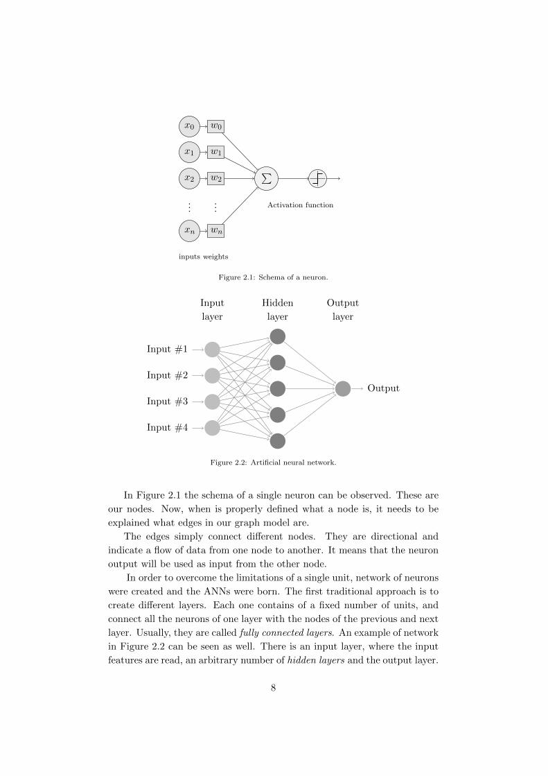
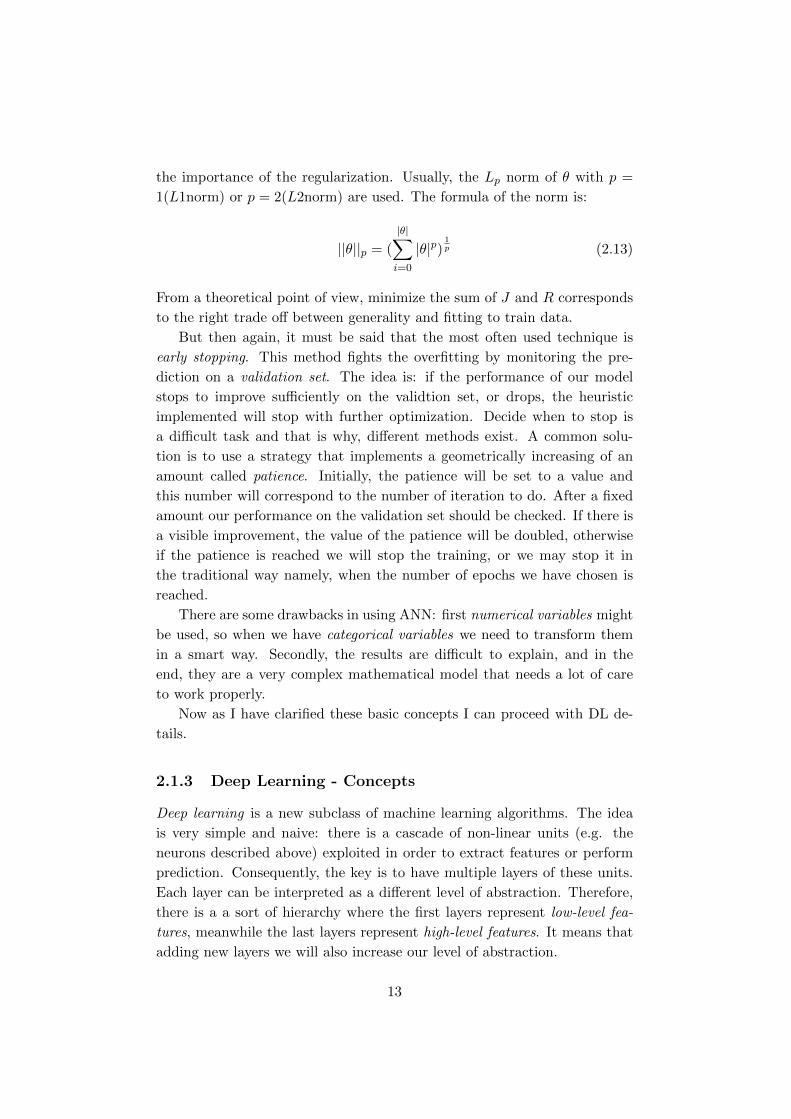
In Figure 2.1 the schema of a single neuron can be observed. These are

our nodes. Now, when is properly defined what a node is, it needs to be

explained what edges in our graph model are.

The edges simply connect different nodes. They are directional and

indicate a flow of data from one node to another. It means that the neuron

output will be used as input from the other node.

In order to overcome the limitations of a single unit, network of neurons

were created and the ANNs were born. The first traditional approach is to

create different layers. Each one contains of a fixed number of units, and

connect all the neurons of one layer with the nodes of the previous and next

layer. Usually, they are called fully connected layers. An example of network

in Figure 2.2 can be seen as well. There is an input layer, where the input

features are read, an arbitrary number of hidden layers and the output layer.

8

An ANN may possibly be used in two ways: to make prediction based on the

labels or to extract features. However, in both cases a learning algorithm is

needed. This procedure is very meaningful and it is the core of an ANN.

Here, the weights are being learnt, or in other words, the parameters with

which we are going to approximate the function that links the input data

with the label of our interest.

So, the learning objective is to approximate a function, but how is it

going to be done? First of all, we need a cost function we want to optimize.

Generally speaking, it needs to have some desirable proprieties such as:

convexity and the optimal solution should be a global minimum. In this

way, the problem may be faced as a mathematical optimization and we can

learn the function depending on the weights of the network. After that, it

is set up. The learning paradigms may be divided into two categories:

Supervised Learning: In this situation our data are composed by a couple

(x, y). Where X are the input features and Y is the class of our

interest. Our aim is to learn the function f : X → Y . In this case, the

most common cost function is the mean-squared error.

Unsupervised Learning: In this context, there is only our data x and

the cost function to be minimized which relies on x and the output

of the network. It also depends on the a priori assumption that have

been made.There are a lot of cost functions and they may be very

complicated. A famous typology of network for unsupervised learning

is autoencoders.

The most often used learning algorithm is backward propagation of errors

or abbreviated backpropagation. The general idea is to calculate the gradient

of our function in order to reach a minimum based on the derivative that

will modify the weights of our network. In other words, we will update our

parameters based on the error made on a set of samples. We will feed the

training data to the network multiple times, each time is called epoch.

For instance, if there is the following function:

J(θ0, θ1) that can be generalized to: J(θ0, ..., θn) (2.4)

What we want is:

minθ0,θ1

J(θ0, θ1) that can be generalized to: minθ0,...,θn

J(θ0, ..., θn) (2.5)

Where: θ0 and θ1 are the parameters of our function, or in other words

the weights. Additionally, in order to to be feasible, we need a derivable

9

activation function for our neurons. At the beginning, the sigmoid function

was a common and good choice because it has the following nice derivative.

dS(t)

dt= S(t)(1− S(t)) (2.6)

But, nowadays it is not used any more because it has some relevant problems,

so other activation functions were adopted as tanh. We are going to update

our parameters exploiting partial derivative and chain rule through gradient

descent. The update will be performed by using the following equation:

θi := θi − αδ

δθiJ(θ0, ..., θn) (2.7)

Where α is an important hyper-parameter, the learning rate. It influences

the speed and quality of the learning. The bigger it is, the faster the weights

will change. The smaller it is, the slower the change will be, but generally

speaking it will also be more accurate.

However, as computing the analytical derivative is very expensive, the

numerical derivative is used. Each unit will store the local gradient and will

update the weights when it receives the local gradient from the next units

during the back-propagation stage. It will be faster and computing the real

derivative is not needed. But, the drawback is that all the local gradient

need to be saved in memory and they can be removed only after the back-

propagation.

Now, the methods to perform the updates may be formally introduced:

Gradient descent (batch): With this method we are using all the train-

ing examples at once in order to minimize the function problem. It is

the most accurate optimization, but it is also expensive if there are a

lot of data. It calculates the derivative and sums the gradients of all

the samples and only after this it will update the weights.

Stochastic Gradient Descent: With this method we are not looking to

all the training examples, but we just use one sample at a time. So,

the question is how well we are doing with respect one example. Con-

sidering the mean squared error E = 12(hθ(x)− y)2, the cost function

will be modified as follows:

cost(θ, (xi, yi)) =1

2(hθ(x

i)− yi))2 (2.8)

Consequently, the updates will be modified in this manner:

θj := θj − α(hθ(xi)− yi)xij (2.9)

10

It simply means that we update our parameters considering the cost

of the i− th sample. The fundamental issue is to shuffle our samples

randomly as we do not want all the objects with the same label to-

gether. Moreover, if α is set with a constant, as in the majority of

the algorithms, there is no guarantee that the global minimum will

be reached, however it can be good enough to get near it. If we

want to reach it, α can be slowly decrease over time. For instance,

α = k1Iteration number +k2

. However, people are not willing to use this

implementation because there are more parameters to choose from in

order to have a good learning rate.

Mini-Batch Gradient Descent: It is the middle way. In the batch case

all the training examples are used. In the stochastic case just one is

analysed. In mini-batch one decides about a size of b and analyses b

examples in order to calculate our cost function. So, instead of using

one examples we are going to use b examples. Therefore, the updates

formula changes in the following way:

θj = θj − α1

b

i+b−1∑k=i

(hθ(xk)− yk)xkj (2.10)

Where i will start from 0 and at each iteration will increase of b. The

only disadvantage of this method is that a new hyper-parameter has

to be chosen. However, the main benefit is the vectorization, in fact if

there is a good one the training may be partially parallelized.

Despite everything mentioned above, there is still a problem. One of

the major concern is to improve the learning speed in the ANN. The best

thing to do is to use mini-batch gradient descent with momentum. The

momentum will remember and keep the previous direction of the gradient

(it is a sort of velocity), but we want to stop it in ultimate time. In order to

achieve this goal we introduce viscosity that will reduce our “velocity” and

allows us to stop in a low point. Consequently, velocity will decrease slowly

each update.

v(t) = αv(t− 1)− εδJδθ

(t) (2.11)

The equation 2.11 is the one that is going to be used and α will be called

momentum. If the momentum is close to one it will be much faster than a

simple gradient descent. Consequently, we do not want a big learning rate

because it means a big divergence. Thus, at the beginning there should be

a small momentum to avoid these bad property. Once the large gradients

disappear, we reach the“normal training” and we can rise the momentum

11

Current Gradient Store Gradient

Combined Gradient

Figure 2.3: Nesterov momentum.

Store Gradient

New Gradient and Combined Gradient

Figure 2.4: Sustkever momentum.

to its ordinary value. The momentum was formulated first time by Yurii

Nesterov in 1983 [34].

In Figure 2.3 the standard method can be seen. First, the gradient

at the current location is calculated, then it is combined with the previous

gradient and in the end a big jump in the combined result is taken.

In 2013 Ilya Sustkever with [43] introduced a new and better method

for the momentum. It is a form of momentum suggested by Nesterov who

was trying to optimize convex function. The idea is to take a big jump in

the direction of the previous gradients, then the gradient where we are is

measured and the correction is performed. We believe it is that is better to

correct a mistake after it has been made.

In Figure 2.4 a graphical representation is shown in order to understand

the differences better.

Now, as all these tools are presented, there is another problem that needs

to be solved. If we perform only the optimization there is a possibility that

we incur in overfitting. A way to avoid or combat overfitting is regularization.

Regularization adds a new term to our cost function that will penalize certain

parameter configurations. More formally, if J is the old cost function, our

new cost function will be:

Jnew = J(θ) + λR(θ) (2.12)

R(θ) is the regularization term and λ is an hyper-parameter that controls

12

the importance of the regularization. Usually, the Lp norm of θ with p =

1(L1norm) or p = 2(L2norm) are used. The formula of the norm is:

||θ||p = (

|θ|∑i=0

|θ|p)1p (2.13)

From a theoretical point of view, minimize the sum of J and R corresponds

to the right trade off between generality and fitting to train data.

But then again, it must be said that the most often used technique is

early stopping. This method fights the overfitting by monitoring the pre-

diction on a validation set. The idea is: if the performance of our model

stops to improve sufficiently on the validtion set, or drops, the heuristic

implemented will stop with further optimization. Decide when to stop is

a difficult task and that is why, different methods exist. A common solu-

tion is to use a strategy that implements a geometrically increasing of an

amount called patience. Initially, the patience will be set to a value and

this number will correspond to the number of iteration to do. After a fixed

amount our performance on the validation set should be checked. If there is

a visible improvement, the value of the patience will be doubled, otherwise

if the patience is reached we will stop the training, or we may stop it in

the traditional way namely, when the number of epochs we have chosen is

reached.

There are some drawbacks in using ANN: first numerical variables might

be used, so when we have categorical variables we need to transform them

in a smart way. Secondly, the results are difficult to explain, and in the

end, they are a very complex mathematical model that needs a lot of care

to work properly.

Now as I have clarified these basic concepts I can proceed with DL de-

tails.

2.1.3 Deep Learning - Concepts

Deep learning is a new subclass of machine learning algorithms. The idea

is very simple and naive: there is a cascade of non-linear units (e.g. the

neurons described above) exploited in order to extract features or perform

prediction. Consequently, the key is to have multiple layers of these units.

Each layer can be interpreted as a different level of abstraction. Therefore,

there is a a sort of hierarchy where the first layers represent low-level fea-

tures, meanwhile the last layers represent high-level features. It means that

adding new layers we will also increase our level of abstraction.

13

Nowadays, for the layers of DL both ANNs or sets of propositional for-

mula [3] may be used. However, the most common choice is to implement

DL with multiple layers of ANN.

Consequently, there will be different stacked layers and it may be pos-

sible to build a path from the input to the output, what is name Credit

Assignment Path (CAP). The CAP is simply a series of non linear trans-

formation. Schmidhuber, in his work [41], considers a value of CAP> 10 to

be a very deep learning.

It may be thought each layer is the representation of a latent space, the

nodes are the latent variables that describes the dimensions and the ex-

tracted features are called latent features. The word latent or hidden may

be used in an equivalent way. So, what is the meaning of latent? With this

word we want to describe something that exists but is not visible. Here, the

idea is that the original data are generated by a latent space in which it is

easier to perform the desired task, therefore the objective is to construct it

through deep learning. However, provide meaning to these features is very

difficult or even impossible. Most of the time they are just numbers, there-

fore it is really problematic to give a reasonable explanation.

In the last years, an increase in the use of DL has been observed. It

was possible for different reasons. First of all, back in 1980, the first deep

learning architecture was invented by Kunihiko Fukushima [16]. However,

they were not able to train multiple layers properly. Moreover, the huge

training time made them not useful in real scenario. We had to wait till the

middle of 2000, when in [22], the authors showed that it was possible to rise

the performance increasing the number of layers. Another enabling factor

was the improvement of hardware, in fact the GPUs are ideal for matrix

calculation and they have speeded up the networks training time by one

order of magnitude. Consequently, now DL is possible to use thanks to the

development of hardware and algorithms.

Since, the method is based on ANN with multiple layers, these networks

are called deep neural networks(DNN). The underline assumption is that

the target object can be represented as a composition of features that are

visible in different layers.

Today, DNNs are the state of the art in various fields as ASR and VR.

Moreover, recurrent neural networks are gaining relevance also in language

modelling.

However, there is no such a thing as a free lunch. Increasing the num-

bers of layers brought new problems. The two main concerns are over-fitting

and the computational time. For the first one, different techniques were de-

veloped and as it was said above they are called regularization method. In

14

addition to the already mentioned methods, one recent successfully regular-

ization approach was introduced by Geoffrey E. Hinton called dropout [23].

Another problem is the computational time. In order to be able to learn

the weights in a deep networks big datasets are needed, otherwise the learn-

ing will not happen. Of course, this increases the time required by the

network to fit the data. Besides, it makes impossible to use a technique

as gradient descent. It has been found that a good compromise is to use

mini-batch with Nesterov momentum.

2.2 Multi-View Learning

Multi-view learning is a new sub field of machine learning that was born

only a few years ago. The purpose of this new class of algorithm is to ex-

ploit different views in order to increase the performance for a task of our

interest.

First of all, it needs to be defined what a view is. A view is a description

of an object from one point of view. For example, on websites the same

object can be described with a photo and text. In this situation the photo

is a view and the text is another view. The underline idea is that different

views can have different information to exploit. Therefore, one can benefit

from combining them in a smart way.

Nowadays, it is gaining more and more relevance because there is tech-

nology to access them and gather a lot of data. Additionally, the key is the

possibility to have different dataset (different views) about the same object

or event. Another example may be newspapers describing the same event,

each text can be seen as a different view.

After it has been defined what a view is, a division of the multi-view

learning algorithm may be introduced. There are three main classes: co-

regularization, Multiple Kernel Learning (MKL) and subspace learning.

Before focussing on each type, we will talk about some principle of MVL.

2.2.1 Multi-View Learning - Concepts

The general idea is to have multiple views about the same input data, so the

learning can exploit abundant information. But, if the learnt algorithm we

are using is not good, there is the real possibility to degrade the performance.

For this reason it is mandatory to use a proper algorithm.

Traditional machine learning methods will just concatenate the features

from the different view in one single view and then apply a single-view

algorithm. This is deeply wrong as each view has its own statistical property.

15

By using a mere concatenation we are going to lose these information so the

results can be even worse and it can occur also in overfitting.

The paradigm is to jointly optimize all the functions from different views

to exploit redundant knowledge for the same input data and increase the

performance.

There are two principles to follow in order to have a successful method:

Consensus Principle: First of all, the agreement between multiple dis-

tinct views needs to be maximized. In [14], the authors have proved

that there is a correlation between the error rate and the agreement

between two views. Thus, maximizing the agreement will decrease the

error rate on each hypothesis.

Complementary Principle: Different views can have complementary in-

formation, this means that they can have different knowledge that

others views do not have. Some of the multi-view algorithms have

been proved to work better when the diversity between the different

learners of the views is bigger [47].

After introduction of these two principles, the attention may be paid on

MVL. While facing a multi-view problem there are three main stages that

need to be considered:

2.2.2 Multi-View Learning - View Generation

During this phase the priority is the acquisition of redundant data from

different points of views. So, it is important not only to gather different

prospective about some attributes, but each single view should be able to

represent the data sufficiently.

Usually, we do not have different views of the same object at our disposal.

However, to solve this problem it is possible to construct different views

starting just from one.

The three classes of view generation can be identify [49]:

• Construction of views from meta-data through random approaches.

An example is Random Subspace Method (RSM) [6] which incorporates

the benefits of bootstrapping and aggregation. In fact, the point is

to select a dimension n and we build up multiple views each one of

dimension n. This method has the peculiarity of taking advantage of

dimensions instead of suffering from the curse of dimensionality.

• Reshape or decompose the original view into multiple views. An ex-

ample of such method is [48], where the authors have created multiple

16

views for a vector representation reshaping the vector in different ma-

trices. The authors also claim that these views can be considered

weakly correlated.

• Automatically feature set partitioning as genetic algorithms or pseudo

mutli-view cotraining (PMC) [8] that derives automatically from a

single view two mutually exclusive subsets of features.

2.2.3 Multi-View Learning - View Evaluation

Another significant aspect is the evaluation of the single views and their

combination in order to ensure that they have a minimum level of quality

for the multi-view learning algorithms.

In fact, it is a common issue that the view sufficiency assumption fails,

it means that our extra data from a view can corrupt the quality and the

information of other views, as a result our performance will be worse.

Moreover, noisy views can influence the performance of the algorithm in

a bad way. As suggested in [9], a solution is to discard the samples that

display a high view disagreement.

A lot of methods were developed to solve this problem, but the most

common answer is to use a validation dataset where one monitor the perfor-

mance of his or her method with different combination of views and remove

the bad ones if necessary.

2.2.4 Multi-View Learning - View Combination

In the last stage an algorithm that combines the knowledge from different

views is needed. As it was already said, the concatenation of all views in a

single view and applying a single view algorithm is not the right way. With

this naive method some problems like overfitting may occur and, what is

more, the pure concatenation is not meaningful from a statistical point of

view.

For these reasons a bunch of methods born in order to take advantage

of the mutual information in multiple-views. The learning methods may be

classified in three categories[49]:

Co-training style: [5] is one of the first works about MVL. It tries to

exploit the mutual information and agreement between different views

in the presence of unlabelled data. It has three assumptions:

Sufficiency: each view should be able to perform a classification on

its own, it means that the single view should be able to beat the

17

naive classifier also known as the majority class.

Compatibility: The different learners of the views should predict the

same label for features that are together with a high probability.

Conditional Independence: Each view is independent from the other

given the target label. However, since it is too difficult to guaran-

tee this property, over the years several weaker alternatives were

proposed .

These styles of algorithms are confidence driven. The idea is to force

similarity between the different learners, we want to maximize the

consistency between them. We will back propagate the disagreement

in order to have more accurate learners. To obtain this goal we will

exchange the information through the validation data.

Co-training was the first attempt, more sophisticated method were de-

veloped as CO-EMT [33], a combination of CO-EM and CO-Testing.

Multiple Kernel Learning (MKL): Originally it was developed to con-

trol the search space capacity of kernels to achieve a good generaliza-

tion. However now, it is largely used in a multi-view context. The

idea is very simple. When applying kernels we get different notion of

similarity and distance, and there is not one that is better than the

other. Thus, the paradigm is to train simultaneously different kernels,

not just pick the best one.

We will apply different kernels to our data and then we combine them

and optimize this new objective function. The kernels may be com-

bined by using linear combination (e.g. direct summation kernel or

weighted summation kernel) or non linear combination (e.g. exponen-

tial or power combination). In this case each kernel is a view on the

data and it is possible to try to combine the different transformation.

Subspace Learning: The objective of this kind of algorithms is to gener-

ate a latent subspace shared by all the views. Here, the assumption

is that multiple views are generated from the same subspace. Prin-

cipal component analysis (PCA) can be viewed as a simple technique

to obtain a subspace from single view data. The multiple view ver-

sion of PCA is canonical correlation analysis (CCA). CCA is a general

tool for multi-view learning. The goal is to maximize the correlation

between different views and obtain their projection in the latent sub-

space. However, CCA applies a linear transformation. Consequently,

Kernel CCA was developed for hard cases. It is a prior combination of

18

the views in order to generate the common latent subspace and then

apply a more traditional algorithm.

These are the main techniques used nowadays for multiple view learning.

2.3 Tools and GPU

In this section, the tools used to implement and perform our experiments

will be described. The language used for the developing part was python

version 2.7. The most used libraries were: numpy and scipy [45] for generic

computations and scikit-learn for the evaluation part [37].

Moreover, in order to speed up the time we have decided to adopt GPU

for the training and testing phase of ANN. In fact, GPUs are perfect for

neural network training as their nature allows them to perform matrices

operation exploiting parallel computation. From a programming point of

view, each layer of an ANN can be viewed as a combination of two tensors:

one for the weights and one for the biases. Also, the input data can be viewed

as a tensor, so they can flow through the network using tensor operations

such summation and dot operation.

In order to use GPU programming we have decided to adopt theano, a

python library [1] [4]. It allows us to define and evaluate tensor operation

and have a transparent use of the GPU.

Theano leans on low level implementation for using GPUs, actually it

generates dynamic C code. Nowadays, there are two main frameworks:

CUDA backend and OpenCL, and both are compatible with theano. As the

machine we have used has a NVIDIA card, we have used CUDA [35].

The code was based on http://deeplearning.net/tutorial/ and the

dropout implementation used is taken from https://github.com/mdenil/

dropout.

Moreover, we have also used the code from https://github.com/mttk/

STL10 to load easily the dataset STL-10.

19

20

Chapter 3

State of The Art

In this chapter the attention will be paid on the state of the art and of

the most popular techniques in the field of ANN and MVL. Moreover, the

details of CNN will be presented as in the experiment phase only images are

going to be used. Then, some methods for MVL and the technique we have

decided to adopt will be introduced.

3.1 Convolutional Neural Network

CNNs are traditional neural networks that make one single and very use-

ful assumption, namely the inputs are images. They have taken inspiration

from how the visual cortex of a cat works [24]. Thus, we can make some sim-

plification exploiting the properties of the images through the architecture

of the network. In fact, we are able to make the the forward function more

efficient and we can decrease significantly the number of needed parameters.

The network will take advantage of the fact that the input is an image

using 3D neurons. There will be three dimensions: width, height and depth.

In fact, any image can be described as a tensor. Usually an RGB can be

viewed as widthxheightx3, where the depth of three represents the 3 colors:

red, green and blue. It can be also widthxheightx1 if we have black and

white pictures, in this case the depth of one represents the intensity where

0 is white and 1 is black. So, in a CNN we are performing transformation

of volumes.

CNNs use the following type of layers: fully connected hidden layers (as

in traditional ANN), convolutional layer and pooling layer. We are going to

stack these layers in order to create our network. Now, we will enter into

the details of this layers since the CNNs are the state of the art of image

recognition.

21

3.1.1 Convolutional Neural Network - Convolutional Layer

The convolutional layer is the core block of a CNN. The output is a 3D

volume and now, we will explain the underline intuition and the details of

such structure.

The convolutional layer may be taken as an application of a filter to the

image. Each filter is a small square that is applied to all the depth of the

input. During the forward stage this window will be scrolled in order to

cover all the width and the height of the volume producing a two dimension

activation function of the filter. Intuitively, the network will learn some

meaningful filter, this means they will activate when there is some specific

feature in the picture. By stacking all the activations we will obtain our

output. Now, let us focus on the details.

Since we are going to deal with high dimensional input, it is not possible

to fully connect all the neurons of the previous layer with the neurons of

the next one thus, we connect only with a small number of neurons of the

next layer. This property is called local connectivity. The hyper-parameter

that controls the number of links with next neurons is called receptive field,

however it needs to defined that this operation is performed on all the depth.

The output of the layer is controlled by three parameters:

Depth: It manages the number of neurons that are connected to the same

region, it is exactly the same as in the traditional ANN.

Stride: It represent the number of steps the filter will perform from a con-

volution to the next one. With one we will have heavy overlapping

between the columns, instead with higher numbers they will overlap

less.

Zero-padding: It allows us to control the output size, obtaining if we desire

the same input size, by padding the input volume.

Now, we can compute the output size as follows:

(fin −R+ 2P )

S + 1(3.1)

Where: fin is the input size, R is the size of the receptive field, P is the size

of the padding and S is the size of the stride. We need to remember that the

result should be an integer number, otherwise we will have an asymmetric

situation that is not desirable.

Additionally, in order to have a reasonable number of parameters the

neurons will share the weights. The assumption done here is very naive. If a

22

Figure 3.1: Convolutional schema.

filter is useful in position (x, y), it will be useful also in the position (2x, 2y).

Consequently, we force the neurons on the same depth level to use the same

weight and bias. The update will be performed only once for each depth

slice. The name convolution derives from here, because during the forward

passage we can compute the results as a convolution of each depth level.

Sometimes, we do not want to share the weights for all the depth slices, in

fact, the picture can have some asymmetric features as happens in picture

faces, in this cases we can relax the constraints and what we obtain is called

Locally-Connected Layer.

In Figure 3.1 we can see a graphical representation of the convolutional

operations that can help us to understand better this powerful tool.

3.1.2 Convolutional Neural Network - Pooling Layer

As working with images involves a large number of parameters, it is a com-

mon technique to insert a pool layer between two convolutional layers to

reduce the number of parameters. In this way we can also combat overfit-

ting.

This process operates independently on each level of depth. We will

analyse a matrix of fixed size (usually (2, 2)) and we perform the operations

picking just one of the analysed numbers, so we are reducing the data. Usu-

ally, this function is the max operation. It is a down sample on every depth

along both axis, width and height.

For example, by using a max pooling layer of (2, 2) we will keep only 14

of the activations, but the depth will be unchanged.

There are some variations besides the max pooling, in fact, the pooling

23

Figure 3.2: Max pooling schema.

layer can perform other functions. Common variation are average pooling

or L2-norm pooling, however, both are rarely used because in practice, max

pooling has shown better results.

One recent and interesting development is fractional max pooling [19],

where a max pooling is performed by choosing randomly a size between:

(1, 1), (1, 2), (2, 1) and (2, 2) at each forward passage. During the test phase

we will use the average among the different grids.

In Figure 3.2 we have a graphical representation of the operation per-

formed by the max pooling layer.

3.1.3 Convolutional Neural Network - ReLU and Activation

Functions

ReLU s mean: rectified linear unit, because they implement as activation

function the rectifier that has the following formula:

f(x) = max(0, x) (3.2)

Thanks to its shape, this function is also known as ramp function.

ReLUs started to be popular in 2012 and now, in 2016, they are the

most often used activation function in DL. It is being argued that they are

more similar to the biological counterpart, however, it was largely adopted

for the following mathematical reasons:

• Other activation functions as sigmoid or tanh have the problem to

saturate the neurons in both regions. This behaviour will kill the

gradient (it will be 0), consequently, the network will not learn. Instead

the ReLU does not suffer from this problem in the positive region.

• It is very computationally efficient, it is fast to calculate the forward

passage and the derivative.

24

• In practice, they have proved that it converges six time faster than

sigmoid or tanh.

However, it has some drawbacks too. First, it is not zero-centered and

this is not a desirable property as the gradient can badly oscillate. Secondly,

the gradient is zero in the negative regions, so it will be killed.

In order to solves the problem some other activation functions were pro-

posed:

Leaky ReLU: [29] It has the following formula :

f(x) = max(0.01x, x) (3.3)

It has all the advantages of the ReLU and in addition, the neurons, so

the gradient, will not die in the negative region. However, a new hyper-

parameter needs to be chosen. Why 0.01 and not another number?

Parametric ReLU: In order to solve the problem of the selection of the

new hyper-parameter, parametric ReLUs were introduced [21]. It has

the following formula:

f(x) = max(αx, x) (3.4)

Where α is a parameter of the network and it will be back-propagated

and learned by the network.

Maxout: In [18], the authors introduced maxout, that is simply a gen-

eralization of ReLU, Leaky Relu and Parametric ReLU. It has the

following formula:

f(x) = max(wT1 x+ b1, wT2 x+ b2) (3.5)

It has all the advantages cited above and furthermore, it is also more

general. The drawback is that we double the number of parameters of

our network.

In the end, the most used function is the ReLU for his simplicity and

success in practice. As a final point, in [25], the authors introduced batch

normalization layer that allows to use, theoretically speaking, any kind of

function even sigmoid with its problems. The idea is to normalize the result

of each batch with a Gaussian distribution, however, this transformation can

hurt the performance of the network, so they introduced two new parameters

that allows recovery.

25

Convolutional Neural Network - ReLU Initialization

Initialization of the weights and bias is a very important and delicate topic.

A good initialization of the weights can drastically improve the performance

of our network, in fact, it will affect the back-propagation and the learning

behaviour of the model.

So far, a good inizialization method was proposed in [17] and it has the

following formula:

W =random(G(0, 1))√

fin(3.6)

Where the numerator is a random number extracted from a Gaussian distri-

bution with zero mean and unary variance and fin is the size of the input.

Even if this initialization works really well with sigmoid and tanh, it

does not work properly with ReLU, since we are intuitively lose half of the

function space.

Recently, for this reason in [21], the authors have proposed a new ini-

tialization function that has the following formula:

W =random(G(0, 1))√

fin2

(3.7)

The division by two follows the intuition that half of the function space is

not used, so the variance will be halved. However, it has a math foolproof of

his validity. Using this initialization the performance and the convergence

properties of the network will increase.

In the end, people like to initialize the bias of ReLU with small numbers,

e.g. 0.01 and not with all zeros. It is a practical evidence that it helps to

avoid the dead neurons problem.

3.1.4 Neural Network - Dropout

In [42], a new effective regularization technique was introduced that now is

considered the state of the art. The idea is very simple, each time a training

example flows through the network, we randomly omit each unit with a fixed

probability, for simplicity it usually is 0.5. Thus, we are randomly sampling

from 2H different architecture, where H is the number of our hidden units

and moreover, all these networks share the weights.

At test time we have two possibilities: if we have only one hidden layer

when we compute the output using all the weights, we will obtain exactly

the geometric mean of these 2H models; instead, if we have more than one

hidden layer, we obtain an approximation of the geometric mean that is

good enough for our purposes.

26

Dropout can also be applied to the input layer, even if it is not common

to see it. One important thing to underline is that we need dropout only

if we are overfitting, so when we have a lot of parameter and we need to

regularize them.

The intuition is that we prevent co-adaptation of different units because

they will not know what other units are thinking.

As last consideration, our brains work in the same way. Our neurons do

not use analog signal, but they use stochastic signals or spike signals and

with dropout is like we are sending stochastic spikes.

3.1.5 Convolutional Neural Network - Case Studies

Over the years several architectures have become really famous and there-

fore, they have gained a special name. Here there is a list of most common

ones:

LeNet: [28] It was the first successful application of CNN that was able to

recognize digits and zipcodes.

AlexNet: [27] It was the first successful application in computer vision. It

is based on LeNet but it is deeper, and not all the convolutional layers

have a pool layer on the top (winner of ImageNet Large Scale Visual

Recognition Competition (ILSVRC) 2012).

GoogLeNet: [44] The main innovation here is the Inception Module that

dramatically reduces the number of needed parameters. Moreover, in-

stead of fully connected layers, average pooling has been used (winner

of ILSVRC 2014).

ResNet: [20] It is a new architecture that develops skip connections and

performs an extensive use of batch normalization. In addition, fully

connected layers are missing at the end (winner of ILSVRC 2015).

These are the most famous CNN architecture.

3.2 Multi-View Learning

In this section some hints about the state of the art of MVL will be given

and then, we will focus on the details of the method we are going to use for

our model, because, in our opinion, it was the most suitable one.

Nowadays, as it has already been said, a lot of machine learning problems

involve different views, so the described object can be viewed from different

27

sources.

As it was mentioned above, co-training style algorithm takes advantage

from multiple redundant views by training multiple classifiers that will ex-

change the knowledge through a validation dataset. However, the assump-

tion of conditional independence is often too strong and applicable in real

world application, consequently, they may be not effective [2].

For these reasons MKL were introduced. In fact, they give the needed

flexibility when we deal with multiple sources and they can extract knowl-

edge easily from different views. The general idea is to create an ensemble

method using different kernel. In this way we can also deal with hetero-

geneous datasets. However, these methods have a problem, they give the

same importance to all the features in the same views. In our case this is

not desirable. As a result, we decided to adopt a novel method presented in

[46] that fits our case perfectly.

Now, the details are going to be presented.

3.2.1 Multi-View Feature Learning

The goal of [46] is to provide a method that is able to capture the view im-

portance and also consider the feature importance inside the view, so that it

will not give equal importance to all the features of the same view. In order

to achieve this they provided a novel framework that exploits sparse regu-

larization to highlight sparsity for both group features and view features.

This property is induced by using different types of norms, as an exam-

ple: l2,1-norm [36] or group l1-norm [52].

In [46], they proposed a new method able to learn weight through sparsity-

inducing norms and perform clustering. They also proposed a modified al-

gorithm to perform supervised classification when the label information is

available.

Since in our experiments we have the label information, we are going to

explain the supervised version of [46].

The base model from which they have started from is an objective func-

tion equivalent to Discriminative K-means [50] that have showed to perform

better with respect to traditional K-means and spectral clustering. It has

the following math formula:

minW||XTW + 1nb

T − Y ||2F (3.8)

Where:

• X is the data matrix of shape X = [x1, x2, ..., xn] ∈ Rd×n. n is the

number of given samples. The single sample xi ∈ Rd is a vector that

28

has all the features from all views. Thus, if we have k views and each

view i has di features, then we will have d =∑k

i=i di.

• 1n is a a constant vector of all ones with shape n× 1

• b is the intercept vector and it belongs to Rc×1, where c is the number

of target classes

• Y = [y1, y2, ..., yn] is our label information matrix, it is the ground-

truth with the following shape Rn×c. In each vector yi there will be

just one entrance equal to 1, all the others will be 0.

• W is the weight matrix that we want to learn, where W ∈ Rd×c, all

the labels have a weight for each feature. With wiy we indicate all the

weights for the ith view for the yth label.

In equation 3.8 we are learning different weights, so different levels of

importance for each feature. Now, the authors added a proper regularization

term in order to take in consideration the multi-view properties.

The first introduced regularization term introduced is the group l1-norm

or G1-norm. It is defined as follows: ||W ||G1 =∑c

y=1

∑ki=1 ||wiy||2.

The idea under this regularization term is that some features of a view

can be less or more discriminative for a target label. As an example, color

features are meaningful to identify a stop sign, but useless to identify a car.

Therefore, the objective function can be rewritten:

minW||XTW + 1nb

T − Y ||2F + γ1||W ||G1 (3.9)

We can use γ1 to adjust the importance of this term in the minimization.

It forces the sparsity between different views, so if a view is not significant

for a label, the regularization term will put all zeros. It captures the global

relation between the views.

Sometimes, it happens that only a small number of features in a view are

discriminative for a label and losing this information, from a learning point of

view, is not acceptable. Thus, the authors have added another regularization

term, the l2,1-norm. Consequently, the final objective function will be:

minW||XTW + 1nb

T − Y ||2F + γ1||W ||G1 + γ2||W ||2,1 (3.10)

This normalization is often used in MVL as it forces sparsity between all

features and non-sparsity between views. Consequently, features that are

discriminative for all clusters will have big weights.

To sum up, the l1-norm will highlight the weights of the single view with

29

respect to a label and the l2,1-norm will emphasize the weights considering

all the labels.

After we have learned the weights, we will perform the classification

using the following strategy: argmaxj(WTx+ b)j .

Since traditional optimization algorithm will work badly with the above

objective function, the authors proposed ad doc algorithm in order to handle

the double regularization term. Additionally, they provided a math foolproof

for the convergence.

Last but not least consideration for our experiments is that if we use

only the G1-norm regularization term, it is like performing a MKL approach.

Instead, if we use only l2,1-norm, it is like performing a traditional feature

selection approach considering the relevance of a feature with respect to all

the target labels.

30

Chapter 4

Objective and Model

Description

In this chapter the main objective of the present thesis is going to be pre-

sented and after that, the general approach of our method will be introduced.

It is vital to understand properly the objective of this work in order to

evaluate the experiments we have done.

Moreover, in the model description we will try to be as general as possible

as we want to propose a new way to look at feed-forward neural network.

4.1 Objective

In this section the attention will be paid on the underline idea that is under

this work.

As it has already been said, the universal approximation theorem guar-

antees that a multi layer perceptron, that uses a finite number of neurons,

can represent any continuous function on a compact subset of Rn [13]. Con-

sequently, a natural question to ask is: Why do we use multiple layers to

construct our ANNs?

There are several reasons that brought the community to expand ANNs

in depth and not in width.

First of all, by using more layers it is easier to model rare and com-

plex dependencies in the dataset, although we are more likely to have an

over-fitting problem and that is why, we need more complex regularization

technique, as dropout [42], in order to increase the number of layers with-

out problems. These tools came out only recently and up to now the math

behind the ANNs is still unclear, even though we started to shed light on it.

For these reasons, they have become popular only in recent years.

31

Figure 4.1: Ann schema.

Moreover, using more layers is less likely to be stuck in a bad local min-

imal as with more levels, we can move more smoothly through the function

space so we can find better minimum. However, there is another prob-

lem to consider, namely gradient vanishing problem, that affects the back-

propagation method. By expanding the network in depth, the gradient will

become smaller and in the first layers it can become zero. It means that the

learning process will not happen. In order to solve this problem, different

approaches were proposed. For instance, using the ReLU, bach normaliza-

tion layers and all the techniques that have been in previous chapters.

All these point out the fact that even the tiny details of the ANNs are

still a hot topic and there is a lot of researches being carried out.

In this work, we want to investigate a new aspect and for the best of our

knowledge there are no previous works on it.

In order to understand it properly, let us first explain how we can inter-

pret the ANN. To do this the following example is going to be used.

In Figure 4.1 there is an abstract schema of how a neural network works.

At the beginning there is our input data space, each layer can be seen as

a transformation of a space into a new space, where we vary the number

of dimensions. The transformation function is learned through the back-

propagation and the objective function. In fact, during the training the

network learns the weights and the bias that allows us to move from one

space to another. Consequently, an ANN can be viewed as a sequence of

transformations stacked one on the top of the other.

Thus, we are building up latent-spaces with increasing level of abstrac-

tion and practical evidence have shown that the more levels the better. By

adding more layers we will increase the performance of our task. However,

we need must not forget about all the problems we have talked about, there-

fore, it is really a hard task to increase the depth.

Usually, the last layer, the one that makes the prediction, is a logistic

regression layer, and it is based only on the last latent space.

Of course, this space is based on all the previous ones. The error, in

fact, is back-propagated and thanks to it we will learn all the weights and

32

the biases. But, there are no constraints on the weight and hence, on the

transformations learned that, generally speaking, it can be irreversible.

Obviously, the last feature-space will have better features if we consider

the whole task, but there is a chance that we loose some meaningful pieces

of information for some particular label.

Our intuition is that in previous latent-spaces can have some unexploited

information, as some groups of features can contain knowledge, thus, it is

meaningful to predict the specific label. This point is crucial, the features

of the last layer (the one that does not make the prediction) for sure con-

tains more information with respect to the feature of any other layers if we

consider all the labels. However, the intuition and what we want to prove

is that in previous layers there may be some groups of features that are

discriminative for a specific label and consequently, it can improve the pre-

diction task.

For the best of our knowledge, this is the first attempt in the literature

to study this behavior, therefore, to do this properly, we will not change the

learning algorithm or the architecture, we will simply study the actions of

ANNs.

In most of the cases, DL is used as a black box, so it is not really clear

what is happening, especially in the hidden layers and this legitimises our

question: Can hidden layers have some information that is not exploited

properly by the neural networks? Are there any groups of features in dif-

ferent layers that can be more discriminative, thus help the prediction task

and increase the performance?

This is the objective of the work and we will try to give an answer to

these questions To do this we are going to use ANNs as a black box model,

but instead of using just the last latent-space to perform the prediction, we

will use all the latent-spaces we can extract from a single neural network,

showing the advantages and disadvantages of such an approach.

After this brief introduction, the general idea of the model we are go-

ing to use during the experiment phase may be presented and the details

(the number of layers, the activation function etc) will be explained in the

evaluation chapter.

4.2 Model

The model that is going to be uses in our study is a two stage framework.

Now, we will explain what operations we are performing in each stage and

try to be general.

33

4.2.1 Framework Description - Stage One

The first stage is straightforward. It is the concept explained in Figure 4.1.

We will build up an ANN based on the task we want to solve.

Since, all the datasets we are going to use are image dataset, the general

architecture we are going to use is CNN, that is considered the state of the

art for image processing.

The hyper-parameters of the network such as the learning rate, the con-

volution size, the decay etc, may vary among different dataset.

However, there are some fixed aspects. After each convolutional layer

we introduced a pooling layer, so they are coupled and in the drawing the

convolutional will represent both. However, the pooling size can vary.

Moreover, as learning algorithm we always used back-propagation with

mini-batch gradient descent strategy. The batch size will vary depending on

the dataset in order to fit with the hardware constraints that we had.

During the training we adopted early-stopping technique with patience

implementation in order to pick the the best model. It means that every

fixed number of iteration the algorithm will check the current model on a

validation dataset. If the performance improves, we save the parameters of

our model, but if the error will not improve significantly or it will stay stable

for a “long period”, we will stop the training in order to avoid overfitting

on the train data.

As most of the people do, we will also use ANNs as a black box model -

a tool without touching any components, which are very delicate to handle

and edit.

Moreover, we want to precise that the feed-forward architecture adopted

in this stage can be of any type. We chose CNN because we wanted to use

image datasets, but we could have used also a multi layer perceptron.

Summing up, in this stage we will perform a supervised training of the

neural network using the techniques described in the above chapters, and

the performance obtained will constitute our first baseline.

The prediction is performed in the standard and traditional way using

a logistic regression layer that takes as input the output of the last hidden

layers and has as outputs n units, where n is the number of target classes.

At test time to make the prediction we will simply pick the highest proba-

bility.

Consequently,it is intuitively understandable that it is mandatory for

us to consider the network one of our baseline since our goal is to make a

prediction exploiting the knowledge contained in all the layers.

34

Figure 4.2: Single view approach.

4.2.2 Framework Description - Stage Two

After the first stage, we will have our neural network trained with all the

weights and the biases. Now, we can use it to extract features from the

starting dataset. We will extract these feature by using all the layers of the

ANN, except the last one, the logistic regression, because it contains the

prediction. Consequently, we thought that using it will be not fair in order

to make a comparison.

The data will flow through the network and will extract the features from

the layers. We will do the same procedure for all the sets we use: training,

validation and test.

After that, we will have our new datasets and we will feed these data to

the second stage of our model.

Now, we are going to introduce two possible methods of using and stack-

ing on the top of the neural network.

Framework Description - Stage Two - Single View Approach

The first approach is the simplest one. It is a trivial method where we simply

perform the concatenation of all the transformed data. Thus, we will obtain

a new dataset that will have the same number of samples of the original one,

but generally speaking, with a huge number of features.

In Figure 4.2 we have a visual schema that will give us a better under-

standing of the method. If we use a multi-view language, the model we are

using here is a typical single-view approach that will not take in account

that the data will come from different latent-subspaces. This means that if

35

they have different statistical properties, we are not exploiting them.

In this stage we can use any traditional machine learning algorithm that

are single-view approach, as decision tree, SVM etc.

Among all the possible algorithms we are able to choose from, we have

decided to use the following two.

The first one is a pretty standard approach for neural network where we

will feed a logistic regression with the concatenation of the new data. To

train the logistic regression we will use the back-propagation method with

mini-batch gradient descent. Moreover, like before, we will use a validation

dataset to find the best model and avoid the overfitting problem.

As the second method we have decided to use a variant of [46]. In fact

by using just the l2,1-norm we are performing a classification using a feature

selection criterion. Theoretically speaking, since from the ANNs we are go-

ing to extract a lot of features, we cannot say at priori which of the two

described methods is better because they use different type of regulariza-

tion. In this cases we are trying to distinguish, extract and use the more

discriminative features. However, we are still not taking in consideration

the fact that the features come from different latent-subspaces, thus they

may have different statistical properties.

This reasoning brings us the next approach we have tried.

Framework Description - Stage Two - Multi-View Learning

We can have a general idea of this approach by looking at Figure 4.3. It

looks very similar to the previous one, but the differences are substantial.

In this model we will also consider the fact that the features come from

different level of abstraction, or by using a multi-view language, they are

coming from different views that are describing the same object. Conse-

quently, we will take advantage and try to extract the properties for each

latent-subspace.

We have to choose a proper algorithm in order to exploit the information

in the different views. Let us analyse the family of algorithms we described

in the above chapter in order to make a wise choice.

Co-training style algorithm will not work properly.The reason is very

simple, namely there is no way we can guarantee the conditional indepen-

dence of different views since they are generated in sequence from the ANN.

Therefore, we do not think they will be successful.

The same reasoning cam be applied to the family of subspace learning

algorithms. We can move forward from the first latent-space to the last one

using the transformations learned from the ANN. Thus, when we apply this

36

Figure 4.3: Multi-view learning schema.

kind of algorithm, a naive solution will be simply the last latent subspace

of the network. Consequently, given the nature of the neural networks, we

do not think that this kind of algorithm will be successful to extract infor-

mation from the different views that we have generated.

In the end, our choice fell on MKL algorithm style. If we stop for a

second and think about it more carefully, we can immediately understand

that it is the most intuitive choice.

We can observe a lot of similarities between the two cases. When we

are applying a kernel we are applying a transformation to the input data,

we are moving to a new space. If we use different kernel functions we are

analyzing different spaces and at priori there is no one better than another.

So, a solution to the problem, to decide which kernel function to use, was

MKL. We will combine all the kernels, using different strategies, in order to

gain information from all the kernels.

The same reasoning can be applied here. The neural network creates

different latent-spaces from the input data and we want to combine the in-

formation in order to improve the performance. If this is possible, it means

that previous layer may contain useful information that are not exploited by

the ANNs. On the other hand, if we do not succeed, it means that, generally

speaking, the ANNs are able to extract all the knowledge from the previous

layers.

As mentioned before, even in this stage we can use any MKL approach

or more general, any MVL algorithm, but for the motivations that we have

given, we will focus on MKL.

During the experiment we are going to use two linked methods. The first

algorithm is simply the model proposed in [46], where only the G1-norm is

37

used as regularization term. In this way, we will obtain a method very sim-

ilar to MKL that considers only the relevance of a features with respect a

specific label considering also the view they are from.

The second method is the algorithm described in [46]. We implemented

it and applied to our experiments. The algorithm will fit well because, as it

has been explained, with the G1-norm we will take in consideration groups

of features that are discriminative for a specific label and with l2,1-norm we

will take into account features that are important for the task. Moreover,

thanks to the way which the algorithm is built, we can also analyse the

weights for each single label and understand from which view the informa-

tion are coming and that is why, we can perform a more detailed analysis.

38

Chapter 5

Evaluation

After the model has been introduced we can continue with the experiments

we have performed in order to understand if our intuition was correct or

not.

With the aim of making a good evaluation we have tried different types

of architecture and different datasets.

This chapter will be divided in different sections and in each one a set

of experiments per time will be analysed.

For the training of CNN there are two constant techniques we have

adopted. The first one is the subtraction of the mean from the datasets

in order to have a more stable gradient and do not have fluctuations. The

second technique is the random shuffle of the training data after each epoch.

In this way the network will not learn the sequence pattern of the training

set, therefore it will be less prone to overfit.

For the models described in the above chapter we performed a grid search

of the parameters γ1 and γ2 in following subset {10−3, 10−2, 10−1, 1, 10, 102, 103, 105, 105, 106}.

5.1 Experiment A

The first experiment was intended to be an exploration. The objective is to

understand if our method can work in a simple case. For this reason, only at

this point we have tried different methods with the objective to show that

the intuitions that we have explained in the above chapter are correct.

Let us describe the set up of the experiment:

Dataset description: The dataset used during this experiment here was

CIFAR-10 [26]. It is composed by colored images of size 32x32. It is

a labelled subset extract from the 80 million tiny images dataset. It is

39

composed by 50000 training samples and 10000 test samples. More-

over, as it is a balanced dataset and it has 10 target classes without

overlaps , the naive predictions based on the majority class has an ac-

curacy of 10%. Additionally, we split the samples in two balanced sets:

40000 for the training and 10000 for the validations in order to use the

best fit model technique. As a final point, we did not use any kind of

data preprocessing or data augmentation technique (as mirroring or

flipping), we took the dataset as it was.

Architecture Description: The architecture used to extract the features

was the following CNN:

Layer 1: It is a convolutional layer that takes as input a tensor of

3x32x32. It performs the convolution operation on a square of

5x5 and a max pooling operation on a square of 2x2. It has 30

features maps and the activation function used was tanh.

Layer 2: It is a convolutional layer and takes in input a tensor of

30x14x14. It performs a convolution operation on a square of

5x5 and a max pooling operation on a square of 2x2. It has 60

features maps and the activation function used was tanh.

Layer 3: It is a fully connected layer and takes as input the flattened

result of the convolution layer. Therefore, there are 60x5x5 in-

puts so it was decided to have 600 output units. The activation

function used was tanh.

Layer 4: It is the logistic regression layer that performs the predic-

tion, consequently, it has 10 output units and each of them has

600 inputs.

In the end, for the training phase we used a standard mini-batch gra-

dient descent (batch size of 500) with a learning rate of 0.1 and 200

epochs. We used the validation set to monitor the results to avoid

overfitting and pick the best model.

In addition to the methods explained in chapter 4, just for this set of

experiment we tried a co-training style algorithm. Since we do not have

unlabeled data, the different models will exchange information through the

validation dataset we have built.

The results are showed in Table 5.1. As first observation, it can be seen

that the co-training algorithm is the worst. In fact, as it has been already

said the conditional independence hypothesis is not respected, consequently,

40

Table 5.1: EXPERIMENT A - RESULTS

Method Accuracy

CNN 0.6535

MVL model 0.6774

l2,1-norm model 0.648

G1-norm model 0.6787

Logistic Regression 0.6652

Co-training 0.3334

the success of the algorithm is not guaranteed.

What is more, we can see that even a logistic regression model that takes

as input all the previous layers (1, 2 and 3) output slightly increase the per-

formance.

In our opinion, it is possible as the number of feature extracted is small,

therefore, even a single-view approach is able to extract useful knowledge

from the concatenation of multiple views.

However, the other method, the one that uses l2,1-norm, degrades the

performances. This means that there are not a sets of features that are good

for all the lables, ans so, as it is already known, the CNN creates filters able

to recognize specific patterns for some labels.

On the other hand, MVL approaches are able to extract more knowl-

edge and increase the performances in a significant way (≈ +2.31%). Con-

sequently, our preliminary research shows that previous layers may contain

some unexploited information that can be useful to increase the accuracy of

the model. With just an example we do not know if it is due to chance or

not, hence we decided to try these approaches with different datasets and

networks to validate our intuition.

However, through the nature of the methods we have chosen to adopt,

we can analyze the weights for each label and have a general idea of what is

going on. In this way, we can truly understand if information from previous

layers are being used or not.

We have a plot of the weights for the multi-view feature learning in Figure

5.1.There are printed weights for each label of the experimental evaluation

we made. In red, there are the weights for the feature extracted from layer 1

(5880 features). In blue, there are the features extracted from layer 2 (1500

features). In green, there are the weights for the the features extracted

41

Figure 5.1: Multi-view feature learning - experiment a - weights.

42

from the last available layer, the 3 (600 features). Each picture contains the

weights for a specific label. With a little bit of attention and analysis we

can observe some general behaviour.

First of all, as expected, the features from the last latent-space (the

green ones) have a bigger absolute value. It means that they are more

important. However, it can be observed that the algorithm uses also some

features from the previous two latent-spaces, but the values of the peaks

are lower. Additionally, if a group of features is useless, it can be noticed

that the algorithm will set the weights near to zero, therefore it is able to

perform an accurate feature selection.

Another positive aspect is that it is possible to understand from which

groups of features are important for which class. In fact, there is a weight

per label and it is observed that they vary among the different targets.

In the end, it may be claimed that the increase of the accuracy is due to

the information extracted from the previous layer.

5.2 Experiment B

After our initial investigation with a naive CNN was performed, we decided

to carry out a new set of experiments with a new architecture using state of

the art techniques.

Let us describe the environment of the experiments.

Datasets: As in experiment A we decided to adopt CIFAR-10 as our

dataset, but this time also CIFAR-100 was used. This dataset is of the

same shape as CIFAR-10. It is composed of colored images of 32x32,

but the number of target classes is 100. It has a balanced set of 50000

samples for training that we split in 40000 for training and 10000 for

validation. The test set is composed by 10000 samples. Even in this

case we did not perform any kind of data augmentation, so we used

the dataset as it was. Moreover, since the authors give also a coarse

level label, a sort of superclass for CIFAR100, it was decided to try

our framework also on this dataset that we have called CIFAR-20 as

it has 20 target labels. The set up of this dataset is the same as for

CIFAR-100.

Architecture Description: The architecture used to extract the features

was the following CNN:

Layer 1: It is a convolutional layer that takes as input a tensor of

3x32x32. It performs a convolution operation on a square of 3x3

43

Table 5.2: EXPERIMENT B - RESULTS

Method CIFAR-10 CIFAR-20 CIFAR-100

CNN 0.7521 0.5483 0.4368

MVL model 0.7623 0.574 0.4697

l2,1-norm model 0.7077 0.48 0.3882

G1-norm model 0.7609 0.5684 0.4693

Logistic Regression 0.748 0.5361 0.4045

and a max pooling operation on a square of 2x2. This layer has

64 features maps.

Layer 2: It is convolutional layer that takes as input a tensor of

64x15x15. It performs the convolution operation on a square

of 4x4 and a max pooling operation on a square of 2x2. This

layer has 128 feature maps.

Layer 3: It is a convolutional layer that takes as input a tensor of

64x6x6. It performs a convolution operation on a square of 3x3

and a max pooling operation on a square 2x2. This layers has

256 feature maps.

Layer 4: It is a fully connected layer that has 512 hidden units and

each of them takes as input 256x2x2 variables, that is the output

of layer 3 flattened.

Layer 5: It is the logistic regression layer that performs the predic-

tion, consequently, it has 10 outputs units and each of them as

512 input values.

Moreover, each layer uses ReLU as activation function, therefore, in

order to have a good initialization the method explained in [21] was

used. Additionally, as regularization technique we used dropout for

layer 4 and 5 with a drop value of 0.5. Instead, for the training phase

we used standard mini-bacht gradient descent, but this time in order

to improve the results, we decided to use momentum technique, that

has been described above, and also learning rate decay. We used a

learning rate of 0.01 with a decay of 0.94 and an initial momentum of

0.9. Likewise, even here we used best model fitting by monitoring the

performance on a validation dataset. The maximum number of epochs

was set to 200 and the batch size was 32.

In Table 5.2 the results of the experiments performed with the explained

set up are reported. They are the accuracy of the relative model. With a

44

first glance we can notice a difference from the experiment A. In fact, all the

single-view approaches perform worse than the baseline that is the accuracy

of the CNN. The reason is simple, with the increase of the number of layers,

hence the number of views and also the number of features, a simple single

view approach is no longer able to learn from the mere concatenation of the

views. In fact, common error in MVL is to apply a single-view method, it

will not be able to distinguish the different statistical properties that will be

treated the same as noise, thus they will degrade the results.

Instead, a MVL approach is able to extract useful knowledge from the

different layers and increase the accuracy. Both proposed methods improve

with respect to the base CNN.

Once again we can claim that the previous layers have some information

unexploited from the CNN that can be used in order to increase the perfor-

mances.

However, to understand properly what is going on, we can print again

the weights of the MVL algorithm. To avoid display problems, since we

need to print a graph for each label, we decided to print the weights just

for CIFAR-10 and not for the other two dataset, as they will waste a lot

of space. Figure 5.2 shows the weights for CIFAR-10 results. There are

printed weights for each label of the experimental evaluation that has been

made. In red, there are the weights for the feature extracted from layer 1

(14400 features). In blue, there are the features extracted from layer 2 (4608

features). In green there are the weights for the features extracted from the

layer 3 (1024 features). And in yellow, there are the features extracted from

the last latent-space, the layer 4 (512 features).

Again, it can be observed that the features extracted from the last layer

are more significant, their absolute value is the biggest one. But this time,

there are not “useless” groups of features (no value is around 0). Thus, even

if they are less important, as their value is smaller, the features extracted

from the previous layers are meaningful and allows us to increase on average

the accuracy of 2.29%.

Lastly, we can note how the algorithm is able to understand that the

features have a different importance to each label. We can observe that

some labels have peak in certain features that others do not have, it means

that they are especially meaningful for the target class.

5.3 Experiment C

For the next set of experiments, the shape of the dataset was changed and

also the architecture. The chosen set ups are:

45

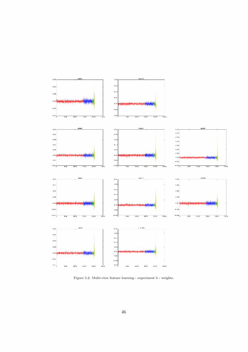
Figure 5.2: Multi-view feature learning - experiment b - weights.

46

Dataset: The dataset adopted in this experiment is STL-10 [10]. It is an

image dataset composed by colored picture of 96x96. It is a balanced

dataset and contains 500 samples per class for the training phase an

800 samples per class for the test phase. As it may be concluded from

the name, the number of target classes is 10. Since the size of the set

is very small, we decided to use a data augmentation technique, the

mirroring, obtaining a set that is double the size of the original one.

Moreover, 10% of the training data for the validation set was used,

thus we created a randomly a balanced subset composed of 50 images

per label.

Architecture Description: The architecture used to extract the features

was the following CNN:

Layer 1: It is a convolutional layer that takes as input a tensor of

3x96x96. It performs a convolution operation on a square of 5x5

and a max pooling operation on a square of 4x4. We decided to

use this large number to reduce drastically the number of features

extracted. It has 32 features map.

Layer 2: It is a convolutional layer that takes as input a tensor of

32x23x23. It performs a convolution operation on a square of

2x2 and a max pooling operation on a square 2x2. Now, that we

drastically reduced the number of features, we could use smaller

matrices to analyze the image better. This layer has 64 feature

maps.

Layer 3: It is a convolutional layer that takes as input a tensor of

64x11x11. It performs a convolution operation on a square of

2x2 and a max pooling operation on a square of 2x2. It has 128

feature maps.

Layer 4: It is a convolutional layer that takes as input a tensor of

128x5x5. It performs a convolution operation on a square of 2x2

and a max pooling operation on a square of 2x2. It has 256

feature maps.

Layer 5: It is a fully connected layer with 1024 hidden units. Each

of them takes as input the flatten results of the layer 4 that is

composed by 256x2x2 variables.

Layer 6: It is a logistic regression layer that has 10 units, one for each

label, and each takes as input the output of layer 5.

Moreover, the activation function used in all the layers was the ReLU

with the right initialization weights technique. As in experiment B,

47

Table 5.3: EXPERIMENT C - RESULTS

Method Accuracy

CNN 0.5195

MVL model 0.599

l2,1-norm model 0.47525

G1-norm model 0.5813

Logistic Regression 0.57475

on layer 5 and 6 we applied dropout as regularization technique. Ad-

ditionally, we used the validation dataset to control the performance

in order to avoid overfitting and pick the best model. For the learning

rate we used mini-batch gradient descent with momentum and learning

rate decay. The batch size adopted was 16 and the maximum number

of epochs was 200.

The results are presented in Table 5.3. We can observe that this time

even single view approach is able to surpass the baseline. However, the

MVL algorithm remains the one which earns more in terms of accuracy. It

is another proof that the previous layers may contain knowledge that is lost

during the learning procedure of the network.

As in previous experiments, we can print the weights in order to un-

derstand where the most significant features are and from which layer the

increase come from.

In Figure 5.3 we can observe the weights for each target class. There

are printed the weights for each label of the experimental evaluation that

has been made. In red, there are the weights for the feature extracted from

layer 1 (16928 features). In blue, there are the features extracted from layer

2 (7744 features). In green, there are the weights for the features extracted

from the layer 3 (3200 features). And in yellow, there are the features ex-

tracted from the layer 4 (1024 features) and in magenta, from the layer 5

(1024 features.). With a first glance we can note a contrast with the two

experiments described above. It is seen that the features extracted from the

last layers are less discriminative, their weights are around the zero. On

the other hand, the features extracted from first layers, the ones near the

input, are far more important and they have very wide range of values based

on the labels. A greater variance with different peaks may be observed in

this experiment. Moreover, with respect to previous cases, there are more

features set around the zero.

We think that this behavior is due to the following causes. First of all,

48

Figure 5.3: Multi-view feature learning - experiment c - weights.

49

a lot of features with the initial layers were extracted, so it is more likely

that there are some groups that are discriminative. Secondly, we performed

a “brutal” pooling in order to immediately decrease the number of features

and this could have influenced the behavior of the net. Neural networks are

very sophisticated and delicate models, so it is really hard to understand

properly what is going on, therefore, it is possible that the training was

stopped too early. As last consideration, we needed to underline the fact

that even a naive approach as Logistic Regresion on the concatenation of

the views outperforms the base CNN, so the strange behavior of the weights

may be caused, as it has just been said, by under-training of the ANN. How-

ever, this means that even if the training was not done properly, it is still

possible to obtain acceptable results by exploiting the informations from all

the previous layers to compensate the mistakes that we made in the training

phase.

5.4 Experiment D

After using famous internet datasets about VR, we have decided to adopt a

completely new one from a student of Politecnico di Milano. The set up of

this experiment is the following one:

Dataset: This dataset is extracted from a pipeline created by another stu-

dent of Politecnico di Milano for his thesis [39]. More precisely, the

problem addressed by the author is to automatically identify the digits

in a picture even in adverse condition (green light, noise etc). They

have created a tool that performs the following operations: first a cam-

era will capture the display of what we want to read, in this case it is

the display of a digital thermometer; second the system will automat-

ically split the images in sub-pictures where each of them will contain

a digit, and in the last stage there is the classification task. The final

goal of this work is the automatic reading of temperatures depicted in

digital displays of thermostats. We have taken the dataset produced

at the end second step in order to perform our experiment.

It is a coloured image dataset and each picture has a variable size.

It is composed by 11 classes, one per digit and the last class is the

noisy one, it means that it is not a digit or it is composed by two or

more ones, therefore we are not interested in it because our purpose is

to identify just single digit. It is composed by 4706 samples and the

majority class is the noisy one that is composed by 1798 instances.

We have resized the pictures to 3x20x20. If the image was too small

50

we have expanded it adding the color on the border, otherwise we have

shrink them. The transformation are made starting from the center of

the image.

In this case, we have adopted the 10 cross fold validation technique.

Each fold is stratified, so they have the same percentage of classes of

the original dataset, hence they are a good representation.

Architecture Description: The architecture used to extract the features

was the following CNN:

Layer 1: It is a convolutional layer that takes as input a tensor of

3x20x20. It performs a convolution operation on a square of 3x3

and a max pooling operation on a square of 2x2. We decided to

use this large number to reduce drastically the number of features

extracted. It has 64 features map.

Layer 2: It is a convolutional layer that takes as input a tensor of

64x9x9. It performs a convolution operation on a square of 2x2

and a max pooling operation on a square 2x2. Now, that we

drastically reduced the number of features, we could use smaller

matrices to analyze the image better. This layer has 128 feature

maps.

Layer 3: It is a convolutional layer that takes as input a tensor of

128x4x4. It performs a convolution operation on a square of 3x3

and a max pooling operation on a square of 2x2. It has 256

feature maps.

Layer 4: It is a fully connected layer with 64 hidden units. Each

of them takes as input the flatten results of the layer 4 that is

composed by 256x1x1 variables.

Layer 5: It is a logistic regression layer that has 11 units, one for each

label, and each takes as input the output of layer 4.

Moreover, the activation function used in all the layers was the ReLU

with the right initialization weights technique. As in experiment C

and B, on layer 4 and 5 we applied dropout as regularization tech-

nique. Additionally, in each run of the 10 cross fold validation, we

created from the 9 folds that we used as training set a validation set

to control the performance in order to avoid overfitting and pick the

best model. For the learning rate we used mini-batch gradient descent

with momentum and learning rate decay. The batch size adopted was

50 and the maximum number of epochs was 200.

51

Table 5.4: EXPERIMENT D - RESULTS

Method Accuracy

Majority Class 0.3821

CNN 81.34 ± 0.9532

MVL model 82.1534 ± 0.02423

l2,1-norm model 0.6080±0.02145

G1-norm model 0.8025± 0.00934

Logistic Regression 0.80359 ±0.0196889

The results are presented in Table 5.4. We can make the following obser-

vations: first of all, only the multi-view learning method is able to increase

the performance, however it is just a slightly increment (≈ 1). The second

and the most significant aspect is the decrease of the standard deviation

making the model more sound and reliable. It is another proof that in the

previous layers there are useful information that the network is not able to

extract by itself, but it is possible through a multi-view learning method.

As in previous experiments, we can print the weights in order to un-

derstand where the most significant features are and from which layer the

increase come from.

In Figure 5.4 we can observe the weights for each target class. There

are printed the weights for each label of the experimental evaluation that

has been made. In red, there are the weights for the feature extracted from

layer 1 (5184 features). In blue, there are the features extracted from layer

2 (2048 features). In green, there are the weights for the features extracted

from the layer 3 (256 features). And in yellow, there are the features ex-

tracted from the layer 4 (64 features). With a first glance we can note a

similar behaviour with respect the experiments A and B. Indeed, the fea-

tures extracted from the last layer are the more discriminative. Generally

speaking, their weights are bigger with respect the features extracted from

previous layers. However, with a more detailed investigation we can see that

it is a general trend, but in some cases (e.g. label 3 and 5) the features are

equally important. Moreover, we have some peak in the features extracted

from layer one or two suggesting that are more discriminative with respect

to the ones extracted from the last layer.

We can make our final reflection about the importance and the relations

between the features and the weights. In the future we can also analyse them

in order to acquire a better understanding. In this case, we have observed

that we can consider some features useless, their contribution is really small.

52

Figure 5.4: Multi-view feature learning - experiment d - weights.

53

The value of the weight is near the zero, consequently they can introduce

some noise. For this reason, for a future work, a proper solution is to in-

troduce and use new technique of features selection with the aim to reduce

this noisy behaviour. We can also try different regularization techniques.

5.5 Experiment E

For the last experiment of our research work we used the following set-ups.

Dataset: This time we created a small dataset from image-net.org that

is a collection of labelled colored pictures of different sizes. It is orga-

nized in an hierarchy based on WordNet where each node is a label and

the average number of pictures is 500. It is a very famous database for

labelled images and every year they host the ILSVRC, the most fa-

mous competition for image recognition. We gathered just five classes

in order to perform this experiment. The classes are: football player,

fish, eagle, guitar and fabric. Additionally, we can ensure that there

was no overlapping between different classes. In order to make a bal-

anced dataset we decided at priori to use 1000 images per label for the

training, and 100 per class for validation and test sets. No preprocess-

ing techniques were used, but since the pictures have different sizes

and standard ANN accept fixed input size, we decided to crop from

the center of the image a square, obtaining images with size 200x200.

Architecture Description: The architecture for the CNN was the follow-

ing one:

Layer 1: Convolutional layer that takes as input a tensor of 3x200x200.

It performs a convolution operation on a square of 5x5 and a max

pooling on a square of 2x2. It has 32 features maps.

Layer 2: Convolutional layer that takes as input a tensor of 32x98x98.

It performs a convolution operation on a square of 3x3 and a max

pooling on a square of 2x2. It has 64 features maps.

Layer 3: Convolutional layer that takes as input a tensor of 64x48x48.

It performs a convolution operation on a square of 3x3 and a max

pooling on a square of 2x2. It has 128 features maps.

Layer 4: Convolutional layer that takes as input a tensor of 128x23x23.

It performs a convolution operation on a square of 4x4 and a max

pooling on a square of 2x2. It has 256 features maps.

54

Table 5.5: EXPERIMENT E - RESULTS

Method Accuracy

CNN 0.431736

MVL model –

l2,1-norm model –

G1-norm model –

Logistic Regression –

Layer 5: Convolutional layer that takes as input a tensor of 256x10x10.

It performs a convolution operation on a square of 3x3 and a max

pooling on a square of 2x2. It has 256 features maps.

Layer 6: Fully connected hidden layer that has 2048 units and each

of them takes as input the flatten results of the convolutional

layer 5 that has 256x4x4 variables.

Layer 7: Logistic regression layers that performs the prediction, there-

fore, it has 5 units and each of them takes as input the 2048

outputs of Layer 6.

As above, the activation function used for all the layers was the ReLU.

Additionally, the layer 6 and 7 implemented the dropout technique.

For the training stage, we adopted mini-batch gradient descent with

the addition of momentum and decay learning rate. The batch size

was 16 and the maximum number of epochs was 200.

We reported the results in Table 5.5. As it can be seen, no results are

shown because all the algorithms run out of memory on our machine (16Gb

RAM). With this experiments our intention was to show one of the limits

of this approach. The problem is that we multiplied the number of hidden

unites of the network for the size of the dataset, and this is requested just

to load the new training dataset.

We can do quick calculation with this example. We extracted: 307328

features from the first layer, 147456 features from the second one, 67712

features from the third layer, 25600 from the fourth, 4096 from the fifth and

2048 from the sixth layer. If we sum all the features, we have a total number

of 554240 and if we use 8 bytes (64 bit) for each of them, in order to not

lose precision, we will need ≈ 4Mb for each training example. So just for a

training dataset of 5000 samples, as in our case, we would need 20Gb just to

load the dataset in the memory. Thus, it is not feasible to run the proposed

approach with any algorithm we have proposed in this work.

55

So, with this experiment we want to point out a general problem that can

occur with this kind of approach. The number of features that we extract

per each layer can explode very easily, especially with CNN since we are

working with volume data. This may be a problem as it is true that with

more features we will generally have a better performance, but we will also

need more memory in order to manage all these information properly.

We are not going to solve this problem, however big data technique can

help to deal with it. Our aim was to underline it as there is no such a thing as

a free lunch. The method proposed has both advantages and disadvantages,

our objective is to show a new way of thinking and working with ANNs to

the community.

56

Chapter 6

Conclusion

In this work, we have introduced a novel way to look and work with ANNs

that, for the best of my knowledge, no previous works have dealt with.

The proposed research try to extract information from all the previous

layers of a ANN in order to increase the performance. The intuition was

born from the following idea: during the training stage there is no constraint

on the weights of the network, the only rule they follow is to minimize the

error rate in the last layer. This means that, if we consider each hidden

units as a feature, there may be a set of features more discriminative than

the last ones.Consequently, they can be of help for the prediction task. This

may happen because with back-propagation technique we do not force any

constraints to the weights and what is more important, it is not really clear

what is going on in the ANN. Therefore, we have proposed a combination

of two known techniques with the aim of studying this behaviour and find

out if it is possible to decrease the error rate. The framework adopted is a

two phase model. In the first stage there is a traditional ANN, for our case

study we have used CNNs. In the second stage a MVL algorithm has been

used.

We have thought that a MVL algorithm was more suitable for the follow-

ing reasons. Each layer of the ANN can be seen as a different latent-space

and the weights are the parameters for the transformation from a space to

another. In this different space the notion of similarity and distance are

different and at priori there is no one better than another. Therefore, it

may be helpful just for some specific classes. The same concepts may be

found in MKL, one family of algorithms of MVL, where different kernels

are combined with the purpose of increasing the performance. Therefore,

each layer can be seen as a view and we want to combine the features from

these different views with the MVL algorithm, what has been explained in

57

the above chapters.

In the experiment section we have performed different analysis with vari-

ous kind of architectures and datasets. We have showed that there are infor-

mation that are unexploited in previous layers and by printing the weights

of the algorithm we can observe it more easily. It can be claimed that there

is a clear benefit in the usage of the information of the previous layers.

However, there is not such a thing as free lunch. In all our case studies

we were able to increase the performance, however in the last experiment we

have faced a big problem. By using DNN we can extract a tons of features

that will require a lot of computational power to be processed and ordinary

methods will not manage it properly. We do not investigate it, but some

big data technique that splits the data and then combine the various results

can help with this aspect.

In the end, we think that our research shows some interesting behaviour

of ANNs. We want to underline that we do not want to compare ourselves

to state of the art techniques. Our purpose is to show that there is a clear

advantage of using features from previous layers, but doing it properly is

not an easy task.

Our goal is to show to the community that there are advantages of using

information from previous layers.

We hope that this exploration work will be an incentive and will be a

start point for new interesting research on this aspects.

58

Bibliography

[1] Frederic Bastien, Pascal Lamblin, Razvan Pascanu, James Bergstra,

Ian J. Goodfellow, Arnaud Bergeron, Nicolas Bouchard, and Yoshua

Bengio. Theano: new features and speed improvements. Deep Learning

and Unsupervised Feature Learning NIPS 2012 Workshop, 2012.

[2] Mikhail Belkin, Partha Niyogi, and Vikas Sindhwani. Manifold regular-

ization: A geometric framework for learning from labeled and unlabeled

examples. The Journal of Machine Learning Research, 7:2399–2434,

2006.

[3] Yoshua Bengio. Learning deep architectures for ai. Foundations and

trends R© in Machine Learning, 2(1):1–127, 2009.

[4] James Bergstra, Olivier Breuleux, Frederic Bastien, Pascal Lamblin,

Razvan Pascanu, Guillaume Desjardins, Joseph Turian, David Warde-

Farley, and Yoshua Bengio. Theano: a CPU and GPU math expression

compiler. In Proceedings of the Python for Scientific Computing Con-

ference (SciPy), June 2010. Oral Presentation.

[5] Avrim Blum and Tom Mitchell. Combining labeled and unlabeled data

with co-training. In Proceedings of the eleventh annual conference on

Computational learning theory, pages 92–100. ACM, 1998.

[6] Ulf Brefeld, Christoph Buscher, and Tobias Scheffer. Multi-view dis-

criminative sequential learning. In Machine Learning: ECML 2005,

pages 60–71. Springer, 2005.

[7] Soumen Chakrabarti, Martin Ester, Usama Fayyad, Johannes Gehrke,

Jiawei Han, Shinichi Morishita, Gregory Piatetsky-Shapiro, and Wei

Wang. Data mining curriculum: A proposal (version 1.0). Intensive

Working Group of ACM SIGKDD Curriculum Committee, 2006.

[8] Minmin Chen, Yixin Chen, and Kilian Q Weinberger. Automatic fea-

ture decomposition for single view co-training. In Proceedings of the

59

28th International Conference on Machine Learning (ICML-11), pages

953–960, 2011.

[9] C Christoudias, Raquel Urtasun, and Trevor Darrell. Multi-view

learning in the presence of view disagreement. arXiv preprint

arXiv:1206.3242, 2012.

[10] Adam Coates, Andrew Y Ng, and Honglak Lee. An analysis of single-

layer networks in unsupervised feature learning. In International con-

ference on artificial intelligence and statistics, pages 215–223, 2011.

[11] Ronald R Coifman, Stephane Lafon, Ann B Lee, Mauro Maggioni, Boaz

Nadler, Frederick Warner, and Steven W Zucker. Geometric diffusions

as a tool for harmonic analysis and structure definition of data: Dif-

fusion maps. Proceedings of the National Academy of Sciences of the

United States of America, 102(21):7426–7431, 2005.

[12] Balazs Csanad Csaji. Approximation with artificial neural networks.

Faculty of Sciences, Etvs Lornd University, Hungary, 24:48, 2001.

[13] George Cybenko. Approximation by superpositions of a sigmoidal func-

tion. Mathematics of control, signals and systems, 2(4):303–314, 1989.

[14] Sanjoy Dasgupta, Michael L Littman, and David McAllester. Pac gen-

eralization bounds for co-training. Advances in neural information pro-

cessing systems, 1:375–382, 2002.

[15] Radek Erban, Thomas A Frewen, Xiao Wang, Timothy C Elston,

Ronald Coifman, Boaz Nadler, and Ioannis G Kevrekidis. Variable-free

exploration of stochastic models: a gene regulatory network example.

The Journal of chemical physics, 126(15):155103, 2007.

[16] Kunihiko Fukushima. Neocognitron: A self-organizing neural network

model for a mechanism of pattern recognition unaffected by shift in

position. Biological cybernetics, 36(4):193–202, 1980.

[17] Xavier Glorot and Yoshua Bengio. Understanding the difficulty of train-

ing deep feedforward neural networks. In International conference on

artificial intelligence and statistics, pages 249–256, 2010.

[18] Ian J Goodfellow, David Warde-Farley, Mehdi Mirza, Aaron Courville,

and Yoshua Bengio. Maxout networks. arXiv preprint arXiv:1302.4389,

2013.

60

[19] Benjamin Graham. Fractional max-pooling. arXiv preprint

arXiv:1412.6071, 2014.

[20] Kaiming He, Xiangyu Zhang, Shaoqing Ren, and Jian Sun. Deep resid-

ual learning for image recognition. arXiv preprint arXiv:1512.03385,

2015.

[21] Kaiming He, Xiangyu Zhang, Shaoqing Ren, and Jian Sun. Delving

deep into rectifiers: Surpassing human-level performance on imagenet

classification. In Proceedings of the IEEE International Conference on

Computer Vision, pages 1026–1034, 2015.

[22] Geoffrey E Hinton. Learning multiple layers of representation. Trends

in cognitive sciences, 11(10):428–434, 2007.

[23] Geoffrey E Hinton, Nitish Srivastava, Alex Krizhevsky, Ilya Sutskever,

and Ruslan R Salakhutdinov. Improving neural networks by preventing

co-adaptation of feature detectors. arXiv preprint arXiv:1207.0580,

2012.

[24] David H Hubel and Torsten N Wiesel. Receptive fields and func-

tional architecture of monkey striate cortex. The Journal of physiology,

195(1):215–243, 1968.

[25] Sergey Ioffe and Christian Szegedy. Batch normalization: Accelerat-

ing deep network training by reducing internal covariate shift. arXiv

preprint arXiv:1502.03167, 2015.

[26] Alex Krizhevsky and Geoffrey Hinton. Learning multiple layers of fea-

tures from tiny images, 2009.

[27] Alex Krizhevsky, Ilya Sutskever, and Geoffrey E Hinton. Imagenet

classification with deep convolutional neural networks. In Advances in

neural information processing systems, pages 1097–1105, 2012.

[28] Yann LeCun, Leon Bottou, Yoshua Bengio, and Patrick Haffner.

Gradient-based learning applied to document recognition. Proceedings

of the IEEE, 86(11):2278–2324, 1998.

[29] Andrew L Maas, Awni Y Hannun, and Andrew Y Ng. Rectifier non-

linearities improve neural network acoustic models. In Proc. ICML,

volume 30, page 1, 2013.

61

[30] Warren S McCulloch and Walter Pitts. A logical calculus of the ideas

immanent in nervous activity. The bulletin of mathematical biophysics,

5(4):115–133, 1943.

[31] Jesus Mena. Machine learning forensics for law enforcement, security,

and intelligence. CRC Press, 2011.

[32] Marvin Minsky and Seymour Papert. Perceptron: an introduction to

computational geometry. The MIT Press, Cambridge, expanded edition,

19(88):2, 1969.

[33] Ion Muslea, Steven Minton, and Craig A Knoblock. Active+ semi-

supervised learning= robust multi-view learning. In ICML, volume 2,

pages 435–442, 2002.

[34] Yurii Nesterov. Introductory lectures on convex optimization: A basic

course, volume 87. Springer Science & Business Media, 2013.

[35] John Nickolls, Ian Buck, Michael Garland, and Kevin Skadron. Scalable

parallel programming with cuda. Queue, 6(2):40–53, 2008.

[36] Guillaume Obozinski, Ben Taskar, and Michael I Jordan. Joint co-

variate selection and joint subspace selection for multiple classification

problems. Statistics and Computing, 20(2):231–252, 2010.

[37] Fabian Pedregosa, Gael Varoquaux, Alexandre Gramfort, Vincent

Michel, Bertrand Thirion, Olivier Grisel, Mathieu Blondel, Peter Pret-

tenhofer, Ron Weiss, Vincent Dubourg, et al. Scikit-learn: Ma-

chine learning in python. The Journal of Machine Learning Research,

12:2825–2830, 2011.

[38] Khalid Raza. Application of data mining in bioinformatics. arXiv

preprint arXiv:1205.1125, 2012.

[39] GIOVANNI RECUPERO. Deep learning for camera-based temperature

recognition from digital displays. 2016.

[40] Frank Rosenblatt. The perceptron: a probabilistic model for infor-

mation storage and organization in the brain. Psychological review,

65(6):386, 1958.

[41] Jurgen Schmidhuber. Deep learning in neural networks: An overview.

Neural Networks, 61:85–117, 2015.

62

[42] Nitish Srivastava, Geoffrey Hinton, Alex Krizhevsky, Ilya Sutskever,

and Ruslan Salakhutdinov. Dropout: A simple way to prevent neural

networks from overfitting. The Journal of Machine Learning Research,

15(1):1929–1958, 2014.

[43] Ilya Sutskever, James Martens, George Dahl, and Geoffrey Hinton. On

the importance of initialization and momentum in deep learning. In

Proceedings of the 30th international conference on machine learning

(ICML-13), pages 1139–1147, 2013.

[44] Christian Szegedy, Wei Liu, Yangqing Jia, Pierre Sermanet, Scott Reed,

Dragomir Anguelov, Dumitru Erhan, Vincent Vanhoucke, and Andrew

Rabinovich. Going deeper with convolutions. In Proceedings of the

IEEE Conference on Computer Vision and Pattern Recognition, pages

1–9, 2015.

[45] Stefan Van Der Walt, S Chris Colbert, and Gael Varoquaux. The numpy

array: a structure for efficient numerical computation. Computing in

Science & Engineering, 13(2):22–30, 2011.

[46] Hua Wang, Feiping Nie, and Heng Huang. Multi-view clustering and

feature learning via structured sparsity. In Proceedings of the 30th Inter-

national Conference on Machine Learning (ICML-13), pages 352–360,

2013.

[47] Wei Wang and Zhi-Hua Zhou. Analyzing co-training style algorithms.

In Machine Learning: ECML 2007, pages 454–465. Springer, 2007.

[48] Zhe Wang, Songcan Chen, and Daqi Gao. A novel multi-view learning

developed from single-view patterns. Pattern Recognition, 44(10):2395–

2413, 2011.

[49] Chang Xu, Dacheng Tao, and Chao Xu. A survey on multi-view learn-

ing. arXiv preprint arXiv:1304.5634, 2013.

[50] Jieping Ye, Zheng Zhao, and Mingrui Wu. Discriminative k-means for

clustering. In Advances in neural information processing systems, pages

1649–1656, 2008.

[51] Guangchao Yuan, Pradeep K Murukannaiah, Zhe Zhang, and Munin-

dar P Singh. Exploiting sentiment homophily for link prediction. In

Proceedings of the 8th ACM Conference on Recommender systems,

pages 17–24. ACM, 2014.

63

[52] Ming Yuan and Yi Lin. Model selection and estimation in regression

with grouped variables. Journal of the Royal Statistical Society: Series

B (Statistical Methodology), 68(1):49–67, 2006.

64