
Multi-unit auctions & exchanges (multiple indistinguishable units of one item for sale) Tuomas...
26
Multi-unit auctions & exchanges (multiple indistinguishable units of one item for sale) Tuomas Sandholm Computer Science Department Carnegie Mellon University
-
date post
20-Dec-2015 -
Category
Documents
-
view
216 -
download
1
Transcript of Multi-unit auctions & exchanges (multiple indistinguishable units of one item for sale) Tuomas...

Multi-unit auctions & exchanges
(multiple indistinguishable units of one item for sale)
Tuomas Sandholm
Computer Science Department Carnegie Mellon University

Auctions with multiple indistinguishable units for sale
• Examples– IBM stocks– Barrels of oil– Pork bellies– Trans-Atlantic backbone bandwidth from NYC to Paris– …

Bidding languages and expressiveness
• These bidding languages were introduced for combinatorial auctions, but also apply to multi-unit auctions– OR [default; Sandholm 99]– XOR [Sandholm 99]– OR-of-XORs [Sandholm 99]– XOR-of-ORs [Nisan 00]– OR* [Fujishima et al. 99, Nisan 00]– Recursive logical bidding languages [Boutilier & Hoos 01]
• In multi-unit setting, can also use price-quantity curve bids

Screenshot from eMediator[Sandholm AGENTS-00, Computational Intelligence 02]

Multi-unit auctions: pricing rules• Auctioning multiple indistinguishable units of an item• Naive generalization of the Vickrey auction: uniform price auction
– If there are m units for sale, the highest m bids win, and each bid pays the m+1st highest price
– Downside with multi-unit demand: Demand reduction lie [Crampton&Ausubel 96]:
• m=5• Agent 1 values getting her first unit at $9, and getting a second unit
is worth $7 to her• Others have placed bids $2, $6, $8, $10, and $14• If agent 1 submits one bid at $9 and one at $7, she gets both items,
and pays 2 x $6 = $12. Her utility is $9 + $7 - $12 = $4• If agent 1 only submits one bid for $9, she will get one item, and pay
$2. Her utility is $9-$2=$7• Incentive compatible mechanism that is Pareto efficient and ex post
individually rational – Clarke tax. Agent i pays a-b
• b is the others’ sum of winning bids• a is the others’ sum of winning bids had i not participated
– I.e., if i wins n items, he pays the prices of the n highest losing bids– What about revenue (if market is competitive)?

General case of efficiency under diminishing values
• VCG has efficient equilibrium. What about other mechanisms?
• Model: xik is i’s signal (i.e., value) for his k’th unit.
– Signals are drawn iid and support has no gaps– Assume diminishing values
• Prop. [13.3 in Krishna book]. An equilibrium of a multi-unit auction where the highest m bids win is efficient iff the bidding strategies are separable across units and bidders, i.e., βi
k(xi)= β(xi
k)
– Reasoning: efficiency requires xik > xi
r iff βik(xi) > βi
r(xi)• So, i’s bid on some unit cannot depend on i’s signal on another unit• And symmetry across bidders needed for same reason as in 1-object case

Revenue equivalence theorem (which we proved before) applies
to multi-unit auctions
• Again assumes that – payoffs are same at some zero type, and – the allocation rule is the same
• Here it becomes a powerful tool for comparing expected revenues
Multi-unit auctions: Clearing complexity
[Sandholm & Suri IJCAI-01]


In all of the curves together


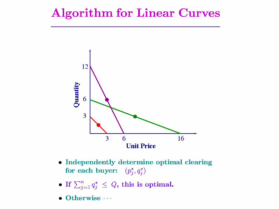

∑


Multi-unit reverse auctions with supply curves
• Same complexity results apply as in auctions– O(#pieces log #pieces) in nondiscriminatory case
with piecewise linear supply curves– NP-complete in discriminatory case with
piecewise linear supply curves– O(#agents log #agents) in discriminatory case with
linear supply curves
Multi-unit exchanges• Multiple buyers, multiple sellers, multiple units for sale• By Myerson-Satterthwaite thrm, even in 1-unit case cannot obtain all of
• Pareto efficiency• Budget balance• Individual rationality (participation)

Supply/demand curve bids
profit = amounts paid by bidders – amounts paid to sellersCan be divided between buyers, sellers & market maker
Unit price
Quantity Aggregate supply Aggregate demand
One price for everyone (“classic partial equilibrium”):profit = 0
One price for sellers, one for buyers ( nondiscriminatory pricing ): profit > 0
profit
psell pbuy

Nondiscriminatory vs. discriminatory pricing
Unit price
Quantity
Supply of agent 1
Aggregate demand
Supply of agent 2
One price for sellers, one for buyers( nondiscriminatory pricing ): profit > 0
psell pbuy
One price for each agent ( discriminatory pricing ): greater profit
p1sell
pbuyp2sell

Shape of supply/demand curves
• Piecewise linear curve can approximate any curve• Assume
– Each buyer’s demand curve is downward sloping– Each seller’s supply curve is upward sloping– Otherwise absurd result can occur
• Aggregate curves might not be monotonic• Even individuals’ curves might not be continuous

Pricing scheme has implications on time complexity of clearing
• Piecewise linear curves (not necessarily continuous) can approximate any curve• Clearing objective: maximize profit• Thrm. Nondiscriminatory clearing with piecewise linear supply/demand: O(p log p)
– p = total number of pieces in the curves
• Thrm. Discriminatory clearing with piecewise linear supply/demand: NP-complete• Thrm. Discriminatory clearing with linear supply/demand: O(a log a)
– a = number of agents
• These results apply to auctions, reverse auctions, and exchanges• So, there is an inherent tradeoff between profit and computational complexity – even
without worrying about incentives


![Constraint Satisfaction Problems Tuomas Sandholm Carnegie Mellon University Computer Science Department [Read Chapter 6 of Russell & Norvig]](https://static.fdocuments.in/doc/165x107/56649dd45503460f94acc529/constraint-satisfaction-problems-tuomas-sandholm-carnegie-mellon-university.jpg)


