
Multi-fluid Plasma Modelling can only say that I hope postgraduate studies will be as rewarding an...
85
Multi-fluid Plasma Modelling Graham Russell Dennis A thesis submitted in partial fulfilment of the requirements for the degree of Bachelor of Philosophy with Honours at The Australian National University November 2005
Transcript of Multi-fluid Plasma Modelling can only say that I hope postgraduate studies will be as rewarding an...

Multi-fluid Plasma Modelling
Graham Russell Dennis
A thesis submitted in partial fulfilment of the requirements forthe degree of Bachelor of Philosophy with Honours
at The Australian National University
November 2005

ii
Declaration
This thesis is an account of research undertaken under the supervision of Dr. Matthew Holebetween February 2005 and November 2005 at The Department of Theoretical Physics,Research School of Physical Sciences and Engineering, The Australian National University,Canberra, Australia.
Except where acknowledged in the customary manner, the material presented in thisthesis is, to the best of my knowledge, original and has not been submitted in whole orpart for a degree in any university.
Graham Russell DennisNovember 2005
iii

iv
Acknowledgements
It’s been a long year, but has most certainly been both enjoyable and enlightening. Thiswould not have been possible without the constant guidance and support of my supervisor,Dr. Matthew Hole.
Along the way, there have been many people who have helped out, and deserve mention.I’d like to thank my parents for their love and support, and also for taking the time tofly down from Mount Isa for my 21st Birthday this year. I also wish to acknowledge theassistance given by Luca Guazzotto from the University of Rochester in helping us to getFLOW to compile and run, and also answering questions about the code throughout theyear.
To my many proof-readers, I am incredibly grateful for your assistance: Andrew,Andrew, Anthony, Emma, Erin, John, Paul, Peter, Mum & Dad.
To the students of the basement of RSPhysSE, all I can say is thanks for providingdistractions during my many hours over at the Research School. Particularly my variousoffice-mates throughout the year, including Farzand, Emma, Andrew, Sangeetha, and theever-elusive Norman.
I would also like to thank the people at Ursies for many lively games of pool andping-pong, and continually reminding me that I need to get back to work.
I can only say that I hope postgraduate studies will be as rewarding an experience asHonours has been.
v

vi

Abstract
Contemporary plasma fusion experiments use significant power injection for plasma heat-ing. The injected power selectively heats only part of the plasma, which then transfers itsenergy to the rest of the plasma through collisions. Continuous power injection gives riseto a dynamic equilibrium whereby part of the plasma has a higher energy than the bulkof the plasma. Current plasma fluid treatments assume that the velocity distribution ofeach particle species is described by a Maxwell-Boltzmann distribution function, and somay not be accurate for plasmas with a significant energetic component.
A new method of modelling toroidally-symmetric plasma equilibria is derived in thisthesis: multi-fluid plasma modelling. In this model, the non-Maxwellian plasma is decom-posed into an arbitrary number of energy-resolved fluids. Each fluid is charge-neutral, canhave arbitrary rotation, and is described by a Maxwellian distribution function.
To investigate the model numerically, it is implemented as a modification to an existingsingle-fluid plasma equilibrium code. The modified code is then used to investigate theeffect of an energetic component on the plasma equilibrium. We find that the influence ofthe energetic component can be significant if it has large toroidal flow (or flow-shear). Theplasma equilibrium is, however, relatively robust to variations in the energetic component’storoidal flow and pressure profiles.
vii

viii

Contents
Declaration iii
Acknowledgements v
Abstract vii
1 Introduction 11.1 Overview . . . . . . . . . . . . . . . . . . . . . . . . . . . . . . . . . . . . . 11.2 Existing Modelling Techniques and their Limitations . . . . . . . . . . . . . 11.3 Multi-fluid Modelling . . . . . . . . . . . . . . . . . . . . . . . . . . . . . . . 31.4 Thesis Outline . . . . . . . . . . . . . . . . . . . . . . . . . . . . . . . . . . 4
2 Tokamak Plasma Physics 52.1 Plasmas & Fusion . . . . . . . . . . . . . . . . . . . . . . . . . . . . . . . . 52.2 A Brief History of the Tokamak . . . . . . . . . . . . . . . . . . . . . . . . . 62.3 Non-thermalised Plasmas . . . . . . . . . . . . . . . . . . . . . . . . . . . . 7
2.3.1 Ohmic Heating . . . . . . . . . . . . . . . . . . . . . . . . . . . . . . 72.3.2 Radio Frequency Heating . . . . . . . . . . . . . . . . . . . . . . . . 82.3.3 Neutral Beam Heating . . . . . . . . . . . . . . . . . . . . . . . . . . 10
2.4 Theoretical Descriptions of Tokamak Equilibria . . . . . . . . . . . . . . . . 112.4.1 The Vlasov & Fokker-Planck Equations . . . . . . . . . . . . . . . . 112.4.2 The Two-fluid Model . . . . . . . . . . . . . . . . . . . . . . . . . . . 112.4.3 The Ideal MHD Model . . . . . . . . . . . . . . . . . . . . . . . . . . 122.4.4 The Grad-Shafranov Equation . . . . . . . . . . . . . . . . . . . . . 132.4.5 Generalisations of the Grad-Shafranov Equation . . . . . . . . . . . 142.4.6 Multi-fluid Models . . . . . . . . . . . . . . . . . . . . . . . . . . . . 14
2.5 Plasma Equilibrium Solutions with Flow . . . . . . . . . . . . . . . . . . . . 152.5.1 Analytical Solutions . . . . . . . . . . . . . . . . . . . . . . . . . . . 152.5.2 Numerical Solutions . . . . . . . . . . . . . . . . . . . . . . . . . . . 15
3 A Multi-fluid Force-balance Equation 173.1 Overview . . . . . . . . . . . . . . . . . . . . . . . . . . . . . . . . . . . . . 173.2 A Multiple Quasi-neutral Fluid Model . . . . . . . . . . . . . . . . . . . . . 183.3 Flux Functions for Velocity . . . . . . . . . . . . . . . . . . . . . . . . . . . 203.4 The Fluid Force-balance Equation . . . . . . . . . . . . . . . . . . . . . . . 213.5 Flux Functions from the Force-balance Equation . . . . . . . . . . . . . . . 233.6 The Generalised Grad-Shafranov Equation . . . . . . . . . . . . . . . . . . . 263.7 Reductions to Previous Results . . . . . . . . . . . . . . . . . . . . . . . . . 28
3.7.1 Reduction to Guazzotto et al. . . . . . . . . . . . . . . . . . . . . . . 283.7.2 Reduction to McClements and Thyagaraja . . . . . . . . . . . . . . 29
3.8 Summary of the Derivation . . . . . . . . . . . . . . . . . . . . . . . . . . . 30
ix

x Contents
4 Calculating Solutions of the Multi-fluid Grad-Shafranov Equation 314.1 Numerical Methods for Solving PDE’s . . . . . . . . . . . . . . . . . . . . . 31
4.1.1 Finite-difference Approximation . . . . . . . . . . . . . . . . . . . . . 314.1.2 Newton-Gauss-Seidel Method . . . . . . . . . . . . . . . . . . . . . . 334.1.3 Red-Black Ordering . . . . . . . . . . . . . . . . . . . . . . . . . . . 334.1.4 Multigrid Method . . . . . . . . . . . . . . . . . . . . . . . . . . . . 34
4.2 The FLOW Code . . . . . . . . . . . . . . . . . . . . . . . . . . . . . . . . . 354.2.1 Overview of the Structure of FLOW . . . . . . . . . . . . . . . . . . 364.2.2 Solving the Bernoulli Equation . . . . . . . . . . . . . . . . . . . . . 36
4.3 Structural Changes Required in FLOW . . . . . . . . . . . . . . . . . . . . 394.4 Parameterising the Solution . . . . . . . . . . . . . . . . . . . . . . . . . . . 404.5 Scaling Relationships . . . . . . . . . . . . . . . . . . . . . . . . . . . . . . . 434.6 CHEASE Benchmark . . . . . . . . . . . . . . . . . . . . . . . . . . . . . . . 444.7 Multi-fluid Benchmark . . . . . . . . . . . . . . . . . . . . . . . . . . . . . . 46
5 Numerical Scans 495.1 Plasma Performance Measures . . . . . . . . . . . . . . . . . . . . . . . . . 49
5.1.1 Plasma β . . . . . . . . . . . . . . . . . . . . . . . . . . . . . . . . . 495.1.2 Shafranov Shift, ∆S . . . . . . . . . . . . . . . . . . . . . . . . . . . 505.1.3 Safety Factor, q . . . . . . . . . . . . . . . . . . . . . . . . . . . . . . 50
5.2 Physics Studies . . . . . . . . . . . . . . . . . . . . . . . . . . . . . . . . . . 515.2.1 Profile Parameterisations . . . . . . . . . . . . . . . . . . . . . . . . 515.2.2 Constraints . . . . . . . . . . . . . . . . . . . . . . . . . . . . . . . . 515.2.3 Scan of Menergetic,φ,max . . . . . . . . . . . . . . . . . . . . . . . . . . 525.2.4 Scan of Menergetic,θ,max . . . . . . . . . . . . . . . . . . . . . . . . . . 575.2.5 Scan of Penergetic,centre . . . . . . . . . . . . . . . . . . . . . . . . . . 60
5.3 Equilibrium Sensitivity to Profile Variations . . . . . . . . . . . . . . . . . . 625.3.1 Profile Parameterisations . . . . . . . . . . . . . . . . . . . . . . . . 635.3.2 Constraints . . . . . . . . . . . . . . . . . . . . . . . . . . . . . . . . 635.3.3 Method . . . . . . . . . . . . . . . . . . . . . . . . . . . . . . . . . . 645.3.4 Results & Discussion . . . . . . . . . . . . . . . . . . . . . . . . . . . 65
6 Conclusion 696.1 Future Directions . . . . . . . . . . . . . . . . . . . . . . . . . . . . . . . . . 70
Bibliography 73

Chapter 1
Introduction
1.1 Overview
Since the pioneering work of Einstein, who recognised that matter and energy are related,harnessing nuclear power for peaceful purposes has been identified as a long-term sciencegoal. Active research into harnessing fusion — the process that powers the Sun and thestars — commenced in earnest following the Second World War.
Although a laudable aim, achieving net power output from a fusion reaction is a verydifficult problem. For fusion to occur, two positively charged nuclei must come closeenough for the attractive strong nuclear force to overcome the repulsive Coulomb force.Moreover, the fusion reactants must be confined at a sufficiently high density, and for asufficient length of time, for enough energy to be released to exceed the energy requiredto initiate the reaction.
To overcome the Coulomb barrier, the fusion reactants must be heated to temperaturesaround 108 K, or 10 times that of the core of the Sun. At these extreme temperatures,the reactants will be completely ionised, i.e. in the plasma state. Because of the chargeseparation caused by ionisation, a plasma exhibits collective behaviour caused by thelong-range interactions between the charged particles and the electromagnetic fields theparticles create. These electromagnetic fields can be manipulated externally, enablingsome degree of control over the plasma’s behaviour.
The tokamak [1, 2] is one experimental device designed to take advantage of the con-trol provided by external magnetic fields to confine the plasma within a certain volume,physically isolating it from the containing vessel (see Figure 1.1 for a schematic of a typ-ical tokamak design). Using this method, the plasma can be thermally insulated fromits environment. This thesis investigates a new method of modelling the equilibrium oftokamak plasmas.
1.2 Existing Modelling Techniques and their Limitations
A plasma is a complex system because the motion of the particles and the behaviour of theelectromagnetic fields are interdependent. Understanding and modelling the dynamics ofsuch systems is a challenging task. In addition to the fundamental value of such research,this knowledge can also be used to advance the long-term goal of fusion power.
There are a number of different approaches to modelling plasma behaviour, but theycan be broadly divided into two classes: microscopic modelling and macroscopic modelling.Microscopic modelling considers the plasma behaviour on the scale length of the particles’orbits of the magnetic field lines, defined as the Larmor radius (∼10−3m for ions, and∼10−5m for electrons in a tokamak plasma). This type of modelling is generally used for
1

2 Introduction
Central solenoid magnet
Poloidal-field magnet
Toroidal-field magnet
Figure 1.1: A cutaway of a typical tokamak design.
plasmas where the Larmor radius is a significant fraction of the size of the plasma. Forplasmas where the Larmor radius is a small fraction of the size of the plasma, microscopicmodelling becomes computationally difficult due to the large amount of detail in the model.
The other class of plasma models are the macroscopic models. These models considerthe plasma behaviour on the scale length of the total plasma size by averaging, in somesense, over the smaller-scale behaviour. However, macroscopic modelling can, when ap-plied to some systems, lead to the loss of vital physical effects, and so must be appliedwith caution.
The most direct form of microscopic modelling would be to model the interactionsbetween the electromagnetic fields and each individual particle in the plasma. A moresophisticated version of this idea is known as the particle-in-cell method [3]. In thismethod, the plasma is modelled as containing a large number of conglomerate particles,each of which represents many real particles. The pressure and electromagnetic fields arecalculated on a coarser grid of cells from the positions and velocities of the conglomerateparticles. This information is then used to evolve the positions and velocities of theseparticles. As the number of particles in the plasma increases, the computational demandsof the particle-in-cell technique can become too great, and eventually another form ofmodelling is needed.
Kinetic modelling is a form of microscopic modelling where the probability distributionfunction of the particles’ velocities is evolved about an equilibrium probability distributionfunction by a variational method. This variational method is known as the δf method [4]because the velocity distribution function of each plasma species is fully described by the7-dimensional function f(x,v, t), and it is a variation δf of f that is evolved. Althoughthis method is computationally more feasible than the particle-in-cell method for largeplasmas, it is still difficult because of the high dimensionality of the problem.
To further simplify the problem, other models make some additional physical assump-

§1.3 Multi-fluid Modelling 3
tions about the plasma’s behaviour. In the two-fluid treatment, the ions and electrons inthe plasma are modelled as fluids, each described by a number of macroscopic parame-ters including density, pressure and mean fluid velocity at each point in the plasma. Theevolution of these quantities is described by a set of equations that are obtained by aver-aging over the equations that describe the kinetic model. A difficulty arises in that thisaveraging process does not lead to a closed system of equations.
To close the system of equations, a further approximation is needed to simplify thehigher-order effects of the plasma. Typically, this approximation includes the assumptionthat at each point in the plasma, the velocity distribution of the particles is describedby the Maxwell-Boltzmann distribution, a statistical steady-state. As a result, a singletemperature can be defined at each point in the plasma that describes the shape of thevelocity distribution function at that point. In more sophisticated models, some levelof anisotropy is permitted, and two temperatures are used to describe the shape of thevelocity distribution. One of these temperatures describes the component of the velocitydistribution parallel to the local magnetic field, and the other describes the component ofthe velocity distribution perpendicular to the local magnetic field.
Magnetohydrodynamics (MHD) is a further simplification of the two-fluid model inwhich the two fluids are combined as a single fluid. The approximation made in the MHDmodel is to neglect the mass of the electrons compared to the ion mass, and the electronpressure compared to that of the ions. This approximation is satisfied for the plasmasused in contemporary tokamak fusion experiments.
In experimental fusion plasmas, it is often the case that the velocity distribution of theparticles does not conform to the Maxwell-Boltzmann distribution; this is due to externalheating, used both to compensate for energy losses, and to increase the plasma tempera-ture. Often, the heating mechanisms heat only particles within a certain velocity range.Energy is then transferred from the component of the plasma resonant with the heatingmechanism to the rest of the plasma through collisions. If the heating process were ceased,the plasma would eventually return to a Maxwellian distribution function. However, ifthe heating process is continuous, as is the case in modern tokamak experiments, then adynamic equilibrium arises in which energy is transferred into the resonant component ofthe distribution function at the same rate as it looses energy to the bulk of the plasma.In this dynamic equilibrium, the high-energy component of the plasma can be seen as astationary ‘bump’ in the tail of the velocity distribution function of the whole plasma, asshown in Figure 1.2. For plasmas with a significant amount of heating, this ‘bump’ cancause the distribution function to be highly non-Maxwellian, and so a temperature cannotbe defined. It is not currently known how much of an effect neglecting the contribution ofa high-energy component of the distribution function has upon the fluid models previouslydiscussed; this thesis aims to make some progress towards answering this question.
1.3 Multi-fluid Modelling
In this project, a generalisation of the single-fluid MHD approach, called multi-fluid mod-elling, is investigated. In multi-fluid modelling, the plasma is modelled by two or morefluids, each of which represents a different energetic component of the plasma, as opposedto different particle species, as in the two-fluid model. In the case of external heatingdescribed previously, the bulk plasma would be modelled as one fluid with well-definedtemperature, velocity and density profiles; and the ‘bump’ would be modelled as a sepa-rate fluid with its own temperature, velocity and density profiles. This project investigates

4 Introduction
Bulk plasma velocity
distribution !
"Bump" in the velocity
distribution !
Velocity
Pro
ba
bili
ty D
en
sity (
dn
/dv)
Figure 1.2: A qualitative example of a resonantly heated ‘bump’ in the plasma velocity distribu-tion function
numerically multi-fluid plasma equilibria in plasmas with toroidal symmetry and of arbi-trary cross-section. The aim is to investigate the effect on a plasma’s magnetic equilibriumcaused by a high-speed ion species driven by external heating.
1.4 Thesis Outline
Chapter 2 gives an overview of the background information necessary for this thesis,including a discussion of a number of mechanisms that give rise to non-Maxwellian plasmas.We also discuss current plasma modelling techniques and selected results obtained by thesetechniques.
In Chapter 3, we present our derivation of an original multi-fluid plasma model fortoroidally-symmetric plasmas. This model forms the basis of the investigation performedin the rest of the thesis of the effect upon the plasma equilibrium of an energetic componentof the plasma. The numerical techniques underpinning the numerical simulation of ourmodel is given in Chapter 4. Our model is implemented as a modification of the existingsingle-fluid equilibrium solver FLOW [5], this chapter also benchmarks the modified codeestablishing the reliability of its results.
The modified code is used in Chapter 5 to investigate the effect of various propertiesof an energetic component of a plasma upon the equilibrium. We find that the influenceof the energetic component of the plasma can be significant if it has large toroidal flow(or flow-shear). We find, however, that the plasma equilibrium is relatively robust tovariations in the energetic component’s toroidal flow and pressure profiles.
This thesis is concluded in Chapter 6 with a summary of the results obtained, and adiscussion of potential future investigations.

Chapter 2
Tokamak Plasma Physics
This thesis is concerned with modelling plasmas that have non-Maxwellian velocity distri-butions by a superposition of fluids with different Maxwellian velocity distributions. Themethod used is most applicable to plasmas with velocity distributions that can be de-composed into a number of identifiable components that each have a Maxwellian velocitydistribution.
This chapter begins by discussing the use of plasmas in fusion research in Section 2.1,before giving a brief history of experimental tokamak physics in Section 2.2. In Section 2.3,an overview of the mechanisms that give rise to non-Maxwellian velocity distributions inexperimental fusion plasmas is given. Section 2.4 gives a review of the development of thetheory describing tokamak equilibria. Finally, Section 2.5 discusses some analytical andnumerical results obtained when investigating tokamak equilibria with flow.
2.1 Plasmas & Fusion
To sustain the incredibly high temperatures required to achieve fusion, a high degree ofthermal isolation is required for the fusion fuel. In plasma fusion devices, this thermalisolation is achieved by using a magnetic field to confine the plasma. This is possiblebecause when charged particles move perpendicularly in a magnetic field, they orbit themagnetic field lines. This phenomenon can be used to confine the plasma within a vessel.In a confined plasma, heat cannot be lost by conduction or convection, but only by theslower process of radiation. However, instabilities in the plasma can lead to plasma contactwith the wall, resulting in rapid cooling and/or loss of confinement. In fusion plasmas, thestored energy of the plasma is so great (of the order of GJ) that the wall can be damagedif a significant part the plasma comes into contact with its.
As mentioned in §1.1, for a fusion reaction to occur, the Coulomb barrier between theparticles must be overcome. To minimise this barrier, the fusion reactants must have aminimal number of protons; hence isotopes of hydrogen are the best candidates. Thereare two reactions that are currently being considered for future fusion reactors: the fusionof two deuterium1 nuclei, called the D-D reaction (which is actually one of two possiblereactions),
2H + 2H→
3He + n (3.3 MeV released)3H + p (4.0 MeV released)
(2.1)
1Deuterium (2H) and tritium (3H) are isotopes of hydrogen; deuterium has one neutron while tritiumhas two.
5

6 Tokamak Plasma Physics
and the fusion of deuterium and tritium, called the D-T reaction,
2H + 3H→ 2H + 3He (17.6 MeV released). (2.2)
The advantage of D-D fusion is that deuterium is abundant in the form of heavy waterin the world’s oceans. The D-T reaction has a significantly greater collision cross-section,and so is easier to initiate. The disadvantage of the D-T reaction is that tritium, havinga half life of 12.3 years, is not found in nature and must be manufactured, for example byneutron activation of lithium-6.
2.2 A Brief History of the Tokamak
Since the dawn of the nuclear age, a range of toroidal magnetic confinement configurationshave been trialled. Broadly, these experiments can be divided into two classes: toroidallysymmetric experiments, such as the tokamak and the reversed-field pinch, and the widerasymmetric class, including the stellarator and the Elmo bumpy torus [6]. Of these, thetokamak [1, 2] has been the most successful to date.
The tokamak is a plasma vessel in the shape of a torus, or doughnut, that was initiallydeveloped in the Soviet Union in the 1950s. However it was not until 1969, when the SovietTokamak-3 (T-3) experiment achieved significantly higher than expected temperatures[7, 8], that the tokamak concept became prominent. As a result of the discovery in T-3, many new tokamak experiments were planned around the world, and some existingexperiments were converted to tokamak configurations.
Although the plasma temperature measured in T-3 was higher than expected, it wasstill significantly less than the optimum required for fusion. After reaching the limits ofcontemporary heating technologies, the 1970s saw extensive research into alternate heatingmechanisms. These included radio-frequency wave heating [9], and the injection of high-energy neutral beams [10]. Initial results were discouraging when it was discovered thatincreased heating actually reduced the plasma confinement. However, in 1982 the Axially-Symmetric Divertor Experiment (ASDEX) tokamak reported a significantly increased levelof confinement when the external heating was increased above a certain threshold [11].This phenomenon was subsequently verified in other experiments, and is now known asthe H-mode.
During the 1980s, other tokamak experiments began operating, including the TokamakFusion Test Reactor (TFTR) at Princeton, the Joint European Torus (JET) in the U.K.,Japan Torus 60 (JT-60) in Japan, and Tore Supra in France. These experiments continuedto improve on the heating methods already developed, and achieved a number of significantmilestones during the 1990s. These include Tore Supra sustaining a plasma for a record oftwo minutes in 1996 [12], and the JT-60 upgrade, JT-60U, achieving fusion power releaseof 125% of the input power in 1998 [13].
The 1990s also saw the introduction of a more compact version of the tokamak: thespherical tokamak [14]. The advantage of the spherical tokamak design is that it is capableof achieving higher performance operation Gryaznevich et al. [15] (as measured by theparameter β) than standard tokamaks of similar size. The difference between the standardtokamak and the spherical tokamak is that a spherical tokamak has a much smaller ‘aspectratio’, where the aspect ratio is defined as the ratio of the major radius R to the minorradius a, i.e. R/a. The distinction is shown in Figure 2.1. Typical spherical tokamakshave an aspect ratio of R/a ≈ 1.3, while conventional tokamaks have R/a & 3. Current

§2.3 Non-thermalised Plasmas 7
spherical tokamak experiments include the Mega-Ampere Spherical Tokamak [16] (MAST)in the U.K., and the National Spherical Torus Experiment [17] (NSTX) at Princeton.
Figure 2.1: The spherical tokamak. Reproduced from www.fusion.org.uk
2.3 Non-thermalised Plasmas
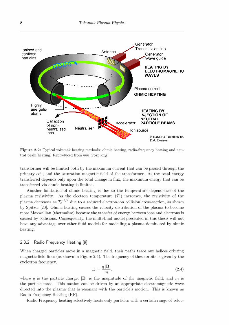
A milestone for fusion energy is the ‘burning’ plasma regime where the energy releasedby the confined fusion α particles is equal to the external heating. At this condition,the net power gain is 5 times that of the input power. To reach this condition, exter-nal heating must be used. In the to-be-built International Thermonuclear ExperimentalReactor (ITER), which is designed to have a steady-state power gain of 5, 73MW of ex-ternal heating will be used [18]. Consequently, the effects of external heating on plasmaequilibria are becoming increasingly important. As mentioned in Chapter 1, these heatingmechanisms can drive the plasma to become non-thermalised (i.e. its velocity distributionfunction becomes non-Maxwellian). Shown in Figure 2.2 are three methods of externalheating used in experimental tokamak plasmas: ohmic heating, radio-frequency heatingand neutral beam heating. Most experiments make use of all three. In this section, wediscuss these heating mechanisms and the suitability of a multi-fluid model for describingthe effect that each mechanism would have on the plasma equilibrium.
2.3.1 Ohmic Heating
Tokamak plasmas are initially formed by a toroidal electric field that ionises the atoms andaccelerates the resultant ions and electrons to form a current [19, p 238]. The bulk of thisenergy is given to the electrons, which is then transferred to the ions through electron-ionscollisions until the electrons and ions come into thermal equilibrium. This heating can alsobe considered as being caused by resistive heating (Ohmic heating), where the non-zeroresistivity, η, is caused by the electron-ion collisions. The power density released by ohmicheating is given by
PΩ = ηJ2, (2.3)
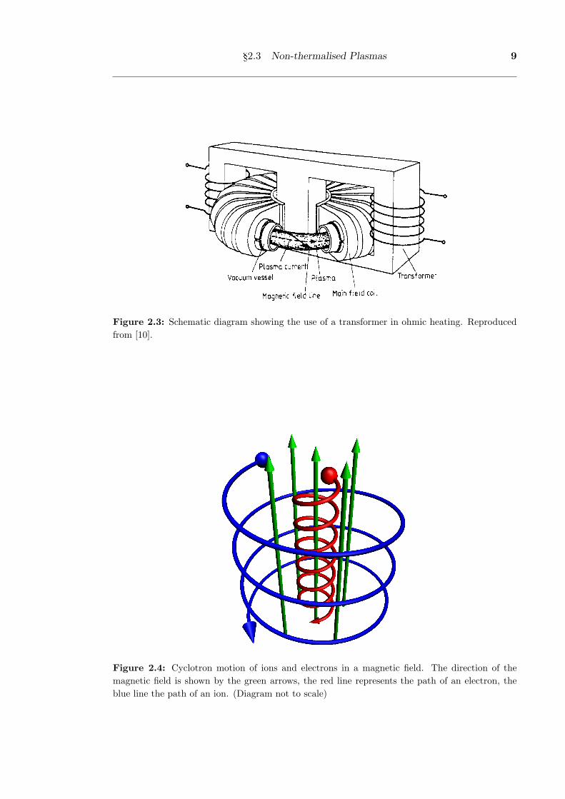
where J is the plasma current density.To create the toroidal electric field, a large transformer is used, of which the plasma
forms the secondary winding (see Figure 2.3). An increasing current in the primary wind-ings of the transformer leads to an increasing magnetic flux in the transformer, and viaFaraday’s law, a toroidal electric field in the plasma. The magnetic flux through the
8 Tokamak Plasma Physics
Figure 2.2: Typical tokamak heating methods: ohmic heating, radio-frequency heating and neu-tral beam heating. Reproduced from www.iter.org
transformer will be limited both by the maximum current that can be passed through theprimary coil, and the saturation magnetic field of the transformer. As the total energytransferred depends only upon the total change in flux, the maximum energy that can betransferred via ohmic heating is limited.
Another limitation of ohmic heating is due to the temperature dependence of theplasma resistivity. As the electron temperature (Te) increases, the resistivity of theplasma decreases as T
−3/2e due to a reduced electron-ion collision cross-section, as shown
by Spitzer [20]. Ohmic heating causes the velocity distribution of the plasma to becomemore Maxwellian (thermalise) because the transfer of energy between ions and electrons iscaused by collisions. Consequently, the multi-fluid model presented in this thesis will nothave any advantage over other fluid models for modelling a plasma dominated by ohmicheating.
2.3.2 Radio Frequency Heating [9]
When charged particles move in a magnetic field, their paths trace out helices orbitingmagnetic field lines (as shown in Figure 2.4). The frequency of these orbits is given by thecyclotron frequency,
ωc =q |B|m
, (2.4)
where q is the particle charge, |B| is the magnitude of the magnetic field, and m isthe particle mass. This motion can be driven by an appropriate electromagnetic wavedirected into the plasma that is resonant with the particle’s motion. This is known asRadio Frequency Heating (RF).
Radio Frequency heating selectively heats only particles with a certain range of veloc-
§2.3 Non-thermalised Plasmas 9
Neutral beam heating of fusion plasmas 65
I Magnetic field line Main fiieid
Stellarator windings Vncuum vessel
Figure4. Schematic illustrations of the tokamak (top), the classical I = 2 stellarator (middle)
and the modular stellarator (bottom) configurations; I is the number of pairs of stellarator
windings.
Figure 2.3: Schematic diagram showing the use of a transformer in ohmic heating. Reproducedfrom [10].
Figure 2.4: Cyclotron motion of ions and electrons in a magnetic field. The direction of themagnetic field is shown by the green arrows, the red line represents the path of an electron, theblue line the path of an ion. (Diagram not to scale)

10 Tokamak Plasma Physics
ities. This is demonstrated in the condition for an electromagnetic wave to be resonantwith the cyclotron motion [19, p 268],
v‖ =ω
k‖− l |ωc|
k‖, (2.5)
where ‖ indicates the component of a vector parallel to the magnetic field, ω is the angularfrequency of the electromagnetic wave, v is the particle’s velocity, k is the wave vector,and l = 0,±1,±2, . . . Consequently, RF heating will cause the plasma to become non-thermalised. If the heating is continuous, a dynamic equilibrium will arise in which thereis an energetic component to the velocity distribution of the plasma. The effect of thisenergetic component cannot be accurately modelled with current plasma fluid models.However, this effect can be treated by using the multi-fluid model discussed in this thesis.This can be done by approximating the energetic component of the plasma as having aMaxwellian distribution, and representing it as a second fluid.
2.3.3 Neutral Beam Heating [10]
Another method of external heating is to inject high-speed particles into the plasma. Inthis method of heating, the injected particles must be neutral, as charged particles wouldbe reflected by the plasma’s magnetic field. Once inside the plasma, the neutral particlesundergo collisional charge exchange with the ions. These ionised high-speed particles arethen confined within the plasma, and their energy will gradually be transferred to the restof the plasma through collisions. This process is known as neutral beam heating.
Neutral beam heating offers a high degree of control over where the power is distributedfrom the neutral beam, by controlling the beam energy and the position & angle of theinjected beam. Another advantage of neutral beam heating is that the location that thepower is dissipated is independent of the magnetic field, and so can be predicted moreaccurately.
The neutral beam injected into the plasma is formed by accelerating ionised particlesthrough an electric potential towards a gas vapour, where some of the ions are neutralisedby collisional charge exchange with the gas. All remaining charged particles are thendeflected out of the beam by a magnetic field before the remaining high-energy neutralparticles are injected into the plasma, as shown in Figure 2.2 on page 8. Because theneutral beam is formed by acceleration of particles through a fixed potential, the neutralbeam entering the plasma will essentially be mono-energetic, i.e. its velocity distributionwill be strongly peaked at a certain point. Once the neutral beam has entered the plasmaand become ionised, the energy of the beam is gradually transferred to the rest of theplasma through collisions.
In modern tokamak experiments, neutral beam heating is used continuously. Thiscauses a dynamic equilibrium to arise in which the energy lost by the energetic beam tothe rest of the plasma is balanced by collisional charge exchange of the injected energeticneutral particles. Hence, the plasma will have an energetic component to its velocitydistribution function, causing the distribution to be non-Maxwellian. In general, thevelocity distribution of the energetic component will not be Maxwellian, rather, it willbe a slowing-down distribution [21]. The slowing-down distribution reflects the fact thatparticles are injected into the plasma with a fixed energy, but the particles’ energiesdecrease as they undergo collisions with the rest of the plasma. Currently, the effect ofthe energetic component of the distribution function is not considered by fluid models.
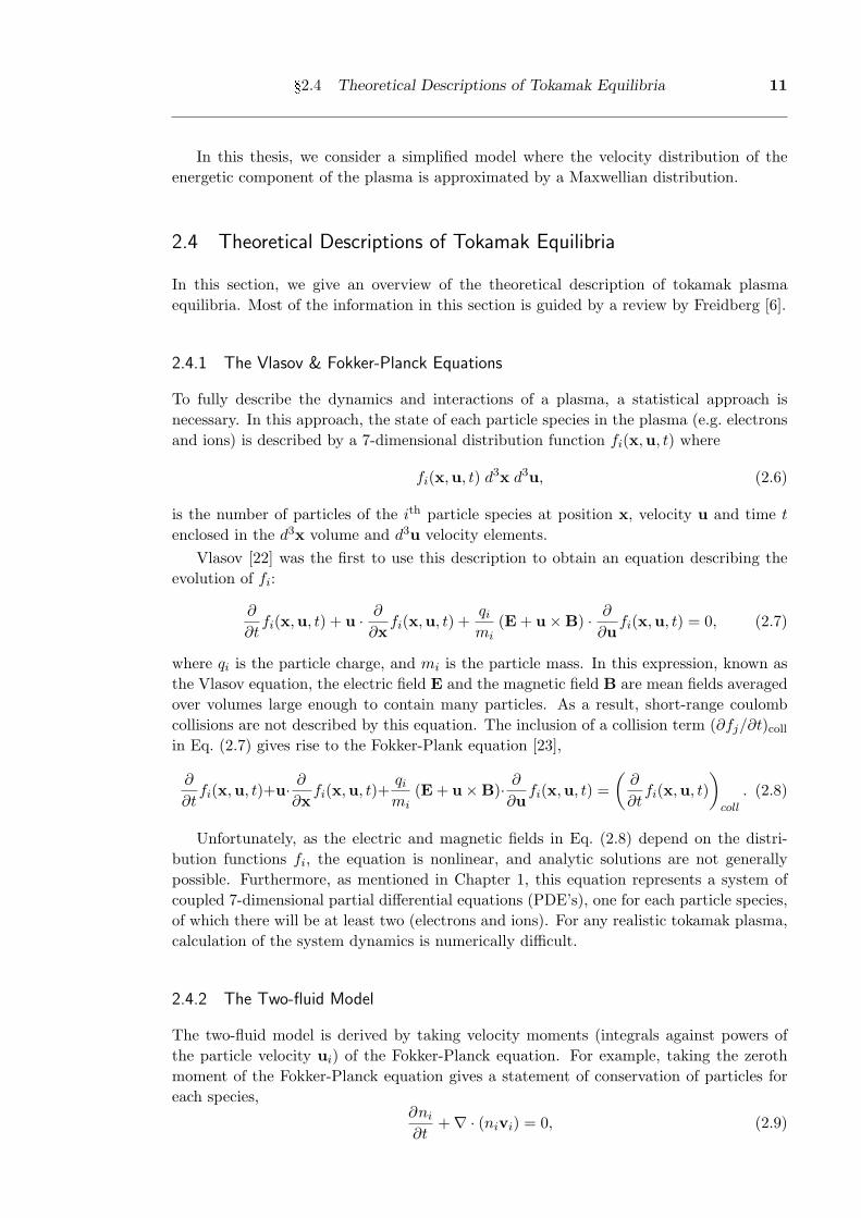
§2.4 Theoretical Descriptions of Tokamak Equilibria 11
In this thesis, we consider a simplified model where the velocity distribution of theenergetic component of the plasma is approximated by a Maxwellian distribution.
2.4 Theoretical Descriptions of Tokamak Equilibria
In this section, we give an overview of the theoretical description of tokamak plasmaequilibria. Most of the information in this section is guided by a review by Freidberg [6].
2.4.1 The Vlasov & Fokker-Planck Equations
To fully describe the dynamics and interactions of a plasma, a statistical approach isnecessary. In this approach, the state of each particle species in the plasma (e.g. electronsand ions) is described by a 7-dimensional distribution function fi(x,u, t) where
fi(x,u, t) d3x d3u, (2.6)
is the number of particles of the ith particle species at position x, velocity u and time t
enclosed in the d3x volume and d3u velocity elements.Vlasov [22] was the first to use this description to obtain an equation describing the
evolution of fi:
∂
∂tfi(x,u, t) + u · ∂
∂xfi(x,u, t) +
qi
mi(E + u×B) · ∂
∂ufi(x,u, t) = 0, (2.7)
where qi is the particle charge, and mi is the particle mass. In this expression, known asthe Vlasov equation, the electric field E and the magnetic field B are mean fields averagedover volumes large enough to contain many particles. As a result, short-range coulombcollisions are not described by this equation. The inclusion of a collision term (∂fj/∂t)collin Eq. (2.7) gives rise to the Fokker-Plank equation [23],
∂
∂tfi(x,u, t)+u· ∂
∂xfi(x,u, t)+
qi
mi(E + u×B)· ∂
∂ufi(x,u, t) =
(∂
∂tfi(x,u, t)
)coll
. (2.8)
Unfortunately, as the electric and magnetic fields in Eq. (2.8) depend on the distri-bution functions fi, the equation is nonlinear, and analytic solutions are not generallypossible. Furthermore, as mentioned in Chapter 1, this equation represents a system ofcoupled 7-dimensional partial differential equations (PDE’s), one for each particle species,of which there will be at least two (electrons and ions). For any realistic tokamak plasma,calculation of the system dynamics is numerically difficult.
2.4.2 The Two-fluid Model
The two-fluid model is derived by taking velocity moments (integrals against powers ofthe particle velocity ui) of the Fokker-Planck equation. For example, taking the zerothmoment of the Fokker-Planck equation gives a statement of conservation of particles foreach species,
∂ni
∂t+∇ · (nivi) = 0, (2.9)

12 Tokamak Plasma Physics
where ni(x, t) =∫
fi(x,u, t) d3v is the mean particle density and vi =∫
fi(x,u, t) u d3uis the mean fluid velocity. The first moment gives a statement of force balance,
mini
[∂vi
∂t+ (vi · ∇)vi
]= qini (E + vi ×B)−∇ ·
←→Pi +
∑k 6=i
Rik, (2.10)
where←→Pi is the pressure tensor for the ith particle species and Rik is the rate of momentum
transfer from the kth to the ith particle species.This process does not yield a closed system of equations because each velocity mo-
ment involves a term containing the next-higher order moment, e.g. Eq. (2.9) involves thefirst order moment (the mean fluid velocity vi), and Eq. (2.10) involves the second-ordermoment (the pressure tensor
←→Pi ). Usually only the zeroth, first and second velocity mo-
ments are taken, after which some simplifying assumptions are made to close the systemof equations. A complete derivation of the first three moments is given in Freidberg [6].
First, the scales of interest are defined. Rates of change in the plasma are assumed tobe much slower than the electron plasma frequency, ω ωpe, where ωpe =
√nee2/meε0
is the electron plasma frequency. Length scales of interest are assumed to be much largerthan the Debye length L λd where λd = |vion| /ωpe. The Debye length, λd, is a measureof the distance over which the electric field due to a single particle is ‘screened out’ by therandom motions of other particles. That is, it is the scale over which the mean fields Eand B are calculated.
Next, a second series of approximations close the system of equations. If the mean-freepath of the particles is much smaller than the dimensions of the plasma, the plasma is saidto be collision-dominated. Under this approximation, the heat flux (related to the thirdvelocity moment of the distribution function) is negligible. Also, any anisotropy in thepressure tensor will be quickly balanced, and so the pressure tensor
←→Pi can be replaced
by an isotropic scalar pressure pi.With these approximations, the two-fluid equations obtained are:
∂ρi
∂t= −∇ · (ρivi) , (2.11)
ρidvi
dt= −∇pi + niqi (E + vi ×B) +
∑k 6=i
Rik, (2.12)
d
dt
(pi
ργi
)= 0, (2.13)
where ρi = mini is the species’ mass-density, and γ is the ratio of specific heats.
2.4.3 The Ideal MHD Model
The ideal MHD model is a reduction of the two-fluid model in which the electron andion fluids are combined into a single quasi-neutral2 fluid. This is achieved by takinglinear combinations of the equations for the two-fluid model and neglecting terms of theorder me/mion. To complete the model, an expression is needed for the inter-speciesmomentum transfer, Rik. The dominant contribution to Rik between the electrons and
2Quasi-neutrality means that any charge imbalance in the fluid would be balanced on a faster timescalethan the one of interest. Consequently, qene ≈ qionnion.

§2.4 Theoretical Descriptions of Tokamak Equilibria 13
ions is electrical resistance, and it can be expressed as [24, p 43]
Rik ≈ qiniηJ, (2.14)
where η is the electrical resistivity. In the ideal MHD model, it is assumed that althoughcollisions are dominant, they are still sufficiently infrequent that the resistivity due tointer-species collisions may be neglected. If this assumption is not made, and the effectsof resistivity are retained, the model is known as the resistive MHD model.
Neglecting the resistivity of the plasma, the equations describing the ideal MHD modelare given by:
∂ρ
∂t= −∇ · ρv, (2.15)
ρdvdt
= J×B−∇p, (2.16)
d
dt
(p
ργ
)= 0, (2.17)
where ρ = ρion is the plasma mass-density, v ≈ vion is the mass-averaged velocity, p =pion+pe is the total isotropic pressure, and d/dt = ∂/∂t+(v·∇) is the convective derivative.
2.4.4 The Grad-Shafranov Equation
First derived in 1957, the Grad-Shafranov equation [25–27] is an application of the idealMHD model to describe the equilibrium of plasmas with toroidal symmetry, and zeromean fluid velocity. This regime of zero mean fluid flow was initially investigated becauseuntil the use of neutral beam heating, flows in the plasma were found to be negligiblysmall. When neutral beam heating is used, they can drive large flows in the plasma. Incertain circumstances, these large flows (in particular flow-shear) can lead to suppressionof some instabilities [28, 29]. While it is not accurate for the description of many modernexperiments, the Grad-Shafranov equation is important in that it is one of the first modelsof a plasma equilibrium in a realistic geometry.
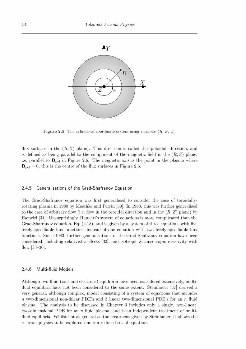
To proceed further with a discussion of the Grad-Shafranov equation, we employ acylindrical coordinate system using variables (R, Z, φ), where φ is the toroidal coordinate,as defined in Figure 2.5.
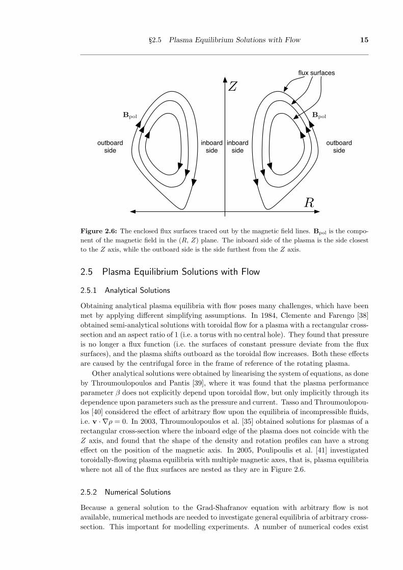
The Grad-Shafranov equation describes the plasma in terms of a set of enclosed sur-faces, called ‘flux surfaces’, traced out by the magnetic field lines. In the (R,Z) plane,the cross-section of these surfaces is traced out by the component of the magnetic field inthat plane, as shown in Figure 2.6. These flux surfaces are also the surfaces of constantpressure, and the surfaces on which the current flows. These flux surfaces are given bycontours of the parameter Ψ, where Ψ is found by solving the Grad-Shafranov equation,
R2∇ ·(∇ΨR2
)= −R2 dp(Ψ)
dΨ− f(Ψ)
df(Ψ)dΨ
, (2.18)
where p(Ψ) defines the pressure on each flux surface, and f(Ψ) = BφR defines the quantityBφR on each flux surface, with Bφ the toroidal component of the magnetic field. Bothp(Ψ) and f(Ψ) are freely specifiable functions of flux (flux functions).
Just as the gradient of Ψ defines the direction of the pressure force, it is useful tohave a definition of a direction perpendicular to ∇Ψ in the (R,Z) plane (parallel to the
14 Tokamak Plasma Physics
!
R
ZX
Y
Figure 2.5: The cylindrical coordinate system using variables (R, Z, φ).
flux surfaces in the (R,Z) plane). This direction is called the ‘poloidal’ direction, andis defined as being parallel to the component of the magnetic field in the (R,Z) plane,i.e. parallel to Bpol in Figure 2.6. The magnetic axis is the point in the plasma whereBpol = 0, this is the centre of the flux surfaces in Figure 2.6.
2.4.5 Generalisations of the Grad-Shafranov Equation
The Grad-Shafranov equation was first generalised to consider the case of toroidally-rotating plasma in 1980 by Maschke and Perrin [30]. In 1983, this was further generalisedto the case of arbitrary flow (i.e. flow in the toroidal direction and in the (R, Z) plane) byHameiri [31]. Unsurprisingly, Hameiri’s system of equations is more complicated than theGrad-Shafranov equation, Eq. (2.18), and is given by a system of three equations with fivefreely-specifiable flux functions, instead of one equation with two freely-specifiable fluxfunctions. Since 1983, further generalisations of the Grad-Shafranov equation have beenconsidered, including relativistic effects [32], and isotropic & anisotropic resistivity withflow [33–36].
2.4.6 Multi-fluid Models
Although two-fluid (ions and electrons) equilibria have been considered extensively, multi-fluid equilibria have not been considered to the same extent. Steinhauer [37] derived avery general, although complex, model consisting of a system of equations that includesn two-dimensional non-linear PDE’s and 3 linear two-dimensional PDE’s for an n fluidplasma. The analysis to be discussed in Chapter 3 includes only a single, non-linear,two-dimensional PDE for an n fluid plasma, and is an independent treatment of multi-fluid equilibria. Whilst not as general as the treatment given by Steinhauer, it allows therelevant physics to be explored under a reduced set of equations.
§2.5 Plasma Equilibrium Solutions with Flow 15
Z
R
Bpol
inboardside
outboardside
Bpol
inboardside
outboardside
flux surfaces
Figure 2.6: The enclosed flux surfaces traced out by the magnetic field lines. Bpol is the compo-nent of the magnetic field in the (R, Z) plane. The inboard side of the plasma is the side closestto the Z axis, while the outboard side is the side furthest from the Z axis.
2.5 Plasma Equilibrium Solutions with Flow
2.5.1 Analytical Solutions
Obtaining analytical plasma equilibria with flow poses many challenges, which have beenmet by applying different simplifying assumptions. In 1984, Clemente and Farengo [38]obtained semi-analytical solutions with toroidal flow for a plasma with a rectangular cross-section and an aspect ratio of 1 (i.e. a torus with no central hole). They found that pressureis no longer a flux function (i.e. the surfaces of constant pressure deviate from the fluxsurfaces), and the plasma shifts outboard as the toroidal flow increases. Both these effectsare caused by the centrifugal force in the frame of reference of the rotating plasma.
Other analytical solutions were obtained by linearising the system of equations, as doneby Throumoulopoulos and Pantis [39], where it was found that the plasma performanceparameter β does not explicitly depend upon toroidal flow, but only implicitly through itsdependence upon parameters such as the pressure and current. Tasso and Throumoulopou-los [40] considered the effect of arbitrary flow upon the equilibria of incompressible fluids,i.e. v · ∇ρ = 0. In 2003, Throumoulopoulos et al. [35] obtained solutions for plasmas of arectangular cross-section where the inboard edge of the plasma does not coincide with theZ axis, and found that the shape of the density and rotation profiles can have a strongeffect on the position of the magnetic axis. In 2005, Poulipoulis et al. [41] investigatedtoroidally-flowing plasma equilibria with multiple magnetic axes, that is, plasma equilibriawhere not all of the flux surfaces are nested as they are in Figure 2.6.
2.5.2 Numerical Solutions
Because a general solution to the Grad-Shafranov equation with arbitrary flow is notavailable, numerical methods are needed to investigate general equilibria of arbitrary cross-section. This important for modelling experiments. A number of numerical codes exist
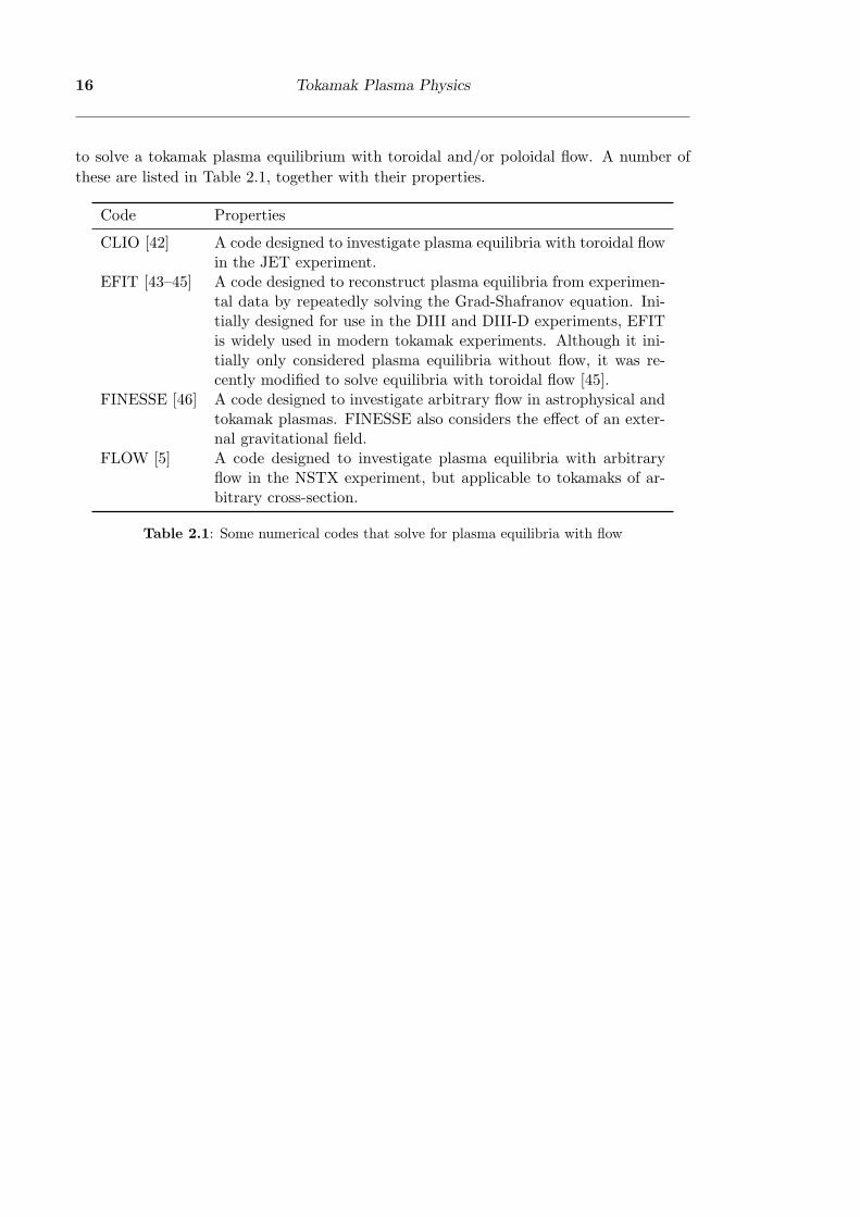
16 Tokamak Plasma Physics
to solve a tokamak plasma equilibrium with toroidal and/or poloidal flow. A number ofthese are listed in Table 2.1, together with their properties.
Code Properties
CLIO [42] A code designed to investigate plasma equilibria with toroidal flowin the JET experiment.
EFIT [43–45] A code designed to reconstruct plasma equilibria from experimen-tal data by repeatedly solving the Grad-Shafranov equation. Ini-tially designed for use in the DIII and DIII-D experiments, EFITis widely used in modern tokamak experiments. Although it ini-tially only considered plasma equilibria without flow, it was re-cently modified to solve equilibria with toroidal flow [45].
FINESSE [46] A code designed to investigate arbitrary flow in astrophysical andtokamak plasmas. FINESSE also considers the effect of an exter-nal gravitational field.
FLOW [5] A code designed to investigate plasma equilibria with arbitraryflow in the NSTX experiment, but applicable to tokamaks of ar-bitrary cross-section.
Table 2.1: Some numerical codes that solve for plasma equilibria with flow
Chapter 3
A Multi-fluid Force-balance Equation
The Grad-Shafranov equation, Eq. (2.18) on page 13, describes the equilibrium of a single-fluid plasma with zero flow under the ideal MHD approximation. In this chapter, we aimto derive an original multi-fluid plasma model that can be used to model a non-Maxwellianplasma by decomposing the electron and ion velocity distributions into multiple energy-resolved components, each approximated by a Maxwellian distribution.
To make the problem tractable, it is assumed that:
the pressure for each particle species is isotropic,
plasma resistivity is negligible,
each fluid is quasi-neutral,
the velocity distribution function for each fluid is Maxwellian, and
the plasma has toroidal symmetry.
As this work is only concerned with the plasma steady-state, all time derivatives areneglected. The derivation of the ideal MHD model by McClements and Thyagaraja [47]guided the early parts of the derivation detailed in this chapter.
3.1 Overview
A typical derivation of the ideal MHD model begins by taking velocity moments of theFokker-Planck equation, Eq. (2.8), for the electron and ion distribution functions. In themodel to be derived in this chapter, we wish to distinguish between the different energeticcomponents of the distribution functions. Consequently, we decompose the electron andion distribution functions into an arbitrary number of pairs of electron and ion distributionfunctions meeting two criteria:
1. Considered together, the electron and ion distributions of a pair are quasi-neutral.This is equivalent to the condition that the spatial profiles of the electron and iondistributions in a pair are nearly identical.
2. The velocity distributions of the electrons and ions of a pair are similar, but suf-ficiently separate from the velocity distributions of the other pairs. Because theenergy transferred by Coulomb collisions (Rutherford scattering) is proportional tothe inverse square of the difference in velocities of two particles undergoing a collision[19, p 54], the energy transferred between particles in the same pair will dominatethe transfer of energy between particles in different pairs.
17
18 A Multi-fluid Force-balance Equation
We index the different components of the electron and ion distribution functions collec-tively by the subscript i, while the pairs are indexed by the subscript j. For example,if the electron and ion velocity distributions are decomposed into n pairs, i will satisfy1 ≤ i ≤ 2n, and j, 1 ≤ j ≤ n. Initially, each component will be considered separately,before combining the pairs to give n quasi-neutral fluids.
The starting equations for this derivation are the zeroth and first order moments of theFokker-Planck equation (Eq. (2.9) and Eq. (2.10)), Maxwell’s equations, and an equationof state with a form to be specified later in the derivation. By specifying the equation ofstate as late in the derivation as possible, earlier results are independent of the equationof state eventually chosen.
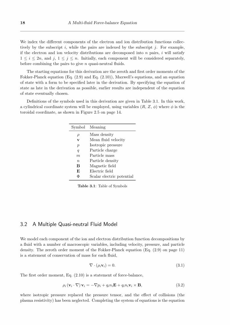
Definitions of the symbols used in this derivation are given in Table 3.1. In this work,a cylindrical coordinate system will be employed, using variables (R, Z, φ) where φ is thetoroidal coordinate, as shown in Figure 2.5 on page 14.
Symbol Meaning
ρ Mass densityv Mean fluid velocityp Isotropic pressureq Particle chargem Particle massn Particle densityB Magnetic fieldE Electric fieldΦ Scalar electric potential
Table 3.1: Table of Symbols
3.2 A Multiple Quasi-neutral Fluid Model
We model each component of the ion and electron distribution function decompositions bya fluid with a number of macroscopic variables, including velocity, pressure, and particledensity. The zeroth order moment of the Fokker-Planck equation (Eq. (2.9) on page 11)is a statement of conservation of mass for each fluid,
∇ · (ρivi) = 0. (3.1)
The first order moment, Eq. (2.10) is a statement of force-balance,
ρi (vi · ∇)vi = −∇pi + qiniE + qinivi ×B, (3.2)
where isotropic pressure replaced the pressure tensor, and the effect of collisions (theplasma resistivity) has been neglected. Completing the system of equations is the equation
§3.2 A Multiple Quasi-neutral Fluid Model 19
of state, which will be specified later, and Maxwell’s equations:
∇ ·E =∑
i
qini, (3.3)
∇ ·B = 0, (3.4)
∇×E = 0, (3.5)
∇×B = µ0J. (3.6)
Solving this set of equations numerically is in general a non-trivial exercise due to thelarge number of interdependent variables and complicated geometry. In order to solve thissystem of equations numerically, it will be necessary to spend some time simplifying thesystem by reducing the number of variables and simplifying the geometry. The first stepwill be to group the ion and electron fluids into their quasi-neutral pairs, and approxi-mate each pair as an ideal fluid (i.e. negligible resistivity). Next, vector components ofthe force-balance equations are taken to obtain a number of freely-specifiable flux func-tions representing certain properties of the plasma equilibrium, and a second order partialdifferential equation.
Consider now, the force balance equation for the electron component of one of thesequasi-neutral fluids,
0 = −∇pj,e + qj,enj,eE + qj,enj,evj,e ×B, (3.7)
where the left hand side of Eq. (3.2) is neglected due to the comparatively small mass ofthe electron. In plasmas for which the electrons are well-confined by the electromagneticfields, the pressure of the electron species may also be neglected, yielding
E + vj,e ×B = 0, (3.8)
for the electron component in each quasi-neutral fluid.
To model the plasma as a collection of interacting ideal MHD fluids, it is necessary towrite all quantities in terms of the parameters of the quasi-neutral ideal MHD fluid, e.g.the fluid velocity vj and the fluid current Jj . The fluid velocity is defined as
vj =mj,ionnj,ionvj,ion + mj,enj,evj,e
mj,ionnj,ion + mj,enj,e≈ vj,ion, (3.9)
where the fluid velocity is essentially the velocity of the ion component, due to the smallmass of the electron. The current of the fluid is defined as
Jj = nj,ionqj,ionvj,ion + nj,eqj,evj,e. (3.10)
As the ion and electron components in each fluid form a quasi-neutral pair, there is alsoa quasi-neutrality condition on the fluid that can be written as
nj,eqj,e + nj,ionqj,ion = 0. (3.11)
Using these three expressions, the electron component’s velocity is eliminated fromEq. (3.8) to give
E− 1nj,ionqj,ion
Jj ×B + vj ×B = 0. (3.12)
20 A Multi-fluid Force-balance Equation
If the electron and ion components have roughly the same velocity in the direction per-pendicular to the magnetic field, then the Hall term in the above equation (the secondterm) can be neglected compared to the vj ×B term. Explicitly, the assumption made is
|Jj ×B|nj,ionqj,ion
= |(vj,ion − vj,e)×B| |vj ×B| , (3.13)
for each fluid in the plasma. By doing this, the usual ideal MHD equation is arrived atfor each fluid,
E + vj ×B = 0. (3.14)
This is an important equation, and a number of results will be obtained from it. Atpresent, it is enough to note that it is one of two equations that will be obtained fromthe force-balance equation (Eq. (3.2) on page 18) for the electron and ion components ineach quasi-neutral fluid. The second equation is obtained by summing the force-balanceequation (Eq. (3.7)) over the electron and ion species in a fluid,
ρj (vj · ∇)vj = −∇pj + Jj ×B, (3.15)
where ρj is the mass-density of the fluid and pj is the isotropic partial pressure exerted bythe fluid. Note that the electric field term has disappeared due the the quasi-neutrality ofeach fluid.
3.3 Flux Functions for Velocity
At this point, the force-balance equations for each particle species have been transformedinto two equations, an equation describing the fluid as a perfect conductor, Eq. (3.14), anda force-balance equation, Eq. (3.15). The aim in this section is to obtain from Eq. (3.14),a number of flux functions describing the velocity distribution of the plasma. Before doingthis, the constraints given in Eq. (3.1), Eq. (3.4), and Eq. (3.5) must be considered.
As the electric field is curl-free (from Eq. (3.5) on the previous page), it can be writtenas the gradient of a scalar field,
E = −∇Φ(R,Z), (3.16)
where, due to toroidal symmetry, Φ does not depend on the toroidal co-ordinate. Also, asboth the magnetic field, B, and the fluid mass flux, ρjvj , are divergence-free, they can bewritten in the following form:
B =1R∇Ψ× eφ + Bφeφ, (3.17)
ρjvj =1R∇ζj × eφ + ρjvj,φeφ, (3.18)
where Ψ is the poloidal magnetic flux, Bφ is the toroidal magnetic field, ζj is the poloidalmass flux for the jth fluid, vj,φ is the toroidal component of the jth fluid velocity, and eφ
is a unit vector in the φ direction.As the toroidal component of Eq. (3.16) is zero, the toroidal component of the second
term of the ideal MHD equation must also be zero,
(vj ×B)φ = 0. (3.19)

§3.4 The Fluid Force-balance Equation 21
This can be simplified using the expansions for ρjvj and B in Eq. (3.18) and Eq. (3.17)respectively. After some algebra, the cross product of these two equations is expressed as
ρjvj ×B =1
R2∇ζj ×∇Ψ−
Bφ
R∇ζj +
ρjvj,φ
R∇Ψ. (3.20)
Because ζj and Ψ do not depend on the toroidal co-ordinate, Eq. (3.19) gives
∇ζj ×∇Ψ = 0, (3.21)
=⇒ ζj = ζj(Ψ). (3.22)
The latter equation can also be written as Ψ = Ψ(ζj), however it is more convenient tohave all the ζj variables written in terms of the single variable Ψ. ζj(Ψ) is called a fluxfunction because it is a function of the poloidal magnetic flux, Ψ, as defined in §2.4.4. Tosimplify solving the plasma equilibrium, we aim to write as much of the plasma equilibriumas possible in terms of Ψ, and obtain an equation describing the solution for Ψ.
Another flux function can be extracted from the ideal MHD approximation by takingthe curl of each term in the ideal MHD equation, Eq. (3.14), and applying Faraday’s law(Eq. (3.5) on page 19). This gives the following result,
∇× (vj ×B) = 0. (3.23)
Substituting Eq. (3.20) into Eq. (3.23), a second flux function, Ωj(Ψ), is obtained fromthe ideal MHD equation,
Ωj(Ψ) =vj,φ
R−
Bφ
ρjRζ ′j , (3.24)
where a prime denotes a derivative with respect to the poloidal flux, Ψ. This equation isa poloidal-flow-modified equation for the toroidal angular frequency of the flux surfaces.In a plasma with purely toroidal flow, ζ ′j would be zero and the flux surfaces would rotaterigidly in the toroidal direction because ωj = vj,φ/R would be a flux function. However,with poloidal flow, ζ ′j is non-zero, and this is no longer the case.
3.4 The Fluid Force-balance Equation
The previous section reduced the ideal MHD equation to two freely-specifiable flux func-tions, ζj(Ψ) and Ωj(Ψ). In this section and the next, the aim is to simplify the fluidforce-balance equation (Eq. (3.15) on the preceding page). In particular, we aim to pa-rameterise the plasma equilibrium in terms of the poloidal magnetic flux, Ψ, and obtain anequation describing the solution to Ψ. Accordingly, in this section, the fluid force-balanceequation is expanded in terms of Ψ. This is done in anticipation of Section 3.5 where itsvector components are taken.
In order to reduce the number of different variables in the force balance equation, it isuseful to decompose the magnetic field into the components due to the currents Jj , andthe component due to the externally applied field. Ampere’s law can then be applied toeach component of the total magnetic field to write the current Jj in terms of the magneticfield Bj that it produces. In this way, the Jj×B term in Eq. (3.15) can be written entirelyin terms of magnetic fields.
We decompose the total magnetic field in terms of the components due to each current,

22 A Multi-fluid Force-balance Equation
and an externally-produced field,
B =∑
j
Bj + Bext, (3.25)
where Bj is the magnetic field produced by Jj , and Bext is the externally applied magneticfield. This decomposition is valid, because each of the currents Jj are physical currents.Thus, by the superposition principle, the total magnetic field will be the sum of thecomponents due to each fluid current Jj in the plasma and the component Bext due tocurrents external to the plasma.
Because these magnetic field components represent physical magnetic fields, their di-vergences must be zero:
∇ ·Bj = 0, (3.26)
∇ ·Bext = 0. (3.27)
Consequently, Bj and Bext can be expanded in a similar way to the total magnetic fieldin Eq. (3.17):
Bj =1R∇Ψj × eφ + Bj,φeφ, (3.28)
Bext =1R∇Ψext × eφ + Bext,φeφ. (3.29)
Ampere’s law can now be applied to Bj and Bext to obtain expressions for Jj and Jext interms of the magnetic fields they produce,
∇×Bj = −R∇ ·(
1R2∇Ψj
)eφ +
1R∇ (Bj,φR)× eφ = µ0Jj , (3.30)
∇×Bext = −R∇ ·(
1R2∇Ψext
)eφ +
1R∇ (Bext,φR)× eφ = µ0Jext. (3.31)
As Bext is, by definition, caused by currents outside of the plasma, Jext = 0 must hold inthe plasma. As the poloidal and toroidal terms in Eq. (3.31) are orthogonal, applying thiscondition gives
∇ ·(
1R2∇Ψext
)= 0, (3.32)
Bext,φR = constant. (3.33)
Using Eq. (3.30) for Jj , and Eq. (3.17) for B, the Jj × B term in the force-balanceequation (Eq. (3.15)) can be rewritten as
Jj ×B = − 1µ0∇ ·(
1R2∇Ψj
)∇Ψ− 1
µ0
Bφ
R∇ (Bj,φR)− 1
µ0
1R2
[∇Ψ×∇ (Bj,φR)] . (3.34)
Now that the Jj×B term in the force-balance equation has been expanded in terms ofthe poloidal magnetic fluxes Ψ and Ψj , we turn our attention to the term on the left handside of the force-balance equation, Eq. (3.15). To expand this in terms of Ψ, the expansionfor ρjvj in Eq. (3.18) will be used. As it has already been shown that the poloidal massflux ζj is a function of Ψ in Eq. (3.22), this expansion will then enable the left hand side

§3.5 Flux Functions from the Force-balance Equation 23
of the force-balance equation to be written in terms of Ψ as well.First, a vector identity is used to expand the convective derivative:
ρj (vj · ∇)vj = ρj (∇× vj)× vj +ρj
2∇v2
j . (3.35)
Substituting the expansion for ρjvj in Eq. (3.18) into this equation and simplifying, allowsus to rewrite this as
ρj (vj · ∇)vj = −∇ ·(∇ζj
ρjR2
)∇ζj +
1R2
[∇ (vj,φR)×∇ζj ]−ρj
2R2∇(v2j,φR2
)+
ρj
2∇v2
j .
(3.36)Because ζj is a function of Ψ, the gradient terms in this expression can be written in termsof Ψ using ∇ζj = ζ ′j∇Ψ. Substituting this into the expansion above gives
ρj (vj · ∇)vj = −∇ ·(
1ρR2
ζ ′j∇Ψ)
+1
R2ζ ′j [∇ (vj,φR)×∇Ψ]− ρj
2R2∇(v2j,φR2
)+
ρj
2∇v2
j .
(3.37)Combining the expansions for the convective derivative term and for Jj×B allows the
force-balance equation to be written as
−∇ ·(
1ρjR2
ζ ′j∇Ψ)
ζ ′j∇Ψ +1
R2ζ ′j [∇ (vj,φR)×∇Ψ]− ρj
2R2∇(v2j,φR2
)+
ρj
2∇v2
j
= −∇pj −1µ0∇ ·(
1R2∇Ψj
)∇Ψ− 1
µ0
Bφ
R∇ (Bj,φR) +
1µ0
1R2
[∇ (Bj,φR)×∇Ψ] .
(3.38)
Although this equation is significantly more complicated than Eq. (3.15), it makes theprocess of taking components in the ∇Ψ and ∇Ψ× eφ directions in the next section muchsimpler. Additionally, as much of the plasma equilibrium as possible has been written interms of the single parameter Ψ.
3.5 Flux Functions from the Force-balance Equation
In this section, vector components of Eq. (3.38) are taken to obtain two more flux functions.To begin with, we consider the toroidal component of Eq. (3.38),
1R2
ζ ′j [∇ (vj,φR)×∇Ψ] =1µ0
1R2
[∇ (Bj,φR)×∇Ψ] . (3.39)
Rearranging this gives another flux function,
fj(Ψ) = Bj,φR− µ0vj,φRζ ′j . (3.40)
In a plasma with no poloidal flow, ζ ′j would be zero and Eq. (3.40) reduces to the expressionf(Ψ) = BφR for the Grad-Shafranov equation, discussed in §2.4.4.
This new flux function, Eq. (3.40), can be used together with the definition of Ωj
in Eq. (3.24) on page 21 to obtain an expression for the toroidal component of the totalmagnetic field. This is useful, because the expanded force-balance equation, Eq. (3.38)involves Bφ, and it would be preferable to have as much of the force-balance equation aspossible written in terms of the poloidal flux Ψ. Simultaneously solving Eq. (3.40) with

24 A Multi-fluid Force-balance Equation
the definition of Ωj in Eq. (3.24) to eliminate vj,φ gives
BφR =
∑j fj(Ψ) + Bext,φR + µ0
∑j R2ζ ′jΩj
1− µ0∑
j1ρj
ζ ′2j, (3.41)
where a prime indicates a derivative with respect to Ψ. This equation can be simplifiedby defining
f(Ψ) =∑
j
fj(Ψ) + Bext,φR, (3.42)
where Bext,φR is a constant, from Eq. (3.33) on page 22. Substituting this into Eq. (3.41)gives
BφR =f(Ψ) + µ0
∑j R2ζ ′j(Ψ)Ωj(Ψ)
1− µ0∑
j1ρj
ζ ′2j (Ψ). (3.43)
So far, only one flux function has been obtained from the force-balance equation,fj(Ψ) in Eq. (3.40). Another flux function can be obtained from the poloidal componentof the expanded force-balance equation (Eq. (3.38) on the preceding page). Subtractingthe toroidal component, which has already been considered, the force-balance equationbecomes
−∇ ·(
1ρjR2
ζ ′j∇Ψ)
ζ ′j∇Ψ− ρj
2R2∇(v2j,φR2
)+
ρj
2∇v2
j
= −∇pj −1µ0∇ ·(
1R2∇Ψj
)∇Ψ− 1
µ0
Bφ
R∇ (Bj,φR) .
(3.44)
To obtain the poloidal component of this equation, its scalar product is taken with a unitvector in the poloidal direction (see Figure 2.6 on page 15 for a definition of the poloidaldirection),
bpol =Bpol
|Bpol|=∇Ψ× eφ
|∇Ψ|, (3.45)
where the subscript ‘pol’ refers to the poloidal component. Noting that bpol · ∇Ψ = 0,taking the scalar product of bpol with Eq. (3.44) gives
− ρj
2R2bpol · ∇
(v2j,φR2
)+
ρj
2bpol · ∇v2
j = −bpol · ∇pj −1µ0
Bφ
Rbpol · ∇ (Bj,φR) . (3.46)
As (bpol ·∇)Ψ = 0, bpol points along surfaces of constant poloidal flux, Ψ. Hence, definingl as the length along surfaces of constant poloidal flux, we obtain
bpol · ∇ =∂
∂l. (3.47)
Applying this to Eq. (3.46) yields
− ρj
2R2
∂
∂l
(v2j,φR2
)+
ρj
2∂
∂lv2
j +∂
∂lpj +
1µ0
Bφ
R
∂
∂l(Bj,φR) = 0. (3.48)
We seek to recast Eq. (3.48) in the form ∂∂l (· · · ) = 0, and so generate a poloidal flux
§3.5 Flux Functions from the Force-balance Equation 25
function. The first term in Eq. (3.48) can be simplified to
− ρj
2R2
∂
∂l
(v2j,φR2
)= −
ρjvj,φ
R
∂
∂l(vj,φR) . (3.49)
Making use of the definition of fj(Ψ) in Eq. (3.40) on page 23 to expand the last term inEq. (3.48) gives
1µ0
Bφ
R
∂
∂l(Bj,φR) =
Bφ
Rζ ′j
∂
∂l(vj,φR) , (3.50)
where the identities ∂∂l fj(Ψ) = 0 and ∂
∂l (ζ′j(Ψ)) = 0 have been applied. Adding Eq. (3.49)
and Eq. (3.50) gives, after some minor manipulation,
− ρj
2R2
∂
∂l
(v2j,φR2
)+
1µ0
Bφ
R
∂
∂l(Bj,φR) = −ρj
∂
∂l(Ωj(Ψ)vj,φR) . (3.51)
Further progress requires an equation of state to be specified in order to write the thirdterm of Eq. (3.48) in the form ρj
∂∂l (· · · ). In this work, it is assumed that the plasma is
highly collisional, specifically that it has a high rate of intra-fluid collisions. As a result, thevelocity distribution at each point in the plasma will be locally-Maxwellian. This meansthat at each point in the plasma, a temperature can be well-defined. The importance ofthis assumption was discussed in more detail in §2.3.
As a consequence of this assumption, each fluid is described by the ideal MHD adiabaticequation. In steady-state, this is
vj · ∇
(pj
ργj
j
)= 0, (3.52)
where γj is the ratio of specific heats. This equation is a statement of conservation ofentropy in the fluid’s frame.
Applying the expansion of ρjvj in Eq. (3.18) on page 20 to Eq. (3.52), another fluxfunction is obtained,
σj(ζj) =pj
ργj
j
. (3.53)
Noting that ζj is a function of Ψ, the above equation is more usefully written as
σj(Ψ) =pj
ργj
j
. (3.54)
This equation can be used to write the third term in Eq. (3.48) in the form ρj∂∂l (· · · ),
∂
∂lpj = ρj
∂
∂l
(γj
γj − 1σj(Ψ)ργj−1
j
). (3.55)
Substituting Eq. (3.51) and Eq. (3.55) into Eq. (3.48) yields an equation that can bewritten in the desired form ∂
∂l (· · · ) = 0,
ρj∂
∂l
(12v2
j +γj
γj − 1σj(Ψ)ργj−1
j − Ωj(Ψ)vj,φR
)= 0. (3.56)
Remembering that l is defined as the length along surfaces of constant Ψ, the function
26 A Multi-fluid Force-balance Equation
inside the parentheses in this equation must be purely a function of the poloidal flux Ψ,
Hj(Ψ) =12v2
j +γj
γj − 1σj(Ψ)ργj−1
j − Ωj(Ψ)vj,φR. (3.57)
This is a generalised Bernoulli equation for each fluid in the plasma. It describes therelationship between vj , pressure and rotational potential energy Ωjvj,φR on each fluxsurface in the plasma.
3.6 The Generalised Grad-Shafranov Equation
Two flux functions have now been derived from the fluid force-balance equation (Eq. (3.15)on page 20). A generalised toroidal flux function fj(Ψ) in Eq. (3.40), was obtained bytaking the toroidal component of the force-balance equation. The Bernoulli equation,Hj(Ψ) in Eq. (3.57) was derived by taking the component of the force-balance equationparallel to the magnetic field in the poloidal direction, i.e. along surfaces of constant Ψ.
A third equation can be derived from the force-balance equation, and that is themulti-fluid flow-modified generalisation of the Grad-Shafranov equation. This equation isobtained by taking the remaining component of the force-balance equation, that is, thecomponent parallel to ∇Ψ.
Making use of the product rule,
∇ · (fA) = f (∇ ·A) + A · (∇f) , (3.58)
the following identity is obtained
∇ ·(
1ρj
ζ ′2j1
R2∇Ψ
)= ζ ′j∇ ·
(ζ ′jρj
1R2∇Ψ
)+
ζ ′jζ′′j
ρjR2|∇Ψ|2 . (3.59)
Substituting this equation into the poloidal component of the force-balance equa-tion, Eq. (3.44) on page 24, gives
∇ ·[
1R2
(1µ0∇Ψj −
1ρj
ζ ′2j ∇Ψ)]∇Ψ +
ζ ′jζ′′j
ρjR2|∇Ψ|2∇Ψ
− ρj
2R2∇(v2j,φR2
)+
ρj
2∇v2
j +∇pj +1µ0
Bφ
R∇ (Bj,φR) = 0.
(3.60)
The aim now is to make use of all the flux functions obtained so far to reduce Eq. (3.60)to one partial differential equation in two spatial dimensions. Making use of the Bernoulliequation, Eq. (3.57), the fourth term in Eq. (3.60) can be written as
ρj∇12v2
j =ρjH′j∇Ψ + ρjΩ′
jvj,φR∇Ψ + ρjΩj∇ (vj,φR)
− γj
γj − 1ρ
γj
j σ′j∇Ψ− γjργj−1j σj∇ρj .
(3.61)
Using the equation of state, Eq. (3.54) on the previous page, the fifth term in Eq. (3.60)gives
∇pj = σ′jργj
j ∇Ψ + σjγjργj−1j ∇ρj . (3.62)
Substituting the definition of fj(Ψ), Eq. (3.40) on page 23, into the last term in Eq. (3.60)
§3.6 The Generalised Grad-Shafranov Equation 27
yields1µ0
Bφ
R∇ (Bj,φR) =
Bφ
R
[1µ0
f ′j∇Ψ + ζ ′j∇ (vj,φR) + vj,φRζ ′′j∇Ψ]
. (3.63)
Substituting Eq. (3.61), Eq. (3.62), Eq. (3.63), and the definition of Ωj in Eq. (3.24) onpage 21 into Eq. (3.60) yields after some algebra,
1µ0∇ ·[
1R2
(∇Ψj − µ0
1ρj
ζ ′2j ∇Ψ)]
=− ρjH′j − ρjR
2ΩjΩ′j −BφR
(1µ0
f ′jR2
+ Ω′jζ
′′j
)+
ργj
j
γj − 1σ′j −
1R2
ζ ′jζ′′j
ρj
[|∇Ψ|2 + (BφR)2
],
(3.64)
where BφR is given as a function of (Ψ, ρj, R) in Eq. (3.43) on page 24.
This equation is a per-fluid flow-modified Grad-Shafranov equation describing the equi-librium of a multi-fluid plasma in terms of the fluid mass-density, ρj , and the fluid’s poloidalmagnetic flux, Ψj . For an n-fluid plasma, Eq. (3.64) is a set of n coupled two-dimensionalsecond-order partial differential equations for the poloidal magnetic flux, Ψj , in terms ofthe fluid densities, ρj , and the five flux functions ζj(Ψ), Hj(Ψ), Ωj(Ψ), fj(Ψ) and σj(Ψ).Eq. (3.64) is not a closed system and will need to be solved simultaneously with the n
Bernoulli equations which can be written in the following convenient form:
Hj(Ψ) =12
(ζ ′j
ρjR
)2 [|∇Ψ|2 + (BφR)2
]+
γj
γj − 1σjρ
γj−1j − 1
2(RΩj)
2 , (3.65)
where again, BφR is given in Eq. (3.43). These n algebraic equations can be solvedsimultaneously with the n Grad-Shafranov PDE’s to complete the system.
If we limit ourselves to only considering the total poloidal flux, and not the flux dueto each fluid (i.e. if we’re only interested in the total toroidal current, and not the detailsof the contributions from each fluid), the system can be reduced further. To achieve this,Eq. (3.64) is summed over the n fluids,
1µ0∇ ·
1− µ0
∑j
1ρj
ζ ′2j
∇ΨR2
=−∑
j
ρjH′j −R2
∑j
ρjΩjΩ′j
−BφR
1µ0
f ′
R2+∑
j
Ω′jζ
′′j
+∑
j
ργj
j
γj − 1σ′j −
∑j
1R2
ζ ′jζ′′j
ρj
[|∇Ψ|2 + (BφR)2
],
(3.66)
where Eq. (3.32) and Eq. (3.42) have been used to simplify some terms. This system ofequations is much simpler to solve than Eq. (3.64); instead of solving for the n variablesΨj with n non-linear partial differential equations, only the total poloidal flux, Ψ, needsto be solved for with only a single non-linear partial differential equation. This system hasa significantly reduced computational complexity compared to the system of equations atthe start of this chapter.
28 A Multi-fluid Force-balance Equation
3.7 Reductions to Previous Results
In this section, we compare our Bernoulli equation, Eq. (3.65), and modified Grad-Shafranov equation, Eq. (3.66) to previous results.
3.7.1 Reduction to Guazzotto et al. [5]
The paper by Guazzotto et al. describes a single-fluid plasma equilibrium solver, FLOW.Their solver works by an iterative process whereby it swaps back and forth between solvingthe Bernoulli equation and the Grad-Shafranov equation. This is known as current-fielditeration.
Their Bernoulli equation can be obtained by combining Eq. (16) and Eq. (17) in [5].Written in the notation of this work1, their Bernoulli equation is
H(Ψ) =12
(ζ ′(Ψ)
ρ|B|)2
+γ
γ − 1σ(Ψ)ργ−1 − 1
2(RΩ(Ψ))2 . (3.67)
Using the definition of Ψ in Eq. (3.17) on page 20 to replace the[|∇Ψ|2 + (BφR)2
]term
in Eq. (3.65) yields
Hj(Ψ) =12
(ζ ′j(Ψ)
ρj|B|)2
+γj
γj − 1σj(Ψ)ργj−1
j − 12
(RΩj(Ψ))2 . (3.68)
Clearly in the single-fluid limit where the j subscripts are dropped, Eq. (3.68) andEq. (3.67) are equivalent.
In Guazzotto et al. [5], the Grad-Shafranov equation (Eq. (19a) of [5]) reads (whenwritten in the notation of this work, using the transformation in footnote 1)
1µ0∇ ·[(
1− µ0ζ ′2
ρ
)∇ΨR2
]=− ρH ′ − ρvφRΩ′ +
ργ
γ − 1σ′
− 1µ0
Bφ
Rf ′ −B · vζ ′′.
(3.69)
The multi-fluid Grad-Shafranov equation derived in Eq. (3.66) on the preceding page canbe written in a similar form,
1µ0∇ ·
1− µ0
∑j
1ρj
ζ ′2j
∇ΨR2
=−∑
j
ρjH′j −
∑j
ρjvj,φRΩ′j +
∑j
ργj
j
γj − 1σ′j
− 1µ0
Bφ
Rf ′ −B ·
∑j
vjζ′′j .
(3.70)
Once more, in the single-fluid limit where the j subscripts are dropped and the sumsdisappear, Eq. (3.70) reduces to Eq. (3.69).
1The transformation used is: Φ(Ψ) 7→ √µ0ζ
′(Ψ), S(Ψ) 7→ σ(Ψ), F (Ψ) 7→ f(Ψ). Note that Eq. (15) in[5] has an incorrect sign in the numerator, and Eq. (19a) in [5] is missing a factor of 1
µ0on the LHS, and
in the first term of the RHS.
§3.7 Reductions to Previous Results 29
3.7.2 Reduction to McClements and Thyagaraja [47]
The working of McClements and Thyagaraja helped guide this analysis, so it is not unsur-prising that there are similarities between the method used here and that in McClementsand Thyagaraja [47]. However, there are some superficial differences due to a differentchoice of units and differing notations for some flux functions.
In McClements and Thyagaraja [47], the the effects due to gravitation (from the plasmaitself, and external sources) are included, an effect ignored in this thesis. This differenceis only apparent in their Bernoulli equation, (Eq. (31) of [47]). Written in the notation ofthis thesis2, their Bernoulli equation is
H(Ψ) =12v2 + V +
γ
γ − 1σ(Ψ)ργ−1 − Ω(Ψ)Rvφ, (3.71)
where V is the gravitational potential. The equivalent equation in this work is Eq. (3.57)on page 26,
Hj(Ψ) =12v2
j +γj
γj − 1σj(Ψ)ργj−1
j − Ωj(Ψ)vj,φR. (3.72)
This equation reduces identically to Eq. (3.71) in the single-fluid negligible-gravity limitwhere the j subscripts are dropped, and the gravitational potential in Eq. (3.71) is ne-glected.
The modified Grad-Shafranov equation obtained by McClements and Thyagaraja(Eq. (33) in [47]) written in the notation of this thesis (using the transformation in foot-note 2) is
1µ0
∂
∂Z
[(1− µ0
ζ ′2
ρ
)∂Ψ∂Z
]+
1µ0
R∂
∂R
[(1− µ0
ζ ′2
ρ
)1R
∂Ψ∂R
]+
ζ ′ζ ′′
ρ
[(∂Ψ∂R
)2
+(
∂Ψ∂Z
)2]
+ ρR2H ′ + ρR2Ω′Rvφ
−R2σ′
γ − 1ργ +
1µ0
BφRf ′ + (BφR) (vφR) ζ ′′ = 0.
(3.73)
This equation can be rewritten using the divergence and gradient operators as
1µ0
R2∇ ·[(
1− µ0ζ ′2
ρ
)∇ΨR2
]=− ζ ′ζ ′′
|∇Ψ|2
ρ− ρR2H ′ − ρR2Ω′Rvφ
+R2σ′
γ − 1ργ − 1
µ0BφRf ′ − (BφR) (vφR) ζ ′′.
(3.74)
The Grad-Shafranov equation obtained in Eq. (3.70) on the facing page can be written in
2The transformation used is F (Ψ) 7→ ζ(Ψ), Λ(Ψ) 7→ − 14π
f(Ψ). Additionally, CGS units are transformedinto SI units.

30 A Multi-fluid Force-balance Equation
a similar form to Eq. (3.74) by multiplying by R2 and expanding the B · vj term,
1µ0
R2∇ ·
1− µ0
∑j
1ρj
ζ ′2j
∇ΨR2
=− |∇Ψ|2∑
j
1ρj
ζ ′jζ′′j −
∑j
ρjR2H ′
j
−∑
j
ρjvj,φRΩ′jR
2 +∑
j
R2ρ
γj
j
γj − 1σ′j
− 1µ0
BφRf ′ −BφR∑
j
vj,φRζ ′′j .
(3.75)
Dropping all the j subscripts and sums in Eq. (3.75), this equation reduces exactly toEq. (3.74).
3.8 Summary of the Derivation
In this chapter, a set of equations have been derived to model the behaviour of a plasma.In particular, the model has been developed with the aim of modelling plasmas for whicha temperature cannot be defined at each point in the plasma. The solution to this problemhas been to decompose the plasma into multiple fluids, each with a well-defined temper-ature at each point in the plasma. This solution is represented by one non-linear partialdifferential equation, two algebraic equations and several freely-specifiable flux functions.The equations are: the equation for the toroidal component of the magnetic field, Eq. (3.43)on page 24,
BφR =f(Ψ) + µ0
∑j R2ζ ′j(Ψ)Ωj(Ψ)
1− µ0∑
j1ρj
ζ ′2j (Ψ), (3.76)
the Bernoulli equation for each fluid, Eq. (3.68) on page 28,
Hj(Ψ) =12
(ζ ′j
ρjR
)2 [|∇Ψ|2 + (BφR)2
]+
γj
γj − 1σjρ
γj−1j − 1
2(RΩj)
2 , (3.77)
and the modified Grad-Shafranov equation, Eq. (3.66) on page 27,
1µ0∇ ·
1− µ0
∑j
1ρj
ζ ′2j
∇ΨR2
=−∑
j
ρjH′j −R2
∑j
ρjΩjΩ′j
−BφR
1µ0
f ′
R2+∑
j
Ω′jζ
′′j
+∑
j
ργj
j
γj − 1σ′j −
∑j
1R2
ζ ′jζ′′j
ρj
[|∇Ψ|2 + (BφR)2
].
(3.78)
The flux functions that need to be specified are: ζj(Ψ) defined in Eq. (3.22) on page 21,Ωj(Ψ) defined in Eq. (3.24) on page 21, f(Ψ) defined in Eq. (3.42) on page 24 and Hj(Ψ),the Bernoulli function.
Chapter 4
Calculating Solutions of the Multi-fluidGrad-Shafranov Equation
The system of equations obtained in the previous section (Eq. (3.76) to Eq. (6.3) onpages 30–69) is comprised of two algebraic equations and an elliptic partial differentialequation. A numerical code for solving this system of equations is implemented as amodification of teh single-fluid code FLOW [5]. In Section 4.1, the numerical techniquesused by FLOW to find solutions to this system are described. Section 4.2 details themechanics of the code FLOW [5] upon which this analysis is built. Section 4.3 thendescribes the modifications to FLOW that were necessary to solve the system of equationsobtained in Chapter 3. Section 4.4 proceeds to give a parameterisation of four of theflux functions in terms of more intuitive functions. Next, Section 4.5 investigates sometransformations of the multi-fluid system of equations. Finally, in Sections 4.6 and 4.7, themodified FLOW code is benchmarked against other results to validate the results givenby the modified FLOW code.
4.1 Numerical Methods for Solving PDE’s
Not every partial differential equation (PDE) can be solved exactly. Usually, approximatesolutions to these PDE’s can be obtained in some limit. With the advent of computers,it has become feasible to calculate the solutions to arbitrary PDE’s to a resolution lim-ited only by the computational power and memory available. However, as both of theseresources are finite, the domain over which the PDE is to be solved must be discretised.One common method for doing this is the finite-difference approximation.
In the finite-difference approximation, the domain is represented by a grid of pointsand the solution to the PDE is calculated (to a finite resolution) at each of these points.For example, for a PDE for a function u(x, y), an (N +1)×(M +1) grid can be constructedby restricting the variables x and y to:
xi =x0 + i∆x i ∈0, 1, 2, . . . N (4.1)
yj =y0 + j∆y j ∈0, 1, 2, . . . M . (4.2)
4.1.1 Finite-difference Approximation
Once a discretisation is performed, a method is needed for approximating the derivativeterms in the PDE. In the finite-difference approximation, partial derivatives are approx-imated by calculating the gradient between the values of the function at nearby points.
31

32 Calculating Solutions of the Multi-fluid Grad-Shafranov Equation
For example, first order derivatives can be approximated using a forward difference,
∂f(x, y)∂x
≈ f(x + ∆x, y)− f(x, y)∆x
+ O(∆x), (4.3)
a backward difference,
∂f(x, y)∂x
≈ f(x, y)− f(x−∆x, y)∆x
+ O(∆x), (4.4)
or a centred difference,
∂f(x, y)∂x
≈ f(x + ∆x, y)− f(x−∆x, y)2∆x
+ O(∆x)2. (4.5)
The centred difference is used whenever possible as it has the greatest accuracy, but whenf(x + ∆x, y) or f(x−∆x, y) are unknown (for example, at the boundary of the domain),reverse or forward differences are used respectively.
Second order derivatives can be approximated similarly by a second-order centreddifference,
∂2f(x, y)∂x2
≈ f(x + ∆x, y)− 2f(x, y) + f(x−∆x, y)(∆x)2
+ O(∆x)2. (4.6)
To give a concrete example, Laplace’s equation (∇2u = 0) in two dimensions can bediscretised under the finite-difference approximation as
∇2u ≈ ui+1,j − 2ui,j + ui−1,j
(∆x)2+
ui,j+1 − 2ui,j + ui,j−1
(∆y)2= 0. (4.7)
If the grid is chosen such that ∆x = ∆y, then Eq. (4.7) can be rewritten to give
ui,j =14
(ui+1,j + ui,j+1 + ui−1,j + ui,j−1) . (4.8)
This equation represents a system of (N − 1) × (M − 1) algebraic equations where thevalue of the solution at any given point depends directly upon its nearest-neighbours, andthrough them, upon the rest of the grid. This system of equations can be solved whena boundary condition is specified. For the Laplace equation, this system of equations islinear. For more general PDE’s the system of equations will be non-linear.
Solving the system of equations represented by Eq. (4.8) (or its equivalent for anotherPDE) presents two challenges. The first is that for a large or non-linear system, Eq. (4.8)will need to be solved through an iterative process. One method for doing this is called theGauss-Seidel (or Newton-Gauss-Seidel) method [48, p. 864] (discussed in §4.1.2), whichcan be optimised through the use of the Red-Black ordering [49] as discussed in §4.1.3.The second, more significant problem is that because each point is only directly coupledto its nearest-neighbours, it will take many iterations for changes to propagate across theentire grid. This problem can also be stated in terms of a Fourier decomposition: theshort-wavelength components of the solution will converge much more rapidly than thelong-wavelength components. One mechanism for dealing with this problem is known asthe multigrid method, and is discussed in §4.1.4.

§4.1 Numerical Methods for Solving PDE’s 33
4.1.2 Newton-Gauss-Seidel Method
The Newton-Gauss-Seidel method is a method for iteratively solving a discretised formof a differential equation. This method can be demonstrated by examining the followinggeneral form for a discretised single-variable two-dimensional PDE:
αui,j + β = 0, (4.9)
where α and β may depend on the nearest-neighbour values, and possibly ui,j itself if thePDE is non-linear. During Newton-Gauss-Seidel iteration, each new solution is calculatedusing the residue of the above equation,
∆ = αui,j + β (4.10)
0 = α
(ui,j −
∆α
)+ β (4.11)
=⇒ u′i,j = ui,j −∆α
, (4.12)
where u′i,j is the new solution. The term ∆/α can be thought of as the correction to theprevious solution.
The convergence rate of this process (i.e. the rate at which ∆ → 0) is not alwaysoptimal, and can be improved through the use of an over-relaxation parameter. Whenusing an over-relaxation parameter, a multiple of the correction to the solution (∆/α)other than 1 is used, i.e.
u′i,j = ui,j − ω∆α
, (4.13)
where ω is the over-relaxation parameter. For certain values of the over-relaxation param-eter, the rate of convergence for the above iterative scheme can be enhanced compared towhen ω = 1. The over-relaxation parameter typically takes values in the range 0 ≤ ω ≤ 2,although ‘good’ values are problem-dependent and must be determined through numericalexperimentation.
4.1.3 Red-Black Ordering
The Newton-Gauss-Seidel method can be made to converge faster if the new solution u′i,jis used instead of the old one to calculate α and β in Eq. (4.9), where u′i,j has already beencalculated. One method of doing this is known as Red-Black ordering. In this method,each point is given a colour, either red or black (see Figure 4.1) such that if a given pointis red, all its nearest-neighbours will be black, and vice versa. In an iterative scheme suchas the one given in Eq. (4.8) on the facing page, the value of the new solution at eachpoint can only depend upon the value at its nearest-neighbours, and possibly also its oldsolution. Thus in Figure 4.1, in each iteration, the value at each red point at the nextiteration will depend only on the value at neighbouring black points and itself, and viceversa. The solution is then calculated through the following iterative method: the solutionis calculated at all of the red points using the values at the black points, and then thesolution is calculated at all of the black points using the values at the red points. Thisprocess is repeated until convergence is achieved.
One of the advantages of the Red-Black ordering over other orderings that could beused is that the value of the solution at the next iteration at each black point is completelyindependent of all other black points, and similarly for the red points. This enables

34 Calculating Solutions of the Multi-fluid Grad-Shafranov Equation
Figure 4.1: Red-Black iteration. The values at the black dots are calculated using the values atthe red dots, and vice versa.
each half of the calculation to be completed in parallel, making the best use of availablecomputational resources. In addition to the slower rate of convergence, the Newton-Gauss-Seidel method has another disadvantage — it requires both the old and new solutions tobe kept in memory. The Red-Black and other orderings only require a single solution tobe kept in memory, reducing the memory requirements of solving the problem by half.
4.1.4 Multigrid Method
Another mechanism to increase the convergence rate for iterative schemes is to use themultigrid method. The multigrid method is designed to solve the problem where the long-wavelength components of a solution converge much slower than the short-wavelengthcomponents. To resolve this problem, the PDE is solved numerically over a number ofdifferent grids of varying resolution, typically working from a coarse grid to a finer one(see Figure 4.2). Once the solution is found on one grid, the solution is then refined to beused as the initial guess for the next grid. In this way, the long-wavelength components ofthe solution can be made to converge quickly on the coarser grids, so that when the finergrids are reached it is only the short-wavelength components of the solution that need toconverge.
Figure 4.2: Example of the multigrid method. Beginning initially on a coarse 3 × 3 grid, theproblem is solved on the red dots before the grid is refined by the addition of the blue dots tocreate a 5× 5 grid. Once the problem is then solved on this intermediate grid, the grid is refinedby the addition of the yellow dots to create a 9× 9 grid upon which the problem is solved again.

§4.2 The FLOW Code 35
4.2 The FLOW Code
The code FLOW [5] was developed to investigate plasma equilibria with arbitrary poloidaland toroidal flows in small aspect ratio1 tokamak devices, specifically the National Spheri-cal Torus Experiment (NSTX). The code can be equally well applied to the Mega-AmpereSpherical Tokamak (MAST), or other tokamak devices. FLOW was specifically designedto handle equilibria where the poloidal flow speed varies from below the poloidal soundspeed to above it. Betti and Freidberg [50] predicted that due to transient shocks, plasmaequilibria with such transonic poloidal flow would have discontinuities in their density,pressure and velocity profiles at the surface where the transition from subsonic to super-sonic poloidal flow occurs. Modelling this type of effect poses some numerical challengesdue to the difficulty in approximating derivatives close to the surface, and possible nu-merical instabilities. FLOW was written with the capability of modelling this type ofeffect.
It was decided to base the present work on the FLOW code due to its ability to modelthis type of effect in a plasma with arbitrary flow. Other codes such as CLIO [42] andCHEASE [51] were not appropriate as they do not consider the effect of poloidal flow.The code FINESSE [46] is similar to FLOW in that it considers the effect of both poloidaland toroidal flow, though it uses the finite element method [52] to solve the system ofequations. The present work could also have been based on FINESSE, however FINESSEis not capable of modelling equilibria with transonic poloidal flows. Because the aim ofthis work is to consider the effect of a high-velocity ion species (arising for example, froma neutral-beam heated plasma) it would be useful for the model to have the capability toconsider effects due to transonic poloidal flow.
The FLOW code is a finite-difference multi-grid solver that solves the plasma equilib-rium with one of two different equations of state. One of these is considered in this work:the adiabatic equation of state (Eq. (3.52) on page 25). For this equation of state, FLOWsolves the following system of equations: an equation for the toroidal component of themagnetic field,
BφR =f(Ψ) + µ0R
2ζ ′(Ψ)Ω(Ψ)1− µ0
1ρζ ′2(Ψ)
, (4.14)
the Bernoulli equation,
H(Ψ) =12
(ζ ′(Ψ)ρR
|B|)2
+γ
γ − 1σ(Ψ)ργ−1 − 1
2(RΩ(Ψ))2 , (4.15)
and the Grad-Shafranov equation,
1µ0∇ ·[(
1− µ0ζ ′2
ρ
)∇ΨR2
]=− ρH ′(Ψ)− ρvφRΩ′(Ψ) +
ργ
γ − 1σ′(Ψ)
− 1µ0
Bφ
Rf ′(Ψ)−B · vζ ′′(Ψ).
(4.16)
The system of equations is completed with appropriate boundary conditions. Theboundary of the plasma is described by the last closed flux surface, which separates theconfined plasma and vacuum regions. Outside the last closed flux surface, magnetic fieldlines eventually strike a conductor. The fluid density along such field lines is hence zero,
1The aspect ratio is defined as ratio of the major radius R to the minor radius a, as shown in Figure 2.1on page 7.

36 Calculating Solutions of the Multi-fluid Grad-Shafranov Equation
i.e. a vacuum. Consequently, the boundary condition for this problem is Ψ equal to someconstant on the plasma boundary. In FLOW, this constant is set to zero for convenience.The shape of the boundary used in FLOW can be specified arbitrarily.
4.2.1 Overview of the Structure of FLOW
An overview of the workings of FLOW is given in Figure 4.3 on the next page. The onlyessential difference between the FLOW code and the methods discussed in 4.1 is that inaddition to solving a PDE (the Grad-Shafranov equation), FLOW also simultaneouslysolves the non-linear Bernoulli equation for ρ, which will be discussed further in §4.2.2.
After reading the input files, the code begins looping over the different grids used in themultigrid method in the function mgrid(). These grids are of the form (2n +1)× (2n +1)(see Figure 4.2) where n increases by one on each finer grid. This is done so that refinementfrom one grid to the next only requires averaging neighbouring grid points. Before solvingthe system on the coarsest grid, an initial guess is constructed to seed the solver, then thesystem of equations is solved on each grid by ngs solve().
The Bernoulli and Grad-Shafranov equations are repeatedly solved on each grid untilthe solution converges. In FLOW, convergence is defined in terms of the residue of theGrad-Shafranov equation,
∆i,j =∇ ·[(
1− µ0ζ ′2
ρ
)∇Ψi,j
R2
]+ µ0ρH ′(Ψi,j) + µ0ρvφRΩ′(Ψi,j)
− µ0ργ
γ − 1σ′(Ψi,j) +
Bφ
Rf ′(Ψi,j) + µ0B · vζ ′′(Ψi,j),
(4.17)
where Ψi,j is the value of Ψ at the (i, j) grid point, and ∆i,j is the residue. A solution isdefined as having converged when ∑
i,j
|∆i,j | < ε, (4.18)
for some ε defined as a fraction of the total residue after the first iteration on a grid.For each grid, the following method is iterated until convergence is achieved:
1. Solve the Bernoulli equation (Eq. (4.15) on the preceding page) for ρ,
2. Calculate Bφ (Eq. (4.14) on the previous page), and
3. Complete one Red-Black calculation for the Grad-Shafranov equation (Eq. (4.16) onthe preceding page) to solve for Ψ.
An example of the output of FLOW is shown in Figure 4.4 for a NSTX-like device.
4.2.2 Solving the Bernoulli Equation
The plasma mass-density, ρ, is obtained by solving the Bernoulli equation, Eq. (4.15) onthe previous page. However, because the equation is non-linear in ρ, we are not guaranteedthat a solution will exist, and if it does, that it is unique. To investigate solutions to theBernoulli equation, Eq. (4.15) is rearranged to have the non-ρ dependent terms on the lefthand side,
H(Ψ) +12
(RΩ(Ψ))2 =12
(ζ ′(Ψ)ρR
|B|)2
+γ
γ − 1σ(Ψ)ργ−1. (4.19)
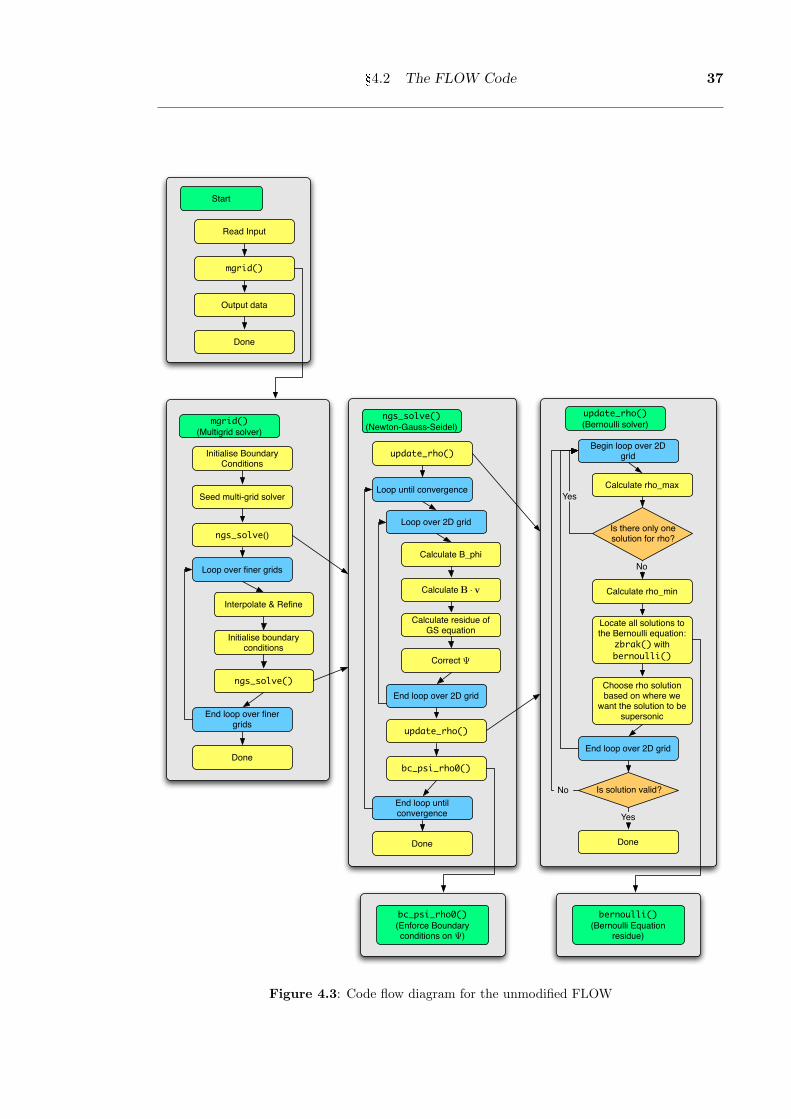
§4.2 The FLOW Code 37
bc_psi_rho0()(Enforce Boundary conditions on !)
ngs_solve()(Newton-Gauss-Seidel)
update_rho()
Calculate B_phi
Calculate B · v
Calculate residue of GS equation
Correct !
Loop over 2D grid
Loop until convergence
End loop over 2D grid
update_rho()
bc_psi_rho0()
End loop until convergence
Done
mgrid()(Multigrid solver)
Initialise Boundary Conditions
Seed multi-grid solver
ngs_solve()
Interpolate & Refine
Initialise boundary conditions
ngs_solve()
End loop over finer grids
Loop over finer grids
Done
Start
Read Input
mgrid()
Output data
Done
update_rho()(Bernoulli solver)
Begin loop over 2D grid
Calculate rho_max
Is there only one solution for rho?
Yes
Calculate rho_min
No
End loop over 2D grid
Choose rho solution based on where we
want the solution to be supersonic
Is solution valid?No
Done
Locate all solutions to the Bernoulli equation:
zbrak() with bernoulli()
Yes
bernoulli()(Bernoulli Equation
residue)
Figure 4.3: Code flow diagram for the unmodified FLOW

38 Calculating Solutions of the Multi-fluid Grad-Shafranov Equation
0.2 0.4 0.6 0.8 1 1.2 1.40
2
4
6
8
10
12
R [m]
p [kP
a]
!"#$%
&"#$%
'() '(* '(+ '(, - -() -(*
!'(,
!'(+
!'(*
!'()
'
'()
'(*
'(+
'(,!
'(''.
'('-
'('-.
'(')
'(').
'('/
0.2 0.4 0.6 0.8 1 1.2 1.40
0.005
0.01
0.015
0.02
0.025
0.03
0.035
R [m]
!
0.2 0.4 0.6 0.8 1 1.2 1.40
50
100
150
200
250
300
R [m]
v! [km
/s]
(c) (d)
(a) (b)
Figure 4.4: Selected quantities from an example single-fluid calculation from the FLOW codeare shown. The plasma boundary used is that of the MAST experiment. In (a), a contour plot ofthe poloidal magnetic flux in the (R,Z) plane is shown. Plots (b)–(d) show cross-sections throughthe Z = 0 mid-plane of (b) the poloidal magnetic flux, (c) the fluid pressure, and (d) the toroidalvelocity of the plasma.

§4.3 Structural Changes Required in FLOW 39
Solutions to the Bernoulli equation can be investigated graphically by plotting thevarious terms of Eq. (4.19), as shown in Figure 4.5. Because the shape of the graph isindependent of the coefficients of the powers of ρ in Eq. (4.19), there will always be either0, 1 or 2 positive solutions to the Bernoulli equation. If there are zero solutions, then anequilibrium state does not exist, and so the plasma must evolve. If there are two solutions,the physically relevant solution must be chosen. For the most part, this will be the higher-density solution, because in the limit of zero poloidal flow, ζ ′(Ψ) → 0, the first term onthe left hand side of Eq. (4.19) will go to zero, and only the higher-density solution willremain. The lower-density solution only becomes physically relevant if there is a pointin the plasma where the two solutions to the Bernoulli equation become degenerate; thispoint corresponds to a transition from subsonic to supersonic poloidal flow [50]. The fluxsurfaces on one side of this point will have subsonic poloidal flow, while those on the otherside will have supersonic poloidal flow. The physically relevant solution for the subsonicside will still be the higher-density solution, but the physically relevant solution for thesupersonic side will be the lower-density solution.
0 0.2 0.4 0.6 0.8 10
0.005
0.01
0.015
0.02
0.025
0.03
0.035
0.04
!
[arb
itra
ry u
nits]
Figure 4.5: Graphically solving the Bernoulli equation (Eq. (4.19)) for the mass-density ρ. The
green dashed line is H(Ψ)+ 12 (RΩ(Ψ))2, the red line is 1
2
(ζ′(Ψ)ρR |B|
)2
, the blue line is γγ−1σ(Ψ)ργ−1.
The black line is the sum of the red and blue lines. Hence, solutions to the Bernoulli equationoccur where the black line intersects with the green one. Note that the mass-density is normalisedto 1 in this plot.
4.3 Structural Changes Required in FLOW
The system of equations under investigation in this work is very similar to those solvedby the original FLOW code (Eq. (4.14) to Eq. (4.16) on page 35). Rewriting to highlightthe similarities to the equations used in the original FLOW code, our system of equationsis: an equation for the toroidal component of the magnetic field (Eq. (3.77) on page 30),
BφR =f(Ψ) + µ0
∑j R2ζ ′j(Ψ)Ωj(Ψ)
1− µ0∑
j1ρj
ζ ′2j (Ψ), (4.20)

40 Calculating Solutions of the Multi-fluid Grad-Shafranov Equation
the Bernoulli equation (Eq. (3.68) on page 28),
Hj(Ψ) =12
(ζ ′j(Ψ)
ρj|B|)2
+γj
γj − 1σj(Ψ)ργj−1
j − 12
(RΩj(Ψ))2 , (4.21)
and the Grad-Shafranov equation (Eq. (3.70) on page 28),
1µ0∇ ·
1− µ0
∑j
1ρj
ζ ′2j
∇ΨR2
=−∑
j
ρjH′j −
∑j
ρjvj,φRΩ′j +
∑j
ργj
j
γj − 1σ′j
− 1µ0
Bφ
Rf ′ −B ·
∑j
vjζ′′j .
(4.22)
As can be seen, the systems of equations are very similar, and only minor structuralchanges were required to FLOW to solve this system. Specifically, instead of solving theBernoulli equation once per grid point, it must be solved once for each fluid at each gridpoint. Additionally, the different summed quantities needed to be calculated to determinethe residue of the Grad-Shafranov equation. These differences are illustrated in Figure 4.6on the facing page.
Although only minor structural changes were necessary, larger technical changes wererequired to enable FLOW to support the multiple fluids and the additional parameters,inputs and outputs for each fluid.
An example multi-fluid solution from the modified FLOW code is shown in Figure 4.7.
4.4 Parameterising the Solution
The system of equations solved by FLOW includes a number of freely specifiable fluxfunctions: ζj(Ψ), Ωj(Ψ), σj(Ψ), Hj(Ψ) and f(Ψ). As most of these functions do notcorrespond naturally to physical quantities, it is not clear how to specify these functions.The approach taken in FLOW (following [50]) is to define a new series of functions thatcorrespond to physical variables in the limit of zero mean fluid velocity and infinite as-pect ratio. In this way, physical intuition can be brought to bear when specifying thesequasi-physical variables. The quasi-variables and their meanings are shown in Table 4.1;these include mass-density, pressure, and the toroidal component of the magnetic field.Additionally, two variables are used to define the toroidal and poloidal flow of the plasma.The poloidal mach number Mj,θ(Ψ) is defined by
Mj,θ(Ψ) =|vpoloidal|
cj,sound,poloidal, (4.23)
where cj,sound,poloidal is the poloidal sound speed for the jth fluid, which itself is given by
cj,sound,poloidal = cj,sound|Bpoloidal||B|
=√
γjpj
ρj
|Bpoloidal||B|
. (4.24)
The toroidal mach number Mj,φ(Ψ) is defined by
Mj,φ(Ψ) = Mj,θ(Ψ) +vj,φ
cj,sound= Mj,θ(Ψ) + vj,φ
√ρj
γjpj. (4.25)

§4.4 Parameterising the Solution 41
ngs_solve()(Newton-Gauss-Seidel)
update_rho()
Calculate B_phi
Calculate B · v
Calculate residue of GS equation
Correct !
Loop over 2D grid
Loop until convergence
End loop over 2D grid
update_rho()
bc_psi_rho0()
End loop until convergence
Done
(a)ngs_solve()
(Newton-Gauss-Seidel)
Loop over 2D grid
Loop until convergence
End loop over 2D grid
update_rho()
bc_psi_rho0()
End loop until convergence
Done
Loop over n fluids
Loop over n fluids
update_rho()
Loop over n fluids
Loop over n fluids
Correct !
Calculate residue of GS equation
Calculate B_phi
Calculate various summed quantities
(b)
Figure 4.6: Structural changes in the function ngs solve() of FLOW. (a) Code flow diagramfor the original ngs solve(). (b) Code flow diagram for the modified ngs solve().

42 Calculating Solutions of the Multi-fluid Grad-Shafranov Equation
0.2 0.4 0.6 0.8 1 1.2 1.4 1.60
5
10
15
20
25
R [m]
p [
kP
a]
Fluid 1
Fluid 2
Total
!"#$%
&"#$%
'() '(* '(+ '(, - -() -(*
!'(,
!'(+
!'(*
!'()
'
'()
'(*
'(+
'(,!
'(''.
'('-
'('-.
'(')
'(').
'('/
'('/.
'('*
0.2 0.4 0.6 0.8 1 1.2 1.4 1.60
0.005
0.01
0.015
0.02
0.025
0.03
0.035
0.04
0.045
R [m]
!
0.2 0.4 0.6 0.8 1 1.2 1.4 1.60
50
100
150
200
250
300
350
400
R [m]
v! [
km
/s]
Fluid 1
Fluid 2
(c) (d)
(a) (b)
Figure 4.7: Selected quantities from an example two-fluid calculation from the modified FLOWcode are shown. The plasma boundary is that of the MAST experiment. In (a), a contour plot ofthe poloidal magnetic flux in the (R,Z) plane is shown. Plots (b)—(d) show cross-sections throughthe Z = 0 mid-plane of (b) the poloidal magnetic flux, (c) the fluid pressure, and (d) the toroidalvelocity of the plasma.

§4.5 Scaling Relationships 43
The definitions of the old flux functions in terms of the new ones are shown in Table 4.2.Note that R0 is the location of the geometric axis, i.e. the centre of the plasma boundary.
Function Physical meaning
Dj(Ψ) Mass densityPj(Ψ) PressureB0(Ψ) Toroidal component of the magnetic field
Mj,θ(Ψ) Poloidal sonic Mach numberMj,φ(Ψ) Toroidal sonic Mach number
Table 4.1: Quasi-variables defined by FLOW
Function Definition
f(Ψ) R0B0(Ψ)ζ ′j(Ψ)
√γjPj(Ψ)Dj(Ψ)Mj,θ(Ψ)
B0(Ψ)
Ωj(Ψ)√
γjPj(Ψ)Dj(Ψ)
Mj,φ(Ψ)−Mj,θ(Ψ)R0
Hj(Ψ) γjPj(Ψ)Dj(Ψ)
(1
γj−1 + Mj,θ(Ψ)Mj,φ(Ψ)− 12M2
j,φ(Ψ))
σj(Ψ) Pj(Ψ)
[Dj(Ψ)]γj
Table 4.2: Definitions of the old flux variables in terms of the new quasi-variables shown inTable 4.1
These quasi-variables can be specified at runtime either through a function parameter-isation or through numerical input as a function of Ψ/Ψmax where Ψmax is the maximumvalue of Ψ.
4.5 Scaling Relationships
Scaling relationships are transformations that leave a system of equations unchanged.These relationships can be used to apply one set of numerical results to a different situ-ation, or (as is useful in numerical calculations) to normalise some quantities to 1 beforecomputation. Normalisation reduces the effect of round-off errors caused by some opera-tions on very large or very small numbers. For example, round-off errors can be significantwhen subtracting large numbers differing only by a small amount. Once the computationis completed with the scaled input quantities, the output can be appropriately scaled togive the correct results for the original input quantities.
The system of equations describing the plasma equilibrium (Eq. (4.20) to Eq. (4.22))have two scaling relationships. If the transformed variables are marked by a tilde (˜), thefirst scaling relationship can be written as:
Ωj →1kj
Ωj , Hj →1k2
j
Hj , ρj → k2j ρj , ζj → kj ζj ,
σj →1
k2γj
j
σj , vj →1kj
vj , pj → pj ,
B→ B, f → f , Ψ→ Ψ,
(4.26)

44 Calculating Solutions of the Multi-fluid Grad-Shafranov Equation
where kj are a set of independent scaling constants. This scaling relationship can beused to normalise the maximum mass-density for each fluid to 1. Because it is not possibleto specify the total plasma mass before the system of equations is solved, this scalingrelationship can be used to scale the solution to match a certain total plasma mass bychoosing appropriate values for the kj.
The second scaling relationship is:
Ωj → Ωj , Hj → Hj , ρj → l2ρj , ζj → l2ζj ,
σj →1
l2(γj−1)σj , vj → vj , pj → l2pj ,
B→ lB, f → lf , Ψ→ lΨ,
(4.27)
where l is the second scaling constant. Because Ψ is not invariant under this transforma-tion, this scaling relationship can only be applied when the functions f(Ψ), ζj(Ψ), Ωj(Ψ),Hj(Ψ), and σj(Ψ) do not depend on the actual value of Ψ, but rather only on the fractionΨ/Ψmax. This is a restriction on the class of functions permissible for the flux functions,but it is a sensible restriction: the order of magnitude of Ψ cannot be known before a calcu-lation except from the results of a similar calculation, or an approximation. It makes senseto parameterise the flux functions in terms of the normalised flux: Ψ/Ψmax. This scalingrelationship is not used in this work because the magnetic field of typical experimentaldevices is of order 1 T, and so normalisation is unnecessary for the magnetic field, andnormalising another quantity would only come at the expense of the already normalisedmagnetic field.
Scaling relationships can also be used to absorb constants into other variables. Forexample, a transformation can be applied to enable the magnetic permeability µ0 = 4π×10−7 H.m−1 to be set to 1. The transformation that enables this is:
Ωj → Ωj , Hj → Hj , ρj →1µ0
ρj , ζj →1µ0
ζj ,
σj → µγj−10 σj , vj → vj , pj →
1µ0
pj ,
B→ B, f → f , Ψ→ Ψ.
(4.28)
Combining the three scaling relationships gives:
Ωj →1kj
Ωj , Hj →1k2
j
Hj , ρj →k2
j l2
µ0ρj , ζj →
kjl2
µ0ζj ,
σj →µ
γj−10
k2γj
j l2(γj−1)σj , vj →
1kj
vj , pj →l2
µ0pj ,
B→ lB, f → lf , Ψ→ lΨ.
(4.29)
4.6 CHEASE [51] Benchmark
In this section, the results of the modified FLOW are compared against the code CHEASE.The CHEASE code was designed for use in reconstructing plasma equilibria, and has beenused in the experiments JET, START, and MAST. For this comparison, the results fromthe modified FLOW were compared against the CHEASE reconstructed equilibrium from

§4.6 CHEASE Benchmark 45
MAST shot #7085 at 290ms. The input files for FLOW were obtained by transformingthe profiles for P (Ψ) and f(Ψ) from the inputs for CHEASE, and setting the variablescontrolling the flow, Mj,φ(Ψ) and Mj,θ(Ψ) to zero because CHEASE does not consider theeffects of either toroidal or poloidal flow.
The boundary of the plasma is specified in terms of a Fourier decomposition R(θ) andZ(θ). The fit used is shown in Figure 4.8(a). The results from FLOW were obtained witha grid of 513× 513 points. A comparison of the results from FLOW against CHEASE areshown in Figure 4.8.
0 0.5 1 1.5!1
!0.8
!0.6
!0.4
!0.2
0
0.2
0.4
0.6
0.8
R [m]
Z [m
]
0
0.005
0.01
0.015
0.02
0.025
0.03
!
0.2 0.4 0.6 0.8 1 1.2 1.4!1
!0.5
0
0.5
1
1.5
2
R [m]
"!
× 1
0!4
0
1
2
3
4
5
6
7
8
9
10
p ×
103 [P
a]
0.2 0.4 0.6 0.8 1 1.2 1.4!1
!0.8
!0.6
!0.4
!0.2
0
0.2
0.4
0.6
0.8
1
R [m]
! p
[Pa]
0.395
0.396
0.397
0.398
0.399
0.4
0.401
0.402
0.403
0.404
0.405
f = B
! R
0.2 0.4 0.6 0.8 1 1.2 1.4!5
!4
!3
!2
!1
0
1
2
3
4
5
R [m]
" f ×
10!5
(a) (b)
(c) (d)
Figure 4.8: The results of the benchmark of the modified FLOW code against CHEASE. The sizeof the final grid used in FLOW was 513× 513. (a) The boundaries used in FLOW and CHEASE.The red line is the boundary used in FLOW, while the blue line is the boundary used by CHEASE,and is mostly hidden by the red line. The Fourier decomposition of the boundary for FLOW isindicated by the circle. Each of (b)–(d) plot a quantity and the discrepancy in this quantitybetween the results of FLOW and CHEASE (calculated as FLOW − CHEASE). The quantityitself is shown in left with its scale being shown on the left of each plot, whilst the discrepancy isshown in red with its scale on the right of each plot. The quantities shown are (b) the poloidalflux , Ψ, (c) the fluid pressure, and (d) the flux function f(Ψ) = BφR.
If the results from FLOW and CHEASE for any of the quantities in Figure 4.8 wereplotted on the same graph, the two lines would be indistinguishable. Consequently, inFigure 4.8(b,c,d), the difference in the results of FLOW and CHEASE are plotted insteadof simply the results from both codes. Of the three plots Figure 4.8(b,c,d), the comparisonof Ψ is the most important as both p and BφR become flux functions in the limit of
46 Calculating Solutions of the Multi-fluid Grad-Shafranov Equation
vanishing flow. For Ψ, the error is less than 1% (excluding a small region around the edgeof the plasma where Ψ is small), indicating excellent agreement between the results fromFLOW and CHEASE. The fluid pressure and BφR also show excellent agreement, havingerrors less than 0.07% and 0.01% respectively.
Two-dimensional plots of the output of FLOW are shown in Figure 4.9 on the facingpage. Figure 4.9(d) shows that the most significant fractional errors in the solution arejust where they would be expected to be: at the edge of the plasma where Ψ is small.
4.7 Multi-fluid Benchmark
As there does not currently exist a code other than the modified form of FLOW that solvesthe multi-fluid model described in this thesis, it is not possible to benchmark the multi-fluid capability of this code against another. However, FLOW can be used to calculatea multi-fluid equilibrium that analytically reduces to a single-fluid equilibrium, and thenthese results can be compared. One way to do this is to decompose a fluid into a numberof fluids that together make up the original. The profiles of the input quantities for eachof these fluids will be the same, but will have different scaling factors. In this section,we decompose the fluid into three separate fluids representing 20%, 30% and 50% of theoriginal fluid. Note that in the presence of flow, the process is not, in general, possible;an arbitrary multi-fluid equilibrium cannot necessarily be reduced to a single-fluid one.
The input used for this comparison is the same as used in the previous section, howeverwith some poloidal and toroidal flow added to ensure that the multi-fluid results reduce tothe single-fluid results even in the presence of flow. The most obvious quantity to comparebetween the single- and multi-fluid cases is the poloidal flux Ψ, as that is the quantity thatis directly solved. The results of the single-fluid and multi-fluid comparison are shown inFigure 4.10.
The comparison between the results is most easily made by comparing the fractionaldifference between the results shown in Figure 4.10(b) to the fractional correction to Ψthat would be made in the next iteration shown in Figure 4.10(c). Because the scalefor these two figures are the same, it is clear that the fractional difference in the resultsfor Ψ is either of the same order of magnitude as the fractional correction to Ψ at thenext iteration, or significantly less (particularly at the edges). While one might haveexpected the fractional difference to be of the order of the fractional correction, howeverit is noted that the difference is significantly less than this at the edges. This is becauseboth calculations converged after the same number of iterations.

§4.7 Multi-fluid Benchmark 47
R [m]
Z [m
]
0.2 0.4 0.6 0.8 1 1.2 1.4
!0.8
!0.6
!0.4
!0.2
0
0.2
0.4
0.6
0.8
! ×
10!
3
5
10
15
20
25
(a)
R [m]
Z [m
]
0.2 0.4 0.6 0.8 1 1.2 1.4
!0.8
!0.6
!0.4
!0.2
0
0.2
0.4
0.6
0.8
p ×
103 [P
a]
1
2
3
4
5
6
7
8
9(b)
R [m]
Z [m
]
! ×
10!
2
0.2 0.4 0.6 0.8 1 1.2 1.4
!0.8
!0.6
!0.4
!0.2
0
0.2
0.4
0.6
0.8
!12
!10
!8
!6
!4
!2
0
2
4
6(c)
R [m]
Z [m
]
0.2 0.4 0.6 0.8 1 1.2 1.4
!0.8
!0.6
!0.4
!0.2
0
0.2
0.4
0.6
0.8
!"
/" ×
10!
5
2
4
6
8
10
(d)
Figure 4.9: Contour plots of selected results from FLOW corresponding to the equilibrium shownin Figure 4.8. The results were computed on a grid of 513 × 513 points. On each plot, the blackline shows the boundary of the plasma. The contours shown are: (a) the poloidal flux, Ψ, (b) thefluid pressure, (c) the residue of the Grad-Shafranov equation, ∆ (see Eq. (4.17) on page 36), and(d) the correction to Ψ at the next iteration as a fraction of Ψ (see Eq. (4.12) on page 33). Thislast plot gives an estimate of the fractional error in the solution to Ψ.

48 Calculating Solutions of the Multi-fluid Grad-Shafranov Equation
R [m]
Z [m
]
!"
× 1
0!7
0.2 0.4 0.6 0.8 1 1.2 1.4
!0.8
!0.6
!0.4
!0.2
0
0.2
0.4
0.6
0.8
!0.5
0
0.5
1
1.5
2
2.5
3
3.5
(a)
R [m]
Z [m
]
0.2 0.4 0.6 0.8 1 1.2 1.4
!0.8
!0.6
!0.4
!0.2
0
0.2
0.4
0.6
0.8
!"
/" ×
10!
4
0
1
2
3
4
5
6
7
8
9
(b)
R [m]
Z [m
]
Frac
tiona
l erro
r in !
(× 1
0!4 )
0.2 0.4 0.6 0.8 1 1.2 1.4
!0.8
!0.6
!0.4
!0.2
0
0.2
0.4
0.6
0.8
0.5
1
1.5
2
2.5
3
3.5
4
4.5
5(c)
Figure 4.10: The results of the multi-fluid benchmark of the modified FLOW code. In this plot,∆Ψ = Ψsingle fluid − Ψthree fluids. The results were computed on a grid of 257 × 257 points. Thecontour plots shown are: (a) the difference between Ψ for the single- and multi-fluid calculations,(b) the difference shown in (a) as a fraction of Ψ, and (c) the correction to Ψ at the next iteration(for the single-fluid calculation) as a fraction of Ψ (see Figure 4.9(d)).

Chapter 5
Numerical Scans
In this chapter, we investigate the effects of an energetic component of a plasma on itsequilibrium. This is done by considering a two-fluid plasma comprising a ‘background’fluid having the greater mass, while the other fluid is the ‘energetic’ component, withgreater toroidal and poloidal velocity.
In the first set of parameter scans, the effect on the plasma equilibrium of the energeticfluid will be investigated by adjusting the pressure and rotational flow of the energetic fluid,while keeping the properties of the background fluid fixed. Different regimes are exploredby varying the magnitude of the appropriate quasi-variables subject to the constraint thatthe total mass of each fluid remain fixed.
In the second set of parameter scans, the robustness of the equilibrium to variationsin the uncertainties in the profile information is explored. In modern fusion experimentssuch as MAST & NSTX, the pressure, density and flow profiles are well resolved for the‘background’ plasma, however this information is not as well known for the ‘energetic’fluid. Additionally, although the total toroidal current can be measured accurately, thecurrent profile is not as well resolved.
5.1 Plasma Performance Measures
In the scans undertaken in this chapter, a range of plasma performance parameters areemployed to describe the changes to the plasma equilibrium. These include differentmeasures of plasma β, the Shafranov shift, and the safety factor. We describe each ofthese in this section.
5.1.1 Plasma β
Arguably, the most important performance measure is the plasma β, which is a measureof the efficiency of the confinement of the plasma pressure by the magnetic field [19, p115]. At each point in the plasma, β is defined by
β =p
|B|2 /(2µ0). (5.1)
Because β is a local quantity, in order to gauge the performance of the entire plasma, an‘average’ β will be necessary. In experimental plasma physics, two such average β’s areoften quoted: the normalised-β, βN , and the poloidal-β, βpoloidal. In this chapter, bothare considered. We extend the definitions of these quantities to be defined for each fluidindividually, labelled by the usual subscript j.
49

50 Numerical Scans
The normalised-β, βN , was devised as an average β whose value can be directly com-pared between different tokamak experiments. The normalised-β is defined by
βj,N =%βj
Iplasma/(aBφ,vacuum), (5.2)
where Iplasma is the total current flowing through the plasma toroidally, a is the minorradius, Bφ,vacuum is the vacuum toroidal magnetic field at the geometric axis, and %βj isdefined by
%βj = 100∫
pjdV/∫
dV
(Bφ,vacuum)2 /(2µ0). (5.3)
The poloidal-β, βpoloidal is a measure of the contribution of the toroidal magnetic fieldcontributes to confining the plasma pressure [19, p 116]. For βpoloidal > 1, the toroidalmagnetic field contributes to confining the plasma, however if βpoloidal < 1, the toroidalmagnetic field displaces some of the plasma pressure. The poloidal β, is defined by
βj,poloidal =∫
pjdS/∫
dS
B2a/(2µ0)
, (5.4)
where Ba is
Ba =µ0Iplasma
l, (5.5)
where l is the perimeter of the plasma cross-section.
Apart from constants, there are only two differences between βj,N and βj,poloidal: βj,N
is proportional to 1/Iplasma and involves the volume-averaged pressure, while βj,poloidal
is proportional to 1/(Iplasma)2 and involves the cross-section-averaged pressure. Withregards to the pressures, this means that if the pressure profile shifts outboard, the volume-averaged pressure is likely to increase (because dV = 2πR dR dZ), while the cross-section-averaged pressure is likely to remain approximately constant (because dS = dR dZ).
5.1.2 Shafranov Shift, ∆S
Another measure of the plasma equilibrium is the distance between the magnetic axis (thelocation where Ψ has its maximum), and the geometric axis (the centre of the plasmaboundary). This distance is known as the Shafranov shift,
∆S =√
(Rmag −R0)2 + (Zmag − Z0)
2, (5.6)
where (Rmag, Zmag) is the location of the magnetic axis, and (R0, Z0) is the location of thegeometric axis.
5.1.3 Safety Factor, q
The safety factor (so-called because small values of the safety factor are related to in-stabilities in the plasma) is the number of toroidal orbits a magnetic field line makes foreach poloidal orbit. Because magnetic field lines are restricted to surfaces of constant Ψ(because the poloidal magnetic field follows contours of constant Ψ), the safety factor is a

§5.2 Physics Studies 51
function of Ψ. The safety factor, q(Ψ) is defined by
q(Ψ) =12π
∮1R
Bφ
|Bpoloidal|dl, (5.7)
where dl is an element of length along a surface of constant Ψ. Because this integralcannot be carried out for Ψ = Ψmax, the value of the safety factor at the magnetic axis isthe limit of this integral as Ψ→ Ψmax.
5.2 Physics Studies
In this section the physical effects of varying the magnitude of the profiles describing theenergetic fluid is investigated while keeping the properties of the background fluid, and thetotal mass of each fluid, constant. First, a profile parameterisation for the quasi-variablesis chosen, and the constraints of the parameterisation are given. Finally, we discuss theresults of the scans of the toroidal quasi-Mach number Mj,φ, the poloidal quasi-Machnumber Mj,θ, and the quasi-pressure Pj . A scan of the quasi-density Dj is unnecessary asthe scan would not conserve the total mass of the energetic fluid.
5.2.1 Profile Parameterisations
In order to explore the physics of the energetic species, profiles must be chosen for thequasi-variables defining the energetic fluid. In this section, we follow Guazzotto et al. [5]and use a power-law expression for parameterising the quasi-variables. The parameterisa-tions used are:
Pj(Ψ) = Pj,edge + (Pj,centre − Pj,edge)∣∣∣∣ ΨΨmax
∣∣∣∣2 , (5.8)
Dj(Ψ) = Dj,edge + (Dj,centre −Dj,edge)∣∣∣∣ ΨΨmax
∣∣∣∣ 12 , (5.9)
Mj,φ(Ψ) = Mj,φ,max
(∣∣∣∣ ΨΨmax
∣∣∣∣+ Mj,φ,min
) 12
, (5.10)
Mj,θ(Ψ) =
Mj,θ,edge at the plasma boundary (Ψ = 0)
4Mj,θ,max
∣∣∣∣ ΨΨmax
∣∣∣∣ (1−∣∣∣∣ ΨΨmax
∣∣∣∣) otherwise,
(5.11)
where Ψmax is the maximum value of Ψ (i.e. the value of Ψ at the magnetic axis), Pj is thequasi-pressure, Dj is the quasi-density and Mj,φ and Mj,θ are the toroidal and poloidalquasi-Mach numbers respectively. The parameterisations for Pj and Dj are used only forthe energetic fluid as experimental data was available for the pressure and density of thebackground fluid from MAST. However, the parameterisations for Mj,φ and Mj,θ are usedfor both fluids in the absence of toroidal and poloidal flow data from MAST.
5.2.2 Constraints
In this section, the profiles of the quantities in Eq. (5.8) to Eq. (5.11) will be kept constant,and only their magnitudes will be varied. This is partly done to reduce the number of
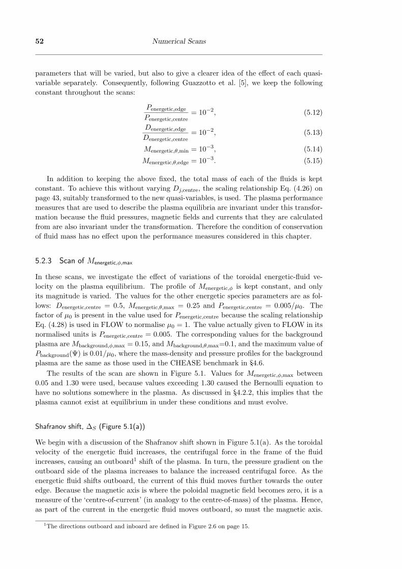
52 Numerical Scans
parameters that will be varied, but also to give a clearer idea of the effect of each quasi-variable separately. Consequently, following Guazzotto et al. [5], we keep the followingconstant throughout the scans:
Penergetic,edge
Penergetic,centre= 10−2, (5.12)
Denergetic,edge
Denergetic,centre= 10−2, (5.13)
Menergetic,θ,min = 10−3, (5.14)
Menergetic,θ,edge = 10−3. (5.15)
In addition to keeping the above fixed, the total mass of each of the fluids is keptconstant. To achieve this without varying Dj,centre, the scaling relationship Eq. (4.26) onpage 43, suitably transformed to the new quasi-variables, is used. The plasma performancemeasures that are used to describe the plasma equilibria are invariant under this transfor-mation because the fluid pressures, magnetic fields and currents that they are calculatedfrom are also invariant under the transformation. Therefore the condition of conservationof fluid mass has no effect upon the performance measures considered in this chapter.
5.2.3 Scan of Menergetic,φ,max
In these scans, we investigate the effect of variations of the toroidal energetic-fluid ve-locity on the plasma equilibrium. The profile of Menergetic,φ is kept constant, and onlyits magnitude is varied. The values for the other energetic species parameters are as fol-lows: Denergetic,centre = 0.5, Menergetic,θ,max = 0.25 and Penergetic,centre = 0.005/µ0. Thefactor of µ0 is present in the value used for Penergetic,centre because the scaling relationshipEq. (4.28) is used in FLOW to normalise µ0 = 1. The value actually given to FLOW in itsnormalised units is Penergetic,centre = 0.005. The corresponding values for the backgroundplasma are Mbackground,φ,max = 0.15, and Mbackground,θ,max=0.1, and the maximum value ofPbackground(Ψ) is 0.01/µ0, where the mass-density and pressure profiles for the backgroundplasma are the same as those used in the CHEASE benchmark in §4.6.
The results of the scan are shown in Figure 5.1. Values for Menergetic,φ,max between0.05 and 1.30 were used, because values exceeding 1.30 caused the Bernoulli equation tohave no solutions somewhere in the plasma. As discussed in §4.2.2, this implies that theplasma cannot exist at equilibrium in under these conditions and must evolve.
Shafranov shift, ∆S (Figure 5.1(a))
We begin with a discussion of the Shafranov shift shown in Figure 5.1(a). As the toroidalvelocity of the energetic fluid increases, the centrifugal force in the frame of the fluidincreases, causing an outboard1 shift of the plasma. In turn, the pressure gradient on theoutboard side of the plasma increases to balance the increased centrifugal force. As theenergetic fluid shifts outboard, the current of this fluid moves further towards the outeredge. Because the magnetic axis is where the poloidal magnetic field becomes zero, it is ameasure of the ‘centre-of-current’ (in analogy to the centre-of-mass) of the plasma. Hence,as part of the current in the energetic fluid moves outboard, so must the magnetic axis.
1The directions outboard and inboard are defined in Figure 2.6 on page 15.

§5.2 Physics Studies 53
0 0.2 0.4 0.6 0.8 1 1.2 1.40.11
0.12
0.13
0.14
0.15
0.16
0.17
0.18
0.19
Shaf
rano
v sh
ift [m
]
Menergetic,!,max0 0.2 0.4 0.6 0.8 1 1.2 1.40.8
1
1.2
1.4
1.6
1.8
On!
axis
safe
ty fa
ctor
q0
Menergetic,!,max
0 0.2 0.4 0.6 0.8 1 1.2 1.40
0.5
1
1.5
2
2.5
3
3.5
4
4.5
Menergetic,!,max
Plas
ma " N Background plasma "N
High energy species "NTotal plasma "NReference "N
0 0.2 0.4 0.6 0.8 1 1.2 1.40
0.5
1
1.5
Menergetic,!,max
Plas
ma " po
l Background plasma "polHigh energy species "polTotal plasma "polReference "pol
(a) (b)
(c) (d)
Figure 5.1: Selected plasma properties vs. energetic toroidal Mach number, Menergetic,φ,max.Each equilibrium calculated on a 257× 257 grid. The four plots show (a) the Shafranov shift, ∆S
(separation of the magnetic and geometric axes), (b) the on-axis value of the safety factor, q0, (c)the normalised-β, βN , and (d) the poloidal-β, βpoloidal. The ‘reference’ β’s referred to in plots (c)and (d) are the values of the respective β’s for the plasma equilibrium with the background plasmaonly. The value of Mφ,max for the background fluid is 0.15.

54 Numerical Scans
We note that the step increments in Figure 5.1(a) correspond to the radial grid resolutionused in FLOW.
Safety factor at the magnetic axis, q0 (Figure 5.1(b))
The value of the safety profile at the magnetic axis depends inversely upon the magnitudeof the poloidal magnetic field near the magnetic axis, as shown by Eq. (5.7). Near themagnetic axis, an approximation for |Bpoloidal| can be made from Ampere’s law. Considera small Amperian loop along a contour of constant Ψ (i.e. parallel to the poloidal magneticfield) near the magnetic axis. Ampere’s law gives∮
Bpoloidal · dl =∮|Bpoloidal| dl = µ0
∫JφdA, (5.16)
where dl is the element of length along a contour of constant Ψ. Sufficiently close to themagnetic axis, this contour will approximate a circle of radius r, and both |Bpoloidal| andJφ will be constant over this circle. Using this approximation, the following relationshipis obtained for the poloidal magnetic field near the magnetic axis:
|Bpoloidal| =12µ0 |Jφ,mag| r, (5.17)
where Jφ,mag is the toroidal current density at the magnetic axis. Substituting this ex-pression into Eq. (5.7), and applying the same approximation gives
q0 =2 |Bφ,mag|
µ0 |Jφ,mag|Rmag, (5.18)
where Bφ,mag is the value of the toroidal magnetic field at the magnetic axis. Because thetoroidal magnetic field is mostly determined by the vacuum toroidal field, q0 is principallya measure of the toroidal current density at the magnetic axis, and the location of themagnetic axis through Rmag.
An expression for JφR at the magnetic axis can be obtained by using a straight-forwardgeneralisation of Eq. (3.30) on page 22,
Jφ = − 1µ0
R∇ ·(
1R2∇Ψ
). (5.19)
Combining this with the generalised Grad-Shafranov equation (Eq. (6.3) on page 69) andnoting that ζ ′j → 0 at the magnetic axis, JφR at the magnetic axis can be written as
JφR =R2∑
j
ρjH′j + R4
∑j
ρjΩjΩ′j +
1µ0
ff ′ + R2f∑
j
Ω′jζ
′′j −R2
∑j
ργj
j
γj − 1σ′j , (5.20)
where all variables are evaluated at the magnetic axis, and f(Ψ) = BφR because ζ ′j = 0.
The behaviour of q0 in Figure 5.1(b) can be explained through examining the depen-dence of Eq. (5.20) on Mj,φ. Substitution of the quasi-variable definitions in Table 4.2on page 43 into Eq. (5.20), reveals that JφR at the magnetic axis has a combination of a

§5.2 Physics Studies 55
linear and a quadratic dependence on Mj,φ,max. That is,
Jφ ∝∑
j
R2γjPjM
′j,θ
[1 +
ρj
Dj
(1− R2
R20
)]Mj,φ
+∑
j
[12R2
(R2
R20
− 1)
γjρj
(Pj
Dj
)′]Mj,φM ′
j,φ,
(5.21)
where M ′j,φ ∝ Mj,φ,max, and all variables are evaluated at the magnetic axis. For suf-
ficiently small Mj,φ,max, the linear term will dominate the dependence of JφR at themagnetic axis, but as Mj,φ,max increases the quadratic term will dominate. The linearterm acts to decrease JφR, while the quadratic term increases it. This is because at the
magnetic axis, M ′j,θ < 0 from Eq. (5.11) on page 51, ρj
Dj∼ 1, 0 <
(R2
R20− 1)
. 0.5, and
0 <(
Pj
DjM2
j,φ
)′.
As can be seen from Figure 5.1(b), for Menergetic,φ,max . 0.2, the linear term dominatesand JφR at the magnetic axis decreases. Because the on-axis value of the safety profile q0
is inversely proportional to JφR at the magnetic axis, as Menergetic,φ,max increases, q0 willalso increase up to Menergetic,φ,max ∼ 0.2. After this point, the quadratic term begins todominate, and at the magnetic axis, JφR begins to increase, hence decreasing q0.
Plasma β (Figure 5.1(c,d))
The behaviour of the two average β’s in Figure 5.1(c,d) is more complex. Qualitatively, theenergetic fluid’s mass-density profile shifts outboard (even more than the magnetic axis),and also heightens and narrows as Menergetic,φ increases. In turn, this has a similar effecton the pressure profile of the energetic fluid (as shown in Figure 5.2), and so the energeticfluid’s β’s are increased. The pressure of the background plasma is not increased, but itsprofile is shifted outboard due to the shift of the magnetic axis. This has little effect onthe average background fluid pressure used for either βN or βpoloidal. The reduction in theβ’s for the background plasma comes from an increase in the total toroidal plasma currentcaused by the increased velocity of the energetic fluid.
To explain the cause for the change in the pressure profile of the energetic fluid asMenergetic,φ,max is increased, an exact solution for the fluid-mass density is first obtained inthe limit of small poloidal flow. Substituting this approximate expression into Eq. (3.54)on page 25 will enable an approximate solution to be obtained for the pressure, pj , fromwhich its dependence upon Mj,φ,max can be investigated.
An approximate dependence of ρj on Mj,φ,max is found by obtaining an approximatesolution for ρj from the Bernoulli equation. Near the magnetic axis, the poloidal flowwill be small (as shown by Eq. (5.11)), and the first term on the right hand side of theBernoulli equation (Eq. (3.77) on page 30) can be neglected. This gives
ρj ≈
γj − 1γjσj(Ψ)
[Hj(Ψ) +
12
(RΩj(Ψ))2] 1
γj−1
, (5.22)
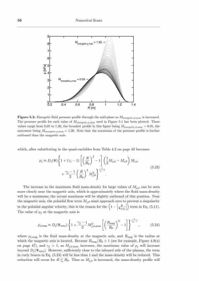
56 Numerical Scans
0.2 0.4 0.6 0.8 1 1.2 1.40
1
2
3
4
5
6
7
8
9
p [kP
a]
R [m]
Menergetic,!,max
= 0.05 "
Menergetic,!,max
= 1.30 "
Figure 5.2: Energetic fluid pressure profile through the mid-plane as Menergetic,φ,max is increased.The pressure profile for each value of Menergetic,φ,max used in Figure 5.1 has been plotted. Thesevalues range from 0.05 to 1.30, the broadest profile in this figure being Menergetic,φ,max = 0.05, thenarrowest being Menergetic,φ,max = 1.30. Note that the maximum of the pressure profile is furtheroutboard than the magnetic axis.
which, after substituting in the quasi-variables from Table 4.2 on page 43 becomes
ρj ≈ Dj(Ψ)
1 + (γj − 1)
[(R
R0
)2
− 1
](12Mj,φ −Mj,θ
)Mj,φ
+γj − 1
2
(R
R0
)2
M2j,θ
1γj−1
.
(5.23)
The increase in the maximum fluid mass-density for large values of Mj,φ can be seenmore clearly near the magnetic axis, which is approximately where the fluid mass-densitywill be a maximum; the actual maximum will be slightly outboard of this position. Nearthe magnetic axis, the poloidal flow term Mj,θ must approach zero to prevent a singularity
in the poloidal angular velocity, this is the reason for the(1−
∣∣∣ ΨΨmax
∣∣∣) term in Eq. (5.11).The value of ρj at the magnetic axis is
ρj,mag ≈ Dj(Ψmax)
1 +
γj − 12
M2j,φ,max
[(Rmag
R0
)2
− 1
] 1γj−1
, (5.24)
where ρj,mag is the fluid mass-density at the magnetic axis, and Rmag is the radius atwhich the magnetic axis is located. Because Rmag/R0 > 1 (see for example, Figure 4.9(a)on page 47), and γj > 1, as Mj,φ,max increases, the maximum value of ρj will increasebeyond Dj(Ψmax). However, sufficiently close to the inboard side of the plasma, the termin curly braces in Eq. (5.23) will be less than 1 and the mass-density will be reduced. Thisreduction will occur for R . R0. Thus as Mj,φ is increased, the mass-density profile will

§5.2 Physics Studies 57
be shifted outboard, heightened and narrowed.A similar effect also occurs for the fluid pressure, as can be seen by using the definition
of σj(Ψ) in Eq. (3.54) on page 25 with Eq. (5.24) to solve for the fluid pressure in termsof the quasi-variables in Table 4.2 on page 43,
pj,mag ≈ Pj(Ψ)
1 +
γj − 12
Mj,φ,max
[(Rmag
R0
)2
− 1
] γjγj−1
. (5.25)
Thus, for the same reasons as given before for the fluid mass-density, as Mj,φ is increasedthe pressure profile will be both heightened and narrowed, but even more so than for thefluid mass-density because the exponent of the term in curly braces in Eq. (5.25) is greaterthan the exponent in Eq. (5.24). The heightening and narrowing of penergetic is shown inFigure 5.2.
The increase in the maximum fluid mass-density and pressure at the magnetic axis ispartially an effect of the profile parameterisation: Dj(Ψ) and Pj(Ψ) are the quasi -mass-density and quasi -pressure respectively, they only correspond to ρj and pj in the zero-flow,R0 →∞ limit. By appropriately varying Pj(Ψ) and Dj(Ψ), a scan could be performedwhere Menergetic,φ is increased while keeping either the maximum mass-density constantand/or the maximum pressure constant, or possibly keeping the value of the mass-densityand/or pressure at the magnetic axis constant. Nevertheless, the change in the shape ofthe profile is a physical effect as shown in Eq. (5.22): on a given flux surface (i.e. for fixedΨ), the mass-density (and also the pressure) varies on a flux surface, increasing towardsthe outboard side of the plasma. Importantly, the maximum mass-density and pressureof a fluid will always be outboard of the magnetic axis for non-zero toroidal flow of thatfluid.
In this scan, Mbackground,φ,max is kept constant while Menergetic,φ,max is varied. As aresult, only the energetic fluid’s pressure and mass-density will be heightened and narrowedas Menergetic,φ,max is increased; the pressure and mass-density of the background fluid willonly experience a slight outboard shift due to the shift of the magnetic axis. Because themaximum pressure increases so much more significantly than the pressure profile narrows,both β’s for the energetic fluid increase despite the increasing toroidal plasma current.
5.2.4 Scan of Menergetic,θ,max
Next, we investigate the effect of variations in the poloidal energetic-fluid velocity on theplasma equilibrium. The profile of Menergetic,θ is kept constant, only its magnitude isvaried. The values for the other parameters used for the energetic species are as follows:Denergetic,centre = 0.5, Menergetic,φ,max = 0.7 and Penergetic,centre = 0.005/µ0. The values forthe background plasma are the same as in §5.2.3. The results of the scan are shown inFigure 5.3. Values for Menergetic,θ,max between 0.01 and 0.40 were used, because valuesexceeding 0.40 caused the Bernoulli equation to have no solutions at some point in theplasma. A similar limitation was found in §5.2.3.
Shafranov shift, ∆S (Figure 5.3(a))
Increasing poloidal flow has comparably little effect on the position of the magnetic axisas shown in Figure 5.3(a). This is not unexpected because the increasing poloidal flowwill not add to any outboard centrifugal force in the fluid’s frame of reference.
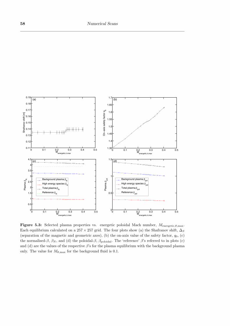
58 Numerical Scans
0 0.1 0.2 0.3 0.4 0.50.11
0.12
0.13
0.14
0.15
0.16
0.17
0.18
0.19
Shaf
rano
v sh
ift [m
]
Menergetic,!,max0 0.1 0.2 0.3 0.4 0.51.35
1.4
1.45
1.5
1.55
1.6
1.65
1.7
On!
axis
safe
ty fa
ctor
q0
Menergetic,!,max
0 0.1 0.2 0.3 0.4 0.50
0.5
1
1.5
2
2.5
3
3.5
4
4.5
Menergetic,!,max
Plas
ma " N Background plasma "N
High energy species "NTotal plasma "NReference "N
0 0.1 0.2 0.3 0.4 0.50
0.5
1
1.5
Menergetic,!,max
Plas
ma " po
l Background plasma "polHigh energy species "polTotal plasma "polReference "pol
(a) (b)
(c) (d)
Figure 5.3: Selected plasma properties vs. energetic poloidal Mach number, Menergetic,θ,max.Each equilibrium calculated on a 257× 257 grid. The four plots show (a) the Shafranov shift, ∆S
(separation of the magnetic and geometric axes), (b) the on-axis value of the safety factor, q0, (c)the normalised-β, βN , and (d) the poloidal-β, βpoloidal. The ‘reference’ β’s referred to in plots (c)and (d) are the values of the respective β’s for the plasma equilibrium with the background plasmaonly. The value for Mθ,max for the background fluid is 0.1.

§5.2 Physics Studies 59
Plasma β (Figure 5.3(c,d))
The steady decline of both β’s for the background and energetic fluids shown in Fig-ure 5.3(c,d) is due to the steady increase of the plasma current with Menergetic,θ,max, asshown in Figure 5.4. It is clear from this figure that for the range of Menergetic,θ,max shown,the dependence of the total current upon Menergetic,θ,max is approximately linear. Withthis in mind, we investigate the dependence of the toroidal current density Jφ on Mj,θ.
! !"# !"$ !"% !"& !"'!"%
!"%!'
!"%#
!"%#'
!"%$
!"%$'
!"%%
!"%%'
()*)+,)-./0!0123
452612789++)*-7:(),2!;1<6=
Figure 5.4: Plasma current as Menergetic,θ,max is increased.
To obtain an expression for the toroidal current density, Eq. (5.19) is solved with thegeneralised Grad-Shafranov equation, Eq. (6.3) on page 69, to arrive at a generalisationof Eq. (5.20):
Jφ =R∑
j
ρjH′j + R3
∑j
ρjΩjΩ′j +
f ′
µ0Bφ + BφR2
∑j
Ω′jζ
′′j
−R∑
j
ργj
j
γj − 1σ′j +
∑j
ζ ′jζ′′j
ρjR
[|∇Ψ|2 + (BφR)2
]−R∇ ·
∑j
1ρj
ζ ′2j∇ΨR2
.
(5.26)
The linear dependence of Jφ upon Mj,θ is mainly present in the fourth term on the RHSof Eq. (5.26) through ζ ′′j , and to a lesser extent in the first term on the RHS throughH ′
j . The dependence of the first term is suppressed compared to the fourth because, once
expanded in terms of the quasi-variables, the first term is found to contain(1− R2
R20
),
which suppresses the first term, whereas the fourth term does not.The linear dependence of Eq. (5.26) with the poloidal flow does not increase the toroidal
current density throughout the entire plasma, but instead only near the plasma boundary,while it instead decreases the current density near the centre of the plasma. This is becauseζ ′′j is proportional to M ′
j,θ, and from the definition of Mj,θ in Eq. (5.11) on page 51, M ′j,θ
is positive only for Ψ < 12Ψmax and becomes negative for Ψ > 1
2Ψmax. However, thenet effect is to increase the total toroidal current because the area of the plasma whereΨ < 1
2Ψmax is approximately twice as large as the area where Ψ > 12Ψmax, as can be seen

60 Numerical Scans
from Figure 4.9(a) on page 47. The more significant reduction in βpoloidal is because ofits dependence on 1/I2
plasma whereas βN is proportional to 1/Iplasma. The pressures areessentially unaffected by the increasing poloidal flow; the effect on the β’s is due entirelyto the increasing total toroidal current.
Safety factor at the magnetic axis, q0 (Figure 5.3(b))
Another consequence of the reduction in current density in the centre of the plasma isthat the value of the safety factor at the magnetic axis increases with increasing poloidalflow as shown in Figure 5.3(b). This is because q0 is inversely proportional to Jφ at themagnetic axis as shown in Eq. (5.18).
The higher density of points between 0.25 . Menergetic,θ,max . 0.30 was to resolve fine-scale structures of the plot of the on-axis safety profile when the grid resolution was129×129 points, however, this mostly disappeared when the grid resolution was increasedto 257× 257 points. It is believed that the slight kink in the on-axis safety profile aroundMenergetic,θ,max ≈ 0.27 is a numerical artefact that would be smoothed if the grid resolutionwas further increased.
5.2.5 Scan of Penergetic,centre
Finally, we investigate the effect of variations in the energetic fluid pressure on theplasma equilibrium. The profile of Penergetic is kept constant, only its magnitude is var-ied. The values for the other parameters used for the energetic species are as follows:Denergetic,centre = 0.5, Menergetic,φ,max = 0.7 and Menergetic,θ,max = 0.25. The correspondingvalues for the background plasma are the same as in §5.2.3 and §5.2.4.
The results of the scan are shown in Figure 5.5, values for Penergetic,centre between5 × 10−4/µ0 and 10−2/µ0 were used. Larger values imply the maximum pressure of theenergetic fluid exceeds that of the background plasma.
Shafranov shift, ∆S (Figure 5.5(a))
Qualitatively, the magnetic axis shifts outboard as the pressure of the energetic fluid isincreased because of an outboard shift in the toroidal current. An outboard shift in thetoroidal current density will hence translate into an outboard shift of the magnetic axis.The cause for this outboard shift in the toroidal current density can be seen by neglectingthe poloidal and toroidal flow in Eq. (5.26), and substituting the definitions of the quasi-variables in Table 4.2 on page 43. This yields
Jφ = R∑
j
P ′j +
1µ0
ff ′
R. (5.27)
This dependence is equivalent the fact that the J×B force balances the force due to thegradient in the pressure, which acts away from the centre of the plasma. If the pressureprofile increases, ∇p will increase, and so the current must also increase for the plasmato remain in equilibrium. The toroidal current also shifts slightly outboard because thedominant contribution to the magnetic field, the toroidal vacuum magnetic field, decreasesas 1
R . To balance the increasing ∇p force, J must increase more towards the outboardside of the plasma. Consequently, the magnetic axis will shift outboard as the pressure ofthe energetic species is increased.

§5.2 Physics Studies 61
0 0.002 0.004 0.006 0.008 0.01 0.0120.11
0.12
0.13
0.14
0.15
0.16
0.17
0.18
0.19
Shaf
rano
v sh
ift [m
]
µ0 Penergetic,centre0 0.002 0.004 0.006 0.008 0.011
1.2
1.4
1.6
1.8
2
2.2
2.4
2.6
On!
axis
safe
ty fa
ctor
q0
µ0 Penergetic,centre
0 0.002 0.004 0.006 0.008 0.010
0.5
1
1.5
2
2.5
3
3.5
4
4.5
µ0 Penergetic,centre
Plas
ma ! N Background plasma !N
High energy species !NTotal plasma !NReference !N
0 0.002 0.004 0.006 0.008 0.010
0.5
1
1.5
µ0 Penergetic,centre
Plas
ma ! po
l
Background plasma !polHigh energy species !polTotal plasma !polReference !pol
(a) (b)
(c) (d)
Figure 5.5: Selected plasma properties vs. central energetic pressure, Penergetic,centre. Eachequilibrium calculated on a 257 × 257 grid. The four plots show (a) the Shafranov shift, ∆S
(separation of the magnetic and geometric axes), (b) the on-axis value of the safety factor, q0, (c)the normalised-β, βN , and (d) the poloidal-β, βpoloidal. The ‘reference’ β’s referred to in plots (c)and (d) are the values of the respective β’s for the plasma equilibrium with the background plasmaonly. The maximum value of the pressure of the background fluid is 0.012/µ0.

62 Numerical Scans
Safety factor at the magnetic axis, q0 (Figure 5.5(b))
The behaviour of the on-axis value of the safety factor in Figure 5.5(b) can be also ex-plained with reference to Eq. (5.27). Because the toroidal current density must increasethroughout the entire plasma to balance the increasing ∇p force, the toroidal currentdensity at the magnetic axis increases. This causes the value of the safety factor at themagnetic axis to decrease as per Eq. (5.18).
Plasma β (Figure 5.5(c,d))
The steady increase in both β’s for the energetic fluid is directly caused by the increasein the pressure of the energetic species, as would be expected. The decrease in the β’s forthe background plasma is due to an increased total toroidal current, caused by a highertoroidal current density throughout the entire plasma as discussed previously.
The total plasma β’s have different behaviours because of their different dependencieson the total toroidal current. Although the energetic fluid’s βpoloidal is increasing, theβpoloidal for the background fluid decreases more rapidly because it is proportional to1/(Iplasma)2 causing the total βpoloidal to decrease. For βN , because it is proportional to1/Iplasma, the total βN increases despite the reduction in βN of the background plasma.
5.3 Equilibrium Sensitivity to Profile Variations
One of the difficulties in tokamak experiments is determining the physical properties ofthe plasma discharge. This problem arises because all measurement equipment mustbe located either outside of the plasma, or at its edge to minimise both disruptions tothe plasma and damage to the measurement device. Although some properties of theplasma can be obtained from these measurements, such as the pressure, density and flowprofiles, other properties, such as the location of the flux surfaces, cannot. This problem ispartially solved by measuring a range of properties of the plasma and using an equilibriumreconstruction code, such as EFIT (described in Table 2.1 on page 16), to repeatedly solvethe Grad-Shafranov equation until the solution is consistent with the measurements.
In many tokamak experiments without a motional Stark effect diagnostic [53] (suchas MAST and NSTX), the greatest source of uncertainty lies in the current profile, andtherefore the location of the internal flux surfaces and the safety-factor profile. A sec-ond source of uncertainty lies in the energetic fluid profiles. Whilst diagnostics do existto characterise the energetic fluid, they are usually less well developed, and at a lowerresolution than their thermal counterparts.
We aim to investigate the effect of variations of the energetic profiles on the plasmaequilibrium. To do this, the current density profile is varied and a new plasma equilibriumis constructed that conserves two experimentally measurable quantities: the total toroidalplasma current Iplasma, and a measure of the total energy of the plasma, Λ, yet to bedefined. These conditions are met by varying the magnitude of the current profile, andthe profile of the energetic fluid’s pressure or toroidal flow. Finally, the sensitivity ofthe poloidal flux Ψ with respect to the changes in the profiles of the energetic fluid isinvestigated.

§5.3 Equilibrium Sensitivity to Profile Variations 63
5.3.1 Profile Parameterisations
To investigate the effect of profile variations, it will be necessary to be able to vary theshape of the pressure and toroidal flow profiles while keeping their maxima constant.This is achieved by allowing the exponents in Eq. (5.8) and Eq. (5.10) to vary. Theparameterisations used for the quasi-density and the quasi-poloidal Mach number in thissection are the same as those given in §5.2.1, while the parameterisations used for thequasi-pressure and quasi-toroidal Mach number of the energetic fluid are:
Pj(Ψ) = Pj,edge + (Pj,centre − Pj,edge)∣∣∣∣ ΨΨmax
∣∣∣∣αP
, (5.28)
Mj,φ(Ψ) = Mj,φ,max
(∣∣∣∣ ΨΨmax
∣∣∣∣+ Mj,φ,min
)αφ
, (5.29)
where in the parameterisation given in §5.2.1, αP = 2, and αφ = 12 .
A mapping is also needed to vary the toroidal current density profile, and while Jφ isnot a flux function, Eq. (5.27) suggests varying f(Ψ). The mapping used is
f
(∣∣∣∣ ΨΨmax
∣∣∣∣) = fCHEASE(0) + λ1
[fCHEASE
(∣∣∣∣ ΨΨmax
∣∣∣∣λ0)− fCHEASE(0)
], (5.30)
where fCHEASE(Ψ/Ψmax) is the profile used in CHEASE, and f(Ψ) is written as a functionof Ψ/Ψmax to be consistent with fCHEASE(Ψ). The magnitude of f(Ψ) must be able tovary in order to ensure that when the current profile is compressed or expanded (λ0 > 1and λ0 < 1, respectively) that the total toroidal current Ip can be preserved. Indeed, theparticular form for the parameterisation of f(Ψ) was chosen to ensure that f(0) remainsconstant when the current profile is varied. This is because at the boundary of the plasmaf(Ψ) = BφR, and Bφ will be the vacuum toroidal magnetic field, a well-determinedparameter.
5.3.2 Constraints
In this section, only the profiles of the quasi-pressure and quasi-toroidal Mach numberwill be varied, and the maxima of these profiles will be kept constant. Consequently, inaddition to the constraints given in §5.2.2, the following are also kept constant:
Penergetic,centre = 0.005/µ0, (5.31)
Denergetic,centre = 0.5, (5.32)
Menergetic,φ,max = 0.7, (5.33)
Menergetic,θ,max = 0.25, (5.34)
where these were the values used for these constants in the scans in Section 5.2.In this section, equilibria will be investigated subject to the conservation of two prop-
erties of the plasma that can be determined experimentally. The first of these is the totaltoroidal plasma current,
Ip =∫
Jφ dA. (5.35)
The other experimentally measurable quantity that will be conserved is a measure ofthe energy of the plasma. In 1971, Shafranov [54] showed that for a plasma equilibrium
64 Numerical Scans
with zero flow, a combination of certain plasma parameters (here denoted by Λ) couldbe written in terms of two integrals over the plasma boundary and a volume integral.Because the contribution of the volume integral to the sum is much less than that of thesurface integrals, the quantity Λ remains robust to variations in the internal structureof the equilibrium while also being experimentally measurable through the properties ofthe plasma at its surface. This expression was generalised to the case of a plasma witharbitrary flow by Lao et al. [55] in 1985. The result obtained by Lao et al. was
βp + Wpt +`i
2= Λ, (5.36)
where βp, Wpt and `i are defined as:
βp =2µ0
B2aV
∫p dV, (5.37)
Wpt =µ0
B2aV
∫ρv2
φ dV, (5.38)
`i =1
B2aV
∫|Bpol|2 dV, (5.39)
with V the plasma volume, and Ba a poloidal magnetic field used for normalisation definedin Eq. (5.5). In this section, we assume without proof a generalisation of Lao et al.’s resultto a multi-fluid equilibrium: ∑
j
βp,j +∑
j
Wpt,j +`i
2= Λ, (5.40)
where
βp,j =2µ0
B2paV
∫pj dV, (5.41)
Wpt,j =µ0
B2paV
∫ρjv
2j,φ dV. (5.42)
Just as in Section 5.2, conservation of plasma mass for each fluid is automaticallysatisfied.
5.3.3 Method
The aim of this section is to investigate the sensitivity of the plasma equilibrium to varia-tions in the profiles of certain properties of the plasma while two experimentally measur-able quantities are conserved. In each scan, the profile of the toroidal current density isperturbed by selecting a value for λ0 6= 1, and values are sought for λ1 and one of the α’s(the other is kept fixed) such that Ip and Λ have the same values as for λ0 = 1, i.e. theunperturbed equilibrium. This is done in two separate scans. In the first, the profile ofthe quasi-pressure is allowed to vary through αP while αφ is kept fixed. In the second, theprofile of the quasi-toroidal Mach number is allowed to vary through αφ, and αP is keptfixed. The values for λ1 and either αP or αφ are sought by using MATLAB’s fminsearch

§5.3 Equilibrium Sensitivity to Profile Variations 65
nonlinear minimisation routine to find values of λ1 and α such that∣∣∣∣∆Ip
Ip0
∣∣∣∣+ ∣∣∣∣∆ΛΛ0
∣∣∣∣ (5.43)
is minimised, where ∆Ip is the deviation of the new value of Ip from the original, Ip0, andsimilarly for ∆Λ and Λ0.
5.3.4 Results & Discussion
We now investigate the response of the energetic pressure and toroidal flow profiles toperturbations in the toroidal current profile, subject to the conservation of Λ, and thetotal toroidal current. In these scans, values for λ0 between 0.8 and 1.2 were used, i.e.a ±20% variation of the profile of f(Ψ) was investigated. Figure 5.6 shows the resultsfor the first scan, where αP was allowed to vary, and Figure 5.7 shows the results for thesecond scan, where αφ was allowed to vary.
The accuracy of the solutions found by fminsearch were mostly excellent, as Λ and thetotal toroidal current were conserved to within 0.02% for all points except two; these twopoints are λ0 = 1.15 and λ0 = 1.2 in the scan where αφ varies (shown in Figure 5.7). Thecause for the significantly larger error for these two points can be seen in Figure 5.7(a): ifthe trend in αφ continued to λ0 = 1.15 and λ0 = 1.2, αφ would become negative. We haveconstrained αφ ≥ 0 to ensure that Menergetic,φ is a maximum at the centre of the plasma.Consequently, the best solution that fminsearch could find was λ1 ≈ 0, and so it wasunable to conserve both Λ and the total toroidal current simultaneously. In the remainingdiscussion, the points λ0 = 1.15 and λ0 = 1.2 are ignored in both scans because of thesignificantly increased error.
To quantify the effect of varying the pressure and toroidal flow profiles of the energeticfluid on the magnetic equilibrium, a mean fractional difference in the poloidal flux Ψ isconsidered, ∫
Ψ≥0.05Ψmax
∣∣∣∣Ψ−Ψ0
Ψ0
∣∣∣∣ dS
/ ∫Ψ≥0.05Ψmax
dS, (5.44)
where Ψ0 is the unperturbed equilibrium (λ0 = 1), and only the region of the plasmawhere Ψ > 0.05Ψmax is considered to avoid the potentially large contribution to theintegral where Ψ is small. This quantity, along with its standard deviation, is plottedin Figure 5.6(c) and Figure 5.7(c). From these plots, it can be seen that for a deviationof ±20% in the profile of the toroidal current density (as measured by λ0), on average,Ψ varies by approximately ±10%. This variation, although not massive, warrants someinvestigation of its cause.
There exist some similarities between Figure 5.6 and Figure 5.7, these are shown moreclearly in Figure 5.8. For example, a comparison of Figure 5.6(a) and Figure 5.7(a) showsthat the dependence of λ1 upon λ0 is very similar in the two scans. This is shown moreclearly in Figure 5.8(a). This similarity suggests that the 10% variation in Ψ is causedmore by the variation of the toroidal current density profile, than by the variation of eitherthe pressure or toroidal flow profiles. This hypothesis is supported by a comparison ofFigure 5.6(c) and Figure 5.7(c), shown more clearly in Figure 5.8(b). Again, it is foundthere is little difference between the results where αP varies, and where αφ varies. Furtherevidence can be seen in that both αP and αφ have a larger variation over the scans thanthe ±20% variation introduced into λ0; αP varies by around 40%, while αφ varies by

66 Numerical Scans
0.8 0.9 1 1.1 1.20.8
1
1.2
1.4
1.6
1.8
2
2.2
!0
Prof
ile p
aram
eter
s [d
imen
sionl
ess]
!1"P
0.8 0.9 1 1.1 1.20
0.5
1
1.5
2
2.5
3
Ener
gy [d
imen
sionl
ess]
!0
"p1 "p2 Wpt1 Wpt2 1/2 li #
0.8 0.9 1 1.1 1.2!0.05
0
0.05
0.1
0.15
0.2
0.25
Mea
n fra
ctio
nal d
iffer
ence
of p
si
!00.8 0.9 1 1.1 1.2
0
0.5
1
1.5
2
!0
Res
idue
× 1
0!4
(a) (b)
(c) (d)
Figure 5.6: Results of the scan investigating the robustness of the plasma equilibrium to pressureprofile variations. Results calculated on a 257 × 257 grid. The four plots show (a) the profileparameters λ1 and αP , (b) the various contributions to the plasma energy Λ, (c) the mean fractionaldifference between the poloidal flux for the perturbed equilibrium and the unperturbed equilibrium,and (d) is the error in the final solution obtained by fminsearch (Eq. (5.43)).
around 50–100%. This suggests that Ψ is more sensitive to the profile of f(Ψ) than theenergetic fluid’s pressure or toroidal flow profiles. Although the evidence is not conclusive,this result is not unexpected as the variations in the energetic fluid pressure or toroidalflow profiles are only perturbations of the smaller fluid in the plasma, whereas f(Ψ) is aproperty of the entire plasma, hence one would expect variations in f(Ψ) to have a largereffect.

§5.3 Equilibrium Sensitivity to Profile Variations 67
0.8 0.9 1 1.1 1.20
0.5
1
1.5
!0
Prof
ile p
aram
eter
s [d
imen
sionl
ess]
!1"#
0.8 0.9 1 1.1 1.20
0.5
1
1.5
2
2.5
3
Ener
gy [d
imen
sionl
ess]
!0
"p1 "p2 Wpt1 Wpt2 1/2 li #
0.8 0.9 1 1.1 1.2!0.05
0
0.05
0.1
0.15
0.2
Mea
n fra
ctio
nal d
iffer
ence
of p
si
!00.8 0.9 1 1.1 1.2
0
0.01
0.02
0.03
0.04
0.05
0.06
!0
Residue
(a) (b)
(c) (d)
Figure 5.7: Results of the scan investigating the robustness of the plasma equilibrium to toroidalMach number profile variations. Results calculated on a 257×257 grid. The four plots show (a) theprofile parameters λ1 and αφ, (b) the various contributions to the plasma energy Λ, (c) the meanfractional difference between the poloidal flux for the perturbed equilibrium and the unperturbedequilibrium, and (d) is the error in the final solution obtained by fminsearch (Eq. (5.43)).
0.8 0.9 1 1.1 1.20.9
1
1.1
1.2
1.3
1.4
1.5
!0
! 1
"P varying"# varying
0.7 0.8 0.9 1 1.1 1.2 1.3!0.05
0
0.05
0.1
0.15
0.2
0.25
!0
Mea
n fra
ctio
nal d
iffer
ence
of "
#P varying
#$ varying
(a) (b)
Figure 5.8: Comparison of the scans investigating the robustness of the plasma equilibrium tovariations in the pressure and toroidal flow profiles shown in Figure 5.6 and Figure 5.7 respectively.

68 Numerical Scans

Chapter 6
Conclusion
In this thesis, we have investigated the effect of an energetic component of a plasma uponthe equilibrium of a tokamak plasma. This was achieved through deriving an originalmulti-fluid model for the equilibrium of a toroidally-symmetric plasma, in which eachenergetic component of the plasma is modelled as a separate fluid. This model assumedthat the velocity distribution of each fluid could be described by a Maxwell-Boltzmanndistribution function, that the pressure exerted by each fluid is isotropic, that plasmaresistivity is negligible and that each fluid is quasi-neutral. The equations describing thismodel include an equation for the toroidal component of the magnetic field, Eq. (3.76),
BφR =f(Ψ) + µ0
∑j R2ζ ′j(Ψ)Ωj(Ψ)
1− µ0∑
j1ρj
ζ ′2j (Ψ), (6.1)
the Bernoulli equation for each fluid, Eq. (3.77),
Hj(Ψ) =12
(ζ ′j
ρjR
)2 [|∇Ψ|2 + (BφR)2
]+
γj
γj − 1σjρ
γj−1j − 1
2(RΩj)
2 , (6.2)
and the modified Grad-Shafranov equation, Eq. (6.3),
1µ0∇ ·
1− µ0
∑j
1ρj
ζ ′2j
∇ΨR2
=−∑
j
ρjH′j −R2
∑j
ρjΩjΩ′j
−BφR
1µ0
f ′
R2+∑
j
Ω′jζ
′′j
+∑
j
ργj
j
γj − 1σ′j −
∑j
1R2
ζ ′jζ′′j
ρj
[|∇Ψ|2 + (BφR)2
].
(6.3)
We implemented our model as a modification to the single-fluid plasma equilibriumcode FLOW. The modified code was then benchmarked against the single-fluid codeCHEASE to ensure reliability of the modified code in the single-fluid limit. Anothercomparison was made between the results of the modified code for a single-fluid equilib-rium, and an equivalent multi-fluid equilibrium, to ensure the reliability of the resultsfor a multi-fluid equilibrium. Finally, the modified code was then used to numericallyinvestigate the effect of an energetic fluid upon the plasma equilibrium. Specifically, thefollowing results were obtained:
69

70 Conclusion
1. The magnetic equilibrium of the plasma is mostly determined by the toroidal currentdensity profile; the energetic components contribute to the toroidal current throughforce-balance of the plasma.
2. As the toroidal flow increases, the toroidal current density increases and shifts out-board. Consequently, the magnetic axis also shifts outboard, and the safety factorat the magnetic axis decreases.
3. The safety factor at the magnetic axis increases with increasing poloidal flow-shearat the centre of the plasma. Increasing toroidal flow decreases the safety factor at themagnetic axis. This can be offset by increased poloidal flow-shear at the magneticaxis.
4. While both the toroidal flow and flow-shear affect the current density at the magneticaxis, only the poloidal flow-shear has an effect. That is, the poloidal effects areweaker.
5. Qualitatively, the effect of the pressure of the energetic fluid is the same as increasingthe pressure of the background fluid. This is exactly true in the zero-flow limit.
6. For every fluid, the presence of toroidal flow results in the peak of the pressure profilebeing shifted outboard of the magnetic axis. Equivalently, on any flux surface, thepressure of any fluid is greater on the outboard side than on the inboard side in thepresence of toroidal flow.
7. While the effect of the fluid pressure on the magnetic equilibrium is dominated bythe effect of the pressure gradient, the effect of the toroidal flow is increased if thefluid pressure is increased.
8. In separate working, in which the energy and toroidal current are conserved, it hasbeen shown that the equilibrium is relatively robust to variation in the energetic pro-files of either the pressure or toroidal flow. The profiles provide the degree of freedomnecessary to ensure the conservation of energy and toroidal current in response to aperturbation in the current profile.
6.1 Future Directions
There are a number directions in which this work can be taken. An immediate extensionwould be to expand upon the investigation of the robustness of the plasma equilibriumto variations in the profiles describing the energetic fluid. This would include varying thepoloidal flow profile, and investigating the situation where the toroidal current profile iswell-diagnosed, the main source of uncertainty in the plasma equilibrium is caused by theenergetic component of the plasma.
Another application of this work would be to examine in detail the effects of an ener-getic component on a well-diagnosed fusion discharge. In addition, there has been a requestfrom the manager of the TRANSP code [56] (a particle transport and evolution code),which is used extensively to model fusion tokamaks, to integrate the modified FLOW codeinto TRANSP.

§6.1 Future Directions 71
In the longer term, a multi-fluid model could be derived from the Fokker-Planck equa-tion assuming a slowing-down distribution for an energetic species, instead of a Maxwelliandistribution, to enable more accurate modelling of neutral-beam heated plasmas.
Finally, it would be interesting to investigate the stability of plasma equilibria underthis model to learn what effect an energetic component of the plasma might have uponthe plasma stability.

72 Conclusion
Bibliography
[1] I. E. Tamm and A. D. Sakharov, in Plasma Physics and the problem of thermonuclearreactions, edited by M. A. Leontovich (Pergamon, 1961), vol. 1, pp. 1–47.
[2] F. L. Ribe, Rev. Mod. Phys. 47, 7 (1975).
[3] H. R. Lewis, A. Sykes, and J. A. Wesson, J. Comput. Phys. 10, 85 (1972).
[4] S. E. Parker and W. W. Lee, Phys. Fluids B 5, 77 (1993).
[5] L. Guazzotto, R. Betti, J. Manickam, and S. Kaye, Phys. Plasmas 11, 604 (2004).
[6] J. P. Freidberg, Rev. Mod. Phys. 54, 801 (1982).
[7] L. A. Artsimovich, G. A. Bobrovsky, E. P. Gorbunov, D. P. Ivanov, V. D. Kirillov,E. I. Kuznetsov, S. V. Mirnov, M. P. Petrov, K. A. Razumova, V. S. Strelkov, et al.,Nucl. Fusion 17, 17 (1969).
[8] N. J. Peacock, D. C. Robinson, M. J. Forrest, P. D. Wilcock, and V. V. Sannikov,Nature 224, 488 (1969).
[9] M. Porkolab, in Proc. Int. School Plasma Physics (1977), pp. 339–357.
[10] E. Speth, Rep. Prog. Phys. 52, 57 (1989).
[11] F. Wagner, G. Becker, K. Behringer, D. Cambell, A. Eberhagen, W. Engelhardt,G. Fussmann, O. Gehre, J. Gernhardt, G. v. Gierke, et al., Phys. Rev. Lett. 49, 1408(1982).
[12] G. Martin, in Fusion Engineering, 1997. 17th IEEE/NPSS Symposium (1997), vol. 1,pp. 92–95.
[13] T. Fujita, Y. Kamada, S. Ishida, Y. Neyatani, T. Oikawa, S. Ide, S. Takeji, Y. Koide,A. Isayama, T. Fukuda, et al., Nucl. Fusion 39, 1627 (1999).
[14] M. Peng, J. Fusion Energy 17, 45 (1998).
[15] M. Gryaznevich, R. Akers, P. G. Carolan, N. J. Conway, D. Gates, A. R. Field, T. C.Hender, I. Jenkins, R. Martin, M. P. Nightingale, et al., Phys. Rev. Lett. 80, 3972(1998).
[16] A. Sykes, J.-W. Ahn, R. Akers, E. Arends, P. G. Carolan, G. F. Counsell, S. J.Fielding, M. Gryaznevich, R. Martin, M. Price, et al., Phys. Plasmas 8, 2101 (2001).
[17] M. Ono, S. Kaye, Y.-K. Peng, G. Barnes, W. Blanchard, M. Carter, J. Chrzanowski,L. Dudek, R. Ewig, D. Gates, et al., Nucl. Fusion 40, 557 (2000).
[18] Y. Shimomura and W. Spears, IEEE Transactions on Applied Superconductivity 14,1369 (2004).
73

74 Bibliography
[19] J. Wesson, Tokamaks, The International Series of Monographs on Physics (OxfordUniversity Press, 2004), 3rd ed.
[20] L. Spitzer, The physics of fully ionized gases (Interscience, New York, 1962), 2nd ed.
[21] V. Y. Goloborod’ko, Y. I. Kolesnichenko, and V. A. Yavorskij, Nucl. Fusion 23, 399(1983).
[22] A. Vlasov, J. Phys. USSR 9, 25 (1945).
[23] M. N. Rosenbluth, W. M. MacDonald, and D. L. Judd, Phys. Rev. 107, 1 (1957).
[24] R. Dendy, ed., Plasma Physics: an Introductory Course (Cambridge University Press,1993).
[25] R. Lust and A. Schluter, Z. Naturforsch. 12A, 850 (1957).
[26] H. Grad and H. Rubin, in Proceedings of the 2nd U.N. Conf. on the Peaceful uses ofAtomic Energy (United Nations, Geneva, 1958), vol. 31, pp. 190–197.
[27] V. Shafranov, Soviet Physics JETP 6, 545 (1958).
[28] Z. Lin, T. Hahm, W. Lee, W. Tang, and R. White, Science 281, 1835 (1998).
[29] A. Dimits, G. Bateman, M. Beer, B. Cohen, W. Dorland, G. Hammett, C. Kim,J. Kinsey, M. Kotschenreuther, A. Kritz, et al., Phys. Plasmas 7, 969 (2000).
[30] E. K. Maschke and H. Perrin, Plasma Phys. 22, 579 (1980).
[31] E. Hameiri, Phys. Fluids 26, 230 (1983).
[32] R. V. E. Lovelace, C. Mehanian, C. M. Mobarry, and M. E. Sulkanen, Astrophys. J.Suppl. Ser. 62, 1 (1986).
[33] G. N. Throumoulopoulos, J. Plasma Phys. 59, 303 (1998).
[34] G. N. Throumoulopoulos and H. Tasso, J. Plasma Phys. 64, 601 (2000).
[35] G. Throumoulopoulos, G. Poulipoulis, G. Pantis, and H. Tasso, Phys. Lett. A 317,463 (2003).
[36] G. Poulipoulis, G. Throumoulopoulos, and H. Tasso, Axisymmetric equilibria withanisotropic resistivity and toroidal flow (2005), arXiv:physics/0506140.
[37] L. Steinhauer, Phys. Plasmas 6, 2734 (1999).
[38] R. Clemente and R. Farengo, Phys. Fluids 27, 776 (1984).
[39] G. Throumoulopoulos and G. Pantis, Phys. Fluids B 1, 1827 (1989).
[40] H. Tasso and G. N. Throumoulopoulos, Phys. Plasmas 5, 2378 (1998).
[41] G. Poulipoulis, G. Throumoulopoulos, and H. Tasso, Phys. Plasmas 12 (2005).
[42] S. Semenzato, R. Gruber, and H. P. Zehrfeld, Comput. Phys. Rep. 1, 389 (1984).
[43] L. Lao, H. St. John, R. Stambaugh, A. Kellman, and W. Pfeiffer, Nucl. Fusion 25,1611 (1985).

Bibliography 75
[44] L. Lao, J. Ferron, R. Groebner, W. Howl, H. St. John, E. Strait, and T. Taylor, Nucl.Fusion 30, 1035 (1990).
[45] L. Lao, H. St. John, Q. Peng, J. Ferron, E. Strait, T. Taylor, W. Meyer, C. Zhang,and K. You, Fusion Science and Technology 48, 968 (2005).
[46] A. J. C. Belien, M. A. Botchev, J. P. Goedbloed, B. van der Holst, and R. Keppens,J. Comput. Phys. 182, 91 (2002).
[47] K. McClements and A. Thyagaraja, Mon. Not. R. Astron. Soc. 323, 733 (2001).
[48] W. H. Press, S. A. Teukolsky, W. T. Vetterling, and B. P. Flannery, NumericalRecipies in C (Cambridge University Press, 2002), 2nd ed.
[49] C.-C. Kuo and T. Chan, SIAM Journal on Scientific Computing 11, 767 (1990).
[50] R. Betti and J. Freidberg, Phys. Plasmas 7, 2439 (2000).
[51] H. Lutjens, A. Bondeson, and O. Sauter, Comput. Phys. Commun. 97, 219 (1996).
[52] G. Strang and G. Fix, An Analysis of the Finite Element Method (Prentice Hall,Englewood Cliffs, 1973).
[53] F. M. Levinton, R. J. Fonck, G. M. Gammel, R. Kaita, H. W. Kugel, E. T. Powell,and D. W. Roberts, Phys. Rev. Lett. 19, 2060 (1989).
[54] V. D. Shafranov, Plasma Phys. 13, 757 (1971).
[55] L. L. Lao, H. St. John, R. D. Stambaugh, and W. Pfeiffer, Nucl. Fusion 25, 1421(1985).
[56] R. Goldston, D. McCune, H. Towner, S. Davis, R. Hawryluk, and G. Schmidt, J.Comput. Phys. 43, 61 (1981).