Multi-Tone Signal Generation with AWGs

Multi-Tone Signal Generation

with AWGs

White Paper

Rev. 1.0

Multi-Tone Signal Generation with AWGs 2

Table of Contents

Table of Contents................................................................................................................................................... 2

1 Introduction ................................................................................................................................................... 3

2 Multi-tone Signals .......................................................................................................................................... 4

3 Generating Multi-tone Signals ...................................................................................................................... 11

4 Generating Multi-tone Signal with AWGs ..................................................................................................... 17

5 Correcting Non-Linear Behavior ................................................................................................................... 23

6 Appendix A – Multi-tone Waveform Calculation MATLAB Script .................................................................. 27

Document Revision History .................................................................................................................................. 32

Acronyms & Abbreviations .................................................................................................................................. 32

Resources & Contact ............................................................................................................................................ 36


1 Introduction This white paper introduces how modern AWGs (Arbitrary Waveform Generators) can generate multi-

tone signals that can compete in quality with those generated by multiple CW (Continuous Wave)

generators while improving flexibility, number of tones and cost effectiveness.

High-performance AWGs can effectively generate high-quality multi-tone signals allowing users to

precisely control all the generation parameters. The combination of raw performance in terms of

bandwidth, sample rate and linearity combined with effective correction techniques for linear and non-

linear distortions, results in a level of performance previously possible only through the integration of

multiple CW generators.

Figure 1.1 Tabor Electronics 9 GS/s Twelve Channel RF Arbitrary Waveform Generator P94812B


2 Multi-tone Signals Establishing the linear and non-linear behavior of any electric or electronic device or component

requires a large variety of test stimuli and measurements. Pure sinewaves are the primary stimulus

signal to test the linear and non-linear response of any supposedly linear system. A perfectly linear

system will produce just another sinewave at the output of the same (i.e., a filter or an amplifier) or a

different frequency (i.e., a mixer or a modulator). A non-linear system will produce other sinewaves at

different frequencies in addition to the expected linear component.

Figure 2.1 Linear systems do not create signal components, at the output at frequencies non present in the input (top). Non-linear systems create signals components at other frequencies (bottom). Those frequencies are not random and come from mixing (intermodulation) of the different components. Depending on the order of the distortion, frequency components can be found at harmonic frequencies or as addition of differences of the frequencies of the components. For one tone, the situation is simple as only harmonics will show up. However, when more than one tone is present, third-order modulation components will show up close to the location of the original tones. In the example above, two tones located at 2 x f1 – f2 and 2xf2 – f1 are visible close to the original two tones.

As those components are located at different frequencies, they can be easily characterized using proper

frequency-domain instrumentation such as Spectrum Analyzers. However, these unwanted products do

not tell the whole story about how the system or device under test will perform in a real application.


RF signals typically use a limited band and all the components out of this band are removed through

filtering. The most important effect of non-linearity on a sinewave is the creation of harmonics at

multiples of the original frequency. These harmonics are typically out of the band of interest and even

if the non-linear behavior is strong, their amplitude may be attenuated by the linear frequency response

of the system. A different approach is using two tones located in the band of interest instead of one.

Applying two tones to a non-linear system results in harmonics and IMD (Inter Modulation Distortion)

products. Intermodulation products are particularly interesting as they are located at the n x f1 +- m x

f2 frequencies, where n and m are positive integer numbers (n or m = 0 are harmonics). The n+m values

is known as the “order” of the intermodulation. Again, many of these intermodulation products are

located out of the band of interest. However, the third-order intermodulation products (n+m = 3) are

especially important as some of their frequencies are located in a nearby frequency, potentially in the

same or one of the adjacent channels intended for the final application. Measuring the level of the IMD

products with respect to that of the test tones as a function of their absolute amplitude, is a good way

to specify the non-linearity of the system under test, and to find out the optimal working point for it.

One or two sinewaves are not close enough to the typical real-world signals implemented by the actual

applications for those devices. A more realistic test signal could be a relatively large number of equally

spaced, equal amplitude sinewaves using the full channel. This kind of signal is known as multi-tone.


Figure 2.2 Multi-tone signals are simple to describe. They consist of a series of equal amplitude, equally spaced tones at frequencies located in a band of interest. They are ideal to characterize both the linear and non-linear behavior of a system. As tones are equally spaced, intermodulation components appear as tones equally spaced as well. As IMD products located within the band of interest are located exactly at the same frequencies regular tones are, a “notch” may be necessary to observe the IMD products within the band.

Such signals will produce intermodulation products within the channel and the adjacent ones.

Intermodulation products within the channel will be located exactly at the frequencies of the tones, so

it is very difficult to analyze the non-linearity of the system by performing measurements over the

output signal. It will be possible to analyze the IMD products out the channel and to predict the actual

ACPR (Adjacent Channel Power Ratio) performance in a working system. The only way to analyze the

effects of the non-linear behavior within the channel using a multi-tone test signal is by removing one

or more tones, and then measuring the amplitude of the IMD products located at the frequencies of

the removed tones. The band of frequencies, where the removed tones were located, is known as the

“notch”. The ratio between the average power of the IMD products in the notch and the average power

of the regular tones (a component of NPR or Noise Power Ratio) can be used as a merit number directly

connected to the non-linear behavior of the device under test.

Multi-tone signals, although simple to describe, may have a very complex and sometimes unpredictable

behavior. A very important parameter, with a great influence over IMD, is the statistic distribution of


power over time (typically analyzed through the CCDF, or Complementary Cumulative Distribution

Function graph) and the maximum peak power relative to the average power of the signal (known as

Crest Factor or PAPR, Peak-to-Average Power Ratio) as shown in the figure below.

Figure 2.3 Although the definition of multi-tone signals is straight-forward in the frequency domain, their behavior in the time domain depends greatly on the number of tones and the phase distribution for them. Here, four common distributions are shown. In a) the same phase is assigned to all the tones, resulting in a very high Peak-to-Average Power Ration (PAPR). If phase is random b), the resulting signal looks closer to a limited bandwidth noise. The quadratic (or Newman) distribution is shown in c). This distribution results in a very low PAPR (2.6dB) and it does not depend on the number of tones unlike the constant or the random distributions. Additionally, its CCDF (Complementary Cumulative Distribution Function) and histogram is closer to those of a single tone. The statistics of the Rudin-Shapiro distribution are shown in d). PAPR is also low (2.995dB) and it does not depend on the number of tones. It only uses 0º and 180º for all the tones, but their good properties are only valid for a number of tones equal to a power of 2. Its histogram is quite constant over the full amplitude range.

Wireless network, broadcast and mobile telephony signals implement complex modulations with their

own typical CCDF and PAPR characteristics. Ideally, multi-tone signals used to characterize any device

or system should show a similar CCDF and PAPR profile. Both items are basically influenced by the total

number of tones and the phase distribution for the tones. The power envelope for multi-tone signals

repeats every 1/f if the relative phase among carriers remains constant. This is typically the case when

all the carriers are locked to a common reference. It is sufficient to analyze one of these periods to get


the full picture about the CCDF. Different phase distributions may result in very different CCDF and

PAPR profiles for the same number of tones. Some distributions may greatly depend on the number of

tones while others may be insensitive to that parameter. These are the most popular and used phase

distributions:

• Constant: The initial phase for all the carriers is the same. Therefore, all the carriers reach the

maximum amplitude in phase at some moment in time. This means that they show the worst

possible scenario for the PAPR parameter. PAPR is directly proportional to the number of

carriers.

• Random: When phase is randomly assigned in the full -180/+180 degrees range to each one of

the tones, the CCDF is close to that of Gaussian noise. PAPR grows gently with the number of

tones. However, two different random distributions with the same number of tones can result in

a very different PAPR. The statistical behavior of these multi-tone signals may be closer to that

of the real-world signals to be processed by the DUT (Device Under Test).

• Parabolic (or Newman): This distribution uses a quadratic expression (thus the parabolic name)

to calculate the phase for each individual tone as a function of its position in the sequence. This

distribution results in a near optimal PAPR value (2.6 dB while a single tone shows a 0 dB PAPR).

The time domain signal is close to a linear sweep with some amplitude variations. A regular, flat,

periodic linear frequency sweep (PAPR = 0 dB) will result in a set of equally spaced tones.

However, their amplitude will show some ripples, especially in both ends. Additionally, it will

have additional tones beyond the initial and final frequencies of the sweep. This is not the case

for the parabolic distribution. PAPR is not a function of the number of tones in this distribution.

However, its statistical behavior can be far away from that of the actual signals to be handled by

the DUT. The parabolic distribution, given its high average power (which result is a high dynamic

range), can be especially useful to characterize the linear behavior of any device or component.

• Rudin-Shapiro: This distribution assigns either of two phases (0°, 180°) to each tone following a

simple recursive algorithm and it is designed to produce low PAPR signals when the number of

tones is a power of two (2N). Despite its simplicity, it results in a relatively low PAPR (3dB), and it

does not depend on the number of carriers when it is a power of two.

While a low PAPR guarantees a good dynamic range for the measurements (as average power is higher

for the same peak power), the Parabolic and Rudin-Shapiro distributions spend more time at higher

amplitudes than most real-world signals (many of them using OFDM (Orthogonal Frequency-Division

Multiplexing) modulation schemes), so the influence of non-linear behavior will be higher if the same

peak amplitude is generated, while it will be lower if the same average power is kept. Another important

issue is the behavior of the different distributions when a notch is applied to the signal. Random

distributions tend to reduce PAPR when a notch is added, while the Parabolic distribution increase PAPR

quite gently. Rudin-Shapiro distributions are very sensitive to the introduction of notches or using a

number of tones not being a power of two. The conclusion is that for linear response test, the best

phase distribution is the parabolic one, as it provides the best dynamic range and SNR (Signal-to-Noise

Ratio). For non-linear behavior characterization though, the random distribution may be much more

realistic for systems handling complex OFDM-based modulation schemes or multiple, independent

signals (such a multi-channel amplifier), while the parabolic or Rudin-Shapiro distributions may be more


adequate for systems using low PAPR modulation schemes (most single-tone modulation schemes such

as QAM, N-PSK, FSK, etc.).

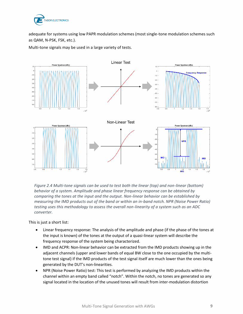
Multi-tone signals may be used in a large variety of tests.

Figure 2.4 Multi-tone signals can be used to test both the linear (top) and non-linear (bottom) behavior of a system. Amplitude and phase linear frequency response can be obtained by comparing the tones at the input and the output. Non-linear behavior can be established by measuring the IMD products out of the band or within an in-band notch. NPR (Noise Power Ratio) testing uses this methodology to assess the overall non-linearity of a system such as an ADC converter.

This is just a short list:

• Linear frequency response: The analysis of the amplitude and phase (if the phase of the tones at

the input is known) of the tones at the output of a quasi-linear system will describe the

frequency response of the system being characterized.

• IMD and ACPR: Non-linear behavior can be extracted from the IMD products showing up in the

adjacent channels (upper and lower bands of equal BW close to the one occupied by the multi-

tone test signal) if the IMD products of the test signal itself are much lower than the ones being

generated by the DUT’s non-linearities.

• NPR (Noise Power Ratio) test: This test is performed by analyzing the IMD products within the

channel within an empty band called “notch”. Within the notch, no tones are generated so any

signal located in the location of the unused tones will result from inter-modulation distortion


and noise within the channel. The NPR value, or the ratio between the power of the signal in the

notch and the power of the original tones before removal, is a factor of merit relative to the IMD

within the channel.

• I/Q Modulator imbalance characterization: Convenient complex (I/Q) multi-tone signals may be

applied to I/Q modulators, so the unwanted images caused by amplitude imbalance and

quadrature error can be established over the whole modulation bandwidth at once.

• ADC testing: The NPR measurement methodology can be applied to Analog-to-Digital Converters

to establish both the linear and non-linear responses. NPR measurements can be converted to

effective bits (ENoB) for narrow and wideband signals in a more realistic way than single-tone

tests. However, the useful dynamic range of the multi-tone signal itself must be much better (at

least 4 times, or one effective bit) than that of the ADC under test.


3 Generating Multi-tone Signals Multi-tone signals, to be useful, must be generated in a convenient and cost-effective way with

sufficient quality to address the target application. One of the important issues to consider is the

frequency band to be covered and the ratio between the central frequency and the bandwidth of the

multi-tone signal. Another important consideration is the number of carriers to be generated and the

required average power, peak power, and SFDR (Spurious Free Dynamic Range) necessary to match the

application requirements. The type of test to be performed and if it requires controll ing the relative

phase of the tones may also influence the choice of multi-tone generation architecture.

Probably, the simplest way to generate a multi-tone signal is by combining multiple CW generators, one

for each tone.


Figure 3.1 The most direct way to generate multi-tone signals is by using multiple CW generators and combining the outputs to a single signal. Absolute frequency, tone spacing, and amplitudes are easy to control this way. SFDR is as big as that of the individual CW generators. However, relative phase for the tones is not possible to control so its distribution will be like random, and PAPR will be high and it will grow with the number of tones. Other considerations are cost and size of the solution. Multi-channel analog RF/uW generators such as the Tabor Lucid LS12916R ( 16 channels up to 12 GHz in a very compact form factor), greatly reduce cost per tone and size.


All the outputs must be added together using an N-way passive combiner, so no additional distortion is

introduced into the system. One of the advantages of this arrangement is that as all the generators are

independent and a passive combiner is used, no IMD will be generated in the process and a very good

SFDR can be reached. If the generators are not locked to the same reference, frequency spacing (and

relative phase) between tones may change over time and lead to a variable spacing and PAPR. The Tabor

Lucid series of multi-channel analog RF/W generators is an example of a device especially adequate

for multi-tone generation. These generators can support up to 16 independent channels internally

locked to the same reference in a single 19” rackmount unit. Amplitude and frequency can be set

independently for each channel, so any tone arrangement can be implemented, including multi-tone

with none, one or more notches. This architecture has some drawbacks. First of all, the number of tones

will be always limited by cost or implementation issues. Combining multiple channels into a single

output using a low-IMD (passive) combiner is not free as the insertion loss grows with the number of

signals being added together. CW generators can have a very large SFDR for frequency bands close to

the tone frequency. However, harmonics can be significant, and they may show up within the band of

interest when the ratio between the central frequency and the overall multi-tone bandwidth is low.

Using this architecture should be restricted to the generation of limited BW (relative to the central

frequency), a limited number of tones (a few tens), in applications where controlling the carrier phase

distribution is not critical.

An alternative way to generate multi-tone signals is using a two-channel AWG to generate a baseband

complex (I/Q), multi-tone signal that can be supplied to an additional I/Q modulator. While amplitude,

spacing and phase of the carriers are controlled by the complex signal generated by the AWG, the

central frequency may be set independently actuating on the LO (Local Oscillator) associated to the

modulator. This strategy has two important limitations. First, the bandwidth of the multi-tone signal is

limited by either the usable bandwidth of the AWG or the modulation bandwidth of the I/Q modulator.

Second, any imbalance, differential delay or quadrature error will show up as images in the output

signal, (see figure below) either affecting the amplitude and phase accuracy of the tones (if the images

are located in the same frequencies as the valid tones), or as unwanted spurious tones (for notches or

if the images are not located at the frequency of the valid tones).


Figure 3.2 Two-channel AWGs can create I/Q signal to generate a multi-tone signal at any frequency supported by an external IQ modulator (a). However, the system must be very carefully aligned as unwanted tones can show up as images (i.e. in the notch) even when non-linearities are small due to quadrature errors, imbalance of I/Q skew. Some high-performance AWGs, such as the Tabor Proteus series, can implement numerically IQ modulation and up-conversion (b). As modulation is produced numerically (including the generation of the quadrature L.O.), there are no modulator alignment issues.


A careful calibration and alignment procedure may be necessary in order to obtain a good-enough

result. In many situations, differential linear predistortion of the I and Q components must be applied

to reduce unwanted images to the required levels. The number of tones or controlling their phase is

not a problem this time as tones are basically defined mathematically and spacing and relative phases

can be precisely and consistently set. The Tabor Proteus family of AWGs are a good example of AWGs

that can be used for this application. With up to 12 channels per desktop/benchtop unit and tens of

channels in the PXIe modular form factor, they can feed multiple external I/Q modulators

simultaneously so they can be combined to cover much higher bandwidths if necessary. The Lucid series

multi-channel analog RF generator can be used as a LO source for any external I/Q modulator.

Finally, multi-tone signals can be generated directly using a one-channel AWG if there is sufficient

analog bandwidth and sample rate to reach the maximum frequency.

Figure 3.3 AWGs can generate multi-tone signals by synthesizing the waveform mathematically and converting it to analog through their output DACs. AWGs can generate the quadrature baseband waveforms (I/Q) to feed an external quadrature modulator (a) or, if analog BW and sampling rate are sufficient, generate an IF or RF multi-tone signal directly (b). While requirements for a sampling rate may be much higher for direct generation, the usage of an external IQ modulator makes the alignment of the integrated generation system cumbersome.


AWGs can generate signals between DC and SR/2, and even beyond, if all the tones are located within

any of the Nyquist zones. AWGs provide full control of the tone characteristics (number, frequency,

phase, amplitude, notches) over an amazing bandwidth, and without any limitation regarding the

absolute and relative location of the tones. Tone spacing can be very wide and very narrow and this is

only limited by the size of the waveform memory. There are some limitations too. As all the tones are

generated by the same device, any non-linearity in the device will show up as IMD components at the

outputs. Even ideal DACs are inherently non-linear devices. Real-world DACs and wideband output

stages will add additional non-linearities. However, all these limitations can be controlled if the signals

are generated and corrected in the right way. AWGs are perfect for this as they can generate pre-

distorted signals to compensate for any linear or non-linear imperfection. The Tabor Proteus

P908x/P948x family of AWGs, with 9GSa/s sampling rate and a usable BW greater than 8GHz, is a good

example of an ideal device for multi-tone signal generation.


4 Generating Multi-tone Signal with AWGs AWGs can generate a fully defined baseband (I/Q complex signal with two channels) or an IF/RF (real

signal with just one channel) multi-tone signal from a mathematically defined waveform. Continuous

generation is possible thanks to the seamless looping capability existing in all arbitrary waveform

generators. No matter the size of the waveform memory, eventually, the waveform will have to be

looped in order to keep the signal alive as long as any test may require. Calculating the samples to be

stored in the memory is as simple as applying the following expression (see 6 Appendix A – Multi-tone

Waveform Calculation MATLAB Script, page 27 for a MATLAB script using the multi-tone calculation

methodology shown below):

W(n) = S A(i) * cos( 2 * p * (f0 + i * Df) * n /SR + f(i)), i = 0,…M-1, n = 0,…N-1 (1)

However, successful generation of a multitone signal requires meeting some conditions to make sure

that it can be looped seamlessly. In order to obtain a continuous, seamless looping, it is enough to make

sure that for all the tones, an integer number of cycles will be stored in the available waveform memory.

This can be accomplished by choosing the right sample rate, waveform length and, if necessary,

modifying the tones’ frequencies while keeping equal spacing for all of them. The best way to define

the signal generation parameters is, probably, to define the target Sample Rate. The basic Period (P) of

the multi-tone signal can be calculated from the f parameter:

P = 1 / Df (2)

The initial Time Window (TW) to be implemented in the waveform memory can be any integer multiple

of the Period P:

TW = k * P, k = 1,2,3… (3)

The number of samples to implement the TW (RL0) depends on the Sample Rate (SR):

WL0 = round(TW * SR) (4)

The rounding to an integer in the above expression results in the need to modify the Df parameter so

an integer number of periods are stored in the actual waveform length. The actual time window (TW’)

will be:

TW’ = WL0 * SR (5)

And the actual spacing (Df’) will be:

Df’ = Df * TW/TW’ (6)

All high-speed AWGs require the actual record length to be a multiple of some integer (G or Granularity).

So, the actual waveform length (WL1) will have to be modified to meet the granularity requirement. A

simple way to fulfill this requirement is by rounding the waveform length to the nearest valid integer:

WL1 = round(WL0 / G) * G (7)

The above expression results in a coarse rounding of the waveform length so the actual f after applying

(5) and (6) will be less accurate. A different way to solve the granularity problem is by repeating the

same basic waveform length as many times as required to obtain a multiple of G so the f’ calculated

in (5) will be kept. This can be calculated through the minimum common multiple (mcm) operator:


WL1’ = mcm(WL0, G) (8)

So far, just the record length and the actual f have been obtained. The other parameter that must be

adjusted is f0 so an integer multiple of cycles are stored for all the tones. One of the ways to fulfill this

requirement is choosing a reference tone (typically the first one, the last one, or the one in the middle)

and obtaining the closest frequency meeting the criteria. The reference frequency must be calculated

with the original parameters:

Fn = f0 + n * Df (9)

Any periodic signal with an integer number of cycles for a given time window must have a frequency

that must be a multiple of:

Fr = SR / WL1 (10)

The reference frequency must be rounded to the nearest multiple of that frequency:

Fn ‘ = round(Fn / Fr) * Fr (11)

Once the reference frequency has been adjusted and using the tone spacing already calculated, the

frequency of the first tone can be obtained:

F0 ‘ = Fn ‘ – n * Df’ (12)

Final frequencies for all the tones can be obtained:

Fi ‘ = F0 ‘ + i * Df’, i = 0…N-1 (13)

As the amplitude and phase for each tone does not affect the looping continuity behavior of the

resulting signal, the samples for the waveform can be calculated using expression (1) with the frequency

values listed in (13). As a rule of thumb, the longer the waveform length, the lower the frequency errors

for the tones. Selecting a high k in expression (3) and choosing the granularity handling strategy shown

in expression (8) will be better to reduce frequency error. If the resulting frequency errors are not

acceptable, f’ can be corrected by modifying the sampling rate (SR’):

SR’ = SR * TW’ / TW, so Df’ = Df (14)

In this case, f0 must be recalculated as well using expression (11).

Real-world AWGs will not generate ideal multi-tone signals, even at those corrected frequencies. They

will be affected by linear and non-linear distortions and different noise components. Linear distortions

are a consequence of the non-flat amplitude, nonlinear-phase frequency response of any arbitrary

waveform generator.


Figure 4.1 The linear distortions added by the AWG frequency response can be characterized and corrected in the first Nyquist Band (a) or the second (or higher) Nyquist band (b). This correction results in a high-quality multi-tone signal with a very accurate statistical behavior (PAPR, CCDF). It is not possible to correct the multi-tone signal simultaneously in the first and second Nyquist band without using external filters. For this reason, multi-tone signals must always fit in one of the Nyquist bands.

Overall frequency response is made of two components. One is the combined frequency responses of

the DAC, the output stage, and any cabling, component and fixturing attached to the output. This

component does not depend on the sampling rate. The second component is the zeroth-order hold

response of the DAC. Theoretically, this frequency response for amplitude takes the shape of a sinc(k*f)

with all its zeros located at the sampling frequency and its multiples while phase response is linear as it

only adds some constant delay. Multi-tone signals are an excellent method to measure the overall

amplitude/phase frequency response if a flat response analysis instrument is available, so correction

factors can be obtained through a calibration procedure. Spectrum Analyzers (SAs) usually offer a good

frequency range, a good flatness, and an excellent dynamic range. However, these instruments are not

sensitive to phase, so phase response cannot be established. Maximally flat response DSOs (Digital

Storage Oscilloscopes) are also a good alternative. These scopes have corrected amplitude and phase

response themselves, so they show an excellent flatness and phase linearity, and frequency-domain

measurements are possible through the usage of the built-in FFT function. However, they do not offer

an extremely good dynamic range. Spectrum analyzers are the best choice to analyze multi-tone signals

when only amplitude correction is required. However, DSOs should be the tool of choice if both

amplitude and phase must be corrected. Correction factors can be used to correct the results at the


output of the DUT, or they can be used to correct the multi-tone signal being generated, so the output

will reflect the actual frequency response of the DUT. Expression (1) should be extended to include

these corrections:

W(n) = S C(i) * A(i) * cos( 2 * p * (f0 + i * Df) * n /SR + f(i) + fc(i)) (15)

It is important to understand that linear corrections will typically boost the higher frequency

components, and it will modify the PAPR of the corrected signal. The most likely effect will be that the

flatness will be better, but the overall signal power will be reduced and, therefore, dynamic range will

also be reduced. Correcting multi-tone signals where differences between tones are larger than

10/15 dB may result in low-quality signals.

Non-linear behavior has also two main components. One of them is the non-linear nature of the DAC

itself, even when it is ideal as quantization is a non-linear operation. In addition to quantization, the

effects of INL (Integral Non-Linearity) and DNL (Differential Non-Linearity) will also add to the effects.

The second component is the non-linear response of the output stage and any active component

attached to the output of the generator. In order to use multi-tone signals as test signals, to check the

non-linear behavior of some DUT, the non-linearities of the signal itself must be much lower than those

expected to be measured in the DUT. External components cannot be controlled by the AWG (although

they may be corrected as it will be seen in the next section), so the internal processing blocks and

components, are going to be analyzed here. The output stage is especially important as today’s state of

the art DACs can show an excellent linearity. Some AWGs, such as the Proteus series, can alternatively

incorporate an output amplifier or a direct, unamplified connection from the DAC. Difference, in terms

of SFDR and IMD products, may be huge in favor of the second choice.

Quantization noise is one of the unwanted signal components, see Figure 4.2 a). When generating a

periodic signal, like a multi-tone signal in a seamless loop, quantization noise also repeats for each loop

so its spectrum will be made of a series of tones located at multiples of the repetition frequency. When

only one period of the multi-tone signal is stored in the waveform memory, quantization noise will show

up exactly where tones and regular IMD products are located, including notches. The solution to this

problem is setting k in expression (3) to a large number, and making sure that the different periods in

the waveform memory never repeat exactly, see Figure 4.2 b). One way to make sure this condition is

met is assigning a high-enough primer number while making sure the waveform length is not a multiple

of it. Quantization noise tones will be still there but as there will be many more of them and the overall

power stays the same, the average power for them will be lower. IMD caused by amplifiers and INL will

keep the same period of a single multi-tone period, they will show up as regular IMD products, though.

Another way to greatly reduce the effects of quantization noise is by using the AWG’s internal DUC. As

the carriers generated by the internal NCOs (Numerical Controlled Oscillators) are not synchronous with

the I/Q waveforms, the output signal does not repeat exactly in the same way at each loop of the

waveform memory and this “spreads” out quantization noise, see Figure 4.2 c).


Figure 4.2 Quantization Noise is a component of any signal generated by an AWG. In AWGs, continuous signals, such as multi-tone signals are generated by looping a self-consistent fragment stored in the waveform memory. As this segment repeats, quantization noise will also repeat, and it will show up as additional tones in the signal’s spectrum a). If the same section is calculated in such a way that several non-exactly equal segments quantization noise will repeat over a long period and more tones with a lower amplitude will show up, so the SFDR will improve b). Using an internal DUC is equivalent to applying real-time dithering and the discrete tones will disappear from the spectrum, and replace by a dense, continuous background noise, so SFDR will improve even further b).

The above distortions and noise sources are part of the ENoB (Effective Number of Bits) specification.

It tries to express the quality of some AWG (or a DAC) as that of an ideal DAC of some resolution (6

Appendix A – Multi-tone Waveform Calculation MATLAB Script, page 27). However, the impact of the

different components affecting ENoB may be very different on a multi-tone signal so this parameter by

itself it is not a good enough differentiator between products.

Signal quality in terms of IMD products and SFDR can be optimized following these guidelines:

1. Select the highest possible sampling rate as this improves flatness and spreads quantization

noise over a larger BW so its noise power density is reduced.

2. If possible, make sure that the sampling rate is selected in such a way that the image of any

harmonics of the fundamental multi-tone signal is located far from the band of interest.

3. Select a large prime number of multi-tone cycles and make sure the waveform length is not a

multiple of it.

4. Use the best possible phase distribution to obtain a good enough PAPR so the maximum overall

power is obtained while keeping the target peak power. Avoid constant distributions.

5. Use the best possible output stage if no linearity corrections are available.

6. Make sure external components such as amplifiers, mixers of modulators are up to the task.

7. Use a linear correction tool to compensate for the frequency response of the AWG and any

components or block attached to it.

8. Apply non-linear corrections if possible (see 5 Correcting Non-Linear Behavior, page 23).


5 Correcting Non-Linear Behavior SFDR is probably the most limiting factor when using a multi-tone signal for a given test. In previous

sections, the best practices to maximize this parameter have been shown and discussed. However, IMD

caused by non-linearities will always show up in the final signal. It will be visible as unwanted tones in

the adjacent channels or within the notch implemented for in-band testing. In the previous section, the

way to characterize and correct linear distortions have been discussed. The key is that AWGs can

produce pre-distorted signals that after going through the conversion chain result in an undistorted

versions of them. Can this concept be applied to non-linear behavior? The answer is yes, with some

limits. Theoretically, if the non-linear distortion mechanism was fully known and invariant, the signal

stored in the waveform memory could be non-linearly pre-distorted and generated as an undistorted

signal at the output. In this case the problem is knowing the non-linear distortion mechanism, as

different sources can show up as similar effects in the output signal. A good example is static non-

linearity and dynamic non-linearity. While static non-linearity is relatively simple to determine, dynamic

non-linearity may be extremely difficult to characterized and described mathematically and it is not

possible to pre-distort a given waveform without this detailed mathematical description.

Multi-tone signals are not any kind of signal and, fortunately, there is some characterization and

correction strategy that does not require any knowledge about the distortion generation mechanism.

This methodology is known as the Nulling-Tones technique.


Figure 5.1 The nulling tones method consists in characterizing the amplitude and phase of unwanted IMD tones and apply an interfering tone with the same amplitude and opposite phase (as seen in step 3). While measuring the amplitude accurately over a large dynamic range is quite simple, using a Spectrum Analyzer, phase cannot be established directly. Instead, two interfering tones of the same amplitude and two known phases can be applied, and the resulting amplitude measured (Step 1). From the relative amplitudes of both measurements, the unwanted tone phase can be obtained (step 2). This process must be made on all the unwanted tones simultaneously and often it is necessary to iterate the process due to the amplitude readings errors (amplitudes are measured close to the SA’s floor noise).


This method will remove unwanted IMD products, leveraging that these products are relatively small

compared to the wanted tones. For this reason, the non-linear behavior of the system being corrected

will change gently if the changes in the input waveform are small. The algorithm follows these steps:

1. Correct linear response including IQ modulator alignment, if necessary.

2. Calculate an uncorrected multi-tone signal.

3. Download the multi-tone signal and generate it.

4. Measure the amplitude of all the IMD products to be removed (adjacent channels, notch) using

a Spectrum Analyzer.

5. Add sequentially test tones in phase and quadrature of the measured amplitude to all the

frequencies to correct and measure the amplitudes.

6. From the I and Q amplitude values, the phase of the unwanted tone can be calculated.

7. Add a tone with equal amplitude and opposite phase for each unwanted tone as calculated in

step 6.

8. Go to step 3 until a number of iterations or some power level after corrections are reached.

The nulling tone will keep updating for each iteration until the required level of tone suppression is

obtained. This correction cannot be done in one step, for two reasons. One is that the amplitude

accuracy of the SA when performing high dynamic range measurements, may be limited. The other is

that as all the tones to be nulled change, the overall signal will change as well, and even if the change

is relatively small, non-linear effects may be altered. The iterative method makes sure that the changes

get smaller and smaller for each step and the nulling-tones will converge to a solution.

Using the technique described above one does not have to know anything about the nature of the tone

being nulled, so it can also be used to remove any coherent tone from any other source. Just as linear

corrections, it can be used for multi-tone signals generated in any Nyquist band. It can also compensate

for non-linearities from any external device such as amplifiers, modulators, or mixers. This capability is

extremely powerful when the application requires applying high-power signals, as it allows using limited

performance RF amplifiers, see below figure.


Figure 5.2 The actual output of a 160 MHz BW multi-tone signal at 1.1 GHz directly generated by an AWG can be seen is a). In addition to the wanted tones, there are some IMD products and background noise (most of it quantization noise). In b), the same signal after going through a nulling-tones procedure. The unwanted tones have disappeared under the background noise. In c), the multi-tone signal is generated by using an internal DUC and a complex IQ waveform at a much slower sampling rate. The background quantization noise is greatly reduced. Finally, in d), the same signal is generated using half of the DAC range (6dB attenuation can be observed). Notice that the level of the IMD products are greatly reduced at the expense of a lower amplitude and SNR. Applying the nulling-tones procedure to the signal in c), the same or better level of spurious IMD products could be reached while preserving the precious dynamic range.


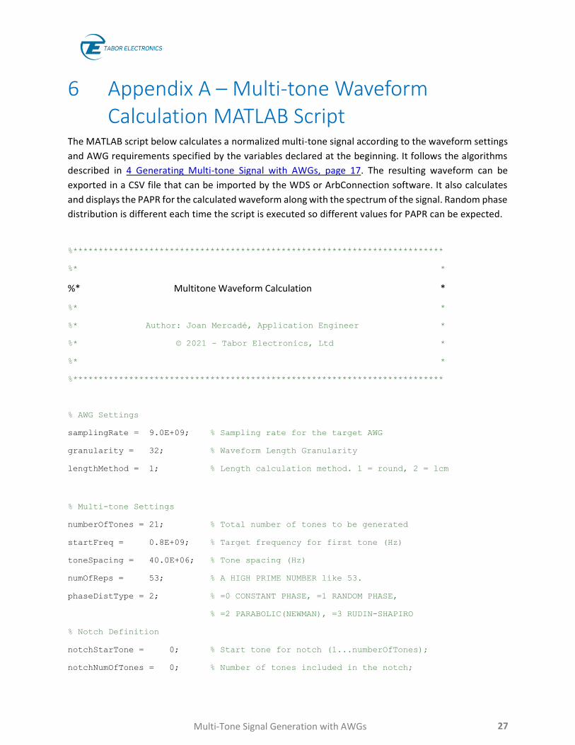
6 Appendix A – Multi-tone Waveform Calculation MATLAB Script

The MATLAB script below calculates a normalized multi-tone signal according to the waveform settings

and AWG requirements specified by the variables declared at the beginning. It follows the algorithms

described in 4 Generating Multi-tone Signal with AWGs, page 17. The resulting waveform can be

exported in a CSV file that can be imported by the WDS or ArbConnection software. It also calculates

and displays the PAPR for the calculated waveform along with the spectrum of the signal. Random phase

distribution is different each time the script is executed so different values for PAPR can be expected.

%*************************************************************************

%* *

%* Multitone Waveform Calculation *

%* *

%* Author: Joan Mercadé, Application Engineer *

%* © 2021 - Tabor Electronics, Ltd *

%* *

%*************************************************************************

% AWG Settings

samplingRate = 9.0E+09; % Sampling rate for the target AWG

granularity = 32; % Waveform Length Granularity

lengthMethod = 1; % Length calculation method. 1 = round, 2 = lcm

% Multi-tone Settings

numberOfTones = 21; % Total number of tones to be generated

startFreq = 0.8E+09; % Target frequency for first tone (Hz)

toneSpacing = 40.0E+06; % Tone spacing (Hz)

numOfReps = 53; % A HIGH PRIME NUMBER like 53.

phaseDistType = 2; % =0 CONSTANT PHASE, =1 RANDOM PHASE,

% =2 PARABOLIC(NEWMAN), =3 RUDIN-SHAPIRO

% Notch Definition

notchStarTone = 0; % Start tone for notch (1...numberOfTones);

notchNumOfTones = 0; % Number of tones included in the notch;


% Export CSV File Creation

saveFile = false; % Save file

fName = "RefToneFile.csv"; % File name

% Record Length And Parameter Calculation

% Base Freq Resolution

repOfReps = 1;

freqRes = toneSpacing / numOfReps;

% Integer waveform length closest to the required resolution

wfmLength = round(samplingRate / freqRes);

% final wfmLength calculation to meet the granularity requirement

if lengthMethod == 2

repOfReps = lcm(wfmLength, granularity) / wfmLength;

wfmLength = lcm(wfmLength, granularity);

else

wfmLength = granularity * round (wfmLength / granularity);

end

% Actual freq resolution depends on the final waveform length

freqRes = samplingRate / wfmLength;

% Actual toneSpacing depends on the final freqRes

toneSpacing = freqRes * numOfReps * repOfReps;

% Start and final frequencies are calculated

startFreq = round(startFreq / freqRes) * freqRes;

finalFreq = startFreq + (numberOfTones - 1) * toneSpacing;

% Waveform Creation

% Time values are calculated for each sample

xValues = 0 : (wfmLength - 1);

xValues = xValues / samplingRate;

% Amplitude is flat by default (all ones)

amplTable = ones(1, numberOfTones);


% Actual tone frequencies are calculated for each tone

freqTable = startFreq : toneSpacing : finalFreq;

% Phase initialized to tones

phaseTable = zeros(1, numberOfTones);

% Notch Insertion

if notchStarTone > 0 && notchNumOfTones > 0

amplTable(notchStarTone : notchStarTone + notchNumOfTones - 1) = 0.0;

end

% Phase Set Up

% Random Phase

if phaseDistType == 1

phaseTable = 2.0 * pi .* (rand(1, numberOfTones) - 0.5);

end

% Parabolic Phase (NEWMAN)


phaseTable = 1:numberOfTones;

phaseTable = 1.0 - phaseTable .* phaseTable;

phaseTable = -(pi / numberOfTones) .* phaseTable;

phaseTable = wrapToPi(phaseTable);

end

% Rudin Sequence (near optimal for 2^N tones)


numOfSteps = int16(round(log(numberOfTones) / log(2)));

if 2^numOfSteps < numberOfTones

numOfSteps = numOfSteps + 1;

end

numOfSteps = numOfSteps - 1;

temPhase(1:2) = 1;

for n = 1:numOfSteps


m = int16(length(temPhase) / 2);

temPhase = [temPhase, temPhase(1 : m), -temPhase(m + 1 : 2 * m)];

end

phaseTable = -0.5 * pi .* (temPhase(1 : numberOfTones) - 1);

end

% Multi-tone Waveform Calculation (I/Q)

multiToneWfm = zeros(1, wfmLength);

freqTable = 2.0 * pi * freqTable;

for i = 1:numberOfTones

multiToneWfm = multiToneWfm + ...

amplTable(i) .* cos(freqTable(i) .* xValues + phaseTable(i));

end

% Normalization to the -1.0/+1.0 Range

maxValue = max(abs(multiToneWfm));

multiToneWfm = multiToneWfm ./ maxValue;

% Calculation of PAPR (Crest Factor)

papr = 1.0 / std(multiToneWfm);

papr = 20.0 * log10 (papr) - 3.0;

% File Creation

if saveFile

csvwrite(fName, multiToneWfm');

end

% Plot Spectrum

pSpec = pspectrum(flattopwin(1, wfmLength) .* multiToneWfm);


pSpec = 10.0 * log10(pSpec);

pSpec = pSpec-max(pSpec);

xFreq = 0:(length(pSpec)-1);

xFreq = xFreq / (2 * length(pSpec));

xFreq = xFreq *samplingRate;

plot(xFreq, pSpec);

axis([-inf +inf -80 20]);

title(strcat('Power Spectrum (dBc), PAPR = ', num2str(papr), 'dB'));


Document Revision History

Table Document Revision History

Revision Date Description Author

1.0 07-Apr-2021 • Original release. Joan Mercade

Acronyms & Abbreviations

Table Acronyms & Abbreviations

Acronym Description

µs or us Microseconds

ACPR Adjacent Channel Power Ratio

ADC Analog to Digital Converter

AM Amplitude Modulation

ASIC Application-Specific Integrated Circuit

ATE Automatic Test Equipment

AWG Arbitrary Waveform Generators

AWT Arbitrary Waveform Transceiver

BNC Bayonet Neill–Concelm (coax connector)

BW Bandwidth

CCDF Complementary Cumulative Distribution Function

CW Continuous Wave

CW Carrier Wave

DAC Digital to Analog Converter

dBc dB/carrier. The power ratio of a signal to a carrier signal, expressed in decibels

dBm Decibel-Milliwatts. E.g., 0 dBm equals 1.0 mW.

DDC Digital Down-Converter

DHCP Dynamic Host Configuration Protocol

DNL Differential Non-Linearity


Acronym Description

DSO Digital Storage Oscilloscope

DUC Digital Up-Converter

DUT Device Under Test

ENoB Effective Number of Bits

ESD Electrostatic Discharge

EVM Error Vector Magnitude

FPGA Field-Programmable Gate Arrays

FW Firmware

GHz Gigahertz

GPIB General Purpose Interface Bus

GS/s Giga Samples per Second

GUI Graphical User Interface

HP Horizontal Pitch (PXIe module horizontal width, 1 HP = 5.08mm)

Hz Hertz

IF Intermediate Frequency

IMD Intermodulation Distortion

INL Integral Non-Linearity

I/O Input / Output

IP Internet Protocol

IQ In-phase Quadrature

IVI Interchangeable Virtual Instrument

JSON JavaScript Object Notation

kHz Kilohertz

LCD Liquid Crystal Display

LO Local Oscillator

MAC Media Access Control (address)

MDR Mini D Ribbon (connector)

MHz Megahertz


Acronym Description

ms Milliseconds

NCO Numerically Controlled Oscillator

ns Nanoseconds

OFDM Orthogonal Frequency-Division Multiplexing

PAM Pulse-amplitude Modulation

PAPR Peak-to-Average Power Ratio

PC Personal Computer

PCAP Projected Capacitive Touch Panel

PCB Printed Circuit Board

PCI Peripheral Component Interconnect

PXI PCI eXtension for Instrumentation

PXIe PCI Express eXtension for Instrumentation

QC Quantum Computing

Qubits Quantum bits

R&D Research & Development

RF Radio Frequency

RT-DSO Real-Time Digital Oscilloscope

s Seconds

SA Spectrum Analyzer

SCPI Standard Commands for Programmable Instruments

SFDR Spurious Free Dynamic Range

SFP Software Front Panel

SINAD Signal-to-Noise-And-Distortion Ratio

SMA Subminiature version A connector

SMP Subminiature Push-on connector

SNR Signal-to-Noise Ratio

SPI Serial Peripheral Interface

SQNR Signal to Quantization Noise Signal


Acronym Description

SRAM Static Random-Access Memory

TFT Thin Film Transistor

T&M Test and Measurement

TPS Test Program Sets

UART Universal Asynchronous Receiver-Transmitter

USB Universal Serial Bus

VCP Virtual COM Port

Vdc Volts, Direct Current

V p-p Volts, Peak-to-Peak

VSA Vector Signal Analyzer

VSG Vector Signal Generator

WDS Wave Design Studio


Resources & Contact

For more information on microwave signal generation challenges and solutions, review the following

resources:

⧫ White Paper: Multi-Nyquist Zones Operation-Solution Note

⧫ Solution Brief: Envelope Tracking – Solution Note

⧫ Datasheet Proteus - Arbitrary Waveform Generator / Transceiver: Module Desktop Benchtop

⧫ Datasheet Proteus - RF Arbitrary Waveform Generator / Transceiver: Module Desktop Benchtop

⧫ Online Webinar: Experiment design considerations for real-time, closed-loop pulse streaming

Stay Up To Date

⧫ www.taborelec.com

⧫ LinkedIn page

⧫ YouTube channel

Corporate Headquarters

Address: 9 Hata’asia St., 3688809 Nesher, Israel

Phone: (972) 4 821 3393

Fax: (972) 4 821 3388

For Information

Email: [email protected]

For Service & Support


US Sales & Support (Astronics)

Address: 4 Goodyear Irvine, CA 92618

Phone: (800) 722 2528

Fax: (949) 859 7139

For Information


For Service & Support


All rights reserved to Tabor Electronics LTD. The contents of this document are provided by Tabor

Electronics, 'as is'. Tabor makes no representations nor warranties with respect to the accuracy or

completeness of the contents of this publication and reserves the right to make changes to the

specification at any time without notice.

https://www.taborelec.com/multi-nyquist-zones-operation-solution-note

https://www.taborelec.com/Envelope-Tracking-Solution-Note

https://www.taborelec.com/GenericHendler/GetFile.ashx?D=0&DG=3843






https://www.taborelec.com/Experiment-design-considerations-for-real-time-closed-loop-pulse-streaming

http://www.taborelec.com/

http://www.linkedin.com/company/tabor-electronics

https://www.youtube.com/user/Taborelectronicsltd

mailto:[email protected]




Multi-Tone Signal Generation with AWGs

Documents

Transcript of Multi-Tone Signal Generation with AWGs