Multi-Scale Orderless Pooling of Deep Convolutional...

Multi-Scale Orderless Pooling ofDeep Convolutional Activation Features

Yunchao Gong1, Liwei Wang2, Ruiqi Guo2, and Svetlana Lazebnik2

1University of North Carolina at Chapel [email protected]

2University of Illinois at Urbana-Champaign{lwang97,guo29,slazebni}@illinois.edu

Abstract. Deep convolutional neural networks (CNN) have shown theirpromise as a universal representation for recognition. However, globalCNN activations lack geometric invariance, which limits their robustnessfor classification and matching of highly variable scenes. To improve theinvariance of CNN activations without degrading their discriminativepower, this paper presents a simple but effective scheme called multi-scale orderless pooling (MOP-CNN). This scheme extracts CNN activa-tions for local patches at multiple scale levels, performs orderless VLADpooling of these activations at each level separately, and concatenates theresult. The resulting MOP-CNN representation can be used as a genericfeature for either supervised or unsupervised recognition tasks, from im-age classification to instance-level retrieval; it consistently outperformsglobal CNN activations without requiring any joint training of predictionlayers for a particular target dataset. In absolute terms, it achieves state-of-the-art results on the challenging SUN397 and MIT Indoor Scenes clas-sification datasets, and competitive results on ILSVRC2012/2013 classi-fication and INRIA Holidays retrieval datasets.

1 Introduction

Recently, deep convolutional neural networks (CNN) [1] have demonstratedbreakthrough accuracies for image classification [2]. This has spurred a flurryof activity on further improving CNN architectures and training algorithms[3,4,5,6,7], as well as on using CNN features as a universal representation forrecognition. A number of recent works [8,9,10,11,12] show that CNN featurestrained on sufficiently large and diverse datasets such as ImageNet [13] can besuccessfully transferred to other visual recognition tasks, e.g., scene classifica-tion and object localization, with a only limited amount of task-specific trainingdata. Our work also relies on reusing CNN activations as off-the-shelf features forwhole-image tasks like scene classification and retrieval. But, instead of simplycomputing the CNN activation vector over the entire image, we ask whether wecan get improved performance by combining activations extracted at multiplelocal image windows. Inspired by previous work on spatial and feature spacepooling of local descriptors [14,15,16], we propose a novel and simple pooling

2 Y. Gong et al.

scheme that significantly outperforms global CNN activations for both super-vised tasks like image classification and unsupervised tasks like retrieval, evenwithout any fine-tuning on the target datasets.

Image representation has been a driving motivation for research in computervision for many years. For much of the past decade, orderless bag-of-features(BoF) methods [15,17,18,19,20] were considered to be the state of the art. Es-pecially when built on top of locally invariant features like SIFT [21], BoF canbe, to some extent, robust to image scaling, translation, occlusion, and so on.However, they do not encode global spatial information, motivating the incorpo-ration of loose spatial information in the BoF vectors through spatial pyramidmatching (SPM) [14]. Deep CNN, as exemplified by the system of Krizhevskyet al. [2], is a completely different architecture. Raw image pixels are first sentthrough five convolutional layers, each of which filters the feature maps and thenmax-pools the output within local neighborhoods. At this point, the represen-tation still preserves a great deal of global spatial information. For example,as shown by Zeiler and Fergus [22], the activations from the fifth max-poolinglayer can be reconstructed to form an image that looks similar to the originalone. Though max-pooling within each feature map helps to improve invarianceto small-scale deformations [23], invariance to larger-scale, more global defor-mations might be undermined by the preserved spatial information. After thefiltering and max-pooling layers follow several fully connected layers, finally pro-ducing an activation of 4096 dimensions. While it becomes more difficult toreason about the invariance properties of the output of the fully connected lay-ers, we will present an empirical analysis in Section 3 indicating that the finalCNN representation is still fairly sensitive to global translation, rotation, andscaling. Even if one does not care about this lack of invariance for its own sake,we show that it directly translates into a loss of accuracy for classification tasks.

Intuitively, bags of features and deep CNN activations lie towards oppositeends of the “orderless” to “globally ordered” spectrum for visual representations.SPM [14] is based on realizing that BoF has insufficient spatial information formany recognition tasks and adding just enough such information. Inspired bythis, we observe that CNN activations preserve too much spatial information,and study the question of whether we can build a more orderless representationon top of CNN activations to improve recognition performance. We present asimple but effective framework for doing this, which we refer to as multi-scaleorderless pooling (MOP-CNN). The idea is summarized in Figure 1. Briefly, webegin by extracting deep activation features from local patches at multiple scales.Our coarsest scale is the whole image, so global spatial layout is still preserved,and our finer scales allow us to capture more local, fine-grained details of theimage. Then we aggregate local patch responses at the finer scales via VLADencoding [16]. The orderless nature of VLAD helps to build a more invariantrepresentation. Finally, we concatenatenate the original global deep activationswith the VLAD features for the finer scales to form our new image representation.

Section 2 will introduce our multi-scale orderless pooling approach. Section3 will present a small-scale study suggesting that CNN activations extracted

Multi-scale Orderless Pooling of Deep Convolutional Activation Features 3

(a) level1: global activation (b) level2: pooled features (c) level3: pooled features

…

…

4096-D activations

…

…

… …

4096-D activations4096-D activations

Kmeans + VLAD pooling Kmeans + VLAD pooling

Fig. 1. Overview of multi-scale orderless pooling for CNN activations (MOP-CNN).Our proposed feature is a concatenation of the feature vectors from three levels: (a)Level 1, corresponding to the 4096-dimensional CNN activation for the entire 256×256image; (b) Level 2, formed by extracting activations from 128×128 patches and VLADpooling them with a codebook of 100 centers; (c) Level 3, formed in the same way aslevel 2 but with 64× 64 patches.

at sub-image windows can provide more robust and discriminative informationthan whole-image activations, and confirming that MOP-CNN is more robustin the presence of geometric deformations than global CNN. Next, Section 4will report comprehensive experiments results for classification on three imagedatasets (SUN397, MIT Indoor Scenes, and ILSVRC2012/2013) and retrievalon the Holidays dataset. A sizable boost in performance across these popularbenchmarks confirms the promise of our method. Section 5 will conclude with adiscussion of future work directions.

2 The Proposed Method

Inspired by SPM [14], which extracts local patches at a single scale but thenpools them over regions of increasing scale, ending with the whole image, wepropose a kind of “reverse SPM” idea, where we extract patches at multiplescales, starting with the whole image, and then pool each scale without regardto spatial information. The basic idea is illustrated in Figure 1.

Our representation has three scale levels, corresponding to CNN activationsof the global 256 × 256 image and 128 × 128 and 64 × 64 patches, respectively.To extract these activations, we use the Caffe CPU implementation [24] pre-trained on ImageNet [13]. Given an input image or a patch, we resample itto 256 × 256 pixels, subtract the mean of the pixel values, and feed the patchthrough the network. Then we take the 4096-dimensional output of the seventh(fully connected) layer, after the rectified linear unit (ReLU) transformation, sothat all the values are non-negative (we have also tested the activations beforeReLU and found worse performance).

4 Y. Gong et al.

For the first level, we simply take the 4096-dimensional CNN activation forthe whole 256 × 256 image. For the remaining two levels, we extract activationsfor all 128 × 128 and 64 × 64 patches sampled with a stride of 32 pixels. Next,we need to pool the activations of these multiple patches to summarize thesecond and third levels by single feature vectors of reasonable dimensionality.For this, we adopt Vectors of Locally Aggregated Descriptors (VLAD) [16,25],which are a simplified version of Fisher Vectors (FV) [15]. At each level, weextract the 4096-dimensional activations for respective patches and, to makecomputation more efficient, use PCA to reduce them to 500 dimensions. Wealso learn a separate k-means codebook for each level with k = 100 centers.Given a collection of patches from an input image and a codebook of centersci, i = 1, . . . , k, the VLAD descriptor (soft assignment version from [25]) isconstructed by assigning each patch pj to its r nearest cluster centers rNN(pj)and aggregating the residuals of the patches minus the center:

x =

∑j: c1∈rNN(pj)

wj1(pj − c1), . . . ,∑

j: ck∈rNN(pj)

wjk(pj − ck)

,

where wjk is the Gaussian kernel similarity between pj and ck. For each patch,we additionally normalize its weights to its nearest r centers to have sum one. Forthe results reported in the paper, we use r = 51 and kernel standard deviationof 10. Following [16], we power- and L2-normalize the pooled vectors. However,the resulting vectors still have quite high dimensionality: given 500-dimensionalpatch activations pj (after PCA) and 100 k-means centers, we end up with50,000 dimensions. This is too high for many large-scale applications, so wefurther perform PCA on the pooled vectors and reduce them to 4096 dimensions.Note that applying PCA after the two stages (local patch activation and globalpooled vector) is a standard practice in previous works [26,27]. Finally, giventhe original 4096-dimensional feature vector from level one and the two 4096-dimensional pooled PCA-reduced vectors from levels two and three, we rescalethem to unit norm and concatenate them to form our final image representation.

3 Analysis of Invariance

We first examine the invariance properties of global CNN activations vs. MOP-CNN. As part of their paper on visualizing deep features, Zeiler and Fergus [22]analyze the transformation invariance of their model on five individual imagesby displaying the distance between the feature vectors of the original and trans-formed images, as well as the change in the probability of the correct label forthe transformed version of the image (Figure 5 of [22]). These plots show very

1 In the camera-ready version of the paper, we incorrectly reported using r = 1, whichis equivalent to the hard assignment VLAD in [16]. However, we have experimentedwith different r and their accuracy on our datasets is within 1% of each other.


original scaling ratio=10/9

v-translation = -40

horizontal flipping rotation degree 20=-

scaling ratio=10/8 scaling ratio=10/7 scaling ratio=10/6 scaling ratio=10/5 scaling ratio=10/4

vertical flipping rotation degree 10=- rotation degree 5=- rotation degree 5= rotation degree 10= rotation degree 20=

v-translation = -20 v-translation = 20 v-translation = 40 h-translation = 40h-translation = 20h-translation = -20h-translation = -40

Fig. 2. Illustration of image transformations considered in our invariance study. Forscaling by a factor of ρ, we take crops around the image center of (1/ρ) times originalsize. For translation, we take crops of 0.7 times the original size and translate them byup to 40 pixels in either direction horizontally or vertically (the translation amount isrelative to the normalized image size of 256 × 256). For rotation, we take crops fromthe middle of the image (so as to avoid corner artifacts) and rotate them from -20 to 20degrees about the center. The corresponding scaling ratio, translation distance (pixels)and rotation degrees are listed below each instance.

different patterns for different images, making it difficult to draw general conclu-sions. We would like to conduct a more comprehensive analysis with an emphasison prediction accuracy for entire categories, not just individual images. To thisend, we train one-vs-all linear SVMs on the original training images for all 397categories from the SUN dataset [28] using both global 4096-dimensional CNNactivations and our proposed MOP-CNN features. At test time, we consider fourpossible transformations: translation, scaling, flipping and rotation (see Figure2 for illustration and detailed explanation of transformation parameters). Weapply a given transformation to all the test images, extract features from thetransformed images, and perform 397-way classification using the trained SVMs.Figure 3 shows classification accuracies as a function of transformation type andparameters for four randomly selected classes: arrival gate, florist shop, volleyballcourt, and ice skating. In the case of CNN features, for almost all transforma-tions, as the degree of transformation becomes more extreme, the classificationaccuracies keep dropping for all classes. The only exception is horizontal flipping,which does not seem to affect the classification accuracy. This may be due to thefact that the Caffe implementation adds horizontal flips of all training imagesto the training set (on the other hand, the Caffe training protocol also involvestaking random crops of training images, yet this does not seem sufficient forbuilding in invariance to such transformations, as our results indicate). By con-trast with global CNN, our MOP-CNN features are more robust to the degreeof translation, rotation, and scaling, and their absolute classification accuraciesare consistently higher as well.

Figure 4 further illustrates the lack of robustness of global CNN activationsby showing the predictions for a few ILSVRC2012/2013 images based on dif-ferent image sub-windows. Even for sub-windows that are small translations ofeach other, the predicted labels can be drastically different. For example, in (f),

6 Y. Gong et al.

original 10/9 10/8 10/7 10/6 10/5 10/40

0.2

0.4

0.6

0.8

1

CNN: scaling (ratio)

Cla

ssifi

catio

n A

ccur

acy

−40 −20 original 20 400

0.2

0.4

0.6

0.8

1

CNN: vertical translation (pixels)

Cla

ssifi

catio

n A

ccur

acy

−40 −20 original 20 400

0.2

0.4

0.6

0.8

1

CNN: horizontal translation (pixels)

Cla

ssifi

catio

n A

ccur

acy

original 10/9 10/8 10/7 10/6 10/5 10/40

0.2

0.4

0.6

0.8

1

MOP−CNN: scaling (ratio)

Cla

ssifi

catio

n A

ccur

acy

(a) scaling

−40 −20 original 20 400

0.2

0.4

0.6

0.8

1

MOP−CNN: vertical translation (pixels)

Cla

ssifi

catio

n A

ccur

acy

(b) v-translation

−40 −20 original 20 400

0.2

0.4

0.6

0.8

1

MOP−CNN: horizontal translation (pixels)

Cla

ssifi

catio

n A

ccur

acy

(c) h-translation

original vertical horizontal0

0.2

0.4

0.6

0.8

1

CNN: flipping

Cla

ssifi

catio

n A

ccur

acy

−20 −10 −5 original 5 10 200

0.2

0.4

0.6

0.8

1

CNN: rotation (degrees)

Cla

ssifi

catio

n A

ccur

acy

original vertical horizontal0

0.2

0.4

0.6

0.8

1

MOP−CNN: flipping

Cla

ssifi

catio

n A

ccur

acy

(d) flipping

−20 −10 −5 original 5 10 200

0.2

0.4

0.6

0.8

1

MOP−CNN: rotation (degrees)

Cla

ssifi

catio

n A

ccur

acy

(e) rotation

Fig. 3. Accuracies for 397-way classification on four classes from the SUN dataset as afunction of different transformations of the test images. For each transformation type(a-e), the upper (resp. lower) plot shows the classification accuracy using the globalCNN representation (resp. MOP-CNN).

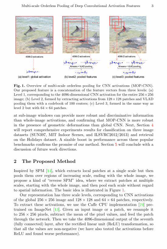
the red rectangle is correctly labeled “alp,” while the overlapping rectangle is in-correctly labeled “garfish.” But, while picking the wrong window can give a badprediction, picking the “right” one can give a good prediction: in (d), the wholeimage is wrongly labeled, but one of its sub-windows can get the correct label –“schooner.” This immediately suggests a sliding window protocol at test time:given a test image, extract windows at multiple scales and locations, computetheir CNN activations and prediction scores, and look for the window that givesthe maximum score for a given class. Figure 5 illustrates such a “scene detection”approach [29,28] on a few SUN images. In fact, it is already common for CNNimplementations to sample multiple windows at test time: the systems of [2,8,24]can take five sub-image windows corresponding to the center and four corners,together with their flipped versions, and average the prediction scores over theseten windows. As will be shown in Table 4, for Caffe, this “center+corner+flip”


alp

shovel

ski

(a) skibighorn sheep

wood rabbit

bighorn sheep

(b) bighorn sheep

water jug

loafer

hand blower

(c) pitcher

schooner

pirate

catamaran

(d) schooner

damselfly

jay

bee eater

(e) bee eater

garfish

alp

alp

(f) alpFig. 4. Classification of CNN activations of local patches in an image. The groundtruth labels are listed below each image. Labels predicted by whole-image CNN arelisted in the bottom right corner.

Fig. 5. Highest-response windows (in red) for (a) basilica, (b) control tower, (c) board-walk, and (d) tower. For each test image resampled to 256×256, we search over windowswith widths 224, 192, 160, and 128 and a stride of 16 pixels and display the windowthat gives the highest prediction score for the ground truth category. The detectedwindows contain similar structures: in (a), (b) and (d), the top parts of towers havebeen selected; in (c), the windows are all centered on the narrow walkway.

strategy gets 56.30% classification accuracy on ILSVRC2012/2013 vs. 54.34%for simply classifying global image windows. An even more recent system, Over-Feat [12], incorporates a more comprehensive multi-scale voting scheme for clas-sification, where efficient computations are used to extract class-level activationsat a denser sampling of locations and scales, and the average or maximum ofthese activations is taken to produce the final classification results. With thisscheme, OverFeat can achieve as high as 64.26% accuracy on ILSVRC2012/2013,albeit starting from a better baseline CNN with 60.72% accuracy.

While the above window sampling schemes do improve the robustness of pre-diction over single global CNN activations, they all combine activations (classifier

8 Y. Gong et al.

Table 1. A summary of baselines and their relationship to the MOP-CNN method.

pooling method / scale multi-scale concatenation

Average pooling Avg (multi-scale) Avg (concatenation)Max pooling Max (multi-scale) Max (concatenation)

VLAD pooling VLAD (multi-scale) MOP-CNN

responses) from the final prediction layer, which means that they can only beused following training (or fine-tuning) for a particular prediction task, and donot naturally produce feature vectors for other datasets or tasks. By contrast,MOP-CNN combines activations of the last fully connected layer, so it is a moregeneric representation that can even work for tasks like image retrieval, whichmay be done in an unsupervised fashion and for which labeled training data maynot be available.

4 Large-Scale Evaluation

4.1 Baselines

To validate MOP-CNN, we need to demonstrate that a simpler patch samplingand pooling scheme cannot achieve the same performance. As simpler alterna-tives to VLAD pooling, we consider average pooling, which involves computingthe mean of the 4096-dimensional activations at each scale level, and maximumpooling, which involves computing their element-wise maximum. We did notconsider standard BoF pooling because it has been demonstrated to be less accu-rate than VLAD [16]; to get competitive performance, we would need a codebooksize much larger than 100, which would make the quantization step prohibitivelyexpensive. As additional baselines, we need to examine alternative strategies withregards to pooling across scale levels. The multi-scale strategy corresponds totaking the union of all the patches from an image, regardless of scale, and pool-ing them together. The concatenation strategy refers to pooling patches fromthree levels separately and then concatenating the result. Finally, we separatelyexamine the performance of individual scale levels as well as concatenations ofjust pairs of them. In particular, level1 is simply the 4096-dimensional globaldescriptor of the entire image, which was suggested in [8] as a generic imagedescriptor. These baselines and their relationship to our full MOP-CNN schemeare summarized in Table 1.

4.2 Datasets

We test our approach on four well-known benchmark datasets:

SUN397 [28] is the largest dataset to date for scene recognition. It contains397 scene categories and each has at least 100 images. The evaluation protocolinvolves training and testing on ten different splits and reporting the averageclassification accuracy. The splits are fixed and publicly available from [28]; eachhas 50 training and 50 test images.


MIT Indoor [30] contains 67 categories. While outdoor scenes, which comprisemore than half of SUN (220 out of 397), can often be characterized by globalscene statistics, indoor scenes tend to be much more variable in terms of compo-sition and better characterized by the objects they contain. This makes the MITIndoor dataset an interesting test case for our representation, which is designedto focus more on appearance of sub-image windows and have more invariance toglobal transformations. The standard training/test split for the Indoor datasetconsists of 80 training and 20 test images per class.

ILSVRC2012/2013 [31,32], or ImageNet Large-Scale Visual Recognition Chal-lenge, is the most prominent benchmark for comparing large-scale image classifi-cation methods and is the dataset on which the Caffe representation we use [24]is pre-trained. ILSVRC differs from the previous two datasets in that most of itscategories focus on objects, not scenes, and the objects tend to be highly salientand centered in images. It contains 1000 classes corresponding to leaf nodes inImageNet. Each class has more than 1000 unique training images, and there isa separate validation set with 50,000 images. The 2012 and 2013 versions of theILSVRC competition have the same training and validation data. Classificationaccuracy on the validation set is used to evaluate different methods.

INRIA Holidays [33] is a standard benchmark for image retrieval. It contains1491 images corresponding to 500 image instances. Each instance has 2-3 imagesdescribing the same object or location. A set of 500 images are used as queries,and the rest are used as the database. Mean average precision (mAP) is theevaluation metric.

4.3 Image Classification Results

In all of the following experiments, we train classifiers using the linear SVMimplementation from the INRIA JSGD package [34]. We fix the regularizationparameter to 10−5 and the learning rate to 0.2, and train for 100 epochs.

Table 2 reports our results on the SUN397 dataset. From the results for base-line pooling methods in (a), we can see that VLAD works better than averageand max pooling and that pooling scale levels separately works better than pool-ing them together (which is not altogether surprising, since the latter strategyraises the feature dimensionality by a factor of three). From (b), we can seethat concatenating all three scale levels gives a significant improvement over anysubset. For reference, Part (c) of Table 2 gives published state-of-the-art resultsfrom the literature. Xiao et al. [28], who have collected the SUN dataset, havealso published a baseline accuracy of 38% using a combination of standard fea-tures like GIST, color histograms, and BoF. This baseline is slightly exceeded bythe level1 method, i.e., global 4096-dimensional Caffe activations pre-trained onImageNet. The Caffe accuracy of 39.57% is also comparable to the 40.94% withan analogous setup for DeCAF [8].2 However, these numbers are still worse than

2 DeCAF is an earlier implementation from the same research group and Caffe is its“little brother.” The two implementations are similar, but Caffe is faster, includessupport for both CPU and GPU, and is easier to modify.

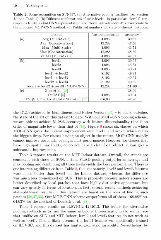
10 Y. Gong et al.

Table 2. Scene recognition on SUN397. (a) Alternative pooling baselines (see Section4.1 and Table 1); (b) Different combinations of scale levels – in particular, “level1” cor-responds to the global CNN representation and “level1+level2+level3” corresponds tothe proposed MOP-CNN method. (c) Published numbers for state-of-the-art methods.

method feature dimension accuracy

(a) Avg (Multi-Scale) 4,096 39.62Avg (Concatenation) 12,288 47.50

Max (Multi-Scale) 4,096 43.51Max (Concatenation) 12,288 48.50VLAD (Multi-Scale) 4,096 47.32

(b) level1 4,096 39.57level2 4,096 45.34level3 4,096 40.21

level1 + level2 8,192 49.91level1 + level3 8,192 49.52level2 + level3 8,192 49.66

level1 + level2 + level3 (MOP-CNN) 12,288 51.98

(c) Xiao et al. [28] – 38.00DeCAF [8] 4,096 40.94

FV (SIFT + Local Color Statistic) [35] 256,000 47.20

the 47.2% achieved by high-dimensional Fisher Vectors [35] – to our knowledge,the state of the art on this dataset to date. With our MOP-CNN pooling scheme,we are able to achieve 51.98% accuracy with feature dimensionality that is anorder of magnitude lower than that of [35]. Figure 6 shows six classes on whichMOP-CNN gives the biggest improvement over level1, and six on which it hasthe biggest drop. For classes having an object in the center, MOP-CNN usuallycannot improve too much, or might hurt performance. However, for classes thathave high spatial variability, or do not have a clear focal object, it can give asubstantial improvement.

Table 3 reports results on the MIT Indoor dataset. Overall, the trends areconsistent with those on SUN, in that VLAD pooling outperforms average andmax pooling and combining all three levels yields the best performance. There isone interesting difference from Table 2, though: namely, level2 and level3 featureswork much better than level1 on the Indoor dataset, whereas the differencewas much less pronounced on SUN. This is probably because indoor scenes arebetter described by local patches that have highly distinctive appearance butcan vary greatly in terms of location. In fact, several recent methods achievingstate-of-the-art results on this dataset are based on the idea of finding suchpatches [38,37,36]. Our MOP-CNN scheme outperforms all of them – 68.88% vs.64.03% for the method of Doersch et al. [38].

Table 4 reports results on ILSVRC2012/2013. The trends for alternativepooling methods in (a) are the same as before. Interestingly, in (b) we can seethat, unlike on SUN and MIT Indoor, level2 and level3 features do not work aswell as level1. This is likely because the level1 feature was specifically trainedon ILSVRC, and this dataset has limited geometric variability. Nevertheless, by


Playroom (+48%) Cottage Garden (+50%) Florist shop (+56%)

Poolroom (-30%) Utility room (-26%) Shed (-22%)

football stadium (+46%) Van interior (+46%) Ice Skating Rink (+48%)

Volleyball court (-18%) Industrial area (-18%) Arrival gate (-18%)

Fig. 6. SUN classes on which MOP-CNN gives the biggest decrease over the level1global features (top), and classes on which it gives the biggest increase (bottom).

combining the three levels, we still get a significant improvement. Note that di-rectly running the full pre-trained Caffe network on the global features from thevalidation set gives 54.34% accuracy (part (c) of Table 4, first line), which ishigher than our level1 accuracy of 51.46%. The only difference between thesetwo setups, “Caffe (Global)” and “level1,” are the parameters of the last clas-sifier layer – i.e., softmax and SVM, respectively. For Caffe, the softmax layeris jointly trained with all the previous network layers using multiple randomwindows cropped from training images, while our SVMs are trained separatelyusing only the global image features. Nevertheless, the accuracy of our finalMOP-CNN representation, at 57.93%, is higher than that of the full pre-trainedCaffe CNN tested either on the global features (“Global”) or on ten sub-windows(“Center+Corner+Flip”).

It is important to note that in absolute terms, we do not achieve state-of-the-art results on ILSVRC. For the 2012 version of the contest, the highest resultswere achieved by Krizhevsky et al. [2], who have reported a top-1 classificationaccuracy of 59.93%. Subsequently, Zeiler and Fergus [22] have obtained 64% byrefining the Krizhevsky architecture and combining six different models. For the2013 competition, the highest reported top-1 accuracies are those of Sermanetet al. [12]: they obtained 64.26% by aggregating CNN predictions over multi-ple sub-window locations and scales (as discussed in Section 3), and 66.04% bycombining seven such models. While our numbers are clearly lower, it is mainlybecause our representation is built on Caffe, whose baseline accuracy is belowthat of [2,22,12]. We believe that MOP-CNN can obtain much better perfor-mance when combined with these better CNN models, or by combining multipleindependently trained CNNs as in [22,12].

12 Y. Gong et al.

Table 3. Classification results on MIT Indoor Scenes. (a) Alternative pooling baselines(see Section 4.1 and Table 1); (b) Different combinations of scale levels; (c) Publishednumbers for state-of-the-art methods.







(c) SPM [14] 5,000 34.40Discriminative patches [36] – 38.10

Disc. patches+GIST+DPM+SPM [36] – 49.40FV + Bag of parts [37] 221,550 63.18Mid-level elements [38] 60,000 64.03

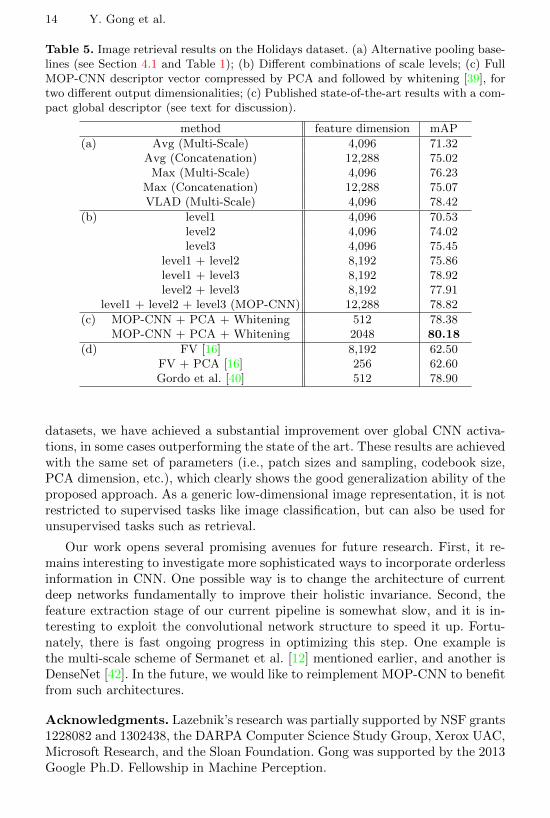
4.4 Image Retrieval Results

As our last experiment, we demonstrate the usefulness of our approach for an un-supervised image retrieval scenario on the Holidays dataset. Table 5 reports themAP results for nearest neighbor retrieval of feature vectors using the Euclideandistance. On this dataset, level1 is the weakest of all three levels because imagesof the same instance may be related by large rotations, viewpoint changes, etc.,and global CNN activations do not have strong enough invariance to handlethese transformations. As before, combining all three levels achieves the bestperformance of 78.82%. Using aggressive dimensionality reduction with PCAand whitening as suggested in [39], we can raise the mAP even further to 80.8%with only a 2048-dimensional feature vector. The state of the art performance onthis dataset with a compact descriptor is obtained by Gordo et al. [40] by usingFV/VLAD and discriminative dimensionality reduction, while our method stillachieves comparable or better performance. Note that it is possible to obtaineven higher results on Holidays with methods based on inverted files with verylarge vocabularies. In particular, Tolias et al. [41] report 88% but their repre-sentation would take more than 4 million dimensions per image if expanded intoan explicit feature vector, and is not scalable to large datasets. Yet further im-provements may be possible by adding techniques such as query expansion andgeometric verification, but they are not applicable for generic image representa-tion, which is our main focus. Finally, we show retrieval examples in Figure 7.We can clearly see that MOP-CNN has improved robustness to shifts, scaling,and viewpoint changes over global CNN activations.


Table 4. Classification results on ILSVRC2012/2013. (a) Alternative pooling baselines(see Section 4.1 and Table 1); (b) Different combinations of scale levels; (c) Numbersfor state-of-the-art CNN implementations. All the numbers come from the respectivepapers, except the Caffe numbers, which were obtained by us by directly testing theirfull network pre-trained on ImageNet. “Global” corresponds to testing on global imagefeatures, and “Center+Corner+Flip” corresponds to averaging the prediction scoresover ten crops taken from the test image (see Section 3 for details).


(c) Avg (Multi-Scale) 4096 53.34Avg (Concatenation) 12,288 56.12

Max (Multi-Scale) 4096 54.37Max (Concatenation) 12,288 55.88VLAD (Multi-Scale) 4,096 48.54




(c) Caffe (Global) [24] – 54.34Caffe (Center+Corner+Flip) [24] – 56.30

Krizhevsky et al. [2] – 59.93Zeiler and Fergus (6 CNN models) [22] – 64.00

OverFeat (1 CNN model) [12] – 64.26OverFeat (7 CNN models) [12] – 66.04

(a) Query (b) level1 (c) MOP-CNN

Fig. 7. Image retrieval examples on the Holiday dataset. Red border indicates a groundtruth image (i.e., a positive retrieval result). We only show three retrieved examplesper query because each query only has one to two ground truth images.

5 Discussion

This paper has presented a multi-scale orderless pooling scheme that is built ontop of deep activation features of local image patches. On four very challenging

14 Y. Gong et al.

Table 5. Image retrieval results on the Holidays dataset. (a) Alternative pooling base-lines (see Section 4.1 and Table 1); (b) Different combinations of scale levels; (c) FullMOP-CNN descriptor vector compressed by PCA and followed by whitening [39], fortwo different output dimensionalities; (c) Published state-of-the-art results with a com-pact global descriptor (see text for discussion).

method feature dimension mAP






(c) MOP-CNN + PCA + Whitening 512 78.38MOP-CNN + PCA + Whitening 2048 80.18

(d) FV [16] 8,192 62.50FV + PCA [16] 256 62.60Gordo et al. [40] 512 78.90

datasets, we have achieved a substantial improvement over global CNN activa-tions, in some cases outperforming the state of the art. These results are achievedwith the same set of parameters (i.e., patch sizes and sampling, codebook size,PCA dimension, etc.), which clearly shows the good generalization ability of theproposed approach. As a generic low-dimensional image representation, it is notrestricted to supervised tasks like image classification, but can also be used forunsupervised tasks such as retrieval.

Our work opens several promising avenues for future research. First, it re-mains interesting to investigate more sophisticated ways to incorporate orderlessinformation in CNN. One possible way is to change the architecture of currentdeep networks fundamentally to improve their holistic invariance. Second, thefeature extraction stage of our current pipeline is somewhat slow, and it is in-teresting to exploit the convolutional network structure to speed it up. Fortu-nately, there is fast ongoing progress in optimizing this step. One example isthe multi-scale scheme of Sermanet et al. [12] mentioned earlier, and another isDenseNet [42]. In the future, we would like to reimplement MOP-CNN to benefitfrom such architectures.

Acknowledgments. Lazebnik’s research was partially supported by NSF grants1228082 and 1302438, the DARPA Computer Science Study Group, Xerox UAC,Microsoft Research, and the Sloan Foundation. Gong was supported by the 2013Google Ph.D. Fellowship in Machine Perception.


References

1. LeCun, Y., Boser, B., Denker, J., Henderson, D., Howard, R., Hubbard, W., Jackel,L.: Handwritten digit recognition with a back-propagation network. In: NIPS.(1990)

2. Krizhevsky, A., Sutskever, I., Hinton, G.: Imagenet classification with deep convo-lutional neural networks. In: Advances in Neural Information Processing Systems25. (2012) 1106–1114

3. Goodfellow, I., Warde-Farley, D., Mirza, M., Courville, A., Bengio, Y.: Maxoutnetworks. In: ICML. (2013)

4. Le, Q., Ranzato, M., Monga, R., Devin, M., Chen, K., Corrado, G., Dean, J., Ng,A.: Building high-level features using large scale unsupervised learning. In: ICML.(2012)

5. Wan, L., Zeiler, M., Zhang, S., Lecun, Y., Fergus, R.: Regularization of neuralnetworks using DropConnect. In: ICML. (2013)

6. Hinton, G.E., Srivastava, N., Krizhevsky, A., Sutskever, I., Salakhutdinov, R.R.:Improving neural networks by preventing co-adaptation of feature detectors. Arxivpreprint arXiv:1207.0580 (2012)

7. Simonyan, K., Vedaldi, A., Zisserman, A.: Deep fisher networks for large-scaleimage classification. In: Proceedings Advances in Neural Information ProcessingSystems (NIPS). (2013)

8. Donahue, J., Jia, Y., Vinyals, O., Hoffman, J., Zhang, N., Tzeng, E., Darrell, T.:Decaf: A deep convolutional activation feature for generic visual recognition. arXivpreprint arXiv:1310.1531 (2013)

9. Girshick, R., Donahue, J., Darrell, T., Malik, J.: Rich feature hierarchies for accu-rate object detection and semantic segmentation. arXiv preprint arXiv:1311.2524(2013)

10. Oquab, M., Bottou, L., Laptev, I., Sivic, J., et al.: Learning and transferringmid-level image representations using convolutional neural networks. In: CVPR.(2014)

11. Razavian, A., Azizpour, H., Sullivan, J., Carlsson, S.: CNN features off-the-shelf:An astounding baseline for recognition. In: CVPR 2014 DeepVision Workshop.(2014)

12. Sermanet, P., Eigen, D., Zhang, X., Mathieu, M., Fergus, R., LeCun, Y.: Overfeat:Integrated recognition, localization and detection using convolutional networks.arXiv preprint arXiv:1312.6229 (2013)

13. Deng, J., Dong, W., Socher, R., Li, L.J., Li, K., Fei-Fei, L.: ImageNet: A large-scalehierarchical image database. In: CVPR. (2009)

14. Lazebnik, S., Schmid, C., Ponce, J.: Beyond bags of features: Spatial pyramidmatching for recognizing natural scene categories. In: CVPR. (2006)

15. Perronnin, F., Dance, C.R.: Fisher kernels on visual vocabularies for image cate-gorization. In: CVPR. (2007)

16. Jegou, H., Douze, M., Schmid, C., Perez, P.: Aggregating local descriptors into acompact image representation. In: CVPR. (2010) 3304–3311

17. Wang, J., Yang, J., Yu, K., Lv, F., Huang, T., Gong, Y.: Locality-constrainedlinear coding for image classification. CVPR (2010)

18. Csurka, G., Dance, C., Fan, L., Willamowski, J., Bray, C.: Visual categorizationwith bags of keypoints. In: ECCV Workshop on Statistical Learning in ComputerVision. (2004)

16 Y. Gong et al.

19. Sivic, J., Zisserman, A.: Video Google: A text retrieval approach to object matchingin videos. In: ICCV. (2003)

20. Grauman, K., Darrell, T.: The pyramid match kernel: Discriminative classificationwith sets of image features. In: In ICCV. (2005) 1458–1465

21. Lowe, D.G.: Distinctive image features from scale-invariant keypoints. IJCV 60(2)(2004) 91–110

22. Zeiler, M.D., Fergus, R.: Visualizing and understanding convolutional neural net-works. arXiv preprint arXiv:1311.2901 (2013)

23. Lee, H., Grosse, R., Ranganath, R., Ng, A.Y.: Convolutional deep belief networksfor scalable unsupervised learning of hierarchical representations. In: ICML. (2009)609–616

24. Jia, Y.: Caffe: An open source convolutional architecture for fast feature embed-ding. http://caffe.berkeleyvision.org/ (2013)

25. Bergamo, A., Sinha, S.N., Torresani, L.: Leveraging structure from motion to learndiscriminative codebooks for scalable landmark classification. In: Proceedings ofthe 2013 IEEE Conference on Computer Vision and Pattern Recognition. CVPR’13 (2013)

26. Perronnin, F., Sanchez, J., Mensink, T.: Improving the Fisher kernel for large-scaleimage classification. In: ECCV. (2010)

27. Perronnin, F., Liu, Y., Sanchez, J., Poirier, H.: Large-scale image retrieval withcompressed Fisher vectors. In: CVPR. (2010)

28. Xiao, J., Hays, J., Ehinger, K.A., Oliva, A., Torralba, A.: SUN database: Large-scale scene recognition from abbey to zoo. In: CVPR. (2010) 3485–3492

29. Pandey, M., Lazebnik, S.: Scene recognition and weakly supervised object local-ization with deformable part-based models. In: ICCV. (2011) 1307–1314

30. Quattoni, A., Torralba, A.: Recognizing indoor scenes. In: CVPR. (2009)

31. Deng, J., Berg, A., Satheesh, S., Su, H., Khosla, A., Fei-Fei, L.: Large scale vi-sual recognition challenge. http://www.image-net.org/challenges/LSVRC/2012/(2012)

32. Russakovsky, O., Deng, J., Huang, Z., Berg, A., Fei-Fei, L.: Detecting avocados tozucchinis: what have we done, and where are we going? In: ICCV. (2013)

33. Jegou, H., Douze, M., Schmid, C.: Hamming embedding and weak geometricconsistency for large-scale image search. In: ECCV. (2008)

34. Akata, Z., Perronnin, F., Harchaoui, Z., Schmid, C., et al.: Good practice in large-scale learning for image classification. PAMI (2013)

35. Sanchez, J., Perronnin, F., Mensink, T., Verbeek, J.: Image Classification with theFisher Vector: Theory and Practice. IJCV 105(3) (2013) 222–245

36. Singh, S., Gupta, A., Efros, A.A.: Unsupervised discovery of mid-level discrimina-tive patches. In: ECCV. (2012)

37. Juneja, M., Vedaldi, A., Jawahar, C.V., Zisserman, A.: Blocks that shout: Distinc-tive parts for scene classification. In: CVPR. (2013)

38. Doersch, C., Gupta, A., Efros, A.A.: Mid-level visual element discovery as discrim-inative mode seeking. In: NIPS. (2013)

39. Jegou, H., Chum, O.: Negative evidences and co-occurrences in image retrieval:the benefit of PCA and whitening. In: ECCV. (2012)

40. Gordo, A., Rodrıguez-Serrano, J.A., Perronnin, F., Valveny, E.: Leveragingcategory-level labels for instance-level image retrieval. In: CVPR. (2012)

41. Tolias, G., Avrithis, Y., Jegou, H.: To aggregate or not to aggregate: selectivematch kernels for image search. In: ICCV. (2013)


42. Iandola, F., Moskewicz, M., Karayev, S., Girshick, R., Darrell, T., Keutzer, K.:DenseNet: Implementing efficient convnet descriptor pyramids. arXiv preprintarXiv:1404.1869 (2014)

Multi-Scale Orderless Pooling of Deep Convolutional...

Documents

Transcript of Multi-Scale Orderless Pooling of Deep Convolutional...