Pacific Graphics 2010P. Alliez, K. Bala, and K. Zhou(Guest Editors)

Volume 29 (2010), Number 7

Multi-Resolution Cloth Simulation

Yongjoon Lee 1 Sung-eui Yoon 1 Seungwoo Oh 2 Duksu Kim 1 Sunghee Choi 1

1 KAIST (Korea Advanced Institute of Science and Technology)2 CLO Virtual Fashion Inc.

AbstractWe propose a novel, multi-resolution method to efficiently perform large-scale cloth simulation. Our cloth simula-tion method is based on a triangle-based energy model constructed from a cloth mesh. We identify that solutionsof the linear system of cloth simulation are smooth in certain regions of the cloth mesh and solve the linear systemon those regions in a reduced solution space. Then we reconstruct the original solutions by performing a sim-ple interpolation from solutions computed in the reduced space. In order to identify regions where solutions aresmooth, we propose simplification metrics that consider stretching, shear, and bending forces, as well as geomet-ric collisions. Our multi-resolution method can be applied to many existing cloth simulation methods, since ourmethod works on a general linear system. In order to demonstrate benefits of our method, we apply our methodinto four large-scale cloth benchmarks that consist of tens or hundreds of thousands of triangles. Because of thereduced computations, we achieve a performance improvement by a factor of up to one order of magnitude, witha little loss of simulation quality.

Categories and Subject Descriptors (according to ACM CCS): I.3.5 [Computer Graphics]: Computational Geometryand Object Modeling—Physically based modeling

1. Introduction

Cloth simulation has been extensively researched in orderto achieve realistic simulations of various fabrics. Sincemost fabrics are very flexible and do not have elasticity, themeshes resulted from realistic cloth simulations can havehighly detailed features such as wrinkles. Therefore, the res-olutions of meshes used for high-quality cloth simulationsare typically very high enough to capture such detailed fea-tures. However, using such high resolution meshes can causesignificantly slow simulation performances, especially sincethe time complexity of most high-quality cloth simulationsis higher than linear functions with the number of vertices ofthe mesh [GHF∗07].

Many orthogonal approaches have been proposed to ac-celerate the performance of cloth simulation. At a high level,they include allowing larger time steps [BW98], GPU-basedparallelization [Gre03], wrinkle synthesis [WHRO10], fastercollision detection [KHH∗09,GKJ∗05], and multi-resolutionapproaches [VB05].

Existing multi-resolution techniques [VB05, HPH96]achieve a higher simulation performance by providing adap-tive meshes. These techniques identify mesh regions thatrequire high accuracy and use more high resolutions onlyfor those regions instead of using a uniformly refined mesh.However, existing multi-resolution techniques do not at-tempt to simplify mesh regions where can be represented

(a) (b)

Figure 1: The left figure shows simulation of a dress in a woman,who is not shown in this figure. The right figure shows the multi-resolution mesh used to perform the simulation at a particularframe. The original dress mesh has 25 K vertices. By simplifyingdynamically smooth regions of the dress mesh, our method achieves9 times performance improvement by reducing 73.8% of the verticesof the original mesh.

c© 2010 The Author(s)Journal compilation c© 2010 The Eurographics Association and Blackwell Publishing Ltd.Published by Blackwell Publishing, 9600 Garsington Road, Oxford OX4 2DQ, UK and350 Main Street, Malden, MA 02148, USA.

Y. Lee et al. / Multi-Resolution Cloth Simulation

with lower resolutions while providing plausible simulationquality. Moreover, these techniques have been designed onlyfor mass-spring models and are not directly applicable tomore general cloth models [BW98,CK02,GHF∗07] that arewidely used for high-quality cloth simulation.

Main contributions: In this paper we propose a novel multi-resolution cloth simulation method that simplifies linear sys-tem that do not require a high resolution, in order to improvethe performance of cloth simulation while maintaining thesimulation quality. We design our multi-resolution approachfor a triangle-based energy model with implicit Euler inte-gration. We identify that solutions of the linear system ofcloth simulations are smooth in certain regions and solve thelinear system in a reduced solution space. Then we constructthe original solutions by performing a simple interpolation.In order to identify regions whose solutions for the linearsystem are smooth, we use simplification metrics that con-sider various forces and geometric collisions. We have im-plemented our method and applied it to various cloth bench-marks consisting of up to 100 K vertices. With a little lossof simulation quality, our method achieves the performanceimprovement by a factor of up to one order of magnitudewith our tested benchmarks.

2. Related WorkIn this section we review prior work on cloth simulation andits various acceleration techniques.

2.1. Cloth SimulationThe cloth simulation has been extensively researchedand good surveys [CK05] are available. Since Breen etal. [BHW94] proposed a particle based cloth model, themass-spring model has been widely used for efficient and re-alistic cloth simulation. Provot [Pro96] introduced a simplemass-spring model and an explicit integration-based solver.Although this method runs interactively, it suffers from un-stable behaviors as the time step becomes large. For a ro-bust cloth simulation even with large time steps, Baraff andWitkin [BW98] developed an implicit integration method.Choi and Ko [CK02] improved the stability and quality ofsimulation by introducing an immediate buckling model.Also, Bridson et al. [BFA02] proposed a robust method thathandles various contacts. Goldenthal et al. [GHF∗07] ad-dressed the over-stretched problem of cloth based on con-strained Lagrangian mechanics to constrain the distance be-tween particles. Wang et al. [WHRO10] recently proposedan example-based wrinkle synthesis technique, which com-bines fine wrinkles with coarse cloth simulation. Aguiaret al. [dASTH10] presented a learning-based approach tomodel the dynamic behavior of clothes and used it for ef-ficient cloth simulation.

2.2. Adaptive Cloth SimulationMany adaptive techniques have been proposed to improvethe performance and quality of cloth simulations. Hutchin-son et al. [HPH96] and Zhang et al. [ZY01] proposed adap-tive cloth simulation methods based on the mass-spring

model. These methods treat the mass-spring model of a clothas a mesh and refine a portion of the mesh that requiresa higher mesh resolution. However, these methods showedmuch lower simulation quality compared to using a uniformmesh that has a higher resolution. Villard et al. [VB05] alsoproposed an adaptive meshing method. This method pre-served the force momentum during the refinement of theadaptive mesh and thus achieved a simulation quality sim-ilar to that of the original cloth simulation that use uni-form meshes. However, all these prior adaptive techniquesare based on the mass-spring model and are not easily ap-plicable to other types of cloth models (e.g., triangle-basedenergy models [BW98]) that can show high cloth simulationquality.

2.3. Adaptive Techniques in Other Fields

Adaptive techniques have been extensively studied in vari-ous simulations. Grinspun et al. [GKS02] addressed adap-tive simulation for finite element methods by refinement ofbasis functions. An et al. [AKJ08] use optimized cubaturesto reduce the size of various linear equation systems. Theirmethod requires a training set to compute optimized cuba-tures.

Losasso et al. [LGF04] use an octree data structure to sim-ulate water and smoke efficiently. They discretize the linearsystem on an unrestricted octree grid so that they reduce thesize of the linear system. Agarwala [Aga07] apply this ideato constructing a seamless large-scale image panorama thatrequires solving the Poisson equation. He reduces the size ofthe linear system drastically, since the solutions for the Pois-son equations are smooth. Our method is inspired by thisadaptive method that reduces the size of the linear system bymerging smooth solutions into one.

2.4. Multigrid Methods

Multigrid methods have been widely used in many differ-ent simulations. Its main idea is to accelerate the conver-gence of a basic iterative method, accomplished by solv-ing a problem with regularly, coarser domains in multiplelevels. However, these multigrid methods have not been ac-tively employed in cloth simulation, mainly because the sim-ulated cloth meshes have many fine details such as wrin-kles. Müller [Mül08] simulated clothes with a hierarchi-cal multigrid solver for a position-based dynamics. Oh etal. [ONW08] applied the physically faithful standard v-cyclemultigrid to cloth simulation. Our method shows more effi-ciency than this standard multigrid method for cloth simula-tion.

3. Overview

In this section, we give an overview of our approach to effi-ciently simulate large-scale clothes.

3.1. Issues of Large-Scale Cloth Simulations

Cloth is highly constrained because of inextensibility andcollision constraint. The reality of cloth simulation depends

c© 2010 The Author(s)Journal compilation c© 2010 The Eurographics Association and Blackwell Publishing Ltd.

Y. Lee et al. / Multi-Resolution Cloth Simulation

Smoothness of velocity

In-planedeformation

Out-planedeformation

Collision status

simplify

Figure 2: This figure shows an overview of our approach. We con-sider a mesh region to be dynamically smooth, if the mesh regionhas smooth in-plane deformations (e.g., stretching and shearing),smooth out-of-plane deformation (e.g., bending), and smooth veloc-ities at the current frame. Given a cloth mesh, we check whethera mesh region is dynamically smooth and its collision status is notchanged from the previous frame. If so, we simplify the linear equa-tions related to dynamically smooth regions, leading to a higher per-formance for cloth simulation.

on how well we satisfy these constraints. Many cloth sim-ulations construct constraints-integrated linear systems andthen use a solver to obtain adequate solutions for those lin-ear systems. Iterative solvers like conjugate gradient [HS52,She94] have been widely used to solve those linear systems.

For a large-scale cloth, we find that even iterative solverslike the preconditioned conjugate gradient (PCG) can takea huge amount of time, since PCG, one of most efficient it-erative solvers, has a time complexity of O(n1.5) to solve a3n× 3n linear system. For example, solving a linear systemfor a cloth mesh consisting of 100 K vertices takes about 20seconds on our test machine.

3.2. Our Approach

The main idea of our approach is to reduce the size of lin-ear system by utilizing the smoothness of solutions of thesystem (Sec. 4.1) with adaptive meshes. First, we constructthe original linear system with a high-resolution cloth mesh.This original linear system contains the full information ofthe high-resolution cloth mesh. Then we consider variousforces and collisions to simplify the solutions of portions ofthe cloth mesh, leading to a reduced linear system (Sec. 4.2and Sec. 4.3). We then solve the simplified linear system ina reduced solution space and reconstruct the original solu-tions based on a simple linear interpolation from the solu-tions computed in the reduced space (Sec. 4.4). Finally, weemploy an error correction with a few iterations on the resid-ual equation to reduce high-frequency error (Sec. 4.5). Theoverview of our approach is shown in Fig. 2.

Notations Throughout the paper, we use italic capital lettersto denote triangles (T ), bold capital letters to denote matri-ces (M), bold small letters to denote vectors (v), and italicsmall letters to denote scalars (s). Superscript(t ) indicates theframe number.

4. Adaptive Cloth Simulation

We assume in this paper that cloth simulation method uses atriangle-based energy model constructed from a cloth mesh,integrated with the well-known implicit Euler integrationmethod [BW98]. However, our method can be easily ex-tended to other types (e.g., mass-spring model) of energymodels and other integration methods, if one can design alinear system from those cloth models and integration meth-ods.

The implicit Euler integration for the triangle-based en-ergy model from a cloth mesh gives the following linearequations [BW98]:(

M−h(

∂f∂v

+h∂f∂x

))∆v = h

(ft +h

∂f∂x

vt), (1)

where h is a length of time step, M is a mass matrix, f isa force vector, x and v are position and velocity vectors de-fined for each vertex of the cloth mesh, and ∆v is a differencebetween two velocities of vt+1/2 and vt †.

Eq. (1) can be rewritten as the following standard linearsystem using the fact that ∆x = h ·vt+1/2:

A∆x = b (2)

We perform our simplification method in the space of ∆x,instead of ∆v, since ∆x is likely to be smooth for regions ofthe cloth mesh, even though ∆v varies for those regions.

4.1. Dynamically Smooth Regions

Even though the cloth mesh can have very complex geomet-ric shapes such as wrinkles, velocities ∆x on portions of themesh can vary smoothly.

In order to identify mesh regions that can be simplifiedwith our method, we decompose the mesh into the followingtwo regions: dynamically smooth and complex regions. Intu-itively speaking, a mesh region belongs to the dynamicallysmooth regions, if all the vertices of the mesh region havesimilar velocities ∆x.

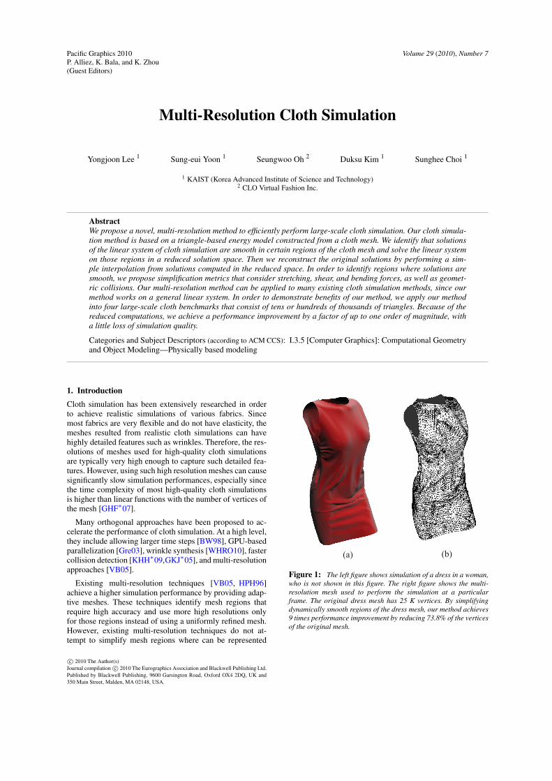
Fig. 3 shows an example of the cloth mesh with regionsthat can be classified as dynamically smooth regions andthus can be simplified with our method. In this example, aball collides with a cloth and pushes it. Fig. 3-(b) shows ve-locities of each vertex, each of whose x, y, and z compo-nents is visualized in the red, green, and blue channels re-spectively. In the example cloth mesh, region 2 that has verysmooth geometry and also has very smooth velocities. Also,region 1 that has a wrinkled region, a complex geometry,also has similar velocities. Therefore, region 1 and 2 can beclassified as dynamically smooth regions. However, region 3that has different velocities is classified as the dynamicallycomplex region and thus is not simplified in our method.

† vt+1/2 is an updated velocity with the information (e.g., veloci-ties, forces and Jacobians) of frame t. vt+1 is then calculated withvt+1/2 and the collision information of frame t.

c© 2010 The Author(s)Journal compilation c© 2010 The Eurographics Association and Blackwell Publishing Ltd.

Y. Lee et al. / Multi-Resolution Cloth Simulation

(a) (b)

Figure 3: In the left figure (a), a ball collides with a clothmesh. The right figure (b) shows the velocities of the mesh,each of whose x, y, and z components maps to the red, green,and blue channels respectively.

Once we identify dynamically smooth regions, we sim-plify linear equations related to those regions and solve so-lutions for the simplified equations in a reduced space, ∆y,instead of the original space ∆x. Then, ∆x that are simplifiedinto ∆y can be computed by interpolating elements of ∆y.For this, we introduce a transformation matrix, S, that trans-forms a reduced space, ∆y, to the solution space, ∆x of theoriginal linear equations. As a result, Eq. 2 is transformedinto the following equation:

AS∆y = b, (3)

where ∆x = S∆y, and ∆y is a vector of length O(m), whichis much smaller than the length O(n) of the vector ∆x.

4.2. Construction of Multi-Resolution Representation

In order to efficiently perform the simplification on the dy-namically smooth regions, we utilize a multi-resolution rep-resentation built from an input cloth mesh.

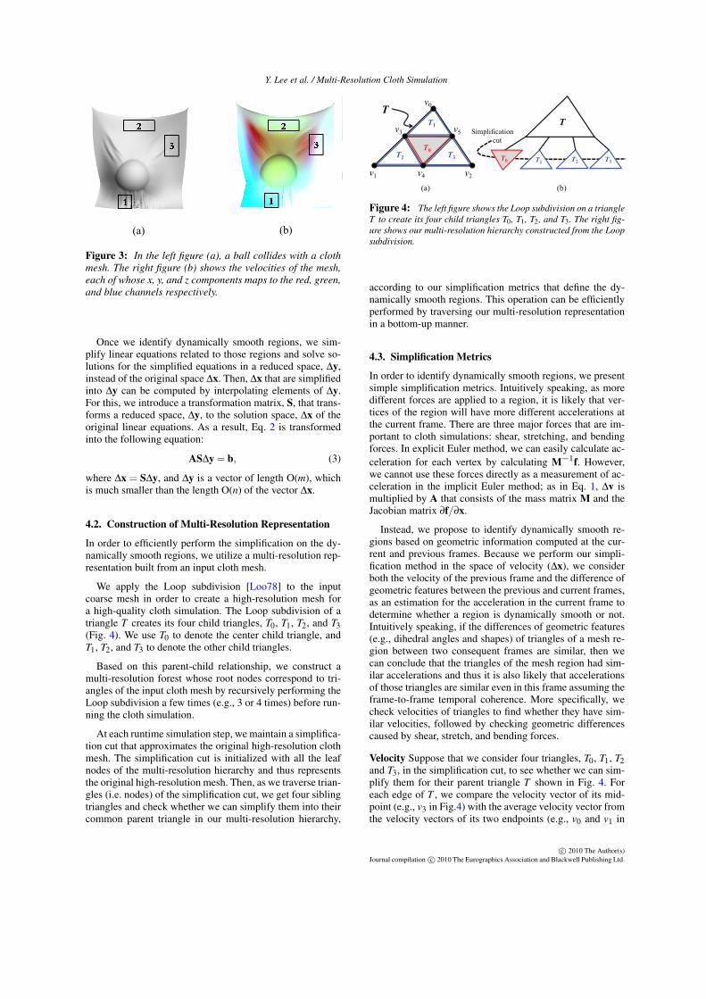
We apply the Loop subdivision [Loo78] to the inputcoarse mesh in order to create a high-resolution mesh fora high-quality cloth simulation. The Loop subdivision of atriangle T creates its four child triangles, T0, T1, T2, and T3(Fig. 4). We use T0 to denote the center child triangle, andT1, T2, and T3 to denote the other child triangles.

Based on this parent-child relationship, we construct amulti-resolution forest whose root nodes correspond to tri-angles of the input cloth mesh by recursively performing theLoop subdivision a few times (e.g., 3 or 4 times) before run-ning the cloth simulation.

At each runtime simulation step, we maintain a simplifica-tion cut that approximates the original high-resolution clothmesh. The simplification cut is initialized with all the leafnodes of the multi-resolution hierarchy and thus representsthe original high-resolution mesh. Then, as we traverse trian-gles (i.e. nodes) of the simplification cut, we get four siblingtriangles and check whether we can simplify them into theircommon parent triangle in our multi-resolution hierarchy,

T

(a) (b)

T0T2

v0

v1

v3T1

T0

v5

v4 v2

T

T1 T2 T3T0

Simplificationcut

T3

Figure 4: The left figure shows the Loop subdivision on a triangleT to create its four child triangles T0, T1, T2, and T3. The right fig-ure shows our multi-resolution hierarchy constructed from the Loopsubdivision.

according to our simplification metrics that define the dy-namically smooth regions. This operation can be efficientlyperformed by traversing our multi-resolution representationin a bottom-up manner.

4.3. Simplification Metrics

In order to identify dynamically smooth regions, we presentsimple simplification metrics. Intuitively speaking, as moredifferent forces are applied to a region, it is likely that ver-tices of the region will have more different accelerations atthe current frame. There are three major forces that are im-portant to cloth simulations: shear, stretching, and bendingforces. In explicit Euler method, we can easily calculate ac-celeration for each vertex by calculating M−1f. However,we cannot use these forces directly as a measurement of ac-celeration in the implicit Euler method; as in Eq. 1, ∆v ismultiplied by A that consists of the mass matrix M and theJacobian matrix ∂f/∂x.

Instead, we propose to identify dynamically smooth re-gions based on geometric information computed at the cur-rent and previous frames. Because we perform our simpli-fication method in the space of velocity (∆x), we considerboth the velocity of the previous frame and the difference ofgeometric features between the previous and current frames,as an estimation for the acceleration in the current frame todetermine whether a region is dynamically smooth or not.Intuitively speaking, if the differences of geometric features(e.g., dihedral angles and shapes) of triangles of a mesh re-gion between two consequent frames are similar, then wecan conclude that the triangles of the mesh region had sim-ilar accelerations and thus it is also likely that accelerationsof those triangles are similar even in this frame assuming theframe-to-frame temporal coherence. More specifically, wecheck velocities of triangles to find whether they have sim-ilar velocities, followed by checking geometric differencescaused by shear, stretch, and bending forces.

Velocity Suppose that we consider four triangles, T0, T1, T2and T3, in the simplification cut, to see whether we can sim-plify them for their parent triangle T shown in Fig. 4. Foreach edge of T , we compare the velocity vector of its mid-point (e.g., v3 in Fig.4) with the average velocity vector fromthe velocity vectors of its two endpoints (e.g., v0 and v1 in

c© 2010 The Author(s)Journal compilation c© 2010 The Eurographics Association and Blackwell Publishing Ltd.

Y. Lee et al. / Multi-Resolution Cloth Simulation

Fig. 4). If these two velocities are similar in terms of themagnitude and direction of these two velocities, we furthercheck in-plane and out-of-plane deformations for the sim-plification. Otherwise, we do not simplify the four triangles.Then, we fetch other four triangles in the simplification cutand continue to check them for the simplification.

In-plane deformation In-plane deformation on clothmeshes is governed by stretch and shear forces. If strongin-plane forces are exerted on a triangle, those forces de-form the triangle along the in-plane direction. For estimatingstretch and shear forces, we check the difference of stretchfactor (wu, wv) and shear factor (wu+v, wu−v) during a timestep [BW98]. We can calculate wu and wv of triangle Ti jkconsisting of vertices i, j,k as

(wu wv) =(x j−xi xk−xi

)(u j−ui uk−ui

)−1,

where xi is the position of vertex i in the world coordinate,ui is the rest position of vertex i in the 2D-domain coordi-nate. We can calculate wu+v, wu−v by wu+v = wu +wv, andwu−v = wu−wv [CK02, ONW08]. We then define our sim-plification metrics for stretching and shearing at frame t asfollows :

Mtstretch(T ) = A(T )

∆|wtu|+∆|wt

v|h

Mtshear(T ) = A(T )

∆|wtu+v|+∆|wt

u−v|h

,

where A(T ) is the area of triangle T and ∆|wt | = |wt | −|wt−1|. Since as the area of a triangle becomes larger andthe difference becomes larger at a unit time, there are morestretching and shearing forces on the triangle, we considerthem in our simplification metrics.

Out-of-plane deformation In order to estimate the differ-ence of the bending force between two neighboring trian-gles, we consider the difference of the dihedral angle ofthose two neighboring triangles at the previous and currentframes. We use ∠tTj to denote the angle between two trian-gles T0 and Tj at frame t, shown in Fig. 4. Then the simplifi-cation metric for the bending force of a triangle T at frame tis defined as the following:

Mtbend(T ) = max

j=1,2,3A(T )

∆∠tTj

h,

where ∆∠tTj is the difference between ∠t−1Tj and ∠tTj.The area of a triangle A(T ) is also considered as in the in-plane deformation.

Collisions Our simplification metrics for shear, stretch, andbending forces are based on the frame-to-frame temporal co-herence. However, once we have self-collisions within thecloth mesh or inter-collisions between the cloth mesh andother objects, the frame-to-frame temporal coherence is notsatisfied. Also, the frame-to-frame coherence breaks evenwhen collisions among meshes are resolved. Therefore, wedo not simplify vertices or triangles at the moment whentheir collision states are changed.

0.02

0.04

0.06

0.08

0.1

0.12

0.14

0.16

0 10 20 30 40 50 60 70 80 90 100

Erro

r (m

m)

Number of iterations for the error correction

L2 norm of meanVariance

(a)

(b)

(c)

Figure 5: (a) Mean and variance of errors caused by our ap-proach. The variance of errors is drastically reduced by a few itera-tions of our error correction method. (b) and (c) show errors beforeand after performing the error correction step with 10 iterations re-spectively. x, y, and z components of errors map to red, green, andblue respectively.

4.4. Computing Simplified Solutions

We first construct the transformation matrix S according toour simplification metrics, by traversing our multi-resolutionhierarchy in a bottom-up manner. Then we compute solu-tions of the linear system defined in a reduced solution space.

Formulating the transformation matrix S We traverse ourmulti-resolution hierarchy in a bottom-up manner to con-struct the simplification cut that represents the simplifiedcloth mesh at the current frame. Once we compute the sim-plification cut, then we can formulate the transformation ma-trix S. The original solutions in the space of ∆x can be repre-sented by a weighted sum of simplified solutions computedin the space of ∆y. For example, suppose that we simplifyfour sibling triangles, T0, T1, T2, and T3, shown in Fig. 4 intotheir parent triangle T . Once we compute solutions for v0,v1, and v2 for the parent triangle T , then the solution of v3can be computed by the average of solutions of v0 and v1;solutions of other vertices v4 and v5 can be computed in asimilar manner.

Solving the reduced linear system In order to solve the lin-ear system of Eq. 3 that is defined in the reduced solutionspace, we multiply ST to both sides of the equation, result-ing in the following equation:

ST AS∆y = ST b. (4)

The size of ST AS becomes 3m× 3m, where m is the num-ber of vertices of the simplified cloth mesh. We use PCG tosolve Eq. 4. Computing ST AS can be done quickly, since Aand S are sparse. For a cloth that consists of 20 K triangles,computing ST AS takes only 10 ms to 15 ms, while solvingthe original linear system takes 500 ms to 1000 ms.

4.5. Error Correction

We approximate the original solution, ∆xsol , of Eq. 2, asthe product of S and the solution, ∆ysol of Eq. 4. However,S∆ysol is not exactly the same as ∆xsol , resulting in error, e.

c© 2010 The Author(s)Journal compilation c© 2010 The Eurographics Association and Blackwell Publishing Ltd.

Y. Lee et al. / Multi-Resolution Cloth Simulation

(a) (b)

(c) (d)

Figure 6: This figure shows our tested benchmark models: a rect-angular shape cloth (a), a cloth with a ball (b), a walking woman ina dress (c), and a walking man in trousers (d).

Especially, it is likely that the error becomes bigger when wehave collisions, which breaks the frame-to-frame coherence.

The error e consists of high-frequency errors (e.g., bumpsand unrealistic wrinkles) and low-frequency errors (e.g., theoverall shape of cloth). Artifacts caused by high-frequencyerrors look more unpleasant than those caused by low-frequency errors.

In order to reduce errors, especially visually unpleasanthigh-frequency errors, we perform error correction with theresidual equation. We formulate the residual equation of Eq.2 as the following:

Ae = b−AS∆y. (5)

As we perform iterations with PCG on Eq. 5, high-frequency errors drastically decrease with only a few iter-ations [Wes92]. Fig. 5-(a) shows the mean and variance oferrors on a frame of one of our benchmarks. Note that thevariance of errors are drastically reduced by only a few iter-ations.

5. Results

We have implemented our method on a PC with a 3.0GHzIntel CPU, an NVIDIA GeForce 8800 GTX, and 2GB main

memory. For collision detection, we use a hybrid parallelcontinuous collision detection method [KHH∗09]. To handlecollisions, we use the velocity filtering with the repulsionforce method as proposed by Bridson et al.’s [BFA02].

We test our method with four different benchmarks (Fig.6). Our two benchmarks are simple cases: draping a rectan-gular cloth with two fixed points (Fig. 6-(a)), a cloth drapingon a ball (Fig. 6-(b)), a walking woman in a dress (Fig. 6-(c)), and a walking man in trousers (Fig. 6-(d)).

In order to define dynamically smooth regions, we usethe following thresholds. If the magnitudes of two veloc-ity vectors are within 10% difference and their angle is lessthan 0.056π, we consider them to be similar. Also, we use0.0001m2/s as a thresholds for both Mstretch and Mshear, and0.0013πm2/s as a threshold for Mbend . We perform 5 to 10iterations for the error correction; we use 5 iterations for sub-division level 3, and use 10 iterations for subdivision level 4.

We use 0.01s time step size for simulating benchmarksshown in Fig. 6-(a) and 6-(b). However, we use 0.001s timestep size for simulating benchmarks shown in Fig. 6-(c) and6-(d), since these two benchmarks have complex contactsbetween the cloth meshes and walking characters. Initialcloth meshes in these benchmarks are designed in low reso-lutions and thus are inappropriate for high-quality cloth sim-ulation. Therefore, we perform the Loop subdivision recur-sively 3 or 4 times to the base mesh. Also, during the re-finement process, we build our multi-resolution hierarchy asmentioned in Sec. 4.2.

Table 1 shows the average simulation time (excludingtime spent on collision detection and handling) of ourmethod and PCG with tested benchmarks. Overall ourmethod achieves 8 times on average with all the testedbenchmarks and up to 13 times performance improvementover using PCG with the original linear system. Also, as thecomplexity of cloth meshes increases, we observe that ourmethod shows higher performance improvements over PCG.Although our method approximates the solutions of the orig-inal linear equations, we found that there are little noticeablevisual artifacts and the simulation results of our method issimilar to those computed by PCG.

Our method has four main components: 1) initializingand setting up the linear equation (Init), 2) performing thesimplification and constructing the transformation matrix(Simp), 3) performing PCG in the reduced solution space(Solve), and 4) performing the error correction (EC). Wemeasure how much each component takes over the total sim-ulation time. Solve takes the biggest portion (e.g., 40% to50%) and other components take similar portions.

We also measure how many triangles of each subdivisionlevel are used in the benchmark of the walking woman witha dress that has the subdivision level of 4 in the original high-resolution mesh. 68% and 22% of triangles of the simplifiedcloth mesh have subdivision levels of 3 and 4 respectively.Other triangles are drastically simplified to have subdivisionlevels of 1 and 2.

c© 2010 The Author(s)Journal compilation c© 2010 The Eurographics Association and Blackwell Publishing Ltd.

Y. Lee et al. / Multi-Resolution Cloth Simulation

Scene Subd. Mat. No. vertices Total Ratio Iter. Average time of our method (ms) PCGlevel / No. triangles frames (%) Init Simp Solve EC Total (ms)

Figure 6-(a) 3 silk 5k/13k 300 11.61 5 16.8 14.3 34.0 15.0 80.1 471.84 silk 20k/52k 300 3.73 10 69.3 59.0 54.6 111.3 294.2 3805.2

Figure 6-(b) 3 cotton 9k/22k 300 25.04 5 17.0 14.5 86.9 13.4 131.8 1018.94 cotton 24k/61k 300 12.33 10 70.2 58.9 336.9 109.7 575.7 4312.3

Figure 6-(c) 3 silk 46k/90k 6000 26.18 5 89.0 68.3 273.3 74.2 504.8 2867.24 silk 121k/240k 6000 11.92 10 356.8 282.9 1562.9 542.7 2745.3 23055.2

Figure 6-(d) 3 leather 62k/122k 6000 16.05 5 119.4 97.3 391.5 84.2 692.4 7695.5

Table 1: This table shows the model complexity, material type, the subdivision level to compute the highest resolution, the average simplifi-cation ratio in terms of the number of vertices, and the total number of frames for each tested benchmark. We also show the average simulationtime for our method and PCG applied to the original linear system. Init – Initializing and setting up the linear system of Eq.2; Simp – Per-forming the simplification and constructing the transformation matrix; Solve – Solving Eq.4 with PCG; EC – Performing the error correction.Iter is the number of iterations for the error correction, PCG is time spent on performing PCG to the original linear system of Eq. 2.

5.1. Discussion

Time complexity The error correction has O(kn) time com-plexity [She94], where n is the number of vertices in theoriginal high-resolution mesh and k is the number of itera-tions for the error correction. Therefore, the time complexityof our overall approach is O(m1.5+kn), where m is the num-ber of vertices in the simplified mesh. In practice, m is muchsmaller than n (e.g., less than 30% of n for our benchmarks)and we use only 5 to 10 iterations for the error correction.As a result, we are able to observe 8 times performance im-provement on average over using PCG to the original linearsystem.

Comparison with the standard multigrid method Themain difference between our method and the standard multi-grid is that our method uses adaptive meshes for the sim-plification according to our simplification metrics, whereasthe multigrid uses uniform regular grids with v- or w-cycles.Such uniform grids may require many iterations for eachstep of v- or w-cycles for fine deformations of clothes.Therefore, our method can converge to a solution faster thanthe multigrid method in a short amount of time. To verifythis, we show simulation results (Fig. 7) computed from ourmethod and the standard v-cycle multigrid method [Wes92].Given the same computation time, our method produces asimulation result (Fig. 7-(b)) that is similar to one computedby solving the original linear equation with PCG (Fig. 7-(a)),while the multigrid method shows very different result (Fig.7-(c)). To achieve similar simulation quality, the multigrid(Fig. 7-(d)) takes much more time than ours (Fig. 7-(b)).

Limitations We assume that an input high resolution meshfor our method is computed by performing the Loop sub-division to a coarse mesh. We chose this approach, mainlybecause existing cloth meshes are not designed in high-resolutions and performing the Loop subdivision producessuch high quality cloth meshes while facilitating to con-struct our multi-resolution hierarchy. However, one can sim-plify an arbitrary input high-resolution mesh by using thewell-known edge-collapse simplification operator based onour simplification metrics. We have performed error correc-tion steps with a few iterations (e.g., 5 to 10), in order tomainly reduce the visually unpleasant high-frequency errors

(a)

(c) (d)

(b)

(a) (b) (c) (d)Solver PCG Our method Multigrid MultigridNum. of iterations - - 15 150on smoothingElapsed time(ms) 4312.3 575.7 574.9 3488.7

Figure 7: The four images show the simulation results on clothwith a ball (Fig. 6-(b)) on a frame 25. For adjusting the simulationquality of the multigrid, we modify the number of fixed iterations ofthe smoothing process with the standard V-cycle, as shown above inthe table.

in an efficient manner. However, low-frequency errors mayremain and thus it is possible to have artifacts on the simula-tion results.

6. Conclusion

We have designed an efficient multi-resolution cloth simu-lation technique. We identify dynamically smooth regionsand simplify those regions in order to improve the simulationperformance without deteriorating the simulation quality. Inorder to identify such dynamically smooth regions, we haveproposed simplification metrics that consider geometric con-

c© 2010 The Author(s)Journal compilation c© 2010 The Eurographics Association and Blackwell Publishing Ltd.

Y. Lee et al. / Multi-Resolution Cloth Simulation

tacts as well as various forces that govern energy-based clothmodels. As a result, we were able to observe 8 times perfor-mance improvement on average with the tested benchmarksover running the PCG to the original linear system.

There are many avenues for future research directions. Inour current method, we have only designed multi-resolutionapproach for solving the linear system of cloth simulation.We believe that we can further improve the performance ofthe cloth simulation by applying multi-resolution collisiondetection method [YSLM04] without generating unpleasantvisual artifacts. Also, we would like to improve the perfor-mance of our method by utilizing parallel many-core CPUsand GPUs. Since the main bottleneck of our method is onperforming PCG with the linear system even in the reducedsolution space, GPU-based parallel solvers [BFGS03] canfurther improve the performance of our method. Currently,we do not utilize any temporal coherences when we com-pute the simplified solutions. We believe that we can furtherimprove the performance of our method by utilizing tempo-ral coherences in a similar manner used in progressive de-forming meshes [HCC06]. Finally, we would like to sup-port tearing within our method. Since tearing of clothes re-quires high-resolution on the tearing boundary, we believethat our multi-resolution framework is very promising tosupport such effects.

Acknowledgment

We would like to thank anonymous reviewers fortheir constructive feedbacks. This project was sup-ported in part by MKE/MCST/IITA [2008-F-033-02],MKE/IITA u-Learning, MKE digital mask control,MCST/KOCCA-CTR&DP-2009, KRF-2008-313-D00922,KMCC, BK, DAPA/ADD (UD080042AD), MKE/KEIT[KI001810035261], and MSRA.

References[Aga07] AGARWALA A.: Efficient gradient-domain compositing

using quadtrees. ACM Trans. on Graphics 26, 3 (2007), 94. 2[AKJ08] AN S. S., KIM T., JAMES D. L.: Optimizing cubature

for efficient integration of subspace deformations. ACM Trans.on Graphics 27, 5 (2008), 165. 2

[BFA02] BRIDSON R., FEDKIW R., ANDERSON J.: Robust treat-ment for collisions, contact and friction for cloth animation. Proc.of ACM SIGGRAPH (2002), 594–603. 2, 6

[BFGS03] BOLZ J., FARMER I., GRINSPUN E., SCHRÖDER P.:Sparse matrix solvers on the gpu: conjugate gradients and multi-grid. ACM Trans. on Graphics 22, 3 (2003), 917–924. 8

[BHW94] BREEN D., HOUSE D., WOZNY M.: Predicting thedrape of woven cloth using interacting particles. Proc. of ACMSIGGRAPH (1994), 365–372. 2

[BW98] BARAFF D., WITKIN A. P.: Large steps in cloth simu-lation. Proc. of ACM SIGGRAPH (1998), 43–54. 1, 2, 3, 5

[CK02] CHOI K.-J., KO H.-S.: Stable but responsive cloth. Proc.of ACM SIGGRAPH (2002), 604–611. 2, 5

[CK05] CHOI K.-J., KO H.-S.: Research problems in clothingsimulation. Computer-Aided Design 37, 6 (2005), 585–592. 2

[dASTH10] DE AGUIAR E., SIGAL L., TREUILLE A., HODGINSJ. K.: Stable spaces for real-time clothing. In Proc. of ACMSIGGRAPH (2010). 2

[GHF∗07] GOLDENTHAL R., HARMON D., FATTAL R.,BERCOVIER M., GRINSPUN E.: Efficient simulation of inex-tensible cloth. ACM Trans. on Graphics 26, 3 (2007), 49. 1,2

[GKJ∗05] GOVINDARAJU N., KNOTT D., JAIN N., KABAL I.,TAMSTORF R., GAYLE R., LIN M., MANOCHA D.: Collisiondetection between deformable models using chromatic decompo-sition. ACM Trans. on Graphics 24, 3 (2005), 991–999. 1

[GKS02] GRINSPUN E., KRYSL P., SCHRÖDER P.: Charms: Asimple framework for adaptive simulation. Proc. of ACM SIG-GRAPH (2002), 281–290. 2

[Gre03] GREEN S.: Nvidia : Cloth simulation.http://developer.nvidia.com/object/demo_cloth_simulation.html,2003. 1

[HCC06] HUANG F.-C., CHEN B.-Y., CHUANG Y.-Y.: Progres-sive deforming meshes based on deformation oriented decima-tion and dynamic connectivity updating. In ACM Symp. on Com-puter Animation (2006), pp. 53–62. 8

[HPH96] HUTCHINSON D., PRESTON M., HEWITT T.: Adap-tive refinement for mass/spring simulations. In 7th EurographicsWorkshop on Animation and Simulation (1996), pp. 31–45. 1, 2

[HS52] HESTENES M. R., STIEFEL E.: Methods of conjugategradients for folving linear systems. Journal of Research of theNational Bureau of Standards 49, 6 (1952), 409–436. 3

[KHH∗09] KIM D., HEO J.-P., HUH J., KIM J., YOON S.-E.:HPCCD: Hybrid parallel continuous collision detection. Com-puter Graphics Forum (Pacific Graphics) 28, 7 (2009). 1, 6

[LGF04] LOSASSO F., GIBOU F., FEDKIW R.: Simulating waterand smoke with an octree data structure. ACM Trans. on Graph-ics 23, 3 (2004), 457–462. 2

[Loo78] LOOP C.: Smooth subdivision for surfaces based on tri-angles. Master’s thesis, University of Utah, 1978. 4

[Mül08] MÜLLER M.: Hierarchical position based dynamics.Workshop on Virtual Reality Interaction and Physical Simulation(2008), 13–14. 2

[ONW08] OH S., NOH J., WOHN K.: A physically faithful multi-grid method for fast cloth simulation. Journal of Visualizationand Computer Animation 19, 3-4 (2008), 479–492. 2, 5

[Pro96] PROVOT X.: Deformation constraints in a mass-springmodel to describe rigid cloth behavior. In Graphics Interface(1996), pp. 147–154. 2

[She94] SHEWCHUK J. R.: An introduction to the conjugate gra-dient method without the agonizing pain. Manuscript., 1994. 3,7

[VB05] VILLARD J., BOROUCHAKI H.: Adaptive meshing forcloth animation. Engineering with Computers (2005), 243–252.1, 2

[Wes92] WESSELING P.: An Introduction to Multigrid Methods.John Wiley & Sons, Chichester, 1992. 6, 7

[WHRO10] WANG H., HECHT F., RAMAMOORTHI R.,O’BRIEN J.: Example-based wrinkle synthesis for clothinganimation. In Proc. of ACM SIGGRAPH (2010), pp. 1–8. 1, 2

[YSLM04] YOON S., SALOMON B., LIN M. C., MANOCHA D.:Fast collision detection between massive models using dynamicsimplification. In Eurographics Symposium on Geometry Pro-cessing (2004), pp. 136–146. 8

[ZY01] ZHANG D., YUEN M. M.-F.: Cloth simulation usingmultilevel meshes. Computers & Graphics 25, 3 (2001), 383–389. 2

c© 2010 The Author(s)Journal compilation c© 2010 The Eurographics Association and Blackwell Publishing Ltd.