Multi-region GMPLS control and data plane integration

Master of Science ThesisStockholm, Sweden 2008

COS/CCS 2008-16

P O N T U S S K Ö L D S T R Ö M

Multi-region GMPLScontrol and data plane integration

K T H I n f o r m a t i o n a n d

C o m m u n i c a t i o n T e c h n o l o g y

Multi-region GMPLS control and data planeintegration

in Partial Fulfillment of the Requirements for the Degree Master of Science inEngineering

PONTUS SKÖLDSTRÖM

Master’s Thesis at the School of Information and Communication TechnologySupervisor: Annikki Welin

Examiner: Prof. Gerald Q. Maguire Jr.

Abstract

GMPLS is a still developing protocol family which is indented to assumethe role of a control plane in transport networks. GMPLS is designedto provide traffic engineering in transport networks composed of differentnetwork technologies such as wavelength switched optical networks, Ethernetnetworks, point-to-point microwave links, etc. Integrating the different networktechnologies while using label switched paths to provide traffic engineeringposes a challenge.

The purpose of integrating multiple technologies under a single GMPLScontrol plane is to enable rapid service provisioning and efficient trafficengineering. Traffic engineering in networks provides two primary advantages,network resource utilization optimization and the ability to provide Qualityof Service. Utilizing network resources more efficiently translates to lowerexpenditures for the network provider. Quality of Service can be used toprovide the customer with for example guaranteed minimum bandwidth packetservices.

Specifically this thesis focused on the problems of signaling and establishingForward Adjacency Label Switched Paths (FA-LSPs), and on a experimentalmethod of connecting different network technologies. A testbed integrating anEthernet network and a wave length division multiplexing network was usedto show that the proposed solutions can work in practice.

Sammanfattning

GMPLS består av en samling protokoll under utveckling, de är tänktaatt anta rollen som kontrollplan i transportnätverk. GMPLS är designat föratt tillhandahålla trafikplanering i transportnätverk bestående av flera olikanätverksteknologier såsom Ethernet, våglängds switchande nätverk m.fl. Integ-ration av dessa olika nätverksteknologier under ett gemensamt kontrollplan ochuppsättning av ”label switched paths” i dataplanet är en utmaning.

Syftet med att integrera multipla teknologier under ett ensamt GMPLSkontroll plan är att snabbt kunna tillhandahålla tjänster över nätverketsamt möjliggöra advancerad trafikplanering. Trafikplanering i nätverk ger tvåstora fördelar, optimering av utnyttjandet av nätverksresurser samt ökademöjligheter att erbjuda ”Quality of Service” till kunder. Bättre utnyttjandeav nätverksresurser innebär lägre kostnader för nätverksleverantören medans”Quality of Service” kan ge kunden t.ex. en garanterad bandbredd.

Specifikt fokuserar denna avhandling på problemen med att signalera ochetablera ”Forwarding Adjaceny Label Switched Paths” samt en experimentellmetod som båda sammankopplar olika typer av nätverk. En testbed beståendeav ett Ethernet nätverk samt ett optiskt våglängdsswitchande nätverk användesför att visa att lösningarna kan fungera i praktiken.

Acknowledgments

I would like to thank the all people that has helped and guided me duringthe completion of this thesis. These include not only my supervisor andexaminer but several others at Ericsson and Acreo.

Many thanks to Annikki Welin (Ericsson), András Kern (Ericsson), AndersGavler (Acreo), Roland Elverljung (Acreo), and Lars P. Fink (Dataunit). Thesefriendly persons answered a lot of questions, gave feedback and ideas, providedliterature, taught interesting Bash and Emacs tricks, discussed implementationissues, and shared lots of cups of coffee with me. Without all your help, support,and guidance this thesis would never have been completed. Again, many thanksto all of you!

I am also very thankful for the amazingly quick and thorough reviews, ideasand suggestions done by Prof. Maguire.

And last but not least, thanks to my family and friends for your supportand encouragement.

Contents

Contents iv

List of Figures vii

List of Tables ix

List of Abbreviations xi

1 Introduction 11.1 Objectives . . . . . . . . . . . . . . . . . . . . . . . . . . . . . . . . . 21.2 Thesis Outline . . . . . . . . . . . . . . . . . . . . . . . . . . . . . . 2

2 Introduction to GMPLS 42.1 Multi-Protocol Label Switching (MPLS) . . . . . . . . . . . . . . . . 4

2.1.1 Pushing, Popping, Swapping, and Stacking Labels . . . . . . 42.1.2 MPLS Routing and Signaling . . . . . . . . . . . . . . . . . . 62.1.3 Traffic engineering . . . . . . . . . . . . . . . . . . . . . . . . 8

2.2 Generalized MPLS . . . . . . . . . . . . . . . . . . . . . . . . . . . . 102.2.1 Control and Data plane . . . . . . . . . . . . . . . . . . . . . 102.2.2 Interface Switching Type . . . . . . . . . . . . . . . . . . . . 112.2.3 Regions and Layers . . . . . . . . . . . . . . . . . . . . . . . . 122.2.4 Labels . . . . . . . . . . . . . . . . . . . . . . . . . . . . . . . 132.2.5 Interface Identification . . . . . . . . . . . . . . . . . . . . . . 142.2.6 Network Architecture . . . . . . . . . . . . . . . . . . . . . . 142.2.7 Signaling Extensions . . . . . . . . . . . . . . . . . . . . . . . 162.2.8 IGP Extensions . . . . . . . . . . . . . . . . . . . . . . . . . . 192.2.9 Link Management Protocol . . . . . . . . . . . . . . . . . . . 232.2.10 Path Computation Element . . . . . . . . . . . . . . . . . . . 24

3 Multi-region GMPLS Networks 263.1 Network Technologies Considered in this Thesis . . . . . . . . . . . . 26

3.1.1 Ethernet . . . . . . . . . . . . . . . . . . . . . . . . . . . . . . 263.1.2 Optical Networks . . . . . . . . . . . . . . . . . . . . . . . . . 29

3.2 Region Boundaries . . . . . . . . . . . . . . . . . . . . . . . . . . . . 34

iv

Contents v

3.3 Cross Region LSP setup . . . . . . . . . . . . . . . . . . . . . . . . . 353.3.1 LSP Conversion . . . . . . . . . . . . . . . . . . . . . . . . . 353.3.2 Forwarding Adjacencies . . . . . . . . . . . . . . . . . . . . . 363.3.3 Keeping State . . . . . . . . . . . . . . . . . . . . . . . . . . . 383.3.4 Signaling extensions for FAs . . . . . . . . . . . . . . . . . . . 383.3.5 End-to-End Label Allocation . . . . . . . . . . . . . . . . . . 39

3.4 Literature Study Conclusions . . . . . . . . . . . . . . . . . . . . . . 41

4 Software Implementation 434.1 DRAGON Software Suite . . . . . . . . . . . . . . . . . . . . . . . . 434.2 Emulating an Optical region . . . . . . . . . . . . . . . . . . . . . . . 44

4.2.1 Model . . . . . . . . . . . . . . . . . . . . . . . . . . . . . . . 444.2.2 Linux Bridge Controller . . . . . . . . . . . . . . . . . . . . . 454.2.3 Ethernet bridge tables . . . . . . . . . . . . . . . . . . . . . . 454.2.4 Mapping between Control and Data plane . . . . . . . . . . . 474.2.5 VTund . . . . . . . . . . . . . . . . . . . . . . . . . . . . . . . 474.2.6 OXC and ROADM Emulation . . . . . . . . . . . . . . . . . 484.2.7 Emulating Other Technologies . . . . . . . . . . . . . . . . . 484.2.8 Extensions of OSPF-TE . . . . . . . . . . . . . . . . . . . . . 494.2.9 Extensions of RSVP-TE . . . . . . . . . . . . . . . . . . . . . 51

5 Testing and Verification 545.1 Testbed . . . . . . . . . . . . . . . . . . . . . . . . . . . . . . . . . . 545.2 Multi-Region LSP Setup . . . . . . . . . . . . . . . . . . . . . . . . . 55

5.2.1 FA-LSP Setup . . . . . . . . . . . . . . . . . . . . . . . . . . 595.2.2 Client LSP Setup . . . . . . . . . . . . . . . . . . . . . . . . . 59

6 Evaluation 616.1 Performance . . . . . . . . . . . . . . . . . . . . . . . . . . . . . . . . 61

6.1.1 Data plane . . . . . . . . . . . . . . . . . . . . . . . . . . . . 616.1.2 Control plane . . . . . . . . . . . . . . . . . . . . . . . . . . . 62

6.2 Objectives . . . . . . . . . . . . . . . . . . . . . . . . . . . . . . . . 636.3 Emulation model . . . . . . . . . . . . . . . . . . . . . . . . . . . . . 64

7 Conclusions and future work 667.1 Conclusions . . . . . . . . . . . . . . . . . . . . . . . . . . . . . . . . 667.2 Future Work . . . . . . . . . . . . . . . . . . . . . . . . . . . . . . . 66

References 68

Appendices 73

A Brctl 74

B Ebtables 76

vi Contents

C Vtun 77

D OSPF-TE 79

E RSVP-TE 83

F Dragon daemon 86

G Packet captures 88G.1 FA-LSP setup . . . . . . . . . . . . . . . . . . . . . . . . . . . . . . . 88G.2 Client LSP setup . . . . . . . . . . . . . . . . . . . . . . . . . . . . . 89

List of Figures

2.1 MPLS network . . . . . . . . . . . . . . . . . . . . . . . . . . . . . . . . 52.2 MPLS label . . . . . . . . . . . . . . . . . . . . . . . . . . . . . . . . . . 52.3 Example of MPLS tables. . . . . . . . . . . . . . . . . . . . . . . . . . . 62.4 Label swapping and stacking. . . . . . . . . . . . . . . . . . . . . . . . . 62.5 Common RSVP header . . . . . . . . . . . . . . . . . . . . . . . . . . . 72.6 RSVP Object header . . . . . . . . . . . . . . . . . . . . . . . . . . . . . 82.7 In-band and Out-band control . . . . . . . . . . . . . . . . . . . . . . . 112.8 Multi-region network . . . . . . . . . . . . . . . . . . . . . . . . . . . . . 132.9 The peer model . . . . . . . . . . . . . . . . . . . . . . . . . . . . . . . . 152.10 The overlay model . . . . . . . . . . . . . . . . . . . . . . . . . . . . . . 162.11 The hybrid model . . . . . . . . . . . . . . . . . . . . . . . . . . . . . . 162.12 Generalized Label Request object . . . . . . . . . . . . . . . . . . . . . . 172.13 Abstract node and IPv4 subobject . . . . . . . . . . . . . . . . . . . . . 192.14 IF_ID RSVP_HOP object . . . . . . . . . . . . . . . . . . . . . . . . . 202.15 OSPF packet header . . . . . . . . . . . . . . . . . . . . . . . . . . . . . 202.16 LSA header . . . . . . . . . . . . . . . . . . . . . . . . . . . . . . . . . . 212.17 OSPF LS Update packet . . . . . . . . . . . . . . . . . . . . . . . . . . . 23

3.1 Ethernet Type II frame . . . . . . . . . . . . . . . . . . . . . . . . . . . 273.2 Example of two VLANs . . . . . . . . . . . . . . . . . . . . . . . . . . . 273.3 802.1Q VLAN tagged Ethernet frame . . . . . . . . . . . . . . . . . . . 283.4 End-to-end Ethernet label . . . . . . . . . . . . . . . . . . . . . . . . . . 283.5 1st and 2nd degree OADM. . . . . . . . . . . . . . . . . . . . . . . . . . 303.6 Architecture of an optical cross-connect [1]. . . . . . . . . . . . . . . . . 313.7 Optical network design . . . . . . . . . . . . . . . . . . . . . . . . . . . . 323.8 Proposed CWDM and DWDM label . . . . . . . . . . . . . . . . . . . . 333.9 Border node scenario . . . . . . . . . . . . . . . . . . . . . . . . . . . . . 343.10 LSP conversion . . . . . . . . . . . . . . . . . . . . . . . . . . . . . . . . 353.11 FA-LSP . . . . . . . . . . . . . . . . . . . . . . . . . . . . . . . . . . . . 363.12 FA-LSP signaling . . . . . . . . . . . . . . . . . . . . . . . . . . . . . . . 373.13 LSP_TUNNEL_INTERFACE_ID . . . . . . . . . . . . . . . . . . . . . 403.14 End-to-end labels with UPSTREAM and SUGGESTED_LABEL . . . 403.15 LABEL_SET object . . . . . . . . . . . . . . . . . . . . . . . . . . . . . 41

vii

viii List of Figures

3.16 Label ERO subobject . . . . . . . . . . . . . . . . . . . . . . . . . . . . 41

4.1 DRAGON daemons and the relationships between them . . . . . . . . . 444.2 Possible configurations using brctl . . . . . . . . . . . . . . . . . . . . . 454.3 Model and emulation of an OXC and a ROADM . . . . . . . . . . . . . 494.4 Proposed Ethernet label . . . . . . . . . . . . . . . . . . . . . . . . . . . 52

5.1 Overview of the testbed . . . . . . . . . . . . . . . . . . . . . . . . . . . 565.2 Testbed data plane . . . . . . . . . . . . . . . . . . . . . . . . . . . . . . 57

E.1 allocateFreeInLabel() flowchart . . . . . . . . . . . . . . . . . . . . . . . 85

List of Tables

2.1 Interface Switching Types and their corresponding values . . . . . . . . 122.2 OSPF message types. . . . . . . . . . . . . . . . . . . . . . . . . . . . . 222.3 Different LSAs, their use and flooding scope. . . . . . . . . . . . . . . . 22

3.1 Values used in the Grid field and in the Channel Spacing (C.S.) field. . 29

5.1 Testbed control plane addresses . . . . . . . . . . . . . . . . . . . . . . . 58

6.1 Round-trip times for ICMP Ping in the data plane . . . . . . . . . . . . 626.2 Round-trip times for ICMP Ping in the control plane . . . . . . . . . . . 626.3 Mean ”processing time” and standard deviation of Path and Resv

messages when setting up an FA-LSP. . . . . . . . . . . . . . . . . . . . 63

A.1 Arguments to the brctl command . . . . . . . . . . . . . . . . . . . . . . 75

ix

Nomenclature

AS Autonomous System

BGP Border Gateway Protocol

CWDM Coarse Wavelength Division Multiplexing

DWDM Dense Wavelength Division Multiplexing

EGP Exterior Gateway Protocol

ELC Explicit Label Control

ERO Explicit Route Object

FTN FEC-to-NHLFE

GRE Generic Routing Encapsulation

HDLC High-Level Data Link Control

IEEE Institute of Electrical and Electronics Engineers

IETF Internet Engineering Task Force

IGP Interior Gateway Protocol

ILM Incoming Label Map

IP-IP IP-within-IP Encapsulation Protocol

IS-IS Intermediate System to Intermediate System

LER Label Edge Router

LMP Link Management Protocol

LSA Link State Advertisement

MAC Media Access Control

MLCP Multi-Layer Control Plane

x

List of Tables xi

NHLFE Next Hop Label Forwarding Entry

OXC Optical Cross-connect

ROADM Reconfigurable Optical Add/Drop Multiplexer

RSVP Resource ReserVation Protocol

SDH Synchronous Digital Hierarchy

SONET Synchronous Optical Networking

SPF Shortest Path First

STP Spanning Tree Protocol

TLV Type-Length-Value

VID VLAN Identifier

Chapter 1

Introduction

One of the “growing pains” of the Internet in the early and mid-1990s was thecomputational cost of performing route look-ups for Internet Protocol (IP) packets.This look-up was becoming a problem when trying to keep up with the increasingspeed of data links. For each packet entering an IP router a Longest Matching Prefixlook-up based on this packet’s destination address has to be performed in order tocalculate its next hop. In an effort to remedy this Multi-Protocol Label Switching(MPLS) was developed. In MPLS networks only the ingress router (i.e. the edgerouter in the network) has to perform such a look-up. It then assigns the packet toa Forwarding Equivalence Class based on its destination and other characteristics.This Forwarding Equivalence Class is represented by a label which is added to thepacket and subsequently used by Label Switching Routers (LSRs) in the networkto forward the packet. A LSR that receives a labeled packet needs only to performa table look-up, not a longest prefix match.

Independent development in techniques for IP forwarding increased the perfor-mance of the forwarding look-up so that it could cope with the increasing data linkspeeds and the primary motivation behind the development of MPLS was no longerrelevant. However, MPLS still offered other features such as its ability to be used forTraffic Engineering in which more complicated routing schemes than Shortest PathFirst can be used to guarantee Quality of Service for some traffic, to optimize theutilization of network equipment, and to prevent congestion for prioritized traffic.

The desire to perform automated service provisioning and traffic engineeringon network technologies other than packet switched networks has led to thedevelopment of Generalized MPLS (GMPLS). GMPLS extends the concept oflabel switching to the link layer (ISO OSI layer 2), Time division multiplexing(TDM), Wavelength Division Multiplexing (WDM), and Fiber switching networktechnologies. GMPLS is a relativity young protocol which still has many technicalproblems that have to be solved in order to produce a functional solution. Manyof these problems relate to the implementation of a Multi-Layer Control Plane andintegrating different network technologies (called “regions” in GMPLS terminology).A multi-layered control plane allows signaling and routing decisions to be made for

1

2 CHAPTER 1. INTRODUCTION

a network consisting of multiple (potentially different technology) regions, allowingfor more efficient and automated traffic engineering than would be possible ifeach region did its own traffic engineering. The hope is that the ability to doefficient traffic engineering over multiple regions would lower costs for constructing,extending, and operating transport networks.

This thesis will focus on the problems of signaling and establishing of ForwardAdjacency Label Switched Paths (FA-LSPs). A testbed integrating an Ethernetand WDM region will be used as an example to show that the suggested solutioncan work in practice.

1.1 ObjectivesThe goal of this thesis is to investigate the possibilities of creating a Multi-regionGMPLS network containing at least two regions of networking technology (in thiscase we will use specifically Ethernet as the Layer 2 network and a optical WDMnetwork as Layer 1). In order to achieve this the primary objectives are:

• Implement and verify that an RSVP-TE implementation has the ability tocreate and remove regular LSPs and FA-LSPs (see sections 2.1.1 and 3.3.2 fora clarification of these terms).

• Implement and verify conversion of LSPs at border nodes of the Ethernettagged GMPLS traffic to and from WDM GMPLS traffic.

These can be divided into several sub-objectives:

• Implement a virtual test bed with nodes acting as Ethernet, WDM, and bordernodes.

• Verify that the RSVP-TE implementation has the ability to create and removeLSPs within each region.

• Implement a region border node that can use triggered signaling to create(and remove) a FA-LSP if appropriate.

This work should result in an operational multi-region GMPLS network with theability to create and remove LSPs over a combined Ethernet and WDM network.This work is part of a project called ”Multi-Layer Control Plane” (MLCP) which isa joint research project between Ericsson1 and Acreo2.

1.2 Thesis OutlineChapter 2 gives an introduction to GMPLS networks and discusses the reasoningbehind the development of multi-region control planes. Chapter 3 introduces

1http://www.ericsson.com2http://www.acreo.se

http://www.ericsson.com

http://www.acreo.se

1.2. THESIS OUTLINE 3

the network technologies that are considered in this thesis and the proposedsolutions to handle the control of region border nodes. In Chapter 4 the softwareimplementation is described. Chapter 5 describes the testbed used and verificationof the functionality of the implementation is performed. In Chapter 6 the solution isevaluated. In Chapter 7.1 conclusions drawn and ideas for future work are presented.

Chapter 2

Introduction to GMPLS

Generalized Multi-Protocol Label Switching (GMPLS) is a rapidly developingcollection of protocols, of which some parts are still being standardized. TheInternet Engineering Task Force (IETF) is further extending the routing andsignaling protocols associated with MPLS-TE in order to support the specific needsof the technologies that are desirable to support GMPLS on.

2.1 Multi-Protocol Label Switching (MPLS)

To understand some of the ideas underlying GMPLS it is useful to know the basicsof MPLS. The primary motivation for developing MPLS was to reduce the costof making forwarding decisions in Layer 3 (primarily IP) networks, which must bemade by every router on a path between the source and destination. In MPLSthe destination of the incoming IP packet is only examined at the ingress router,which is the first router on the border of the MPLS network. This is known asa Label Edge Router (LER). The LER assigns the packet to a particular ForwardEquivalence Class based not only on the Layer 3 header but additional informationsuch as which port it has arrived on may be taken into account. If a path does notalready exist for this Forward Equivalence Class, the router signals all the MPLSrouters (known as Label Switching Routers, LSRs) on the path to the egress router(the other LER in the path to the destination). The signaling creates a fixed pathfor all traffic assigned to this particular Forward Equivalence Class. For a simpleexample of an MPLS network see figure 2.1.

2.1.1 Pushing, Popping, Swapping, and Stacking Labels

Attaching a label to a packet is called “pushing” a label, the reverse operation whichremoves the label is called “popping” the label. Labels can be ”swapped” by firstpopping a label - examining this label, making a forwarding decision, then pushinga new label on the packet. It is also possible to push more than one label onto apacket, known as “stacking” labels. Each label, or entry in the label stack, consists

4

2.1. MULTI-PROTOCOL LABEL SWITCHING (MPLS) 5

IP RouterLabel Edge Router

Label Switching Router

IPMPLS MPLS MPLS

IP

Label Edge RouterIP Router

Figure 2.1: Example of an MPLS network showing IP routers, Label Edge Routers,and Label Switching Routers. Traffic between the IP and Edge routers are forwardedbased on the IP header, within the MPLS network packets are switched on labels.

0 19 20 22 23 24 31

Label Exp S TTL

Figure 2.2: MPLS label stack entry. Exp is a 3-bit field reserved for experimentaluse. S is the Bottom of Stack bit which is set on the first label pushed to the labelstack [2].

of four fields; the 20-bit Label field, a 3 bit Experimental field, a 1-bit Bottom ofStack field, and a 8-bit Time-to-live field (see figure 2.2)[2].

Using a signaling protocol each pair of routers agrees on a label to use on thelink between them for a particular Forward Equivalence Class. The mapping of anincoming label to an outgoing label creates a Label Switched Path (LSP) definedby the label used at the ingress. It should be noted that the labels can be link-local or node-local, which is controlled by a label space which is assigned to thedifferent network interfaces. If all interfaces on a router share the same label spacethe labels are node-local, a labeled packet will be forwarded to the same destinationregardless of which interface it enters. If on the other hand all interfaces are assignedto different label spaces, the labels are link-local. Interfaces may also be groupedinto label spaces, which may be useful if for example two nodes have several parallellinks to each other and wish to perform load-balancing over these links.

Conceptually each label space has a three different maps for keeping track ofthe labels and how to forward packets. These are the Next Hop Label ForwardingEntry (NHLFE) map, the Incoming Label Map (ILM), and the FEC-to-NHLFE(FTN) map [3]. The NHLFE tables primary content is the next hop of the packetand what kind of operation should be performed on the label stack of the packet,for example a label swap operation. The ILM is a mapping between incoming labelsand NHLFE entries and is used when a packet enters the LSR with a label alreadyattached. The FTN performs the same mapping as the ILM, but for unlabeledpackets, the mapping can be between for example an IPv4 destination address anda NHLFE, see figure 2.3 for an example of how these tables might look. Based onthis mapping the LSRs pushes, pops, and swaps labels and forwards a packet to itsnext hop. Based upon this hop-to-hop forwarding and swapping of labels; packets

6 CHAPTER 2. INTRODUCTION TO GMPLS

Input Label MapIncoming Label NHLFE

544 1325 2

(a)

FEC-to-NHLFEDestination Address NHLFE

172.16.100.1 3172.16.200.1 4

(b)

NHLFEOperation Next HopSwap(123) 172.16.0.1Swap(44) 172.16.0.2Push(321) 172.16.0.1Push(77) 172.16.0.2

(c)

Figure 2.3: Example of MPLS tables for one label space with IPv4 addresses. ILMwith two entries (a). FTN with two entries (b). NHLFE with four entries (c).

Host 1

Host 2

Host 3

Host 4

Host 5

Host 6

13 67

Host 6

Host 5

Host 4

13 32

13 52 92 67

92 52

92 32

Host 6

Host 5

Host 4

32

52

67

Figure 2.4: Label swapping and stacking.

are sent through the network on the path.By stacking several labels on a packet LSPs may be tunneled through other

LSPs. Stacking improves scaling and path setup time since fewer new paths haveto be signaled and maintained (see figure 2.4 for an example of MPLS forwardingwith stacking).

2.1.2 MPLS Routing and Signaling

In order to set up a LSP a path between the ingress and egress LERs mustsomehow be calculated and label mappings signalled. This can be done by using a


0 3 4 7 8 15 16 31

Version Flags Msg Type RSVP ChecksumSend_TTL (Reserved) RSVP Length

Figure 2.5: Common RSVP header [4].

routing protocol such as Open Shortest Path First (OSPF) or Intermediate Systemto Intermediate System (IS-IS) to distribute information about network topologythroughout the network. The topology information can then be used to create arouting database from which appropriate paths can be calculated. After the ingressLER has calculated a path the label mapping setup is handled by the signalingprotocol. The IETF does not mandate a specific signaling protocol for MPLS.This has led to the use of two different protocols: Resource ReSerVation Protocol(RSVP) and the Constraint based Label Distribution Protocol (CR-LDP). In thisthesis only RSVP and more specifically the extended version called the ResourceReSerVation Protocol - Traffic Engineering (RSVP-TE) will be considered.

RSVP was originally designed to allocate resources for the Integrated Serviceextension to the Internet Protocol [4]. In order to allocate resources on the pathbetween two nodes the RSVP Path packet would be sent to IP destination addressof the end node. This would allow the packet to be routed using regular routingprotocols and pass through routers that do not support RSVP. Those routersthat support RSVP would inspect every RSVP packet it forwards, create a “softstate” with information about for example the previous RSVP capable router (thisinformation is carried in the Previous Hop object), make alterations to the packet,and forward to the next hop. Referring to the state information as “soft” meansthat the state will be removed after a specific time unless it is refreshed (and thatloss of this state will not result in the loss of the ability to correctly forward packet,but rather simply the loss of the RSVP based path forwarding.). Upon reachingthe end node a RSVP Resv packet will be propagated back, hop-by-hop, using thesame path as stored (the soft state information). When each RSVP capable routerreceives a Resv packet the reservation is confirmed and installed. If any errorsoccur when processing either the Path or Resv packet a PathErr or ResvErr packetis transmitted in order to alert the sender.

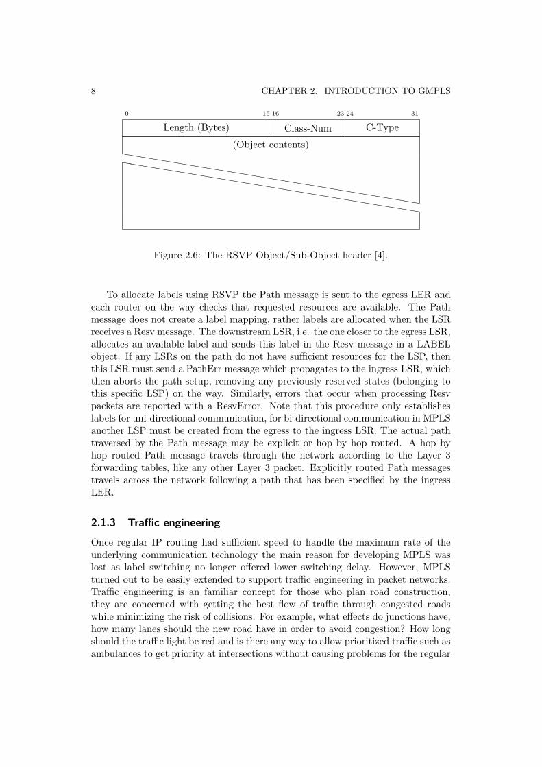
All RSVP packets share a common header, followed by a number of Type-Length-Value (TLV) fields called objects which may have additional TLV field within(these are called sub-objects). The TLV fields are actually in the Length-Type-Valueorder1 with the Type field split into two separate field, the Class field and the C-Type field. The common header carries the type of the message, total length ofthe message, and information for defragmentation (see figure 2.5). Any additionalinformation is carried in objects or sub-objects (see figure 2.6).

1I will refer to them as TLVs or objects despite this order of the fields.


0 15 16 23 24 31

Length (Bytes) Class-Num C-Type

(Object contents)hhhhhhhhhhhhhhhhhhhhhhhhhhhhhhhhh

hhhhhhhhhhhhhhhhhhhhhhhhhhhhhhhhh

Figure 2.6: The RSVP Object/Sub-Object header [4].

To allocate labels using RSVP the Path message is sent to the egress LER andeach router on the way checks that requested resources are available. The Pathmessage does not create a label mapping, rather labels are allocated when the LSRreceives a Resv message. The downstream LSR, i.e. the one closer to the egress LSR,allocates an available label and sends this label in the Resv message in a LABELobject. If any LSRs on the path do not have sufficient resources for the LSP, thenthis LSR must send a PathErr message which propagates to the ingress LSR, whichthen aborts the path setup, removing any previously reserved states (belonging tothis specific LSP) on the way. Similarly, errors that occur when processing Resvpackets are reported with a ResvError. Note that this procedure only establisheslabels for uni-directional communication, for bi-directional communication in MPLSanother LSP must be created from the egress to the ingress LSR. The actual pathtraversed by the Path message may be explicit or hop by hop routed. A hop byhop routed Path message travels through the network according to the Layer 3forwarding tables, like any other Layer 3 packet. Explicitly routed Path messagestravels across the network following a path that has been specified by the ingressLER.

2.1.3 Traffic engineering

Once regular IP routing had sufficient speed to handle the maximum rate of theunderlying communication technology the main reason for developing MPLS waslost as label switching no longer offered lower switching delay. However, MPLSturned out to be easily extended to support traffic engineering in packet networks.Traffic engineering is an familiar concept for those who plan road construction,they are concerned with getting the best flow of traffic through congested roadswhile minimizing the risk of collisions. For example, what effects do junctions have,how many lanes should the new road have in order to avoid congestion? How longshould the traffic light be red and is there any way to allow prioritized traffic such asambulances to get priority at intersections without causing problems for the regular


traffic?If one imagines data packets as cars, network links as roads, and switches and

routers as road junctions the same issues more or less apply to traffic engineeringin packet networks. Congestion on roads causes delays and accidents, in packetnetworks it causes delays and packet loss. IP networks are generally Shortest PathFirst routed – which is a great scheme as long as the network is unused, packets reachtheir destination quickly while using the minimum amount of network resourcespossible (assuming that all links have basically the same cost – thus the goal is tominimize the number of hops). However, if the network has got a lot of traffic goingthrough it the shortest path may become congested and routers will start to dropthe packets they cannot forward. Even if there are routes that avoid the congestedrouters, traffic will still be routed over the shortest path leaving alternative pathsunderutilized. There are ways to manage congestion, for example DiffServ or IntServcan be used to prioritize traffic so that it is not dropped and TCP has mechanismsfor lowering transmission rates when congestion is detected [5][6][7]. These are goodfor improving the reliability and quality of traffic delivery, but do not increase theamount of traffic which can go from one point to another in an Shortest Path Firstnetwork [8].

In order to increase the amount of traffic the network can deliver some partsof the traffic has to be delivered via these alternate paths. Equal-cost multi-pathrouting is another routing scheme which under some circumstances is able to makeuse of these alternate paths. When an Shortest Path First router calculates routesand is confronted with more than one path to a destination with the same length orcost it chooses one of them, equal-cost multi-path instead stores both paths. It canthen choose to either use an alternative path when the first one becomes congestedor to load balance the different paths. The road analogy for this would be twoparallel roads of the same lengths to a destination. The second road would eitherbe opened when the first becomes congested or one would direct every other cardown the second road. However, if these equal-cost paths converge at one pointand the congestion occurs on a link further down the parallelism might not makea difference. The problem of not using alternate paths still exists as well, a pathwhich costs one unit more would not be used with equal-cost multi-path.

Better traffic engineering can be achieved if one knows all the paths and linksof the network and the current utilization of them and then somehow directs trafficbased on that information. And here is where MPLS has found a niche, if oneextends it to support an explicit route instead of only a Shortest Path First route itcan be used to direct traffic over predetermined links chosen for traffic engineeringreasons. By extending the MPLS routing protocols to carry information such as theavailable bandwidth of links and extending signaling protocols to create an LSP onan explicit path one can support advanced traffic engineering. These extensions ofthe original MPLS protocols are called MPLS TE [9].


2.2 Generalized MPLS

The origin of GMPLS was a wish to automate previously manual systems forprovisioning services in transport networks. The manual planning and configurationof the services could take a long time and negatively affect other services [10].As networks grew in size the demand for an automated way to deal with thisgrew. As optical networks became more popular, ways to deal specifically withlambda switching networks (see section 3.1.2) was developed. It was realized thatdistributing label mappings {incoming label, outgoing label} and lambda mappings{incoming lambda, outgoing lambda} was essentially the same problem and couldutilize a similar solution. One proposal which borrowed heavily from MPLS wascalled Multi-protocol Lambda Switching (MPλS), however it never became anofficial standard [11].

The generalization of MPLS was expanded to include switching time slots inTDM systems, switching between optical fibers, and switching layer 2 frames –as these are more or less the same thing. Why not create a unified standardfor managing all these technologies since they were essentially the same problem?Another advantage of creating a general protocol it that networks of different typescan now interoperate easily. That means that end-to-end services could be set upand maintained over networks composed of different networking technology withoutany complicated interoperability layers. The ability to distribute traffic engineeringinformation between technologies may also lead to more efficient provisioning ofservices, for example if there is a problem within one segment this can be taken intoaccount before any signaling is performed. Larger networks also lead to a largeramount of routing traffic, hence GMPLS can be deployed in several models whichbalance control plane overhead against TE efficiency (see section 2.2.6 for more onthis).

The effort needed to calculate paths grows with the number of nodes involvedand is likely to be slower when performed for many different kinds of technologiesat once – due to different constraints on each of the different technologies. Pathcalculation is only necessary when initially provisioning the service so this maynot be a large problem, however if many paths fail simultaneously this could bea problem since many new routes would be requested at once. This could bemitigated by pre-calculating failure paths, perhaps completely disjoint from theoriginal path. If the original path fails one of the pre-calculated alternatives can besignalled without any need for additional calculation. The task of performing routecalculation, which may be computationally expensive, can either be centralized ordistributed or somewhere in between, this is discussed in section 2.2.10.

2.2.1 Control and Data plane

The nature of some of the technologies intended to be used with GMPLS requiresthat the control plane and data plane must be separated. In packet switchingsystems control data can be sent over the same channels as traffic, as routers and

2.2. GENERALIZED MPLS 11

In-band control Out-band control

Data traffic

Control traffic

Figure 2.7: Example of in-band and out-band control. Data traffic (shown as adashed line) and control traffic (shown as a filled line - above the data traffic) goingthrough packet routers and splitting up when going over optical network componentsconnected to packet routers.

switches read the header of each packet and if a packet is found to be destined toitself it can pass it along to the control system within, this is called in-band control.This is not possible for some devices (e.g. optical switches, see section 3.1.2) sincethey do not examine the data that they transport, therefore control data must becommunicated through a separate control channel (see figure 2.7), this is calledout-band control. In WDM systems this can be done either by having a separateconnection, for example an Ethernet link connected to the switch or, if the switchsupports it, a data channel reserved for control data.

Separating control and data plane also adds resilience to the network, the dataplane can continue to function even if the control plane is broken (although no newconnections can be made) and vice versa. However, detecting errors in the dataplane may be harder since you cannot detect errors by loss of control traffic as innetworks with in-band control data. Errors such as “loss of light” in some opticalnetworks can only be detected at the end of the light path and thus finding the faultylink or device may not be a trivial task. To aid this process the Link ManagementProtocol (LMP) and LMP-WDM for optical systems may be used which are coveredbriefly in section 2.2.9. The Link Management Protocol helps the switch to discoverits links and their capabilities, as well as assisting in the detection and isolation oferrors on the links.

2.2.2 Interface Switching Type

Five kinds of interface switching types have been defined: Packet switching capable(PSC), Layer 2 switching capable (L2SC), Time division switching capable (TDM),Lambda switching capable (LSC), and Fiber switching capable (FSC). The valuesused to represent these switching types in the signaling and routing protocols canbe seen in table 2.1, how they are used is described in sections 3.3.4 and 2.2.8. Anetwork interface on a node is said to have a Interface Switching Capability (ISC)


Table 2.1: Interface Switching Types and their corresponding values

Switching type ValuePSC-1 1PSC-2 2PSC-3 3PSC-4 4L2SC 51TDM 100LSC 150FSC 200

depending on what information the node can use to switch data that arrives onthat interface. For example if data arriving on an interface can be switched basedon a Layer 2 header, such as an Ethernet frame header, then that interface is L2SCcapable. If the interface can separate different colors of light from an optical fiberand the node can direct them into different optical fibers, then the interface is oftype LSC. If the interface can switch packets based on an MPLS label, it is oftype PSC and so on. The four different PSC types can be used with MPLS labelstacking to tunnel LSPs within LSPs (see section 2.1.1)[12]. All interfaces on a nodedo not have to have the same switching type. Additionally an interface may actuallyhave several switching types. For example an interface may be able to switch onboth an MPLS label and a Ethernet header, then it would then be both PSC andL2SC capable. Nodes that have interfaces which support multiple switching types(per interface) are called ”hybrid” nodes whereas those with only a single switchingtype per interface are called ”plain” or ”simplex” nodes [13]. Hybrid nodes are notconsidered in this thesis.

2.2.3 Regions and Layers

There is some confusion regarding the nomenclature surrounding GMPLS, the termsregion and layer need to be clarified. In this thesis the terms will be used as they aredefined in RFC 4397 which defines a layer as “a set of [data plane] resources of thesame type that could be used for establishing a connection or used for connectionlessdata delivery.” [14]. Using this definition a multi-layer data plane device could forexample be an Ethernet interface capable of sending in 100 Mbit/s as well as 1Gbit/s. A “TE region” is defined as “a set of one or more layers that are associatedwith the same type of data plane technology”, such as MPLS, ATM, WDM, etc.The term “TE region”, “LSP region”, and just “region” can be used interchangeably.Multi-layer networks are not considered in this thesis; we will instead only focuson multi-region networks where each region consists of only a single layer. For anexample of a multi-region GMPLS network see figure 2.8.


Figure 2.8: Multi-region network with three regions, LSC, L2SC, and PSC.

2.2.4 Labels

In MPLS labels describe a Forward Equivalence Class; this is also true in GMPLS,but a label may also describe a physical resource, for example a wavelength or a timeslot. When the labels describe a physical resource the label is often not actuallycarried with the data (as for example an MPLS shim label or Ethernet label).Instead the label only exists in the control plane where it describes how the switchingmatrix of the particular switch should be set up. In that case the label may bereferred to as a ”virtual” label. The need to support different switching techniquesmeans that the label format has to be generalized in order to fit the switchingcapability and encodings used by different switches (e.g. ATM and Ethernet areboth L2SC, but need different label formats since they switch on different kindsof headers). The collection of these specific label formats are called “generalizedlabels”, and each of them has to contain the information necessary for the specifictechnology to control its cross-connect in order to create a path. As in MPLS thelabels may be link-local, but in some networks (e.g. WDM, Ethernet) the samelabel may have to be used through the whole network segment (so called end-to-endlabels). The generalized label itself is has a variable length; in most cases it is a32-bit value, but longer labels are supported. Shorter labels such as MPLS or FrameRelay labels are right justified within a 32-bit value [15].

The different generalized labels have no field to indicate what type of label itcontains, therefore one cannot easily conclude how to interpret a label. Findingout how to interpret a generalized label requires information about the TE-link towhich the label should be allocated. By examining the Switching Capability of the


far- and near-end of the TE-link one can determine the label type in some cases. Inother cases the Encoding taken either from the Traffic Engineering Database (seesection 2.2.8) or the Label Request (see section 2.2.7) might be necessary. If forexample the switching capabilities of the TE-link are [PSC, PSC] the label is anMPLS label; if the switching capabilities are [PSC, LSC], then the label indicates alambda [12].

2.2.5 Interface IdentificationThe data plane consists of links between data interfaces, which may have differentcapabilities (such as a switching capability, adaption capability, and terminationcapability). These different capabilities and other constraints (such as availablebandwidth) are taken into account when calculating a path. When signaling anLSP these interfaces have to be identified in some way in the Explicit Route Object(ERO) of the RSVP Path message (see section 2.2.7), this identification can beeither numbered or unnumbered. A numbered interface has a public or private IPaddress assigned to it, this IP address can then be used to unambiguously identifythe link in RSVP-TE and OSPF-TE. However, for other interfaces, such as Ethernetor WDM interfaces that cannot terminate traffic, assigning an IP address to identifythe interface may be a waste of IP address space (if the addresses are public) andassigning this interface an IP address makes little sense if it cannot receive IP traffic.When assigning private IP addresses to you need to keep track of all the addressessince they have to be unique within the network, this is error prone and may requiresa significant amount of work. Instead of assigning IP addresses one can use so calledunnumbered identifiers. The unnumbered identifier consists of the LSR’s Router ID(which usually is a network unique loop back IPv4 or IPv6 address, in order tobe reachable through any of its interfaces) combined with a node-unique 32-bitidentifier. This combination is a network unique identifier that can be generatedby any node without the need for some kind of address management scheme. Onecan imagine other identifiers that could be used, for example MAC addresses whichare already used by some networking technologies. However, adding technologyspecific identifiers complicates the protocols and implementations, especially whenthere already are generic identifiers defined.

2.2.6 Network ArchitectureGMPLS can be deployed in three distinct architectural models:

• The peer or unified service model

• The overlay or domain service model

• The hybrid or augmented model

The models primarily differ in how much information is distributed betweendomains and how services are set up. In the peer model all LSRs in the network


IP Network

GMPLS Access Network

GMPLS CoreNetwork

MPLS Network

End-to-end service

Figure 2.9: The peer model. A common control plane is used to route and signal apath across a network of different technologies and realize an end-to-end service.

have full visibility of the entire GMPLS network, each node knows the completetopology of the network and what resources are available (see figure 2.9). A singlecommon signaling protocol is used through the network which allows clients at theborder to set up end-to-end services. However, this model has scaling problems asthe number of nodes grow, but it is also the most flexible model in terms of serviceestablishment since a full view of the network is kept and paths are fully trafficengineered end-to-end.In the overlay model (see figure 2.10) each LSR has a limited visibility – eitherto the network it is a part of (i.e. with the same switching capability) or toits administrative domain. This means that no TE information is shared witha neighbor of either a different technology (e.g. between MPLS and Ethernetswitched networks) or of a different administrator (e.g. between two InternetService Providers). Instead a User-to-Network Interface (UNI) is placed at theborder of network domains, there the client network asks the interface for serviceand the ”server” network is free to deliver the service in its own fashion. Thisallows for greater separation of networks which are free to operate independentlyof each other. In this approach service providers can operate their own networkwithout allowing any routing information or signaling from partners or competitorsinto their own control plane and similarly not permitting any of their routing orsignaling information to leave their network. Several protocols for communicatingvia a UNI have been developed, for example the Optical Internetworking Forum’sUNI implementation which sends the service request as a new RSVP-TE object.This model scales better but obviously paths cannot be fully traffic engineeredsince each network performs setup on its own.

The hybrid model is a mixture of the above models (see figure 2.11). It allows forsome trust between network domains and a bit of leakage of routing and signalinginformation between domains, but not the full topology. This removes the need forextra protocols such as UNI, as all domains can utilize GMPLS. Depending on howmuch information is shared over domain borders path setup may be fully or almost


End-to-end service in higher-layer network

User-to-NetworkInterface

Locally realizedservice

Figure 2.10: The overlay model. ”Client” or ”higher layer” networks request servicesfrom another network in order to create an end-to-end service. No signaling orrouting information is shared between the networks.

Figure 2.11: View of the network from nodes in the leftmost network segment inthe hybrid model. Signaling is handled in the same fashion as in the peer model.

fully traffic engineered.This model is similar to the way the Internet is designed, typically each

autonomous system runs an inter gateway routing protocol (IGP) and a exteriorgateway routing protocol (EGP). The IGP handles routing internally in theautonomous system, but exchanges some information with the EGP that isresponsible for routing between the autonomous systems.

In the rest of this thesis only the peer model will be considered since it is thesimplest model, it avoids the need for UNI protocols, and does not need to restrictcontrol plane information at borders.

2.2.7 Signaling Extensions

RSVP-TE is the primary signaling protocol used in GMPLS. (The IETF stoppeddevelopment of CR-LDP, thus it is unlikely that it will be extended to supportGMPLS.) Many of the features of RSVP are reused in RSVP-TE, but someextensions have been made to support label distribution, explicit routing, differentdata plane network technologies, separation of control and data plane, and more.A number of these signaling extensions were introduced when creating MPLS TE,these are kept or updated by GMPLS which also introduces several extensions of


0 7 8 15 16 23 24 31

Length Class-Num (19) C-Type (4)

LSP Enc. Type Switching Type G-PID

Figure 2.12: The Generalized Label Request object, request a label for specific typeof LSP while informing the egress what kind of traffic it will carry [15]

.

its own. Some of the more important extensions are presented here in the form inwhich they appear within GMPLS.

• Label management

– Generalized Label Request– Suggested Label– Upstream Label

• Explicit routing

– Explicit Route Object– Record Route Object

• Control and data plane separation

– Extended HOP Object

Label Management

By adding a Label Request object to a RSVP Path message the sending node canrequest that the downstream node return a label which can be used to send trafficto the downstream node. The Label Request object carries three fields: encoding,switching type, and Generalized Payload Identifier (G-PID) (see figure 2.12). Theencoding field describes how data traffic will be presented to the transport mediumand determines what type of LSP is created. For example an encoding of ”Packet”would request an MPLS label (and MPLS data plane reservation). The switchingcapability field is useful if the LSR is a so called hybrid node, i.e. it can switch onmultiple switching type levels. For example an optical switch can be both LSC andFSC at the same time – if it is capable to not only switch individual wavelengthsbut also switch between different fibers. In that case it may be necessary to specifyon what level the switching should take place. The G-PID indicates to the egressnode what type of payload is carried within the LSP. The G-PID can use regularEtherType values, but some additional values have been specifically defined forGMPLS (such as SONET/SDH and HDLC traffic) [15].

In MPLS labels are returned in the RSVP Resv message which makes the LSPsuni-directional, but GMPLS uses by default bi-directional LSPs. Instead of having


to setup two separate LSPs to achieve bi-directional communication (as in MPLS)GMPLS can send labels downstream in the RSVP Path message in order to establisha two-way label mapping during a single Path setup. This label is carried in theUpstream Label object which has the same properties as the regular Resv Labelobject, i.e. it can be swapped at each hop, carry the same types of labels, etc.The use of the Upstream Label object reduces both the signaling overhead andthe time needed to create LSPs, since only one reservation request is necessary.Another label carrying object is the Suggested label object. This object can be sentwithin a Path message to indicate what label the upstream node would like to use.Using the suggested label object can also reduce LSP setup time as it can be usedwith a pre-configured data plane (i.e., the configuration is done before the actualreservation is made) when a Resv message is received. In many switches the timeto create a switching rule is negligible, but in (for example) some optical switcheswhich need to move physical components this many increase the overall LSP setuptime significantly.

Explicit Routing

To support explicitly routed LSPs the Explicit Route Object (ERO) has been added.This object holds a list of ”abstract nodes” which should be traversed by the LSP(see figure 2.13). There are three different abstract node types defined: IPv4, IPv6prefix, and Autonomous System (AS) number subobject. Each of these abstractnodes can contain several real nodes. For example the AS subobject contains allthe GMPLS nodes within an Autonomous System, an IPv4 subobject contains allthe GMPLS nodes within a specific subnet (for example a /24 subnet or a singlehost if the subnet prefix is /32). By creating a list of these objects an explicit routecan be specified with large flexibility in granularity.

Each abstract node is defined as either ”strict” or ”loose”. This ”strictness”and ”looseness” is always relative to the previous abstract node, if a node is strictthe path traversed must consist of nodes which are part of the previous and thestrict abstract node. When traversing the previous abstract node in conjunctionwith a loose hop the path may traverse nodes which are not part of either abstractnode. Note that this does not mean that all the nodes specified in a strict abstractnode has to be traversed, it is not necessary to traverse all the nodes in an AS forexample, only the ones needed to reach the following abstract node.

While traversing the nodes specified in the ERO in the Path message the nodesare successively removed from the ERO. When the egress node is reached it has noway to know what path was used to reach it (except the previous hop). In order tocollect this information the Record Route Object contains a list of abstract nodes.The abstract nodes used in the Record Route Object is identical to the ones usedin the ERO with the exception of that the AS number subobject is not allowedwhile a Label subobject can be used to record what label was used on a specificlink. By adding abstract nodes (and optionally the label used) to this list as thePath message traverses the network both ingress and egress node may find out the


0 1 7 8 15

L Type Length

(Subobject contents)hhhhhhhhhhhhhhhhh

hhhhhhhhhhhhhhhhh

0 7 8 15

IPv4 AddressIPv4 Address (cont)

Prefix Length Reserved

Figure 2.13: Abstract node (left) and IPv4 subobjects (right). The L flag indicatesof the hop is loose or strict. The Type field holds the type of the subobject (IPv4or IPv6 prefix, AS number). The IPv4 subobject contains an IPv4 address andnetmask (prefix length) [16]. (Note that the widths of these figures are 16 bits.)

exact path used (as the egress is allowed to send the Record Route Object back tothe ingress in the Resv message)[16].

Control and data plane separation

When an LSR receives an Path message it stores some information about it in a socalled Path State Block. The Path State Block contains, for example, informationabout the previous hop. This information is taken from the RSVP_HOP objectcarried in the Path message. Before GMPLS the RSVP_HOP contained only anIPv4 or IPv6 address and a Logical Interface Handle (a node local value identifyingthe interface used to send the RSVP message) which was used by the LSR tofind out whom to send replies to. The previously stored RSVP_HOP object isreturned within the Resv message to make it easier for the previous hop to findout which interface it used to send the Path message. The previous node cannotassume that the Path message was sent on the same interface that receives the Resvmessage, since the message may pass through a network between these two nodes(which is why this information is sent along with the messages). Since GMPLSsupports out-of-band signaling – and multiple data plane links per control plane link– the RSVP_HOP object has been extended to indicate which data plane interfacethe message refers to as well as the control plane interface. There are two newRSVP_HOP objects which contains either an IPv4 or IPv6 control plane addressand a Logical Interface Handle and a TLV identifying the data plane interface (seefigure 2.14). There are five types of data plane interface identifier TLVs: IPv4, IPv6,unnumbered interface, and two component interface identifiers which are identicalto the unnumbered interface TLV except for the Type field.

2.2.8 IGP Extensions

As previously stated GMPLS can use both ISIS-TE and OSPF-TE for routing of thecontrol plane and dissemination of TE information in the network. I will however


0 15 16 23 24 31


IPv4 Next/Previous Hop Address

Logical Interface Handle

Type (3) Length (12)

IP Address

Interface ID

TLV

Figure 2.14: An IF_ID RSVP_HOP object with an IPv4 control plane identifierand a unnumbered interface data plane identifier [15] [17].

0 7 8 15 16 31

Version # Type Packet length

Router ID

Area ID

Checksum AuType

Authentication

Authentication

Figure 2.15: The OSPF packet header. The version field indicates what OSPFversion is used, the Type field differentiates the different messages types, and thePacket length is the length of the entire packet in bytes. Router ID is the ID ofthe source of the packet. The AuType and Authentication fields can be used toauthentication the packet [19].

focus on the extensions to OSPF which enables this.OSPF was designed to be used within an autonomous system. The networks in

an AS can be subdivided into areas making routing more efficient [18]. The areas areconnected by area border routers which summarize the routing information aboutan area and send it into other areas. A OSPF network contains at least one area,the backbone area. OSPF has five different kinds of messages, all with a commonheader (see figure 2.15) [19]. These five messages are Hello, Database Description,Link State Request, Link State Update, and Link State Acknowledge (see table 2.2for details).

Some of these message can carry a list of Link State Advertisements (LSAs)or a list of LSA headers. Most important is the Link State Update message whichperforms the actual flooding of link state information in the network by distributingLSAs. In OSPFv2 there are five kinds of LSAs which describe the local topology


0 15 16 31

LS age Options LS Type

Link State IDAdvertising Router

LS sequence number

LS checksum length

Figure 2.16: The common LSA header [19].

of the router transmitting them (see table 2.3). For example, a router originates arouter-LSA which contains a list of all its links, whether the link is a point-to-pointlink to another router, a link to a network without any other routers, or any of theother four types of links that exist in OSPFv2. If a router is the Designated Routerfor a network segment (either by being the only router on the segment or by election)it transmits a network-LSA which describes all routers attached to that particularnetwork segment. The other LSA types announce links across areas (SummaryLink), links that reach AS border nodes (Summary Link to AS Boundary Router),and links received from other routing processes such as BGP (External LSA). AllLSAs share a common header and are distinguished from each other by a 8-bit value(see figure 2.16). The header contains several fields, the LS age field is a timer whichholds the age of the LSA in seconds, updated by each router. The Options fieldcontains some flags, for example it can indicate if the area is a stub area or not. LStype is the type field which is shown in table 2.3. The Link State ID field holds anidentifier for the link which this LSA concerns, for example the router IP address ina router LSA. The Advertising router field holds the Router ID of the originator ofthe message. The LS sequence number field is a sequence number assigned to eachLS Update message. The length field is the length of the whole packet in bytes.

All routers within an area receive and store the router- and networks-LSAsfrom that area in a Link State Database. After the Link State Database has beenconstructed it is used to calculate Shortest Path First routing tables.

The ”OSPF Opaque LSA Option” is an additional three LSA types which makesit easy to extend OSPF for application specific purposes [20]. These LSAs areflooded like the other LSAs, but are not used for regular OSPF routing, insteadthey carry application specific data. Of importance to us, these are the LSAs2

used to carry TE information in GMPLS [21]. The TE LSAs have a standard LSAheader followed by a Type-Length-Value field to distinguish between the differentTE objects. The TE LSA TLV contains a number of sub-TLVs which hold theactual TE link information, such as Link ID, remote and local addresses, reservablebandwidth, etc. An actual LS Update message may look like the one in figure 2.17where the OSPF header can be seen along with three different LSA headers, the

2Actually only the area local opaque (type 10) LSA is used


Table 2.2: OSPF message types.

Type Name Description1 Hello Sent periodically on all interfaces to create and

maintain routing adjacencies2 Database Description Sent when an adjacency is created in order to

exchange information about the LSAs in therouter’s database

3 Link State Request Used to request fresh information if part of therouter’s database is out-of-date

4 Link State Update Performs the actual flooding of LSAs toneighbors, multicasted if the network supportsit

5 Link State Acknowledge Sent to acknowledge Link State Updates in orderto make the flooding reliable

Table 2.3: Different LSAs, their use and flooding scope.

Type Name Scope Description1 Router Area local Describes all links of a particular

router2 Network Area local Describes all routers in a network3 Summary Inter-area Summarizes the links in one area

and informs the other attachedareas

4 ASBR-Summary AS (except stubs) Informs areas which networks areattached to AS border nodes

5 External AS (except stubs) Informs areas of routes receivedfrom external routing processes,such as BGP

9 Link local opaque Link local Carries opaque informationwithin one network

10 Area local opaque Area local Carries opaque informationwithin one area

11 External opaque AS (except stubs) Carries opaque informationwithin one AS


OSPF header, Type 4 (Update)

Number of LSAs: 3

LSA header, Type 1

Router LSA header, links: X

X links

LSA header, Type 2

Network LSA header

Attached routers

LSA header, Type 10, length: Y

Type 2 (Link info) Length: Z

Sub-TLV Type 2 (Link ID) Length: 4

Link ID: A.B.C.DSub-TLV Type 6 (Bandwidth) Length: 4

Bandwidth: X bytes/s

Sub-TLV Type ...

TE

LSASub-T

LVs

Figure 2.17: Simplified illustration of how an OSPF LS Update message may beconstructed. This one carries three LSAs, one router LSA, one network LSA, anda TE LSA. The TE LSA is in turn composed of one TLV consisting of several sub-TLVs which holds information such as Link ID, Maximum reservable bandwidth,Interface Switching Capability Descriptor and so on.

TE LSA TLV and sub-TLVs are also shown. Unlike the regular LSAs the TE LSAsare not stored in the Link State Database, but in a separate Traffic EngineeringDatabase.

2.2.9 Link Management Protocol

The Link Management Protocol (LMP) is responsible for data plane link discovery,configuration, and fault isolation. This could partly be done manually, at least theconfiguration of data plane links could be done, but with a large number of links this


becomes error prone and can be quite a lot of work to both initially configure andkeep up to date. The LMP protocol is UDP based and runs on port 701 betweenGMPLS nodes. The messages are similar to the RSVP-TE message with a commonmessage header followed by objects and sub-objects (TLVs) distinguished by Classand C-Type. The main functions of LMP are:

Control channel management Initialization and management of control chan-nels. Initially data plane neighbors establish each others identity andcapabilities, after this is done they enter a management phase whichperiodically sends Hello messages to make sure there is still connectivity.

Data plane link discovery Discovery of and connectivity check are needed oneach of the data plane links to and from neighbors. Before this is done thenode only knows the local identifier of each link, but not the state of or theremote identifier of each link.

Data plane link capability exchange Depending on data plane technology anexchange of link information may follow link discovery. This may also benecessary if multiple types of links are supported.

Data plane link verification Verification can be conducted at any time to checkconnectivity and the status of a data plane link. The procedures followed toverify a link are identical to the link discovery procedures.

Fault isolation One of the most important parts of LMP is fault isolation. It isinitialized by a downstream node whenever a fault such as signal degradationis noticed. Since some data plane technologies are oblivious to the data theyare transporting another protocol is sometimes necessary to find the faultylink in order to bypass it.

Authentication LMP has support for authentication, although it is not arequirement it may be a good idea to use authentication. Since the controllink or channel can traverse a public IP network each message should beauthenticated in order to prevent spoofing attacks.

An extended LMP protocol is LMP-WDM which runs between a OXC (seesection 3.1.2) and optical components which may be external to the OXC, such asoptical amplifiers and multiplexers. These external components are known as anOptical Line System.

2.2.10 Path Computation Element

The Path Computation Element is responsible for performing path calculationwithin the GMPLS network. Since path calculation is usually only necessary atthe edge of the network, there is no requirement that each node in the networkcan perform path calculation, unlike for example IP networks (where each routes is


expected to be able to perform route calculation). Instead the LSRs implement aprotocol that can send requests to the Path Calculation Element which calculatesa route and returns it to the LSR. This client-server path calculation architecturemakes it possible to make path calculation fully decentralized, centralized, or variousdegrees thereof. This is useful since constraint-based path calculation may be acomputationally expensive operation, if it is centralized the LSRs can be ”dumber”and cheaper to produce. Multiple Path Calculation Elements can be used to makethe path calculation more resilient and route request can be distributed betweenthe Path Calculation Elements in order to balance load.

Chapter 3

Multi-region GMPLS Networks

Many complicated and interesting issues in GMPLS networks arise when going fromone network region to another. Path calculation has to take into account constraintsspecific to each region; additionally extra signaling may be necessary to tunnelswitching types and a correct “inter-technology” mapping must be established. Thefocus of this thesis is the switch between L2SC and LSC regions, specifically betweenEthernet and a Wavelength Division Multiplexing system. How these differentswitching systems operate is discussed below.

3.1 Network Technologies Considered in this Thesis

3.1.1 EthernetEthernet has been a very popular network technology since it was invented in themid-1970s. It is standardized by the Institute of Electrical and Electronics Engineers(IEEE) in the IEEE 802.3 family of standards [22]. Traditionally Ethernet has beenused in Local Area Networks (LANs). In recent years Ethernet has also been used toimplement Metropolitan Area Networks and carrier backbone networks, displacinglegacy time division multiplexing systems such as synchronous optical networks(SONET/SDH). Metropolitan and carrier networks frequently use 1 or 10 GigabitEthernet; as the physical layer supports both short twisted-pair cables and longeroptical fibers. A major reason for the popularity of Ethernet is the relative lowprice of Ethernet equipment due to the large production volume [23].

The Ethernet frame header contains two addresses, a source and destinationMedia Access Control (MAC) address. When a switch receives a Ethernet framethe destination MAC address is examined and a table look-up indicates on whichport the frame should be forwarded; this is based upon an earlier procedure called”learning” which has discovered the MAC addresses of Ethernet interfaces attachedto the different ports. If the destination MAC address is not found in the forwardingtable, i.e. the destination address is unknown, the frame is transmitted on all portsexcept for the one it arrived on. Each port of a Ethernet switch belongs to adifferent collision domain, every node in a collision domain can intercept frames

26

3.1. NETWORK TECHNOLOGIES CONSIDERED IN THIS THESIS 27

Figure 3.1: Ethernet Type II frame format. The header contains source anddestination address and a field indicating what type of data is carried in the payload.The frame check sequence (FCS) is a checksum of the frame inserted after thepayload.

Figure 3.2: Example of two connected Ethernet switches, each with 2 VLANs.Equipment on a VLAN can only communicate with equipment on the same VLAN.

sent on that domain and if they try to send frames at the same time the frameswill collide. Another important domain is the broadcast domain, this is the setof collision domains reached by sending a local broadcast frame (a frame with thedestination MAC address ff:ff:ff:ff:ff:ff). The broadcast domain generally covers allcollision domains on a bridged network, but does not extend past network layerrouters. Several slightly different Ethernet frame formats exists, see figure 3.1 forthe format of the common Ethernet Type II frame. The two byte EtherType fieldindicates what type of data is carried in the Payload (for example the value 080016represents IP traffic, 080616 ARP, etc). The four byte Frame Check Sequence (FCS)is a checksum used to detect corrupted frames.

Sometimes it can be useful to create different broadcast domains on top of aphysical network in order to create logical network topologies different from thatof the physical network. This can be done on Ethernet networks by using VirtualLANs (VLANs). Using VLANs one can partition different ports on a switch to bepart of different networks.

The example shown in figure 3.2 shows two connected switches with two VLANseach. Interfaces on VLAN 1 can communicate with interfaces on the same VLANon both switches, but not with interfaces connected to VLAN 2.

VLANs were implemented on Ethernet following the IEEE 802.1Q standardwhich adds a tag after the source MAC address in the Ethernet header. In figure3.3 an Ethernet Type II frame with a 802.1Q VLAN tag is shown in which one can

28 CHAPTER 3. MULTI-REGION GMPLS NETWORKS

Figure 3.3: Ethernet Type II frame tagged with 802.1Q VLAN Tag.

Figure 3.4: End-to-end Ethernet label using VID and destination MAC address.

see the VLAN tag inserted between the source address and the EtherType field. TheVLAN tag consists of two parts: the Tag Protocol Identifier (TPID) and the TagControl Information (TCI). The TPID takes the previous position of the EtherTypefield and is set to the value 810016 and informs the switch that the frame is tagged,the actual EtherType is placed after the TCI. The 2 byte TCI is divided into a3-bit field for priority, a 1-bit field called Canonical Format Indicator (CFI), and a12-bit field for the VLAN identifier (VID) [24]. The priority field can be used towith IEEE 802.1p (part of IEEE 802.1D since 1998) to provide link layer Quality ofService. The CFI field is used to provide interoperability with Token Ring networks,on Ethernet networks it is always set to zero. The 12-bit VID identifies what VLANthe frame belongs to. The VID could be used as a GMPLS label in the same wayMPLS labels are used, with swapping at each LSR. Unfortunately, this violates the802.1Q standard and is not supported by Ethernet switches. If the VID is used asa label we are forced to use it as an end-to-end label, meaning that the same labelis used for each hop along the entire Ethernet segment of the path. This constraintlimits the number of LSPs to 4093 (12 bits minus 3 reserved labels) per link andEthernet segment. By using the VID in combination with the destination addressof the egress as the label; LSPs can share VIDs and the limitation changes to 4093LSPs per destination address, quite an improvement (see figure 3.4).

Other possibilities for a GMPLS Ethernet labels can be found in the IEEE802.1ad (Provider bridge [25]) and IEEE 802.1ah (Provider Backbone Bridges [26])standards. These two standards allow provider networks to transport VLAN taggedEthernet traffic, which makes it possible to create for example link layer privatenetworks (virtual private LAN services). IEEE 802.1ad (also known as Q-in-Q) isan amendment to the 802.1Q VLAN tags which adds another almost identical VLAN


tag in addition to the original one. These so called Service Tags may be a betterchoice for GMPLS labels since it would allow the GMPLS network to transportEthernet frames which are already tagged (perhaps for use in a customer’s network).The other possibility is using IEEE 802.1ah which adds additional MAC addressfields as well as an additional VID. At the time of writing neither the GMPLS labelformat or which of these available tags to use has been standardized. Work on thisis being done in the IETF Common Control and Measurement Plane (CCAMP)work group [27].

3.1.2 Optical NetworksWavelength Division Multiplexing (WDM) is very similar to the Frequency DivisionMultiplexing (FDM) that is used in systems operating in the lower frequencies ofthe electromagnetic domain. The bandwidth of a channel is split into multiplediscrete channels, in WDM the sub-channels are commonly referred to as lambdas,from the Greek letter λ used in physics to denote wavelength. In WDM the mediatypically is an optical fiber instead of open air. The bandwidth frequently rangesfrom the infra-red to ultraviolet - as this frequency range has low attenuation withinthat fiber, due to the materials used and the design of the fiber. Depending on thedifference between the frequencies of the different lambdas (the so called channelspacing) the technique is called either Coarse Wavelength Division Multiplexing(CWDM) or Dense Wavelength Division Multiplexing (DWDM). Typical channelspacing for CDWM signals is 2500 GHz and in DWDM between 12.5 and 100 GHz(see table 3.1).

Table 3.1: Values used in the Grid field and in the Channel Spacing (C.S.) field.

Grid ValueITU-T DWDM 1ITU-T CWDM 2

Future use 3 - 7

C.S.(GHz) Value12.5 125 250 3100 4

Future use 5 - 15

Components of Optical Networks

In order to switch optical signals there are two basic approaches: optical-electronic-optical and the optical-optical-optical. In optical-electrical-optical the optical signalis demuxed and converted into an electric signal. An advantage of this approachis that an electrical signal can be switched easily and regenerated at perhaps adifferent wavelength than the incoming signal and emitted into a different fiber. Adisadvantage of optical-electrical-optical is that the optical signal has to be decodedand sent through an electronic switching fabric, limiting the device to specific signalencodings and data rates. In the optical-optical-optical case the incoming signal is


Drop Add

Trunk Trunk

Add/Drop

Trunk Trunk

Add/Drop

Figure 3.5: 1st and 2nd degree OADM.

demuxed (if necessary) and sent through a optical switching fabric. Such an opticalswitching fabric may be constructed by an array of micro-electromechanical systemmirrors. These mirrors reflect the signal into a fiber or multiplexer that is a functionby the configurable orientation of the mirrors.

The optical-optical-optical approach is generally cheaper since it does not involveany transceivers which are necessary in optical-electrical-optical to decode andregenerate the signal. Since the signal is transparent to the optical-optical-opticalsystem it more easily supports upgrades to the systems; while an optical-electrical-optical switch would need to be replaced since each signal has to be decoded andregenerated. However, a disadvantage of the optical-optical-optical approach is thatit does not even know if there is a signal present - so failures of switches or fibersmight not be easily detected.

An optical add-drop multiplexer (OADM) is a device that has two or more socalled “trunk” ports, and one or more pairs of add and drop ports (sometimes calledtributary ports). If you have 1 tributary port, the device is called a 1-degree OADM,and so on. The add and drop ports are used to add and remove lambdas from thefibers connected to the trunk ports. This is usually used to connect networks into afiber optic ring topology, but the trunk ports do not necessarily have to be connectedin a ring. Which lambda that is added and dropped is statically configured in atraditional OADM, however more modern devices can be remotely reconfigured andare therefore called a reconfigurable optical add-drop multiplexers (ROADMs) [28].

The simplest, 1-degree ROADM has one input, from which you can drop a singlelambda, and one output to which you can add a lambda (left side of figure 3.5).If you want bidirectional communication this forces you to have a ring topology.A common design is to have an input and output on both trunk ports and two ormore add-drop ports (i.e. a 2- or N degree ROADM). The fibers used are either twobidirectional fibers for each port, or a single bidirectional fiber. As can be seen inthe righthand portion of figure 3.5 the left trunk can only be added from or droppedto the left port, and vice versa on the right side. This light path constraint mustbe taken into account when calculating LSP paths.

Another switching device is the optical cross-connect (OXC). These devices allowarbitrary switching between input and output ports, which may be single lambdas(wavelength cross-connect), several lambdas (waveband cross-connect), or a whole


Demux Switch Mux

1 λ λ λ1 2 n...

2 λ λ λ1 2 n...

M λ λ λ1 2 n...

λ λ λ1 2 n...

λ λ λ1 2 n...

λ λ λ1 2 n...

λ 1

λ 2

λ n

Figure 3.6: Architecture of an optical cross-connect [1].

fiber (fiber cross-connect)1 [1]. In figure 3.6 the architecture of a optical-optical-optical wavelength cross-connect (WXC) can be seen. These devices are commonlyused to join two or more rings together or in mesh topologies. Since they allowarbitrary switching there are no light path constraints other then that you cannotswitch two or more incoming lambdas of the same wavelength into an outgoingfiber. In connect an incoming lambda to a different outgoing lambda the cross-connect must be able to perform wavelength conversion, which is available in someproducts. The optical signal is generated by a laser in a transponder, for example bya Gigabit Ethernet network interface. These usually operate on a static wavelength,but tunable lasers are under development. Such a transceiver usually only utilizesa single wavelength, it is therefore not WDM per se. The optical signal is turnedinto a WDM signal by connecting it to a OADM, WXC, or a WDM multiplexer. AWDM network containing these devices may look like the one illustrated in figure3.7.

WDM Labels

In order to advertise available wavelengths or signal paths the nodes involved mustagree upon a generalized label format to use. Currently one format is standardizedin RFC 3471 and another is progressing as an Internet draft [15] [30]. The formatin RFC 3471 is a 32-bit value used to identify a FSC port or a LSC wavelength.This value is either manually configured or locally agreed upon via LMP. The labelformat proposed in the Internet draft supports both coarse and dense WDM. Itis based on wavelength grids (lists of wavelengths and distances) published by the

1For simplicity I will refer to all these devices as OXCs.


ROADMROADM

ROADMROADM

ROADMROADM

1

3

2

45

Figure 3.7: A possible design of an optical network. The backbone consists of a meshof optical cross-connects (1) connected to a fiber ring. Rings may be concatenatedby an optical cross-connect (3), on the rings ROADMs are used to drop specificwavelengths into customer networks. At the customer the optical signal is passedthrough a WDM system (4 and 5) and is converted into electrical signals [29].

ITU-T as G.694.1 and G.694.2 [31][32]. The CWDM label specifies the grid anda wavelength, the wavelength in the label is added to a reference wavelength tocalculate the final wavelength of the signal (equation 3.1 and figure 3.8). In theDWDM label the frequency is calculated by multiplying the Channel Spacing, theSign (positive or negative), the channel number (n), and adding the value to areference frequency (equation 3.2 and figure 3.8). However, these labels are onlyusable on so called ”colored” links, on which the optical signal is well defined andconforms to the ITU-T grids. Unfortunately, there are optical links which do notconform to the ITU-T grids, therefore some other means must be used to specifylabels for such links. Such non-conforming links are outside of the scope of thisthesis.

Wavelength (nm) = 1470(nm) + n× 20(nm) (3.1)

Frequency (THz) = 193.1(THz)± n× Channel Spacing (THz) (3.2)


0 2 3 23 24 31

Grid Reserved n0 2 3 6 7 8 15 16 31

Grid C.S. S Reserved n

Figure 3.8: Proposed CWDM (top) and DWDM (bottom) label. Grid values canbe found in table 3.1 along with values for Channel Spacing (C.S.). The Sign (S)value in the DWDM label indicates if the value should be added or removed fromthe reference frequency (see equation 3.2) [30].


Border Border

Figure 3.9: Three nodes of different switching capability. Nodes are (from left)MPLS, Ethernet, and WDM nodes. Above are the switching capabilities and theirvalues of the interfaces on the links. Since 1 < 51 the MPLS node is the border onthe leftmost link. Since 51 < 150 the Ethernet node is the border on the rightmostlink.

3.2 Region BoundariesWhen two nodes with different switching capabilities are connected a region borderis created, but which of the two nodes should be responsible for handling theproblems of connecting the two different regions? In RFC 4206 a procedure fordetermining which LSR is the responsible border node is defined as follows:

”Define an ordering among interface switching capabilities as follows: PSC-1< PSC-2 < PSC-3 < PSC-4 < TDM < LSC < FSC. Given two interfaces if-1and if-2 with interface switching capabilities isc-1 and isc-2 respectively, saythat if-1 < if-2 iff isc-1 < isc-2 or isc-1 == isc-2 == TDM, and if-1’s max LSPbandwidth is less than if-2’s max LSP bandwidth.

Suppose an LSP’s path is as follows: node-0, link-1, node-1, link-2, node-2, ..., link-n, node-n. Moreover, for link-i denote by [link-i, node-(i-1)] theinterface that connects link-i to node-(i-1), and by [link-i, node-i] the interfacethat connects link-i to node-i.

If [link-(i+1), node-i)] < [link-(i+1), node-(i+1)], we say that the LSP hascrossed a region boundary at node-i; with respect to that LSP path, the LSRat node-i is an edge LSR.”

In the case of simple nodes, nodes with only one switching capability per TE-link,this procedure boils down to the node with the lower ISC is the border node. Infigure 3.9 three nodes are shown together with their ISCs (see table 2.1 for thevalues assigned to different switching capabilities). One can see that the middlenode is the border on the Ethernet to WDM link since 51 < 150; however it isnot the border on the MPLS to Ethernet link. On the MPLS to Ethernet link theMPLS node is the border since 1 < 51. This way border nodes are defined togetherwith region boundaries. Note that a node is a border node with respect to a LSP.A node with for example two L2SC interfaces and one PSC interface is not a bordernode (relative the LSP) if an LSP enters and leaves the node through the L2SClinks. However, if the LSP enters through the PSC interface and leaves through aL2SC interface the node is a border node in respect to that particular LSP.

3.3. CROSS REGION LSP SETUP 35

2

PSC L2SC LSC L2SC PSC

LSP conversion

Region type

Figure 3.10: Example of LSP conversion. An LSP is created through three regions,at each region border it is converted to the lower region.

3.3 Cross Region LSP setup

Cross region hops cannot be treated like hops within regions. Two ways of dealingwith cross region LSP setup are presented below.

3.3.1 LSP Conversion

The ”naïve” or simple way of handling cross region LSP setup would be totreat it more or less as a intra-region TE-link hop. This would mean that infor example a Path message one would replace the switching capability in theLABEL_REQUEST object and changes the labels in any UPSTREAM_LABELand/or SUGGESTED_LABEL object (see figure 3.10 for an example). If itspossible to simply convert the labels (for example an MPLS label with value 22converted to a Ethernet label with VID 22) this could be done or completely newlabels could be allocated.

This simple way of dealing with cross-region LSPs however has some problems.The most obvious one is the issue of granularity and label space. If the minimumreservable bandwidth in one region is significantly larger than in the other region,then a large amount of bandwidth may be reserved but not utilized. For examplean LSP with 100 Mbit/s can be reserved on a Gigabit Ethernet without any wastedbandwidth, but on a optical WDM network the only reservable bandwidth might be2.5 Gigabits/s. Reserving 2.5 Gigabit/s when only 100 Mbit/s is used is of coursea waste of resources (at least if there is other traffic which could have used thebandwidth).

However, if label space and bandwidth granularity are similar in both regions,then LSP conversion is a fast and simple way to do cross-region LSPs.


FA−LSP

Resulting TE−links

LSP of type PSC

FA−LSP over LSCannounced as L2SC

FA−LSP over L2SCannounced as PSC

PSC L2SC LSC L2SC PSC

Region type

Figure 3.11: Example of how an FA-LSP is used to cross regions. At each regionborder the creation of a FA-LSP is triggered.

3.3.2 Forwarding Adjacencies

A more efficient way to handle cross region LSP setup is the concept of a ForwardingAdjacency LSP (FA-LSP), which is similar to the Label Stacking technique discussedin section 2.1.1. However, in GMPLS one cannot stack labels in the same sense sincesome labels (implicitly) refer to quantified physical resources and these cannot bestacked within each other. This can be solved by creating an LSP over the LSRsin the path that belong to the same continuous region. This LSP can then beused as if it was a link of the same switching type as the bordering region – butwith the characteristics of such a link. The FA-LSP may also be advertised by therouting plane like a regular TE-link so that it may be used by other nodes for pathcomputation, it is actually only when announced that the link becomes an FA-LSP,otherwise it is called an Hierarchical LSP (H-LSP). In figure 3.11 an example ofcross-region LSP setup with FA-LSPs can bee seen.

The TE-link ”produced” by the FA-LSP inherits most of its TE-link informationfrom the underlying LSP, for example bandwidth. Other information such asTE-link identifiers are generated while the Interface Switching Capabilty Descriptoris copied from the ingress node [33]. By using a LSP as a logical link the two borderLSRs become neighbors in the incoming switching type region and thus they havea forwarding adjacency.

For an example of how the exchange of RSVP signaling messages look whentwo FA-LSPs are created via triggered setup see figure 3.12. In this example theFA-LSP setup is triggered, the LSRs decide to create a FA-LSP themselves. AnFA-LSP may also be commissioned by other means, for example by a managementplane. When triggered the Traffic Engineering Database must be used to find theother end of the FA-LSP.


10.1.0.1

10.1.0.2

10.2.0.1

10.3.0.1

10.2.0.2

10.1.0.3

10.1.0.4

Path

Sess

ion

: 10.

1.0.

4Se

nder

: 10.

1.0

.1Sw

Ca

p: P

SC

U_L

BL: 0

x100

0

Path

Sess

ion

: 10.

1.0.

2Se

nder

: 10.

1.0

.3Sw

Ca

p: L

2SC

U_L

BL: M

AC X

/ 1

0LT

II:1

0.1

.0.2

/1

Path

Sess

ion

: 10.

2.0.

2Se

nder

: 10.

2.0

.1Sw

Ca

p: L

SC

U_L

BL: 1

91.3

LTII

:10

.2.0

.1/1

Path

Sess

ion

: 10.

2.0.

2Se

nder

: 10.

2.0

.1Sw

Ca

p: L

SC

U_L

BL: 1

91.3

LTII

:10

.2.0

.1/1

Resv

LBL

: 191

.3LT

II:1

0.2

.0.2

/1Re

svLB

L: 1

91.3

LTII

:10

.2.0

.2/1

Resv

LBL

: MA

C Y

/ 10

LT

II:1

0.1

.0.3

/1Re

svLB

L: M

AC

Y /

10LT

II:1

0.1

.0.3

/1Re

svLB

L: M

AC

Y /

10LT

II:1

0.1

.0.3

/1

Path

Sess

ion

: 10.

1.0.

2Se

nder

: 10.

1.0

.3Sw

Ca

p: L

2SC

U_L

BL: M

AC X

/ 1

0LT

II:1

0.1

.0.2

/1

Path

Sess

ion

: 10.

1.0.

2Se

nder

: 10.

1.0

.3Sw

Ca

p: L

2SC

U_L

BL: M

AC X

/ 1

0LT

II:1

0.2

.0.1

/1

Path

Sess

ion

: 10.

1.0.

4Se

nder

: 10.

1.0

.1Sw

Ca

p: P

SC

U_L

BL: 0

x100

1

Path

Sess

ion

: 10.

1.0.

4Se

nder

: 10.

1.0

.1Sw

Ca

p: P

SC

U_L

BL: 0

x88

Resv

LBL

: 0x7

75Re

svLB

L: 0

x612

Resv

LBL

: 0x5

5PSC

LSC

LSC

L2SC

PSC

L2SC

Figure 3.12: Simplified view of RSVP signaling triggering the creation of twoFA-LSPs in order to bridge LSC and L2SC regions.


3.3.3 Keeping State

As previously mentioned RSVP is a soft state protocol. This means that unlessperiodically updated the reserved resources will be released and Tear-down messagessent to remove the state in other routers. In the original RSVP specification statewas maintained by retransmitting the original Path and Resv messages [4]. Thismethod has some problems, for example it has scaling issues, and an improved wayof keeping state was introduced.

The RSVP Refresh Overhead Reduction extensions contain a number of newRSVP sub-objects and new RSVP message types [34]. A new sub-object is theMESSAGE_ID object which can be carried in the Path and Resv messages thattriggers the creation of a reservation. The MESSAGE_ID carries a 32 bit node-localidentifier which is used to identify the reservation. This identifier can later be usedto refresh the state for that reservation either by piggybacking it within anotherRSVP messages or by using the RSVP Summary Refresh (Srefresh) message. TheSrefresh message can carry a list of identifiers received in MESSAGE_ID objectswhich when received refreshes all the reservations identified in the list. This allowsa node to periodically send a single message to refresh all reservations to a neighbornode instead of keeping track of individual timeouts for each reservation and sendingone message per reservation. The RSVP Refresh Overhead Reduction extension hasmany other uses, for example it also supports reliable RSVP message delivery.

3.3.4 Signaling extensions for FAs

There are two different FA-LSP signaling procedures that have been standardized,one for numbered FA-LSPs and one for unnumbered [33] [35]. The procedure forsignaling numbered FA-LSPs is:

1. The ingress node allocates a /31 IPv4 address and sets it as the tunnel sourceaddress in the Sender Template object of a RSVP Path message.

2. Upon receiving a Path message the egress node sets up the LSP as usual andallocates the other address in the /31 space (this is possible because the /31netmask contains exactly two addresses).

3. When reservation is complete the ingress node announces the LSP as a TE-linkin the IGP using the local /31 address.

4. The egress node examines every TE-link advertisement looking for links witha Link-ID matching its own Router-ID, if so – then it tries to match theinterface addresses with the /31 address which was the source in the SenderTemplate object.

5. If a matching link is found the egress node also announces the LSP as aTE-link using the other /31 address as local interface address.


This procedure has several drawbacks; since the ingress node cannot indicatethat the LSP should be announced as an FA-LSP and the ingress node’s Router-ID is not carried to the egress node, therefore the egress node must wait for arouting advertisement to be able to realize that the LSP should be announced asan FA-LSP. It may potentially also have to examine many local LSPs for each newTE-link advertisement it receives which consumes processing power. The procedureused for unnumbered FA-LSPs is faster and cheaper in terms of processing power.The unnumbered FA-LSP signaling procedure defined in RFC 3477 is [35]:

1. The ingress node allocates a local unnumbered interface identifier. This identi-fier along with the ingress node’s Router-ID is sent in a LSP_TUNNEL_INTERFACE_ID2

object (see figure 3.13). The LSP_TUNNEL_INTERFACE_ID object isinserted in the Path message.

2. The egress node proceeds with LSP setup as usual and processes theLSP_TUNNEL_INTERFACE_ID object which indicates that this LSPshould be announced as an FA-LSP. It stores the ingress node’s Router-ID and interface identifier and allocates its own local interface identifier.The new identifier and the egress node’s Router-ID are inserted in a newLSP_TUNNEL_INTERFACE_ID object which is sent back to the ingressnode in the Resv message.

3. The egress node announces the LSP as an unnumbered FA-LSP in the IGP.Since it knows the ingress node’s Router-ID and local interface identifier itcan assign a Link-ID to the link and local/remote interface ids.

4. When LSP setup is complete the ingress node announces the LSP as anunnumbered TE-link.

This method is both faster and computationally cheaper than the numberedapproach. Both ingress and egress nodes can announce the FA as soon asreservation is made and there is no need to examine newly announced TE-linksfor potential FA-LSPs. A current IETF draft suggests an extension of theLSP_TUNNEL_INTERFACE_ID object. This extension adds (among otherthings) numbered interface support and deprecates the previous numbered signalingmethod [36].

3.3.5 End-to-End Label Allocation

If the data plane does not support the MPLS notion of swapping labels, as is thecase in for example optical networks without wavelength conversion, then a singlelabel has to be used over the entire LSP. A label used over the entire LSP is calledan end-to-end label, GMPLS offers several ways to allocate such a label:

2Not to be confused with the LSP_TUNNEL_IPv4 and LSP_TUNNEL_IPv6 objects fromRFC 3209 [16]


0 1 2 3 4 5 6 7 8 9 10 11 12 13 14 15 16 17 18 19 20 21 22 23 24 25 26 27 28 29 30 31

LSR’s Router IDInterface ID (32 bits)

Figure 3.13: The LSP_TUNNEL_INTERFACE_ID object which indicates thatan LSP should be announced as an FA-LSP. It contains the senders Router-ID anda unnumbered interface identifier. The LSP_TUNNEL_INTERFACE_ID objectis allowed in Path and Resv messages [35].

SUGGESTED_LABEL

UPSTREAM_LABEL

SUGGESTED_LABEL

UPSTREAM_LABEL

RSVP PATH RSVP PATH

Figure 3.14: End-to-end label setup using UPSTREAM_LABEL andSUGGESTED_LABEL.

• The UPSTREAM_LABEL and SUGGESTED_LABEL objects

• The LABEL_SET object

• The Explicit Label Control ERO extension

Using the UPSTREAM_LABEL, and using the same label, across the entireLSP one can force the label to be used in the upstream direction. Sincethe UPSTREAM_LABEL must be accepted or an error transmitted – if thedownstream node cannot use it (i.e., is not possible for the downstream node touse another label in the upstream direction than the received one). In the sameway the SUGGESTED_LABEL, suggests what label should be used to send datato the downstream node (see figure 3.14). However, to force a label allocation usingthe SUGGESTED_LABEL object would go against standards, as RFC 3473 statesthat ”Errors in received Suggested_Label objects must be ignored. This includesany received inconsistent or unacceptable values.” (emphasis mine). If one wants touse this approach either the standards should be changed or a new object introduced(DOWNSTREAM_LABEL).

Another option to limit label selection is by using the LABEL_SET object (thisis actually the standard way [37]). This object (see figure 3.15) can be used to defineinclusive or exclusive labels or label ranges. Several of these objects can be sent inorder to define the permitted label space from which the downstream node mustchoose a label to send upstream in the Resv message. The LABEL_SET objectcan be used instead of the hypothetical DOWNSTREAM_LABEL object withoutbreaking the standards; however it is more complicated to process.

A third option is the Explicit Label Control extension to the Explicit RouteObject. This extension enables the ingress node to decide upon the labels for eachhop in the Explicit Route Object, by adding one or two Label ERO subobjects

3.4. LITERATURE STUDY CONCLUSIONS 41

0 7 8 15 16 23 24 31


Action Reserved Label Type

Subchannel 1...

hhhhhhhhhhhhhhhhhhhhhhhhhhhhhhhhhhhhhhhhhhhhhhhhhhhhhhhhhhhhhhhhhh

Subchannel N...

Figure 3.15: The LABEL_SET object, can be carried in Path messages. By settingdifferent values in the ”Action” field the object can specify inclusive or exclusivelabels or label ranges. The label range or list is specified in the ”Subchannel” fields[17].

0 1 7 8 15 16 17 23 24 31

L Type (3) Length U Reserved C-Type

Label...

Figure 3.16: The Label ERO sub object. The L-bit must be set to 0, the Type fieldis 3 and the C-Type copied from the label. The U-bit indicates if the label is anupstream or downstream label [17].

following a IP address or interface identifier in the ERO. The Label ERO subobject(see figure 3.16) can carry both upstream and downstream labels.

3.4 Literature Study ConclusionsBased on a literature study some conclusions of what is appropriate and necessaryto implement in order to reach the goal of cross region LSP setup over Ethernetand Optical regions can be drawn. Due to the differences in bandwidth granularitybetween these different regions the integration should be done by using FA-LSPs,preferably triggered, since this seems to be the most suitable solution for thisscenario. One of the methods for enforcing end-to-end labels should be used,the Suggested label is the simplest one (however, it breaks standards). Since the


standardized procedure for creating numbered FA-LSPs requires both an IP addressallocation scheme (since the addresses are global) and there are interactions betweenOSPF-TE and RSVP-TE, the simpler unnumbered FA-LSPs procedure is preferred.Creating an FA-LSP consists of a few steps:

1. Creating an LSP in the LSC region The LSP should be able to traverseboth OXCs and ROADMs and it should support end-to-end labels since thenodes may not be able to perform wavelength conversion.

2. Identifier allocation Unnumbered interface identifiers should be allocatedand included in the LSP setup using the LSP_TUNNEL_INTERFACE_IDobject.

3. TE-link announcement When LSP setup is completed the OSPF-TEdaemon should announce a new TE-link. This requires communicationbetween the RSVP-TE and OSPF-TE daemon as well as a method fordynamically creating TE-links in the OSPF-TE daemon.

Once the FA-LSP has been created the next step is to use it – just as any otherTE-link in the network. This needs additional support, specifically:

1. Control plane traffic forwarding Control plane traffic utilizing the FA-LSPhas to be forwarded to the tail-end LSR of the LSPs. Information about theFA-LSP’s TE-link identifiers and the tail-end of the LSP needs to be storedso that traffic can be forwarded to the correct LSR.

2. Data plane binding When creating switching rules information mappingthe FA-LSP TE-link to the lambda reserved by the LSP is necessary in orderto forward traffic into the correct LSP.

Both the control and data plane mappings should be created when the FA-LSP hasbeen setup.

Chapter 4

Software Implementation

4.1 DRAGON Software SuiteThe Dynamic Resource Allocation via GMPLS Optical Networks (DRAGON)software suite is an open source GMPLS suite developed by a number of universitiesand others in the U.S. with support of the U.S. National Science Foundation [38].It consists of a number of UNIX daemons for RSVP-TE, OSPF-TE, and PathComputation Element, and other functions.

The DRAGON version used was the release made in June 2006. This release isavailable at the DRAGON homepage: http://dragon.east.isi.edu/twiki/bin/view/Main/WebHome. The following DRAGON components used in the Multi-LayerControl Plane project:

OSPF-TE The OSPF daemon is an extended version of the OSPF daemonprovided by the Zebra routing daemon project. It has been extended tosupport distribution of Opaque LSAs with TE information. It also playsthe role of part of the LMP protocol which is not implemented in this suite.It is written in C.

RSVP-TE The RSVP daemon is based on an open source RSVP daemon calledKOM-RSVP. This daemon is written in C++.

PCE This is provided by the NARB daemon created by the DRAGON project. Itcan among other things be used to perform path calculation. It is written inC++.

Dragon A daemon which acts as the endpoint of and LSP, this daemon can beused to initiate RSVP signaling. It is written in C.

In figure 4.1 the relationships between these daemons is shown. The differentdaemons communicate with each other using Inter-Process Communication (IPC).The communication between the NARB and the RSVP-TE daemon is IP based. TheRSVP-TE daemon has a number of built-in Data Plane Controller modules which is

43

http://dragon.east.isi.edu/twiki/bin/view/Main/WebHome


44 CHAPTER 4. SOFTWARE IMPLEMENTATION

OSPF-TE

RSVP-TE Dragon

NARB

Control PlaneSignaling

Control PlaneRouting

Control PlaneLSP initiation

Data planeControllers

LinuxMPLS

LinuxEthernet/Optical

SwitchcoreEthernet

IPC

IPC

Data PlaneController

IP

Control PlanePath calculation

IPC

Figure 4.1: The different DRAGON daemons, their use and the relationship betweenthem.

used to communicate with data plane hardware using Telnet, SSH or Sredir (allowsa telnet session via a serial port [39]).

4.2 Emulating an Optical region

Creating LSPs in the optical region as well as implementing border node func-tionality requires some sort of programmable optical switches, either OXCs orROADMs. However, none of the OXCs or ROADMs available in the MLCP projectare programmable. To overcome this problem an emulated optical data plane hasbeen developed. The emulated data plane uses common PC hardware and standardLinux kernel features.

4.2.1 Model

In order to emulating a WDM system using common hardware (such as Ethernetcomponents and standard PCs) we make a a number of assumptions. For example itis assumed that the optical inputs and outputs are ”colored”, i.e. the optical signal iswell defined in a specific frequency when arriving at or leaving the WDM component.Specifically we assume that they conform to ITU-T G.694.1 and G.694.2.

The developed WDM emulator uses the Linux kernel and common networktools. The emulation is rather superficial in that it does not try to emulate physicalcharacteristics of WDM systems such as interference or errors at the optical level.

4.2. EMULATING AN OPTICAL REGION 45

(a) (b) (c)

Figure 4.2: Some possible configurations of the Linux Bridge Controller. In figure(a) interfaces eth0-4 are bridged by a single bridge. In figure (b) interfaces eth0and eth2 are bridged by one bridge and interfaces eth1 and eth3 by another bridge.In figure (c) the same connections as in (b) are made with the addition of anotherbridge (br1) that connects eth2 and eth3.

However, it simply allows for traffic to be switched by using GMPLS optical labels.Details on how the emulation operates is described in the following sections.

4.2.2 Linux Bridge Controller

The Linux kernel has support for connecting Ethernet segments by acting as anEthernet bridge based upon an implementation of a subset of the ANSI/IEEE802.1D MAC Bridges standard [40]. By enabling these features in the kernelat compile time, or loading them as kernel modules into a running system, onecan create and control “virtual” bridges using the command line interface “brctl”.Using brctl one can create several bridges, connect interfaces to them, turn onor off the Spanning Tree Protocol (STP) on individual bridges, and adjust STPparameters (see appendix A for details). Interfaces can be connected to severalbridges at once, enabling all the configurations shown in figure 4.2. Since lambdasare emulated as regular Ethernet point-to-point links we can emulate bi-directionallambda switching by creating a bridge and adding two interfaces to it, therebyswitching traffic from interface A (lambda X) into interface B (lambda Y) and viceversa.

4.2.3 Ethernet bridge tables

While the Linux Bridge Controller is sufficient for emulated bi-directional lambdaswitching it cannot perform uni-directional emulation and is cumbersome toautomate since a new bridge has to be created for each switching decision. Ethernetbridge tables, or ebtables for short, are a firewalling tool that can filter trafficpassing through a Linux Bridge [41]. Ebtables are similar to the standard LinuxIP firewall tool “iptables”, as they use a similar syntax. Ebtables can worktogether with iptables and other Linux filtering tools (such as arptables). Ebtablesmakes it possible to filter traffic based on Ethernet link layer information suchas source/destination MAC address, incoming/outgoing interface, VLAN IDs, andmore. Ebtables can also perform both source and destination Network Address


Translation (NAT) on the link layer. For more information on Ebtables see appendixB where a summary of ebtables commands can be found.

Ebtables are useful in the optical emulation model as it gives us the ability tolimit traffic flows between interfaces attached to a Linux Bridge. If traffic enters aLinux Bridge and the destination MAC is unknown to the bridge, the bridge willsend the data on all the other attached interfaces. Using ebtables this broadcastcan be limited so that traffic entering on interface A is only allowed to leave throughinterface B. Filtering, NAT, and the other operations Ebtables support is done byinserting rules into ”chains” that are put into one of Ebtables’ three tables: “broute”,“nat”, and “filter”. The ”filter” table controls filtering operations, such as allowingtraffic to enter from for example interface A and only leave through interface B. Thefilter table has three different chains: “INPUT”, “OUTPUT’, and “FORWARD”.The INPUT and OUTPUT chains apply rules to Ethernet frames destined for thenode and frames generated by the node respectively. The FORWARD chain applyrules to frames forwarded by the node, by setting the default policy to DROP we canprevent any traffic from passing through the bridge. In order to switch traffic frominterface A (lambda X) to interface B (lambda Y) uni-directionally, the followingrule is inserted in the FORWARD chain of the filter table:

# ebtables -P FORWARD DROP# ebtables -A FORWARD --in-if interfaceA --out-if interfaceB -j ACCEPT

The first command sets the default policy on the FORWARD chain to DROP, trafficnot matching any of the inserted rules will be sent to the target DROP and thusnot forwarded. The second command appends (-A) a rule to the chain FORWARD,if the incoming interface matches interfaceA and outgoing interface is interfaceB,then the frame is sent to target (-j) ACCEPT and thus forwarded. To switch abi-directional lambda the same rule is inserted again, but with the interface namesare reversed (to establish forwarding in the reverse direction). By using ebtablesto perform the switching in this manner all involved ”lambda interfaces” can beinserted into a single bridge and switching is done by adding and removing rules toebtables, resulting in a cleaner solution that also allows for more advanced switchingthan simply using Linux Bridges alone. Since ebtables also can filter on the VLANID it is simple to handle the border node case where Ethernet frames on a particularVLAN and a particular destination MAC address enters from an Ethernet interface(called “eth0”) and should be forwarder to a specific lambda (here we assume thatthe outgoing interface is named “lambda”). The ebtables command for insertingsuch a filtering rule is:

# ebtables -A FORWARD --in-if eth0 --out-if lambda -p 802_1Q--vlan-id VID -j ACCEPT


4.2.4 Mapping between Control and Data plane

In order to identify which DWDM frequency or CWDM wavelength an interfacerepresents, a mapping between each interface and a frequency or wavelength isnecessary. Since the same frequency or wavelength may be emulated on several linkseach “lambda interface” must also be mapped to a control plane interface. Thesemappings are done by renaming the interfaces. The standard Linux “ip” commandcan be used to rename interfaces from their normal names (such as “eth0”, “tun0”etc.) to an ASCII string of a maximum of 15 characters. By naming control planeinterfaces “control-ID” and lambda interfaces “ID-frequency” one can map controlto data plane interfaces by the ID and frequencies or wavelengths to data planeinterfaces. For example a control plane interface may be called “control-45ab”,the interface representing frequency 193.1 THz on the data plane would be named“45ab-1931000”. For DWDM the frequency part of the ”lambda interface” name is a7 digit number, since the label format allows increments of 12.5 GHz the value mustbe in tenths of a GHz. For CWDM the frequency is the wavelength in nanometers,a 4 digit number.

4.2.5 VTund

Using a physical Ethernet interface for each lambda would require many interfacesif a WDM supporting a lot of lambdas is to be emulated. By using virtual interfacesthe number of physical interfaces required can be limited. Linux supports a numberof different IP tunnel interfaces for example Generic Routing Encapsulation (GRE),IP-in-IP, and IPsec tunnels [42] [43] [44]. However, these can not be used to carryVLAN tagged Ethernet frames since they only tunnel IP traffic. The ”UniversalTUN/TAP” tunnel drivers included in Linux kernel version 2.6 and above allowthe creation of several kinds of tunnels; IP tunnels, Ethernet tunnels, PPP tunnels,and others [45]. By using Ethernet tunnels as ”lambda interfaces”, 802.1Q VLANtagged Ethernet frames can be sent through the emulated lambdas. Setup of tunnelsis handled by the VTun userspace tool which is started in daemon mode on theserver. A client can connect to the server and request the creation of a pre-configuredtunnel. The tunnel is then created on both the client and server. In addition toseveral different tunnel types’ many other settings are supported, for example thetunnels can be compressed, have traffic shaping, use UDP or TCP for transportingdata, be password protected, etc. More information about VTun can be found onthe VTun homepage [46] and in appendix C where an example configuration can befound.

The VTun daemon can also execute arbitrary commands when setting uptunnels, this makes it easy to automatically add the ”lambda interfaces” to a bridgewhen the tunnels are created, and remove them from the bridge if the tunnel is torndown.


4.2.6 OXC and ROADM EmulationUsing the tools discussed above a simple emulation of OXCs and ROADMs can berealized. For example, if we want to emulate a OXC with two bi-directional fiberoptic connections carrying ten lambdas (as in figure 4.3), each the following stepsmust be performed:

1. Create 2 control plane interfaces to neighbor nodes using for example GREtunnels or physical Ethernet interfaces. Name them “control-oxc1” and“control-oxc2”.

2. Create 20 data plane lambda interfaces, 10 to each neighbor. Name theinterfaces going to the same node as “control-oxc1” to “oxc1-1931000” rangingto “oxc1-1941000” (for emulating 193.1 THz to 194.1 THz lambdas). Applythe same naming to the data plane interfaces going to the node that the“control-oxc2” interface is attached to (but change “oxc1” to “oxc2” in thename).

3. Create a Linux Bridge and attach the lambda interfaces to it, set the defaultFORWARD policy to DROP.

With this configuration in place lambdas can be switched by inserting ebtables rules,if we for example want to switch lambda frequency 193.1 THz on interface oxc1 tolambda frequency 193.6 THz on interface "oxc2" two rules are inserted:

# ebtables -A FORWARD --in-if oxc1-1931000 --out-if oxc2-1936000 -j ACCEPT# ebtables -A FORWARD --in-if oxc2-1936000 --out-if oxc1-1931000 -j ACCEPT

Traffic from interface oxc1-1931000 will now be forwarded into oxc2-1936000.This behavior emulates a OXC, if we want to enforce the reachability constraintsimposed by ROADMs we can simply add more bridges. If we want to emulate aROADM with two tributary ports and two trunk ports and enforce the reachabilityconstraints that tributaries cannot communicate directly, but can only communicatewith trunk ports, we create bridges in the layout used in figure 4.2c. In this caseinterfaces "eth0" and "eth1" would be tributary ports and "eth2" and "eth3" trunkports. The ebtables rules used to switch lambdas look the same, but since theinterfaces "eth0" and "eth1" are not connected to the same bridge data cannot flowbetween them.

4.2.7 Emulating Other TechnologiesSince the emulation uses regular interfaces in Linux, this emulation could beextended with tools such as netem [47] [48]. Netem is a Linux tool for addinga specific queuing discipline for an interface. This can be used to provideprogrammable delays, packet loss, etc. Thus this could be used to emulate sometypes of optical error sources. Netem is implemented as a traffic control (tc) queuing


OXC1-λ11

OXC1-λ1n

OXC2-λ11

OXC2-λ1n

br0

OXCλ11

λ1n

λ11

λ1n

λ1 λ2

ROADMλ11

λ1n

λ11

λ1n

br0

br1 br2

TRU2-λ11

TRU2-λ1n

TRU1-λ11

TRU1-λ1n

TRI1-λ11 TRI2-λ12

Figure 4.3: Models of OXCs and ROADMS and how they are emulated. The namesof the OXC links have no special meaning, on the ROADM TRU refers to a trunkand TRI refers to a tributary.

discipline (qdisc). All interfaces in a Linux system are per default assigned a(simple) queueing discipline, however, this can be changed to more complicateddisciplines. One can for example limit traffic to or from specific IP addresses to acertain bandwidth. These traffic control tools can be used to apply the bandwidthreservations made by RSVP-TE to the data plane (see relevant HOWTO documentsfor more information [49] [50]). However, no work on optical error emulation noractual data plane resource reservation with tc has been done in this thesis.

The emulation model could also be extended to emulate other network technolo-gies such as IEEE 802.1ad (Q-in-Q) Ethernet by using the interfaces to representVLANs instead of lambdas (see section 6.3.

4.2.8 Extensions of OSPF-TEA number of changes to the DRAGON OSPF-TE daemon were necessary in order tomake it possible to dynamically announce new TE-links. Most of the changes madeto the OSPF-TE daemon were required in order to circumvent the design of thedaemon itself. A major limitation of the daemon is that each TE-link is coupled toa regular OSPF link in a 1:1 relation (see appendix D for details). This means that itis not possible to have several TE-links controlled by a single control channel usingthis daemon. After auditing the code it was concluded that a thorough rewriteof the code to separate control and data plane links was not possible within theassigned time. Therefore instead of separating these planes a configuration optioncalled ”fa-lsp” was implemented. The rationale behind this modification are:

1. For an interface to be handled by the DRAGON OSPF daemon it must be a”real” interface1, it must exist in the operating system, have an IP address and

1So called aliased or secondary interfaces cannot be used. These are virtual interfaces that are


be in state UP. (Here we have assumed that the operating system is Linux.)

2. TE-link information is coupled to a regular OSPF interface, therefore addinga TE-link causes the regular OSPF interface to be distributed in the networkand inserted in the routing tables on all participating nodes.

What the ”fa-lsp” option does is to turn off or on distribution of the regular OSPFLSAs when distributing TE LSAs. This makes it possible to add TE-links to thenetwork without polluting the routing tables or transmitting any superfluous routingdata. The ”fa-lsp” option can be set on a single OSPF-TE link in the configurationfile or during operation via a command-line interface. The different arguments thisoption can take are:

OFF With ”fa-lsp” set to OFF the TE link will behave as usual, OSPF will emitlink-state advertisements for the link and for the coupled TE-link.

ON With ”fa-lsp” set to ON the link will behave as a FA-LSP and only the TE-LSAs will be transmitted. No regular OSPF LSAs about this interface willbe sent.

HOLD When set to HOLD, no LSAs will be sent at all, neither for the OSPF linknor the coupled TE-link.

When using this option to announce FA-LSPs (i.e. dynamically adding TE-linksto the network) one needs a ”real” interface per FA-LSP, this can be providedby the ”dummy” Linux kernel module. Using this kernel module one can create”dummy-interfaces”, i.e., fake network interfaces which do not correspond to anactual physical interface. These interfaces can be assigned IP addresses and set tostate UP which allows OSPF to pick them up and transmit routing LSAs about themas if they were real network interfaces. By configuring a number of these (say 10)dummy-interfaces and setting their ”fa-lsp”option to HOLD in the configurationfile one has 10 interfaces ready to be used as FA-LSP ”holders”. Assigning FAinformation to one of these interface and then setting the ”fa-lsp” option to ONcreates a new TE-link in the network.

There is a simple communication protocol running between the OSPF-TEand RSVP-TE daemon. The protocol enables the RSVP-TE daemon to retrieveinformation from the Traffic Engineering Database about interfaces, routes, etc. Theexisting TLV protocol was extended to retrieve the TE-link information necessaryto create a FA-LSP. When RSVP-TE sends the information the OSPF-TE daemonloops through all configured interfaces and tries to find an interface in the HOLDstate. If one is found, then it sets the TE information of this interface and changes

used to receive traffic on several IP-addresses on a single physical interface. Their names are basedon the physical interface combined with an additional number, for example ”eth0:1”. If the inabilityto use these types of interfaces is due to that the daemon is unable to parse interface names with”:” or a more fundamental reason is not clear. Had the daemon been able to use aliased interfacesthey would have been a good alternative to the ”dummy” interfaces discussed later.


it to the ON state and triggers a LSA update which to disseminates the TEinformation.

Additionally, a function for retrieving the switching type and encoding of thenear and far ends of a TE-link was added to the protocol as well. This information isnecessary when determining how to interpret labels and when determining whetheror not the node is a domain border node.

For an example of a OSPF-TE configuration file containing among other thingsthe ”fa-lsp” option and a summary of functions added to the OSPF-TE daemon seeappendix D.

4.2.9 Extensions of RSVP-TEWhile the changes to the OSPF-TE daemon were rather straightforward toimplement, the RSVP-TE daemon changes took a lot more time and effort. Thisis probably mostly due to the fact that OSPF-TE daemon has been a part of theZebra project and has been more thoroughly reviewed [51]. The RSVP-TE codewas, at least for me, a lot harder to understand. Additions to the RSVP-TE daemoninclude:

• A data plane controller for the emulated optical OXC/ROADM

• Handling of the LSP_TUNNEL_INTERFACE_ID object (used to indicatethat this LSP should be used as a FA-LSP)

• Handling of the SUGGESTED_LABEL RSVP-TE object (used for end-to-end label allocation)

• Two new GMPLS label formats (for Ethernet and WDM labels) based onInternet drafts [52] [30]

• IPC functions to announce and remove FA-LSPs in the OSPF-TE daemon

The Optical labels added are the DWDM and CWDM labels discussed in section3.1.2. The Ethernet labels are based on a Internet draft from year 2005 which hasexpired (and has not been replaced by either a new draft or RFC). This labelcontains a VLAN ID and a destination MAC address (see figure 4.4). Both theselabels are sent as a generalized label with a length of 4 and 8 bytes respectively.The functions for receiving, creating, and sending these types of labels was added tothe RSVP-TE code; along with functions to decode these labels. By ”decoding” wemean the ability to convert for example a DWDM Optical label to the frequency itrepresents. While encoding means creating a DWDM label from a given frequency.

The LSP_TUNNEL_INTERFACE_ID object (discussed in section 3.3.4) wasalso implemented. This object requires more complicated handling (than the labels)since it should be treated differently depending on whether the node is ingress,egress, or a ”transit” node (i.e. neither ingress nor egress). In the ingress case thisobject should already be in the Path message received from the dragon daemon.


0 3 4 15 16 31

0000 VLAN ID MAC (highest 2 bytes)

MAC Address

Figure 4.4: Proposed Ethernet label format [52].

If it is present in the Path message, then the node chechs whether or not it isthe ingress node, and if so sets a flag in the Path State Block (PSB). This flagis used by the data plane controller to see whether it should create a FA-LSPidentifier → actual TE-link binding. When a Resv message has been received andthe data plane configuration is complete, then the LSP should be announced as anFA-LSP – but only if the node is either an ingress or egress to the LSP and theLSP_TUNNEL_INTERFACE_ID object is present. If this is the case, then thedaemon will try to announce the LSP via the IPC functions to OSPF-TE daemon.If the announcement is successful, then a reference to the LSP is inserted in a mapalong with the far-end and near-end TE link identifiers. This map is used whenforwarding control plane messages; for example, if the next hop in the ERO of aPath is found in the mapping, then the message is forwarded to the far-end controlplane address instead of to a neighbor.

The SUGGESTED_LABEL object (discussed in section 3.3.5) was imple-mented. The SUGGESTED_LABEL object is a generalized label with Class-Num129 and the C-Type of the label it contains. This object is carried in RSVP Pathmessages and passed along to the specific data plane controller instantiated. If thecontroller cannot handle the label, then it may ignore it or abort the setup witha PathError message (in our implementation; the standards says it should only beignored). Since the SUGGESTED_LABEL is used to enforce end-to-end labels anerror would typically be generated if the resource is busy or does not exist on theparticular data plane (i.e. only on optical or Ethernet data plane).

The largest addition to RSVP-TE is a data plane controller module able toact as a controller for the emulated optical plane, ”emulated” Ethernet, and as anemulated optical border node. There are several different data plane controllersimplemented based on a abstract controller interface (i.e. a common superclass).Depending on the nodes configuration the daemon instantiates a suitable controller.The interface consists of a number of functions for operations which are commonamong all controllers (such as allocation of new labels, binding of {label, interface}pairs (i.e. create a switching rule), removing bindings, checking for free resources,etc.)Typical calls to the controller during LSP setup are:

• PATH message received

1. allocateFreeInLabel() is called with a label and an interface identifier. Iteither allocates a new upstream label or checks that upstream label is


available (if the LSP is bidirectional). In the emulated optical case a labelmust be provided since end-to-end labels are required. The controllerconverts the given label and interface pair to an identifier (e.g. oxc1-1930000) and checks that the interface exists and is not already bound.If it is bound, then an error is returned with results in the transmissionof a PathError message and further signaling is aborted. If the checksare successful, then the controller returns the label that it tested whichis put into a new Path message and sent downstream.

• RESV message received

1. allocateFreeInLabel() is called. This checks that the received (down-stream) label is available, if the LSP is bi-directional then the upstreamlabel is checked as well. The procedure is identical to the one describedabove.

2. InstallInLabel() and InstallOutLabel() are called. These have serve nopurpose in the LSC-Linux controller since the switching rules are createdin a single step during bindLabels(). However, other controllers such asMPLS need to perform additional operations before binding.

3. bindLabels() is called with two {data plane identifier, label} pairs whichshould have a uni-directional switching rule created between them. Theinterface identifiers and labels are converted to emulated identifiers andan ebtables rule is created, allowing traffic to flow – uni-directionally –from one interface to another.

However, the above is a very simplified description of what actually goes on duringthese calls. Since the controller supports both Ethernet and emulated optical linksall operations first have to determine how to interpret any received label. Thisis done via an IPC call to the OSPF-TE daemon which requests the InterfaceSwitching Capabilty Descriptor for the corresponding TE-link. By examining theSwitching Capability and Encoding fields the controller can conclude that the labelis for example a WDM label (Switching Capability LSC, encoding lambda). Thecontroller then calls a corresponding internal function which handles that specificlabel type. In order to support FA-LSPs the controller cannot assume that the dataplane interface identifier refers to an actual interface it might refer to an FA-LSP.When performing label binding the controller checks if the LSP is supposed to beannounced as an FA and if the node is either the ingress or egress of the LSP – if soan entry in a map is created, pairing the FA-LSP unnumbered interface identifierwith the actual data plane interface. Each function then looks for the data planeidentifier in the map and calls a corresponding FA-LSP function (bindLabelsFA()for example). For more detailed information about the data plane controller seeappendix E.

Chapter 5

Testing and Verification

The implementation has been tested in several ways. The parts of the code thatcould be tested independently (i.e. without a complete Traffic Engineering Databaseetc.) were tested with regression tests which calls the different functions and makessure that they perform as expected. Unfortunately this was not possible for much ofthe implementation concerning signaling LSPs. These part were tested in a testbedby manually signaling different LSPs and verifying that the they were correctly setup. The final test was to create a multi-region LSP using both LSP conversion(MPLS to Ethernet) and FA-LSP (Ethernet to WDM).

5.1 Testbed

The testbed at Acreo has been used to test multi-region GMPLS. This testbedcontains a number of different kinds of nodes. Roughly half the nodes in the networkis virtualized using VMWare running on two servers. The physical part of thenetwork consists of:

Juniper IP/MPLS routers In the network there are three different Juniper M-series IP/MPLS routers: M5, M7i, and M10i [53]. These are called JR1 toJR3 in figure 5.1.

Linux IP/MPLS routers There are three Linux (Ubuntu 6.06.1) machines run-ning, using a kernel version 2.6.15.1 patched with MPLS support. They eachrun on a Dell Dimension 5150 with a 3 GHz CPU and 512 MB RAM. Thesemachines are called LR1 to LR3 in figure 5.1.

Switchcore Ethernet switches There are three Switchcore Xpeedium2 RD1100Ethernet switches in the network. Each of these are controlled by a computeridentical to the Linux IP/MPLS routers, except that they do not have apatched kernel. The Ethernet switches are reference implementations, thiscombined with the acquisition of Switchcore by eSilicon makes it difficult

54

5.2. MULTI-REGION LSP SETUP 55

to find documentation of these switches. The switches are called SwCE1 toSwCE3 in figure 5.1.

Lumentis optical network elements There are three optical cross-connects inthe network, called T1 and T3 in figure 5.1. They consist of a Mentis 3000chassi with several modules such as TP-MR2500 transponders, AD1AB add-drop multiplexers, and OXC8 cross-connect modules[54]. Lumentis has sincethese were bought been acquired by Transmode which is what I refer to thesenodes as.

The virtual network is hosted by two computers, a HP xw8400 server with aquad-core Intel Xeon x5355 processor at 2.66 GHz and 4 GB RAM, and a DellOptiplex GX620 dual-core Pentium processor at 3.00 GHz and 3 GB RAM. Thesecomputers are both running Ubuntu as their operating system (version 7.04 and6.10 respectively) and VMWare server (version 1.0.3) to host virtual machines. Thevirtual machines are all running Ubuntu 6.06.1 as their operating system, the virtualoptical nodes (vROADM1-3, vEC1-3, and vOXC1) are hosted by the HP computerwhile the others (vE1-3 and vR1-3) are hosted by the Dell computer.

The Transmode nodes were not operational during testing and are thereforemissing from figure 5.2. This figure was generated from a dump of the TrafficEngineering Database (retrieved with an ”expect” script) using GraphViz and asimple C program which parsed the dump and generated a GraphViz source file[55].

All nodes except the Switchcore Ethernet switches consist of both control anddata plane running on a single (sometimes virtual) machine. Each SwitchcoreEthernet switch has a Linux PC acting as the control plane which is communicatingwith the data plane (the Switchcore switch) via serial cable. The control plane linksshown in figure 5.1 consists of either VLAN-interfaces or GRE tunnels which areused to create a topology on top of the backbone used to connect all nodes.

Control plane IP addresses and data plane identifiers can be seen in figure 5.1and 5.2 respectively. In table 5.1 the Router-ID and node type for all testbed nodesare summarized.

5.2 Multi-Region LSP SetupIn order to test multi-region LSP setup in the testbed two LSPs need to be setupand their functionality tested. First an FA-LSP over the optical layer and then a”client” LSP that utilizes the FA-LSP.

The FA-LSP starts on node one of the emulated Ethernet/Optical border nodesand is add/dropped into one of the emulated optical ring networks. The emulatedoptical cross-connect switches the LSP onto the other ring network and from thereit is add/dropped to another emulated Ethernet/Optical border node. When thesetup is complete the border nodes announce the FA-LSP in the IGP and FA-LSPsetup is complete.

56 CHAPTER 5. TESTING AND VERIFICATION

ROADMROADM

ROADMROADM

ROADMROADM

vLR2

vE2

vEC2

LR3

JR3

JR1

LR1

vLR1 vE1 vEC1

vEC3

vROADM1

vOXC1

vROADM2

vROADM3

SwCE3

SwCE1

SwCE2

JR2

T3

T2T1

vE3

vLR3

LR2

Virtual network

Physical network

LSC OXC Transmode

LSC OXC Linux

LSC ROADM LinuxROADMROADM

L2SC LSR LinuxPSC LSR Juniper

PSC LSR/LER Linux

L2SC LSR/LER Linux

L2SC LSR/LER Switchcore

PSC TE-link

LSC TE-link

L2SC TE-link

Regions

L2SC

LSC LSC

PSC

100.130

100.129

105.18

105.17100.73

100.74 100.82

100.97

100.81

100.2100.58

100.89

100.90

100.98 100.185

100.193

100.186

100.194

100.201100.209

105.25100.146

100.145

105.26

105.33

100.105

100.106

100.121

105.10

105.9

105.49

100.1100.57

100.50

100.177

100.178

100.12

100.11

100.162

100.161

100.10

100.9

105.34

100.122

100.26

100.122

100.25

105.50

105.41 100.153

105.42 100.154

100.41100.42

100.169

100.170

100.34100.130100.33

100.121

100.202100.210

112.1

112.2

Figure 5.1: Overview of the testbed at Acreo. Different colored links indicate dataplane switching capability, node icons indicate the type of node. The numbersnext to each link is the least significant octets of the control plane interface IPv4addresses, they have the prefix 172.16 which is not shown in order to save space.Links going to the Transmode physical optical OXCs lack IPv4 addresses since thenodes were not operational during testing. Some of the nodes that are connectedto each other with multiple data plane links are shown with only one of the links.


vEC1

vROADM1

0x002

0x002

SwCE3

0x001

0x004

vE1 0x002 0x003

vEC2

vROADM2

0x002

0x002

vE2

0x003

0x003

vEC3

0x036

0x036

vROADM3

0x002

0x002

vOXC1

0x004

0x001

0x004

0x002

0x004

0x004

SwCE1

101.25

101.26

101.121

101.122

0x004LR1101.10

101.9

SwCE2

101.33

101.34 0x0040x001

vE3

0x002

0x002

0x003

0x003

vLR3

0x001

0x001

vLR1

0x001

0x001

LR3

112.1

112.2

101.49

101.50

JR3 104.178

104.177

LR2100.153

100.154

vLR2

0x001

0x001

111.18

111.17

112.65

112.66

JR2

90.6

90.5

90.58

90.57

Figure 5.2: Overview of the data plane connections in the testbed. Link identifiersare shortened due to space. Adding 0x80000000 to unnumbered links (hexadecimalvalues) gives the actual value. Only the least significant two octets of numberedinterfaces are show, they have the prefix 172.16. The dashed red link shows aFA-LSP between vEC1 and vEC3. In this figure the physical optical TransmodeOXCs are missing since these nodes were not operational during testing. The nodesthat are connected to each other with multiple data plane links are shown with onlyone of the links.


Table 5.1: Name, types, and Router-ID of the nodes in the testbed.

Node name Type Router-IDvEC1 Virtual Ethernet/Optical border 172.16.100.230vEC2 Virtual Ethernet/Optical border 172.16.100.231vEC3 Virtual Ethernet/Optical border 172.16.100.232vROADM1 Virtual ROADM 172.16.100.233vROADM2 Virtual ROADM 172.16.100.234vROADM3 Virtual ROADM 172.16.100.235vOXC1 Virtual OXC 172.16.100.236vE1 Virtual Ethernet 172.16.100.243vE2 Virtual Ethernet 172.16.100.244vE3 Virtual Ethernet 172.16.100.245vLR1 Virtual Linux IP/MPLS 172.16.100.251vLR2 Virtual Linux IP/MPLS 172.16.100.252vLR3 Virtual Linux IP/MPLS 172.16.100.253LR1 Physical Linux IP/MPLS 172.16.100.248LR2 Physical Linux IP/MPLS 172.16.100.249LR3 Physical Linux IP/MPLS 172.16.100.250JR1 Physical Juniper IP/MPLS 192.168.1.1JR2 Physical Juniper IP/MPLS 192.168.1.2JR3 Physical Juniper IP/MPLS 192.168.1.3T1 Physical Transmode OXC 192.168.80.1T2 Physical Transmode OXC 192.168.80.17T3 Physical Transmode OXC 192.168.80.25SwCE1 Physical Switchcore Ethernet 172.16.100.240SwCE2 Physical Switchcore Ethernet 172.16.100.241SwCE3 Physical Switchcore Ethernet 172.16.100.242

When the FA-LSP has been created a client LSP will be created from aphysical IP/MPLS node and then go through an MPLS/Ethernet border nodeand be converted from PSC to L2SC. Then the LSP will enter one of theEthernet/Optical border nodes and utilize the FA-LSP (which is of switching typeL2SC). After leaving the FA-LSP the path will pass through a L2SC node intoanother MPLS/Ethernet border node where the path will be converted back intotype PSC and finally ends on a physical IP/MPLS node. When the client LSP issetup a IP/MPLS route is added on the ingress and egress nodes (a routing entrythat forwards a /32 address into an MPLS tunnel). When the routing entries aresetup an ICMP ping will be sent through the tunnel. If the data plane has beencorrectly configured and is functional through the whole path, then an ICMP pingreply should be received at the ingress node.


5.2.1 FA-LSP SetupThe FA-LSP path used is vEC1 ↔ vROADM1 ↔ vOXC1 ↔ vROADM3 ↔ vEC3.The FA-LSP is configured in the dragon daemon like:

edit lsp favec1vec3set source ip-address 172.16.100.230 lsp-id 32768 destination

ip-address 172.16.100.232 tunnel-id 54set bandwidth gige_f swcap lsc encoding lambda gpid ethernetset direction biset upstream dwdm label spacing 4 n 17 sign 1set suggested dwdm label spacing 4 n 17 sign 1set fa-lsp onadd ero unnum 172.16.100.230 if_id 0x80000002add ero unnum 172.16.100.233 if_id 0x80000002add ero unnum 172.16.100.233 if_id 0x80000004add ero unnum 172.16.100.236 if_id 0x80000001add ero unnum 172.16.100.236 if_id 0x80000004add ero unnum 172.16.100.235 if_id 0x80000004add ero unnum 172.16.100.235 if_id 0x80000002add ero unnum 172.16.100.232 if_id 0x80000002

exit

This configuration first sets the ingress and egress Router-ID addresses as sourceand destination, with LSP-ID 32768 and Tunnel-ID 54 (the number 54 is just arandom number, however the LSP-ID 32768 is necessary for TE-link dissemination).Then the correct LABEL_REQUEST object is created with a bandwidth requestfor 1 Gigabit, switching capability LSC, encoding lambda, and G-PID Ethernet.Upstream and suggested DWDM labels with a frequency of 191.4 THz are thenadded. The ”set fa-lsp on” option creates a LSP_TUNNEL_INTERFACE_IDbased on the LSP-ID and Tunnel-ID. The last lines creates an eight hop ExplicitRoute Object, by combining table 5.1 and the link information from figure 5.2 eachlink can be identified.

This LSP is activated (by the Dragon command ”commit lsp favec1vec3”) andsignaled. A packet capture of the signaling can be found in appendix G.1. When thesignaling is complete the data plane has been configured. Examining the TE-linkdatabase one can see that a new link between vEC1 and vEC3 has been created.The new link can be seen in figure 5.2 as a dashed red line.

5.2.2 Client LSP SetupThe client LSP uses this path: LR3 ↔ vLR1 ⇀↽ vE1 ↔ vEC1 ⇔ vEC3 ↔ vE3 ⇀↽vLR3 ↔ LR2, where the thick arrow (⇔) is the FA-LSP and the broken arrow (⇀↽)indicate LSP conversion. The dragon configuration for this LSP can be seen below:

edit lsp f32set source ip-address 172.16.100.250 lsp-id 32

destination ip-address 172.16.100.249 tunnel-id 3032set bandwidth eth100M swcap psc1 encoding ethernet gpid ethernetset upstream mpls label 332


set direction biadd ero ip 172.16.112.1add ero ip 172.16.112.2add ero unnum 172.16.100.246 if_id 0x80000001add ero unnum 172.16.100.243 if_id 0x80000001add ero unnum 172.16.100.243 if_id 0x80000002add ero unnum 172.16.100.230 if_id 0x80000003add ero unnum 172.16.100.230 if_id 0x80000036add ero unnum 172.16.100.232 if_id 0x80000036add ero unnum 172.16.100.232 if_id 0x80000003add ero unnum 172.16.100.245 if_id 0x80000003add ero unnum 172.16.100.245 if_id 0x80000001add ero unnum 172.16.100.253 if_id 0x80000001add ero ip 172.16.100.153add ero ip 172.16.100.154

exit

Note the FA-LSP in the ERO (underlined) is used like any other TE-link. ThisLSP is committed and signaled, a packet capture of the signaling messages can befound in appendix G.2.

When the reservation was complete an IP/MPLS route was added on the ingressand egress nodes. This is a simple host route which says that a IP address can bereached via a MPLS tunnel. A ping was then sent from the ingress node to the IPaddress routed via the MPLS tunnel. Ping replies were received and by capturingtraffic along the path it was verified that the data packets were actually travelingin the LSP. Thus an operational multi-region LSP with LSP conversion and manualFA-LSP setup had been created.

Chapter 6

Evaluation

6.1 Performance

6.1.1 Data planeBy assigning IP addresses to the Linux Bridge Controller bridges at the ingressand egress of an ”optical LSP” IP packets can be sent across the LSP. To give aballpark figure of the performance of the emulated optical data plane ICMP Pingpackets can be sent to the other side and the time to receive a reply measured. Thismeasurement will contain additional delays which is unrelated to the data plane,such as creating the ICMP Reply packet at the end node and so on. Four differentdata plane setups have been measured this way:

1. Only the two relevant rules are inserted in the Ebtables FORWARD chain.

2. The two relevant rules followed by a thousand additional nonsense rules.

3. Two relevant rules followed by ten thousand nonsense rules.

4. A thousand nonsense rules followed by the two relevant rules.

5. Ten thousand nonsense rules followed by the two relevant rules.

The optical LSP used during these tests was the same as mentioned in section 5.2.1,the rules were inserted on the machines vROADM1, vOXC1, and vROADM3, whichare the only ones that forward traffic using ebtables in this LSP. The results of thesetests can be seen in table 6.1. It is evident from the data that the position of theforwarding rules in the chain can have a significant impact on the time it takes toforward the traffic specified in the rule. As long as the rule is placed early in thechain the length of the chain does not make a big difference.

By performing the same test, using the same path, on the control plane gives anindication of the relative forwarding speed of the emulated data plane compared toregular IP routing on Linux. A number of ping packets was again sent from vEC1to vEC3 but this time to and from the Router-ID instead of the IP address assigned

61

62 CHAPTER 6. EVALUATION

Case Packets Min (ms) Mean (ms) Max (ms) Mean deviation (ms)1 50 1.477 3.608 6.215 0.9111 200 1.430 3.274 8.135 1.1932 50 1.527 3.702 22.896 2.8692 200 1.417 3.430 8.057 0.9523 50 1.446 3.820 8.022 1.4053 200 1.415 3.680 27.813 2.0214 50 1.299 3.976 14.163 1.8854 200 1.391 3.601 12.978 1.2925 50 4.199 9.413 23.991 3.0305 200 3.830 8.933 18.422 2.617

Table 6.1: Round-trip times for ICMP Ping in the data plane. The min, mean, andmax round-trip times are specified in milliseconds, as is the mean deviation. Thenumber of packets sent in each test case is shown in the packets column.

Packets Min (ms) Mean (ms) Max (ms) Mean deviation (ms)50 0.588 1.499 4.532 0.753200 0.673 1.499 7.594 0.786

Table 6.2: Round-trip times for ICMP Ping in the control plane. The differentround-trip times are specified in milliseconds. Two tests were run, one with 50packets and one with 200. The same path is used as in the data plane test.

to the bridge interfaces. That the packets followed the same path as on the controlplane was verified by tracing the path in both directions using ”traceroute”.

As can be seen in table 6.2 the round-trip times are about half as long (comparedto case 1 in the data plane) when using the control plane. This is not surprisingsince the data plane packets has to be packed in and out of additional tunnels, inand out of TCP packets as well as go through Ebtables.

6.1.2 Control plane

The performance of the control plane is for many reasons harder to measure. Thereare issues with synchronizing the clocks of the machines, and even getting the virtualmachines’ clocks not to race ahead of time. Trying to get synchronized packetcaptures from multiple networks at the same time is another problem.

Despite these problems two packet captures has been performed to measure theprocessing time of Path and Resv messages on the different nodes as well as thetotal time for LSP setup. These two captures can be found in in appendix G.1 andG.2. The first capture consists of the FA-LSP setup discussed in section 5.2.1 andthe second capture is of the client LSP discussed in section 5.2.2. The client LSPsetup takes place in both the physical and virtual network and therefore consists of

6.2. OBJECTIVES 63

Type Mean Ptime (s) Standard deviation (s)Path 0.03659 0.00278Resv 0.51372 0.19615

Table 6.3: Mean ”processing time” and standard deviation of Path and Resvmessages when setting up an FA-LSP.

merged data from two simultaneous Wireshark sessions.The processing time (Ptime) has been approximated as the time between capture

of the previous packet and the current packet. This time is roughly the time spent inone node and contains the time spent in the operating system, transmission time onthe link, etc. However, these external contributions should be negligible with largePtime values. When applying the same Ptime calculation to ICMP ”Ping Request”packets the mean Ptime for a sample of 50 packets was about 0.25 ms, a magnitudelower than the times measured for the RSVP-TE daemon. Since ICMP packetprocessing occurs in kernel space (and not user space as is the case with the RSVP-TE daemon) the ICMP data does not include time spent on for example contextswitching. However, it does give a hint about the amount of time contributed byexternal sources.

In table 6.3 the mean Ptime for Path and Resv messages can be found. Theyshow a small amount of time spent on Path messages while the Resv messages takeabout half a second to process. The long time spent during Resv is probably relatedto the data plane communication through Telnet/SSH which is not very optimised.

The packet capture of the client LSP is composed of two simultaneous captureswhich were not synchronized which makes it impossible to calculate correct Ptimevalues for some of the packets. When possible the Ptime has been calculated andit shows similar results to the FA-LSP setup, at least on the same hardware. Thetotal time to complete FA-LSP setup with four hops was slightly more than twoseconds while the client LSP with seven hops took approximately six seconds tocomplete.

6.2 ObjectivesMost of the objectives set out in section 1.1 have been successfully met, it is possibleto create FA-LSPs and set up LSPs from an Ethernet region over a WDM region(although this was done using an emulated WDM). However, not all objectiveshas been met, the ability for LSR to trigger FA-LSP setup on demand is a majorobjective that has not been met. The initial plan was to implement manual FA-LSPsetup and following this to triggered setup if there was sufficient time, unfortunatelythere was not enough time to implement this automatic setup.

Other minor missing components is correct forwarding and receiving of all typesof control plane message across FA-LSPs. The RSVP-TE daemon seems to havebeen designed with the assumption that messages always are sent to a neighbor

64 CHAPTER 6. EVALUATION

node. Unfortunately, there was not sufficient time to find all the places where thisassumption is made and to correct it taking FA-LSPs into account. Unfortunately,this causes Srefresh messages sent over FA-LSPs to be interpreted incorrectly, whichin turn causes the client LSP to timeout after a certain amount of time and theLSP is torn down. However, if one disables the RSVP Refresh Overhead Reductionextension (which makes the daemon fall back to the original Path/Resv LSP refreshmechanism) processing is performed correctly and the LSP is not torn down.

A minor mistake was the use of the Suggested Label object to force end-to-end labels, this approach was implemented because it was the simplest availablesolution. However, when examining the standards carefully it turns out that thissolution violates them. It should be replaced by the Label Set object – which cando the same job – although it requires more complicated processing.

Other parts of the implementation are a bit cumbersome to deal with, forexample the way dynamically created TE-links were implemented. Overall theimplementation was successful and performs its role in a proof-of-concept multi-region GMPLS network.

6.3 Emulation model

One interesting result of the work performed is the emulation model. TheOXC/ROADM emulation shows a rather simple way to perform traffic engineeringin packet networks without the need for MPLS. Traffic flows are separated withthe use of IP based tunnels instead of labeling packets with MPLS labels. The IPbased tunnels are set up between nodes (hop-by-hop) instead of end-to-end (whichis the common way to use tunnels), this makes it possible to forward certain trafficseparate from other traffic and independent of regular routing. On top of the tunnelsone can create paths which can forward traffic based on an large array of headers.In this work only the link layer (VLAN ID, Destination MAC address) and physicallayer (incoming interface) are used but ebtables is able to filter on network layeras well (some IP header fields). With the help of iptables and ip6tables forwardingcan be based on IPv6 flow labels or transport layer headers, for example TCPdestination port 80. These different modes of forwarding used in conjunction withLinux traffic queueing disciplines and GMPLS makes it possible to use cheap Linuxcomputers to create flexible traffic engineered overlay networks. Such a networkbased on this kind of cheap devices may be useful for research where one wishes toseparate production traffic from research traffic.

One idea on how to create such networks is called OpenFlow [56]. It proposesthat networking equipment vendors add support for a special ”flow table” in theirregular networking equipment. An entry in the flow table match fields ranging fromthe physical layer to the transport layer and decides how to process the matchingtraffic. A controller (for example a regular PC) communicates with the networkingdevice through a secure channel and adds entries to the flow table. In its basic forma flow entry either forwards a flow to specified port(s), drops the traffic, or sends it

6.3. EMULATION MODEL 65

to the controller for further processing.This idea is rather similar to the OXC/ROADM emulation but differs on some

points, namely the forwarding is done entirely in hardware on devices which mayhave a large amount of ports. These devices are likely a better fit in regular networkdesigns which allows for large scale deployment in (for example) campus networks.However, there is also an Linux implementation of OpenFlow on the OpenFlowhomepage (http://www.openflowswitch.org).

http://www.openflowswitch.org

Chapter 7

Conclusions and future work

7.1 Conclusions

The implementation shows that both FA-LSPs are a feasible way of handling crossregion LSPs. The LSP conversion introduced by the MLCP project were testedas well and shown to work, although the conversion has a more limited use. Thepacket captured performed (shown in appendix G) indicate that the processingtime of Path and Resv messages was not significantly affected by the introductionof FA-LSPs and LSP conversion.

The emulated WDM data plane based on Linux and a few common networkingtools proved to function as intended and successfully emulated optical cross-connectsand ROADMs. The initial model was successfully extended to function as anEthernet bridge as well as an Ethernet-WDM region border node. However, thedata plane delay introduced by the software based emulation could be a problemwith a large amount of LSPs if the traffic is sensitive to delays.

The unnumbered method (with LSP_TUNNEL_INTERFACE_ID) proved tobe a straightforward method of establishing FA-LSPs. Deprecating the numberedmethod and extending the unnumbered to take its place is a good idea.

Once should always be able to conclude how to interpret a label, at least if thelinks in the network are configured correctly. However, if the network is badlyconfigured (and/or your implementation is bad or malicious) you may end upmisinterpreting a label and install bogus switching rules. Adding explicit labeltype identifiers would lower the risk of this happening, at least in the case of badlybehaving implementations and misconfigured nodes. The cost of adding explicitidentifiers would be a small increase of signaling overhead and the risk of runningout of identifiers.

7.2 Future Work

FA-LSPs have several scaling problems: the increased size of the Traffic EngineeringDatabase when an FA-LSP is announced, the time required to set up the LSPs,

66

7.2. FUTURE WORK 67

and the time required for the IGP to distribute the new TE-link throughout thenetwork. These scaling issues should be investigated further. The results of such aninvestigation should clarify how FA-LSP setup should be initiated, either triggered,manually or via a network management system.

The existing multi-region testbed could also be used to test different approachesto multi-region path calculation which also may have some scaling problems(primarily in the peer-model). To be able to calculate a path (which should have ahigh probability to actually be available) while using for example end-to-end labelssome knowledge of what resources are available in the network is necessary. Theavailability of resources could be announced as TE information in the IGP alongwith available bandwidth etc, but this would dramatically increase the routingoverhead. For example a bitmap of what VLANs are available on a L2SC link isabout 512 bytes long. How to deal with such issues are not clear.

Another important part of providing traffic engineered services is protection(i.e. managing different kinds of failures). The emulated optical network couldbe extended to emulate some typical types of transmission problems and could beused to test procedures for failure recovery. The delay introduced by the emulation(which would not be present in actual OOO OXCs or ROADMs) could be a problemif data plane delay is considered as a failure which would trigger failure recovery.

References

[1] Rajiv Ramaswami and Kumar N. Sivarajan. Optical networks: a practicalperspective. Morgan Kaufmann Publishers, Inc., San Fransisco, California,1998.

[2] E. Rosen, D. Tappan, G. Fedorkow, Y. Rekhter, D. Farinacci, T. Li, andA. Conta. MPLS Label Stack Encoding. RFC 3032 (Proposed Standard),January 2001. Updated by RFCs 3443, 4182.

[3] E. Rosen, A. Viswanathan, and R. Callon. Multiprotocol Label SwitchingArchitecture. RFC 3031 (Proposed Standard), January 2001.

[4] R. Braden, L. Zhang, S. Berson, S. Herzog, and S. Jamin. ResourceReSerVation Protocol (RSVP) – Version 1 Functional Specification. RFC 2205(Proposed Standard), September 1997. Updated by RFCs 2750, 3936, 4495.

[5] S. Blake, D. Black, M. Carlson, E. Davies, Z. Wang, and W. Weiss. AnArchitecture for Differentiated Service. RFC 2475 (Informational), December1998. Updated by RFC 3260.

[6] R. Braden, D. Clark, and S. Shenker. Integrated Services in the InternetArchitecture: an Overview. RFC 1633 (Informational), June 1994.

[7] M. Allman, V. Paxson, and W. Stevens. TCP Congestion Control. RFC 2581(Proposed Standard), April 1999. Updated by RFC 3390.

[8] Adrian Farrel. The Internet and Its Protocols: A Comparative Approach.Morgan Kaufmann, first edition, 2004.

[9] D. Awduche, J. Malcolm, J. Agogbua, M. O’Dell, and J. McManus.Requirements for Traffic Engineering Over MPLS. RFC 2702 (Informational),September 1999.

[10] Adrian Farrel and Igor Bryskin. GMPLS: Architecture and Applications.Elsevier, Amsterdam, 2006.

[11] D. Awduche, Y. Rekhter, J.Drake, and R. Coltun. Internet-Draft - Multi-Protocol Lambda Switching: Combining MPLS Traffic Engineering Control

68

69

With Optical Crossconnects, April 2001. URL: http://tools.ietf.org/html/draft-awduche-mpls-te-optical-03 Expired. Accessed July 8, 2008.

[12] K. Kompella, Y. Rekhter, and Ed. Routing Extensions in Support ofGeneralized Multi-Protocol Label Switching (GMPLS). RFC 4202 (ProposedStandard), October 2005.

[13] K. Shiomoto, D. Papadimitriou, J.L. Le Roux, M. Vigoureux, and D. Brungard.Internet-Draft - Requirements for GMPLS-Based Multi-Region and Multi-Layer Networks (MRN/MLN), May 2008. URL: http://tools.ietf.org/html/draft-ietf-ccamp-gmpls-mln-reqs-11 Work in progress. AccessedJuly 8, 2008.

[14] I. Bryskin and A. Farrel. A Lexicography for the Interpretation of GeneralizedMultiprotocol Label Switching (GMPLS) Terminology within the Context ofthe ITU-T’s Automatically Switched Optical Network (ASON) Architecture.RFC 4397 (Informational), February 2006.

[15] L. Berger. Generalized Multi-Protocol Label Switching (GMPLS) SignalingFunctional Description. RFC 3471 (Proposed Standard), January 2003.Updated by RFCs 4201, 4328, 4872.

[16] D. Awduche, L. Berger, D. Gan, T. Li, V. Srinivasan, and G. Swallow. RSVP-TE: Extensions to RSVP for LSP Tunnels. RFC 3209 (Proposed Standard),December 2001. Updated by RFCs 3936, 4420, 4874, 5151.

[17] L. Berger. Generalized Multi-Protocol Label Switching (GMPLS) SignalingResource ReserVation Protocol-Traffic Engineering (RSVP-TE) Extensions.RFC 3473 (Proposed Standard), January 2003. Updated by RFCs 4003, 4201,4420, 4783, 4874, 4873, 4974, 5063, 5151.

[18] Behrouz A. Forouzan. TCP/IP Protocol Suite. McGraw-Hill, 3 edition, 2006.ISBN 0-07-111583-8.

[19] J. Moy. OSPF Version 2. RFC 2328 (Standard), April 1998.

[20] R. Coltun. The OSPF Opaque LSA Option. RFC 2370 (Proposed Standard),July 1998. Updated by RFC 3630.

[21] D. Katz, K. Kompella, and D. Yeung. Traffic Engineering (TE) Extensions toOSPF Version 2. RFC 3630 (Proposed Standard), September 2003. Updatedby RFC 4203.

[22] IEEE 802 LAN/MAN Standards Committee. IEEE 802.3 ETHERNET.URL: http://www.ieee802.org/3/index.html Accessed July 8, 2008. Lastmodified April 17, 2008.

[23] Sam Halabi. Metro Ethernet. Cisco Press, 1 edition, October 2003.

http://tools.ietf.org/html/draft-awduche-mpls-te-optical-03

http://tools.ietf.org/html/draft-awduche-mpls-te-optical-03

http://tools.ietf.org/html/draft-ietf-ccamp-gmpls-mln-reqs-11

http://tools.ietf.org/html/draft-ietf-ccamp-gmpls-mln-reqs-11

http://www.ieee802.org/3/index.html

70 REFERENCES

[24] IEEE 802 LAN/MAN Standards Committee. IEEE Standard for Localand metropolitan area networks - Virtual Bridged Local Area Networks,2006. URL: http://standards.ieee.org/getieee802/download/802.1Q-2005.pdf Accessed July 8, 2008.

[25] IEEE 802 LAN/MAN Standards Committee. IEEE 802.1: 802.1ad - ProviderBridges. URL: http://www.ieee802.org/1/pages/802.1ad.html AccessedJuly 8, 2008.

[26] IEEE 802 LAN/MAN Standards Committee. IEEE 802.1: 802.1ah - ProviderBackbone Bridges. URL: http://www.ieee802.org/1/pages/802.1ah.htmlAccessed July 8, 2008.

[27] IETF. Common Control and Measurement Plane (ccamp) Charter. URL:http://www.ietf.org/html.charters/ccamp-charter.html Accessed July8, 2008. Last modified May 16, 2008.

[28] Biswanath Mukherjee. Optical WDM Networks. Optical Network Series.Springer Science+Business Media, Inc., 2006.

[29] Nasir Ghani. REGIONAL-METRO OPTICAL NETWORKS. In Krishna M.Sivalingam and Suresh Subramaniam, editors, EMERGING OPTICALNETWORK TECHNOLOGIES - Architectures, Protocols and Performance,chapter 4, page 105. Springer Science + Business Media, Inc., 2005.

[30] T. Otani, H. Guo, K. Miyazaki, and D. Caviglia. Internet-Draft- Generalized Labels of Lambda-Switching Capable Label SwitchingRouters (LSR), February 2008. URL: http://tools.ietf.org/html/draft-otani-ccamp-gmpls-lambda-labels-02 Work in progress. UpdatesRFC 3471. Accessed July 8, 2008.

[31] ITU-T Recommendation G.694.1. Spectral grids for WDM applications:DWDM frequency grid, June 2002. URL: http://www.itu.int/rec/T-REC-G.694.1/en Accessed July 8, 2008.

[32] ITU-T Recommendation G.694.2. Spectral grids for WDM applications:CWDM frequency grid, December 2003. URL: http://www.itu.int/rec/T-REC-G.694.2/en. Accessed July 8, 2008.

[33] K. Kompella and Y. Rekhter. Label Switched Paths (LSP) Hierarchy withGeneralized Multi-Protocol Label Switching (GMPLS) Traffic Engineering(TE). RFC 4206 (Proposed Standard), October 2005.

[34] L. Berger, D. Gan, G. Swallow, P. Pan, F. Tommasi, and S. Molendini. RSVPRefresh Overhead Reduction Extensions. RFC 2961 (Proposed Standard),April 2001. Updated by RFC 5063.

http://standards.ieee.org/getieee802/download/802.1Q-2005.pdf

http://standards.ieee.org/getieee802/download/802.1Q-2005.pdf

http://www.ieee802.org/1/pages/802.1ad.html

http://www.ieee802.org/1/pages/802.1ah.html

http://www.ietf.org/html.charters/ccamp-charter.html

http://tools.ietf.org/html/draft-otani-ccamp-gmpls-lambda-labels-02

http://tools.ietf.org/html/draft-otani-ccamp-gmpls-lambda-labels-02

http://www.itu.int/rec/T-REC-G.694.1/en




71

[35] K. Kompella and Y. Rekhter. Signalling Unnumbered Links in ResourceReSerVation Protocol - Traffic Engineering (RSVP-TE). RFC 3477 (ProposedStandard), January 2003.

[36] K. Shiomoto, R. Rabbat, A. Ayyangar, A. Farrel, and Z. Ali. In-ternet Draft - Procedures for Dynamically Signaled Hierarchical LabelSwitched Paths, February 2008. URL: http://tools.ietf.org/html/draft-ietf-ccamp-lsp-hierarchy-bis-03 Work in progress. Accessed July8, 2008.

[37] E. Mannie. Generalized Multi-Protocol Label Switching (GMPLS) Architec-ture. RFC 3945 (Proposed Standard), October 2004.

[38] DRAGON project homepage. URL: http://dragon.east.isi.edu/twiki/bin/view/Main/WebHome Accessed July 8, 2008.

[39] G. Clark. Telnet Com Port Control Option. RFC 2217 (Experimental), October1997.

[40] IEEE 802 LAN/MAN Standards Committee. IEEE 802.1: 802.1D -Media Access Control (MAC) Bridges. URL: http://standards.ieee.org/getieee802/download/802.1D-2004.pdf Accessed July 8, 2008.

[41] Jim Robson. Kernel Korner - Linux as an Ethernet Bridge. Linux Journal, May2005. URL: http://www.linuxjournal.com/article/8172 Accessed July 8,2008.

[42] D. Farinacci, T. Li, S. Hanks, D. Meyer, and P. Traina. Generic RoutingEncapsulation (GRE). RFC 2784 (Proposed Standard), March 2000. Updatedby RFC 2890.

[43] C. Perkins. IP Encapsulation within IP. RFC 2003 (Proposed Standard),October 1996.

[44] S. Kent and K. Seo. Security Architecture for the Internet Protocol. RFC 4301(Proposed Standard), December 2005.

[45] M. Krasnyansky and M. Yevmenkin. Universal TUN/TAP driver. URL: http://vtun.sourceforge.net/tun Accessed April 3, 2008.

[46] M. Krasnyansky et al. VTun - Virtual Tunnels over TCP/IP networks. URL:http://vtun.sourceforge.net Accessed April 3, 2008.

[47] Stephen Hemminger. Network Emulation with NetEm. Linux Conf Au, April2005. URL: http://developer.osdl.org/shemminger/LCA2005_paper.pdfAccessed July 8, 2008.

[48] The Linux Foundation. Net:Netem Homepage. URL: http://www.linux-foundation.org/en/Net:Netem Accessed July 8, 2008.

http://tools.ietf.org/html/draft-ietf-ccamp-lsp-hierarchy-bis-03

http://tools.ietf.org/html/draft-ietf-ccamp-lsp-hierarchy-bis-03



http://standards.ieee.org/getieee802/download/802.1D-2004.pdf

http://standards.ieee.org/getieee802/download/802.1D-2004.pdf

http://www.linuxjournal.com/article/8172

http://vtun.sourceforge.net/tun

http://vtun.sourceforge.net/tun

http://vtun.sourceforge.net

http://developer.osdl.org/shemminger/LCA2005_paper.pdf

http://www.linux-foundation.org/en/Net:Netem

http://www.linux-foundation.org/en/Net:Netem

72 REFERENCES

[49] Martin A. Brown. Linux Traffic Control HOWTO. URL: http://tldp.org/HOWTO/Traffic-Control-HOWTO/index.html Accessed July 8, 2008. Lastmodified October 2006.

[50] B. Hubert et al. Linux Advanced Routing & Traffic Control HOWTO. URL:http://lartc.org/howto/ Accessed July 8, 2008.

[51] IP Infusion Inc. GNU Zebra homepage. URL: http://www.zebra.org/Accessed July 8, 2008. Last modified August 8, 2005.

[52] D. Fedyk and D. Allan. Internet-Draft - GMPLS control of EthernetIVL Switches , October 2005. URL: http://tools.ietf.org/html/draft-fedyk-gmpls-ethernet-ivl-00 Expired. Accessed July 8, 2008.

[53] Juniper M-series. URL: http://www.juniper.net/products_and_services/m_series_routing_portfolio/index.html Accessed August 10, 2008.

[54] Transmode TM-3000 fact sheet. URL: http://www.transmode.com/index.php?option=com_docman&task=doc_download&gid=12&Itemid=60 AccessedAugust 10,2008.

[55] Graphviz - Graph Visualization Software. URL: http://www.graphviz.orgAccessed July 8, 2008.

[56] Nick McKeown, Tom Anderson, Hari Balakrishnan, Guru M. Parulkar,Larry L. Peterson, Jennifer Rexford, Scott Shenker, and Jonathan S. Turner.Openflow: enabling innovation in campus networks. Computer CommunicationReview, 38(2):69–74, 2008.

[57] B. De Schuymer et al. Ebtables. URL: http://ebtables.sourceforge.netAccessed April 3, 2008.

[58] Alexander Lindström. GMPLS multi-layer networking - Routing andconstraint-based path computation in optical network segments. Master’sthesis, Royal Institute of Technology (KTH), 2007.

http://tldp.org/HOWTO/Traffic-Control-HOWTO/index.html

http://tldp.org/HOWTO/Traffic-Control-HOWTO/index.html

http://lartc.org/howto/

http://www.zebra.org/

http://tools.ietf.org/html/draft-fedyk-gmpls-ethernet-ivl-00

http://tools.ietf.org/html/draft-fedyk-gmpls-ethernet-ivl-00

http://www.juniper.net/products_and_services/m_series_routing_portfolio/index.html

http://www.juniper.net/products_and_services/m_series_routing_portfolio/index.html

http://www.transmode.com/index.php?option=com_docman&task=doc_download&gid=12&Itemid=60

http://www.transmode.com/index.php?option=com_docman&task=doc_download&gid=12&Itemid=60

http://www.graphviz.org

http://ebtables.sourceforge.net

Appendices

73

Appendix A

Brctl

The brctl command can be used to create virtual bridges, set STP parameters ona bridge, and add interfaces to a bridge. In table A.1 all arguments to the "brctl"command are shown. Creating a bridge, turning off STP, and adding interfaces tothe bridge is done as follows:

# brctl addbr br0# brctl stp br0 off# brctl addif br0 eth0# brctl addif br0 eth1# brctl showbridge name bridge id STP enabled interfacesbr0 8000.00508d651fa1 no eth0

eth1

This creates a bridge called "br0", turns of STP on the bridge and adds twointerfaces: "eth0" and "eth1".

74

75

Table A.1: Arguments to the brctl command

addbr <bridge> add bridgedelbr <bridge> delete bridgeaddif <bridge> <device> add interface to bridgedelif <bridge> <device> delete interface from bridgesetageing <bridge> <time> set ageing timesetbridgeprio <bridge> <prio> set bridge prioritysetfd <bridge> <time> set bridge forward delaysethello <bridge> <time> set hello timesetmaxage <bridge> <time> set max message agesetpathcost <bridge> <port> <cost> set path costsetportprio <bridge> <port> <prio> set port priorityshow show a list of bridgesshowmacs <bridge> show a list of mac addrsshowstp <bridge> show bridge stp infostp <bridge> {on|off} turn stp on/off

Appendix B

Ebtables

Ebtables is used to create firewall rules on Linux virtual Ethernet bridges. Byadding rules to chains one can for example drop unwanted frames, change fields insome frames etc. When receiving, forwarding or sending a frame one of the defaultchains is "traversed" by the frame until it matches one of the rules in the chain andthe action defined in the rule is applied. If no specific rule is matched the defaultpolicy for that chain is executed, for example dropping all forwarding packets whichdo not match a rule.

Frames can be matched in many ways, for example by destination MAC address,incoming interface, payload protocol, VLAN ID etc. In the emulated optical andEthernet nodes matching is done on interfaces, destination MAC addresses andVLAN IDs. Following commands sets the default forwarding policy to ”drop alltraffic”, adds three forwarding rules, and displays the rules on the chain:

# ebtables -P FORWARD DROP# ebtables -A FORWARD --in-if eth0 --out-if eth1 -j ACCEPT# ebtables -A FORWARD -p 8021Q --vlan-id 10 -d 01:23:45:67:89:AB

--out-if eth0 -j ACCEPT# ebtables -L FORWARDBridge table: filter

Bridge chain: FORWARD, entries: 2, policy: DROP-i eth0 -o eth1 -j ACCEPT-p 802_1Q -d 1:23:45:67:89:ab -o eth0 --vlan-id 10 -j ACCEPT

The first line sets the default policy on the FORWARD chain. The second linematches traffic coming from interface ”eth0” and leaving through ”eth1”, this isset to the target ACCEPT which means that the traffic will be forwarded. Thethird line matches traffic on VLAN 10 with a specific destination MAC address andleaving on interface eth0, traffic matching this rule will also be forwarded. Thefourth line lists the current rules in and the policy of the forwarding chain. Moredetails about the many operations that can be performed with Ebtables can befound on the Ebtables homepage or in the Ebtables manual pages [57].

76

Appendix C

Vtun

Vtun is a simple way of creating tunnels. It supports several tunnel types such asIP, PPP, Ethernet and others. The host in one end of the tunnel runs in servermode while the other connect as a client. The client requests the creation of apre-configured tunnel between the hosts. All of the emulated optical nodes have anidentical configuration file and a script that depending on the hostname either startsVtun in server mode or in client mode. By a command line argument the clientcan be made to attempt to connect until a tunnel is established, if the connectionis dropped the client will attempt to reconnect and bring it back up. Below is partof the configuration file used in the testbed:

1 options {2 port 6000;3 syslog daemon;4 timeout 60;5 ppp /usr/sbin/pppd;6 ifconfig /sbin/ifconfig;7 route /sbin/route;8 firewall /sbin/iptables;9 ip /sbin/ip;

10 firewall /usr/sbin/brctl;11 }12 default {13 type tun;14 proto tcp;15 compress no;16 speed 0;17 keepalive yes;18 }19 13ba-1913000{20 passwd abc123;21 keepalive yes;22 proto tcp;23 type ether;24 up {25 program "ip link set %% name 13ba-1913000" wait;26 ifconfig "13ba-1913000 up";

77

78 APPENDIX C. VTUN

27 program "brctl addbr br0" wait;28 program "brctl addif br0 13ba-1913000" wait;29 ifconfig "br0 up";30 };31 down {32 ifconfig "13ba-1913000 down";33 };34 }

The first eleven lines sets some default parameters for the server and client such asa default port and path to some programs used by Vtun. The next segment (line12-18) sets default values for tunnels. This includes the type of tunnel ("tun"), whatprotocol to use to transport tunnel traffic ("tcp"), whether tunnel traffic should becompressed or limited to a certain bitrate, and if keepalive packets should be sentbetween the hosts to make sure firewalls do not close the ports used. The rest(lines 19-34) is the configuration for a specific tunnel called 13ba-1913000. It isconfigured as an Ethernet tunnel using TCP, which means that TCP is used totransport entire Ethernet frames. The "up" and "down" parameters defines callsthat should be made when the tunnel has been brought up or down. The "up"command is used to rename the tunnel from the name it receives by default to thename of the tunnel, then it is brought up and added to a bridge.

Appendix D

OSPF-TE

The OSPF-TE daemon is responsible for routing the control plane and distributingthe data plane Traffic Engineering Database. As the suite does not have any LMPsupport the OSPF-TE daemon has taken some of LMP’s responsibilities such asdata plane link configuration. It can be controlled either via a configuration fileor by a command line interface reachable with Telnet. The configuration file for anode (in this case vEC1 which can be seen in figure 5.1) looks like this:

1 ! host name and password2 hostname vec13 password dragon4 enable password dragon5 log file /var/log/ospfd.log67 ! control plane interfaces8 interface control-13ba9 description GRE tunnel between vec1 and vroadm1

10 ip ospf network point-to-point11 interface control-13cb12 description GRE tunnel between vec1 and vroadm113 ip ospf network point-to-point14 interface control-ve115 description GRE tunnel between vec1 and ve116 ip ospf network point-to-point17 interface control-e318 description GRE tunnel between vec1 and swce319 ip ospf network point-to-point2021 ! FA-LSP dummy interfaces22 interface dummy023 ip ospf network point-to-point24 interface dummy125 ip ospf network point-to-point26 interface dummy227 ip ospf network point-to-point28 interface dummy329 ip ospf network point-to-point30 interface dummy4

79

80 APPENDIX D. OSPF-TE

31 ip ospf network point-to-point3233 ! OSPF settings34 router ospf35 ospf router-id 172.16.100.23036 ! distribute route to router-id37 network 172.16.100.230/32 area 0.0.0.038 ! connected networks39 network 172.16.100.0/29 area 0.0.0.040 network 172.16.100.56/29 area 0.0.0.041 network 172.16.105.8/29 area 0.0.0.042 network 172.16.105.48/29 area 0.0.0.04344 ! dummy interfaces for FA-LSPs45 network 127.0.1.1/32 area 0.0.0.046 network 127.0.1.2/32 area 0.0.0.047 network 127.0.1.3/32 area 0.0.0.048 network 127.0.1.4/32 area 0.0.0.049 network 127.0.1.5/32 area 0.0.0.05051 ! OSPF-TE configuration52 ospf-te router-address 172.16.100.23053 ospf-te interface control-13ba54 level gmpls55 fa-lsp off56 metric 1057 link-type point-to-point58 data-interface unnumbered protocol snmp switch-ip 127.0.0.1 switch-port 859 swcap l2sc encoding ethernet60 max-bw 1250000000061 max-rsv-bw 1250000000062 wavegrid new dwdm 100 191400 1 125000000063 constraint add 0 064 constraint add 1 165 constraint add 2 566 exit6768 ospf-te interface control-13cb69 level gmpls70 fa-lsp off71 metric 1072 link-type point-to-point73 data-interface unnumbered protocol snmp switch-ip 127.0.0.1 switch-port 974 swcap l2sc encoding ethernet75 max-bw 1250000000076 max-rsv-bw 1250000000077 wavegrid new dwdm 100 191300 1 125000000078 constraint add 0 079 constraint add 1 1080 constraint add 2 581 exit8283 ospf-te interface control-ve184 level gmpls

81

85 link-type point-to-point86 fa-lsp off87 metric 1088 link-type point-to-point89 data-interface unnumbered protocol snmp switch-ip 127.0.0.1 switch-port 290 swcap l2sc encoding ethernet91 max-bw 1250000000092 max-rsv-bw 1250000000093 exit9495 ospf-te interface control-e396 level gmpls97 link-type point-to-point98 fa-lsp off99 metric 10

100 link-type point-to-point101 data-interface unnumbered protocol snmp switch-ip 127.0.0.1 switch-port 4102 swcap l2sc encoding ethernet103 max-bw 12500000000104 max-rsv-bw 12500000000105 exit106107 ! Dummy interface configuration108 ospf-te interface dummy0109 level gmpls110 fa-lsp hold111 exit112 ospf-te interface dummy1113 level gmpls114 fa-lsp hold115 exit116 ospf-te interface dummy2117 level gmpls118 fa-lsp hold119 exit120 ospf-te interface dummy3121 level gmpls122 fa-lsp hold123 exit124 ospf-te interface dummy4125 level gmpls126 fa-lsp hold127 exit

The first lines (1-5) sets the hostname, passwords and log file for the daemon. Thenthe interfaces which should be used by the OSPF-TE daemon is defined (lines 7-31),this is followed by the configuration of OSPF parameters such as the Router-ID andwhich networks should be included (lines 33-49). Note that the dummy interfaceshave been assigned local IP addresses (127.0.1.1/32-127.0.1.5/32) and that theyare included with the ”network” command even though we do not want OSPF toannounce these networks. After the OSPF parameters the OSPF-TE configurationfollows (lines 51-127). First the regular OSPF-TE interfaces are configured then the

82 APPENDIX D. OSPF-TE

dummy interfaces. The regular interfaces are assigned their various TE informationsuch as maximum reservable bandwidth, Interface Switching Capabilty Descriptor,metric etc. All the interfaces which are control links for data plane links have their”fa-lsp” option set to off, since they should have both regular OSPF and TE LSAsdistributed. The dummy interfaces (lines 107-127) are only configured with thefa-lsp option set to ”hold”. One of the lines that stand out in this configuration isthe ”data-interface” (line 58, 73, . . . ). This line indicates the method of control, IPaddress of and a port number for the data plane link this control plane link shouldbe associated with. For example port number 4 on a Switchcore Ethernet switchwith IP address A.B.C.D. Other odd lines are the ”wavegrid” and ”constraint” lineswhich add additional sub-TLVs used for path computation in the optical region,they were added by previous thesis workers at Ericsson [58].Changes made to the OSPF-TE daemon are:

• The ”fa-lsp” option

• Interprocess Communication with the RSVP daemon

The FA-LSP option adds a flag to the structure holding information aboutinterfaces. This structure holds both the regular OSPF information as well asTE information. When the daemon constructs the LSA packets this flag is checkedand depending on its value the link is or is not added to the LSAs.The interprocess communication consists of two functions, one that create a TE-linkand one that removes a TE-link. When creating TE-link this function is called withall the TE-link information as arguments. It then tries to locate an interface withthe FA-LSP option set to HOLD. If one is found the TE-link information is assignedto the interface and the FA-LSP option set to ON and a function to update LSAinformation is called. This causes the new link to be disseminated. The removeTE-link function is called with the local interface ID, it finds the interface with thatID and sets the fa-lsp flag to HOLD, removing it from any LSA.

Appendix E

RSVP-TE

Many changes to the RSVP-TE daemon has been made in order to support FA-LSPsand the emulated optical data plane.In this appendix more technical details abouthow these changes have been implemented is given. The RSVP-TE daemon isconfigured by a configuration file, unlike other daemons it has no command lineinterface. The configuration for the same node as the one shown in appendix D is:

1 interface control-13ba tc none mpls2 interface control-13ba tc none mpls3 interface control-13cb tc none mpls4 interface control-ve1 tc none mpls5 interface control-e3 tc none mpls6 dataplane LSC-Linux7 api 4000

The configuration is rather simple, the interfaces on which RSVP-TE messageshould be received are listed (line 1-5). The ”dataplane” option determines whichdata plane controller module which is instantiated by the daemon, in this case the”LSC-Linux” daemon for emulated optical and emulated Ethernet. The data planecontroller was implemented using a class structure created by the MLCP project.The structure generalizes the functions of a controller which allows the daemonto instantiate an appropriate controller object based on a configuration file. Thecontroller object (called ”LSC-Linux”) can control emulated optical, Linux Ethernetand Linux Ethernet to emulated optical border nodes. During the MLCP projectseveral data plane controllers were developed, all of these were implemented as sub-classes of a generic data plane controller class. In figure E the operations performedby one of the two major functions in the data plane controller is depicted. Ascan be seen there are some interprocess calls to the OSPFd daemon and somecommunication with the switch. The communication with the switch is performedusing regular command line interface which is connected by Telnet or SSH. On theCLI regular unix commands are used, for example the operation ”Check for interfacein bridge” executes a shell command which lists all interfaces in the bridge and usesa regular expression to match the output:

83

84 APPENDIX E. RSVP-TE

# sudo ebtables -L | egrep ’\\-i[[:space:]]+INTERFACE_NAME’

85

Parameter sanity check

allocateFreeInLabel()

IPC OSPFd:getTELinkInfo()

ISCD comparisonallocateFreeInLambda()

Convert Generalizedto WDM label

IPC OSPFd:getInterfaceByData()

Combine CP interface name withWDM label to find DP interface

Check for interface in bridge

Create WDM switching rule

Check for rule in bridge

Return label

allocateFreeInPBB()

Convert Generalizedto Ethernet label

Check for interface in bridge

Create Ethernet switching rule

Check for rule in bridge

FA-LSP map lookupTE-Link represents FA?

Return label

FA-LSP map lookupFind data plane interface

Interface map lookupGet data plane interface name

Figure E.1: Operations performed by the function allocateFreeInLabel() in theLSC-Linux data plane controller.

Appendix F

Dragon daemon

The dragon daemon is responsible for initiating and terminating LSPs. It iscontrolled similarly to the other daemons (i.e. Telnet command line interface andconfiguration file). A few configuration options has been added to this daemon,these are described here.

Added options are:

• FA-LSP option

• Upstream and Suggested WDM labels

• Manual ERO configuration

The FA-LSP option can be set to either on or off and is usable when editing anLSP:

set fa-lsp (on|off)

When set to ”on” a LSP_TUNNEL_INTERFACE_ID object is created and addedto the RSVP request sent to the RSVP-TE daemon. This option requires thatLSP and Tunnel ID has already been set since it uses these two values to createthe unnumbered interface identifier. The identifier is created by shifting LSP-ID16-bit field 16 steps the left and adding the 16-bit Tunnel-ID. This results in a 32-bit unnumbered interface identifier, however since the OSPF-TE daemon requiresunnumbered interface identifiers to be above 0x8000000 (231) the LSP-ID must beset to 32768 or larger if the LSP is to become an FA-LSP.

The Upstream and Suggested CWDM/DWDM label options can be used to addWDM labels to the RSVP request. Like the FA-LSP option it is usable when editingan LSP. These options take as arguments the different fields shown in figure 3.8 toconstruct the label objects, the commands are:

set upstream dwdm label spacing <1-4> n <0-65535> sign <0-1>set suggested dwdm label spacing <1-4> n <0-65535> sign <0-1>set upstream cwdm label wavelength <0-65535>set suggested cwdm label wavelength <0-65535>

86

87

Where the numbers in brackets are possible values. When an WDM label is addedthe frequency or wavelength is calculated and printed so that it can be verified.The reason for havin multiple variables for the DWDM label selection and not justa frequency is that a single frequency can be represented in several ways since forexample 2× 50.0GHz = 1× 100.0GHz, this way there is no ambiguity about whatlabel to create.

The third addition to the Dragon daemon is the commands for adding a manualERO. These commands are usable when editing an LSP and support IPv4 andunnumbered addresses. The commands are:

add ero ip A.B.C.Dadd ero unnum A.B.C.D if_id WORDdel ero <0-31>show ero

The two ”add ero” commands add a single hop to the ERO, either an IPv4 addressor an IPv4 address plus a hexadecimal number (the WORD parameter) which isthe unnumbered interface ID. The hops are added in a ”downstream” order, i.e. thefirst hop added to the ERO is the next-hop. The ”del ero” command removes asingle hop from the ERO, a number between 0 and 31 identify which hop should beremoved. There is limit of 32 hops per ERO hard-coded into the daemon, howeverthere is no significance to the number other than that. The ”show ero” commandprints the current ERO hops along with a number that identifies each hop (used with”del ero”). Note that there is no possibility to set a prefix length when adding EROentries, it is hard-coded to /32 which is a mistake made during implementation.

Appendix G

Packet captures

G.1 FA-LSP setup

Packet capture from setup of the FA-LSP described in section 5.2.1, fields thatare identical between packets has been removed to save space. Captured withWireshark. The time indication are in seconds relative to the first packet. ThePtime field is the time when the packet was captured minus the time since previouspacket was captured, it is an estimation of how much time the sending node spentprocessing the incoming and outgoing packets.

No. Time (s) Ptime (s) Source Destination1 0.000000 0.000000 172.16.100.1 172.16.100.2RSVP Header. PATH Message.SESSION: IPv4-LSP, Destination 172.16.100.232, Tunnel ID 54, Ext ID e66410ac.HOP: IPv4 IF-ID. Control IPv4: 172.16.100.1. Data If-Index: 172.16.100.230,

-2147483647.TIME VALUES: 30000 msLABEL REQUEST: Generalized: LSP Encoding=Lambda (photonic), Switching

Type=Lambda-Switch Capable (LSC), G-PID=Ethernet (SDH, Lambda, Fiber)SUGGESTED LABEL: Generalized: 0x29000011UPSTREAM LABEL: Generalized: 0x29000011LSP INTERFACE-ID: IPv4, Router-ID 172.16.100.230, Interface-ID -2147483594EXPLICIT ROUTE: Unnum 172.16.100.233/-2147483647, Unnum

172.16.100.233/-2147483644, Unnum 172.16.100.236/-2147483647, ...SESSION ATTRIBUTE: SetupPrio 7, HoldPrio 7, [favec1vec3\000\000]SENDER TEMPLATE: IPv4-LSP, Tunnel Source: 172.16.100.1, LSP ID: 32768.SENDER TSPEC: IntServ: Token Bucket, 156250000 bytes/sec.ADSPEC

No. Time (s) Ptime (s) Source Destination2 0.039219 0.039219 172.16.100.89 172.16.100.90RSVP Header. PATH Message.HOP: IPv4 IF-ID. Control IPv4: 172.16.100.89. Data If-Index: 172.16.100.233,

-2147483644.EXPLICIT ROUTE: Unnum 172.16.100.236/-2147483647, Unnum

172.16.100.236/-2147483645, Unnum 172.16.100.235/-2147483645, ...

88

G.2. CLIENT LSP SETUP 89



172.16.100.235/-2147483647, Unnum 172.16.100.232/-2147483647


-2147483647.EXPLICIT ROUTE: Unnum 172.16.100.232/-2147483647

No. Time (s) Ptime (s) Source Destination5 0.329423 0.219659 172.16.100.202 172.16.100.201RSVP Header. RESV Message.SESSION: IPv4-LSP, Destination 172.16.100.232, Tunnel ID 54, Ext ID e66410ac.HOP: IPv4 IF-ID. Control IPv4: 172.16.100.202. Data If-Index: 172.16.100.235,

-2147483647.TIME VALUES: 30000 msLSP INTERFACE-ID: IPv4, Router-ID 172.16.100.232, Interface-ID -2147483594STYLE: Fixed Filter (10)FLOWSPEC: Controlled Load: Token Bucket, 156250000 bytes/sec.FILTERSPEC: IPv4-LSP, Tunnel Source: 172.16.100.1, LSP ID: 32768.LABEL: Generalized: 0x29000011

No. Time (s) Ptime (s) Source Destination6 0.932248 0.602825 172.16.100.186 172.16.100.185RSVP Header. RESV Message.HOP: IPv4 IF-ID. Control IPv4: 172.16.100.186. Data If-Index: 172.16.100.236,-2147483645.

No. Time (s) Ptime (s) Source Destination7 1.547518 0.615270 172.16.100.90 172.16.100.89HOP: IPv4 IF-ID. Control IPv4: 172.16.100.90. Data If-Index: 172.16.100.233,

-2147483644.

No. Time (s) Ptime (s) Source Destination8 2.164658 0.617140 172.16.100.2 172.16.100.1RSVP Header. RESV Message.HOP: IPv4 IF-ID. Control IPv4: 172.16.100.2. Data If-Index: 172.16.100.230,

-2147483647.

G.2 Client LSP setupPacket capture from setup of the FA-LSP described in section 5.2.2, fields thatare identical between packets has been removed to save space. Captured withWireshark on two different networks then merged together. The merge of the twofiles introduced timing errors since the two clocks were not perfectly synced. A

90 APPENDIX G. PACKET CAPTURES

heading has been added to indicate where the following packets were captures,session 1 is from the physical network while session 2 is from the virtual network.The Ptime field has been added for the same reasons as for the previous capture.------ Wireshark session 1No. Time (s) Ptime (s) Source Destination1 0.000000 0.000000 172.16.112.1 172.16.112.2RSVP Header. PATH Message.SESSION: IPv4-LSP, Destination 172.16.100.249, Tunnel ID 3784, Ext ID 101000a.HOP: IPv4 IF-ID. Control IPv4: 172.16.112.1. Data IPv4: 172.16.112.1.TIME VALUES: 30000 msLABEL REQUEST: Generalized: LSP Encoding=Packet, Switching Type=Packet-Switch

Capable-1 (PSC-1), G-PID=IPUPSTREAM LABEL: Generalized: 0x308EXPLICIT ROUTE: IPv4 172.16.112.2, Unnum 172.16.100.246/-2147483647, Unnum

172.16.100.243/-2147483647, ...SESSION ATTRIBUTE: SetupPrio 7, HoldPrio 7, [mefaem\000\000]SENDER TEMPLATE: IPv4-LSP, Tunnel Source: 172.16.112.1, LSP ID: 99.SENDER TSPEC: IntServ: Token Bucket, 12500000 bytes/sec.ADSPEC


-2147483647.LABEL REQUEST: Generalized: LSP Encoding=Ethernet v2/DIX, Switching

Type=Layer-2 Switch Capable (L2SC), G-PID=IPUPSTREAM LABEL: Generalized: 0x5e4000c, 0x29f833f5EXPLICIT ROUTE: Unnum 172.16.100.243/-2147483647, Unnum

172.16.100.243/-2147483646, Unnum 172.16.100.230/-2147483645, ...



172.16.100.230/-2147483594, Unnum 172.16.100.232/-2147483594, ...

------ Wireshark session 2No. Time (s) Ptime (s) Source Destination4 -------- 0.067305 172.16.100.230 172.16.100.232RSVP Header. PATH Message.HOP: IPv4 IF-ID. Control IPv4: 172.16.100.1. Data If-Index: 172.16.100.230,


172.16.100.232/-2147483645, Unnum 172.16.100.245/-2147483645, ...

No. Time (s) Ptime (s) Source Destination5 -------- 0.065828 172.16.105.25 172.16.105.26RSVP Header. PATH Message.HOP: IPv4 IF-ID. Control IPv4: 172.16.105.25. Data If-Index: 172.16.100.232,

-2147483645.

G.2. CLIENT LSP SETUP 91

EXPLICIT ROUTE: Unnum 172.16.100.245/-2147483645, Unnum172.16.100.245/-2147483647, Unnum 172.16.100.253/-2147483647, ...

------ Wireshark session 1No. Time (s) Ptime (s) Source Destination6 0.496727 --------- 172.16.100.145 172.16.100.146RSVP Header. PATH Message.HOP: IPv4 IF-ID. Control IPv4: 172.16.100.145. Data If-Index: 172.16.100.245,

-2147483647.EXPLICIT ROUTE: Unnum 172.16.100.253/-2147483647, IPv4 172.16.100.153, IPv4

172.16.100.154

No. Time (s) Ptime (s) Source Destination7 0.579304 0.082577 172.16.100.153 172.16.100.154RSVP Header. PATH Message.HOP: IPv4 IF-ID. Control IPv4: 172.16.100.153. Data IPv4: 172.16.100.153.LABEL REQUEST: Generalized: LSP Encoding=Packet, Switching Type=Packet-Switch

Capable-1 (PSC-1), G-PID=IPUPSTREAM LABEL: Generalized: 0x14EXPLICIT ROUTE: IPv4 172.16.100.154

No. Time (s) Ptime (s) Source Destination8 0.914794 0.335490 172.16.100.154 172.16.100.153RSVP Header. RESV Message.SESSION: IPv4-LSP, Destination 172.16.100.249, Tunnel ID 3784, Ext ID 101000a.HOP: IPv4 IF-ID. Control IPv4: 172.16.100.154. Data IPv4: 172.16.100.153.TIME VALUES: 30000 msSTYLE: Fixed Filter (10)FLOWSPEC: Controlled Load: Token Bucket, 12500000 bytes/sec.FILTERSPEC: IPv4-LSP, Tunnel Source: 172.16.112.1, LSP ID: 99.LABEL: Generalized: 0x14


-2147483647.LABEL: Generalized: 0x6dd000c, 0x295a4742


-2147483645.

------ Wireshark session 2No. Time (s) Ptime (s) Source Destination11 -------- 0.497052 172.16.100.232 172.16.100.230RSVP Header. RESV Message.HOP: IPv4 IF-ID. Control IPv4: 172.16.100.232. Data If-Index: 172.16.100.230,

-2147483594.

------ Wireshark session 1No. Time (s) Ptime (s) Source Destination

92 APPENDIX G. PACKET CAPTURES

12 4.094135 --------- 172.16.105.9 172.16.105.10RSVP Header. RESV Message.HOP: IPv4 IF-ID. Control IPv4: 172.16.105.9. Data If-Index: 172.16.100.243,

-2147483646.


-2147483647.LABEL: Generalized: 0x6dd000c, 0x295a4742

No. Time (s) Ptime (s) Source Destination14 5.969861 1.230662 172.16.112.2 172.16.112.1RSVP Header. RESV Message.HOP: IPv4 IF-ID. Control IPv4: 172.16.112.2. Data IPv4: 172.16.112.1.LABEL: Generalized: 0x14

www.kth.se

COS/CCS 2008-16

Multi-region GMPLS control and data plane integration

Documents

Transcript of Multi-region GMPLS control and data plane integration