Multi Physics Exercise

7/16/2019 Multi Physics Exercise

http://slidepdf.com/reader/full/multi-physics-exercise-5634f96a6cffb 1/22

Light propagation

modelling usingComsol Multiphysics

Medical Optics Course

Atomic physics

Lund University

Version 1.0

Biophotonics Group, Lund University



Computer exercise in diffuse optics Finite Element Modelling

Tissue Optics course, Atomic Physics, Lund University

Comsol Multiphysics 1

1. Introduction ..................................................................................................................................... 1

1.1 Comsol Multiphysics .................................................................................................................. 2

1.2 The computer exercise .............................................................................................................. 2

1.3 Files for the computer exercise ................................................................................................. 2

2. Light propagation modeling using the Finite Element Method ...................................................... 3

2.1 Geometry ................................................................................................................................... 3

2.2 Optical properties ...................................................................................................................... 3

3. Fluorescence molecular imaging ..................................................................................................... 4

3.1 Fluorophores ............................................................................................................................. 5

3.2 Modeling fluorescence .............................................................................................................. 5

4. Laser thermotherapy ....................................................................................................................... 6

4.1 Modeling heat transfer in tissue ............................................................................................... 6

5. Tutorial 1: Modeling light fluence rate from a point source in a slab ........................................... 10

5.1 The model wizard .................................................................................................................... 10

5.2 Model builder .......................................................................................................................... 10

Questions ....................................................................................................................................... 16

6. Tutorial 2: Fluorescence imaging from deeply embedded fluorophores ...................................... 17

Questions ....................................................................................................................................... 18

7. Tutorial 3: Laser thermotherapy of port-wine stains .................................................................... 19

Questions ....................................................................................................................................... 21

1. Introduction

The aim of this computer exercise is that you should get acquainted with Comsol Multiphysics and its

use for light propagation and heat transfer modeling. The exercise is made up of three tutorials of

which you should do two. Everyone should do Tutorial 1 and then choose between Tutorial 2 and 3

depending on similarity of these two tutorials to your project. An important aspect of this exercise is

also to prepare you for the simulations that you will do in your projects. Feel free to discuss the

implementation of your project simulations with the instructors.






1.1 Comsol Multiphysics

The computer software, Comsol Multiphysics, makes it possible to numerically solve partial

differential equations. The numerical solution relies on the Finite Element Method (FEM), in which

the geometry studied is divided into a finite element mesh. Thus, instead of trying to solve a highly

non-linear problem on the entire geometry, an approximate solution is sought in each element. If

this element is considerably small the physical problem is assumed to vary linearly. For more

information about the Finite Element Method see for example Ottosen & Petersson “Introduction to

the Finite Element Method”, 1992.

1.2 The computer exercise

In this computer exercise light propagation in biological media will be treated. Light induced

processes, such as fluorescence and heat transfer, will also be investigated. Previously you have

worked with the diffusion approximation to the radiative transfer equation. The diffusion equation is

valid when the scattering is large compared to the absorption and when studying diffuse light

propagation, i.e. at sufficient distances from any light sources. In a previous computer exercise you

encountered the analytical solution to the diffusion equation. In this computer exercise we apply the

Finite Element Method to solve the diffusion equation numerically. The program Comsol

Mutliphysics is used that presents a graphical user-interface where arbitrary geometries can be

defined as well as inhomogeneities inside the geometry, allowing complex models to be created.

Besides allowing for arbitrary geometries, Multiphysics also provides the “multiphysics” possibility,

i.e. different physical phenomena that depend on each other can be solved iteratively. In tissue

optics this can be utilized when heating of tissue is considered since the light itself will act as a heat

source when absorbed by the tissue. Fluorescence is another photo-physical phenomenon that will

be studied.

The following sections will briefly repeat the diffusion equation and how this is represented in

Comsol Multiphysics. Furthermore a convenient way to calculate the optical properties is introduced.

The next two sections discuss two fields of application that we are working with in this exercise,

namely Fluorescence Molecular Imaging and Laser Thermotherapy respectively.

Following the introductory sections three tutorials are given:

• Tutorial 1; where the fluence rate due to light incident on the boundary of a slab is

simulated.

• Tutorial 2; where fluorescence emitted from a deeply embedded inclusion is simulated. The

fluorescence is modeled at a different wavelength than compared to the excitation light

which is implemented using coupled diffusion equations.

• Tutorial 3; where the temperature distribution in tissue due to a high-power laser, incident

on the tissue surface, is simulated. The laser source is modeled using Monte Carlo and the

heating due to this laser source is solved using FEM.

1.3 Files for the computer exercise

To download software used in this exercise, go to the homepage of the Tissue optics course;

http://www.atomic.physics.lu.se/fileadmin/atomfysik/Biophotonics/Education/MultiphysicsExercise.zip

Download the zip-file “MultiphysicsExercise.zip” and unzip it in your computer.






2. Light propagation modeling using the Finite Element Method

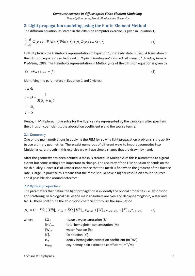
The diffusion equation, as stated in the diffusion computer exercise, is given in Equation 1;

),(),(),(),(),('

1t r S t r t r t r Dt r

dt

d

ca =Φ+Φ∇∇−Φ µ (1)

In Multiphysics the Helmholtz representation of Equation 1, in steady state is used. A translation of

the diffusion equation can be found in “Optical tomtography in medical imaging”, Arridge, Inverse

Problems, 1999. The Helmholtz representation in Multiphysics of the diffusion equation is given by

f auuc =+∇−∇ )( . (2)

Identifying the parameters in Equation 1 and 2 yields:

S f

a

Dc

u

a

sa

=

=

+==

Φ=

µ

µ µ )(3

1'

Hence, in Mutiphysics, one solve for the fluence rate represented by the variable u after specifying

the diffusion coefficient c, the absorption coefficient a and the source term f .

2.1 Geometry

One of the main motivations in applying the FEM for solving light propagation problems is the ability

to use arbitrary geometries. There exist numerous of different ways to import geometries intoMultiphysics, although in this exercise we will use simple shapes that are drawn by hand.

After the geometry has been defined, a mesh is created. In Multiphysics this is automated to a great

extent but some settings are important to change. The accuracy of the FEM solution depends on the

mesh quality. Hence it is of utmost importance that the mesh is fine when the gradient of the fluence

rate is large. In practice this means that the mesh should have a higher resolution around sources

and if possible also around detectors.

2.2 Optical properties

The parameters that define the light propagation is evidently the optical properties, i.e. absorption

and scattering. In biological tissues the main absorbers are oxy- and deoxy-hemoglobin, water and

fat. All these contribute the absorption coefficient through the summation

%100,%%100,%222][][][])[1( F aW a HbOtot Hbtot a F W HbSO HbSO µ µ ε ε µ +++−= (3)

where SO2: tissue oxygen saturation (%)

[Hb]tot total hemoglobin concentration (M)

[W]% water fraction (%)

[F]% fat fraction (%)

εHb deoxy-hemoglobin extinction coefficient (m-1

/M)

εHbO2 oxy-hemoglobin extinction coefficient (m-1

/M)






μa,W100% absorption coefficient at 100% water fraction

μa,F100% absorption coefficient at 100% fat fraction

The reduced scattering can be defined by

SP

s SA−

⋅= )1000 / (' λ µ (4)

where SA: scattering amplitude (related to scatterer density)

SP: scattering power (related to scatterer size distribution)

λ: wavelength in nm

Among the files for the exercise a Matlab-script called ”opticalproperties.m” can be found. Run this

script in Matlab to see how the absorption and reduced scattering properties change when changing

the different parameters above.

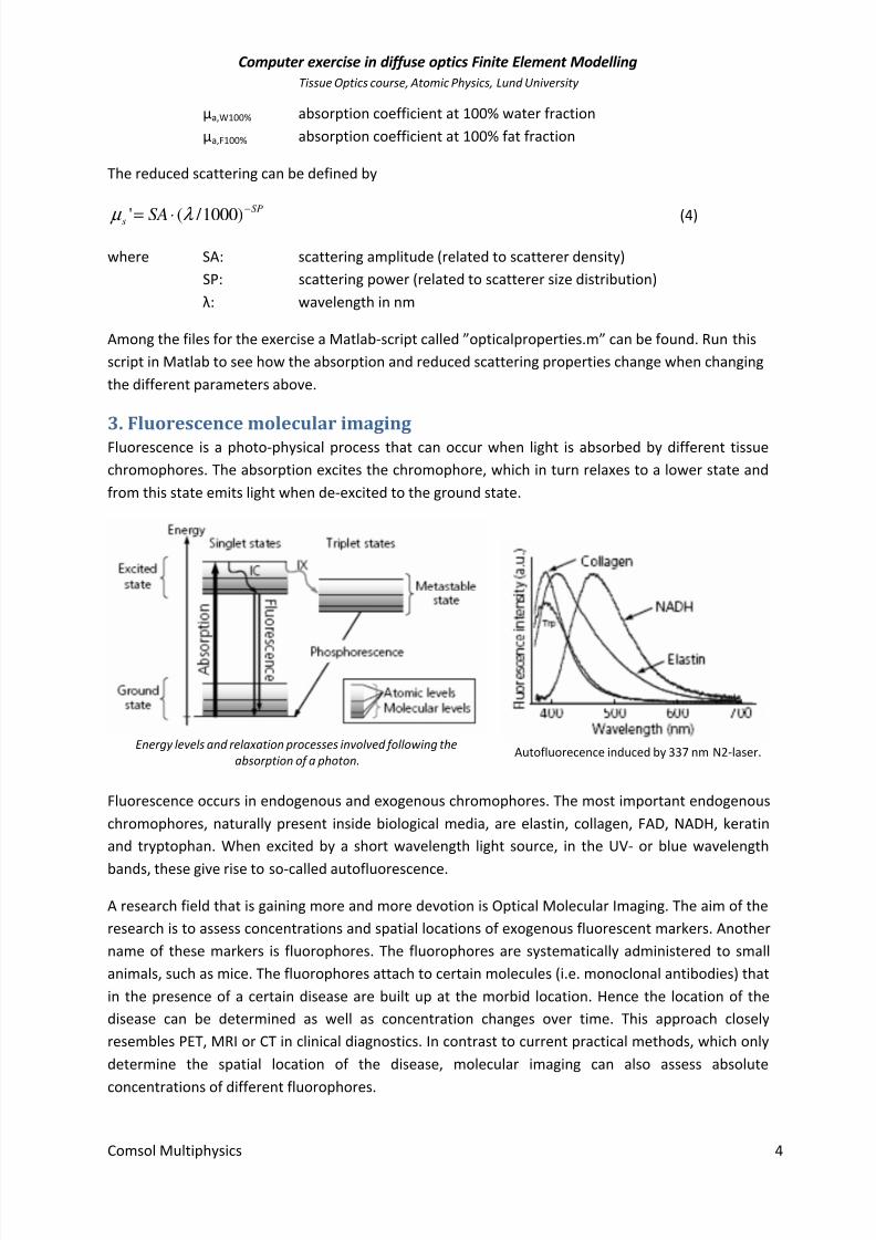
3. Fluorescence molecular imaging

Fluorescence is a photo-physical process that can occur when light is absorbed by different tissue

chromophores. The absorption excites the chromophore, which in turn relaxes to a lower state and

from this state emits light when de-excited to the ground state.

Energy levels and relaxation processes involved following the

absorption of a photon. Autofluorecence induced by 337 nm N2-laser.

Fluorescence occurs in endogenous and exogenous chromophores. The most important endogenous

chromophores, naturally present inside biological media, are elastin, collagen, FAD, NADH, keratin

and tryptophan. When excited by a short wavelength light source, in the UV- or blue wavelength

bands, these give rise to so-called autofluorescence.

A research field that is gaining more and more devotion is Optical Molecular Imaging. The aim of the

research is to assess concentrations and spatial locations of exogenous fluorescent markers. Another

name of these markers is fluorophores. The fluorophores are systematically administered to small

animals, such as mice. The fluorophores attach to certain molecules (i.e. monoclonal antibodies) that

in the presence of a certain disease are built up at the morbid location. Hence the location of the

disease can be determined as well as concentration changes over time. This approach closely

resembles PET, MRI or CT in clinical diagnostics. In contrast to current practical methods, which only

determine the spatial location of the disease, molecular imaging can also assess absolute

concentrations of different fluorophores.






3.1 Fluorophores

There are of course a wide range of fluorophores, each suited for a different application. Commonly

used fluorophores in optical molecular imaging can be viewed here:

http://www.invitrogen.com/site/us/en/home/support/Research-Tools/Fluorescence-SpectraViewer.html.

Extinction and emission properties for some selected fluorophores are seen in the figure below.

Extinction and emission properties of some selected fluorophores

3.2 Modeling fluorescence

To model fluorescence in Multiphysics, one first solves the diffusion equation (a Helmholtz equation)

for the excitation light, which will act as the source term for the fluorescence. The fluorescence light

propagation is then modeled by adding another Helmholtz equation and solving for the fluence rate.

The “emission” Helmholtz equation is given another set of optical properties since the wavelength isdifferent as compared to the excitation light. The following equations in steady-state represent this

in a formal way:

)()()()()( r S r r r Dr x xax x x x =Φ+Φ∇∇−Φ µ (5)

)()()()()( r r r r Dr xmaf mammmm Φ=Φ+Φ∇∇−Φ γ µ µ (6)

Eq. (4) describes the excitation light fluence rate (denoted with subscript x ) while Eq. (4) models the

emission light at one wavelength (denoted with subscript m). Looking carefully on the secondequation’s source term may cause nuisance. µaf is the absorption coefficient at the excitation

wavelength, φx is the excitation fluence rate solved for in Equation 5 and ϒ m is the fluorescence yield

fraction. To understand the yield fraction a closer look at the fluorescence emission spectra in the

figure above. A well-known fact is that all fluorescence is not emitted equally for all wavelengths, i.e.

there is a fluorescence spectrum that describes the probability of emission at a certain wavelength.

E.g. for fluorophore IRDye800 (seen above) the most probable wavelength is 800 nm.






When simulating singe wavelength emission the yield parameter can be set to unity. However, when

performing multispectral fluorescence emission modeling it is important to scale every spectral band

with its correct fluorescence yield fraction.

4. Laser thermotherapy

The effectiveness of various therapeutic methods such as radiotherapy and chemotherapy has been

shown to increase by inducing a temperature elevation of a few degrees above body temperature. At

even higher temperatures cells are rapidly killed. Heat treatment has also been utilized as a surgical

method to coagulate or vaporize tumors in many parts of the body. With the invention of the laser in

1960, a new device to induce heat for medical purposes appeared. Using thin optical fibers the

surgeon can in a minimally invasive way access the whole gastrointestinal canal and the urogenital

tract. Thermal contraction of the treated area results in sealing of small blood vessels, which arrests

hemorrhage (i.e., bleeding).

Hyperthermia is defined as temperatures in the interval of about 41-47oC. In cancer therapy it is

generally recognized that hyperthermia should be combined with another therapeutic method, such

as ionizing radiation, drugs or photodynamic therapy, in order to fully exploit the benefits of the

treatment. At least three distinct effects of hyperthermia contribute to the result, namely the direct

cell kill, the indirect cell kill due to the destruction of microvasculature, and the heat sensitization to

another treatment modality. Tumors show an apparent, albeit slight, increase in sensitivity to heat in

the range 42-44oC as compared with normal tissue. Above 44

oC, the difference in heat sensitivity is

lost. Clinical hyperthermia has therefore been applied in the above temperature range for about one

hour to try to cause tumor cell death while preserving normal tissue.

Thermotherapy employs temperatures, which enable coagulation of the treated tissue. Coagulation

means a denaturation of proteins causing cell death. The process results in an increase in the

scattering properties of tissue (compare with the boiled egg white). Rapid tissue destruction is

accomplished by elevating the tissue temperature above 55oC. No difference in heat sensitivity exists

at this temperature; tumour and normal tissue are destroyed at the same high rate. Therefore, heat

must be applied at precisely the right location not to induce gross normal tissue damage.

Lasers as well as other light sources are used to produce thermal effects in tissue. For heating and

ablation purposes, infrared radiation is used since it is absorbed by water. The infrared region

extends roughly from 300 GHz - 400 THz, which corresponds to wavelengths between 1 mm and 750

nm. Examples of light sources in clinical use are the CO2 (10 µm) and the Nd:YAG lasers (1064 nm).

Visible light is commonly used in ophthalmology and dermatology, the wavelength of visible light

ranging from about 400 nm to 750 nm.

Another parameter, which determines the treatment result, is the pulse length. For heating of large

volumes, as in hyperthermia and thermo-therapy, continuous wave mode is preferentially employed

as thermal dissipation due to conduction is the principal determinant of tissue damage.

4.1 Modeling heat transfer in tissue

In the context of tissue heat treatment the four principal modes of heat transfer are conduction,

convection, radiation and evaporation. This section briefly describes the different modes. Conduction

is an intrinsic property of the medium, whereas evaporation acts as a boundary condition at tissue-






air boundaries. Radiation and convection are present to varying degrees both inside the bulk tissue

and at surfaces.

Thermal conduction is transfer of energy from the more energetic particles in a substrate to the

adjacent less energetic ones as a result of interactions between the particles. This mode of tissue

heat transfer is described by Fourier’s law, which states that the heat flow at a given point in thetissue is proportional to the gradient of the temperature. An energy balance for a volume element

gives the following relation for transient conduction

( )T t

T C ∇∇=∂

∂λ ρ (7)

where ρ (kg m-3

) is the density, C (J kg-1

K-1

) is the specific heat capacity, λ (W m-1

K-1

) is the thermal

conductivity, and T (K) is the tissue temperature. The ratio λ/(ρc) is called the thermal diffusivity, α

(m2

s-1

), which describes the dynamic behavior of the thermal process.

The thermal properties depend on the type of tissue and temperature. Since most tissues can be

considered as being composed of a combination of water, proteins and fat, the magnitude of the

conductivity can be estimated with knowledge of the proportions of these components. The table

below shows selected data on the thermo-physical properties of tissue measured at room or body

temperature. It can be observed that of the different components constituting tissue, water has the

highest values of the thermal conductivity and diffusivity. Therefore, tissues with high water content

are the best thermal conductors and respond the fastest to a thermal disturbance.

Material Conductivity

(W m-1

K-1

)

Density

(kg m-3

)×10-3

Specific heat

(kJ kg-1

K-1

)

Diffusivity

(m2

s-1

) ×107

Muscle 0.38-0.54 1.01-1.05 3.6-3.8 0.90-1.5

Fat 0.19-0.20 0.85-0.94 2.2-2.4 0.96

Kidney 0.54 1.05 3.9 1.3

Heart 0.59 1.06 3.7 1.4

Liver 0.57 1.05 3.6 1.5

Brain 0.16-0.57 1.04-1.05 3.6-3.7 0.44-1.4

Water @ 37oC 0.63 0.99 4.2 1.5

Thermo-physical properties of human tissue and water

Convection is the term applied to heat transfer between a surface and a fluid, e.g., air or blood,

moving over the surface. Convection problems involve heat transfer between the surface of the bodyand the surrounding air and also between blood and the vessel wall. The heat transfer between a

conducting solid, which in this context is tissue and a convective fluid is usually described using

Newton’s law of cooling which states that the heat flow q (W m-2

) normal to the surface is

proportional to the temperature difference between the surface T (K) of the tissue and the bulk

temperature of the fluid T ∞:

( )∞−= T T hq (8)

where the proportionality constant, h (W m-2

K-1

), is called the local heat convection coefficient. As

shown in the figure below there exist a thermal boundary layer if the fluid free stream temperatureand the temperature of the tissue differ.






Schematic picture of the thermal boundary layer.

At the tissue surface there is no fluid motion and energy transfer occurs only by conduction. The

magnitude of the heat convection coefficient therefore depends on the temperature gradient at the

surface but also on the conditions in the boundary layer. Equations can be set up to account for the

physical processes in the boundary layer but the solutions readily become very complex. Here it

suffices just to give examples of the convection coefficient in a few cases;

Mode h (W/m2/K)

Free convection

(tissue – air)

5-25

Forced convection

(tissue – air, i.e. a windy day)

50-20 000

convection with phase change (boiling) 2500 – 100 000

Values of the convection coefficient for a few cases

Radiation is emitted from every body and the electromagnetic radiation is proportional to the fourth

power of the absolute temperature. The maximum heat flow, q (W m

-2

) emitted from a black body isexpressed by:

( )44

∞−= T T q sεσ (9)

where σ (W m-2

K-4

) is the Stefan-Boltzmann constant, T s and T ∞ (K) are the tissue surface and

environmental temperature, respectively and ε is the emissivity. Since tissue is not a perfect black

body the emissivity is less than one. For human skin, the value of the emissivity is in the range 0.98-

0.99. When modeling internal biological tissue, intrinsic radiative heat transfer processes constitute a

negligible contribution and the process of radiation is often considered only a boundary effect.

Evaporation is the process where moist tissue, in contact with air, is subject to heat loss associated

with evaporation of water. The driving force for the loss of tissue moisture by diffusion is the

difference in water concentration between the tissue and the surrounding air. For ideal gas mixtures,

such as air and water vapour, the concentration of a component is proportional to the partial

pressure. The water at the tissue surface is in thermodynamic equilibrium with the water vapour in

air, i.e., at the surface the pressure of the water vapour is equal to the saturated water vapour

pressure at the surface temperature. Therefore, water will migrate from the tissue surface to the air

if the saturated vapour pressure at the surface is greater than the partial pressure of vapour in the

surrounding air. Evaporation acts as a loss term in the bio-heat equation at tissue surfaces.






The Bio-heat equation is the governing equation that describes the heat transfer in tissue and is

defined by

( )m ps QQQT

t

T C +++∇∇=∂

∂λ ρ (10)

Here Q s is the heat source within the medium, e.g. absorbed light due to laser irradiation, Q p is the

heat gained or lost due to blood perfusion and Q m is the heat source due to metabolic activity.

Convection between tissue surface and surrounding air, radiation and evaporation are processes that

have to be modeled as appropriate boundary conditions.

In Comsol Multiphysics, the bio-heat equation is modeled by a physics mode (appropriately) called

“Bioheat Transfer ” and defined by the equation

( ) ( )met bbbbtrans p p QT T C T k T uC

t

T C +−+∇∇=∇⋅+

∂

∂ω ρ ρ ρ (11)

Some parameters need explanation in Eq. (11). transu is a translational motion vector that can be

used for modeling moving heat transfer phenomena. We will not consider this here. A comparison

between Eq. (9) and (10) concludes that( )T T C Q bbbb p −= ω ρ

, i.e. the heat lost or gained by blood

perfusion in the tissue. Here Tb (K) is the temperature of the arterial blood and ωb is the blood

volumetric perfusion rate in (s-1

). Typical values for the blood perfusion is 10-60 ml/min per 100g of

tissue. This corresponds to a volumetric perfusion rate of 0.002 – 0.01 s-1

.






5. Tutorial 1: Modeling light fluence rate from a point source in a slab

In this tutorial a light source incident on the boundary of a slab is simulated. One can think of this as

an optical fiber positioned at the surface of an object. In Comsol Multiphsyics we can model this by

creating a slab and assign a point source as a light source. Start Multiphysics.

5.1 The model wizard

At program startup a wizard guides you through the selections that are required to setup a model.

5.1.1 Space dimension

Select space dimension 3D. Click blue arrow in the top right corner (see figure below) to proceed.

Space dimension, click the blue arrow to proceed to next panel

5.1.2 Add physics

In the menu, select Mathematics > Classical PDEs > Helmholtz Equation (hzeq)

5.1.3 Study type

Select Stationary analysis. Click the ”goal flag” when done

5.2 Model builder

You should now have a left menu looking like this:

Model builder menu






5.2.1 Global definitions

This is where parameters, variables and functions are set. These can be used throughout the

modeling. For example it is convenient to define the optical properties in the Parameters panel.

5.2.1.1 Parameters

Right click Global definitions and select Parameters from the menu. Define the Parameters in thepanel. An example can be seen in the figure below.

Global definitions > Parameters (Remember that all units are in SI units, i.e. the optical properties are 1/m)

5.2.2 Model1 (mod1)

The next menu item is called Model1 (mod1) by default. This is where the geometry, boundary

conditions and mesh parameters are defined.

5.2.2.1 Definitions

Here local variables can be defined that are private to the current model. We can skip this for now.

5.2.2.2 Geometry

The geometry needs to be created. Comsol Multphysics can import CAD-drawings but here we will

rely on user-made simple geometry shapes.

Make a slab: Right click the Geometry1 menu item and select Block. Next, set the properties of the

block, e.g.

- Object type: solid (surface can be selected but in that case the slab will be hollow)

- Size and Shape: [Width, Depth, Height] = [0.05, 0.05 0.02] (remember the units are in SI, i.e.

all lengths are in meters)

- Position: Select Center at [x,y,z]=[0, 0, 0.01]. This makes the Origo at the incident boundary

which is the most convenient.

Leave the other options as default. In order to draw the geometry; click the icon ”Build selected” in

the upper right corner, i.e.

Make a point: The light source is defined by a point source positioned one scattering length inside

the boundary. In order to create this point; Right click the Geometry1 menu item and select More

Primitives > Point. Here you can select where the point will be located, i.e. [x,y,z]=[0,0,1/musp].

Click ”Build selected” in order to place the point on the workspace.






Since the point is inside the slab we can’t see it. In order to make the

geometry shapes transparent, click the ”Transparency” icon in the

upper right corner of the Comsol window, see figure to the right.

5.2.2.3 Materials

If you have large libraries with materials you can assign different materials to parts of the geometry.

However we define the optical properties manually and do not use this menu.

5.2.2.4 Helmholtz Equation (hzeq)

The diffusion equation needs boundary conditions and at least one source term in order to be solved.

Assign optical properties: Expand the PDE (hzeq) menu and click the ”Helmholtz Equation 1” menu

item. The panel that appears is seen in the figure below.

Here you can select the domain in which the equation is to be solved, by default this is set to all

domains and we should keep it like that. The Helmholtz equation can be seen in the ”Equation-tab”

where terms (c, f and a) are defined.






- Define the diffusion coefficient by setting c = D. We have defined D in Global Definitions >

Parameters, if not you should input a value here.

- Define the source term by setting f=0. The source term should be zero here since this term

holds for the whole geometry. We will use a point source instead that we will define later in

this tutorial.

- Define the absorption term by setting a=mua. We have defined mua in Global Definitions >

Parameters, if not you should input a value here.

Assign boundary conditions: The ”Zero Flux 1” menu item defines a boundary condition. However,

this condition states that the fluence rate is zero at the boundary. This is evidently not correct since

we should simulate reflection, induced by refractive index mismatch, at the boundary. A Robin-type

boundary condition should be used instead. Right click PDE (hzeq) and select Flux/Source boundary

condition. First we need to select the boundaries where this condition holds.

- In the Boundary Selection tab select ”All boundaries” (in the drop down menu)

Expand the Equation tab in order to look at the boundary condition. Identification with the Robin-

type diffusion equation boundary condition reveals that;

- Boundary Flux/Source term should be set to g=0.

- Boundary Absorption/Impedance term should be set to q=1/(2*A). (We have defined

A=2.74 in the Global Definitions > Parameters).

Now, it looks like we have two boundary conditions in the left menu, i.e. ”Zero Flux” and

”Flux/Source”. However this is not the case. Click ”Zero Flux” and you will see ”(overridden)” after

each boundary. This means that another boundary condition will be assigned to the problem (in our

case it is the Flux/Source).

Assign a point source: A light source is needed and we have mentioned before that the point placed

in the center should be for this purpose. Right click the PDE (hzeq) menu item and then Points >

Point Source.

- Point selection: In the drawing window mark the point using the mouse so that it changes

color. In the Point selection tab click the ”plus sign”. A number will then appear in the point

selection tab, e.g. 5 but the numbering depends on how the coordinate system is defined.

- Source term: Assign a value in [W], e.g. f=0.1 for 100 mW.

The physics parameters are all set, now we need to create the mesh.

5.2.2.5 Mesh 1

The mesh can obviously be defined in a multitude of ways and in this exercise we will only touch

upon the surface of the world of meshing. However it is important to realize that the mesh

determines the accuracy of the solution. If a too coarse mesh is used the diffusion equation solution

is most likely erroneous due to discretization errors. On the other hand going for the finest resolution

of the mesh directly will render a large number of mesh elements that many computers can’t store in

memory.






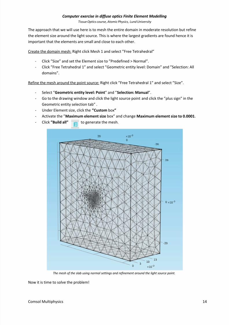
The approach that we will use here is to mesh the entire domain in moderate resolution but refine

the element size around the light source. This is where the largest gradients are found hence it is

important that the elements are small and close to each other.

Create the domain mesh: Right click Mesh 1 and select ”Free Tetrahedral”

- Click ”Size” and set the Element size to ”Predefined > Normal”.

- Click ”Free Tetrahedral 1” and select ”Geometric entity level: Domain” and ”Selection: All

domains”.

Refine the mesh around the point source: Right click ”Free Tetrahedral 1” and select ”Size”.

- Select ”Geometric entity level: Point” and ”Selection: Manual”.

- Go to the drawing window and click the light source point and click the ”plus sign” in the

Geometric entity selection tab” .

- Under Element size, click the ”Custom box”

- Activate the ”Maximum element size box” and change Maximum element size to 0.0001.

- Click ”Build all” to generate the mesh.

The mesh of the slab using normal settings and refinement around the light source point.

Now it is time to solve the problem!






5.2.3 Study 1

Right click the ”Study 1” menu item in the left menu and select ”Compute”. Wait for completion.

5.2.4 Results

The solution is contained in the variable ”u” as defined by the Helmholtz equation.

View the solution: A menu item under “Results > 3D Plot Group 2 > Slice 1” should have been

created after the solver completes. Otherwise, right click the ”Results” menu and select ”3D Plot

group”. Right click the ”3D Plot group” and select ”Slice”. In the panel,

- Select Data set: Solution 1 (or From parent)

- Change the Expression: to ”log(u)” in order to view the logarithm of the solution.

- Select in what plane the solution should be plotted and the number of planes. Keeping the

default is not a bad idea to start with.

- Click the Plot icon in the upper right corner of the panel.

View a line plot of the solution: Sometimes (quite often) it is valuable to look at the solution along aline on the boundary or through the geometry. In order to plot a line

- Right click Results > Data sets and select Cut line 3D

- In the panel; set ”Data set: Solution 1”

- Set the coordinates to x= [-0.025 0.025], y = [0 0] and z = [0.02 0.02].

- Right click Results > Data sets and select 1D Plot Group

- Right click the 1D Plot Group and create a Line Graph

- Select the “Cut Line 3D” dataset as you created above in the drop down menu.

- Set the expression to ”u” or ”log(u)”. Test both.

- Click the Plot icon in the upper right corner of the panel .

- Also create a line plot in the same way at x= [-0.025 0.025], y = [0 0] and z = [0 0].- You should get a plot looking like the figure below.






Questions

• In the figure above you see the solutions at the incidence boundary (i.e. the Remittance*)

and the far boundary (i.e. the Transmittance) relative the light source. It seems that there are

some wiggles in the solution, most prominently in the Remittance plot. Why?

• What would you do to get rid of these? Do it!

When using higher mesh resolution there is a risk that the memory of the computer is not

enough. By default Comsol Multiphysics uses Direct solvers but changing to Iterative solver

method can enable solutions of larger problems. The price to pay is that it takes longer time

to solve the problem. To change the solver to Iterative solver;

Right click “Stationary Solver 1” > Select “Iterative” solver. Keep all settings as default.

• Until now we have simulated light at one wavelength incident on the boundary of the slab.

How would you suggest implementing a white light source incident on the boundary? Discuss

with your partner and instructor.

*Remittance is the same as Diffuse Reflectance






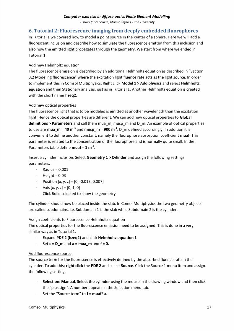
6. Tutorial 2: Fluorescence imaging from deeply embedded fluorophores

In Tutorial 1 we covered how to model a point source in the center of a sphere. Here we will add a

fluorescent inclusion and describe how to simulate the fluorescence emitted from this inclusion and

also how the emitted light propagates through the geometry. We start from where we ended in

Tutorial 1.

Add new Helmholtz equation

The fluorescence emission is described by an additional Helmholtz equation as described in “Section

3.2 Modeling fluorescence” where the excitation light fluence rate acts as the light source. In order

to implement this in Comsol Multiphysics, Right click Model 1 > Add physics and select Helmholtz

equation and then Stationary analysis, just as in Tutorial 1. Another Helmholtz equation is created

with the short name hzeq2.

Add new optical properties

The fluorescence light that is to be modeled is emitted at another wavelength than the excitation

light. Hence the optical properties are different. We can add new optical properties to Global

definitions > Parameters and call them mua_m, musp_m and D_m. An example of optical properties

to use are mua_m = 40 m-1 and musp_m = 900 m-1, D_m defined accordingly. In addition it is

convenient to define another constant, namely the fluorophore absorption coefficient muaf . This

parameter is related to the concentration of the fluorophore and is normally quite small. In the

Parameters table define muaf = 1 m-1.

Insert a cylinder inclusion: Select Geometry 1 > Cylinder and assign the following settings

parameters:

- Radius = 0.001

- Height = 0.03

- Position [x, y, z] = [0, -0.015, 0.007]

- Axis [x, y, z] = [0, 1, 0]

- Click Build selected to show the geometry

The cylinder should now be placed inside the slab. In Comol Multiphysics the two geometry objects

are called subdomains, i.e. Subdomain 1 is the slab while Subdomain 2 is the cylinder.

Assign coefficients to Fluorescence Helmholtz equation

The optical properties for the fluorescence emission need to be assigned. This is done in a very

similar way as in Tutorial 1.- Expand PDE 2 (hzeq2) and click Helmholtz equation 1

- Set c = D_m and a = mua_m and f = 0.

Add fluorescence source

The source term for the fluorescence is effectively defined by the absorbed fluence rate in the

cylinder. To add this; right click the PDE 2 and select Source. Click the Source 1 menu item and assign

the following settings

- Selection: Manual, Select the cylinder using the mouse in the drawing window and then click

the “plus sign”. A number appears in the Selection menu tab.

- Set the “Source term” to f = muaf*u.






This source term makes the cylinder act as a light source with the strength “muaf*u” where u is the

excitation light fluence rate in the cylinder.

Add boundary conditions

The boundary conditions needs to be set. Do this in the same way as Tutorial 1, however make sure

that it is only the outer boundaries that are assigned the Flux/Source condition. Comsol Multisphysicsmakes it possible to choose internal boundaries, however this is not what we want.

Since a second subdomain has been added to the geometry the boundary conditions for Helmholtz

equation 1 (hzeq) also needs to be updated so that only the external boundaries are included in the

condition.

Make a mesh

As we did in Tutorial 1.

Solve the problem

Right click Study 2 and click Compute. If the solver runs into problems, e.g. not enough memory,

change the solver to Iterative solver instead (see question part last in Tutorial 1 for guide how to do

this).

View the solution

Two new plot groups have new been created, i.e. 3D Plot Group 4 and 3D Plot Group 5, both of them

containing excitation light (u) and emission light (u2). Plot the solutions (u and u2) by changing the

Expression. Try for example to make slice plots of u, log(u), u2 and log(u2).

Questions

• Study the solution and explain why the fluorescence emission does not look like a cylinder,discuss with your partner and instructor.

• Change the depth of the cylinder (i.e. move the cylinder to other z-coordinates, don’t forget

to make a new mesh after you have changed the geometry). Explain what happens with the

spatial distribution of the emission intensity as the cylinder is closer to the far boundary

(relative the point source).

• How would you simulate a fluorophore with a specific emission spectrum? i.e. how do you

define the spectrum in Comsol Multiphysics?

• How would you simulate autofluorescence?






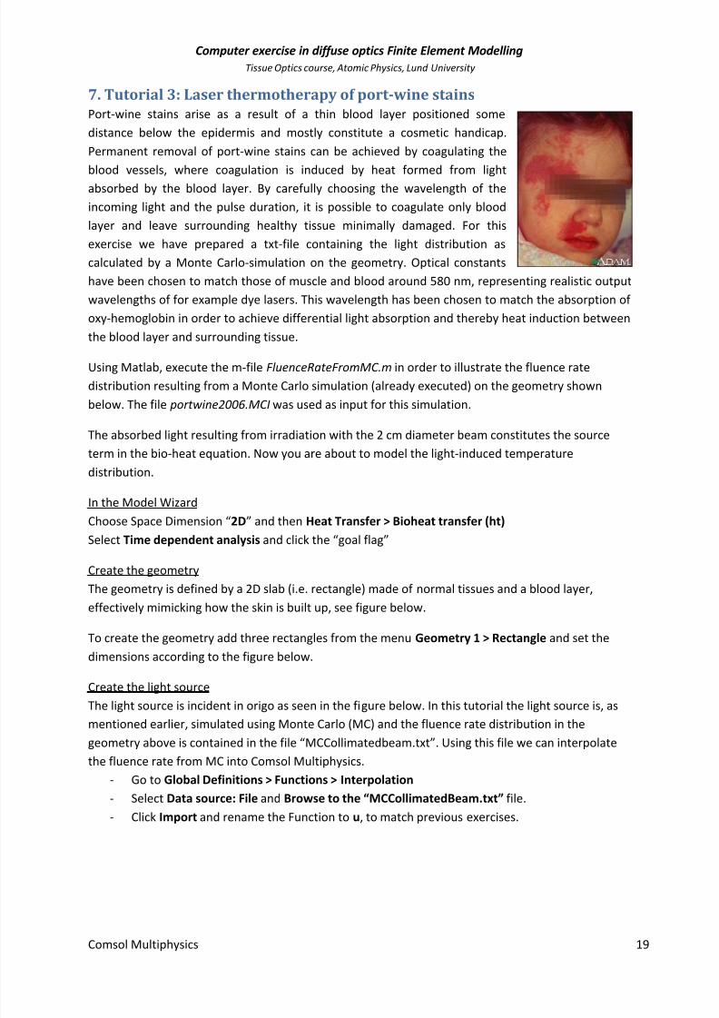
7. Tutorial 3: Laser thermotherapy of port-wine stains

Port-wine stains arise as a result of a thin blood layer positioned some

distance below the epidermis and mostly constitute a cosmetic handicap.

Permanent removal of port-wine stains can be achieved by coagulating the

blood vessels, where coagulation is induced by heat formed from light

absorbed by the blood layer. By carefully choosing the wavelength of the

incoming light and the pulse duration, it is possible to coagulate only blood

layer and leave surrounding healthy tissue minimally damaged. For this

exercise we have prepared a txt-file containing the light distribution as

calculated by a Monte Carlo-simulation on the geometry. Optical constants

have been chosen to match those of muscle and blood around 580 nm, representing realistic output

wavelengths of for example dye lasers. This wavelength has been chosen to match the absorption of

oxy-hemoglobin in order to achieve differential light absorption and thereby heat induction between

the blood layer and surrounding tissue.

Using Matlab, execute the m-file FluenceRateFromMC.m in order to illustrate the fluence rate

distribution resulting from a Monte Carlo simulation (already executed) on the geometry shown

below. The file portwine2006.MCI was used as input for this simulation.

The absorbed light resulting from irradiation with the 2 cm diameter beam constitutes the source

term in the bio-heat equation. Now you are about to model the light-induced temperature

distribution.

In the Model Wizard

Choose Space Dimension “2D” and then Heat Transfer > Bioheat transfer (ht)

Select Time dependent analysis and click the “goal flag”

Create the geometry

The geometry is defined by a 2D slab (i.e. rectangle) made of normal tissues and a blood layer,

effectively mimicking how the skin is built up, see figure below.

To create the geometry add three rectangles from the menu Geometry 1 > Rectangle and set the

dimensions according to the figure below.

Create the light source

The light source is incident in origo as seen in the figure below. In this tutorial the light source is, as

mentioned earlier, simulated using Monte Carlo (MC) and the fluence rate distribution in the

geometry above is contained in the file “MCCollimatedbeam.txt”. Using this file we can interpolate

the fluence rate from MC into Comsol Multiphysics.

- Go to Global Definitions > Functions > Interpolation

- Select Data source: File and Browse to the “MCCollimatedBeam.txt” file.

- Click Import and rename the Function to u, to match previous exercises.






The simulation geometry in Tutorial 3 mimicking skin.

Insert parameters

In Global Definitions > Parameters assign the parameters that you need, i.e. the ones that are

defined in the figure above.

Create the geometry

Create a 2D slab according to the figure above. Carefully look so that you get the coordinate systemright. Also note that the slab actually consists of three rectangles of different thicknesses. From the

laser incidence boundary, these are surface layer, blood layer and bulk tissue layer. It is important to

create the geometry in exactly this way since it should correspond to the MC-simulation of the laser

light fluence rate.

Assign physical heat transfer parameters

Under Heat transfer all the physical parameters should be set.

“Biological tissues”; bulk tissue

- Click the Biological tissue 1 and fill in the parameters “thermal conductivity”, “density” and

“heat capacity” for the surface and tissue layers. These two layers are defined by Domain 1

and 3. The proper values can be found in the figure describing the simulation geometry.

- Click Biological tissue 1 > Bioheat 1 and assign the perfusion properties of blood. This is

optional and we can assume that the blood is static.

“Biological tissues”; blood

- Add another tissue through Heat transfer > Biological tissue and assign parameters for the

blood layer in the same way as above. The blood layer is defined by Domain 2.

Two heat sources

- Right click Heat transfer > Heat source, do this so that you create two heat sources.






- For one of the heat sources select domains 1 and 3 (tissue layer) and for the other select 2

(blood layer).

- The heat sources should equal the imported variable, u(x,y) (write exactly like this!),

multiplied by the absorption coefficient in the specific tissue and the laser power (100 W not

unrealistic in a clinical setting!).

Convective cooling at the outer tissue-air boundary

- Click Heat transfer > Convective cooling

- Select the boundaries where the boundary condition should hold. At the tissue-air boundary

assume free convection with h = 20 W/m2K and assume room temperature as external

temperature

Fixed temperature at the internal tissue-tissue boundaries

- Click Heat transfer > Temperature

- Select the boundaries where the boundary condition should hold. For simplicity we assume a

constant body temperature and the tissue – tissue boundaries. This is reasonable since thenwe assume that the small portion of the tissue that we simulate is in thermal equilibrium

with the rest of the body.

Finally we note that we ignore other boundary conditions such as radiation and inward heat flux.

Initial temperature

Set Heat transfer > Initial Values to body temperature

Introduce a mesh

Create a mesh using “finer” setting (or “extra fine” if possible).

Solve the problem

Observe that the physics mode chosen is a time dependent problem (why?) and that we need to

specify how long the laser pulses are. This is done via Study 1 > Step 1: Time Dependent and Times,

which should be written range(0,0.01,0.1) which means that Comsol Multiphysics solves the problem

at times between 0 and 0.1 seconds with increments of 0.01s. Start the solver.

View the solution

Plot the solution along a line (create a “2D Cut line” under Results > Data sets). Plot the results from

[x,y] = [0,0] to [x,y] = [0,0.002].

Questions• By looking at the line plot, can you determine whether the blood vessels are coagulated?

• The requirements are to coagulate the blood layer while sparing surrounding tissue. Repeat

the same simulation with a 1 second pulse. Can you say what is to prefer from a therapeutic

point of view; prolonging the laser pulse or increasing the pulse power?

• What can be done in order to save the skin surface? In a clinical setting the doctor cools the

skin before treating. Perform the same simulation assuming a constant temperature of 10oC

at the skin surface. How does this influence the treatment volume?

Multi Physics Exercise

Documents

Transcript of Multi Physics Exercise