Multi-objective operation management of a renewable MG ... · Multi-objective operation management...

Aalborg Universitet

Multi-objective Operation Management of a Renewable Micro Grid with Back-up MicroTurbine/Fuel Cell/Battery Hybrid Power Source

Anvari-Moghaddam, Amjad; Seifi, Alireza; Niknam, Taher; Alizadeh Pahlavani,MohammadrezaPublished in:Energy

Publication date:2011

Link to publication from Aalborg University

Citation for published version (APA):Anvari-Moghaddam, A., Seifi, A., Niknam, T., & Alizadeh Pahlavani, M. (2011). Multi-objective OperationManagement of a Renewable Micro Grid with Back-up Micro Turbine/Fuel Cell/Battery Hybrid Power Source.Energy, 36(11), 6490-6507.

General rightsCopyright and moral rights for the publications made accessible in the public portal are retained by the authors and/or other copyright ownersand it is a condition of accessing publications that users recognise and abide by the legal requirements associated with these rights.

? Users may download and print one copy of any publication from the public portal for the purpose of private study or research. ? You may not further distribute the material or use it for any profit-making activity or commercial gain ? You may freely distribute the URL identifying the publication in the public portal ?

Take down policyIf you believe that this document breaches copyright please contact us at [email protected] providing details, and we will remove access tothe work immediately and investigate your claim.

https://vbn.aau.dk/en/publications/aedb3fc4-6be3-4b9c-8d0b-4bb7af51830b

at SciVerse ScienceDirect

Energy 36 (2011) 6490e6507

Contents lists available

Energy

journal homepage: www.elsevier .com/locate/energy

Multi-objective operation management of a renewable MG (micro-grid) withback-up micro-turbine/fuel cell/battery hybrid power source

Amjad Anvari Moghaddama, Alireza Seifi a, Taher Niknamb,*, Mohammad Reza Alizadeh Pahlavani c

aDepartment of Power & Control, School of Electrical and Computer engineering, Shiraz University, Engineering Faculty No.1, Zand St., Shiraz, IranbDepartment of electrical and electronics engineering, Shiraz University of Technology, Shiraz, IrancDepartment of Electrical Engineering, Iran University of Science and Technology (IUST), Tehran, Iran

a r t i c l e i n f o

Article history:Received 14 March 2011Received in revised form6 September 2011Accepted 10 September 2011Available online 14 October 2011

Keywords:PSO (Particle swarm optimization)Chaotic searchMulti-operation managementMicro-gridRESs (Renewable energy sources)

* Corresponding author. Tel.: þ98 711 2337852; faxE-mail addresses: [email protected] (A.A. Mog

(A. Seifi), [email protected], [email protected]

0360-5442/$ e see front matter � 2011 Elsevier Ltd.doi:10.1016/j.energy.2011.09.017

a b s t r a c t

As a result of today’s rapid socioeconomic growth and environmental concerns, higher service reliability,better power quality, increased energy efficiency and energy independency, exploring alternative energyresources, especially the renewable ones, has become the fields of interest for many modern societies. Inthis regard, MG (Micro-Grid) which is comprised of various alternative energy sources can serve asa basic tool to reach the desired objectives while distributing electricity more effectively, economicallyand securely. In this paper an expert multi-objective AMPSO (Adaptive Modified Particle Swarm Opti-mization algorithm) is presented for optimal operation of a typical MG with RESs (renewable energysources) accompanied by a back-up Micro-Turbine/Fuel Cell/Battery hybrid power source to level thepower mismatch or to store the surplus of energy when it’s needed. The problem is formulated asa nonlinear constraint multi-objective optimization problem to minimize the total operating cost and thenet emission simultaneously. To improve the optimization process, a hybrid PSO algorithm based ona CLS (Chaotic Local Search) mechanism and a FSA (Fuzzy Self Adaptive) structure is utilized. Theproposed algorithm is tested on a typical MG and its superior performance is compared to those fromother evolutionary algorithms such as GA (Genetic Algorithm) and PSO (Particle Swarm Optimization).

� 2011 Elsevier Ltd. All rights reserved.

1. Introduction

In recent years, the application of alternative energy sourcessuch as wind, biomass, solar, hydro and etc. has become morewidespread mainly due to needs for better reliability, higher powerquality, more flexibility, less cost and smaller environmental foot-prints. On the other hand, DGs (Distributed Generations) such as PV(photovoltaics), micro-turbines, fuel cells and storage devices areexpected to play an important role in future electricity supply andlow carbon economy [1,2]. However, high penetration of DGs intothe grid environment will bring new challenges for the safe andefficient power system operation. These challenges can be partiallyaddressed by MG (Micro-Grid) which is defined as an aggregationof DGs, electrical loads and generation interconnected amongthemselves and with distribution network as well [2e5]. In thisregard, the methodologies applied to manage and control theoperation of MGs are going through continuous changing in order

: þ98 711 6473575.haddam), [email protected](T. Niknam).

All rights reserved.

to make these networks optimized and active systems, thereforethere is a strong need for more precise scheduling of energy sourcesin MGs considering different objectives.

So far, numerous scientific works have been developed byresearchers dealt with the optimal operation scheduling underdifferent loading conditions and objectives. At first, conventionaleconomic scheduling has been proposed as a solution for theoptimization problem through finding an optimal set of generatorsto satisfy load demand and operational constraints in an econom-ical manner [6e8]. Due to the environmental concerns andpollutants emission from traditional fossil fuel units, single-objective optimization could no longer be satisfactory in thementioned problem. To involve emission as a separate goal, multi-objective optimization techniques have been developed in articlesin order to choose a definite number of units for supplying the loadunder a certain condition taking into account minimum levels ofcost and emission for grid operation [9e13]. Recently, evolutionaryalgorithms such as GA (Genetic Algorithm), PSO (Particle SwarmOptimization) and so on have been increasingly proposed forsolving the optimization problem because of their inherentnonlinear mapping, simplicity and powerful search capabilities[13e18]. Hybrid approaches such as Fuzzy-based evolutionary

mailto:[email protected]




www.sciencedirect.com/science/journal/03605442

http://www.elsevier.com/locate/energy

http://dx.doi.org/10.1016/j.energy.2011.09.017



Nomenclature

X vector of the optimization variablesn total number of optimization variablesT total number of hoursNg total number of generation unitsNs total number of storage unitsNk total number of load levelsui(t) status of unit i at hour tPGi(t) active power output of ith generator at time tPsj(t) active power output of jth storage at time tPGrid(t) active power bought/sold from/to the utility at time tBGi(t) bid of the ith DG source at hour tBsj(t) bid of the jth storage options at hour tBGrid(t) bid of utility at hour tSGi start-up/shut-down costs for ith DG unitSsj start-up/shut-down costs for jth storage deviceEGi(t) emissions in kgMWh�1 for ith DG unit at hour tEsj(t) emissions in kgMWh�1 for jth storage device at hour tEGrid(t) emissions in kgMWh�1 for utility at hour tCO2DGi

ðtÞ carbon dioxide pollutants of ith DG unit at hour tSO2DGi

ðtÞ sulfur dioxide pollutants of ith DG unit at hour tNOxDGi

ðtÞ nitrogen oxide pollutants of ith DG unit at hour tCO2Storagej

ðtÞ carbon dioxide pollutants of jth storage device athour t

SO2StoragejðtÞ sulfur dioxide pollutants of jth storage device at hourt

NOxStoragejðtÞ nitrogen oxide pollutants of jth storage device athour t

CO2GridðtÞ carbon dioxide pollutants of utility at hour t

SO2GridðtÞ sulfur dioxide pollutants of utility at hour t

NOxGrid ðtÞ nitrogen oxide pollutants of utility at hour tPLk the amount of kth load levelPG,min(t) minimum active power production of ith DG at hour tPs,min(t) minimum active power production of jth storage at

hour tPgrid,min(t) minimum active power production of the utility at

hour tPG,max(t) maximum active power production of ith DG at hour tPs,max(t) maximum active power production of jth storage at

hour tPgrid,max(t) maximum active power production of the utility at

hour tWess,t battery energy storage at time t

PCharge(Pdischarge) permitted rate of charge (discharge) througha definite period of time

hcharge(hdischarge) charge (discharge) efficiency of the batteryWess,min(Wess,max) lower (upper) bounds on battery energy

storagePcharge,max(Pdischarge,max) maximum rate of charge (discharge)

during each time intervalu inertia weightC1, C2 weighting factors of the stochastic acceleration terms

(Learning factors)rand ($) random function in the range of [0,1]Pbest i best previous experience of the ith particle that is

recordedGbest best particle among the entire populationF vector of objective functionsfi(X) ith objective functiongi(X) equality constraints of ith objective functionhi(X) inequality constraints of ith objective functionVkþ1i updated velocity vector of ith particle

Xkþ1i updated position of ith particle

cxji the jth chaotic variableNchoas number of individuals for CLSX0cls initial population for CLS

NSwarm number of the swarmsDu weight correction valueNBF Normalized Best FitnessBFmin minimum fitness valueBFmax maximum fitness value

List of abbreviationsAMPSO Adaptive Modified Particle Swarm OptimizationFSAPSO Fuzzy Self Adaptive PSOCPSO Chaotic Particle Swarm OptimizationDG Distributed GenerationDER Distributed Energy ResourceRES Renewable Energy SourceMG Micro-gridMGCC (mcc) Micro-grid Central ControllerCLS Chaotic Local SearchWT Wind TurbinePV PhotovoltaicPAFC Phosphoric Acid Fuel CellNiMH-Battery Nickel-Metal-Hydride BatteryMT Micro-Turbine

A.A. Moghaddam et al. / Energy 36 (2011) 6490e6507 6491

algorithms have been also used in scientific literatures many times[19e22]. Similarly, taking a comprehensive look at power dispatchtechniques considering ON/OFF states of generation units showsthat different optimization methods have been proposed to solvethe mentioned problem [23e30]. Among these methods, Senjyuet al. [23] has used a priority list approach for handling the dispatchproblem. Although such method saves the time, it gives scheduleswith relatively higher operation cost. Similarly, BB (Branch-and-Bound)method [24,25] may have some deficiencies handling large-scale problems. LR (Lagrangian Relaxation) method [27e30]focuses on finding an appropriate co-ordination technique forgenerating feasible primal solutions, while minimizing the dualitygap. On the other hand, meta-heuristic methods (e.g., TS (TabuSearch), EP (Evolutionary Programming), SA (simulated annealing),and so on) are iterative techniques that are frequently used inoptimal power dispatch problems [31e35]. Such methods cansearch both local optimal solutions and the global one dependingon the problem domain and time limit.

Due to the population-based search capability as well assimplicity, convergence speed, and robustness, PSO-based optimi-zation algorithms, are widely used for handling multi-objectiveoptimization problems, although the performance of a conven-tional PSO algorithm greatly depends on its parameter and it mayface the danger of being trapped in local optima [36e41]. To handlethese issues suitably and improve the performance of a conven-tional PSO algorithm, an expert AMPSO (Adaptive Modified ParticleSwarm Optimization) algorithm is proposed in this paper andimplemented to solve the multi-operation management probleminside a typical MG for a time period of 24 h considering economyand emission as competitive objectives. It’s noteworthy that froman optimal operation planning point of view, a grid operation canbe optimized globally or locally. When a global optimization isadopted, conventional OPF (Optimal Power Flow) methods arewidely used because they consider different aspects of a gridtopology together with all controllable variables such as trans-formers taps, capacitors, feeder reconfigurations and etc. Besides,

A.A. Moghaddam et al. / Energy 36 (2011) 6490e65076492

such methods are usually run for the time horizon of 1 h consid-ering various objectives such as minimum fuel cost, emission,transmission loss, switching and time simultaneously. Since in thispaper the optimal operation of a MG is selected as the benchmarkwhich is a local optimization problem and lacks several features ofglobal one mentioned earlier, the conventional OPF is no longerused. Moreover, because the objectives are not the same, instead ofa single solution, a pareto front of optimal solutions will be ob-tained for the mentioned problemwhich are stored in a finite-sizedrepository. A Fuzzy clustering approach is also used to control thesize of repository up to a limit range. To overcome the local optimaproblem from one side and to improve the approach performancefrom the other side a hybrid approach including a FSA (Fuzzy SelfAdaptive) mechanism and a CLS (Chaotic Local Search) method isadopted. A prominent feature of the proposed approach is that itprovides a true and well-distributed set of non-dominated pareto-optimal solutions with fast convergence and low computationaltime. The feasibility of the proposed method is also tested in a MGwith five DG units.

The rest of the paper is organized as follows: Section 2 formu-lates the multi-objective optimization problem together with itsrelated equality and inequality constraints. A brief description ofthe test MG is presented in Section 3. Fundamentals of multi-objective optimization are covered in Section 4. A fuzzy-basedclustering approach to control the size of repository is presentedin Section 5. The proposed AMPSO algorithm is discussed in Section6. Section 7 deals with the implementation of the proposed AMPSOalgorithm to the multi-operation management of the test system.Finally, in Section 8, the great performance of the proposed methodand its feasibility is demonstrated and compared to those of otherevolutionary-based optimization approaches.

2. Problem formulation

The multi-operation management problem in a typical MG isdefined as a problem to allocate optimal power generation setpoints as well as suitable ON or OFF states to DG units in a sensethat the operating cost of the MG and the net pollutants emissioninside the grid are minimized simultaneously while satisfyingseveral equality and inequality constraints. The mathematicalmodel of such problem can be expressed as follows.

2.1. Objective functions

2.1.1. Objective 1: Operating Cost MinimizationThe total operating cost of the MG in Vct (Euro cent) includes

the fuel costs of DGs, start-up/shut-down costs and the costs ofpower exchange between the MG and the utility. The cost objectivefunction aims at finding OPFs from energy sources to load centersfor a definite period of time in an economical manner. Suchobjective function can be formulated as below:

Min f1ðXÞ ¼XTt¼1

Costt ¼XTt¼1

8<:

XNg

i¼1

½uiðtÞPGiðtÞBGiðtÞ þ SGijuiðtÞ

� uiðt � 1Þj� þXNs

j¼1

�ujðtÞPsjðtÞBsjðtÞ þ Ssj

��ujðtÞ � uj

ðt � 1Þ��þ PGridðtÞBGridðtÞ9=; ð1Þ

where BGi(t) and BSj(t) are the bids of the DGs and storage devices athour t, SGi and Ssj represent the start-up or shut-down costs for ithDG and jth storage respectively, PGrid(t) is the active power which is

bought (sold) from (to) the utility at time t and BGrid(t) is the bid ofutility at time t. X is the state variables vector which includes activepower of units and their related states and is described as follows:

X ¼ �Pg;Ug

�1�2nT

Pg ¼ ½PG; Ps�n ¼ Ng þ Ns þ 1

(2)

where, n is number of state variables, Ng and Ns are the totalnumber of generation and storage units respectively, Pg is thepower vector including active powers of all DGs and Ug is the statevector denoting the ON or OFF states of all units during each hour ofthe day. These variables can be described as follows:

PG ¼hPG1;PG2;.; PG;Ng

iPGi ¼ ½PGið1Þ;PGið2Þ;.; PGiðtÞ;.; PGiðTÞ�; i¼ 1;2;.;Ngþ1

Ps ¼�Ps1;Ps2;.; Ps;Ns

�Psj ¼

�Psjð1Þ;Psjð2Þ;.; PsjðtÞ;.; PsjðTÞ

�; j¼ 1;2;.;Ns

(3)

where T represents total number of hours, PGi(t) and Psj(t) are thereal power outputs of ith generator and jth storage at time trespectively.

Ug ¼ ½u1;u2; .; un� ¼ fuig1�n˛f0;1g;uk ¼ ½ukð1Þ;ukð2Þ; .; ukðtÞ; .; ukðTÞ�; k ¼ 1;2; .; n

(4)

where uk(t) is the status of unit k at hour t.

2.1.2. Objective 2: Pollutants emission minimizationIn the next step, the environmental footprints from atmospheric

pollutants are considered as the second objective. In this regard,three of the most important pollutants are involved in the objectivefunction: CO2 (carbon dioxide), SO2 (sulfur dioxide) and NOx

(nitrogen oxides). The mathematical formulation of the secondobjective can be described as follow:

Min f2ðXÞ ¼XTt¼1

Emissiont ¼XTt¼1

8<:

XNg

i¼1

½uiðtÞPGiðtÞEGiðtÞ�

þXNs

j¼1

�ujðtÞPsjðtÞEsjðtÞ

�þ PGridðtÞEGridðtÞ9=; ð5Þ

where all the above parameters are defined as before, EGi(t), Esj(t)and EGrid(t) are described as the amount of pollutants emission inkgMWh�1 for each generator, storage device and utility at hour trespectively. These emission variables are as follow:

EGiðtÞ ¼ CO2DGiþ SO2DGi

ðtÞ þ NOxDGiðtÞ (6)

where CO2DGiðtÞ; SO2DGi

ðtÞ and NOxDGiðtÞ are the amounts of CO2, SO2

and NOx emission from ith DG sources at hour t respectively.

EsjðtÞ ¼ CO2StoragejðtÞ þ SO2Storagej

ðtÞ þNOxStoragejðtÞ (7)

where CO2StoragejðtÞ; SO2Storagej

ðtÞ and NOxStoragejðtÞ are the amounts of

CO2, SO2 and NOx emission from jth storage unit during tth hours ofthe day respectively.

EGridðtÞ ¼ CO2GridðtÞ þ SO2Grid

ðtÞ þ NOxGrid ðtÞ (8)


where CO2GridðtÞ; SO2Grid

ðtÞ and NOxGrid ðtÞ are the amounts of CO2,SO2 and NOx emission from utility or macro-grid at hour trespectively.

2.2. Constraints

2.2.1. Power balanceThe total power generation from DGs in the MG must cover the

total demand inside the grid. Since a small 3-feeder radial L.Vsystem is proposed in the work, there is no urgent need to considertransmission losses which are low numerically. Hence,

XNg

i¼1

PGiðtÞ þXNs

j¼1

PsjðtÞ þ PGridðtÞ ¼XNk

k¼1

PLkðtÞ (9)

where PLk is the amount of kth load level and Nk is the total numberof load levels.

2.2.2. Real power generation capacityFor a stable operation, the active power output of each DG is

limited by lower and upper bounds as follows:

PGi;minðtÞ � PGiðtÞ � PGi;maxðtÞPsj;minðtÞ � PsjðtÞ � Psj;maxðtÞPgrid;minðtÞ � PGridðtÞ � Pgrid;maxðtÞ

(10)

where PG,min(t), Ps,min(t) and Pgrid,min(t) are the minimum activepowers of ith DG, jth storage and the utility at the time t. In a similarmanner, PG,max(t), Ps,max(t) and Pgrid,max(t) are the maximum powergenerations of corresponding units at hour t.

2.2.3. Battery limitsSince there are some limitations on charge and discharge rate of

storage devices during each time interval, the following equationand constraints can be expressed for a typical battery:

Wess;t ¼ Wess;t�1þhchargePchargeDt�1

hdischargePdischargeDt (11)

�Wess;min � Wess;t � Wess;maxPcharge;t � Pcharge;max; Pdischarge;t � Pdischarge;max

(12)

where Wess,t and Wess,t � 1 are the amount of energy storage insidethe battery at hour t and t� 1 respectively, Pcharge(Pdischarge) is thepermitted rate of charge(discharge) during a definite period of time(Dt), hcharge(hdischarge) is the efficiency of the battery during char-ge(discharge) process. Wess,min and Wess,max are the lower andupper limits on amount of energy storage inside the battery andPcharge,max(Pdischarge,max) is the maximum rate of battery charge(di-scharge) during each time interval Dt.

3. MG modeling

MG, in its whole vision, is an exemplar of a macro-grid in whichlocal energy potentials are mutually connected with each other aswell as with the L.V utility and make a small-scaled power grid. Insuch a network, DGs are exploited extensively both in forms ofrenewable (e.g., wind and solar) and non-conventional (MT (micro-turbine), fuel cell, diesel generator) resources because theseemerging prime movers have lower emission and the potential tohave lower cost negating traditional economies of scale [42]. Inaddition to DGs, storage options are also used widely to offsetexpensive energy purchases from utility or to store energy duringoff-peak hours for an anticipated price spike. In a typical MG, DERsgenerally have different owners handle the autonomous operation

of the grid with the help of Local Controllers (mc orMGLC)which arejoined with each DER and mcc or MGCC (Micro-Grid CentralController). Moreover, the CCU (Central Control Unit), which isa part of the MGCC, does the optimization process to achievea robust and optimal plan of action for the smart operation of theMG. The raw input data to this unit includes the amount of loadinside the grid and the powers generated by the nonscheduled DGstypically based on RESs (Renewable Energy Sources) and the outputinformation involves the optimal set points for DGs in terms ofsuitable ON/OFF states and required active and reactive powers forsupplying the load while keeping the node voltages within therange specified by Norm EN 50160 [43].

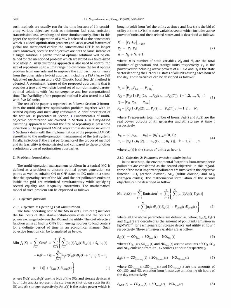
In this paper, a typical L.V MG is considered as the test systemfor application of suggested methodology. The proposed MGincludes various DG sources such as MT, a low temperature PAFC(Phosphoric Acid Fuel Cell), PV, WT (Wind Turbine) and a NiMH-Battery (Nickel-Metal-Hydride battery) as shown in Fig. 1. Theback-up MT/PAFC/NiMH-Battery hybrid power source is situatedat different locations in the MG, to level the mismatch betweenrenewable power generators and consumption and/or to store thesurplus of power from renewable sources for later use duringnon-generation or low power generation time periods. It isassumed that all DGs produce active power at unity power factor,neither requesting nor producing reactive power. Besides, allunits in this paper are assumed to be operating in electricitymode only and no heat is required for the examined period. Thereis also an electrical link for power exchange between the MG andthe utility during different hours of a day based on decisionsmade by MGCC.

4. Fundamentals of multi-objective optimization

Multi-objective optimization is a concept associated with manyreal-world optimization problems which aim at finding optimalsolutions considering different objectives simultaneously. Thesemulti-criteria optimization problems can not be handled throughfinding a single optimal solution, because a particular solution isn’tthe best with regard to all objectives. Therefore, a multi-objectiveoptimization problem leads to a set of optimal solutions knownas Pareto-optimal. Generally, in a multi-objective optimizationproblem there are different objective functions required to beoptimized simultaneously considering a set of equality andinequality constraints as follows [44,45]:

Minimize F ¼ ½f1ðXÞ; f2ðXÞ; .; fnðXÞ�T

Subject to :

�giðXÞ < 0 i ¼ 1;2.; NueqhiðXÞ ¼ 0 i ¼ 1;2.; Neq

(13)

where, F is a vector including objective functions and X is a vectorcontaining optimization variables, fi(X) is the ith objective function,gi(X) and hi(X) are the equality and inequality constraints respec-tively and n is the number of objective functions. For a multi-objective optimization problem, any two solutions X and Y canhave one of these two possibilities: one dominates the other ornone dominates the other. In a minimization problem, without lossof generality, a solution X dominates Y if the following two condi-tions are satisfied:

cj˛f1;2; .; ng; fjðXÞ � fjðYÞdk˛f1;2; .; ng; fkðXÞ < fkðYÞ (14)

Through the entire search space, the non-dominated solutionsare considered as “Pareto-optimal” and form the Pareto-optimal setor Pareto-optimal front. Likewise, “Pareto-dominance” is a conceptused for determining the eligibility of each particle (or solution) tobe stored in the repository of non-dominated solutions. A feasible

Fig. 1. A typical L.V micro-grid.


solution can be added to the repository if it satisfies any of thefollowing conditions [46]:

� The repository is full but the candidate solution is non-dominated and it is in a less crowded region than at least onesolution,

� The repository is not full and the candidate solution is notdominated by any solution in the repository,

� The candidate solution dominates all the solutions in therepository,

� The repository is empty.

Fig. 2. Fundamental elements for a particle displacement in PSO algorithm.

5. Fuzzy clustering for control the size of repository

It was mentioned earlier that in a multi-objective optimizationproblem, non-dominated solutions are stored in a predefinedrepository. Since the repository of non-dominated solutions hasa finite size, a limited number of candidate solutions can be storedand the rest should be omitted. Up to now, various techniquesbased on artificial intelligence have been proposed for controllingthe size of repository [47] and in this paper, a fuzzy-based clus-tering approach has been applied to do the same task. First, a fuzzymembership function is used to evaluate each objective functionrelated to any individual inside the repository as follows:

mfiðXÞ ¼

8>>><>>>:1; fiðXÞ � fmin

i0; fiðXÞ � fmax

ifmaxi � fiðXÞfmaxi � fmin

i

; fmini � fiðXÞ � fmax

i

(15)

where fimin and fimax are the lower and upper bounds of ith objective

function, respectively. In the proposed algorithm, the values of fimin

and fimax are evaluated by optimizing each objective function

separately. In the next step, the normalized membership value iscalculated for each element inside the repository, as follows:

NmðjÞ ¼Pn

k¼1 uk � mfk�Xj�

Pmj¼1

Pnk¼1 uk � mfk

�Xj� (16)

where m is the number of non-dominated solutions, uk is theweight factor for kth objective function. The normalized


membership value is a decisive criterion used for storing the bestnon-dominated solutions in the repository i.e., in a fuzzy clusteringapproach for control the size of repository, initially the normalizedmembership values are calculated and sorted, then, the best indi-viduals are selected and stored in the repository.

6. PSO algorithm

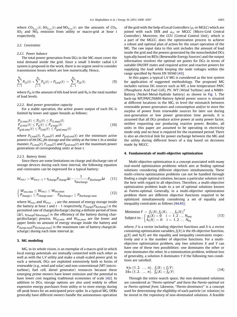
Among the evolutionary-based optimization algorithms, PSOhas been significantly used in multi-objective problems mainly dueto its population-based search capability as well as simplicity,convergence speed, and robustness. It was first introduced byKennedy and Eberhart [48] and was based on the imitation ofanimals’ social behaviors using tools and ideas taken fromcomputer graphics and social psychology research. Usually, PSOsimulates the behaviors of a flock of bird called “swarm” in whichany single and feasible solution is a bird and is called “particle”. Eachparticle has its own fitness value evaluated by the fitness function,and has a velocity vector which addresses the flying of the particle.To reach the optimal point, particles must update their nextdisplacements according to their own velocities, their best perfor-mances and the best performance of their best informant as shownin Fig. 2 and formulated as follows:

V ðkþ1Þi ¼ u� V ðkÞ

i þ C1 � rand1ð$Þ ��Pbest;i � XðkÞ

i

þ C2

� rand2ð$Þ ��Gbest � XðkÞ

i

(17)

Xðkþ1Þi ¼ XðkÞ

i þ V ðkþ1Þi (18)

where V ðkþ1Þi is the updated velocity vector of ith particle based on

the three displacement fundamentals, Xðkþ1Þi is the updated posi-

tion of ith particle, rand1($) and rand2($) denote two randomnumbers in the range [0,1] ، C1 and C2 are the learning factors and u

refers to inertia or momentum weight factor. Pbest,i is the bestprevious experience of ith particle that is recorded and Gbest is thebest particle (informant) among the entire population.

6.1. Binary PSO

To extend the real-valued PSO to discrete space where it isneeded, Kennedy and Eberhart calculate probability from thevelocity to determine whether Xðkþ1Þ

i will be in ON state or OFF (0/1). They squashed Vðkþ1Þ

i using the following logistic functions [49]:

r�V ðkþ1Þi

¼ 1

1þ exp�� V ðkþ1Þ

i

(19)

Xðkþ1Þi ¼

�1; if randð$Þ < r

�V ðkþ1Þi

0; otherwise

(20)

where rand($) is a uniform distribution in [0,1].

6.2. The proposed AMPSO approach

It was observed in the previous section that the performance ofa classic PSO algorithm depends greatly on three influentialparameters usually stated as the explorationeexploitation trade-off: learning factors (C1, C2) and momentum weight factor (u).Since a standard PSO algorithm along with a given set of param-eters is not capable of dealing with multi-objective optimizationproblems appropriately in all situations, some modifications arebecome necessary. In this paper, an adaptive modified PSO

algorithm is proposed in order to improve the performance ofa standard PSO approach and facilitate the multi-objective opti-mization process.

6.2.1. CLS mechanismTo enrich the search behavior and avoid the premature

phenomenon of PSO in solving multi-operation managementproblem, incorporating a chaotic search into PSO to constructa CPSO (chaotic PSO) is proposed. The chaotic search algorithm isdeveloped from the chaotic evolution of variables. Twowell-knownchaotic maps, logistic map and tent map, are the most commonmaps used in chaotic searches [50,51]. A rough description of chaosis that chaotic systems exhibit a great sensitivity to initial condi-tions. Due to the unique ergodicity characteristic, inherentstochastic property and irregularity of chaos, a chaotic can traverseevery state in a certain space by its own regularity and visit everystate once only, which helps avoid being trapped in local optima.Thus, a chaotic search has a much higher precision than some otherstochastic algorithms.

6.2.1.1. CLS type-1. The first CLSmechanism is an approachwhich isbased on the logistic map. The feature of the logistic map is thata small difference in the initial value of the chaotic variable wouldresult in a considerable difference in its long-time behaviors. Therelative simplicity of the logistic map makes it an excellent point ofentry into a consideration of the concept of chaos. Generallya logistic map is considered as follow:

Cxi ¼�cx1i ; cx

2i ; .; cxni

�1�n; i ¼ 0;1;2; .; Nchaos

cxjiþ1 ¼ 4� cxji ��1� cxji

; j ¼ 1;2; .; n

cxji˛½0;1�; cxj0;f0:25;0:5;0:75g

cxj0 ¼ randð$Þ

(21)

where, cxjiindicates the jth chaotic variable, Nchaos is the number ofindividuals for CLS, n is the number of DGs and rand($) is a randomnumber between 0 and 1. In this approach, first a particle is selectedrandomly from the repository (Xg) and considered as an initialpopulation for CLS ðX0

clsÞ. At the second step the initial population isscaled into [0,1] as follows:

X0cls ¼

hx1cls;0; x

2cls;0; .; xncls;0

i1�n

Cx0 ¼ �cx10; cx

20; .; cxn0

�

cxj0 ¼xjcls;0 � Pjmin;unit

Pjmax;unit � Pjmin;unit

; j ¼ 1;2; .; n

(22)

where Pjmin;unit and Pjmax;unit are the lower and upper limits of activepower for jth generation unit. The chaos population for CLS isgenerated as follows:

Xicls ¼

hx1cls;i;x

2cls;i; .; xncls;i

i1�n

i ¼ 1;2; .; Nchoas

xjcls;i ¼ cxji�1��Pjmax;unit�Pjmin;unit

þPjmin;unit; j ¼ 1;2; .; n

(23)

In the next step, the objective functions are calculated for anymember of the population and the non-dominated solutions arefound and sorted into a separate memory subsequently. The way inwhich one non-dominated solution is replaced with a particleselected randomly from the swarm is shown in Fig. 3.

Fig. 3. Chaotic Local Search (CLS) flowchart.


6.2.1.2. CLS type-2. The CLS type-2 is a procedure similar to the firstone but is based on the tent equation. In this mechanism thechaotic variables are defined as follows while the other instructionsremain unchanged.

Cxi ¼�cx1i ;cx

2i ;.; cxni

�1�n i¼ 0;1;2;.;Nchaos

cxjiþ1 ¼(

2cxji;

2�1�cxji

;

0<cxji�0:5

0:5< cxji�1j¼ 1;2;.; n

cxj0 ¼ randð$Þ

(24)

6.2.2. FSA mechanismIn a classic PSO approach the momentum weight factor (u) is

widely used both for controlling the scope of the search andreducing the importance of maximum velocity while the learningfactors (C1 and C2) are used for finding the optimum point throughconcentration on promising candidate solutions. In this regard, C1

has a contribution toward self-exploration of a particle while C2 hasa contribution toward motion of the particles in global directionconsidering themotion of all the particles in the preceding programiterations.

To overcome all the deficiencies associated with a conven-tional PSO algorithm, a FSAPSO (Fuzzy Self Adaptive PSO) mech-anism is developed to adjust the inertia weight and the learningfactors when they are needed. For this purpose, two triangularmembership functions are proposed; one for the learning factorsadjustment and the other for weight inertia tuning, as shown inFigs. 4 and 5. The input set for learning factors adjustment are thebest fitness (BF) and the number of generations for unchangedbest fitness (NU) while the best fitness (BF) and the inertia weight(u) are the input set for the second membership function. In thefirst membership function linguistic variables for inputs (NBF,NU) and outputs (C1, C2) are as following: Positive Small (PS),Positive Medium (PM), Positive Big (PB) and Positive Bigger (PR).Similarly, for the second membership function linguistic values

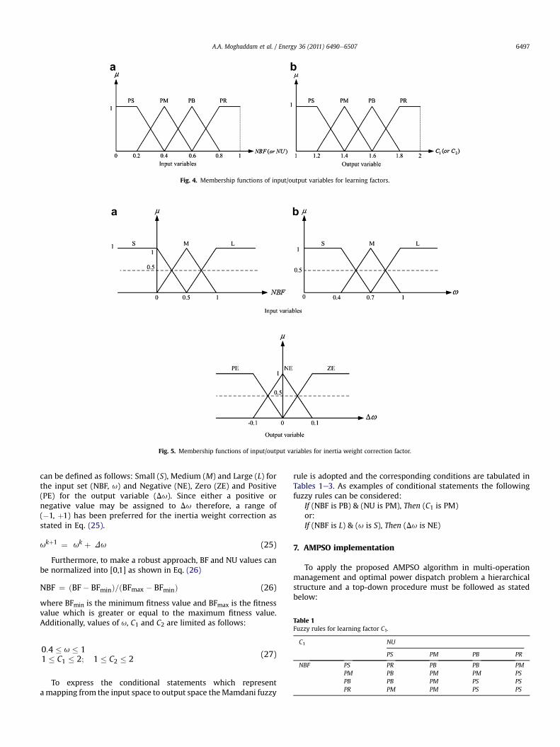
Table 1Fuzzy rules for learning factor C1.

C1 NU

PS PM PB PR

NBF PS PR PB PB PMPM PB PM PM PSPB PB PM PS PSPR PM PM PS PS

Fig. 4. Membership functions of input/output variables for learning factors.

Fig. 5. Membership functions of input/output variables for inertia weight correction factor.


can be defined as follows: Small (S), Medium (M) and Large (L) forthe input set (NBF, u) and Negative (NE), Zero (ZE) and Positive(PE) for the output variable (Du). Since either a positive ornegative value may be assigned to Du therefore, a range of(�1, þ1) has been preferred for the inertia weight correction asstated in Eq. (25).

ukþ1 ¼ uk þ Du (25)

Furthermore, to make a robust approach, BF and NU values canbe normalized into [0,1] as shown in Eq. (26)

NBF ¼ ðBF� BFminÞ=ðBFmax � BFminÞ (26)

where BFmin is the minimum fitness value and BFmax is the fitnessvalue which is greater or equal to the maximum fitness value.Additionally, values of u, C1 and C2 are limited as follows:

0:4 � u � 11 � C1 � 2; 1 � C2 � 2 (27)

To express the conditional statements which representamapping from the input space to output space theMamdani fuzzy

rule is adopted and the corresponding conditions are tabulated inTables 1e3. As examples of conditional statements the followingfuzzy rules can be considered:

If (NBF is PB) & (NU is PM), Then (C1 is PM)or:If (NBF is L) & (u is S), Then (Du is NE)

7. AMPSO implementation

To apply the proposed AMPSO algorithm in multi-operationmanagement and optimal power dispatch problem a hierarchicalstructure and a top-down procedure must be followed as statedbelow:

Table 2Fuzzy rules for learning factor C2.

C2 NU

PS PM PB PR

NBF PS PR PB PM PMPM PB PM PS PSPB PM PM PS PSPR PM PS PS PS


Step 1: Input data definitionAt the beginning of the program required input data must beprovided precisely. This information includes: MG configu-ration, operational characteristics of DGs and the utility,predicted output powers of WT and PV for a day ahead,hourly bids of DGs and the utility, emission coefficients ofmentioned units, objective functions and the MG daily loadcurve.

Step 2: Program initializationAt the second step the programmust be initialized by a set ofrandom populations and their corresponding velocities asfollows:

Population¼ �X1 X2 / XNswarm

�T� �

Fig. 6. Flowchart of power dispatch algorithm.

X0 ¼ x10;x20;.; xn0

xj0 ¼ randð$Þ��xmaxj �xmin

j

þxmin

j ; Xi ¼hxji

i1�n

j¼ 1;2;3;.; n; i¼ 1;2;.; Nswarm; n¼ 2��NgþNsþ1

�(28)

Velocity ¼ �V1 V2 / VNswarm

�TVi ¼ ½vi�1�n

vi ¼ randð$Þ � �vmaxi � vmin

i

�þ vmini ;

i ¼ 1;2;3; .; Nswarm; n ¼ 2� �Ng þ Ns þ 1

�(29)

where, n is the number of state variables, vi and xi are the velocityand position of the ith state variable respectively. rand($) isa random number between 0 and 1.

Step 3: do (i¼ 1)Step 4: Select the ith individual and calculate the values ofcorresponding objective functions

For the selected individual, the values of objective functionsare calculated separately using the dispatch algorithm illus-trated in Fig. 6.

Step 5: Store the ith individual in the repository if it is a non-dominated solution and apply the fuzzy clustering approachfor controlling the size of repository.Step 6: Find the local best solution for ith individual (Pbest,i)

At the beginning of the program, the initial generated pop-ulations are considered as local best solutions. During anyiteration of the program if one of the following criteria is

Table 3Fuzzy rules for inertia weight correction factor.

Du u

S M L

NBF S ZE NE NEM PE ZE NEL PE ZE NE

satisfied then the local best solutions are updated, otherwisethey remain unchanged:(i) If the former local best is dominated by the current one,

then the later is selected as the local best solution,(ii) If none of them dominates each other, the one with the

higher normalized membership function is consideredas the local best.

Step 7: i¼ iþ 1Step 8: While (i�Nswarm) redo steps 4e7Step 9: Select the global best (Gbest)

In this step, the global best solution is selected randomlyfrom the candidate solutions. To define Gbest value, first thenormalized membership values must be calculated for all ofthe non-dominated solutions inside the repository usingEq. (16)

Nm ¼ ½Nm1;Nm2; .; Nmi; .; Nmm�1�k (30)

where, Nmi is the normalized membership value for the ith non-
dominated solution and k is the size of repository. Afterward, thecumulative probabilities of the individuals are calculated asfollows:
Ci ¼ ½C1;C2; .; Cm�1�k8>><>>:

C1 ¼ Nm1C2 ¼ C1 þ Nm2«Ck ¼ Ck�1 þ Nmk

(31)

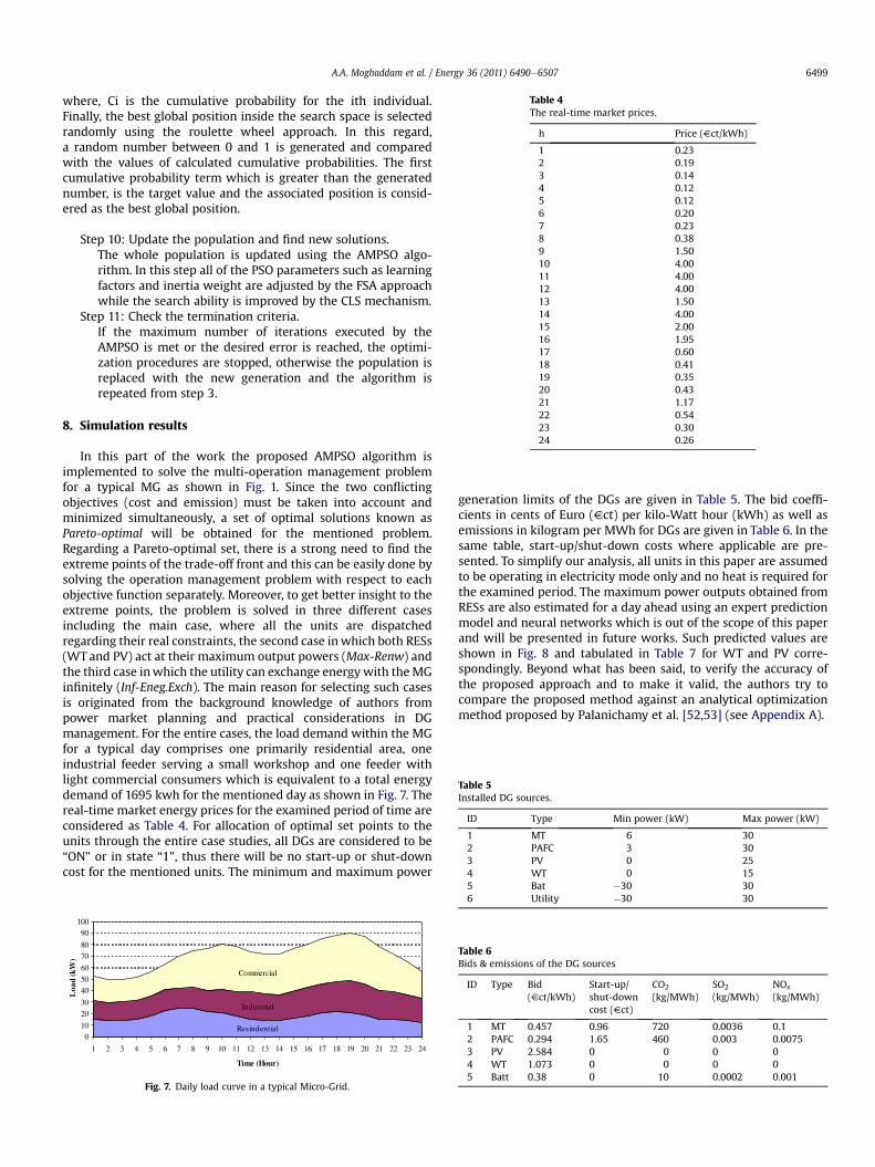
Table 5Installed DG sources.

ID Type Min power (kW) Max power (kW)

1 MT 6 302 PAFC 3 303 PV 0 254 WT 0 15

Table 4The real-time market prices.

h Price (Vct/kWh)

1 0.232 0.193 0.144 0.125 0.126 0.207 0.238 0.389 1.5010 4.0011 4.0012 4.0013 1.5014 4.0015 2.0016 1.9517 0.6018 0.4119 0.3520 0.4321 1.1722 0.5423 0.3024 0.26


where, Ci is the cumulative probability for the ith individual.Finally, the best global position inside the search space is selectedrandomly using the roulette wheel approach. In this regard,a random number between 0 and 1 is generated and comparedwith the values of calculated cumulative probabilities. The firstcumulative probability term which is greater than the generatednumber, is the target value and the associated position is consid-ered as the best global position.

Step 10: Update the population and find new solutions.The whole population is updated using the AMPSO algo-rithm. In this step all of the PSO parameters such as learningfactors and inertia weight are adjusted by the FSA approachwhile the search ability is improved by the CLS mechanism.

Step 11: Check the termination criteria.If the maximum number of iterations executed by theAMPSO is met or the desired error is reached, the optimi-zation procedures are stopped, otherwise the population isreplaced with the new generation and the algorithm isrepeated from step 3.

8. Simulation results

In this part of the work the proposed AMPSO algorithm isimplemented to solve the multi-operation management problemfor a typical MG as shown in Fig. 1. Since the two conflictingobjectives (cost and emission) must be taken into account andminimized simultaneously, a set of optimal solutions known asPareto-optimal will be obtained for the mentioned problem.Regarding a Pareto-optimal set, there is a strong need to find theextreme points of the trade-off front and this can be easily done bysolving the operation management problem with respect to eachobjective function separately. Moreover, to get better insight to theextreme points, the problem is solved in three different casesincluding the main case, where all the units are dispatchedregarding their real constraints, the second case inwhich both RESs(WT and PV) act at their maximum output powers (Max-Renw) andthe third case inwhich the utility can exchange energywith theMGinfinitely (Inf-Eneg.Exch). The main reason for selecting such casesis originated from the background knowledge of authors frompower market planning and practical considerations in DGmanagement. For the entire cases, the load demand within the MGfor a typical day comprises one primarily residential area, oneindustrial feeder serving a small workshop and one feeder withlight commercial consumers which is equivalent to a total energydemand of 1695 kwh for the mentioned day as shown in Fig. 7. Thereal-time market energy prices for the examined period of time areconsidered as Table 4. For allocation of optimal set points to theunits through the entire case studies, all DGs are considered to be“ON” or in state “1”, thus there will be no start-up or shut-downcost for the mentioned units. The minimum and maximum power

Resindential

Industrial

Commercial

010

2030

405060

7080

90100

1 2 3 4 5 6 7 8 9 10 11 12 13 14 15 16 17 18 19 20 21 22 23 24

Time (Hour)

Wk(dao

L)

Fig. 7. Daily load curve in a typical Micro-Grid.

generation limits of the DGs are given in Table 5. The bid coeffi-cients in cents of Euro (Vct) per kilo-Watt hour (kWh) as well asemissions in kilogram per MWh for DGs are given in Table 6. In thesame table, start-up/shut-down costs where applicable are pre-sented. To simplify our analysis, all units in this paper are assumedto be operating in electricity mode only and no heat is required forthe examined period. The maximum power outputs obtained fromRESs are also estimated for a day ahead using an expert predictionmodel and neural networks which is out of the scope of this paperand will be presented in future works. Such predicted values areshown in Fig. 8 and tabulated in Table 7 for WT and PV corre-spondingly. Beyond what has been said, to verify the accuracy ofthe proposed approach and to make it valid, the authors try tocompare the proposed method against an analytical optimizationmethod proposed by Palanichamy et al. [52,53] (see Appendix A).

5 Bat �30 306 Utility �30 30

Table 6Bids & emissions of the DG sources

ID Type Bid(Vct/kWh)

Start-up/shut-downcost (Vct)

CO2

(kg/MWh)SO2

(kg/MWh)NOx

(kg/MWh)

1 MT 0.457 0.96 720 0.0036 0.12 PAFC 0.294 1.65 460 0.003 0.00753 PV 2.584 0 0 0 04 WT 1.073 0 0 0 05 Batt 0.38 0 10 0.0002 0.001

Table 9Comparison of results in the case of emission objective for 20 trials (Main Case).

Type Best solution(kg)

Worst solution(kg)

Average(kg)

Standarddeviation (kg)

GA 435.2363 457.4680 445.3862 14.2299PSO 435.8227 454.5917 445.1072 13.9708FSAPSO 435.0830 451.3821 443.4396 11.3525CPSO-T 434.9973 444.9398 440.1036 6.9950CPSO-L 434.9354 443.6383 439.2369 6.1538AMPSO-T 434.8611 435.1126 434.9983 0.1786AMPSO-L 434.8193 435.0099 434.9235 0.0681

0

5

10

15

20

25

30

1 2 3 4 5 6 7 8 9 10 11 12 13 14 15 16 17 18 19 20 21 22 23 24

Time (Hour)

)Wk(t

uptuO

rewo

Pdeta

mitsE

WT PV

Fig. 8. Forecasted power outputs from RESs.

Table 7Forecasting output of WT & PV.

h WT (kW)/installed (kW) PV (kW)/installed (kW)

1 0.119 02 0.119 03 0.119 04 0.119 05 0.119 06 0.061 07 0.119 08 0.087 0.0089 0.119 0.15010 0.206 0.30111 0.585 0.41812 0.694 0.47813 0.261 0.95614 0.158 0.84215 0.119 0.31516 0.087 0.16917 0.119 0.02218 0.119 019 0.0868 020 0.119 021 0.0867 022 0.0867 023 0.061 024 0.041 0


8.1. First scenario (Main Case)

In the first scenario it’s assumed that all DGs with relatedcharacteristics produce electricity within the MG and additionaldemand or surplus of energy inside the grid is exchanged with theutility from the point of common coupling (PCC). All the unitsincluding the macro-gird (utility) can operate just within theirpower limits while satisfying the needed constraints. Performanceevaluation of several optimization algorithms along with their bestresults in the case of each objective is presented in Tables 8 and 9respectively.

Table 8Comparison of results in the case of cost objective for 20 trials (Main Case).

Type Best solution(Vct)

Worst solution(Vct)

Average(Vct)

Standarddeviation (Vct)


In these tables, all the evolutionary optimization methodsincluding the GA, PSO, FSAPSO, CPSO-T (Chaotic PSO based on Tentequation), CPSO-L (Chaotic PSO based on Logistic equation),AMPSO-L (Adaptive Modifies PSO based on Logistic equation) andAMPSO-T (Adaptive Modified PSO based on Tent equation) arecompared for 20 random trials for both objective functions. Forbetter understanding of the AMPSO performance, the convergencecharacteristics of AMPSO-L against the standard PSO algorithm forthe best solution and in the case of each objective are shown inFigs. 9 and 10 separately. Likewise, the best optimal power alloca-tions to the DGs using the proposed algorithm (AMPSO-L) are

Fig. 9. Convergence characteristics of AMPSO-L and PSO in the case of cost objective(main scenario).

Table 11Environmental power dispatch using AMPSO-L (Main Case: Totalemission¼ 434.8193 kg).

Time(h)

Units

MT (kW) FC (kW) PV (kW) WT (kW) Batt (kW) Utility (kW)

1 6.0024 30 0 1.78554 15 �0.78792 6 30 0 1.78554 30 �17.7853 6.0065 30 0 1.78554 30 �17.7924 6.0118 30 0 1.78554 30 �16.7975 6.0024 30 0 1.78554 29.9999 �11.7876 6 30 0 0.91324 29.9982 �3.91157 6 30 0 1.78554 30 2.214458 6 30 0.19374 1.30166 30 7.504599 6 29.9896 3.75395 1.78554 30 4.4709010 6 30 7.52793 3.08541 29.9999 3.3866711 6 30 10.4411 8.77236 30 �7.2135412 6 30 11.9640 10.4132 30 �14.377313 6 30 23.8929 3.92283 29.9999 �21.815814 6 30 21.0493 2.37655 29.9995 �17.425515 6 30 7.86474 1.78549 29.9989 0.3507816 6.0060 30 4.22076 1.30166 30 8.4715317 6 30 0.53879 1.78554 30 16.675618 6 30 0 1.78554 30 20.214419 6 30 0 1.30166 30 22.698320 6 30 0 1.78554 30 19.214421 6.0034 30 0 1.30166 29.9998 10.694922 6.0036 30 0 1.30166 30 3.6946923 6 30 0 0.91203 30 �1.9120324 6 30 0 0.61244 30 �10.6124

Table 10Economic power dispatch using AMPSO-L (Main Case: Total cost¼ 156.3628 Vct).

Time(h)

Units


1 6.0879 28.741 0 0 �10.553 27.72362 6 14.4023 0 0.0005 �0.1090 29.70623 6 15.4825 0 0 �1.4739 29.99154 6 12.545 0 0.0002 2.4548 305 6.1626 17.495 0 0 2.4661 29.87636 6.5555 29.1178 0 0 �2.6667 29.99347 6 22.3893 0 0 12.3333 29.27738 6.0292 29.5403 0 0 23.2481 16.18249 29.9836 29.9985 0.0168 1.7855 29.9792 �15.763710 30 30 7.4938 3.0815 29.9993 �20.574611 29.994 30 9.2913 8.707 30 �29.992312 30 30 3.5586 10.399 30 �29.957713 29.9803 30 0.0159 3.7738 30 �21.7714 29.9963 30 9.5516 2.3766 30 �29.924515 29.9998 29.9936 0.0871 1.7855 30 �15.86616 29.9981 29.98 0 1.2714 30 �11.249517 29.4817 29.9514 0.0052 0 29.978 �4.416418 6 29.9154 0 0.0199 29.8365 22.228219 6.0059 29.8798 0 0.0037 27.4502 26.660420 6 29.9901 0 0 29.9981 21.011821 30 30 0 1.2033 30 �13.203322 29.9616 29.6838 0 0.0049 29.9257 �18.57623 6.0031 14.6298 0 0 29.1347 15.232424 6.1143 4.8857 0 0 15 30

Fig. 10. Convergence characteristics of AMPSO-L and PSO in the case of emissionobjective (main scenario).


presented in Tables 10 and 11 regarding each objective functionminimization. Comparison of results in the case of best and worstsolutions for both objectives indicates that the proposed AMPSO-Lalgorithm not only demonstrates a better performance but alsopresents a faster convergence characteristic. Moreover, the statis-tical indices of average and standard deviation confirm anotheradvantage of the proposed algorithm in optimization process. It canbe also seen from Figs. 9 and 10 that the cost objective functionvalue reaches to minimum after 681 iterations with AMPSO-Lmethod and does not vary thereafter while the PSO algorithmconverges in 870 iterations. Similarly the value of emission objec-tive function settles to the minimum in 619 iterations with AMPSO-L method, while the PSO algorithm converges in 891 iterations.Besides, the numerical results of multi-objective operation ob-tained by the proposed AMPSO-L algorithm indicate that in the firsthours of the day a large portion of the load is supplied by the FCwithin the grid and the utility through the PCC because the bids ofcorresponding units are lower in comparison with those of othersduring the examined period. Due to growth of demand and bids ofutility during the next hours of the day DGs increase their outputpowers according to priority in lower cost and emission corre-spondingly. It should be also noted that the charging process of theNiMH-Battery is done at the first hours of the day when the pricesare low but the discharge action is postponed to the midday when

Table 12Comparison of results in the case of cost objective for 20 trials (Max-Renw).


Worst solution(Vct)

Average(Vct)



Table 13Comparison of results in the case of emission objective for 20 trials (Max-Renw).


Worst solution(kg)

Average(kg)



Table 14Economic power dispatch using AMPSO-L (Max-Renw: Total cost¼ 274.4317 Vct).

Time(h)

Units


1 6 28.8862 0 1.7855 �14.671 302 6 21.5035 0 1.7855 �9.2891 303 6 26.4814 0 1.7855 �14.266 304 6 29.993 0 1.7855 �16.778 305 6 26.6394 0 1.7855 �8.424 306 6 29.9993 0 0.9142 �3.913 307 6 23.4284 0 1.7855 8.7861 308 6 30 0.1937 1.3017 23.784 13.71989 30 30 3.754 1.7855 30 �19.539510 30 30 7.5279 3.0854 30 �20.613311 28.7865 29.9999 10.4412 8.7724 30 �3012 21.6227 30 11.964 10.4133 30 �3013 14.1839 29.9999 23.8934 3.9228 30 �3014 18.5741 30 21.0493 2.3766 30 �3015 30 30 7.8647 1.7855 30 �23.650316 30 30 4.2208 1.3017 30 �15.522417 30 30 0.5389 1.7855 30 �7.324418 6 30 0 1.7855 30 20.214519 6.0002 30 0 1.3017 29.999 22.698320 6 30 0 1.7855 30 19.214521 30 30 0 1.3017 30 �13.301722 28.6036 30 0 1.3017 30 �18.905223 6 30 0 0.9142 15.192 12.893524 6 18.2558 0 0.6124 1.1318 30

Table 15Comparison of results in the case of cost objective for 20 trials (Inf-Eneg.Exch).


Worst solution(Vct)

Average(Vct)



Table 17Economic power dispatch using AMPSO-L (Inf-Eneg.Exch: Total cost¼ 89.9720 Vct).

Time(h)

Units


1 6.0061 3.0023 0 0 �15 57.99162 6.0021 3.0065 0 0 �29.9672 70.95853 6.0069 3.0059 0 0 �30 70.98724 6 3.0005 0 0 �29.999 71.99855 6 3.008 0 0.0009 �30 76.99116 6 3.0404 0 0 �18.7679 72.72757 6 3 0 0 �4.1048 65.10488 6.0004 29.9869 0 0 10.8885 28.12429 29.9994 30 0 1.7855 25.8884 �11.673410 30 30 7.5279 3.0853 30 �20.613211 29.9998 30 10.4412 8.7723 29.9994 �31.212712 29.9997 30 11.9623 10.4133 29.9996 �38.374913 29.9998 30 0 3.9228 30 �21.922614 30 30 21.0493 2.3766 30 �41.425815 30 30 0.0001 1.7836 30 �15.783716 30 30 0.0024 1.3017 30 �11.304117 29.9877 29.9999 0 0 30 �4.987618 6.0157 29.9998 0 0 29.9818 22.002719 6.0059 29.9844 0 0 29.9974 24.012320 6.0027 29.9998 0 0.0037 29.9999 20.993821 30 30 0 1.2777 30 �13.277722 30 30 0 0 30 �1923 6 29.982 0 0 15 14.01824 6 3 0 0 0.1042 46.8958

Table 16Comparison of results in the case of emission objective for 20 trials (Inf-Eneg.Exch).


Worst solution(kg)

Average(kg)




the load curve reaches peak values. From another point of view,although employing RESs such as wind and solar results lesspollution inside the grid, it causes more cost in short-term opera-tion, therefore exploitation of energy form such resources must belimited according to economical considerations.

8.2. Second scenario (Max-Renw)

In the second scenario it’s assumed that RESs (WT & PV) areexploited at their available maximum power outputs during eachhour of the day and the rests of DGs including MT, PAFC, NiMH-Battery and the utility act as in the main case. Again, the entireoptimization schemes are applied to the optimization problemand corresponding results are recorded. Tables 12 and 13 show

Fig. 11. Comparison of Emission and Cost Pareto-optimal front of AMPSO-L, AMPSO-Tand PSO algorithms.

Fig. 13. Comparison of Emission and Cost Pareto-optimal front of all optimizationalgorithms.

Fig. 12. Comparison of Emission and Cost Pareto-optimal front of CPSO-L, CPSO-T,FSAPSO and PSO algorithms.


brief comparisons from the performances of the mentionedalgorithms regarding each objective for 20 trials. Similarly, theresult of economic power dispatch using the proposed approach isindicated in Table 14. It should be mentioned that the results ofenvironmental power dispatch don’t vary greatly among thescenarios mainly due to the fact that all RESs (which have thelowest emissions) are utilized up to their extremes during theexamined period.

Regarding the second scenario, it’s again observed that theproposed algorithm allocates optimal power set points to the DGsappropriately while keeping small diversity in finding the optimalsolutions during different trials in the case of each objective. It’salso investigated from Table 14 that the operating cost of the MGincreases greatly in comparison with the main case and demon-strates a growth of %75.5 in related cost. In other words, althoughhigher penetration of RESs into the grid environment results loweremission, it imposes higher cost of operation.

8.3. Third scenario (Inf-Eneg.Exch)

In the last scenario, it’s supposed that the utility behaves as anunconstraint unit and exchanges energy with the MG without anylimitation while the rests of DGs and their related characteristicsremain unchanged. Similar to the previous scenarios, all the opti-mization algorithms are implemented to solve the economicdispatch problem and the simulation results are gathered corre-spondingly as shown in Tables 15 and 16. The best performance ofAMPSO-L in scheduling of the units for a day ahead and in terms ofcost objective is also shown in Table 17. Once again, it’s observedthat the proposed algorithm can solve the optimization problemsuccessfully while maintains small variations in finding optimalsolutions considering both objectives. Moreover, the numericalresults of Table 17 indicate that allocation of optimal powers to DGsregarding an unlimited power exchange situation ends in a reduc-tion of %42.45 in operation cost of the MG in comparison with themain case. It’s also notable that in the third scenario the utility takesthe lead in supplying the load inside the grid during the first hoursof the day while purchasing energy in bulk amount from the MGduring the peak times. From an economical point of view, WT andPV start-up when shortage of power generation occurs inside thegrid or there is a need for more energy export to the macro-grid.Likewise, other DGs such as FC, MT and NiMH-Battery adjusttheir generation set points according to load levels during eachhour of the day in an economical manner.

Now to incorporate the availability of DGs in optimizationscheme while considering both objectives, suitable ON (OFF)states (0/1) are assigned to DGs during the power dispatchprocess. In such situation, all the units are allowed to start-up orshut-down for the flexible operation of the MG while consideringminimum cost and emission as competitive objectives. Again allthe evolutionary methods are implemented to solve the multi-operation management problem and related results as well asthe distribution of the Pareto-optimal sets over the trade-offsurfaces are gathered truthfully. The fuzzy-based clusteringprocedure is also utilized to control the size of repository duringthe optimization process. In this regard, the Pareto-fronts foremission and cost objectives obtained by PSO, AMPSO-L andAMPSO-T algorithms are shown in Fig. 11. The comparison ofPareto-fronts obtained by CPSO-T, CPSO-L, FSAPSO and PSO arealso illustrated in Fig. 12 respectively. Comparison of results inthe case of Pareto-fronts for emission and cost objectives ob-tained by AMPSO-L, CPSO-L, FSAPSO, PSO and GA is alsodemonstrated in Fig. 13. In the same figure, the extreme points onthe Pareto front obtained by the proposed algorithm are shownas examples of two non-dominated solutions with minimumemission-maximum cost and minimum cost-maximum emission,respectively. The schedules of multi-operation managementregarding each mentioned situation are tabulated in Tables 18and 19 separately.

It’s observed from Fig. 11 that the non-dominated solutionsachieved by the proposed AMPSO-L algorithms are well-distributed over the Pareto front although the one from standardPSO lacks this feature. Similarly, through comparison of resultsobtained by CPSO-T, CPSO-L, FSAPSO and PSO it’s concluded thathybrid PSO approaches (e.g., FSAPSO or CPSO) improve the capa-bility of a classic PSO in finding non-dominated solutions to a highextent although there are slight differences between their corre-sponding performances. It’s also important to mention that theperformances obtained by the AMPSO-L methods outweigh theones from other algorithms both in terms of non-dominatedsolutions and diversity of them along the Pareto front as shownin Fig. 13.

Table 18Multi-operation management using AMPSO-L (Minimum emission/maximum cost: Total cost¼ 637.9021 Vct, Total emission¼ 748.731 kg).

Time (h) DG Units

State Output power

MT FC PV WT Batt Utility MT (kW) FC (kW) PV (kW) WT (kW) Batt (kW) Utility (kW)

1 1 0 1 0 0 1 30 0 0 0 0 222 0 1 1 1 1 1 0 23.2516 0 1.2901 15 10.45823 0 1 1 1 1 0 0 24.4556 0 0.275 25.2694 04 1 1 0 1 1 1 12.7687 30 0 1.78554 30 �23.5545 1 0 0 1 1 1 30 0 0 0.36763 30 �4.36766 1 1 1 1 1 1 30 22.8931 0 0.20483 21.3122 �11.4107 0 1 1 1 1 1 0 30 0 0.43394 28.8520 10.71408 0 1 1 1 1 1 0 30 0.19375 1.30166 30 13.50469 0 1 0 1 1 1 0 30 0 1.78554 30 14.214510 1 1 0 1 1 1 30 30 0 3.08542 30 �13.08511 0 1 1 1 1 0 0 28.7865 10.4412 8.77237 30 012 1 1 0 1 1 1 9.2932 30 0 10.4133 30 �5.706513 1 0 1 1 1 1 21.3074 0 5.14984 1.04588 28.0076 16.489314 1 1 1 1 1 1 15.9401 30 14.7868 2.37656 30 �21.10315 1 0 0 0 1 1 16 0 0 0 30 3016 0 1 1 1 1 1 0 30 4.22077 1.30166 27.0698 17.407817 0 1 0 0 1 1 0 30 0 0 30 2518 1 0 1 1 1 1 30 0 0 1.78554 26.2145 3019 0 1 1 1 1 1 0 28.6983 0 1.3017 30 3020 0 1 1 0 1 1 0 27 0 0 30 3021 1 0 1 1 1 1 30 0 0 1.3017 28.8964 17.801922 1 1 0 1 1 0 30 14.8867 0 1.3017 24.8116 023 1 1 1 0 1 0 7.8492 27.1508 0 0 30 024 0 1 0 0 1 0 0 30 0 0 26 0

Table 19Multi-operation management using AMPSO-L (Minimum cost/maximum emission: Total cost¼ 559.4872 Vct, Total emission¼ 797.1101 kg).

Time (h) DG Units

State Output Power

MT FC PV WT Batt Utility MT (kW) FC (kW) PV (kW) WT (kW) Batt (kW) Utility (kW)

1 1 1 0 1 1 0 30 5.2144 0 1.7855 15 02 1 1 1 0 1 1 20.726 3 0 0 22.051 4.22253 1 0 0 1 1 0 29.7902 0 0 0.5660 19.6436 04 0 1 1 1 1 0 0 19.4532 0 1.7855 29.7612 05 1 0 1 0 1 0 26 0 0 0 30 06 1 1 0 1 1 0 17.8923 30 0 0.1077 15 07 1 1 1 1 1 1 30 3 0 1.7855 16.92362 18.29088 0 1 1 1 1 1 0 30 0.1247 1.3017 13.5735 309 1 1 0 1 1 0 30 17.2657 0 0.1607 28.5735 010 1 1 0 0 1 1 28.7951 30 0 0 21.2048 011 1 1 1 0 1 1 30 30 10.4411 0 30 �22.441212 1 1 1 0 1 1 30 30 11.9640 0 30 �27.96413 1 0 0 1 1 1 30 0 0 0.1287 30 11.871214 1 1 1 0 1 1 28.3006 30 5.6980 0 30 �21.998715 1 1 1 1 1 1 30 19.2424 0.0785 0.9922 25.6868 016 1 1 1 0 1 1 20.2427 29.5252 1.0080 0 11.1615 18.062317 1 1 1 1 0 1 30 30 0.5389 1.7855 0 22.675518 1 1 0 1 1 1 24.3746 30 0 1.7855 15 16.839719 1 1 1 1 0 1 28.6983 30 0 1.3017 0 3020 1 1 1 1 1 1 30 13.2532 0 0 15 28.746721 1 1 1 1 0 1 30 17.3224 0 0.6776 0 3022 1 0 1 1 1 1 30 0 0 0 15 2623 1 0 0 0 1 1 6 0 0 0 30 2924 1 1 1 0 1 1 6 21.4939 0 0 30 �1.4939


9. Conclusion

In this paper, an expert multi-objective Adaptive Modified PSO(AMPSO) optimization algorithm is proposed and implemented tosolve the multi-operation management problem in a typical MGwith RESs. A CLS approach is applied to find the best local solutionswithin the search space and a FSA mechanism is utilized to adjustPSO parameterswhen they are needed.Moreover, a fuzzy clusteringapproach is used to control the size of repository for non-dominated

solutions. To evaluate the performance of the proposed algorithmseveral test cases are introduced and the simulation results aregathered subsequently. The numerical results indicate that theproposed method not only demonstrates superior performancesbut also shows dynamic stability and excellent convergence of theswarms. The proposed method also yields a true and well-distributed set of Pareto-optimal solutions giving the systemoperators various options to select an appropriate power dispatchplan according to environmental or economical considerations.


Appendix A

To compare the performance of the proposed algorithm withsome analytical methods a test system with three plants and sixgenerating units is considered as shown in Fig. A.1. The fuel costs

Fig. A.1. A Typical 4-bus test system

Fig. A.2. Pareto-fronts of AMPSO algorithm for the test system.

and the emission coefficients of corresponding units are tabulatedin Tables A.1eA.2. For simplicity, only one type of pollutant (NOx) isconsidered for optimization process. The transmission loss coeffi-cients are also shown in (A.1). More information on related testsystem is given in Ref. [52].

with six generation units [52].

Table A.2Emission coefficients (NOx).

Plant Unit Fuel cost coefficients PG,min (MW) PG,max (MW)

di ei fi

1 G1 0.00419 0.32767 13.85932 10 125G2 0.00419 0.32767 13.85932 10 150G3 0.00683 �0.54551 40.2669 40 250

2 G4 0.00683 �0.54551 40.2669 35 210G5 0.00461 �0.51116 42.89553 130 325

3 G6 0. 00461 �0.51116 42.89553 125 315

Table A.1Fuel cost coefficients.

Plant Unit Fuel cost coefficients PG,min (MW) PG,max (MW)

ai bi ci

1 G1 0.15274 38.53973 756.79886 10 125G2 0.10578 46.15916 451.32513 10 150G3 0.02803 40.39655 1049.32513 40 250

2 G4 0.03546 38.30553 1243.5311 35 210G5 0.02111 36.32782 1658.5696 130 325

3 G6 0.01799 38.27041 1356.65920 125 315

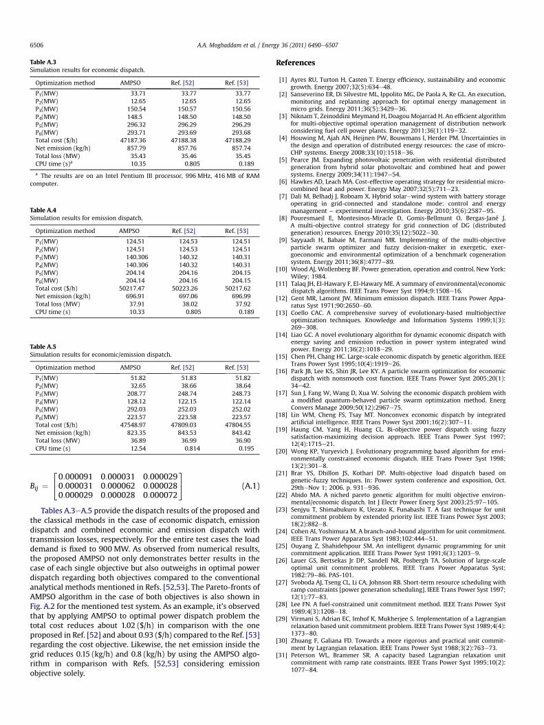
Table A.3Simulation results for economic dispatch.

Optimization method AMPSO Ref. [52] Ref. [53]

P1(MW) 33.71 33.77 33.77P2(MW) 12.65 12.65 12.65P3(MW) 150.54 150.57 150.56P4(MW) 148.5 148.50 148.50P5(MW) 296.32 296.29 296.29P6(MW) 293.71 293.69 293.68Total cost ($/h) 47187.36 47188.38 47188.29Net emission (kg/h) 857.79 857.76 857.74Total loss (MW) 35.43 35.46 35.45CPU time (s)a 10.35 0.805 0.189

a The results are on an Intel Pentium III processor, 996 MHz, 416 MB of RAMcomputer.

Table A.4Simulation results for emission dispatch.


P1(MW) 124.51 124.53 124.51P2(MW) 124.51 124.53 124.51P3(MW) 140.306 140.32 140.31P4(MW) 140.306 140.32 140.31P5(MW) 204.14 204.16 204.15P6(MW) 204.14 204.16 204.15Total cost ($/h) 50217.47 50223.26 50217.62Net emission (kg/h) 696.91 697.06 696.99Total loss (MW) 37.91 38.02 37.92CPU time (s) 10.33 0.805 0.189

Table A.5Simulation results for economic/emission dispatch.


P1(MW) 51.82 51.83 51.82P2(MW) 32.65 38.66 38.64P3(MW) 208.77 248.74 248.73P4(MW) 128.12 122.15 122.14P5(MW) 292.03 252.03 252.02P6(MW) 223.57 223.58 223.57Total cost ($/h) 47548.97 47809.03 47804.55Net emission (kg/h) 823.35 843.53 843.42Total loss (MW) 36.89 36.99 36.90CPU time (s) 12.54 0.814 0.195


Bij ¼240:000091 0:000031 0:0000290:000031 0:000062 0:0000280:000029 0:000028 0:000072

35 (A.1)

Tables A.3eA.5 provide the dispatch results of the proposed andthe classical methods in the case of economic dispatch, emissiondispatch and combined economic and emission dispatch withtransmission losses, respectively. For the entire test cases the loaddemand is fixed to 900 MW. As observed from numerical results,the proposed AMPSO not only demonstrates better results in thecase of each single objective but also outweighs in optimal powerdispatch regarding both objectives compared to the conventionalanalytical methods mentioned in Refs. [52,53]. The Pareto-fronts ofAMPSO algorithm in the case of both objectives is also shown inFig. A.2 for the mentioned test system. As an example, it’s observedthat by applying AMPSO to optimal power dispatch problem thetotal cost reduces about 1.02 ($/h) in comparison with the oneproposed in Ref. [52] and about 0.93 ($/h) compared to the Ref. [53]regarding the cost objective. Likewise, the net emission inside thegrid reduces 0.15 (kg/h) and 0.8 (kg/h) by using the AMPSO algo-rithm in comparison with Refs. [52,53] considering emissionobjective solely.

References

[1] Ayres RU, Turton H, Casten T. Energy efficiency, sustainability and economicgrowth. Energy 2007;32(5):634e48.

[2] Sanseverino ER, Di Silvestre ML, Ippolito MG, De Paola A, Re GL. An execution,monitoring and replanning approach for optimal energy management inmicro grids. Energy 2011;36(5):3429e36.

[3] Niknam T, Zeinoddini Meymand H, Doagou Mojarrad H. An efficient algorithmfor multi-objective optimal operation management of distribution networkconsidering fuel cell power plants. Energy 2011;36(1):119e32.

[4] Houwing M, Ajah AN, Heijnen PW, Bouwmans I, Herder PM. Uncertainties inthe design and operation of distributed energy resources: the case of micro-CHP systems. Energy 2008;33(10):1518e36.

[5] Pearce JM. Expanding photovoltaic penetration with residential distributedgeneration from hybrid solar photovoltaic and combined heat and powersystems. Energy 2009;34(11):1947e54.

[6] Hawkes AD, Leach MA. Cost-effective operating strategy for residential micro-combined heat and power. Energy May 2007;32(5):711e23.

[7] Dali M, Belhadj J, Roboam X. Hybrid solarewind system with battery storageoperating in grid-connected and standalone mode: control and energymanagement e experimental investigation. Energy 2010;35(6):2587e95.

[8] Pouresmaeil E, Montesinos-Miracle D, Gomis-Bellmunt O, Bergas-Jané J.A multi-objective control strategy for grid connection of DG (distributedgeneration) resources. Energy 2010;35(12):5022e30.

[9] Sayyaadi H, Babaie M, Farmani MR. Implementing of the multi-objectiveparticle swarm optimizer and fuzzy decision-maker in exergetic, exer-goeconomic and environmental optimization of a benchmark cogenerationsystem. Energy 2011;36(8):4777e89.

[10] Wood AJ, Wollenberg BF. Power generation, operation and control. New York:Wiley; 1984.

[11] Talaq JH, El-Hawary F, El-Hawary ME. A summary of environmental/economicdispatch algorithms. IEEE Trans Power Syst 1994;9:1508e16.

[12] Gent MR, Lamont JW. Minimum emission dispatch. IEEE Trans Power Appa-ratus Syst 1971;90:2650e60.

[13] Coello CAC. A comprehensive survey of evolutionary-based multiobjectiveoptimization techniques. Knowledge and Information Systems 1999;1(3):269e308.

[14] Liao GC. A novel evolutionary algorithm for dynamic economic dispatch withenergy saving and emission reduction in power system integrated windpower. Energy 2011;36(2):1018e29.

[15] Chen PH, Chang HC. Large-scale economic dispatch by genetic algorithm. IEEETrans Power Syst 1995;10(4):1919e26.

[16] Park JB, Lee KS, Shin JR, Lee KY. A particle swarm optimization for economicdispatch with nonsmooth cost function. IEEE Trans Power Syst 2005;20(1):34e42.

[17] Sun J, Fang W, Wang D, Xua W. Solving the economic dispatch problem witha modified quantum-behaved particle swarm optimization method. EnergConvers Manage 2009;50(12):2967e75.

[18] Lin WM, Cheng FS, Tsay MT. Nonconvex economic dispatch by integratedartificial intelligence. IEEE Trans Power Syst 2001;16(2):307e11.

[19] Haung CM, Yang H, Huang CL. Bi-objective power dispatch using fuzzysatisfaction-maximizing decision approach. IEEE Trans Power Syst 1997;12(4):1715e21.

[20] Wong KP, Yuryevich J. Evolutionary programming based algorithm for envi-ronmentally constrained economic dispatch. IEEE Trans Power Syst 1998;13(2):301e8.

[21] Brar YS, Dhillon JS, Kothari DP. Multi-objective load dispatch based ongenetic-fuzzy techniques. In: Power system conference and exposition, Oct.29theNov 1; 2006. p. 931e936.

[22] Abido MA. A niched pareto genetic algorithm for multi objective environ-mental/economic dispatch. Int J Electr Power Energ Syst 2003;25:97e105.

[23] Senjyu T, Shimabukuro K, Uezato K, Funabashi T. A fast technique for unitcommitment problem by extended priority list. IEEE Trans Power Syst 2003;18(2):882e8.

[24] Cohen AI, Yoshimura M. A branch-and-bound algorithm for unit commitment.IEEE Trans Power Apparatus Syst 1983;102:444e51.

[25] Ouyang Z, Shahidehpour SM. An intelligent dynamic programming for unitcommitment application. IEEE Trans Power Syst 1991;6(3):1203e9.

[26] Lauer GS, Bertsekas Jr DP, Sandell NR, Posbergh TA. Solution of large-scaleoptimal unit commitment problems. IEEE Trans Power Apparatus Syst;1982:79e86. PAS-101.

[27] Svoboda AJ, Tseng CL, Li CA, Johnson RB. Short-term resource scheduling withramp constraints [power generation scheduling]. IEEE Trans Power Syst 1997;12(1):77e83.

[28] Lee FN. A fuel-constrained unit commitment method. IEEE Trans Power Syst1989;4(3):1208e18.

[29] Virmani S, Adrian EC, Imhof K, Mukherjee S. Implementation of a Lagrangianrelaxation based unit commitment problem. IEEE Trans Power Syst 1989;4(4):1373e80.

[30] Zhuang F, Galiana FD. Towards a more rigorous and practical unit commit-ment by Lagrangian relaxation. IEEE Trans Power Syst 1988;3(2):763e73.

[31] Peterson WL, Brammer SR. A capacity based Lagrangian relaxation unitcommitment with ramp rate constraints. IEEE Trans Power Syst 1995;10(2):1077e84.


[32] Damousis IG, Bakirtzis AG, Dokopoulos PS. A solution to the unit-commitmentproblem using integer-coded genetic algorithm. IEEE Trans Power Syst 2004;19(2):1165e72.

[33] Senjyu T, Saber AY, Miyagi T, Shimabukuro K, Urasaki N, Funabashi T. Fasttechnique for unit commitment by genetic algorithm based on unit clustering.IEE Proc Generat Transmission Distrib 2005;152(5):705e13.

[34] Cheng CP, Liu CW, Liu CC. Unit commitment by Lagrangian relaxation andgenetic algorithms. IEEE Trans Power Syst 2000;15(2):707e14.

[35] Kazarlis SA, Bakirtzis AG, Petridis V. A genetic algorithm solution to the unitcommitment problem. IEEE Trans Power Syst 1996;11(1):83e92.

[36] Kennedy J, Eberhart R. Particle swarm optimization. In: Proc. IEEE Int. Conf.Neural Networks (ICNN’95), vol. 4; 1995.

[37] Coello CA, Lechuga Mopso MS. A proposal for multi objective particle swarmoptimization. In: Proceedings of IEEE world congress on computationalintelligence; 2002. p. 1051e1056.

[38] Deb K, Thiele L, Laumanns M, Zitzler E. Scable multi-objective optimizationtest problems, In: Proceeding of IEEE world congress on computationalintelligence (CEC2002); 2002.

[39] Fieldsend JE, Singh S. A multi objective algorithm based upon particle swarmoptimization an efficient data structure on turbulence. In the 2002 U.K.workshop on computational Intelligence;2002. p. 34e44.

[40] Hu Eberhart X. Multi-objective optimization using dynamic nighbourhoodparticle swarm optimization. In: Proceedings of IEEE world congress oncomputational intelligence; 2002. p. 1677e1681.

[41] Mostaghim S, Teich J. Strategies for finding good local guides in multi-objective particle swarm optimization. In: Proc. of IEEE swarm intelligencesymposium; 2003. p. 26e33.

[42] Hernandez-Aramburo CA, Green TC, Mugniot N. Fuel consumption minimi-zation of a microgrid. IEEE Trans Ind Appl 2005;41(3).

[43] Conti S, Rizzo SA. Optimal control to minimize operating costs and emissionsof MV autonomous micro-grids with renewable energy sources, Clean Elec-trical Power ICCEP’09; 2009. p. 634e639.

[44] Lin CM, Gen M. Multi-criteria human resource allocation for solving multi-stage combinatorial optimization problems using multiobjective hybridgenetic algorithm. Expert Syst Appl 2008;34:2480e90.

[45] Chang PC, Chen SH, Liu CH. Sub-population genetic algorithm with mininggene structures for multiobjective flowshop scheduling problems. Expert SystAppl 2007;33:762e71.

[46] Wang L, Singh Ch. Environmental/economic power dispatch using fuzzifiedmulti-objective particle swarm optimization algorithm. Electr Power Syst Res2007;77:1654e64.

[47] Kalogirou SA. Artificial intelligence for the modeling and control ofcombustion processes: a review. Progr Energ Combust Sci 2003;29:515e66.

[48] Kennedy J, Eberhart R. Particle swarm optimization. In: IEEE internationalconf. on neural networks. Piscataway, NJ, vol. 4; 1995. p. 1942e1948.

[49] Kennedy J, Eberhart RC. A discrete binary version of the particle swarmalgorithm. In: Proc. IEEE conf. on systems, man, and cybernetics; 1997. p.4104e4109.

[50] Liu B, Wang L, Jin YH, Tang F, Huang DX. Improved particle swarmoptimization combined with chaos. Chaos Solitons Fractals 2005;25(5):1261e71.

[51] Coelho LDS. A quantum particle swarm optimizer with chaotic mutationoperator. Chaos Solitons Fractals 2008;37(5):1409e18.

[52] Palanichamy C, Srikrishna K. Economic thermal power dispatch with emissionconstraint. J Indian Inst Eng (India) 1991;72(11).

[53] Palanichamy C, Babu NS. Analytical solution for combined economic andemissions dispatch. Electr Power Syst Res 2008;78(7):1129e39.

Multi-objective operation management of a renewable MG ... · Multi-objective operation management...

Documents

Transcript of Multi-objective operation management of a renewable MG ... · Multi-objective operation management...