Multi-Niche Crowding in Genetic Algorithms and its Application to theAssembly of DNA Restriction-Fragments

Walter Cedeño, V. Rao Vemuri, and Tom SlezakDepartment of Applied Science

University of California, Davis andLawrence Livermore National Laboratory

Livermore, CA 94550(wcedeno@llnl.gov, vemur1@llnl.gov and slezak1@llnl.gov)

Abstract

The determination of the sequence of all nucleotide base-pairs in a DNA molecule,

from restriction-fragment data, is a complex task and can be posed as the problem of

finding the optima of a multi-modal function. A genetic algorithm that uses multi-niche

crowding permits us to do this. Performance of this algorithm is first tested using a

standard suite of test functions. The algorithm is next tested using two data sets

obtained from the Human Genome Project at the Lawrence Livermore National

Laboratory. The new method holds promise in automating the sequencing

computations.

Key words: Genetic algorithms, multi-modal functions, DNA restriction fragment

assembly, human genome project;

2

1 Introduction

This paper describes how the concept of multi-niche crowding in a genetic algortihm

permits one to simultaneously find several extrema of a multi-modal function.

Although a complete theoretical analysis supported by performance data on the

method is still being worked out, initial results from experiments with a standard suite

of test functions are persuasive about the utility of this method to solve problems of

practical interest. The method is tested by applying it to solve a problem in molecular

biology, believed to be NP-hard.

Section 2 of this paper describes multi-modal function optimization using the new

GA model. The validity of the new method is demonstrated in Section 3 by applying it

on several multi-modal test functions. Section 4.1 gives a tutorial background on the the

Human Genome Project and the relevance of the restriction-fragment assembly

problem. Section 4.2 summarizes the experimental procedure used by one group of

biologists to gather the data used in this paper. Section 4.3 summarizes some of the

related work on restriction fragment map assembly. Section 5 addresses the

representational issues including a description of the genetic operators and the fitness

function used to solve this problem. Section 6 includes results and discussion and

Section 7 summarizes on-going work.

Because genetic algorithms are being used in this paper to solve a problem in

genetics, a word of caution about the terminology used is in order. Words like

"chromosomes" occur while describing the genetic algorithm as well as during the

description of the DNA fragment assembly process. To the biologist, a chromosome is

DNA. To the computational scientist, a chromosome is a data structure. The context will

make the intent abundantly clear.

3

2. Genetic Algorithms for Multi-modal Search

Searching for extrema in a multi-modal search space is different from locating the

extremum of a unimodal function. When a search technique proven to be useful for

unimodal functions is applied to multi-modal functions, the method tends to converge

to an optimum in the local neighborhood of the first guess. One can use ideas like

simulated annealing to escape from a local optimum. However, there are many

applications where the location of "k best extrema" of a multi-modal function are of

interest. Searching for these locations goes by the name "multi-modal optimization."

There are many versions of genetic algorithms, one differing from another in some

detail. For the purposes of this paper, it is sufficient to focus on two basic steps common

to all genetic algorithms. During the selection step, a decision is made as to who is

allowed to produce offspring, and during the replacement step another decision is made

as to which of the members from generation i are forced to perish (or vacate a slot) in

order to make room for an offspring.

The Simple GA (or, SGA) (Holland 1975), which will be used as a point of departure

for presenting our method, starts by randomly generating a population of N

individuals, that is individual solutions. These individuals are evaluated for their

fitness. Individuals with higher fitness scores are selected, with replacement, to create a

mating pool of size N. This method of selection is called fitness proportionate reproduction

(FPR). The genetic operators of crossover and mutation are applied at this stage in a

probabilistic manner which results in some individuals from the mating pool to

reproduce. The assumption here is that each pair of parents produce only one pair of

offspring through the crossover operation. That is, the second generation is comprised

of those first generation individuals who never got a chance to reproduce and the

offspring of those who got a chance to reproduce. The procedure continues until a

suitable termination condition is satisfied, say a specified number of generations. (For

the purposes of this paper, a generation is every N /2 mating operations, where N is the

4

population size.) All other versions of GAs differ from this basic method in some detail

or another.

The steady state GA (or, SSGA) (Whitley 1988; Syswerda 1989), differs from SGA

mainly in the replacement step, and to a lesser extent on the way the genetic operators

are applied. The SSGA selects two individuals using FPR and allows them to mate to

produce two offspring. This selection step is identical to the corresponding step of SGA.

However, in SSGA, the offspring are inserted into the population, thus replacing two

individuals, soon after they are generated. The SGA, on the other hand, generates N

offspring prior to replacing the entire population. In other words SGA uses simultaneous

replacement strategy whereas the SSGA uses the successive replacement strategy. Thus

SGA and SSGA are analogous, respectively, to the Jacobi and Gauss-Seidal methods of

solving systems of algebraic equations.

Both SGA and SSGA suffer from the possibility of premature convergence to a local

minimum, primarily due to the selection pressure exerted by the FPR rule. Simply

assigning an exponential number of mating opportunities to those members of the

population that exhibit above average survival traits, as the FPR rule does, is not a good

strategy for a thorough exploration of complex search spaces with multiple peaks. Due

to this reason as well as the deceptiveness exhibited by multi-modal search spaces

(Goldberg et al., 1992), SGA and SSGA are not suitable for multi-modal search and

optimization.

2.1 Multi-modal Search: Crowding-based Methods

The GA model described in this paper, called multi-niche crowding (or, MNC), has the

ability to converge simultaneously to multiple solutions by encouraging competition

between individuals within the same locally optimal group (Cedeño and Vemuri, 1992).

In MNC, both the selection and replacement steps of the SGA are modified with the

introduction of some form of crowding in order to render it suitable for searching spaces

5

characterized by multiple peaks or niches. For completeness, the concept of crowding is

briefly reviewed here.

Crowding (De Jong, 1975) is a generalization of preselection (Cavicchio, 1970). In

crowding, selection and reproduction are the same as in the SGA; but replacement is

different. For concreteness, it is assumed that two parents are selected to produce two

offspring. In order to make room for these offspring, it is necessary to identify two

members of the population for replacement. The policy of replacing a member of the

present generation by an offspring is carried out as follows, in two steps. First, a group

of C individuals is selected at random from the population. C, called the crowding factor,

also indicates the size of the group. A value of C = 2 or 3 appears to work well for De

Jong. Second, the bit strings in the offspring chromosomes are compared with those of

the C individuals in the group using Hamming distance as a measure of similarity. The

group member that is most similar to the offspring is now replaced by the offspring.

This procedure is repeated for the other offspring as well. This second offspring can

conceivably replace its own sibling that just entered the population pool, although such

a scenario is rather unlikely. In any event, crowding is essentially a successive

replacement strategy. This strategy maintains the diversity in the population and

postpones premature convergence. However crowding cannot maintain stable

subpopulations too long due to the selection pressure imparted by FPR. Summarizing,

in crowding offspring replace similar individuals from the population. Crowding slows

down premature convergence of the traditional GA and in most cases can find the

global optimum in a multi-modal search space. On the other hand it does not facilitate

convergence to multiple solutions and after many generations one of the peaks takes

over.

In deterministic crowding (Mahfound, 1992) selection pressure is eliminated and

preselection is introduced to obtain a very fast GA suitable for multi-modal function

6

optimization. In this method selection pressure is eliminated by allowing individuals to

mate at random with any other individual in the population. Pressure is applied,

however, during replacement step using preselection. Toward this goal, each of the two

offspring is first paired with one of the parents; this pairing is not done randomly,

rather the pairings are done in such a manner the offspring is paired with the most

similar parent. Then each offspring is compared with its paired parent and the

individual with the higher fitness is allowed to stay in the population and the other is

eliminated. It is not clear if multiple solutions can be maintained for many generations

using this method, although it appears that multiple solutions are sustained for more

generations than when crowding is used alone.

2.2 Multi-modal Search: Multi-niche Crowding

In multi-niche crowding (MNC), both the selection and replacement steps are

modified with some type of crowding. The idea is to eliminate the selection pressure

caused by FPR while allowing the population to maintain some diversity. This objective

is achieved, in part, by encouraging mating and replacement within members of the

same niche while allowing for some competition for population slots among the niches.

The result is an algorithm that (a) maintains stable subpopulations within different

niches, (b) maintains diversity throughout the search, and (c) converges to different

local optima.

In MNC, the FPR selection is replaced by what we call crowding selection. In

crowding selection, each individual in the population has the same chance for mating in

every generation. Application of this selection rule takes place in two steps. First, an

individual A is selected for mating. This selection can be either sequential or random.

Second, its mate M is selected, not from the entire population, but from a group of

individuals of size Cs, picked at random (with replacement) from the population. The

mate M thus chosen must be the one who is the most "similar" to A. The similarity

7

metric used here is not a genotypic metric such as the Hamming distance, but a suitably

defined phenotypic distance metric. Crowding selection promotes mating between

individuals from the same niche while allowing matings between individuals from

different niches.

During the replacement step, MNC uses a replacement policy called worst among the

most similar. The goal of this step is to pick an individual from the population for

replacement by an offspring. Implementation of this policy follows these steps. First, Cf

groups are created by randomly picking s individuals (with replacement) per group

from the population. These groups are called crowding factor groups. Second, one

individual from each group that is most phenotypically similar to the offspring is

identified. This gives Cf individuals that are candidates for replacement by virtue of

their similarity to the offspring that will replace them. From this group of most similar

individuals, we pick the one with the lowest fitness to die and that slot is filled with the

offspring. The offspring could possibly have a lower fitness than the individual being

replaced.

Both selection and replacement steps in the MNC are primarily based on a similarity

metric. Fitness is also considered during replacement to promote competition between

members of the same niche. Competition between members of different niches occurs as

well. The following pseudo-code summarizes the salient features of the MNC:

1. Generate initial population of N individuals2. For gen = 1 to MAX_GEN3. For i = 1 to N4. Use crowding selection to find mate for parent i5. Mate and mutate6. Insert offspring in the population using worst among most similar replacement.

If FPR is used in Step 4 above and if the individual with the lowest fitness in the

population (Step 6) is replaced with the newly generated offspring, this model

corresponds to a steady-state GA. In contrast with the most common generational GA,

8

offspring are available for mating as soon as they are generated, and good individuals

can survive for many generations. A similar technique called enhanced crowding

(Goldberg, 1989) has been used before in classifier systems, but there the most similar

individual out of a group of worst candidates is replaced. A pictorial interpretation of

the MNC replacement policy is shown in Figure 1.

...

Population

Randomly formcrowding factor(Cf ) groups

Group 1 withs individuals

Individual 1

Offspring

Lowest fittedindividual

Most similarto offspring

Group Cf withs individuals

Individual Cf

......

Replaces

Figure 1: Schematic showing worst among most similar replacement policy.

In summary, MNC differs from the other crowding based methods in the following

salient features:

(a) Both selection and replacement use a form of crowding.

(b) Mating among members of the same niche is encouraged.

(c) Competition among members of the same niche is promoted.

These features appear to be responsible for the apparantly superior performance of this

method over other crowding based methods insofar as maintaining solutions in

multiple peaks. The next section shows some performance results when this method is

applied to some standard test functions.

9

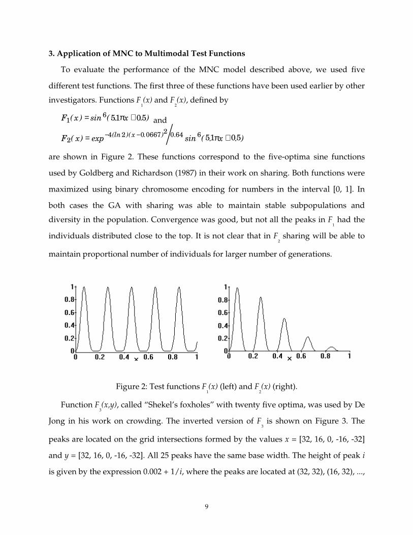
3. Application of MNC to Multimodal Test Functions

To evaluate the performance of the MNC model described above, we used five

different test functions. The first three of these functions have been used earlier by other

investigators. Functions F1(x) and F

2(x), defined by

F x x16 51 05( ) sin ( . . )= +π and

F x xx2

4 2 0 0667 2 0 64 6 51 05( ) exp sin ( . . )(ln )( . ) .= +− − π

are shown in Figure 2. These functions correspond to the five-optima sine functions

used by Goldberg and Richardson (1987) in their work on sharing. Both functions were

maximized using binary chromosome encoding for numbers in the interval [0, 1]. In

both cases the GA with sharing was able to maintain stable subpopulations and

diversity in the population. Convergence was good, but not all the peaks in F1 had the

individuals distributed close to the top. It is not clear that in F2 sharing will be able to

maintain proportional number of individuals for larger number of generations.

Figure 2: Test functions F1(x) (left) and F

2(x) (right).

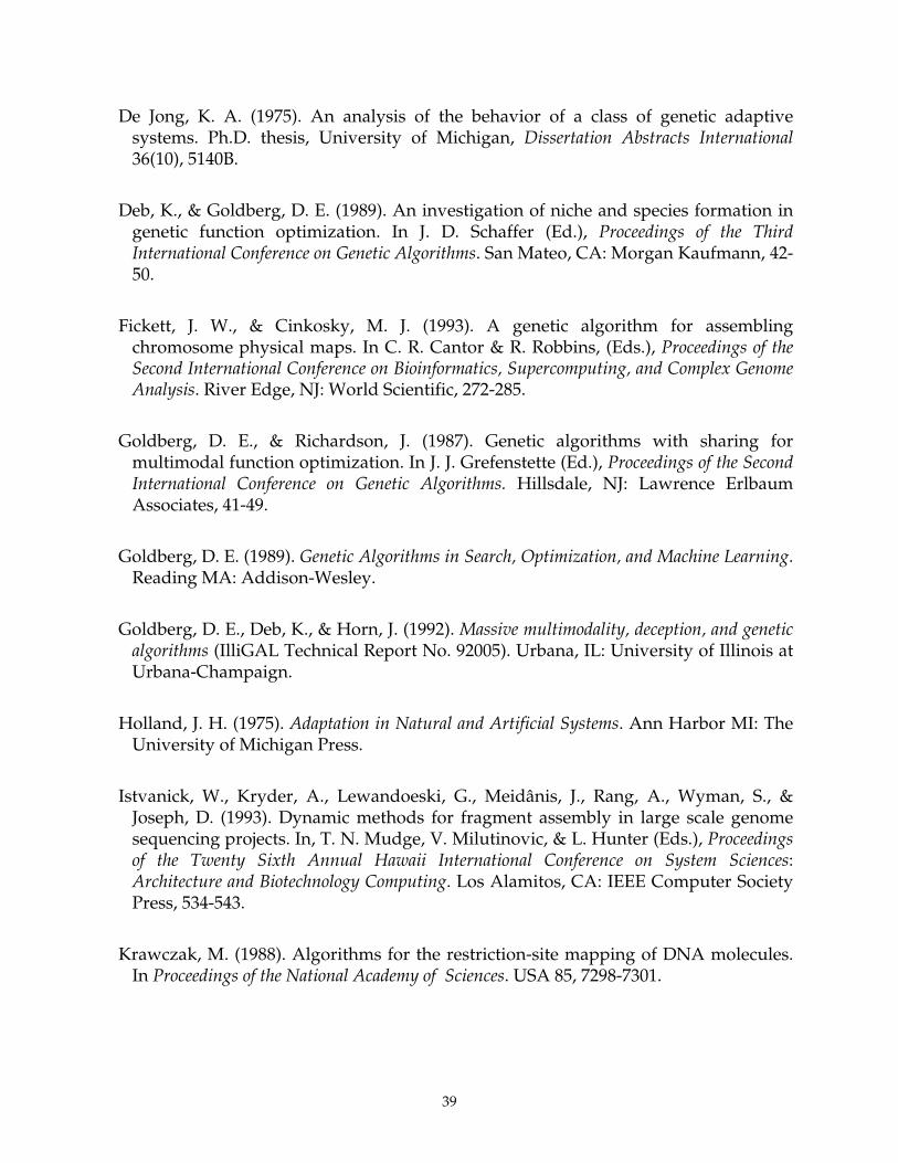
Function F3(x,y), called “Shekel’s foxholes” with twenty five optima, was used by De

Jong in his work on crowding. The inverted version of F3 is shown on Figure 3. The

peaks are located on the grid intersections formed by the values x = [32, 16, 0, -16, -32]

and y = [32, 16, 0, -16, -32]. All 25 peaks have the same base width. The height of peak i

is given by the expression 0.002 + 1/i, where the peaks are located at (32, 32), (16, 32), ...,

10

(-32, -32). Using a value of C = 2 a GA using crowding consistently found the global

optima. Crowding allows the GA to escape local optima by maintaining diversity in the

population during the early stages.

Figure 3: Test Function F3(x), Inverted Shekel's Foxholes.

We also considered other functions not exhibiting the symmetry present in the

above functions. Function F4(x,y), shown on the left in Figure 4, contains two global

optima with the same height and width but located far apart. Function F5(x,y), the

sample shown on the right in Figure 4, contains five optima with height, width, and

location chosen at random in every run. Both of these functions are defined by the

summation:

AiWi x Xi y Yii

p

1 2 21 + − + −=

∑(( ) ( ) ) ,

where p indicates the number of peaks in the function, (Xi, Yi) the coordinates of peak i,

Ai is the height of peak i, andWi determines how narrow or wide the base of peak i is.

Table 1 summarizes the parameters for functions F4 and F

5 shown in Figure 4.

11

Table 1: Parameters for functions F4 and F

5.

Function Peak Location Width HeightF4 (45k, 2k) 0.0004 100

(15k, 62k) 0.0004 100F5 ( 17.1, 34.4 ) 1.9 50.5

c1.coord[( 8.7, 4.1 ) 0.17 44.8( 20.3, 11.0 ) 3.6 87.1( 38.3, 47.9 ) 3.1 51.5( 57.9, 54.1 ) 3.7 55.5

Figure 4: Test functions F4 (scaled version on left) and F5 (right).

The MNC method was applied on these test functions and the simulations were

done on a 486/33MHz PC. The variables x and y were encoded using two 32 bit

chromosomes. The initial population was generated at random. Interval crossover was

used for mating. In interval crossover only one offspring is generated. For each pair of

parent chromosomes, x1 and x2, (assume without loss of generality that the cardinal

value of binary string x1 is less than the cardinal value of binary string x2), the

offspring’s chromosome is selected at random from the interval [x1-δ, x2+δ]. The value

for δ is usually small. This allows the offspring to move outside the boundaries

delineated by their parents. For this test δ was set at the decimal value 1,000. We

obtained better results using interval crossover over single-point crossover. This is due

in part to the disruptive effect on niche preservation caused by single-point crossover.

12

For example, consider the individuals 0100000000000 and 0011111111111. If these

individuals are part of the same peak, a single-point crossover may conceivably

generate the offspring pair 0000000000000 and 0111111111111 which may not be in the

same peak as the parents. On the other hand interval crossover will generate an

offspring close to the parents and more likely to belong to the same niche. After mating

bit mutation is applied to the offspring.

The crossover probability (pc) was set at 0.95. Normally one tends to choose a lower

value for the crossover probability in order to allow individuals to survive from one

generation to the other. In contrast, in the MNC, pc is usually chosen in the interval [0.9,

1.0] for three reasons. First, the individuals with highest fitness will survive multiple

generations. Second, low pc values tend to increase the number of duplicate

chromosomes in the population. Third, offspring are likely to replace individuals with

similar phenotypic features and thus alleviate the need to carry other individuals. The

mutation probability (pm) was set at 0.001. Mutation may allow an individual to escape

from a niche to other areas not explored by the algorithm. Furthermore, it is useful to

note, in passing, that duplicates encountered after mating (mating pair do not undergo

crossover and mutation) or during replacement (offspring same as individual in

population) are not inserted in the population.

The phenotypical similarity between two individuals was determined by the

Euclidean distance between them. Like Deb and Goldberg (1989) we also had better

performance when the similarity was based on the phenotype rather than the genotype.

The MNC method was executed for 100 generations in each run. Other parameters are

summarized in Table 2.

13

Table 2: Function Specific Parameters used in the MNC method.

F1 & F

2F

3F

4F

5

Population size (N): 100 500 100 200

Number of chromosomes: 1 2 2 2

Crowding selection size (Cs ): 15 75 5 15

Crowding factor (Cf ): 2 2 3 3

Crowding factor group size (s): 15 75 5 15

These parameters were chosen after a number of trial runs. Although the optimal

value of these parameters is unknown at this moment, a rule of thumb that worked fine

on these functions was the following. The population size was selected to be N ≥ 20p,

where p is the number of peaks. This value of N allowed small peaks to survive for

many generations and the need to use a large population is avoided.

For the crowding selection size, Cs, and the crowding size, s, the values where

chosen to be at least 2p. The idea is to get a group size that will likely contain an

individual from the same niche during selection or replacement. At the same time it

must be small enough to allow competition between different niches. A large group size

will restrict selection and replacement among members of the same niche only. For

these test function a value of 3p for Cs and s produced good results. The crowding

factor, Cf, was set at 2 or 3. Higher crowding factor values increased the chances of high-

fitness individuals to survive for more generations. On the other hand higher values

can cause niches from small peaks to dissapear from the population in less number of

generations.

These parameter values seem to balance competition between individuals in the

same niche and individuals from different niches. Consider for example a value of Cs =

1. This will reduce the selection step to basically random selection as is used in

14

deterministic crowding. Increasing the value of Cs will localize a mate closer to the

parent. For very large values, i.e. , Cs closer to N, the mate chosen will most likely be the

parent itself.

The same applies during replacement for the value of s. What is interesting is the

effect of the combined values of s and Cf during replacement. A value of s > 1 and Cf = 1

reduces the replacement step to crowding and fitness plays no role in the MNC method.

These settings will reduce the method to some form of random search since fitness is

not used during selection. Consider now s = 1 and Cf > 1 during replacement. In this

case similarity plays no role and only fitness is used during replacement. Higher peaks

will tend to take over the population with these settings. At a minimum both s and Cf

must be greater than 1 to allow multiple niches to survive. Increasing s will promote

more competition between members of the same niche. Increasing Cf will allow fitness

to play a bigger role during replacement. An analysis of the MNC method and the effect

of these parameters is ongoing and will be reported in another paper.

An interesting approach will be to allow the parameters Cs, s, and Cf to dynamically

change with the population. This will allow the algorithm to adapt itself to the

idiosyncracies of the search space. A related idea, based on implicit fitness sharing,

(Smith et al., 1993) effectively maintained diverse populations while modeling the

immune system.

3.1 Results on Multimodal Test Functions

For all test cases the MNC method was able to maintain stable subpopulations in

most of the peaks without converging prematurely to any one of them. Only very small

peaks in F3 and F5 did not have any significant number of individuals in the last

generation even though some were present during many earlier generations. All peaks

in functions F1, F2, and F4 were found. Even the local optima at x = 1 was found in F1 and

was kept until the last generation. Stable subpopulations were consistently maintained

15

in all peaks until the last generation. The distance between the peaks in F4 did not cause

any problem for the MNC method. Figure 5, shows for function F4, the average fitness

of the individuals (on the left) in each peak and the number of individuals (on the right)

in each peak. The results were averaged over 20 runs. An individual solution is

considered part of a peak if it is located in the region above 10% of the height of the

peak. The solid line represents individuals located in neither peak. As can be seen the

number of individuals stabilizes around the same time as the average fitness does. After

that the number of individuals in the peaks does not fluctuates greatly for the last 70+

generations.

0

10

20

30

40

50

60

70

80

90

100

0 10 20 30 40 50 60 70 80 90 100Generation Number

Ave

rag

e F

itn

ess

Peak 1

Peak 2

Others

0

10

20

30

40

5060

70

80

90

100

0 10 20 30 40 50 60 70 80 90 100Generation Number

Nu

mb

er o

f In

div

idu

als

Peak 1

Peak 2

Others

Figure 5: Average fitness (left) and number of individuals (right) for function F4.

In general, the number of individuals at the lower peaks decreased as the fitness of

the individuals in other peaks increased. During the initial generations all peaks had

about the same number of individuals since their average fitness was comparable. As

the average fitness increased in some peaks so did the number of individuals in those

peaks. In other words, the number of slots in the population occuppied by a peak

depends on its average fitness relative to that of other peaks. Of course there are other

factors affecting the peak count and that needs to be studied further. As the average

fitness approaches a peak’s optimum, the number of individuals in that peak stabilizes.

This can be observed in Figure 6 for peak 2 located near (0,0) and all other peaks in

function F5. The plot on the left has the average fitness of each peak for every

16

generation. The plot on the right has the number of individuals in each peak for every

generation. During the initial ten generations the wider peak (peak 2) had more

individuals in the population. As the fitness of the individuals in the other peaks

improved the number of individuals increased. After about 20 generations the number

individuals in the other peaks was greater than those in the wider peak. There are of

course other factors that contribute to this pattern and that needs to be investigated

further. It shows the ability of the MNC method to avoid premature convergence.

0

10

20

30

40

50

60

70

80

90

0 10 20 30 40 50 60 70 80 90 100

Generation Number

Ave

rag

e F

itn

ess

Peak 1 Peak 2Peak 3 Peak 4Peak 5 Other

0

10

20

30

40

50

60

70

0 10 20 30 40 50 60 70 80 90 100

Generation Number

Nu

mb

er o

f In

div

idu

als

Peak 1 Peak 2

Peak 3 Peak 4

Peak 5 Others

Figure 6: Average fitness (left) and number of individuals (right) for function F5.

We also observed that the number of individuals in a peak is related to more than

just its average fitness. In function F3 where the optima are located on a 5x5 grid, peaks

along the same x and y axis as the global optima had more individuals than other peaks

with higher average fitness. Some of the extra individuals can be attributed to mutation

since a bit change in one of the chromosomes will cause an individual to move along the

x or y axis. We ran the same test with mutation set at 0.0 and no major changes were

observed. More analysis is needed to determine other factors affecting the number of

individuals in a peak.

The properties exhibited by the MNC method are encouraging. The population

converges to multiple optima and stable subpopulations evolve in different niches.

Three main factors appear to contribute to the success of the algorithm. First, using

17

crowding selection and worst among most similar replacement allowed niches to form

naturally and compete for population slots among them. Second, the mating operator

used preserved parents’ phenotype in the offspring and therefore allowed individuals

from a niche to generate offspring in the same niche. Third, phenotypic similarity

allowed individuals to form niches in the solution space. Although a more rigorous

analysis is necessary before the merits of this method can be substantiated, this method

is applied nevertheless to solve the problem of DNA restriction-fragment assembly, a

problem widely believed to be NP-hard.

4. Background on the DNA Restriction-Fragment Assembly Problem

The purpose of this section is to provide a simplified summary of the biological

background necessary to understand some of the central issues in the DNA restriction-

fragment assembly problem as it arises in the Human Genome Project.

The genetic material contained in all the chromosomes of a cell is collectively called

the genome. Chromosomes are essentially DNA molecules, the ladder shaped, double-

helical structures. For the purpose of this paper, suffice it to say that the most important

parts of this double-helix are the "steps" of the ladder. These steps, called base-pairs,

denoted here by the letters A, C, G, T, can theoretically form sixteen pairs. However,

only AT, TA, CG and GC pairings are allowed. That is, if the left half of the base-pair is

known, the right half is uniquely determined and vice versa. It is estimated that the

human genome, contained in all the 23 pairs of chromosomes, is comprised of about

three billion base-pairs. A hypothetical sequence of these may look like

AATCTTCGGGCCT.... occupying three billion positions. Specific sub sequences of this

are called genes.

The monumental task of the Human Genome Project is to (a) associate with each

gene all the properties controlled by that gene, (b) associate each gene with one of the 23

chromosomes in the body, (c) identify the exact positioning of a gene on a chromosome

18

- known as the mapping problem or the genetic-linkage problem, and (d) decipher the

exact sequence of base pairs that constitute a given gene - known as the sequencing

problem. Although each human is uniquely characterized by his/her genome,

apparently one individual differs from another in only a small percentage (about 0.2%)

of this material. For that matter, the human genome differs from the simian genome by

only a few percentage points. Thus the Human Genome Project is only analyzing a sort

of composite genome: 23 chromosome pairs donated by a few European and U. S.

scientists. Thus, the focus is on understanding the common structure that runs through

the human species, although the actual DNA used in the experiments may come from a

specific individual.

Issues related to molecular biology, instrumentation and computations do play a

critical role in this effort. It is impractical even to attempt to summarize the scope of this

project here. A description of the technique used, at the Human Genome Center of the

Lawrence Livermore National Laboratory (LLNL), for example, can be found in

Genomics, 4, pp 129-136 (Carrano et al. 1989). To view on-line information about, say the

LLNL genome program, it is only necessary to point the WWW client at: http://www-

bio.llnl.gov/bbrp/genome.html. This Center is mapping human chromosome 19 which

is estimated to be approximately 60 million base-pairs long, a relatively small-sized

chromosome.

Current technology is forcing us to limit the sequencing task to small fragments of

DNA that are composed of approximately 0.5K base-pairs (Istvanick et al. 1993). In

order to divide the DNA into fragments up to this resolution level, techniques using

restriction enzymes are used. The restriction enzymes act on the DNA at specific

locations which are randomly distributed along the length of the chromosome.

Depending on the number of different restriction enzymes used in obtaining the

fragments, the data are called single-digest (one enzyme), double-digest (two enzymes),

19

or n-digest (n enzymes) data. Most mappings are done using single- and double-digest

data. Scientists use different restriction enzymes to obtain DNA fragments of the

appropriate size.

In practice, scientists try to map one chromosome at a time. Many techniques

generally require: (a) purifying chromosomal DNA, (b) cutting the DNA into pieces

called contigs using restriction enzymes, (c) inserting contigs into DNA cloning vectors,

(d) inserting cloning vectors into bacterial host cells for multiplication, (e) cutting clones

into fragments, (f) analyzing the fragments, and (g) reconstructing the original order of

the base-pairs on the chromosome.

4.1 Restriction Fragment Data for Chromosome 19

As the data used in this study are obtained from the Human Genome Center of

LLNL, it is useful to summarize the techniques used at LLNL to gather these data.

Chromosomes are sorted via a laser flow sorter; restriction enzymes are used to

shatter the sorted material into fragments. These fragments are inserted into a host

vector which can then be grown in large quantities. Due to the properties of the cloning

vector used at LLNL, our so-called cosmid clones average 40Kbp (forty thousand base

pairs) of DNA each. It is important to note that in each such cloning step, all original

order is lost.

The LLNL biologists cloned and selected 15,000 such cosmid clones for human

chromosome 19. A "cosmid fingerprint" was obtained for each clone by subjecting them

to a double-digest labeled with a fluorescent dye and measuring them on a modified

DNA sequencing gel apparatus. These crude fingerprints were compared between all

pairs (taking 2 days on a network of 40 workstations in parallel) and a set of 800

unordered islands or "contigs" were formed by an automated algorithm which also

determined a near-minimal spanning path for each island. (Note that 15,000 40Kbp

20

clones provides a nominal 10X depth of coverage for chromosome 19.) However, this

set of islands remains unordered by this technique.

A wide range of other techniques, not covered here, is used to merge, order, and

provide the distance between the contigs. This paper will focus on one technique used

to verify the accuracy of the contigs built via pair-wise overlap data, called EcoRI

restriction fragment mapping after the name of the restriction enzyme used. A subset of

the clones in a contig are chosen (i.e., the spanning path members plus other clones to

attempt to get at least a 2X coverage across the contig) and digested, with fragment

lengths in the range of about 0.5-20Kbp being generated, depending on the distribution

of EcoRI sites within each cosmid. These maps are of great utility in locating and

sequencing genes; since individual EcoRI fragments can be physically cut from gels and

prepared for sequencing, the cost of sequencing a gene can often be reduced by an

order of magnitude (assuming a gene can be localized to a ~4Kbp fragment, instead of

having to sequence an entire 40Kbp clone).

The order of the fragments within each clone is of course unknown. At LLNL, the

"EcoRI maps" are constructed rapidly by hand, since the existence of a reliable near-

minimal spanning paths provides a tremendous hint towards obtaining a proper clone

ordering. This in effect reduces a 2-D optimzation problem to a 1-D one. Once clone

order is known, fragment ordering within clones is a much simpler problem (note that

fragment sizes can be measured to about 5%, and that fragments of the same size can

occur in multiple unrelated positions within a single map.)

The process of initially assembling the contigs and thereby deriving the minimal

spanning paths is itself quite slow and labor-intensive in terms of laboratory bench

work. LLNL researchers were interested in seeing how well a fully-automated system

could do in assembling EcoRI maps if a priori contig information were not available.

This is the problem discussed here: given a number of clones, in unknown order, each

21

with a set of restriction fragments, also in unknown order, construct a maximum-

likelihood map of that region, subject to the constraints that, in general, the cosmids

should be contiguous in the resulting maps, and apart from end fragments, all

fragments should overlap others in their vertical "stack" within about 5% of their

lengths. If these maps could be build accurately over large regions (i.e., at least 200-

500Kbp), a potential exists for reducing the overall cost of obtaining a high-resolution

physical map.

Chromosome is divided into several islands (contigs)

Clone restriction fragments (.5 - 15 kbp)

Contig map ofoverlappingcosmid clones( ~150 kbp)

Contig

Figure 7: Physical map for island using fragments from a set of overlapping clones.

Toward the goal stated above, in this paper, we propose to establish the relative

position of each cosmid clone on a contig by establishing the possible locations of the

fragments in each cosmid clone in such a manner that the fragment overlap among the

clones is maximized while a suitably defined total error between the overlapped

fragments is minimized. There are other constraints such as the total length of the

assembly be equal to the contig's original size. The problem is one of assembling cosmid

clone sequences as shown in Figure 7. The problem is complicated further by the

22

uncertainty in the data, the possibility of data loss (fragments of the same size are hard

to distinguish during fingerprinting), and the known fact that data related to corner

fragments (i.e., fragments near the fragment boundaries) is almost always unreliable.

Problems of this type are known to be hard (Opatrny, 1979). For example, the case with

10 cosmid clones, there are 10! / 2 possible clone sequences.

4.2 Related Work and Scope of Present Work

The DNA restriction fragment assembly, the subject matter of this paper resembles,

and is somewhat related to, the restriction-site mapping, which deals with the equivalent

problem of determining the absolute location of a fragment within a cosmid clone. Here

also one uses digestion data from restriction enzymes but the focus is on finding the

absolute location of a fragment on a clone. Stefik (1978) used a branch and bound

technique with rules to exhaustively eliminate wrong answers from the digest fragment

data. This approach is sensitive to error in the data and is computationally intensive.

Pearson (1982) exhaustively generated permutations of the single-digest data to

compute the error between the generated double-digest and the actual (experimental)

double-digest data. This approach is faster but it is limited to small number of

restriction sites also. Krawczak (1988) developed a divide and conquer technique that

groups the fragments into compatible clusters and then determine the order of the

fragments within each cluster. This approach can process a greater number of

restriction sites. Platt and Dix (1993) used Genetic Algorithms (GAs) for restriction-site

mapping using double digest data. In their work they did not consider operators suited

for multi-modal search spaces and mating which preserve adjacency information.

Other techniques are available to sequence larger DNA regions. Branscomb et al.

(1990) developed a greedy algorithm to order the most probable clone sequence using

overlap probabilities between the clones. The algorithm works well when a large

amount of overlap between the clones exists and the fragment data has small errors.

23

This approach is prone to getting stuck in local minima and does not use all the

available data gathered at great expense. Techniques using larger clones are also being

tried to order, orient, and connect the islands in the original DNA (Olson et al. 1986;

Waterman and Griggs 1986; Stallings et al. 1990; Fickett and Cinkosky 1993).

Cuticchia et al. (1992) constructed maps using simulated annealing techniques. In

their work clones are ordered according to a measure of similarity between them given

by the presence or absence of specific sequences. A signature is assigned to each clone

and the algorithm uses it to minimize the error between the actual length of the contig

and the given length by the hypothetical clone ordering. Matching signatures are use to

order the clones. In their work they only considered the relationship between

consecutive clones.

Recently, Parsons et al. (1993, 1995) applied the edge recombination crossover (Whitley

et al. 1989) in conjunction with several specialized operators and solved a 10 Kbp

sequencing problem consisting of 177 fragments with no manual intervention.

Previously, we too had experimented, although not reported, with a variety of

permutation-based crossover operators, such as those one finds in Traveling Sales

Person type problems. In that context we also found and reported that the edge

recombination operator outperformed the permutation-based operators by a wide

margin (Cedeño and Vemuri, 1993). In this paper, we now describe a genetic algorithm

that uses single-digest restriction data on a set of overlapping clones to find multiple

solutions for the clone sequences. We use genetic operators suited for multi-modal

function optimization (Cedeño and Vemuri, 1992) to determine solutions. A mating

operator based on genetic edge recombination was used to preserve adjacency

information and improve convergence toward multiple solutions at the same time.

Results are given for two data sets of overlapping clones from human chromosome 19.

24

Before delving into the details of the application of MNC algorithm to the DNA

problem, it is useful to pause and justify the need for multi-modal optimization to solve

this problem. We are aware of the fact that molecular biologists, unlike engineers,

cannot use “sub-optimal” solutions. As any geneticist knows, one missing or misplaced

base-pair could lead to the synthesis of an entirely different protein. Ideally, what a

molecular biologist wants is the exact sequence, which should correspond in our

mathematical formulation to the global optimum. But the search for this global

optimum is intimately tied up with the selection of the optimization criterion, say the

fitness function in GAs or the optimization criterion such as an energy function in

classical optimization. As long as this criterion is fabricated by our methods, we will

never be able to zero in on the “correct” solution using mathematical methods. The best

we can do is to ease the burden on the biologist by showing her (him) possible avenues

for further experimental investigation. We believe that this is the place the sub

optimization plays a role and that is the reason we were searching for the k-best sub

optima.

5. Problem Representation

It is worth repeating the cautionary word about the terminology used here.

Hereafter, the word DNA is used synonymously with the word chromosome(s) found

in a cell, whereas the word chromosome will be used to describe the computational data

structure used in genetic algorithms. This interesting situation arose because genetic

algorithms are computational processes that imitate natural processes of selection and

survival. Coincidentally, we are applying this metaphorical computational paradigm to

solve a problem in genetics! So it is important to distinguish meanings of terms used in

the problem domain from those used in the paradigm domain.

In this section some problem-dependent genetic operators are defined. First, the

encoding of the chromosomes to describe clone sequences is examined. Second, the use

25

of fragment sizes to define the fitness function is described. Third, the modified edge

recombination mating operator is described. And last, the function that measures

similarity between two clone sequences is described.

ALLELE CLONENUMBER ID FRAGMENT SIZES (in thousands of base-pairs) C0 5154 16.55, 4.4, 1.68, 1.07, 4.81, 8.5 C1 7442 0.79, 0.79, 2.6, 4.35, 8.24, 2.7, 6.9, 5.16 C2 21230 0.96, 1.68, 1.08, 4.77, 8.47, 1.44, 2.37, 6.29, 0.62 C3 8131 0.92, 3.73, 19.8, 4.43, 1.69, 1.25, 4.68, 5.63 C4 18993 0.96, 6.31, 5.48, 8.61, 7.29, 0.81, 0.81, 2.6, 4.36, 1.92 C5 5435 2.89, 8.24, 2.7, 6.9, 5.14, 5.14, 2.89, 1.54 C6 7255 1.04, 8.21, 2.69, 6.89, 5.12, 5.12, 2.88, 1.94, 2.42, 1.37, 3.33 C7 12282 4.52, 5.13, 5.13, 2.87, 1.94, 2.42, 1.39, 3.35, 5.41 C8 27714 6.69, 5.07, 5.41, 2.88, 1.92, 2.32, 1.4, 3.35, 5.46, 17.65, 1.0, 10.49, 0.58, 1.74 C9 10406 2.03, 1.43, 2.34, 6.28, 5.46, 8.58, 7.27

Figure 8: Cosmid clones with fragment data.

Before going into the details about the operators, it is important to show how the

data for the problem is presented to the GA. Figure 8 shows fragment sizes obtained

from fingerprinting for a set of overlapping cosmid clones. For example, cosmid clone

with the ID number 5154 which is also labelled as Allele Number C0, is known to be

comprised of six fragments, containing 16550, 4400, 1680, 1070, 4810 and 8500 base-

pairs, in that order. Also, cosmid clone with the ID number 8131 which is also labelled

as Allele Number C3, is known to be comprised of eight fragments, containing 920,

3730, 19800, 4430, 1690, 1250, 4680 and 5630 base-pairs, in that order. By comparing

these fragment sequences one can surmise that the third and fourth fragments of Allele

C0 are probably the same as the fifth and sixth fragments of Allele C3 mainly because

the fragment lengths are so nearly equal to each other. If this is true then Alleles C3 can

be "aligned" below Allele C0 in such a manner that the fifth and sixth fragments of

Allele C3 fall right below the third and fourth fragments of Allele C0 as shown in Figure

9. The matching of the fragment lengths is not perfect. Indeed, the mismatch at other

positions is large. The goal of this problem is to maximize this type of matching while

minimizing the number and degree of mismatches while keeping the total length of the

26

assembly within reasonable limits. The data for this problem consist of the n cosmid

clones with their fragment lengths and the tolerance measure e which is used to

determine if two fragments are of the same size. That is, two fragments F1 and F2 are

considered to be of the same size if |F1 - F2| < e.

Clone Fragments

C3 8131 0.92 3.73 19.8 4.43 1.69 1.25 4.68 5.63C0 5154 16.55 4.4 1.68 1.07 4.81 8.5C2 21230 0.96 1.68 1.08 4.77 8.47 1.44 2.37 6.29 0.62

Figure 9. An example of fragment assembly.

5.1 Chromosome Encoding

The encoding for this problem is simple. Each allele in the chromosome has a label

between 0 and n - 1 corresponding to one of the cosmid clones. No two alleles have the

same label, and mating and mutation will preserve this constraint. In Figure 8, for

example, an allele with the label C0 corresponds to the clone with ID 5154 and an allele

with the label C9 corresponds to clone ID 10406. The clone sequence (5154, 21230, 10406,

7255, 12282, 27714, 8131, 18993, 7442, 5435), for example, is represented by the

chromosome (0 2 9 6 7 8 3 4 1 5). The initial population is generated by picking, at

random, values between 0 and n - 1 without replacement.

Number of matches between clones Total error in the matches CLONE C0 C1 C2 C3 C4 C5 C6 C7 C8 C9 C0 C1 C2 C3 C4 C5 C6 C7 C8 C9 C0 6 1 4 2 1 0 1 0 2 1 0 5 8 4 4 0 3 0 13 8 C1 1 8 0 1 4 4 4 1 1 0 5 0 0 8 5 2 9 3 9 0 C2 4 0 9 3 2 1 3 2 5 3 8 0 0 14 2 10 16 10 23 5 C3 2 1 3 8 2 0 0 1 2 0 4 8 14 0 11 0 0 9 13 0 C4 1 4 2 2 10 1 3 2 3 4 4 5 2 11 0 10 19 9 6 10 C5 0 4 1 0 1 8 6 3 2 0 0 2 10 0 10 0 10 4 8 0 C6 1 4 3 0 3 6 11 7 7 3 3 9 16 0 19 10 0 7 26 23 C7 0 1 2 1 2 3 7 9 7 4 0 3 10 9 9 4 7 0 20 26 C8 2 1 5 2 3 2 7 7 14 3 13 9 23 13 6 8 26 20 0 5 C9 1 0 3 0 4 0 3 4 3 7 8 0 5 0 10 0 23 26 5 0

27

Figure 10: The M matrix on the left whose entries are the number of fragmentmatches and the E matrix on the right whose entries are the total errors between anytwo clones with ε = 10.

5.2 Fitness Function

To calculate the fitness of an individual, the number of fragment matches between

all consecutive clones and the error between the fragments is considered. The fragment

sizes are represented using integer numbers (by multiplying the number given in

Figure 8 by 100), to accelerate computation of the fitness function. Prior to the execution

of the GA, two matrices are calculated. One matrix, the match matrix M shown on the

left side of Figure 10, contains the number of fragments that match between two clones

Ci and Cj, within an error tolerance ε . The other matrix, the error matrix E shown on

the right side of Figure 10, contains the total error between the clones being matched.

The error between two clones is given by the sum of the errors between all fragments

that matched. For example, between clone No. 8131 (C3) and clone No. 5154 (C0) there

are two pairs of fragments that match within the specified tolerance of ε = 10. The

lengths of these fragments are 169 and 168 for one pair and 443 and 440 for the second

pair. Thus a 2 appears in (row 2, column 4) of the Match Matrix M. The total error

between both pairs of fragments is (169-168) + (443-440) = 4, which is shown in (row 1,

col. 4) of the Error Matrix, E.

Our goal is to arrange the cosmid clones as shown in Figure 7 so that the lengths of

the overlapping fragments match with each other as closely as possible. The necessary

matching information is already gathered in the matrix M and the degree of

accumulated mismatch per clone is gathered in the matrix E. However, we believe that

this information alone is not sufficient to establish which two clones are "adjacent" to

each other in the arrangement shown in Figure 7. For example, consider how clone C0

(i.e., allele No. 5154) matches with other clones. Inspection of the match matrix M

indicates that the degree of match between clone C0 and clone C2 (or, equivalently,

28

allele No. 21230), is 4 matches. Also, fragments in clone C0 match with fragments in

clone C3 as well as C8, each with 2 matches. By interpreting this to mean that C2 should

be placed nearer to C0 than C3 or C8, we are ignoring information contained in the C0-

C3 matches and C0-C8 matches. One more example suffices to make the point. Clone C3

should be placed closer to C2 because they match with each other the maximum

number of times, namely 3, although C3 matches with three other clones, each with

only 2 matches. This phenomena makes us to think that using only the number of

matches between clones is not sufficient to establish the partial order between clones

when they possess the same match count. We believe that part of this problem is due to

false matches, between fragments of similar sizes, that may occur by chance. We tried to

overcome this problem by incorporating the total error in the matches, shown in matrix

E, in order to enable our GA to discriminate further between clones. Using the same

example, notice that clone C3 has less total error when matched with C0 than clone C8

and therefore indicates that C0 is adjacent to C3. The following equation for fitness

captures the essence of the method described so far.

fitnessM a a

Count a

E a a

M a ai i j

i j

i i j

i i jjj

i

n= −

⋅

+

+

+

+= −≠

=

−∑∑

[ , ]

[ ]

[ , ]

[ , ]1

10

1

0

1

ε

Here ai refers to the cosmid clone placed in the ith position of the chromosome, ai+j

refers to the clone to the right or left (if any) of the ith position. The first term,

M[ai,ai+j]/Count[ai+j], give us a normalized count for the degree of match. The term

E[ai,ai+j]/M[ai,ai+j]⋅ε refers to the normalized error per fragment. When this normalized

error reaches unity, it means that the total error is so large that any apparent matches

are worthless. With this interpretation, the second term of the equation essentially tells

us the degree of confidence we can place on the normalized matches we are counting in

29

the first term. In the above equation, n refers to the number of alleles in the

chromosome which is equal to the number of clones.

By defining the fitness function as above, we are assigning a higher fitness to those

clone pairs that match a higher percentage of their regions. For example, Allele 0 with 6

fragments has two matches each with Alleles 3 and 8, each having 8 and 14 fragments

respectively. Since 2/8 represents a higher percentage than 2/14, we designed a fitness

function that prefers a configuration that places Allele 3 closer to Allele 0 than Allele 8.

This is achieved by dividing the number of matches by the number of fragments in the

clone.

Before settling on the fitness function described above, others were considered. For

example, fitness functions that just counted the number of matches between clones with

no regard to normalization failed to produce the correct answer. A fitness function that

just counted the number of matches and then subtracted the total error in those matches

also failed to give satifactory results. It is possible that other fitness functions may give

results that are even better than what are reported here. In the future, we plan to

include the number of matches as well as errors among groups of three clones or more

as components of the fitness function and study its effect on performance.

5.3 Mating and Mutation Operators

The mating operator used in this method is based on a slight modification to the

genetic edge recombination operator that was applied successfully to solve the TSP

(Traveling Sales Person) problem. As in the TSP problem, the important information

here is the adjacency of the alleles, although the order the alleles appear in the

chromosome can be derived from the adjacency information. The idea is to recombine

the links (pairs of clones) between two parents such that common links are inherited by

the offspring. This operator is implemented in two steps as shown in Figure 11. First,

those links (or traits) that are common to both the parents are identified and passed on

30

to the offspring and the links occupy the same absolute positions in the offspring

chromosome. In the example shown in Figure 11, the relevant link-pairs are 7-8, 8-1,

and 5-0 in the first parent and 1-8, 8-7 and 5-0 in the second parent. Notice that these

links are passed on to the two offspring undisturbed. Second, those alleles that are not

passed to the offspring (indicated by dashes, in Figure 11) are randomly assigned to the

available positions while observing the constraint that no link label is repeated.

Parent 1 Common links (traits) Offspring 1 (6 7 8 1 2 3 9 4 5 0) (- 7 8 1 - - - - 5 0) (3 7 8 1 4 6 2 9 5 0)

Parent 2 Common links (traits) Offspring 2 (1 8 7 9 5 0 2 6 3 4) (1 8 7 - 5 0 - - - -) (1 8 7 3 5 0 6 2 4 9)

Figure 11: Modified genetic edge recombination for clone sequencing.

The differences between this operator and the original edge recombination operator

are in the number of offspring generated and in the assignment of alleles not transferred

from the parent. We generated two offspring instead of one because the location of the

links in the clone sequence is important to our problem. In TSP the chromosome is

circular, thus the location did not matter. We allow both parents to pass the location of

the links to their offspring. To assign the other alleles we select them at random from

those clones not passed by their parents. In the original operator the links are assigned

from those present in any of the two parents. Alleles with fewer links are assigned first

to prevent from running out of links for a given allele.

In the mating operator used here there is excessive exploration of the search space

primarily due to the random filling of the unassigned slots, in the second step, while

creating the offspring chromosomes. Part of this exploration difficulty is alleviated by

the fact that mates are selected using crowding selection and therefore they have

common features between them. Exploration is therefore localize to a smaller region

within the entire search space. On the other hand, by allowing unassigned clones to be

31

chosen at random, we are allowing links to re-appear that might not have done so using

mutation alone. Other crossover operators based on clone positions alone did not

perform as well in this problem, we only give the results for the modified edge

recombinator operator.

Mutation is applied on an individual basis. After an offspring is generated it is

mutated if the outcome from the flip of a biased coin is true. When this happens, a link

from the offspring is selected at random and all alleles from that link to the last position

of the chromosome are reversed. For example, the offspring ( 1 8 7 3 5 0 6 2 4 9) after

mutation can result in ( 1 8 7 9 4 2 6 0 5 3) if the link between allele 7 and 3 is selected to

mutate. This mutation operator is known as inversion (Holland 1975).

The mating and mutation operators are compatible with each other in the sense that

they both operate on links. The building blocks of this problem are based on the links

between clones in the sequence. The GA operates on these links so that the most useful

ones are passed from generation to generation.

5.4 Similarity Function

The similarity function is very simple also. It counts the number of dissimilar links

between two individuals. Using the parents from Figure 11 once again as an example,

notice that there are six dissimilar links, corresponding to the five alleles not assigned to

the offspring. For concreteness, these six dissimilar links in Parent 1 chromosome are 6-

7, 1-2, 2-3, 3-9, 9-4 and 4-5 and for Parent 2 are 7-9, 9-5, 0-2, 2-6, 6-3 and 3-4. This metric

measures the proximity between two clone sequences by counting the different links

they have and not the position of the alleles. For example, the sequences (0 1 2 3 4 5 6 7 8

9) and (9 8 7 6 5 4 3 2 1 0) have a distance of zero since all the links are the same. This

metric captures the essential aspect of the problem since both solutions are equivalent in

our problem.

32

6. Results and Discussion

The results presented in this section were obtained on a SGI IRIS 4D computer

under IRIX O.S. running the GA application written in C. The parameters for the GA

are the following:

Population size: 100

Mutation probability: 0.06

Crossover probability: 1.00

Crowding selection group size (Cs) 20

Crowding factor group size (s): 10

Crowding factor (Cf): 5

Maximum number of generations to execute: 100

Tolerance ε 10

These parameters were selected after various trials. In each trial, different values for

each of the six parameters were tried, varying one at a time while holding the others

constant. A population size of 100 was found satisfactory. Other sizes (50, 150, 200, 250,

and 300) were tried. Higher sizes did not provide new information about the problem,

although they produced, on average, the solution in less number of generations. Lower

sizes in some cases did not converge to the best solutions seen before in the allowed

number of generations. The population size of 100 is a compromise between speed of

convergence and execution time.

Mutation was set at 0.06, therefore an average of 6 individuals were mutated every

generation. This low value of mutation works well in this problem. It seems to allow

individuals to escape local optima without causing any major disruption on the

elements of a niche. In the MNC method diversity is maintained implicitly when the

population converges to different optima, reducing the need for higher mutation

values. On the other hand the mating probability was set to a high value of 1.0. As

described before the MNC method is basically a steady state GA and highly fit

33

individuals have a high chance of surviving for many generations. Also, crowding

selection exploits the similarity between individuals in the population by allowing

localize solutions to pass common traits between them.

The group size for crowding selection was set at 20. This high value emphasizes the

importance of similarity between parent and mate for this problem. Then the mating

operator will likely generate an offspring within the same region as their parents. The

size for the crowding factor groups was set at 10. This allowed competition between

multiple optima to occur while maintaining multiple solutions. Good results were

obtained with other Cs and s values (5, 10, 15, 20) also. The crowding factor was set at 5.

This value allowed the MNC method to eliminate low fitness individuals from the

niches more rapidly. These parameter values allowed a diverse population to co-exist

during the number of generations allowed and did not restrict competition between

individuals from different niches. The tolerance value ε was set to 10 to minimize false

matches due to chance. Higher values of ε increased the false matches more than true

matches and therefore more possible clone sequences were found.

The MNC method took an average of 50 seconds for each run. Some of the best

sequences obtained for two different data sets of overlapping clones are shown in

Figure 12. These results were obtained from 10 different runs. The figure shows the

actual sequence for the data sets and the clone sequences (with their fitness) obtained by

the algorithm.

Data for set 1 is shown in Figure 8 and data for set 2 is shown in the Appendix.

There was nothing really special about these data sets except that they were in regions

containing various gene(s) of interest to some of our collaborators. They had already

mapped them manually, so we could judge the answers our GA technique provided.

Finally, and perhaps most importantly, the data sets were large enough not to be toy

problems. One of the data sets contained two vertical "columns" in the final map that

34

had fragments of the same size. The existence of independent columns of the same size

is, of course, one of the things that makes this problem so tough, and interesting. Many

of the runs using data set 2 generated multiple solutions with relatively close fitness

values.

Data Set 1 actual sequence and its fitness:

(8131 5154 21230 10406 18993 7442 5435 7255 12282 27714) 764

The 3 Best sequences found by the GA and their corresponding fitnesses:

(8131 5154 21230 10406 18993 7442 5435 7255 12282 27714) 764 (8131 5154 21230 27714 12282 7255 5435 7442 18993 10406) 749 (8131 5154 21230 10406 27714 12282 7255 5435 7442 18993) 744

Data Set 2 actual sequence and its fitness:

(12595 6722 26999 29626 29064 18301 19811 29035 17755 28828 20235) 750

The 12 Best sequences found by the GA and their corresponding fitnesses:

(12595 26999 6722 29626 29064 18301 28828 20235 17755 29035 19811 ) 757 (20235 28828 17755 29035 19811 18301 29064 29626 6722 26999 12595 ) 757 (12595 26999 6722 29626 29064 18301 20235 28828 17755 29035 19811 ) 756 (28828 20235 17755 29035 19811 18301 29064 29626 6722 26999 12595 ) 755 (12595 26999 6722 29626 29064 18301 28828 20235 17755 19811 29035 ) 754 (12595 26999 6722 29626 29064 18301 20235 28828 17755 19811 29035 ) 753 (12595 6722 26999 29626 29064 18301 19811 29035 17755 28828 20235 ) 750 (20235 28828 17755 29035 19811 18301 29064 29626 12595 6722 26999 ) 750 (19811 29035 17755 20235 28828 18301 29064 29626 12595 6722 26999 ) 750 (19811 29035 17755 20235 28828 18301 29626 29064 26999 6722 12595 ) 750 (19811 29035 17755 28828 20235 18301 29064 29626 26999 6722 12595 ) 749 (19811 29035 17755 28828 20235 18301 29064 29626 12595 6722 26999 ) 749

Figure 12: Clone sequences obtained by GA and actual sequence.

For data set 1 the MNC method was able to find the actual clone sequence. The best

sequence as described by the fitness function did indeed match the solution. The best

sequence was found in all the runs. From the other sequences found, the fitness values

of the next best is 15 less than the actual sequence. Similar gaps exist between all the

sequences shown in Figure 12 for data set 1. From the solutions we can see that the

other sequences are a single mutation from the actual sequence.

35

Data set 2, shown in the Appendix, presented a more challenging problem for the

MNC method. In this case the best sequence found only had clones 6722 (C7) and 26999

(C2) transposed from the actual sequence. The fitness for the actual sequence is 750,

which is the sixth best score when compared with all solutions found. The actual

sequence was obtained in 8 of the 10 the runs. As shown in Figure 12, different solutions

with equal fitness values were found and maintained in the runs. Two different

solutions with a distance of 2 (two different links) were found with fitness equal to 757.

Four others were found with fitness equal to 750 (including the actual sequence).

Another observation is that there is a difference of 8 or less in the fitness between all the

sequences found. Some of the sequences are mutations of others, but there is more

diversity when compared with the solutions for data set 1. The biologists later

confirmed via independent techniques (i.e., hybridization probing) that the clones in

data set 2 were indeed from two distinct regions in the DNA. That is, the sequence

(6722 26999 12595 29626 29064 18301) and (19811 29035 17755 28828 20235) belong to

separate maps in the DNA. The best solutions found by the MNC method kept both

sequences apart.

0

100

200

300

400

500

600

0 10 20 30 40 50 60 70 80 90 100

Generation

Avg

Fit

nes

s

SGA

SSGA

MNC

300

400

500

600

700

800

0 10 20 30 40 50 60 70 80 90 100

Generation

Bes

t F

itn

ess

SGA

SSGA

MNC

Figure 13: Population average fitness (left) and best fitness (right) for different methods.

To see how the MNC method compares with more traditional GAs we applied the

same problem (i.e., using data set 2) to the SGA and SSGA with crowding. For both the

36

SGA and SSGA the crossover probability was set at 0.6. The crowding factor was set to

10 for the SSGA. All other parameters are the same as in the MNC method. We

observed poor results by the SGA using these parameters alone. To improve the

performance of the SGA the 10 best individuals in the population (known as generation

gap (De Jong 1975)) were transferred from the current generation to the next. Figure 13

shows the population’s average fitness (on the left) and the fitness of the best solution

(on the right) for the MNC, SGA, and SSGA methods averaged over 10 runs.

The MNC method outperformed both the SGA and the SSGA. The population

converged faster and at the same time kept multiple solutions throughout the run. Use

of a generation gap allowed the SGA to retain the good individuals found in previous

runs, but did not improve convergence towards multiple solutions. The SSGA did not

find the best sequence in any of the runs. The SGA found one of the two best sequences

in 2 of the runs. As mentioned before the MNC found the two best sequences and others

in 8 of the runs. The ability of the MNC method to exploit similarity and increased

competition among localized solutions proved to be successful in this problem.

7. Comments and Conclusions

Two points deserve further discussion. First, data containing clones with fewer than

five fragments were normally sequenced erroneously by the GA. This is due to the lack

of opportunity for sufficient fragment matches. Also data pertaining to corner

fragments (i. e., fragments lying near the cosmid clone boundaries) is generally more

prone to errors. Consequently corner segments will not match well with a high

probability with their counterparts in the preceding and succeeding clones. For clones

with less than five fragments, this means that on the average, at least half of the data is

not useful and in some cases leads to more false matches. Clones with less than five

fragments were usually placed first or last in the clone sequence by the GA.

37

Second, when a large number of overlaps existed between 3 or 4 clones, the GA

experienced difficulty deciding the correct sequence. An example of this behavior was

observed with data set 2. This phenomenon, we believe, is happening because the

fitness function is only looking for matches between the clones to the left and right

without accounting for the fragments which are common to three or more clones.

Permutations of these clones generally had similar fitness values. An improved fitness

measure is needed to account for fragment matches between three or more clones.

Overall the MNC worked well with the data presented to it. Using the correct set of

genetic operators was very important to find a MNC model that will find good

solutions to the problem. Using a multi-modal approach was very useful for this

problem also since it prevented premature convergence and at the same time explored

the search space in a more efficient manner. Defining the operators for mating,

mutation, fitness, and similarity measure to work with adjacency information between

the clones rather than clone positions gave the MNC method the correct set of tools to

converge towards the most probable solutions. More information must be incorporated

into the fitness evaluation to distinguish even further between the best clone sequences

and other similar ones.

The results on multi-modal optimization and DNA fragment assembly shows the

ability of the MNC to converge to multiple solutions, maintain stable sub-populations,

and succeed in complex search spaces. Exploiting similarity during selection and

replacement allows a diverse population to coexist while competition for slots in the

population evolve naturally. Convergence towards the best solution(s) is not affected

with the increased diversity. The MNC method uses the diversity present in the

population to guide the population towards multiple optima in the search space.

38

Acknowledgments

The authors thank the three anonymous reviewers for their many valuable

comments and Dr. Ken De Jong for encouraging us to make the revisions and for

bringing to our attention some relevant unpublished work. This work was supported,

in part, by the Applied Mathematics Program of the Office of Energy Research (US.

Department of Energy) under contract number W-7405-Eng-48 to LLNL Lawrence

Livermore National Laboratory and in part by a grant from the Institute of Scientific

Computing Research of the Lawrence Livermore National Laboratory.

References

Branscomb, E., Slezak, T., Pae, R., Galas, D., Carrano, A. V., & Waterman, M. (1990).Optimizing restriction fragment fingerprinting methods for ordering large genomiclibraries. Genomics, 8, 351-366.

Carrano, A. V., Lamerdin, J., Ashworth, L. K., Watkins, B., Branscomb, E., Slezak, T.,Raff, M., De Jong, P. J., Keith, D., McBride, L., Meister, S., & Kronick, M. (1989). Ahigh-resolution, fluorescence-based, semiautomated method for DNAfingerprinting. Genomics, 4, 129-136.

Cavicchio, D. J. (1970). Adaptive search using simulated evolution. Ph.D. thesis, Universityof Michigan, Ann Arbor, MI.

Cede�

o, W., & Vemuri, V. (1992). Dynamic multi-modal function optimization usinggenetic algorithms. In Proceedings of the XVIII Latin-American Informatics Conference.Las Palmas de Gran Canaria, Spain: University of Las Palmas, 292-301.

Cede�

o, W., & Vemuri, V. (1993). An investigation of DNA mapping with geneticalgorithms: Preliminary results. In Proceedings of the Fifth Workshop on NeuralNetworks, SPIE 2204, 133-140.

Cuticchia, A. J., Arnold, J., & Timberlake, W. E. (1992). The use of simulated annealingin chromosome reconstruction experiments based on binary scoring. Genetics 132,591-601.

39

De Jong, K. A. (1975). An analysis of the behavior of a class of genetic adaptivesystems. Ph.D. thesis, University of Michigan, Dissertation Abstracts International36(10), 5140B.

Deb, K., & Goldberg, D. E. (1989). An investigation of niche and species formation ingenetic function optimization. In J. D. Schaffer (Ed.), Proceedings of the ThirdInternational Conference on Genetic Algorithms. San Mateo, CA: Morgan Kaufmann, 42-50.

Fickett, J. W., & Cinkosky, M. J. (1993). A genetic algorithm for assemblingchromosome physical maps. In C. R. Cantor & R. Robbins, (Eds.), Proceedings of theSecond International Conference on Bioinformatics, Supercomputing, and Complex GenomeAnalysis. River Edge, NJ: World Scientific, 272-285.

Goldberg, D. E., & Richardson, J. (1987). Genetic algorithms with sharing formultimodal function optimization. In J. J. Grefenstette (Ed.), Proceedings of the SecondInternational Conference on Genetic Algorithms. Hillsdale, NJ: Lawrence ErlbaumAssociates, 41-49.

Goldberg, D. E. (1989). Genetic Algorithms in Search, Optimization, and Machine Learning.Reading MA: Addison-Wesley.

Goldberg, D. E., Deb, K., & Horn, J. (1992). Massive multimodality, deception, and geneticalgorithms (IlliGAL Technical Report No. 92005). Urbana, IL: University of Illinois atUrbana-Champaign.

Holland, J. H. (1975). Adaptation in Natural and Artificial Systems. Ann Harbor MI: TheUniversity of Michigan Press.

Istvanick, W., Kryder, A., Lewandoeski, G., Meidânis, J., Rang, A., Wyman, S., &Joseph, D. (1993). Dynamic methods for fragment assembly in large scale genomesequencing projects. In, T. N. Mudge, V. Milutinovic, & L. Hunter (Eds.), Proceedingsof the Twenty Sixth Annual Hawaii International Conference on System Sciences:Architecture and Biotechnology Computing. Los Alamitos, CA: IEEE Computer SocietyPress, 534-543.

Krawczak, M. (1988). Algorithms for the restriction-site mapping of DNA molecules.In Proceedings of the National Academy of Sciences. USA 85, 7298-7301.

40

Mahfoud, S. W. (1992). Crowding and preselection revisited. In R. Männer & B.Manderick (Eds.), Proceedings of Parallel Problem Solving from Nature 2. New York,NY: Elsevier Science B. V., 27-36.

Olson, M. V., Dutchik, J. W., Graham, M. Y., Brodeur, G. M., Helms, C., Frank, M.,MacCollin, M., Scheinman, R., & Frank, T. (1986). Random-clone strategy forgenomic restriction mapping yeast. In Proceedings of the National Academy of Sciences.USA 83, 7826-7830.

Opatrny, J. (1979). The total ordering problem. SIAM Journal of Computing, 8:1, 111-114.

Parsons, R. J., Forrest, S., & Burks, C. (1993). Genetic algorithms for DNA sequenceassembly. In Proceedings 1st International Conference on Intelligent Systems for MolecularBiology. Menlo Park, CA: AAAI Press, 310-318.

Parsons, R. J., Forrest, S., & Burks, C. (1995). Genetic algorithms, operators and DNAfragment assembly. To appear in Machine Learning. Boston MA: Kluwer AcademicPublishers.

Pearson, W. (1982). Automatic construction of restriction site maps. Nucleic AcidsResearch 10, 217-228.

Platt, M. D., & Dix, T. I. (1993). Construction of restriction maps using a geneticalgorithm, In T. N. Mudge, V. Milutinovic, & L. Hunter (Eds.), Proceedings of theTwenty Sixth Annual Hawaii International Conference on System Sciences: Architectureand Biotechnology Computing. Los Alamitos, CA: IEEE Computer Society Press, 756-762.

Smith, R. E., Forrest, S., & Perelson, A. S. (1993). Searching for diverse, cooperativepopulations with genetic algorithms. Evolutionary Computation, 1:2, 128-149.

Stallings, R. L., Torney, D. C., Hildebrand, C. E., Longmire, J. L., Deaven, L. L., Jett, J.H., Doggett, N. A., & Moyzis, R. K. (1990). Physical mapping of humanchromosomes by repetitive sequence fingerprinting. In Proceedings of the NationalAcademy of Sciences. USA 87, 6218-6222.

Stefik, M. (1978). Inferring DNA structures from segmentation data. ArtificialIntelligence , 11, 85-114.

41

Syswerda, G. (1989). Uniform crossover in genetic algorithms. In J. D. Schaffer (Ed.),Proceedings of the Third International Conference on Genetic Algorithms. San Mateo, CA:Morgan Kaufmann, 2-9.

Waterman, M. S., & Griggs, J. R. (1986). Internal graphs and maps of DNA. Bulletin ofMathematical Biology, 48, 189-195.

Whitley, D. (1988). GENITOR: a different genetic algorithm. In Proceedings of the RockyMountain Conference on Artificial Intelligence. Denver Colorado, 118-130.

Whitley, D., Starkweather, T., & Fugway, D. (1989). Scheduling problems andtraveling salesmen: the genetic edge recombination operator. In J. D. Schaffer (Ed.),Proceedings of the Third International Conference on Genetic Algorithms. San Mateo, CA:Morgan Kaufmann, 133-140.

Appendix

Fragment data for set 2 of overlapping cosmid clones: CLONE ID FRAGMENTS (k base-pairs) 29064 15.42, 3.46, 1.50, 9.12, 4.30 19811 3.13, 7.89, 7.89, 3.02, 4.35, 14.31, 2.65, 0.64 26999 4.64, 19.69, 1.10, 1.48, 2.82, 0.77, 9.61 29626 3.46, 1.50, 9.14, 6.47, 13.48, 17755 1.26, 2.62, 6.32, 2.73, 3.54, 7.88, 7.88, 3.02, 4.35, 1.74 12595 1.48, 2.83, 0.76, 9.68, 12.75, 1.48, 6.06 20235 8.01, 12.56, 2.62, 6.32, 2.74, 3.54, 5.71 6722 2.84, 19.72, 1.16, 1.49, 2.84, 0.77, 9.69, 9.20 28828 12.45, 2.61, 6.27, 2.72, 3.52, 7.89, 3.89 18301 2.53, 13.99, 2.64, 16.88, 3.44 29035 2.45, 2.74, 3.53, 7.82, 7.82, 3.02, 4.35, 7.44

CLONE C0 C1 C2 C3 C4 C5 C6 C7 C8 C9 C10C0 : 5 1 1 3 2 1 1 2 1 1 2C1 : 1 8 0 0 5 0 1 0 2 1 5C2 : 1 0 7 1 1 4 1 6 1 0 1C3 : 3 0 1 5 1 1 1 2 1 1 1C4 : 2 5 1 1 10 1 4 1 5 2 6C5 : 1 0 4 1 1 7 1 4 0 0 1C6 : 1 1 1 1 4 1 7 1 4 2 2C7 : 2 0 6 2 1 4 1 8 0 0 1C8 : 1 2 1 1 5 0 4 0 7 2 3C9 : 1 1 0 1 2 0 2 0 2 5 3C10: 2 5 1 1 6 1 2 1 3 3 8

CLONE C0 C1 C2 C3 C4 C5 C6 C7 C8 C9 C10C0 : 0 5 2 2 13 2 8 9 6 2 12C1 : 5 0 0 0 5 0 3 0 4 1 23C2 : 2 0 0 2 9 9 8 20 10 0 8

42

C3 : 2 0 2 0 8 2 8 7 6 2 7C4 : 13 5 9 8 0 10 1 10 10 12 14C5 : 2 0 9 2 10 0 9 4 0 0 9C6 : 8 3 8 8 1 9 0 10 10 12 1C7 : 9 0 20 7 10 4 10 0 0 0 10C8 : 6 4 10 6 10 0 10 0 0 11 10C9 : 2 1 0 2 12 0 12 0 11 0 27C10: 12 23 8 7 14 9 1 10 10 27 0