Multi-Modal Information Extraction in a Question-Answer Framework

Vamsi ChittersStanford University

vamsikc@stanford.edu

Fabian FrankStanford University

fabfrank@stanford.edu

Lars JebeStanford University

larsjebe@stanford.edu

Abstract

Multi-modal information extraction is a challenging task and atopic of ongoing research in the areas of Natural Language Pro-cessing and Computer Vision. This paper presents an approachfor extracting product specifications for a given attribute query,based on descriptions and images from the MuMIE Dataset pro-vided by Diffbot. Building upon methods from existing litera-ture, we propose an LSTM and CNN-based model for this task.Furthermore, we include a detailed account of the incrementalchanges that were made to the model throughout the develop-ment process. The paper focuses on the textual mode, since thedescriptions contain the most relevant information, but also in-cludes preliminary results for the image mode. The final modelwhich relies on a pointer network and domain-aware heuristicsachieves a test accuracy of 72.7 %.

1. IntroductionClassical machine learning typically uses one homogenous modeof data to classify examples or to make predictions. In contrast,humans rely on various modes (e.g., visual, auditory, textual) tounderstand context in order to make informed decisions. This iswhy even today, human performance is still superior to machinelearning algorithms for tasks such as natural language processingor image classification. In this paper, an approach for multi-modal information extraction is presented. This method aspiresto train models to think more like a human does and to makeuse of different modes concurrently to extract domain knowledge.

The objective of this project is to leverage multi-modal sourceinformation, in the form of text, images, and attribute-valuepairs, to answer attribute queries in an efficient manner. Thepresented model is trained and tested on the MuMIE datasetusing supervised learning.

2. Related WorkThe task of multi-modal information extraction is a topic ofongoing research [4]. There are several approaches to combininginformation from multiple modes, such as co-learning, transla-tion [3], or fusion (which our project makes use of). In additionto multi-modal problems, a lot of research has been carried out onsingle modes and many groups have tackled certain dimensionsof this project, such as Q&A on text [7] or images [20].

Currently, the SQuAD dataset [13] is one of the most com-monly used datasets for natural language question answering.LSTM is often utilized to tackle this problem and achievesstate-of-the art results [19, 18]. Hence, LSTM is also used as acore component of our model. Moreover, the architecture weuse treats text and attributes separately, similar to the attentionmechanism proposed in [16]. Finally, we use answer pointers tohandle multi-word values. While the pointer network in [17] is

more complex and designed for inputs of different lengths, wesimplify it to fit our model using a constant text input length.

As for the image mode, literature review includes bothnon-deep and deep learning models (which explore aspectslike attention) [14]. The most straightforward way involvescombining CNNs and LSTMs to map images and questionsto a common feature space [1]. Other approaches rely on, forexample, memory-augmented and modular architectures thatinterface with structured knowledge bases. One dataset of partic-ular interest is the Visual7W genome dataset, a frequently usedmultimodal dataset for Q&A based on images [21]. Zhu et al.exploit the semantic link between textual descriptions and imageregions using object-level grounding and spatial attention basedLSTM models. Many of the core aspects are complementary tothe work done in this paper, although not in the same detail.

Since no literature for multi-modal info extraction on prod-uct descriptions has been published yet, we have a distinctopportunity to be one of the first teams to explore this problem,while leveraging past research on similar problems.

3. DatasetThe MuMIE Dataset is provided by the startup Diffbot. This is anew dataset that is not publicly available, but we have been givenaccess to it. The dataset specs can be seen below. Some chal-lenges include: length of description varies from 20-2783 words,non-sensical attribute value pairs: ‘m’: ’xs, s, l’ and duplicate val-ues: ‘bluetooth: 4, 4.0, v4. Refer to data parser.py for pre-processing techniques (regex clauses, data sanitization, stopword-removal, image normalization)

# of attribute-value pairs 8,306,549# of unique attributes 2,185# of unique values 14,787# of products 2,517,709# of images 4,891,284dataset size 206 GB

3.1. Input-output BehaviorTraining Set: Items I such that for each i ∈ I there is a textualdescription T (i), set of pictures P (i), and set of attribute-valuepairs < A(i), v(i) >.Task: answer a question regarding the value v(i) of a test attributeA(i), based on T (i) and P (i):

Figure 1: Input-output-behavior for one product example

1

3.2. Evaluation metric

The performance of the model is evaluated using the accuracy

evaluation metric: Acc@k = 1N

N∑i=1

1[v(i) ∈ v(i)k ]. We focus on

evaluating the algorithm for k = 1. This means that the correctanswer has to be predicted on the first try. Only an exact match(note that values might consist of several words/numbers) is con-sidered a correct prediction.

4. Method4.1. Core Components

This paper now presents a deep-dive on the three core compo-nents associated with the task in a principled manner.

Figure 2: Overview of the core components

Embedding

Words: For multi-modal information extraction, it is imper-ative to leverage word representations to capture meaningfulsyntactic and semantic regularities. We make use of Word2vec,a group of models that are used to produce distributed wordembeddings. One aspect we explored in detail was whetherit was more effective to directly use Google’s Word2vec toform our embedding layer or to build the word representationusing only words in our vocab. Clearly this is a trade-off: byusing Google’s pre-trained Word2vec, there are more words(even web crawled) and general context. However, there isa higher chance of skew and incorrect value predictions fora given product example because many words may correlatewith a context that is irrelevant to our problem. In the end,we chose to use Word2vec for the description/title while re-sorting to a custom embedding for attributes (smaller cardinality).

Images: A pre-trained VGG-16 model on ImageNet is usedin order to extract semantic meaning from the images [5]. Weelected to not use a more intricate model like Inception V3 in fa-vor of model simplicity. There are two approaches we explored inregards to this: (1) caption the images and append those words tothe product text description to add any additional information thatwas lacking before (2) convert the image into feature representa-tion and merge that with the word vector prior to the prediction[2]. The advantage of (2) is that the vector representation ofthe image may capture image features that cannot be observedby looking at the image but at the same time, compoundingthe word vector with a large vector may detract prediction quality.

Context: It is essential to understand the context a wordappears in (meaning) and utilize long-term dependencies (whichoptions such as RNNs have difficulty with). This is why anLSTM with a sequential structure that uses the information fromprevious words when looking at the next word is used [9].

Fusion:

Concatenation vs. Attention Gating: The advantage of us-ing concatenation is that it is simple and efficient, but on theother hand, attention gating which involves using a sigmoidactivation and taking the element wise product as the primarygating function can sometimes lead to more accurate predictionsbecause it steers the model to focus on important parts of the text.

Predictions:

Sigmoid Cross Entropy: Cross-entropy loss [6] seemed mostapt for this task since it measures the performance of a modelwhose output is a probability between 0 and 1 and increases asthe predicted probability diverges from the actual label. Somealternatives we considered included contrastive loss, categoricalhinge loss and negative sampling. Although computing softmaxis expensive, we optimized for accuracy in this case over a less-intensive sampling based approach which relies on a differentloss to approximate the softmax.

‘SE-Tagging’: Since our evaluation metric requires the pre-dicted value to be an exact (multi-word) match in order tobe considered correct, it is paramount to address this with asound strategy. Therefore, we later present ‘SE-tagging’, anapproach that is similar to another commonly used approachin state of the art research (e.g., BIO-Tagging) [12]. It is aprobabilistic approach that prioritizes accuracy over efficiencywhile determining the most likely start and end index span for aprediction value [5.4].

5. Model Evolution (Experiments)Throughout the project, the model was developed step-by-stepfrom the baseline to the final model. Each change to the modelwas made in order to overcome a specific shortcoming. The fol-lowing paragraphs describe the evolution of our model and thebuilding blocks that it consists of. Each change is motivated basedon the results of prior conducted experiments.

5.1. BaselineThe baseline model (Test Accuracy: 0.5 %) works as follows:

1. Train a Word2vec [11] word embedding (skip-gram archi-tecture, code template from [15])

2. Predict the value v(i) as most similar word to the attributeA(i) (cosine similarity), so that v(i) ∈ T (i). The cosine sim-ilarity is calculated by first normalizing the embedding ma-trix, and then choosing as a prediction the word vector fromthe description T (i) that has the largest dot product with theembedded A(i).

Weaknesses: (1) model cannot understand context and (2) it isnot able to predict multi-word values.

5.2. Adding ContextLSTM can be used to equip the model with the ability to under-stand semantic context. Our first approach concatenates T (i) andA(i) and incorporates a LSTM layer with 150 memory units af-ter the embedding layer. Finally, a softmax output layer over thecore vocabulary is used to predict a single-word value from thetext description. In order to avoid a large output, we pivoted topredicting the position of the value in our text using softmax. Inaddition, we utilized a pre-trained word embedding from Google.This (combined with threshold-based extension as explained inSection 5.4) resulted in a test accuracy of 12.4 %.

2

5.3. T-A-SeparationThe next shortcoming we tackled was the loss of information dueto simply concatenating T (i) and A(i). To overcome this issue, wedecided to process T (i) and A(i) independently and then concate-nate them just before the dense output layer (“T-A-Separation”,see top part of figure 3).

5.4. Predicting Multi-Word-Values: Two approachesThreshold-based extension. Given a softmax output over allpossible positions in the text description, the goal is to find anway to predict multi-word values. One approach that worked wellwas to look at the most likely position for a value and then poten-tially include surrounding words from the description, based onthe softmax probability. To formalize this approach, let n denotethe length of the despcription T (i), p ∈ Rn the softmax outputover all positions, and Vth ∈ (0, 1) a threshold value, which is ahyperparameter that is used to decide whether to include a neigh-boring word in the value. Let v be the index of the largest softmaxoutput element: v = argmaxi∈{0,...n} pi. Then, neighboring val-ues vright = v + 1 and vleft = v − 1 are included if

pi+1 > Vthpi respectively pi−1 > Vthpi (1)

If vright and vleft are indeed included, the process is repeated fortheir neighbors. This method enables the model to predict valuesof any length from 1 to n. Different test runs have shown thatVth = 0.45 is a good choice.

Pointer Network. An alternate approach was instead touse a Pointer Network similar to [17], where one model outputpoints to the start of a value vstart and one output points to theend vend (‘SE-Tagging). To train this model, our ground truthvalues ought to be transformed into a one-hot representation,where the one appears at the position of the value in the textdescription. Ultimately, two independent outputs for vstart andvend are generated. This model improved the accuracy to 16.3 %.Figure 3 shows the Pointer Network model with T-A-Separationand a custom attribute embedding. At the time, the model hadproven to be the most accurate on the dev set.

Figure 3: Pointer Network network with two independent point-ers for start and end position

5.5. Enhanced Pointer NetworkOne flaw of the proposed tagging method is that the predictedstart position is mutually independent from the end position. Avery expressive model that is fed with a lot of data can probablyfigure out the dependence between vstart and vend itself. How-ever, instead of having the model figure it out, we directly im-posed dependence on the start and end values using our domainknowledge via the following two constraints: (1) vstart < vend,because values don’t have negative length, (2) vend−vstart ≤ Lv,where Lv is the maximum value length, since all values containfewer words than the longest value.

These constrains are added by creating and indexing a list of allpossible tuples (vstart, vend) that meet the requirements given themaximum length of the description.

5.6. Recommendation VectorsSince the dataset contains far fewer unique attributes and uniquevalues, it is possible to use the training data to create a set of po-tential values for each attribute, denoted by S(A). In addition,it is possible to count the number of times each value appearsfor each given attribute. This map from attributes to a set of val-ues with corresponding counts can be normalized and treated as aprior distribution of the values. The prior distribution p(A) overall possible values for each attribute is used to create a recommen-dation vector R(i) that serves as an additional input to the modelby following these steps:

1. For a given description T (i) and attribute A(i), get all val-ues from the set of possible values that are in the productdescription: Vpossible = {v(i)j ∈ S(A(i)) : v

(i)j ∈ T (i)}

2. For each possible value v(i)j in Vpossible, get the index kj thathas been assigned to the (vstart, vend) tuple (see Section 5.5)

3. For all j, set the kj-th element of the recommendation vectorR(i) to the value of the prior distribution.

4. Normalize R(i) using L2-Norm.

There are some test cases in which Vpossible is empty. In thatcase, we cannot make a recommendation and the recommenda-tion vector is all zeros. We see later that this does not impact theperformance of the model (on the contrary!), because the modelis trained to learn when to rely on recommendations and when torely on its understanding of the context (see 5.7).

5.7. Concatenating Tensors and Learning Weights.In contrast to the other inputs, the recommendation vectors do notneed to be embedded in any way, as they are already shaped simi-larly to the desired output. They must, however, be fused with theLSTM output from the text descriptions and with the embeddedattributes. Since the recommendations are essentially heuristicfeatures, the natural solution is to concatenate everything and usea hidden layer with softmax activation to learn how to weightrecommendations and the LSTM output. The output should bea probability distribution over possible start-end-tuples. The sizeof the hidden layer n is thus equal to the number of tuples:

n = LtLv −Lv−1∑i=1

i (2)

where Lt denotes the maximum length of the text description andLv denotes the maximum value length. In the case Lt = 150 andLv = 10 the hidden layer size is 1445.

Figure 4: Final text model using recommendations and an addi-tional hidden layer

3

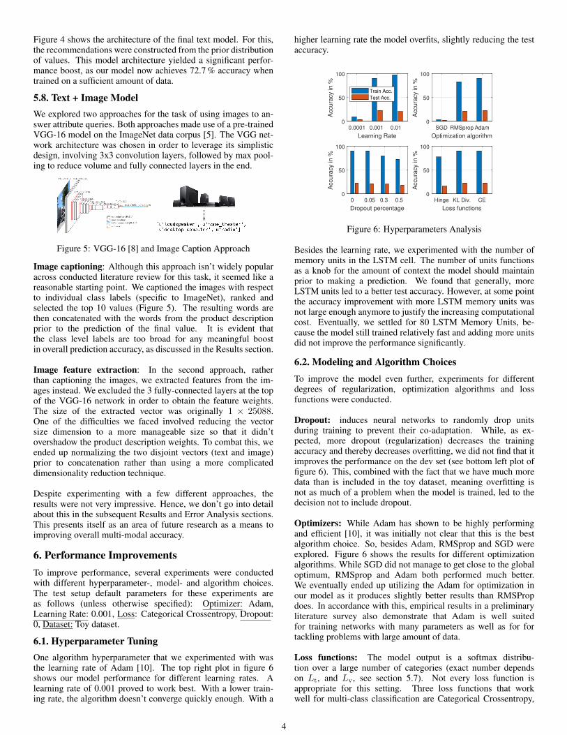
Figure 4 shows the architecture of the final text model. For this,the recommendations were constructed from the prior distributionof values. This model architecture yielded a significant perfor-mance boost, as our model now achieves 72.7 % accuracy whentrained on a sufficient amount of data.

5.8. Text + Image ModelWe explored two approaches for the task of using images to an-swer attribute queries. Both approaches made use of a pre-trainedVGG-16 model on the ImageNet data corpus [5]. The VGG net-work architecture was chosen in order to leverage its simplisticdesign, involving 3x3 convolution layers, followed by max pool-ing to reduce volume and fully connected layers in the end.

Figure 5: VGG-16 [8] and Image Caption Approach

Image captioning: Although this approach isn’t widely popularacross conducted literature review for this task, it seemed like areasonable starting point. We captioned the images with respectto individual class labels (specific to ImageNet), ranked andselected the top 10 values (Figure 5). The resulting words arethen concatenated with the words from the product descriptionprior to the prediction of the final value. It is evident thatthe class level labels are too broad for any meaningful boostin overall prediction accuracy, as discussed in the Results section.

Image feature extraction: In the second approach, ratherthan captioning the images, we extracted features from the im-ages instead. We excluded the 3 fully-connected layers at the topof the VGG-16 network in order to obtain the feature weights.The size of the extracted vector was originally 1 × 25088.One of the difficulties we faced involved reducing the vectorsize dimension to a more manageable size so that it didn’tovershadow the product description weights. To combat this, weended up normalizing the two disjoint vectors (text and image)prior to concatenation rather than using a more complicateddimensionality reduction technique.

Despite experimenting with a few different approaches, theresults were not very impressive. Hence, we don’t go into detailabout this in the subsequent Results and Error Analysis sections.This presents itself as an area of future research as a means toimproving overall multi-modal accuracy.

6. Performance ImprovementsTo improve performance, several experiments were conductedwith different hyperparameter-, model- and algorithm choices.The test setup default parameters for these experiments areas follows (unless otherwise specified): Optimizer: Adam,Learning Rate: 0.001, Loss: Categorical Crossentropy, Dropout:0, Dataset: Toy dataset.

6.1. Hyperparameter TuningOne algorithm hyperparameter that we experimented with wasthe learning rate of Adam [10]. The top right plot in figure 6shows our model performance for different learning rates. Alearning rate of 0.001 proved to work best. With a lower train-ing rate, the algorithm doesn’t converge quickly enough. With a

higher learning rate the model overfits, slightly reducing the testaccuracy.

0.0001 0.001 0.01

Learning Rate

0

50

100

Accura

cy in %

SGD RMSprop Adam

Optimization algorithm

0

50

100

Accura

cy in %

0 0.05 0.3 0.5

Dropout percentage

0

50

100

Accura

cy in %

Hinge KL Div. CE

Loss functions

0

50

100

Accura

cy in %

Train Acc.

Test Acc.

Figure 6: Hyperparameters Analysis

Besides the learning rate, we experimented with the number ofmemory units in the LSTM cell. The number of units functionsas a knob for the amount of context the model should maintainprior to making a prediction. We found that generally, moreLSTM units led to a better test accuracy. However, at some pointthe accuracy improvement with more LSTM memory units wasnot large enough anymore to justify the increasing computationalcost. Eventually, we settled for 80 LSTM Memory Units, be-cause the model still trained relatively fast and adding more unitsdid not improve the performance significantly.

6.2. Modeling and Algorithm ChoicesTo improve the model even further, experiments for differentdegrees of regularization, optimization algorithms and lossfunctions were conducted.

Dropout: induces neural networks to randomly drop unitsduring training to prevent their co-adaptation. While, as ex-pected, more dropout (regularization) decreases the trainingaccuracy and thereby decreases overfitting, we did not find that itimproves the performance on the dev set (see bottom left plot offigure 6). This, combined with the fact that we have much moredata than is included in the toy dataset, meaning overfitting isnot as much of a problem when the model is trained, led to thedecision not to include dropout.

Optimizers: While Adam has shown to be highly performingand efficient [10], it was initially not clear that this is the bestalgorithm choice. So, besides Adam, RMSprop and SGD wereexplored. Figure 6 shows the results for different optimizationalgorithms. While SGD did not manage to get close to the globaloptimum, RMSprop and Adam both performed much better.We eventually ended up utilizing the Adam for optimization inour model as it produces slightly better results than RMSPropdoes. In accordance with this, empirical results in a preliminaryliterature survey also demonstrate that Adam is well suitedfor training networks with many parameters as well as for fortackling problems with large amount of data.

Loss functions: The model output is a softmax distribu-tion over a large number of categories (exact number dependson Lt, and Lv, see section 5.7). Not every loss function isappropriate for this setting. Three loss functions that workwell for multi-class classification are Categorical Crossentropy,

4

KL-Divergence and Categorical Hinge Loss. The effect ofeach of these three loss functions on the model performance isshown in the bottom right plot of Figure 6. In the comparison,Categorical Hinge Loss did not perform as well as the othertwo loss functions. While Categorical Crossentropy slightlyoutperformed KL-Divergence, it is interesting to notice that themodel classified significantly more multi-word values correctwith KL-Divergence compared to Categorical Crossentropy, butfewer single-word values.

7. ResultsPlease refer to Table 1 for a detailed breakdown of the accuracyresults of different experiments on the train and test set, with re-spect to the total accuracy for k = 1.

Exp Specifications Train Test(1) Word2vec cosine similarity 1.5 % 0.5 %(2) T-A-Concatenation 56.5 % 12.4 %(3) Two independent pointers 86.5 % 16.3 %(4) Additional hidden layer 90.7% 23.0 %(5) With image captioning 88.6 % 22.4 %(6) Trained on 342,099 examples 77.7 % 72.7 %

Table 1: Experiment Results for (1) Baseline (2) LSTM-SinglePointer-Net (3) LSTM-Pointer Network (4) Recommendation-Ptr-Net (5) Rec-Ptr-Net + Images (6) Recommendation-Ptr-Net(first four experiments on toy dataset rely on train dataset size:2150 & test dataset size: 544)

The table only shows the most relevant experiments that wereconducted, displayed in the order of experiment evaluation. Thefirst 12 % of accuracy (after baseline) came from using LSTMand a single pointer based on the largest softmax output value.Another 4 % was gained by introducing two independent pointersthat point to the start and the end of the value in the description.Imposing a dependence to these two pointers as well as addingthe recommendation feature yielded 23 % in total. Unfortunately,our approach to include information from images was not verysuccessful. The biggest improvement for the test accuracy wastraining the model on more data, which led to 72.7 % test accu-racy, the highest accuracy we were able to achieve so far.

103

104

105

106

Number of training examples

0

50

100

Accura

cy in %

Train error

Test error

Figure 7: Learning Curve: Variance decreases when the model istrained on more training examples

As shown in figure 7, the model overfits less and generalizesmuch better to the test set when trained on more data. Initially,the variance is high when there is not enough training data andthe gap between train and test error is very large but with moretraining data, this gap becomes significantly smaller.

8. Error AnalysisFor the predictions that are incorrect, there are three main typesof error: a single word close miss, where the predicted word cap-tures the intention but not the right answer, a multi-word close

miss where some of the predicted words are indeed included inthe correct answer and a complete miss, where the prediction isincorrect. Table 2 shows an example for each error category.

Err Attribute Prediction Actual Value(1) batteries included included yes(2) measurements height 1.17 in heel height 1.17 in(3) finish price semi-gloss

Table 2: Error Analysis for (1) Single Word (close miss) (2) MultiWord (close miss) (3) Complete Miss

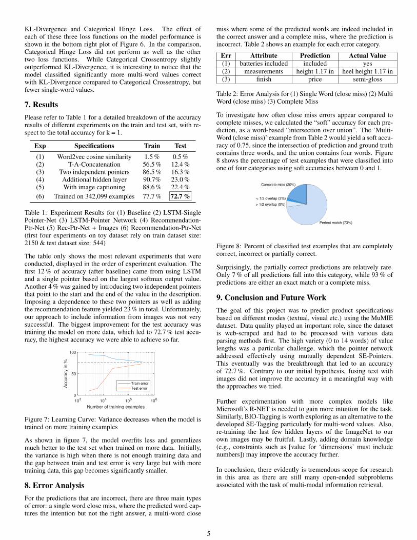
To investigate how often close miss errors appear compared tocomplete misses, we calculated the “soft” accuracy for each pre-diction, as a word-based “intersection over union”. The ‘Multi-Word (close miss)’ example from Table 2 would yield a soft accu-racy of 0.75, since the intersection of prediction and ground truthcontains three words, and the union contains four words. Figure8 shows the percentage of test examples that were classified intoone of four categories using soft accuracies between 0 and 1.

Complete miss (20%)

< 1/2 overlap (2%)

> 1/2 overlap (5%)

Perfect match (73%)

Figure 8: Percent of classified test examples that are completelycorrect, incorrect or partially correct.

Surprisingly, the partially correct predictions are relatively rare.Only 7 % of all predictions fall into this category, while 93 % ofpredictions are either an exact match or a complete miss.

9. Conclusion and Future WorkThe goal of this project was to predict product specificationsbased on different modes (textual, visual etc.) using the MuMIEdataset. Data quality played an important role, since the datasetis web-scraped and had to be processed with various dataparsing methods first. The high variety (0 to 14 words) of valuelengths was a particular challenge, which the pointer networkaddressed effectively using mutually dependent SE-Pointers.This eventually was the breakthrough that led to an accuracyof 72.7 %. Contrary to our initial hypothesis, fusing text withimages did not improve the accuracy in a meaningful way withthe approaches we tried.

Further experimentation with more complex models likeMicrosoft’s R-NET is needed to gain more intuition for the task.Similarly, BIO-Tagging is worth exploring as an alternative to thedeveloped SE-Tagging particularly for multi-word values. Also,re-training the last few hidden layers of the ImageNet to ourown images may be fruitful. Lastly, adding domain knowledge(e.g., constraints such as [value for ‘dimensions’ must includenumbers]) may improve the accuracy further.

In conclusion, there evidently is tremendous scope for researchin this area as there are still many open-ended subproblemsassociated with the task of multi-modal information retrieval.

5

ContributionsDuring almost all of our coding and writeup sessions we sat to-gether in one conference room to ensure everyone is contribut-ing an equal amount to the project. We often split the work intoseveral sub-problems that were tackled individually (divide andconquer) and later merged in our private Bitbucket repository.

References[1] P. Anderson, X. He, C. Buehler, D. Teney, M. Johnson,

S. Gould, and L. Zhang. Bottom-up and top-down at-tention for image captioning and vqa. arXiv preprintarXiv:1707.07998, 2017.

[2] S. Antol, A. Agrawal, J. Lu, M. Mitchell, D. Batra,C. Lawrence Zitnick, and D. Parikh. Vqa: Visual ques-tion answering. In Proceedings of the IEEE InternationalConference on Computer Vision, pages 2425–2433, 2015.

[3] D. Bahdanau, K. Cho, and Y. Bengio. Neural machinetranslation by jointly learning to align and translate. arXivpreprint arXiv:1409.0473, 2014.

[4] T. Baltrusaitis, C. Ahuja, and L.-P. Morency. Multimodalmachine learning: A survey and taxonomy. arXiv preprintarXiv:1705.09406, 2017.

[5] J. Deng, W. Dong, R. Socher, L.-J. Li, K. Li, and L. Fei-Fei. Imagenet: A large-scale hierarchical image database.In Computer Vision and Pattern Recognition, 2009. CVPR2009. IEEE Conference on, pages 248–255. IEEE, 2009.

[6] L.-Y. Deng. The cross-entropy method: a unified approachto combinatorial optimization, monte-carlo simulation, andmachine learning, 2006.

[7] D. Elworthy. Question answering using a large nlp system.In TREC, 2000.

[8] D. Frossard. Vgg in tensorflow. University of Toronto, 2016.

[9] S. Hochreiter and J. Schmidhuber. Long short-term mem-ory. Neural computation, 9(8):1735–1780, 1997.

[10] D. Kingma and J. Ba. Adam: A method for stochastic opti-mization. arXiv preprint arXiv:1412.6980, 2014.

[11] A. Lazaridou, N. T. Pham, and M. Baroni. Combining lan-guage and vision with a multimodal skip-gram model. arXivpreprint arXiv:1501.02598, 2015.

[12] L. Marquez, P. Comas, J. Gimenez, and N. Catala. Seman-tic role labeling as sequential tagging. In Proceedings ofthe Ninth Conference on Computational Natural LanguageLearning, pages 193–196. Association for ComputationalLinguistics, 2005.

[13] P. Rajpurkar, J. Zhang, K. Lopyrev, and P. Liang. Squad:100,000+ questions for machine comprehension of text.arXiv preprint arXiv:1606.05250, 2016.

[14] K. Simonyan and A. Zisserman. Very deep convolutionalnetworks for large-scale image recognition. arXiv preprintarXiv:1409.1556, 2014.

[15] B. Steiner. Tensorflow word2vec tutorial. https://github.com/tensorflow/tensorflow/blob/master/tensorflow/examples/tutorials/word2vec/word2vec_basic.py,2015.

[16] M. Tan, C. d. Santos, B. Xiang, and B. Zhou. Lstm-based deep learning models for non-factoid answer selec-tion. arXiv preprint arXiv:1511.04108, 2015.

[17] O. Vinyals, M. Fortunato, and N. Jaitly. Pointer networks. InAdvances in Neural Information Processing Systems, pages2692–2700, 2015.

[18] S. Wang and J. Jiang. Learning natural language inferencewith lstm. arXiv preprint arXiv:1512.08849, 2015.

[19] S. Wang and J. Jiang. Machine comprehension using match-lstm and answer pointer. arXiv preprint arXiv:1608.07905,2016.

[20] Z. Yang, X. He, J. Gao, L. Deng, and A. Smola. Stackedattention networks for image question answering. In Pro-ceedings of the IEEE Conference on Computer Vision andPattern Recognition, pages 21–29, 2016.

[21] Y. Zhu, O. Groth, M. Bernstein, and L. Fei-Fei. Visual7w:Grounded question answering in images. In Proceedingsof the IEEE Conference on Computer Vision and PatternRecognition, pages 4995–5004, 2016.

6