Multi-layer injection moulding of oil-filled rubber dampers

Swartjes, F.H.M.

Published: 01/01/1995

Document VersionPublisher’s PDF, also known as Version of Record (includes final page, issue and volume numbers)

Please check the document version of this publication:

• A submitted manuscript is the author's version of the article upon submission and before peer-review. There can be important differencesbetween the submitted version and the official published version of record. People interested in the research are advised to contact theauthor for the final version of the publication, or visit the DOI to the publisher's website.• The final author version and the galley proof are versions of the publication after peer review.• The final published version features the final layout of the paper including the volume, issue and page numbers.

Link to publication

General rightsCopyright and moral rights for the publications made accessible in the public portal are retained by the authors and/or other copyright ownersand it is a condition of accessing publications that users recognise and abide by the legal requirements associated with these rights.

• Users may download and print one copy of any publication from the public portal for the purpose of private study or research. • You may not further distribute the material or use it for any profit-making activity or commercial gain • You may freely distribute the URL identifying the publication in the public portal ?

Take down policyIf you believe that this document breaches copyright please contact us providing details, and we will remove access to the work immediatelyand investigate your claim.

Download date: 15. Jul. 2018

Multi-layer iiijection moulding of oil-filled rubber dampers

F.H.M. Swartjes

WFW report 95.096

Supervised by: d r h . G.W.M. Peters and ir. L. Kleintjes Faculty of Mechanical Engineering

Eindhoven University of Technology July 1995

Contents .. Summary 11

1 Introduction 1 1 . 1 Multicomponent injection moulding . . . . . . . . . . . . . . . . . . . . . . . . . 1 1.2 Oil-filled rubber dampers . . . . . . . . . . . . . . . . . . . . . . . . . . . . . . . 1

2 Experimental and numerical methods 2 2.1 Experimental setup . . . . . . . . . . . . . . . . . . . . . . . . . . . . . . . . . . . 2

2.1.1 Dimensions of the product . . . . . . . . . . . . . . . . . . . . . . . . . . . 2 2.1.2 Equipment . . . . . . . . . . . . . . . . . . . . . . . . . . . . . . . . . . . 2 2.1.3 Working method . . . . . . . . . . . . . . . . . . . . . . . . . . . . . . . . 4

2.2 Numerical methods . . . . . . . . . . . . . . . . . . . . . . . . . . . . . . . . . . . 4 2.2.1 Particle tracking . . . . . . . . . . . . . . . . . . . . . . . . . . . . . . . . 4 2.2.2 Balance equations . . . . . . . . . . . . . . . . . . . . . . . . . . . . . . . 5 2.2.3 Boundary conditions . . . . . . . . . . . . . . . . . . . . . . . . . . . . . . 6 2.2.4 Numerical calculation . . . . . . . . . . . . . . . . . . . . . . . . . . . . . 7

3 Materials a 4 Experimental and numerical results 8

4.1 Numerical results . . . . . . . . . . . . . . . . . . . . . . . . . . . . . . . . . . . . 8 4.2 Experimental results . . . . . . . . . . . . . . . . . . . . . . . . . . . . . . . . . . 10

5 Conclusions and recommendations 11 5.1 Conclusions . . . . . . . . . . . . . . . . . . . . . . . . . . . . . . . . . . . . . . . 11 5.2 Recommendations . . . . . . . . . . . . . . . . . . . . . . . . . . . . . . . . . . . 11

Appendix A: Volume of the product 17

Appendix B: Listings 18 B.l Main program . . . . . . . . . . . . . . . . . . . . . . . . . . . . . . . . . . . . . . 18 B.2 Input for meshgeneration . . . . . . . . . . . . . . . . . . . . . . . . . . . . . . . . 47 B.3 Input for the solver . . . . . . . . . . . . . . . . . . . . . . . . . . . . . . . . . . . 49 B.4 Input for postprocessing . . . . . . . . . . . . . . . . . . . . . . . . . . . . . . . . . 52

Appendix C: Slipvelocities 53

Appendix D: Upwinding 55

References 56

1

Summary

This study is on multicomponent injection moulding. The main goal of this work is the use of the multi-layer injection moulding process for producing oil-filled dampers. A relatively simple tool is created to determine the feasibility of the process itself. This tool has not been designed for a real production process, but only has to produce few dampers. Numericai simuiations of the filiing of the mould have been carried out with the ñnite element package SEPRAN. At the inflow the rubber and oil are labelled. During filling of the mould, the labels are followed by solving a convective equation and the air is modelled at the boundaries with a slip condition. The air slips with the 'mean' velocity of the front. I t is difficult and time- consuming to predict the right slipvelocities. The results are satisfactory when the velocities are chosen in the right range. The sequential injection gives better results than the combined injection in terms of the oildistribution in the product. The injection of oil with the experiments is not controllable and therefore not reproduceble. Some of the problems are that the filling of the mould is asymmetrically and that , when the mould is filled completely, rubber is pressed into the oil feeding.

11

1 Introduction

1.1 Multicomponent injection moulding

The injection moulding process is a flexible production method to fabricate plastic parts in series, characterized by the ability to realize complex shaped, highly integrated products in small cycle times. The high flexibility of the injection moulding technique can be extended with the possibility of combining different materials within one produkt, each with its own specific properties. With a multicomponent (or multilayer) injection moulding technique a layered structure of two or more components can be realized within a thin-walled product. The geometry of the layers in the product depends mainly on the position of the gate, the geometry of the nozzle and the sequence of injection (simultaneously and/or sequential). An injection moulding machine mainly consists of two parts: an injection and a clamping unit. Granulated polymer is supplied by a hopper to the feeding part of the rotating extruder screw. The rotating of the extruder screw causes the granulate to move through the heated extruder barrel. Heat, generated by the heating elements and by the screw rotation, causes the granulate to plasticize. When sufficient material has been plasticized, the screw acts as a piston and pushes the melt through a nozzle and runner system into the mould cavity. The clamping unit supports the two mould halves and prevents the mould from opening despite of the high pressure that occurs during the process. The moulding cycle can be divided into three stages: the injection, the packing and holding, and the cooling stage. First the molten polymer is injected in the mould (injection stage). After complete filling of the cavity, extra makerial will be added to compensate for shrinkage (packing and holding stage). At the moment the gate is sealed, compensation for shrinkage is no longer possible and the cooling stage starts. When the temperature has decreased below the ejection temperature, the mould is opened and the produkt can be ejected. In this study the multicomponent injection moulding process will be used t o make oil-filled rubber dampers.

1.2 Oil-filled rubber dampers

Oil-filled rubber dampers are used for the suspension of the laser module inside an outdoor CD-player. The CD-mechanism is damped with four oil-filled rubber dampers. Such a damper has excellent performance in terms of damping and reduction characteristics at high frequencies (de Geus [i]). The current used oil-filled rubber damper in the outdoor CD-players, has a high cost-prize due to the used production method. The process includes multiple production cycles. The first production cycle is the injection moulding of the rubber cup. In a second cycle the cup is filled with the silicon oil, and in the last cycle a rubber disc is glued on the cup t o close the damper. Miniaturization of outdoor CD-applications demands that the oil-filled rubber damper will be reduced in volume substantially in near future. The multilayer injection moulding process will be used to produce oil-filled rubber dampers. It is vital t ha t the complete process is reproducible. Geometry variations, like the thickness of the oil layer, have large effects on the dynamic characteristics of the damper. To enhance flow visualization and to keep the mould within reasonable filling measures (not to small) the dimensions of the damper are made larger with respect to the current used oil-filled rubber dampers. The dynamic characteristics are of minor importance in this study. Further on, the multi-layer structure may not exist in the injection channels after complete filling of the mould.

1

The oil is a fluid at room temperature, so the damper would not be closed. The ultimate goal of simulation of the injection moulding process, is to predict the process conditions given the required product properties. With a numerical simulation in the finite element package SEPRAN (Segal [3]) the time and duration of injection can be determined. By simulating the injection moulding process for different times and different durations of the injection of the oil, the process conditions for the experiments can be determined. in chapter 2 of this report the experimentai and numericai setup will be discussed. The materials used are described in chapter 3. The numerical results of two different kinds of injection are discussed in chapter 4. Also the results of the experiments are discussed in this chapter. Finally, chapter 5 summarizes the main results and gives suggestions for future research.

2 Experimental and numerical methods

2.1 Experimental setup

2.1.1 Dimensions of the product

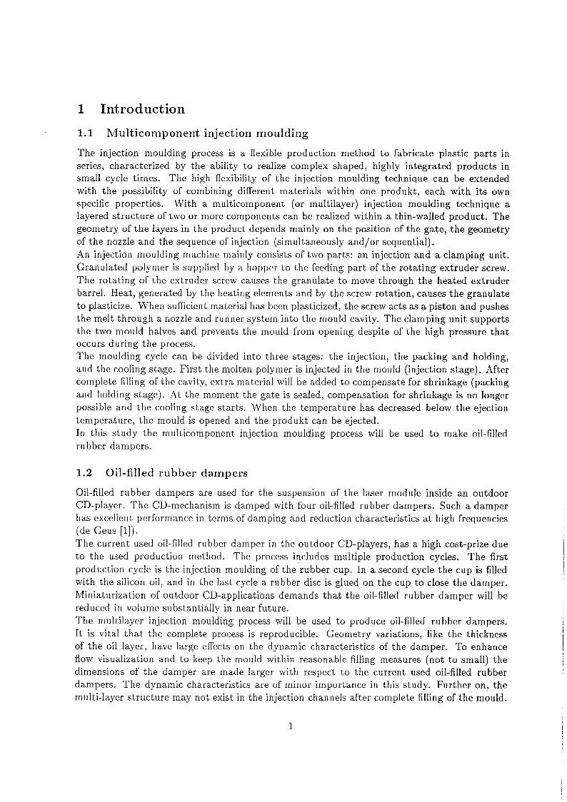
The oil-filled rubber damper for the experimental setup is made somewhat larger as the conven- tional oil-filled rubber damper, as stated before (see Figure 1). The experiments are primarily

26

Figure 1: Dimensions of the product

focused on the feasibility of the process itself. Down sizing the product can be done when the process has been proven feasible. Figure 1 shows that the walls of the product are not per- pendicular to the top of the product. This angle of 6.0" is necessary t o ease the remove of the product. The exact volume of the product is equal to 10.S89 [rnrn3] (see Appendix A). The maximum injectionvolume of oil is about 5659 [mrn3]. With the experiments and the numerical calculations these values have been taken into account.

2.1.2 Equipment

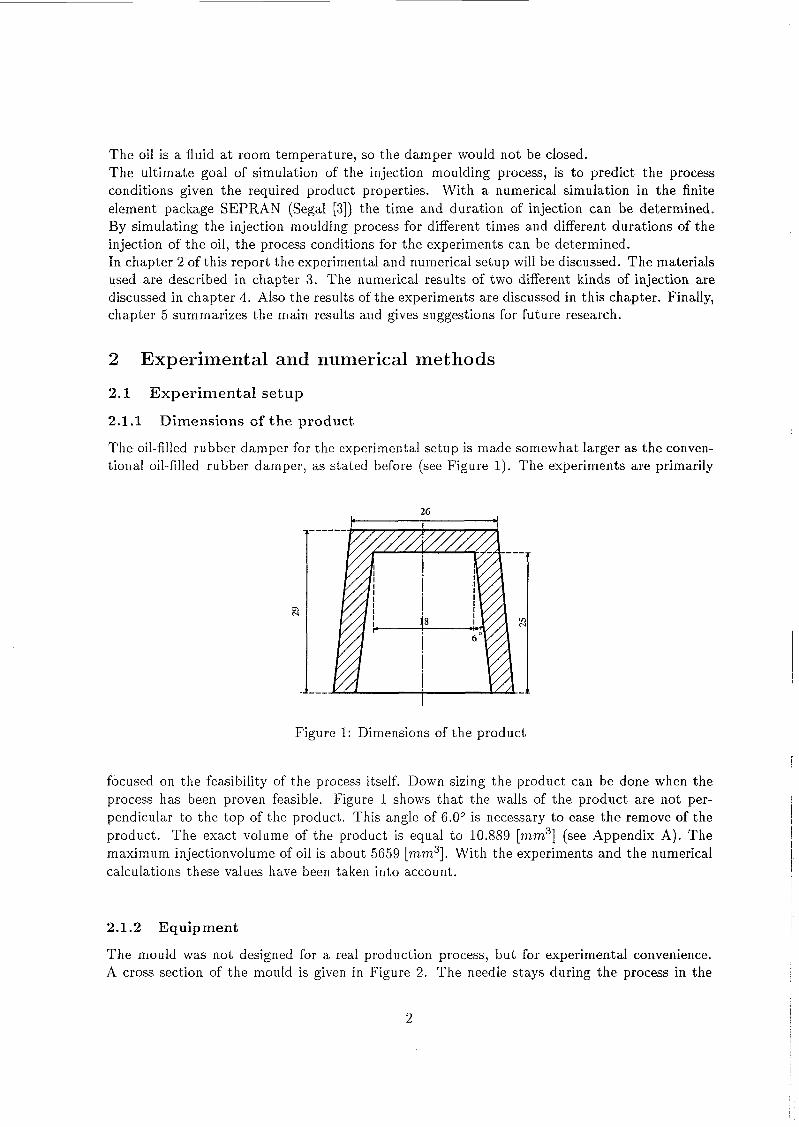
The mould was not designed for a real production process, but for experimental convenience. A cross section of the mould is given i n Figure 2. The needle stays during the process in the

2

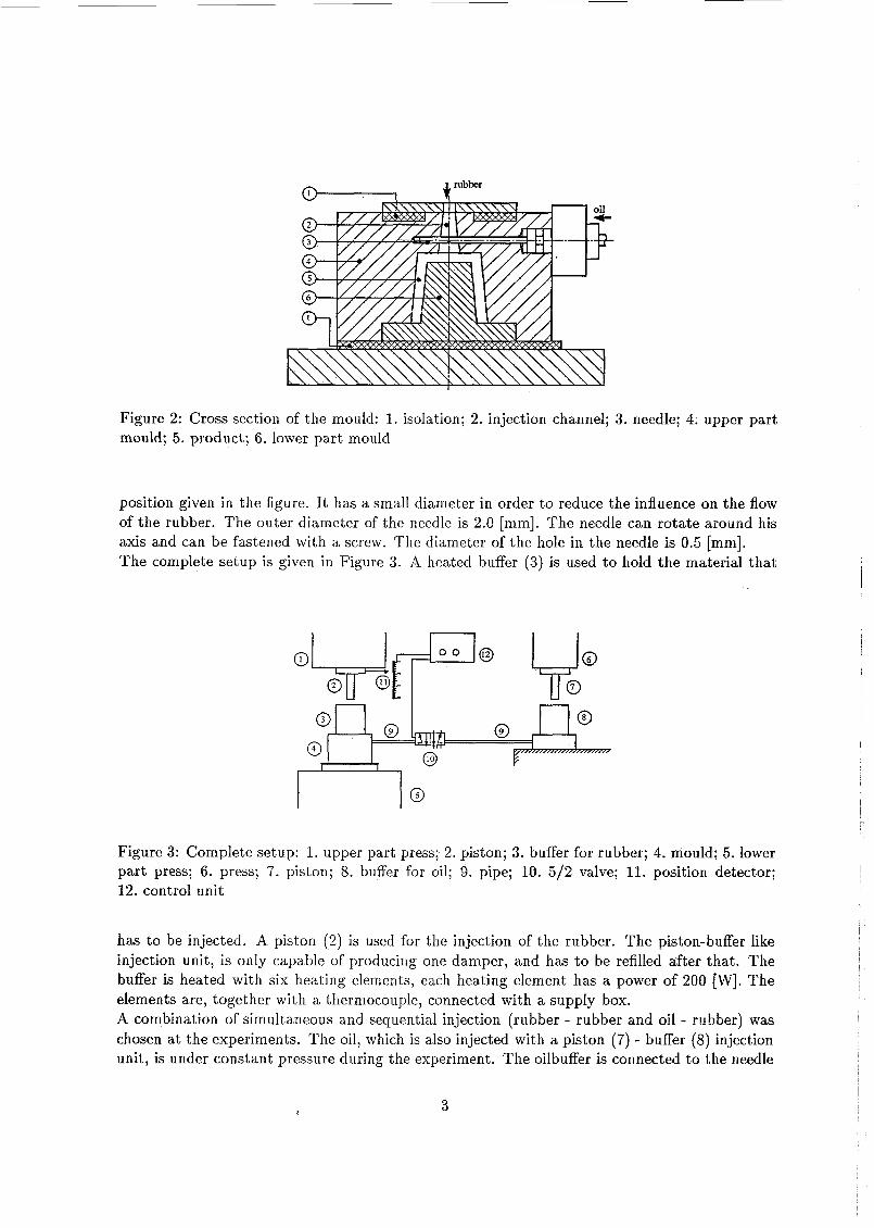
Figure 2: Cross section of the mould: 1. isolation; 2. injection channel; 3. needle; 4. upper part mould; 5 . product; 6. lower part mould

position given in the figure. It has a small diameter in order t o reduce the influence on the flow of the rubber. The outer diameter of the needle is 2.0 [mm]. The needle can rotate around his axis and can be fastened with a screw. The diameter of the hole in the needle is 0.5 [mm]. The complete setup is given in Figure 3. A heated buffer (3) is used t o hold the material that

Figure 3: Complete setup: 1. upper part press; 2. piston; 3. buffer for rubber; 4. mould; 5 . lower part press; 6. press; 7. piston; 8. buffer for oil; 9. pipe; 10. 5/2 valve; 11. position detector; 12. control unit

has t o be injected. A piston (2) is used for the injection of the rubber. The piston-buffer like injection unit, is only capable of producing one damper, and has t o be refilled after that . The buffer is heated with six heating elements, each heating element has a power of 200 [W]. The elements are, together with a thermocouple, connected with a supply box. A combination of simultaneous and sequential injection (rubber - rubber and oi! - rubber) was chosen at the experiments. The oil, which is also injected with a piston (7) - buffer (8) injection unit, is under constant pressure during the experiment. The oilbuffer is connected t o the needle

3

with a pipe (9) and a valve (10). The valve and the position detector (11) of the rubber injection unit, are connected with a control unit (12) which is used to adjust the injection of oil. Two knobs with a scale [O-101, corresponding to the (maximum) stroke of the piston (50 [mm]), are used for that .

2.1.3 W o r k i n g method

The rubber, Hytrel, is available in grains. The grains are pressed in plates at a temperature cf 230°C. First the grains are melted and after that the pressure is raised after each five minutes (the adjusted compressional forces are: 1, 2, 5, 10, and 20 [kN]). The plates are cut in small blocks from which the slices are made at a lathe. These slices fit in the buffer. The different actions during the experiment are:

o clean the mould with a brass brush and acetone

o fill the buffer with rubber and (if necessary) fill the oilbuffer

o press the mould against the buffer

o position the needle. The needle has to be fa.stened and in the right direction before material is injected.

o press the piston against the rubber

o heat the buffer

o choose the begin and end of the injection of oil

o when the buffer is on temperature wait for fifteen minutes

o inject the rubber and oil

o cool down the mould with air or wait for a time and take out the product after the pressure has been taken of the mould

2.2 Numerical methods

2.2.1 Par t i c l e t r ack ing

In order to realize the desired product geometry in the mold, knowledge of the time and dura- tion of injection of the different components is required. Using the conservation of identity, the position of material injected at arbitrary moments can be determined. In this particle tracking technique material particles are defined by their unique identity (e.g. material, colour, place and time of injection). The particles are abstract, distinct points in the flow that have to be followed in time and space. By following the particles through the flow domain the material distribution is known. Zoetelief [2] has shown tha t the conservation of identity method can be applied succesfully to track the material interfaces. Those interfaces that occur in the mould filling simulations, can be modelled with a jump of the material properties (e.g. q or p ) at the inferfaces. In this study, two different interfaces can be distinguished. First, there exists an interface be- tween the rubber melt and the air during the filling. The second type of interface is the one

I

I Ï

4

between the rubber and the oil. The filling of the mould is assumed to be isothermal, so there is no interface between a solid and liquid layer of rubber. Both interfaces are modelled with a discontinuity in the viscosity. They are approximated by continuous functions with a steep gradient. The maximum steepness is controlled by the local mesh size and the order of the element. A major influence on the final particle distribution throughout the product is the so-called fountain Bow. In Bows with one or more Îree boundaries and a no-siip condition at the walis, fluid elements adjacent to the moving front experience this phenomenon. The fluid near the center moves at a higher speed than the local average speed across the channel. When the fluid reaches the front, it spreads towards the walls. Material injected later in the injection period may breakthrough previously injected material. So breakthrough of the second injected material through the first injected materia.1 is completely governed by the fountain effect at the flow front. Breakthrough may not occur with the production of the oil filled rubber dampers. The oil must be completely surrounded by the rubber.

2.2.2 Balance equatioiis

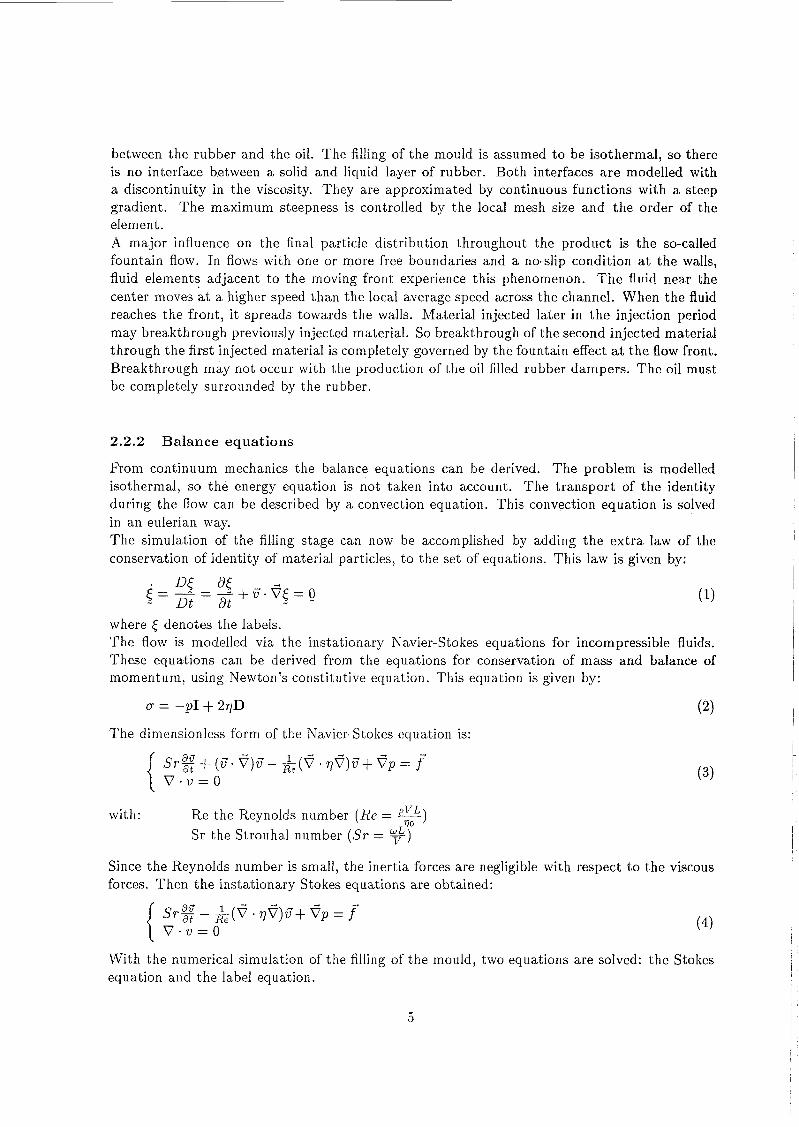
From continuum mechanics the balance equations can be derived. The problem is modelled isothermal, so the energy equation is not taken into account. The transport of the identity during the flow can be described by a convection equation. This convection equation is solved in an eulerian way. The simulation of the filling stage can now be accomplished by adding the extra law of the conservation of identity of material paprticles, to the set of equations. This law is given by:

where E denotes the labels. The flow is modelled via the instationary Navier-Stokes equations for incompressible fluids. These equations can be derived from the equations for conservation of mass and balance of momentum, using Newton’s constitutive equation. This equation is given by:

O = -PI + 27D (2)

The dimensionless form of the Navier-Stokes equation is:

with: Re the Reynolds number (Re = e) Sr the Strouhal number ( S r = 9)

Since the Reynolds number is small, the inertia forces are negligible with respect t o the viscous forces. Then the instationary Stokes equations are obtained:

With the numerical simula.tion of the filling of the mould, two equations are solved: the Stokes equation and the la.bel equation.

I c

5

2.2.3 B o u n d a r y condi t ions

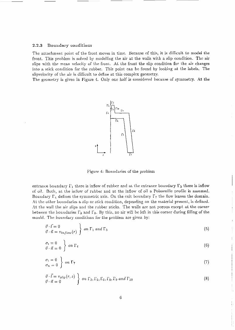
The attachment point of the front moves in time. Because of this, it is difficult t o model the front. This problem is solved by modelling the air at the walls with a slip condition. The air slips with the mean velocity of the front. At the front the slip condition for the air changes into a stick condition for the rubber. This point can be found by looking at the labels. The slipvelocity of the air is difficult to define at this complex geometry. The geometry is given in Figure 4. Only one half is considered because of symmetry. At the

r2

r4

I- r

Figure 4: Boundaries of the problem

entrance boundary rl there is inflow of rubber and a t the entrance boundary I's there is inflow of oil. Both, at the inflow of rubber and at the inflow of oil a Poisseuille profile is assumed. Boundary r4 defines the symmetric axis. On the exit boundary I'7 the flow leaves the domain. At the other boundaries a slip or stick condition, depending on the material present, is defined. At the wall the air slips and the rubber sticks. The walls are not porous except at the corner between the boundaries I'S and r g . By this, no air will be left in this corner during filling of the mould. The boundary conditions for the problem are given by:

on ri and r3 ü.t, o 21 n = Vinf iow ( r ) - 4

6

Both, the boundaries of the label equation and the Stokes equation are time-dependent. The boundary conditions of the Stokes equation depend on the position of the front. The two materials can be injected sequential (rubber - oil - rubber) or a combination of simultaneous and sequential (rubber - rubber and oil - rubber). The label of boundary r3 has only the label of oil when oil is injected.

2.2.4 N u m e r i c a l calculat ion

ï'he calculation of the filling of the mould is executed in the following steps:

o solve the label equation with the velocities of the previous time step

o determine the time-dependent boundary conditions for the Stokes equation based on the labels of the boundary nodes

o solve the Stokes equation

o determine the viscosity based on the labels

o generate output for postprocessing

The program and the input for the preprocessor, solver and postprocessor can be found in Appendix B.

3 Materials

The damper consists of two materials: a rubber and an oil. The rubber component of the conventional oil-filled rubber damper is butyl rubber. Butyl rubber is a vulcanized rubber, and therefore not tliermo-reversible. To simplify the experiments, Hytrel 6356, is used. Hytrel 6356 is a thermoplastic polymer. So Hytrel does not vulcanize, but it behaves like a vulcanized rubber. Hytrel is a hygroscopic material, so the time during which Hytrel is exposed to atmospheric moisture must be kept minimum. The resin should be dried for 2-3 hours at 105°C - 120"C, if exposure to ambient air exceeds one hour. The viscosity of Hytrel was measured using small amplitude oscillatory shear experiments on a Rheometrics Dynamics Spectrometer RDS-11. The parallel plate geometry was used. The sample geometry was: ~ 2 5 x 1.374 [mm]. The data are measured as a function of the frequency at different temperatures between 215°C and 275°C. The melting temperature of Hytrel is equal t o 211°C. The dynamic viscosity of Hytrel is about 50 [Pas] at a temperature of 250°C. The experiments are done at this temperature. The oil in the damper is a silicon or polybutene oil. Silicon oils are build EP of non-cross linked polydimethylsiloxane elastomeric chains. They mainly behave viscous and are water free fluids. The silicon oils used are produced by Waclter Chemie. The silicon oils AK are available in a wide viscosity range. For damping applications, silicon oils with a viscosity of q > 10 [Pas] are of real importance (de Geus [i]). The valve, which regulate the injection of oil in the mould, is not able to resist high pressures, which is necessary to press a higly viscous oil through the pipes. The valve opens when the pressure is too high. For this reason the viscosity of the oil may not be taken too high. A prediction of the viscosity of the oil can be determined. The maximum presstire the valve can stand is about 27.1 . lo5 [Pas]. The pressure necessary t o press the oil through the pipe has

7

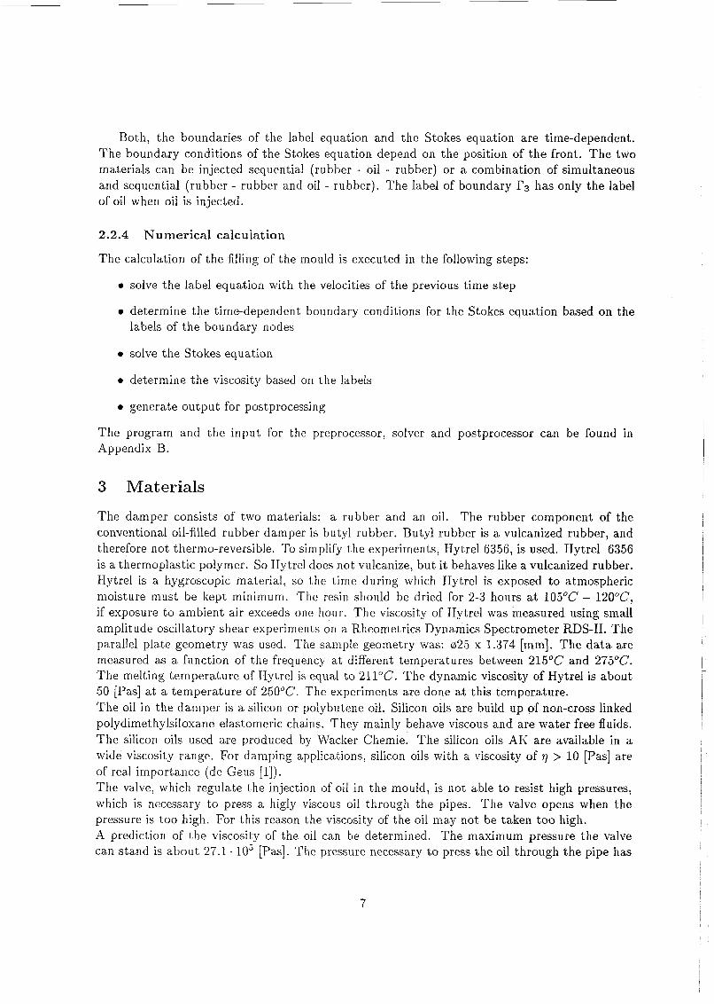
t o be lower than this value. It is assumed that the volumeflow in the straight pipes satisfy the relation of Hagen-Poiseuille:

q [Pas] 0.1 1 .o

where u, is the mean velocity, q is the viscosity, 2 is the pressuregradient and R the radius of the pipe. The pressure difference over a pipe with length L is equal t o

AP [Pal

5.4. io3 7.84. io4 8 . 3 8 . io4 5.4. io4 7.84. io5 s.38 - i o5

supply pipe needle total

The supply pipe has a length of 0.977 [m] and an inner radius of 2.0 [m]. The needle has a length of 5.5 . [m]. The prescribed flow of oil is equal to 3.5 - 10-7[rn3s-1]. The pressure drop is calculated for two different viscosities. The results are given in Table 1. The va,lue of the pressure difference is mainly influenced by the needle.

[m] and an inner radius of 5.0

material air

q [Pas] 1.0 - 10-1

Table 1: Pressure drop

Both Wacker AI(100 and Wacker AK1000 satisfy the condition above. The dampers which have been made, are filled with AK100 (7 = 0.1 [Pas]).

4 Experimental and numerical results

4.1 Numerical results

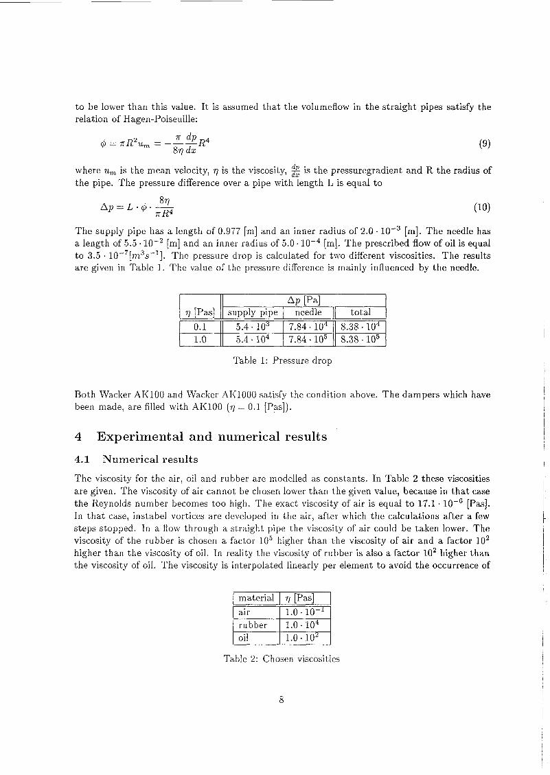
The viscosity for the air, oil and rubber are modelled as constants. In Table 2 these viscosities are given. The viscosity of air cannot be chosen lower than the given value, because in that case the Reynolds number becomes too high. The exact viscosity of air is equal t o 17.1 [Pas]. In tha t case, instabel vortices are developed in the air, after which the calculations after a few steps stopped. In a flow through a straight pipe the viscosity of air could be taken lower. The viscosity of the rubber is chosen a factor lo5 higher than the viscosity of air and a factor lo2 higher than the viscosity of oil. In reality the viscosity of rubber is also a factor lo2 higher than the viscosity of oil. The viscosity is interpolated linearly per element to avoid the occurrence of

Table 2: Chosen viscosities

8

unrealistic values in the integration points. This may occur at the two material interfaces due to the quadratic shape functions of the elements used. The numerical simulations are performed using a finite element mesh consisting of 1472 quadratic triangular elements as is depicted in Figure 5. The fine mesh is necessary to visualize the fountainflow and to determine the front of the rubber. The applied boundary conditions are already given in Figure 4. Because of symmetry only one half of the geometry is modelled. The slipvelocities of the air on the boundaries are described in Appendix C.

The Stokes equation with the incompressibility constraint is solved with a, penalty method. The calculation of the velocity and the pressure are uncoupled and the incompressibility con- straint is taken into account in the Stokes equation with a penalty parameter after discretization of equation (4) and applying the Galerkin formulation. The velocity field is calculated by a Pi- card iteration method (successive substitution) every time step. The rate of convergence of Picard is linear (see also van Steenhoven [4]). For the solution of the particle tracking problem, the Streamline Upwind Petrov-Galerkin finite element method is applied using the same mesh as in the Stokes problem. T h e SUPG method provides stable solutions in case of convection dominated flows with discontinuities in the solu- tion as may occur in the particle tracking problem. The classical upwind scheme is used ( C = 1 see Appendix D). From all the types of upwinding within the SUPG method this scheme gives the least accurate, but smoothest results. The time integration is carried out with an Euler implicit scheme (6' = 1). This scheme applied to equation (1) leads to

material rubber

oil

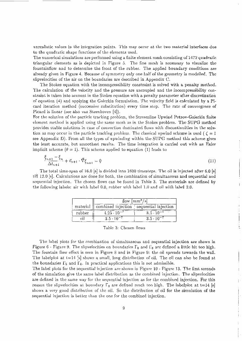
The total time-span of 16.0 [SI is divided into 1600 timesteps. The oil is injected after 6.0 [s] till 12.0 [Is]. Calculations are done for both, the combination of simultaneous and sequential and sequential injection. The chosen flows can be found in Table 3. The materials are defined by the following labels: air with label 0.0, rubber with label 1.0 and oil with label 2.0.

flow [mm3/s]

4.25.10-7 8.5.10-7 3.5.10-7 3.5.10-7

combined injection sequential injection

Table 3: Chosen flows

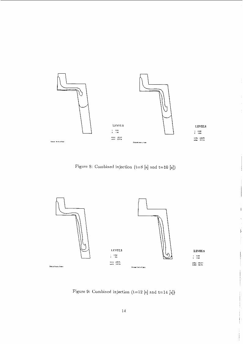
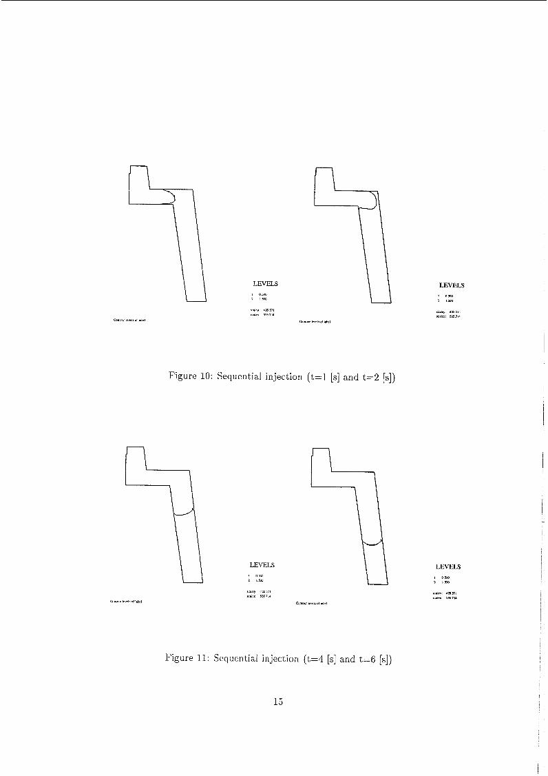
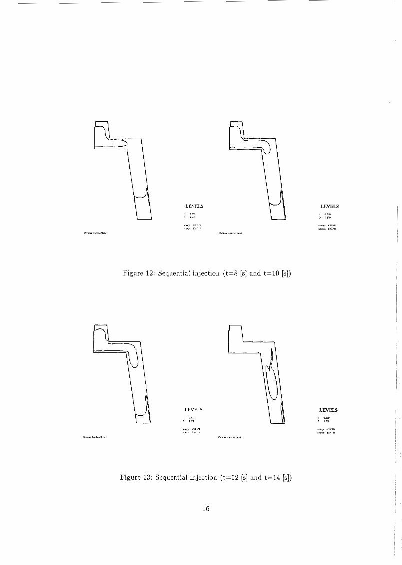
The label plots for the combination of simultaneous and sequential injection are shown in Figure 6 - Figure 9. The slipvelocities on boundaries r6 and I's are defined a little bit too high. The fountain flow effect is seen in Figure S and in Figure 9: the oil spreads towards the wall. The labelplot at t=14 [s] shows a small, long distribution of oil. The oil can also be found a t the boundaries I's and r6. In practical applications this is not admissible. The label plots for the sequential injection are shown in Figure 10 - Figure 13. T h e first seconds of the simulation give the same label distribution as the combined injection. The slipvelocities are defined in the same way for the sequential injection as for the combined injection. For this reason the slipvelocities a t boundary I's are defined much too high. The labelplot at t=14 [SI shows a very good distribution of the oil. So the distribution of oil for the simulation of the sequential injection is better than the one for the combined injection.

9

4.2 Experimental results

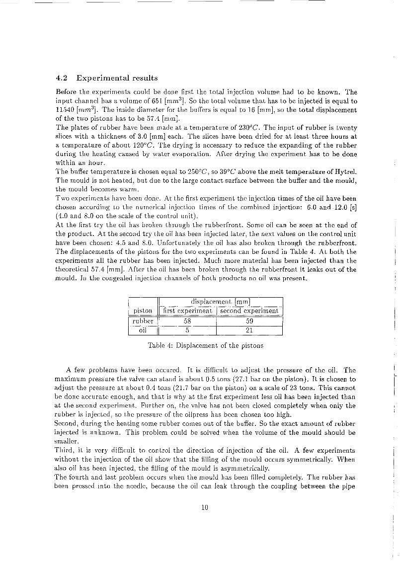
Before the experiments could be done first the total injection volume had t o be known. The input channel has a volume of 651 [mm’]. So the total volume that has to be injected is equal t o 11540 [mm’]. The inside diameter for the buffers is equal t o 16 [mm], so the total displacement of the two pistons has to be 57.4 [mm]. The plates of rubber have been made at a temperature of 230°C. The input of rubber is twenty slices with a thickness of 3.0 [mm] each. The slices have been dried €or at !east three hours at a temperature of about 120°C. The drying is necessary to reduce the expanding of the rubber during the heating caused by water evaporation. After drying the experiment has to be done within an hour. The buffer temperature is chosen equal to 250”C, so 39°C above the melt temperature of Hytrel. The mould is not heated, but due to the large contact surface between the buffer and the mould, the mould becomes warm. Two experiments have been done. At the first experiment the injection times of the oil have been chosen according to the numerical injection times of the combined injection: 6.0 and 12.0 [s] (4.0 and 8.0 on the scale of the control unit). At the first try the oil has broken through the rubberfront. Some oil can be seen at the end of the product. At the second try the oil has been injected later, the next values on the control unit have been chosen: 4.5 and 8.0. Unfortunately the oil has also broken through the rubberfront. The displacements of the pistons for the two experiments can be found in Table 4. At both the experiments all the rubber has been injected. Much more material has been injected than the theoretical 57.4 [mm]. After the oil has been broken through the rubberfront i t leaks out of the mould. In the congealed injection channels of both products no oil was present.

piston rubber

oil

displacement [mm] first experiment second experiment

58 59 5 21

A few problems have been occured. It is difficult to adjust the pressure of the oil. The maximum pressure the valve can stand is about 0.5 tons (27.1 bar on the piston). It is chosen t o adjust the pressure a t about 0.4 tons (21.7 bar on the piston) on a scale of 23 tons. This cannot be done accurate enough, and that is why at the first experiment less oil has been injected than at the second experiment. Further on, the valve has not been closed Completely when only the rubber is injected, so the pressure of the oilpress has been chosen too high. Second, during the heating some rubber comes out of the buffer. So the exact amount of rubber injected is unknown. This problem could be solved when the volume of the mould should be smaller. Third, it is very difficult to control the direction of injection of the oil. A few experiments without the injection of the oil show that the filling of the mould occurs symmetrically. When also oil has been injected, the filling of the mould is asymmetrically. The fourth and last problem occurs when the mould has been filled completely. The rubber has been pressed into the needle, because the oil can leak through the coupling between the pipe

r

10

and the valve.

5 Conclusions and recommendations

5.1 Conclusions

The numerical calculations show that the distribution of oil for the simulation of the sequential injection is better than the one for the combined injection. The combined injection gives a wider distribution of oil, but oil can be found near the innerwall and the oil approaches the rubberfront at the end of the simulation. The real viscosity of air could not be implemented in the program, because in tha t case the Reynolds number becomes too high. The method with the slip of air at the walls give only good results when the right slipvelocities are chosen. For a complex geometry this is quite difficult and time-consuming. In the future new elements will be available which generate the right slipvelocity. The fine mesh is necessary to determine the front of the rubber and to visualize the fountain flow. The fountain flow effect is visualized a t the combined injection. The injection of oil at the experiments is not controllable and reproduceble. The valve can not stand high pressures, so an oil with a low viscosity has to be used. The filling of the mould is asymmetrically when also oil is injected. The theoretical, vertical injection of the oil can not be adjusted accurately. This could be the reason for the asymmetrical injection. When the mould is completely filled, rubber is pressed into the needle. The vicosity of the oil is too low by which the oil is pressed through leaks a t the couplings. Drying of the rubber slices is necessary to reduce the expanding of the rubber during the heating. During heating of the buffer some rubber leaks out of the buffer. The buffer has t o be filled almost completely to ensure that the mould will be filled completely.

5.2 Recommendations

To appoximate the reality more, the program has to be extended with the energy equation and models for the viscosity. The premature congelation of rubber could have a great influence on the profiles of the flow. In the future the new element could be implemented in the program. The volume of the mould should be made smaller. In that case less slices are needed for an experiment and the leaking of the rubber out of the buffer will be reduced. The injection of oil has to be changed to inject also oils with a higher viscosity than the oil used (7 = 0.1 [pas]). The 5/2 valve has to be replaced by a valve which resists the high pressures necessary to press the oil with the higher viscosity through the pipe and needle. Those oils will leak less at the couplings between the pipes and the valve. In that case less rubber will be pressed into the needle. Also experiments should be done with the sequential injection, because the numerical results give a well defined labeldistribution. The injection of the oil has to be vertical. Provisions have to be made to achieve this accurately.

11

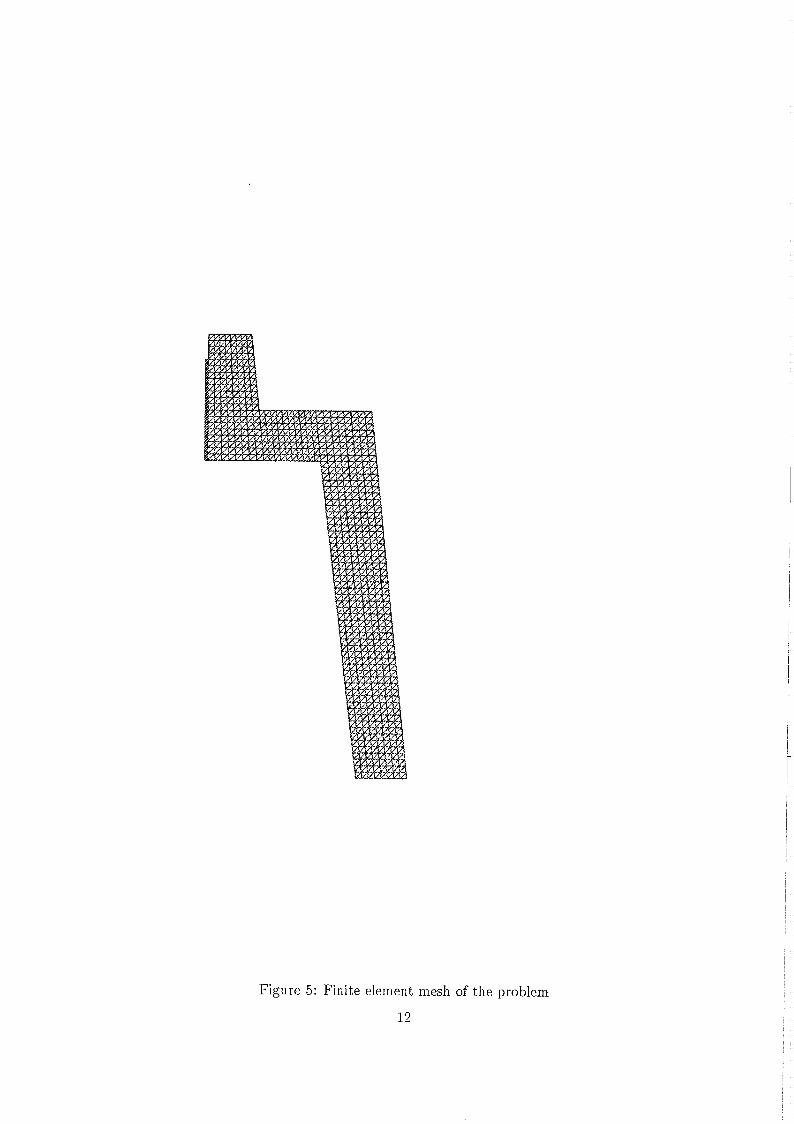
Figure 5: Finite element mesh of the problem

12

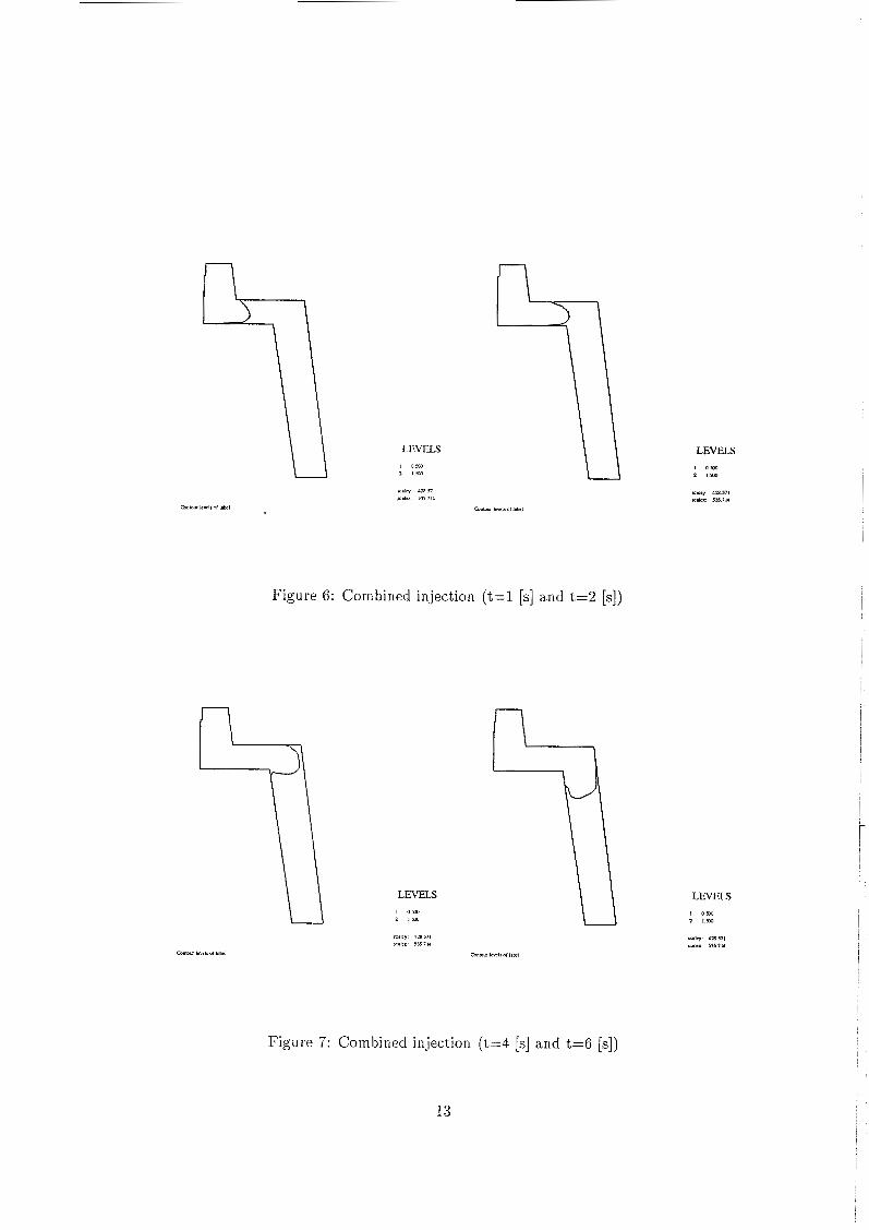
Figure 6: Combined injection (t=i [s] and t=2 [ s ] )

LEVELS

LEVELS I om 2 lm

Figure 7: Combined injection (t=4 [SI and t=6 [SI)

LEVELS I om 2 Im

i

13

LEVELS LEVELS

Figure 8: Combined injection (t=8 [s] and t=10 [SI)

LEVELS , om 2 im

Figure 9: Combined injection (t=12 [s] and t=14 [SI)

14

LEVELS

Figure 10: Sequential injection (t=l [SI and t=2 [SI)

LEVELS , 0 % 2 im

LEVELS

LEVELS

I

Figure 11: Sequential injection (t=4 [SI and t=6 [SI)

15

LEVELS

Figure 12: Sequential injection (t=8 [SI and t=10 [SI)

LEVELS I om 2 lm

Figure 13: Sequential injection ( t= i2 [SI and t=14 [SI)

16

LEVELS

Appendix A Volume of the product

radius [mm] 13.00 16.05

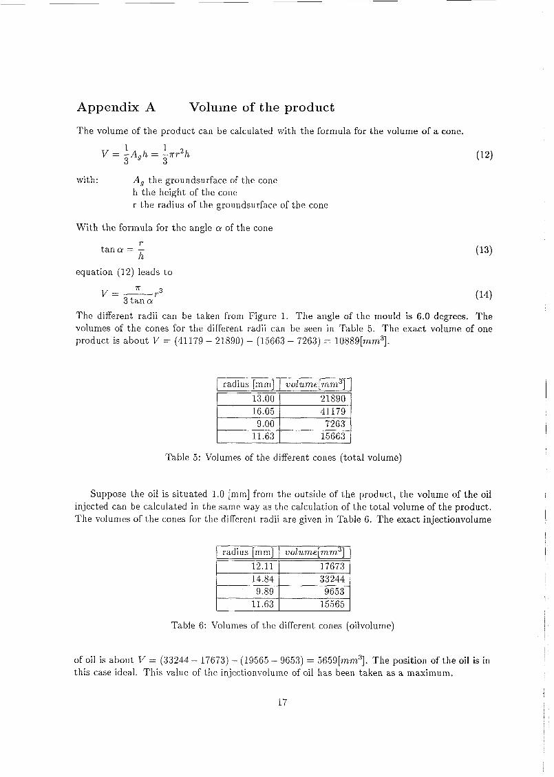
The volume of the product can be calculated with the formula for the volume of a cone.

voZume[mm3] 21890 41179

with : As the gïoündsurface of the cone h the height of the cone r the radius of the groundsurface of the cone

9.00 11.63

With the formula for the angle a of the cone r

tancu= - h

7263 15663

equation (12) leads to r v=- r3

3 t a n a

radius [min] 12.11 14.84 9.89

11.63

The different radii can be taken from Figure 1. The angle of the mould is 6.0 degrees. The volumes of the cones for the different radii can be seen in Table 5. The exact volume of one product is about V = (41179 - 21S90) - (15663 - 7263) = 10889[mm3].

volz~me[mm~] 17673 33244 9653

15565

Table 5: Volumes of the different cones (total volume)

Suppose the oil is situated 1.0 [mm] from the outside of the product, the volume of the oil injected can be calculated in the same way as the calculation of the total volume of the product. The volumes of the cones for the different radii are given in Table 6. The exact injectionvolume

of oil is about V = (33244 - 17673) - (19565 - 9653) = 5659[mm3]. The position of the oil is in this case ideal. This value of the injectionvolume of oil has been taken as a maximum.

17

I

Appendix B Listiiigs

B.l Main prograin

C

C

C

C

C

C

C

C

C

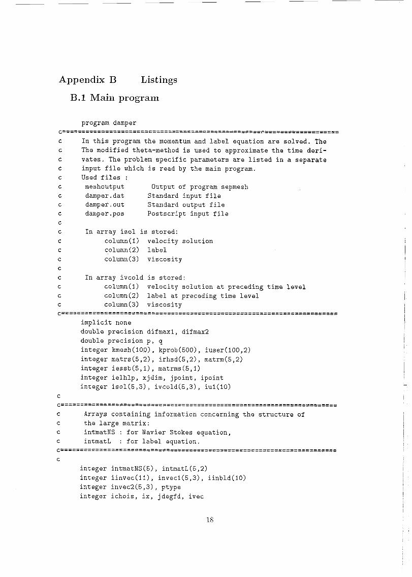
C

I n t h i s program t h e momentum and l a b e l equa t ion are so lved . The The modified theta-method i s used t o approximate t h e t ime d e r i - v a t e s . The problem s p e c i f i c parameters are l i s t e d i n a s e p a r a t e inpu t f i l e which i s read by t h e main program. Used f i l e s :

meshoutput Output of program sepmesh damper. d a t Standard inpu t f i l e damper. o u t Standard output f i l e damper .pos P o s t s c r i p t i npu t f i l e

C I n a r r a y is01 is s t o r e d : column(1) v e l o c i t y s o l u t i o n column(2) l a b e l column ( 3 ) v is cos it y

C I n array i v c o l d is s t o r e d : C coiumn(1) v e l o c i t y s o l u t i o n a t p reced ing time l e v e l C column(2) l a b e l at preceding t ime l e v e l C column ( 3 ) v i s cos it y . . . . . . . . . . . . . . . . . . . . . . . . . . . . . . . . . . . . . . . . . . . . . . . . . . . . . . . . . . . . . . . . . . . . . . . .

i m p l i c i t none double p r e c i s i o n difmaxl , difmax2 double p r e c i s i o n p , q i n t e g e r kmesh(1001, kprob(500), i u se r (100 ,2 ) i n t e g e r m a t r s ( 5 , 2 ) , i r h s d ( 5 , 2 ) , matrm(5,2) i n t e g e r i e s s b ( 5 , 1 ) , matrms(5,l) i n t e g e r i e l h l p , xjdim, j p o i n t , i p o i n t i n t e g e r i s o 1 ( 5 , 3 ) , i v c o l d ( 5 , 3 ) , i u l ( l 0 )

C

C Arrays c o n t a i n i n g information concerning t h e s t r u c t u r e of C t h e l a r g e ma t r ix : C intmatNS : f o r Navier Stokes equat ion, C i n t m a t l : f o r l a b e l equat ion.

C

i n t e g e r intmatNS(51, intmatL(5,a) i n t e g e r i i n v e c ( l i ) , i n v e c i ( 5 , 3 ) , i i n b l d ( l 0 ) i n t e g e r i n v e c 2 ( 5 , 3 ) , ptype i n t e g e r i c h o i s , i x , j deg fd , i v e c

i n t e g e r i n t ege r i n t e g e r i n t e g e r i n t e g e r i n t e g e r i n t e g e r i n t ege r i n t e g e r i n t ege r

i s t e p i , i r e s u l ( 5 , l ) , i h e l p ( 5 , 3 ) , i he lpp (5 ,3) i h l p ( 5 , 3 ) , i t e s t ( 5 , 3 ) , ibound(5,3) s h e a r v ( 5 ) , shearn(51 , i i n d e r ( 2 ) i e t a ( 5 1 , idum(5) it emp (5) j b u f f r , j b f r e e i i n p u t (500) imovestep, istep-pw i c h c r v , i s t a r t , i r o t a t , i o u t p , i t i m e

double p r e c i s i o n u s e r ( l 0 0 , 2 ) , u1(10) , a lpha2 , be t a2 double p r e c i s i o n r i n v e c ( l 1 ) double p r e c i s i o n rdum

common i b u f f r ( 2 0 O00 000) i n t ege r ibuf f r common / c b u f f r / n b u f f r , k b u f f r , i n t l e n , i b f r e e i n t e g e r n b u f f r , k b u f f r , i n t l e n , i b f r e e common /cmcdpi/ i r e f w r , i r e f r e , i r e f e r i n t e g e r i r e f w r , i r e f r e , i r e f e r common /ct ima/ t h e t a , d e l t a t , t , ra t ime(71 ,

i n t e g e r i c t i m e , n s t e p , i r t i m e double p r e c i s i o n t h e t a , d e l t a t , t , ra t ime , t s t e p common / ca r r ay / i i n f o r , in for (3 ,1500) i n t e g e r i i n f o r , i n f o r common /dprotim/ t r b , t r e , t o b , t o e , i n j e c double p r e c i s i o n t r b , t r e , t o b , t o e , i n j e c

n s t e p , i r t i m e ( 9 )

C

I

C

kmesh(1) = 100

19

r

20

C

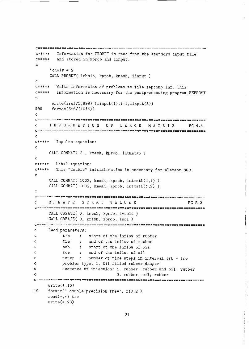
c***** Impulse equation: C

CALL COMMAT( 2 , kmesh, kprob, intmatNS ) C

c***** Label equation: c***** This “double“ initialization is necessary C

for element 800.

CALL COMMAT( 1002, kmesh, kprob, intmatL(1,l) ) CALL COMMAT( 1002, kmesh, kprob, intmatL(l,2) )

21

II II II II

II II II II II II II It II II II II II II II I1 II II II II II II II II II II II II II

II II II II II II II II II II II II II II II It II II It

n

01

O

Vi

7-í

..

n

01 -.

II II II II II

II II li II II I1 II II It II II It I1 II II II II II II II II II II II II II I1 I1

6% II

a, I1

4.J II

rn II II II II II II II II II II II II II U

O

ri

.. a, rl

-4

V

i

P

? a

u

Vi

.. II a, O

c,

s .rl m

*rl V

a, k

a

a, r

l

P

a

g .. W

.. n

k

c,

k

a, c, %

i ld

.. P

k

c, k

a, c, 'H

ld

.. P

k

P

II II II II II LI II II II I1 II II II II II II II II II I1 II It II II II It II II II II II II II li II

I1

o n

LD .rl .. ..

d

U

U

a, a

r7

d

.rl

a

a, c, rn 6,

z

O

H

b

4

p: w

b

H

a, k

O

c, 5 O O

c,

a, 5

o P

k

c, .. .. P

k

P

n

* k

3

<+i a, k

.rl

a, c, -rl k

3

.. W

a, k

'r: .. .. a, k

9

n

* k

3

Vi a, k

-rl

a, c.' .rl k

3

- .. W

P

O

c,

al O

c.', .. .. a, O

c,

n

* k

3

Vi a, k

.rl

a, c, .rl k

3

.. W

'H

a, P

II u a,

.. .. d

c, al F: c,

* k

3

Vi

a, k

*rl

a, c, .rl k

3

.. A

W

.. .. u a

6% a, c,

\ :

.rl rn .rl U

a, k

a

II e, a,

UI

c, m

e

.. .. e rl ld al a

h

rl

o 5 u

.. .. P

O

c, .. - * k

3

w a,

k

.rl

a, c, -d

k

3

v

a d d

m

a, ?

rl ld + c, F: a, k

k

u a, c, -4

k

5

* * Y

* * u

uv

'r7

F: 3 a I

c, m

.rl

A

3

* * a d a, k .L

W

a, k

O

u-( a, P

n

P

k

c, I a, k

c,

II

W

k

au

b

na

,

.. n

* k

3

y-i a, k

-4

a, c, *rl k

3

W

a, n

* k

3

V

i a, k

a, c, *rl k

3

W

rl

P

a g o c,

a, O

c,

n

O

m

n

O

m

n

O

W

m

2 c, rn

,.G

c, .rl 3

n

O

A

* * a d a,

k

W

n

* * a d a, k

W

O

a

n

-Y

U

..

5 k

M

O

W

* al c, -4

k

3

W

* a, c, .rl k

5

W

.. * W

a, c, .li

k

5

.. * W

a, c, .rl k

5 ..

O a

O

II P

k

c,

d

II a, a

O a

O

c, d

O

+I

k c,

k O

y-i

2 tJ

a

rd E

a

I4 (d

Oa,

+i

k

'5

E

a

kl

d

oa,

Vi

k

+J

k

O

Vi

2 c, ld I-, rl a, a

O

O

LD

s .rl b

* * * * * u

GI a * * Y

* * u

v0

II

c, O a

* * * * Y

u

Y

* * Y

* V

II II II U

O

o)

O

m o

d* O

u)

O

W

u

V

V

u V

I

23

CALL MAVER( matrm(l,2), ivcold(l,2), iresul(l,I), & intmatL(l,l), kprob, 5 )

I

1

24

CALL BUILD(iinbld, matrs(l,l), intmatNS, kmesh, kprob, & irhsd(l,l), matrm(l,l), isol(l,l), ivcold, & iuser(i,i), user(i,l))

iinvec(1) = 5 iinvec(2) = 32 iinvec(3) = O iinvec(4) = 0 iinvec(5) = i rinvec(1) = 3d0 CALL MANVEC( iinvec, rinvec, itest(l,l), idum, itest(l,l),

& kmesh, kprob)

C CALL PRINOV(ibound(l,l), kmesh, kprob, 2, 'bound', rdum, idum) C CALL PRINOV(itest(l,l), kmesh, kprob, 2, 'test', rdum, idum)

C array kmeshm t o workspace C

C

CALL IN1070 (kmesh(27)

25

C

C create start vector L

ichois = O ichcrv = 1001 iui(1) = 0 üi(i) = ÛdO CALL CREAVC(ichois, ichcrv, idum, ihlp(l,l), kmesh, kprob,

& iul, UI, idum, rdum) C

C define pointer in ibuffr C

CALL BOUNCD(kprob, itest, ibound, isol, & ibuffr(infor(l,kmesh(27))), ihlp)

C

C

CALL PRINOV(ihlp, kmesh, kprob, 2, >ihlp>, rdum, idum)

iinder(1) = 2 iinder(2) = 4 CALL DERIV(iinder, ihlp(l,l), kmesh, kprob, ihlp(l,i),

& iuser(I, i), user(1, i))

CALL PRINOV(ihlp, kmesh, kprob, 2, ’ ihlp’ , rdum, idum)

CALL BOUNCDl(kprob, itest, ibound, isol, & ibuffr(infor(l,kmesh(27))), ihlp)

C CALL PRINOV(isol(l,l), kmesh, kprob, 2, ’boundl’, rdum, idum)

CALL MAVER(matrs(l,l), isol, ihelpp(l,l), intmatNS, kprob, 6 )

I-

CALL SOLVE( 1, matrs(l,l), isol(l,i), irhsd(l,l), intmatNS, 85 kprob 1

CALL DIFFVC( O, isol(l,l), ivcold(l,l), kprob, difmaxl ) write(6,2000) istep,difmaxl

C

if ( ptype.eq.1) then rinvec(1) = id0

endif

CALL MANVEC( iinvec, rinvec, isol(l,2), invec2, & ieta, kmesh, kprob

CALL INI056(ivcold(l,3), 'Main')

CALL DERIV( iinder, ivcold(l,3), kmesh, kprob, iets, k iuser, user 1

iinvec(1) = 11 iinvec(2) = 32 iinvec(3) = O iinvec(4) = 1 iinvec(5) = 1

I 1

27

iinvec(6) = 3 iinvec(7) = 0 iinvec(8) = 1 iinvec(9) = 2 iinvec(í0) = 3 iinvec(l1) = 2

L

write(6,2500) t

28

2000 format( istep: ',i5,> difmaxl = >,e10.3 ) 2100 format( ' istep: >,i5,' difmax2 = >,e10.3 ) 2500 format( time= ',e10.3 ) 26'20 format( : i= ;,i3,> iuser: ',ilO,> user: ',e10.3 )

end

clearpage

C%%%%%%%%%%%%%%%%%%%%%%%%%%%%%%%%%%%%%%%%%%%%%%%%%%%%%%%%%%~%%%~~~~~~~~~

C%%%%%%%%%%%%%%%%%%%%%%%%%%%%%%%%%%%%%%%%%%%%%%%%%%%%%%%%%%%%%%%%~%%%~~%

C S U B R O U T I N E S

S U B R O U T I N E FUNVEC( rinvec, reavec, nvec, coor, outvec ) implicit none common /cmcdpi/ irefwr , iref re, iref er integer irefwr, irefre, irefer integer nvec double precision rinvec(*) , reavec(nvec) , coor(*), outvec

if (reavec(l).le.0.5dO) then

else outvec = 1.0d-1

if (reavec(l).le.1.5dO) then

else

endif

outvec = 1.0d4

outvec = 1 . 0 d 2

endif

else if (rinvec(1) .eq.2d0) then c***********************************************************************

C reavec(í)=isol(l,2) (solution of the label) C******************************************************************~****

I

if (reavec(1) .lt.OdO) then outvec = OdO

29

e l s e i f ( reavec(1) . g t .2d0) t h e n

e l s e

endif

outvec = 2d0

outvec = reavec(1)

endif

e l s e if ( r invec (1 ) .eq.3d0) t h e n c*********************************************************************** C r e a v e c ( l ) = i t e s t ( l , l ) ( = i s o l ( l , 2 ) ) . . . . . . . . . . . . . . . . . . . . . . . . . . . . . . . . . . . . . . . . . . . . . . . . . . . . . . . . . . . . . . . . . . . . . . . .

i f ( reavec (1) . It . O . 5d0) then

e l s e

endif

outvec = Id0

outvec = OdO

endif end

C

C

C

FUNCTION FUNCBC( i c h o i s , x, y, z )

i m p l i c i t none

double p r e c i s i o n t h e t a , d e l t a t , t , ra t ime i n t e g e r n c t e p , i r t i m e common /ctima/ t h e t a , d e l t a t , t , ra t ime(71 ,

double p r e c i s i o n t r b , t r e , t o b , t o e , i n j e c common /dprotim/ t r b , t r e , t o b , t o e , i n j e c double p r e c i s i o n x, y , z double p r e c i s i o n p i , ugemr, ugemo, funcbc, l a b e l double p r e c i s i o n f l o o , f l o r , a l p h a i n t e g e r i c h o i s

n s t e p , i r t i m e ( 9 )

p i = 4dO*atan(ldO) î100 = 3.5d-7 a l p h a = (6 .0 * p i ) /180

C

c**** d e f i n i t i o n of t h e inflow . . . . . . . . . . . . . . . . . . . . . . . . . . . . . . . . . . . . . . . . . C

i f ( i n j e c . eq .I) t hen f l o r = 4.25d-7

30

if (t. It. tob. or. t. gt .toe) then ugemo=OdO ugemr=f lor/ ((pi* (3.551d-3) **2) -(pi* ( O , 25d-3)**2) )

ugemo=f l oo / (pi* (O .25d-3) **2) ugemr=flor/((pi*(3.55ld-3)**2)-(pi*(O.25d-3)**2))

else

enaif endif

if (inj ec . eq. 2) then flor = 8.5d-7 if (t.lt.tob.or.t.gt.toe) then

ugemo=OdO ugemr=flor/((pi*(3.55ld-3)**2)-(pi*(O.25d-3)**2))

ugemo=floo/ (pi* ( O . 25d-3) **2) ugemr=OdO

else

endif endif

c**** definition of the time-dependent label boundary condition ******** c**** of curve 10

if (t. ge. tob. and. t , le. toe) then label=:!. OdO

else label=l .OdO

endif C

c**** ichois = 1 and 2, boundary conditions of curves 2 and 3 ********** C

if (ichois.eq.1) then funcbc=flor/(pi*((l.3d-2 + (2.9d-2-y)*dtan(alpha))**2 -

& ( O . 858d-2+(2.9d-2-y)*dtan(alpha) )**2) )*dsin(alpha)* & 4. OdO endif

if (ichois.eq.2) then funcbc=-flor/(pi*((l.3d-2 + (2.9d-2-y)*dtan(alpha))**2 -

& (0.858d-2+(2.9d-2-y)*dtan(alpha))**2))*dcos(al~ha)* & 4. OdO endif

c**** ichois = 3, boundary condition of curve 4 and 5 ****************** C

C

if (ichois. eq. 3) then funcbc=flor/(2 * pi * x * 4.0d-3) *

I

31

& 2/pi * atan(l.8d3 * (x - 4.182d-3)) endif

L

c**** ichois = 4 and 5, boundary conditions of curve 6 ***************** C

if (ichois.eq.4) then

endif fur;cuc=floï/(pi*x**2j * dsin(a1phaj

if (ichois.eq.5) then

endif funcbc=-flor/(pi*x**2) * dcos(a1pha)

C

c**** ichois = 6 and 7, boundary conditions of curve 7 ******i**********

L

if (ichois.eq.6) then funcbc=flor/(pi*(2.5d-3+(4.5d-2 - y)*dtan(alpha))**2 -

& ( O . 25d-3) **2) * dsin(a1pha) endif

if (ichois . eq. 7) then funcbc=-flor/(pi*(2.5d-3+(4.5d-2 - y)*dtan(alpha))**2 -

& ( O . 25d-3) **2) * dcos (alpha) endif

L

c**** ichois = 8, boundary condition of curve 8 . . . . . . . . . . . . . . . . . . . . . . . . L,

if (ichois.eq.8) then

endif funcbc=-2d0*ugemr*(l.OdO-(~x-l.9Old-3)/(l.65ld-3))**2)

C

c**** ichois = 9, boundary condition of curve 9 . . . . . . . . . . . . . . . . . . . . . . . . C

if (ichois.eq.9) then funcbc=-flor/(pi*(2.5d-3+(4.5d-2 - y)*dtan(alpha))**2 -

& (O. 25d-3) **2) endif

L

c**** ichois = 10, boundary condition of curve 10 . . . . . . . . . . . . . . . . . . . . . . L

if (ichois.eq.10) then

endif funcbc=-2d0*ugemo*(l.OdO-(x/(O,25d-3))**2)

L

c**** ichois = li, boundary conditions of curves 13, 14 and 15 * I T * * * * * * *

I i

,

C

if (ichois.eq.11) then

32

funcbc=flor/(2*pi*4.Od-3*(x+l.Od-5)) * & 2/pi * atan(1.8d3 * x) endif

L

c**** ichois = 12 and 13, boundary condition of curve 16 *************** C

if (ichois.eq.í2j then funcbc=flor/(pi*((l.3d-2 + (2.9d-2-y)*dtan(alpha))**2 -

(O .858d-2+(2.9d-2-y) *dtan(alpha) )**2) )*dsin(alpha)* & & 2. OdO endif

if (ichois.eq. 13) then funcbc=-flor/(pi*((l.3d-2 + (2.9d-2-y)*dtan(alpha))**2 -

& ( O . 858d-2+ (2.9d-2-y) *dtan(alpha) ) **2) *dcos (alpha) * & 2. OdO endif

C c**** ichois = 14, label of curve 10 st^**+*

C

if (ichois.eq.14) then

endif end

funcbc=label

C C

C

SUBROUTINE BOUNCD( kprob, itest, ibound, & isol, kmeshm, ihlp)

C

c input/output parameters

implicit none C

C

c common blocks C

integer irefwr, irefre, irefer common /cmcdpi/ irefwr, irefre, irefer save /cmcdpi/

C

integer ibuffr common ibuffr(20 O00 000)

L

integer nbuffr, kbuffr, intlen, ibfree

33

common / c b u f f r / n b u f f r , kbuf f r , i n t l e n , i b f r e e save /cbuf f r/

i n t e g e r i i n f o r , i n f o r common / c a r r a y / i i n f o r , in for (3 ,1500) save /carray/

C

double p r e c i s i o n t h e t a , d t , t , ra t ime i n t e g e r i r t i m e , n s t e p common /ct ima/ t h e t a , d t , t , ra t ime(71 ,

save /c t ima/

double p r e c i s i o n t r b , t r e , t o b , t o e , i n j e c common /dprotim/ t r b , t r e , t o b , t o e , i n j e c

& n s t e p , i r t ime(9 )

C

C

c l o c a l v a r i a b l e s C

i n t e g e r i n o , ndegfd, j no , n , nc rv , nnocrv(100) , i , idum

c a l l e ropen(>bouncd>)

do 25 i = 1, 5 t e s t 3 ( i ) = OdO t e s t 2 ( i ) = OdO

25 cont inue

ncrv = kmeshm(2) - 6 - kmeshm(1)

do 21 n = i, ncrv C w r i t e ( i r e f w r , * ) Incrv = I , ncrv

nnocrv(n) = kmeshm(5 + n) - kmeshm(4 + n) C w r i t e ( i r e f w r , * ) >nnocrv = ’ , nnocrv(n)

21 cont inue do 31 n = 1, ncrv

i f (n.eq.8.or.n.eq.lO.or.n.eq.ll.or.n.eq.12) t h e n

e l s e d i f = OdO

i f (n .eq .1) t hen d i f = OdO

e l s e d i f = Id0

endi f endi f

34

C

C

C

C

w r i t e ( i r e f w r , * ) ’ d i f 0 =’, d i f i f ( d i f . ne . OdO) then

do 22 ino = 1 , nnocrv(n) j n o = kmeshm(kmeshm(2) + kmeshm(4+n) - 1 + i no - 1)

w r i t e ( i r e f w r , * ) ’ jnoû =’, j no ndegfd = 2 cal: ge tvec(kprob , i bound( í , i ) , j n o , bound, ndegfd) ndegfd = 1 c a l l ge tvec(kprob , i t e s t ( l , l ) , j n o , t e s t , ndegfd)

t e s t 2 ( 1 ) = bound(1) * t e s t ( 1 ) t e s t 2 ( 2 ) = bound(2) * t e s t ( 1 )

w r i t e ( i r e f w r , * ) ’ t e s t 2 ( 1 ) 0 = ’ , t e s t 2 ( i ) w r i t e ( i r e f w r , * ) ’ t e s t 2 ( 2 ) 0 = ’, t e s t 2 ( 2 )

c a l l putvec(kprob, i s o l ( l , l ) , j n o , t e s t 2 , idum) c a l l putvec(kprob, i h l p ( í , l ) , j n o , t e s t , idum)

22 cont inue endif

31 cont inue

c a l l e r c l o s (’bouncd’) end

L

C

SUBROUTINE BOUNCDl( kprob, i t e s t , ibound, & i s o l , kmeshm, i h l p )

C

c i npu t /ou tpu t parameters C

i m p l i c i t none

i n t e g e r kmeshm(*), kprob(*) , i t e s t ( 5 , * ) , i s o l ( 5 , * ) , ibound(5 ,*) , & i h l p (5 , *I

C

c common blocks C

i n t e g e r i r e f w r , i r e f r e , i r e f e r common /cmcdpi/ i r e f w r , i r e f r e , i r e f e r save /cmcdpi/

i n t ege r ibuf f r common i b u f f r ( 2 0 O00 000)

i n t e g e r n b u f f r , k b u f f r , i n t l e n , i b f r e e common / c b u f f r / n b u f f r , k b u f f r , i n t l e n , i b f r e e save /cbuf f r/

C

C

35

C

integer iinfor, infor common /carray/ iinfor, infor(3,1500) save /carray/

double precision theta, dt, t, ratime integer irtime, nstep common /ctima/ theta, dt, t, ratime(71,

save /ctima/

double precision trb, tre, tob, toe, injec common /dprotim/ trb, tre, tob, toe, injec

C

& nstep, irtime(9)

C

C

c local variables C

integer ino, ndegfd, jno, n, ncrv, nnocrv(l001, i, idum

double precision bound(51, test(5), test2(5), & dif

call eropen(’bouncd1))

do 25 i = i , 5 test2(i) = OdO

25 continue

ncrv = kmeshm(2) - 6 - kmeshm(1)

do 21 n = 1, ncrv C write(irefwr,*) ’ncrv = ’ , ncrv

nnocrvh) = kmeshm(5 + n) - kmeshm(4 + n) C write(irefws,*) ’nnocrv =I, nnocrv(n) 21 continue

do 31 n = i , ncrv if (n.eq.8.or.n.eq.lO.or.n.eq.ll.or.n.eq.12) then

else dif = OdO

if (n.eg.1) then dif = OdO

else dif = id0

endif endif

C write(irefwr,*) ’ difl =’, dif if (dif .ne. OdO) then do 22 ino = 1 , nnocrv(n) jno = kmeshm(kmeshm(2) + kmeshm(4+n) - 1 + ino - 1)

36

C

C

C

write(irefwr,*) 'jnol = ' , jno ndegfd = 2 call getvec(kprob, ibound(l,l), jno, bound, ndegfd) ndegfd = I call getvec(kprob, ihlp(l,l), jno, test, ndegfd) test2(1) = bound(1) * test(1) testS(2) = bound(2) * test(1) write(irefwr,*) 'test2(i)l = > > testS(í) write(irefwr,*) 'test2(2)1 = ', test2(2)

call putvec(kprob, isol(l,l), jno, test2, idum) 22 continue

endif 31 continue

call erclos ('bouncdl') end

c . . . . . . . . . . . . . . . . . . . . . . . . . . . . . . . . . . . . . . . . . . . . . . . . . . . . . . . . . . . . . . . . . . . . . . cdccgetvec

subroutine getvec( kprob, ivec, ino, vec, ndegfd ) c c . . . . . . . . . . . . . . . . . . . . . . . . . . . . . . . . . . . . . . . . . . . . . . . . . . . . . . . . . . . . . . . . . . . . . . C

C

C

C

C

C

C

C

C

C

C

C

C

C

C

C

C

C

C

C

C

C

C

programmer Leo Caspers version 1.1 date 03-08-94 (LC: complete revision) version 1.0 date 20-11-91

copyright (c) 1991 "VIp" permission to copy or distribute this software or documentation in hard copy or soft copy granted only by written license obtained from "VIp". all rights reserved. no part of this publication may be reproduced, stored in a retrieval system ( e.g., in memory, disk, or core) or be transmitted by any means, electronic, mechanical, photocopy, recording, or otherwise, without written permission from the publisher.

. . . . . . . . . . . . . . . . . . . . . . . . . . . . . . . . . . . . . . . . . . . . . . . . . . . . . . . . . . . . . . . . . . . . . .

Store all dofs of array is01 for nodal point ino into vec. Store # dofs into ndegfd Only allow vector types 110, 115 All dofs must be doubles Length of vec on input is stored in ndegfd

c . . . . . . . . . . . . . . . . . . . . . . . . . . . . . . . . . . . . . . . . . . . . . . . . . . . . . . . . . . . . . . . . . . . . . .

37

C

C INPUT / OUTPUT PARAMETERS

i m p l i c i t none

i n t e g e r i n o , ndegfd

i n t e g e r kprob(*) i vec (5 ) double p r e c i s i o n vec(*)

C

C kprob i s t anda rd sepran array C i vec i s t anda rd sepran array C ino i node number of which va lue i s d e s i r e d C ndegfd i / o inpu t : maximum allowed C ou tpu t : a c t u a l l eng th C vec O va lues of i v e c i n ino C

c . . . . . . . . . . . . . . . . . . . . . . . . . . . . . . . . . . . . . . . . . . . . . . . . . . . . . . . . . . . . . . . . . . . . . . C

C PARAMETERS IN COMMON BLOCKS C

i n t e g e r i b u f f r common i b u f f r ( 1 )

C

C / i b u f f r / C b lank common C

C ibuf f r (1) a r r a y f o r s t o r a g e of l a r g e i n t . and dp. a r r a y s c

i n t e g e r i i n f o r , i n f o r common / ca r r ay / i i n f o r , i n f o r ( 3 , 1 5 0 0 )

c L,

C / c a r r a y / C in format ion about i b u f f r C

C i i n f o r g i v e s number of t ypes s t o r e d i n i n f o r C i n f o r ( . . ) in format ion of arrays s t o r e d i n i b u f f r C

c . . . . . . . . . . . . . . . . . . . . . . . . . . . . . . . . . . . i n t e g e r n b u f f r , k b u f f r , i n t l e n , i b f r e e common / c b u f f r / n b u f f r , k b u f f r , i n t l e n , i b f r e e save / c b u f f r /

I

,

C /cbuf f r/ c Severa l v a r i a b l e s r e l a t e d t o t h e common b u f f e r i b u f f r

3s

L.

c n b u f f r Declared l e n g t h of array i b u f f r c kbuf f r Last p o s i t i o n used i n i b u f f r c i n t l e n C an i n t e g e r v a r i a b l e c i b f r e e Next f r e e p o s i t i o n i n a r r a y i b u f f r

Length of a r e a l v a r i a b l e d iv ided by t h e l e n g t h of

C c . . . . . . . . . . . . . . . . . . . . . . . . . . . . . . . . . . .

i n t e g e r i r e f w r , i r e f r e , i r e f e r common /cmcdpi/ i r e f w r , i r e f r e , i r e f e r

C

C /cmcdpi/ c u n i t numbers of i / o f i l e s c C i r e f w r u n i t number s t a n d a r d output C i r e f re u n i t number s t a n d a r d inpu t C i r e f e r u n i t number s t anda rd e r r o r f i l e c

c . . . . . . . . . . . . . . . . . . . . . . . . . . . . . . . . . . . . . . . . . . . . . . . . . . . . . . . . . . . . . . . . . . . . . . c C LOCAL PARAMETERS

i n t e g e r i n d p r f , indprh, indprp, nphys, i pvec , i p k p r f , ndgfdm, & ipkprh

ci

C #name # i / o #explanat ion L

c . . . . . . . . . . . . . . . . . . . . . . . . . . . . . . . . . . . . . . . . . . . . . . . . . . . . . . . . . . . . . . .

C SUBROUTINES CALLED

C EROPEN #exp lana t ion C INIO55 #explanat ion C WRVEC #explanat i o n C ERCLOS #explanat ion

c . . . . . . . . . . . . . . . . . . . . . . . . . . . . . . . . . . . . . . . . . . . . . . . . . . . . . . . . . . . . . . . . . . . . . .

C

C

C

c c a l l eropen ( ' g e t v e c > ) I

c Save max of ndegfd

ndgfdm = ndegfd

c Get p o i n t e r s of kprobf , kprobh, kprobp, is01

call ini075 ( ivec , kprob , indprf indprh, indprp, nphys)

ipkprf = max( 1, infor(1,indprf) if ( indprf .gt . O )then

else

endif

ndegfd=ibuffr(ipkprf+ino)-ibuffr(ipkprf+ino-1)

ndegf d=nphys

c Check max ndegfd

if ( ndegfd .It. O .or. ndegfd .gt. ndgfdm 1 then write(irefwr,*)'getvec: number of degrees of freedom is',

write(irefwr ,*) ' write(irefwr,*)' allowed ' , ndgfdm, ' or less than zero' call instop

& ndegf d which is greater than the maximum'

endif

if( ndegfd .eq. O )goto 1000

ipkprh = max( 1 infor(1 ,indprh) ) ipvec=inf or ( i ivec (1) 1

c Do the copying

call vputOl( ibuffr(ipvec1, ibuffr(ipkprh1, ibuffr(ipkprf), & indprh, indprf, ndegfd, ino, vec, 1 )

1000 call erclos ( 'getvec' 1

end cdc*eor

cdccputvec subroutine putvec( kprob, ivec, ino, vec, idum )

C c . . . . . . . . . . . . . . . . . . . . . . . . . . . . . . . . . . . . . . . . . . . . . . . . . . . . . . . . . . . . . . . . . . . . . . L

C programmer Leo Caspers C version 1.2 date 02-10-94 (LC: add dummy argument) C version i . 1 date 03-08-94 (LC: complete revision) C version 1.0 date 20-11-91

c copyright ( c ) 1991 "VIP" c

C

permission to copy or distribute this software or documentation

40

c c ob ta ined from " V I P " . c c s t o r e d i n a r e t r i e v a l system ( e . g . , i n memory, d i s k , o r co re> c c c p u b l i s h e r .

c . . . . . . . . . . . . . . . . . . . . . . . . . . . . . . . . . . . . . . . . . . . . . . . . . . . . . . . . . . . . . . . . . . . . . .

i n hard copy o r s o f t copy g ran ted only by w r i t t e n l i c e n s e

a l l r i g h t s r e se rved . no p a r t of t h i s p u b l i c a t i o n may be reproduced,

o r be t r a n s m i t t e d by any means, e l e c t r o n i c , mechanical , photocopy, r eco rd ing , o r o the rwise , without w r i t t e n permiss ion from t h e

C

C

C

C Only a l low v e c t o r t ypes 110, 115 C All dofs must be doubles

c . . . . . . . . . . . . . . . . . . . . . . . . . . . . . . . . . . . . . . . . . . . . . . . . . . . . . . . . . . . . . . . . . . . . . .

C INPUT / OUTPUT PARAMETERS

S t o r e a l l do f s of array is01 f o r nodal p o i n t ino i n t o vec.

C

C

i m p l i c i t none

i n t e g e r i n o , idum

i n t e g e r kprob(*) , ivec(5) double p r e c i s i o n vec(*)

C

C kprob i s t anda rd sepran array C i v e c i s t anda rd sepran array C ino i node number of which va lue i s d e s i r e d C vec O va lues of i vec i n ino C i dum i dummy f o r h i s t o r i c a l reasons

c . . . . . . . . . . . . . . . . . . . . . . . . . . . . . . . . . . . . . . . . . . . . . . . . . . . . . . . . . . . . . . . . . . . . . .

C PARAMETERS IN COMMON BLOCKS

C

C

C

i n t ege r ibuf f r common i b u f f r ( 1 )

C

C / i b u f f r / C b lank common

C ibuf f r (I) C

a r r a y f o r s t o r a g e of l a r g e i n t . and dp. a r r a y s

i n t e g e r i i n f o r , i n f o r common / c a r r a y / i i n f o r , i n f o r ( 3 , i 5 0 0 )

41

C

C / c a r r a y / C information about i b u f f r

C i i n f o r g i v e s number of t ypes s t o r e d i n i n f o r C i n f o r ( . .> information of a r r a y s s t o r e d i n i b u f f r

C

C e - _ - - - - - - - - - - - - - - - - - - _ _ _ _ _ _ _ _ D _ _ _ _ _ _

i n t e g e r n b u f f r , k b u f f r , i n t l e n , i b f r e e common / c b u f f r / n b u f f r , k b u f f r , i n t l e n , i b f r e e save / c b u f f r /

C /cbuf f r/ c S e v e r a l v a r i a b l e s r e l a t e d t o t h e common b u f f e r i b u f f r C

c n b u f f r Declared l e n g t h of array i b u f f r c kbuf f r Last p o s i t i o n used i n i b u f f r c i n t l e n C an i n t e g e r v a r i a b l e c i b f r e e Next f r e e p o s i t i o n i n a r r a y i b u f f r

Length of a r e a l v a r i a b l e d iv ided by t h e l e n g t h of

L

c - . . . . . . . . . . . . . . . . . . . . . . . . . . . . . . . . . . i n t e g e r i r e f w r , i r e f r e , i r e f e r common /cmcdpi/ i r e f w r , i r e f r e , i r e f e r

/ cmcdp i/ u n i t numbers of i / o f i l e s

i r e f w r u n i t number s t anda rd output i r e f r e i r e f e r u n i t number s t anda rd e r r o r f i l e

u n i t number s t anda rd inpu t

L

c . . . . . . . . . . . . . . . . . . . . . . . . . . . . . . . . . . . c . . . . . . . . . . . . . . . . . . . . . . . . . . . . . . . . . . . . . . . . . . . . . . . . . . . . . . . . . . . . . . . . . . . . . . i.

C LOCAL PARAMETERS

i n t e g e r i n d p r f , i ndprh , i ndprp , nphys, i pvec , i p k p r f , & ipkprh, ndegf d

C

C #name # i / o #exp lana t ion

c . . . . . . . . . . . . . . . . . . . . . . . . . . . . . . . . . . . . . . . . . . . . . . . . . . . . . . . . . . . . . . . . . . . . . .

C SUBROUTINES CALLED

C

C

C

42

C EROPEN #explanation C IN1075 #explanation C ERCLOS #explanation

c . . . . . . . . . . . . . . . . . . . . . . . . . . . . . . . . . . . . . . . . . . . . . . . . . . . . . . . . . . . . . . . . . . . . . . C

L

cali eropen ( >putvec' )

c Get pointers of kprobf, kprobh, kprobp, is01

call ini075( ivec, kprob, indprf, indprh, indprp, nphys)

ipkprf = max( 1, infor(1,indprf) ) if ( indprf .gt . O )then

else

endif

ndegfd=ibuffr(ipkprf+ino)-ibuffr(ipkprf+ino-i)

ndegfd=nphys

if( ndegfd .eq. O )goto 1000

ipkprh = max( 1, infor(1, indprh) ) ipvec=infor(i ,ivec(i>>

c Do the copying

call vputOl( ibuffr(ipvec1, ibuffr(ipkprh1, ibuffr(ipkprf) , & indprh, indprf, ndegfd, ino, vec, 2 )

1000 call erclos ( >putvec' )

end cdc*eor

cdccvput01 subroutine vputOl( vector, kprobh, kprobf, indprh, indprf,

& ndegfd, ino, vecusr, ichois ) c . . . . . . . . . . . . . . . . . . . . . . . . . . . . . . . . . . . . . . . . . . . . . . . . . . . . . . . . . . . . . . . . . . . . . .

C

C programmer Leo Caspers C version 1.0 date 23-06-94 (First draft)

c copyright (c) 1993 "Vip" c permission to copy or distribute this software or documentation c c obtained from "VIP". c

C

in hard copy or soft copy granted only by written license

all rights reserved. no part of this publication may be reproduced,

43

c s t o r e d i n a r e t r i e v a l system ( e . g . , i n memory, d i s k , o r c o r e ) c o r be t r a n s m i t t e d by any means, e l e c t r o n i c , mechanical, photocopy, c r eco rd ing , o r o the rwise , without w r i t t e n permission from t h e c p u b l i s h e r . C

c . . . . . . . . . . . . . . . . . . . . . . . . . . . . . . . . . . . . . . . . . . . . . . . . . . . . . . . . . . . . . . . . . . . . . . C

C DESCRIPTION C

C # e x p l a i n sub rou t ine

c . . . . . . . . . . . . . . . . . . . . . . . . . . . . . . . . . . . . . . . . . . . . . . . . . . . . . . . . . . . . . . . . . . . . . . C

C KEYWORDS C

c . . . . . . . . . . . . . . . . . . . . . . . . . . . . . . . . . . . . . . . . . . . . . . . . . . . . . . . . . . . . . . . . . . . . . . c.

c INPUT / OUTPUT PARAMETERS L

i m p l i c i t none i n t e g e r ndegfd, i n o , indprh, i n d p r f , i c h o i s i n t e g e r kp robf (* ) , kprobh(*) double p r e c i s i o n v e c t o r ( * ) , vecusr(*)

C

c i c h o i s i 1: c a l l e d by ge tvec : copy v e c t o r t o vecus r C 2: c a l l e d by putvec: copy vecusr t o v e c t o r r L

c . . . . . . . . . . . . . . . . . . . . . . . . . . . . . . . . . . . . . . . . . . . . . . . . . . . . . . . . . . . . . . . . . . . . . . . . C

C u COMMON BLOCKS - C

c . . . . . . . . . . . . . . . . . . . . . . . . . . . . . . . . . . . . . . . . . . . . . . . . . . . . . . . . . . . . . . . . . . . . . . C

C LOCAL PARAMETERS C

i n t e g e r i u n d e r , i C

C iunder i r e l a t i v e p o i n t e r t o 1st dof of node ino c . . . . . . . . . . . . . . . . . . . . . . . . . . . . . . . . . . . . . . . . . . . . . . . . . . . . . . . . . . . . . . . . . . . . . . L

C SUBROUTINES CALLED

C

C EROPEN: Produces concatenated name of l o c a l sub rou t ine C ERRSUB: Er ro r messages

ERCLOS: Resets o l d name of p rev ious sub rou t ine of h i g h e r l e v e l

C

44

c . . . . . . . . . . . . . . . . . . . . . . . . . . . . . . . . . . . . . . . . . . . . . . . . . . . . . . . . . . . . . . . . . . . . . . C

C I/O c none c . . . . . . . . . . . . . . . . . . . . . . . . . . . . . . . . . . . . . . . . . . . . . . . . . . . . . . . . . . . . . . . . . . . . . . C

C ERROR MESSAGES c - c . . . . . . . . . . . . . . . . . . . . . . . . . . . . . . . . . . . . . . . . . . . . . . . . . . . . . . . . . . . . . . . . . . . . . . C

C PSEUDO CODE

c trivial C

...................................................................... ...................................................................... C

call eropen ( 'vputOíJ )

if ( indprf .gt . O )then

else

endif

iunder = kprobf(ino)+l

iunder = (ino- 1) *ndegf d+ 1

1

if( ichois .eq. 1 )then

c Called by getvec

if( indprh .eq. O )then do 10 i = 1, ndegfd

vecusr(i) = vector(iunder+i-1) 10 continue

else do 20 i = 1, ndegfd

vecusr(i) = vector(kprobh(iunder+i-1)) 20 continue

endif else

c Called by putvec

if( indprh .eq. O )then do 30 i = 1, ndegfd

vector(iunder+i-1) = vecusr(i) 30 continue

else do 40 i = 1, ndegfd

vector(kprobh(iunder+i-I)) = vecusr(i)

i

45

40 cont inue endif

endif

c a l l e r c l o s ( 'vputOí ' ) end

cdc*eor

46

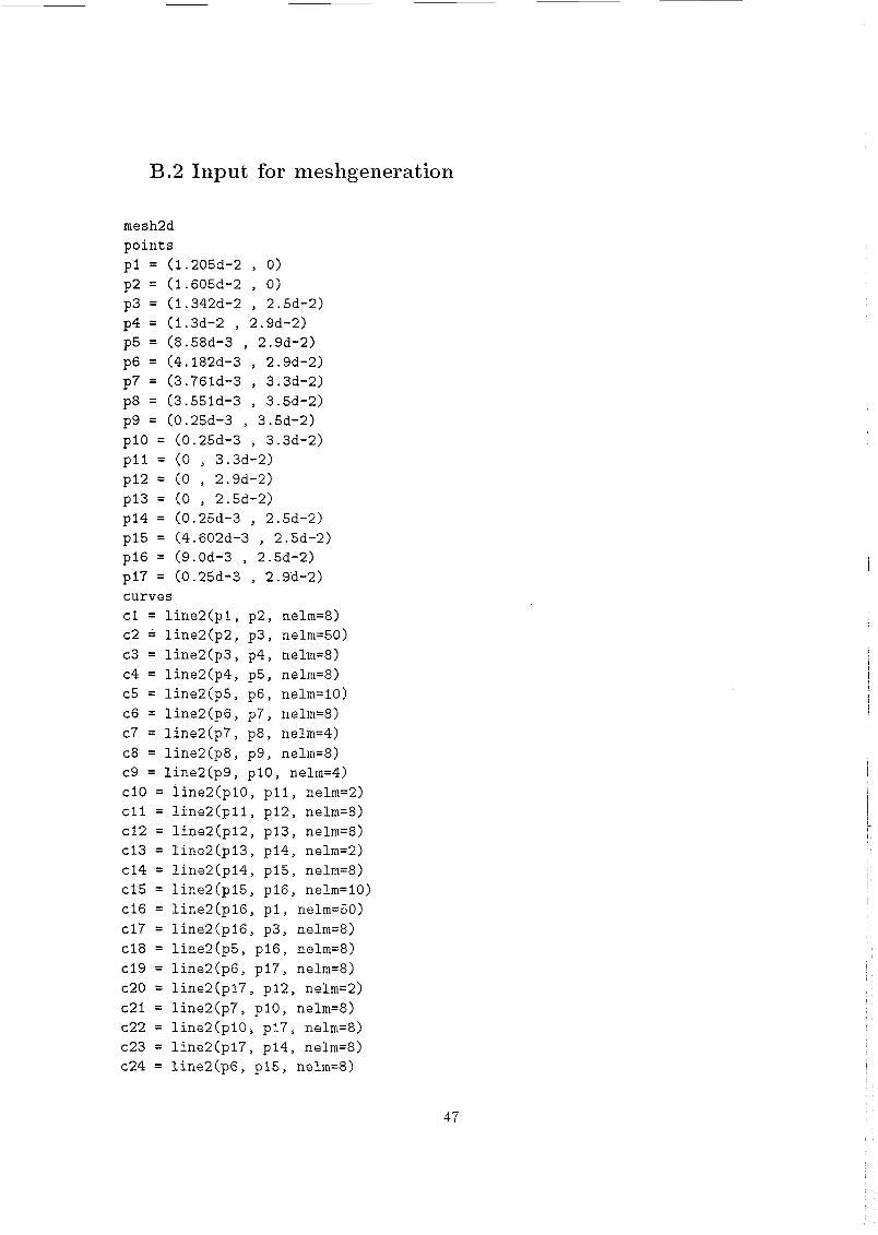
B.2 Input for meshgeneration

mesh2d p o i n t s p l = (1.205d-2 , O ) p2 = (1.605d-2 , O > p3 = (1.342d-2 , 2.5d-2) p4 = (1.3d-2 , 2.9d-2) p5 = (8.58d-3 , 2.9d-2) p6 = (4.182d-3 , 2.9d-2) p7 = (3.761d-3 , 3.3d-2) p8 = (3.551d-3 , 3.5d-2) p9 = (0.25d-3 , 3.5d-2) p i 0 = (0.25d-3 , 3.3d-2) p l l = ( O 3.3d-2) p i 2 = ( O , 2.9d-2) p13 = ( O , 2.5d-2) p14 = (0.25d-3 , 2.5d-2) p i 5 = (4.602d-3 , 2.5d-2) p16 = (9.0d-3 , 2.5d-2) p17 = (0.25d-3 , 2.9d-2) curves c l = l i n e 2 ( p l , p2, nelm=8) c2 = l i n e 2 ( p 2 , p3, nelm=50) c3 = l i n e 2 ( p 3 , p4, nelm=8) c4 = l i n e 2 ( p 4 , p5, nelm=8) c5 = l i n e 2 ( p 5 , p6, nelm=lO) c6 = l i n e 2 ( p 6 , p7, nelm=8) c7 = l i n e 2 ( p 7 , p8 , nelm=4) c8 = l i n e 2 ( p 8 , p9, nelm=8) c9 = l i n e 2 ( p 9 , p10, nelm=4) c î û = l i n e 2 ( p l 0 , pil, nelm=2) c l l = l i n e 2 ( p i l , p12, nelm=8) c12 = l ine2(p12, p13, nelm=8) c13 = l ine2(p13, p14, nelm=2) c14 = l ine2(p14, p15, nelm=8) c15 = l ine2(p15, p16, nelm=lO) c16 = l ine2(p16, p l y nelm=50) c17 = l i n e 2 ( p l 6 , p3, nelm=8) c18 = l i n e 2 ( p 5 , p16, nelm=8) c19 = l i n e 2 ( p 6 , p17, nelm=8) c2O = l i n e 2 ( p 1 7 , p12, nelm=2) c21 = l i n e 2 ( p 7 , p10, nelm=8) c22 = l i n e 2 ( p l 0 , p17, nelm=8) c23 = l ine2(p17, p14, nelm=8) c24 = l i n e 2 ( p 6 , p15, nelm=8)

47

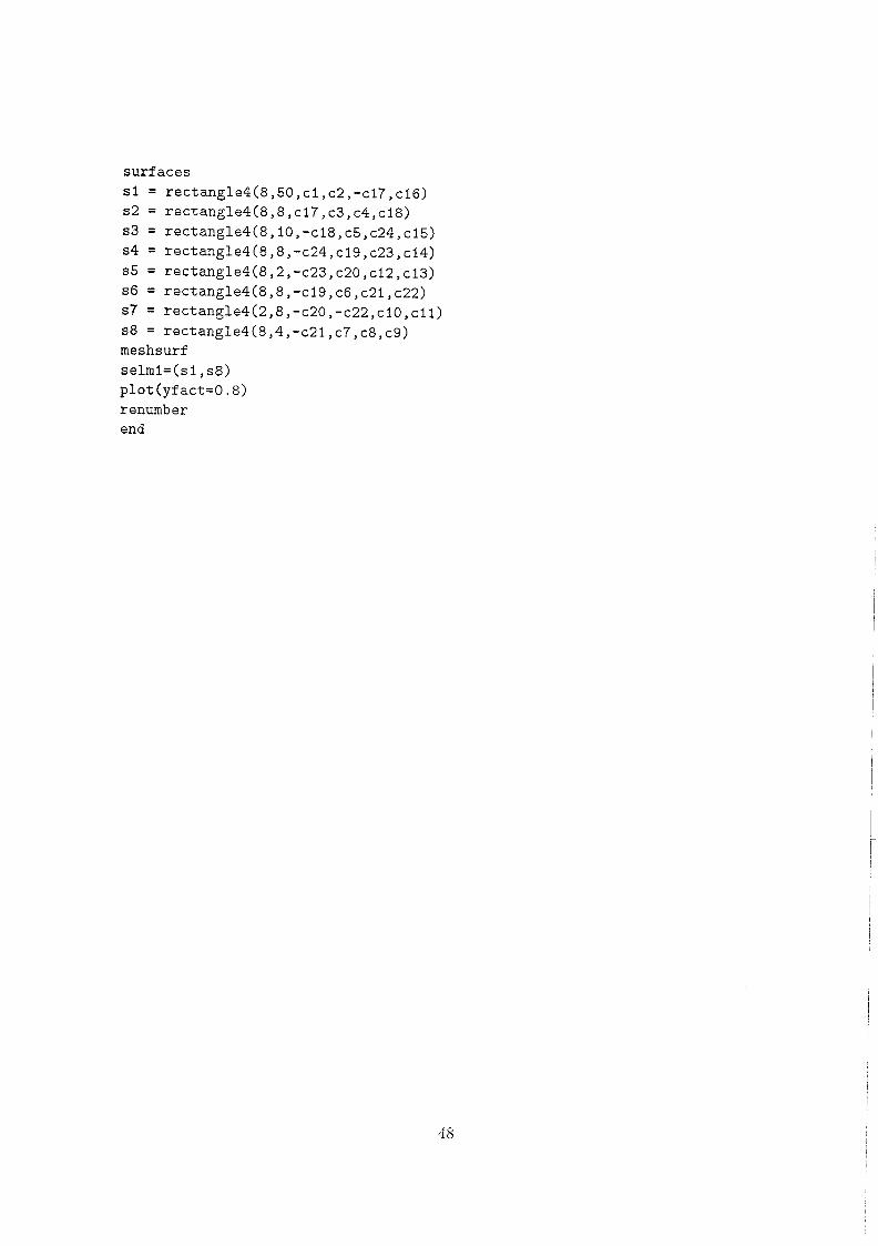
surf aces SI = rectangle4(8,50,cl,c2,-c17,cl6) s2 = rectangle4(8,8,c17,c3,c4,cl8) s3 = rectangle4(8,10 ,-c18, c5,c24, c15) s4 = rectangle4(8,8,-c24,c19,c23,~14~ s5 = rectangle4(8,2,-c23,c2O,c12,~13) s6 = rectangle4(8,8,-cl9,c6,c2l,c22) s7 = rectangle4(2,8,-c20,-c22,clO,cll~ s8 = rectangle4(8,4,-~21,~7,~8,~9) mes hsurf selml=(sl ,s8) plot(yfact=0.8) renumb er end

48

B.3 Iiiput for the solver

# Type number for Navier Stokes

# Type number for label

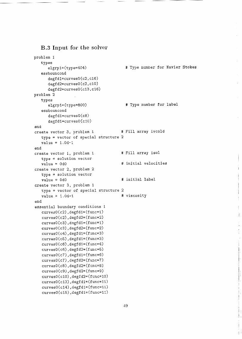
problem 1 types

eïgrpl= (type=404)

degfdl=curvesO(c2,ci5? degfd2=curvesO(c2,ciO) degfd2=curves0(cl3,cl6)

essbouncond

problem 2 types

essbouncond elgrpl= (type=800)

degfdl=curvesO(c8) degf d 1 =curves0 (c 1 O )

end create vector 3, problem 1 # Fill array ivcold

type = vector of special structure 2 value = 1 .Od-1

end create vector i, problem I # Fill array is01

type = solution vector value = OdO # initial velocities

type = solution vector value = OdO # initial label

type = vector of special structure 2 value = 1 .Od-I # viscosity

create vector 2, problem 2

create vector 3, problem 1

end essential boundary conditions 1

curvesO(c2), degf dl=(func=l) curves0 (c2) , degf d2= (func=2) curvesO(c3) ,degfdi=(func=l) curves0 (c3) , degf d2= (func=2) curves0 (c4) , degf d l = (func=3) curvesO(c5) ,degfdl=(func=3) curves0(c6),degfdl=(func=4) curves0(c6),degfd2=(func=5) curvesO(c7) ,degfdl=(func=5) curves0(c7),degfd2=(func=7) curvesO(c8) ,degfd2=(func=8) curves0(c9),degfd2=(func=9) curvesO(c10) ,degfd2=(func=iO) curvesO(cl3) ,degf dl=(func=ll) curves0 (c14) , degf di= (func=ll) curves0 (c15) , degf di= (func=ll)

49

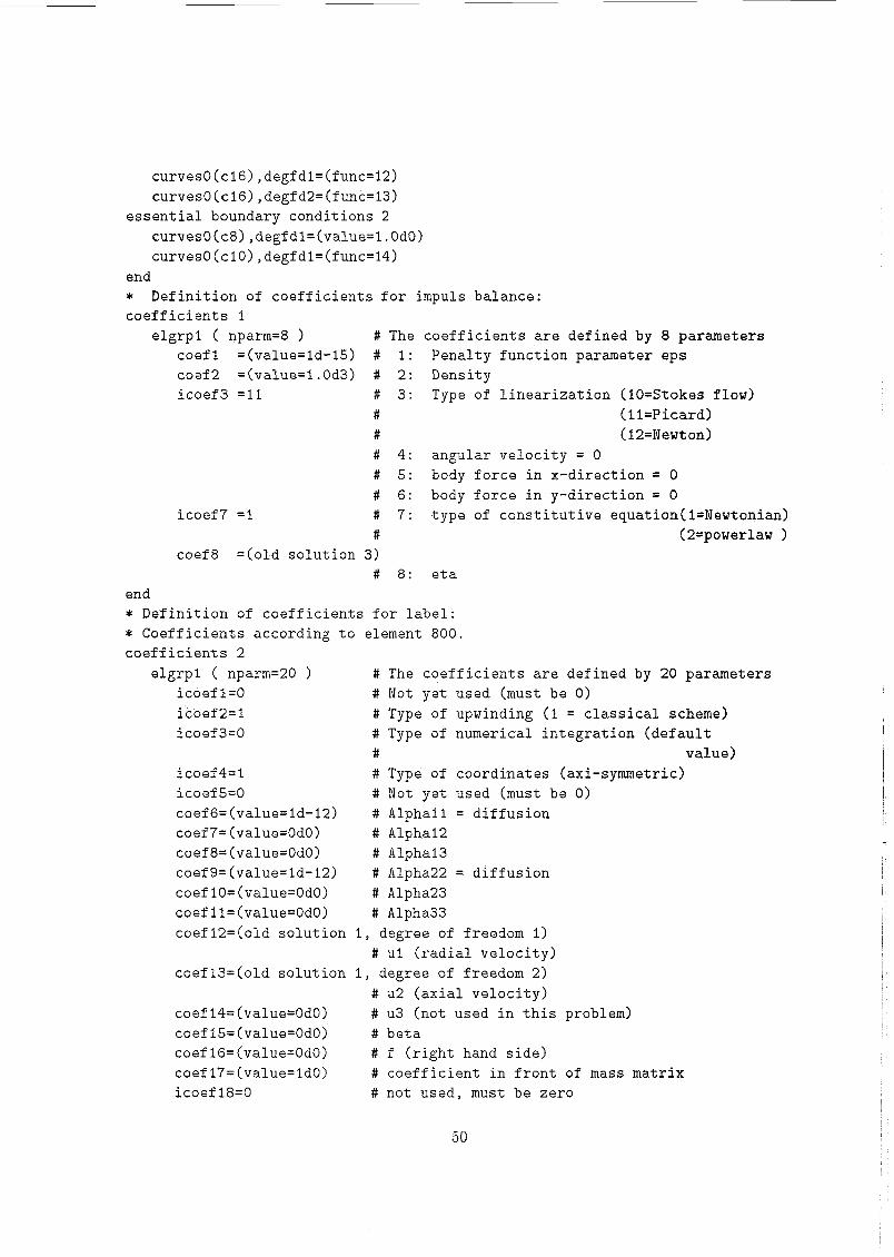
curvesO(cl6) ,degfdl=(func=l2) curves0 (c16) , degf d2=(func=13)

curvesO(c8) ,degfdl=(value=l .OdO) curvesO(clO),degfdl=(func=14)

essential boundary conditions 2

end * Definition of coefficients for impuls balance: coefficients i

elgrpl ( nparm=8 # The coefficients are defined by 8 parameters coefl =(value=ld-l5) # 1: Penalty function parameter eps coef2 =(value=l.Od3) # 2: Density icoef3 =11 # 3: Type of linearization (10=Stokes flow)

# (ll=Picard) # (12=Newton) # 4: angular velocity = O # 5: body force in x-direction = O # 6: body force in y-direction = O

icoef7 =1 # 7: type of constitutive equation(l=Newtonian) # (2=powerlaw )

coef8 =(old solution 3) # 8: eta

end * Definition of coefficients for label: * Coefficients according to element 800. coefficients 2

icoef 1=0 i coef 2= 1 icoef 3=0

icoef 4=1 # Type of coordinates (axi-symmetric) icoef 5=0 # Not yet used (must be O) coef6=(value=ld-l2) # Alphall = diffusion coef 7= (value=OdO) # Alpha12 coef 8= (value=OdO) # Alpha13 coef9=(value=ld-l2) # Alpha22 = diffusion coeflO=(value=OdO) # Alpha23 coef 11= (value=OdO) # Alpha33 coef 12=(old solution 1, degree of freedom i)

# u1 (radial velocity) coefl3=(old solution 1, degree of freedom 2)

# u2 (axial velocity) coef 14= (value=OdO) # u3 (not used in this problem) coef15=(value=OdO) # beta coef16=(value=OdO) # f (right hand side) coef 17=(value=ld0) # coefficient in front of mass matrix i co ef 18=0 # not used, must be zero

elgrpi ( nparm=20 ) # The coefficients are defined by 20 parameters # Not yet used (must be O) # Type of upwinding (i = classical scheme) # Type of numerical integration (default # value)

I

l i

50

i coef 19=0 icoef 20=0

end ou tpu t w r i t e 3 s o l u t i o n s end

# no t used, must be z e r o # n o t used, must be ze ro

51

B.4 Input for postprocessing set warn on # display warnings (on/off) set time on # display CPU time (off/on> set output on # display all information (off/on/out) start

database = not # use f i l e 2 (not/new/oid) norotate t rotate plots (norotatelrotate) renumber sloan band # renumber sepcomp = formatted # file format for sepcomp.out

end postprocessing name vO=velocity name vl=label name v2=dynamic viscosity time= (O . OdO , i .6dl, 1) #plot vector v0, factor=0.01, yfact=0.8dO plot contour vl, yfact=0.8dOY levels=(0.5, 1.5) #plot coloured levels vi, yfactz0.8d0, levels=(O.O, 0.1, / / # 0 . 2 , 0 . 3 , 0.4, 0.5, 0.6, 0.7, 0.8, 0.9, 1.0) #plot coloured levels vl, yfact=0.8dO, levels=(O.O, 0.5, 1.5, 2.0) end

52

!

Appendix C S lipvelo cit ies

The slipvelocities are difficult t o define for the complex geometry used. In general the mean velocity u, of the front can be calculated as follows:

4 u, = - A

with: 4 the volumeflow through the pipe A the surface perpendicular to the direction of the flow

There are two simple examples at which the mean velocity can be calculated simply.

1. Flow through a pipe. The mean velocity is equal t o

4 u, = - TR2

with: R the radius of the pipe

2. Flow between two plates out of a point-source. The mean velocity is equal t o

d, u, = - 27rrd

with: r the radius from a certain point t o the point-source d the distance between the two plastes

These two simple examples have been taken into account at the choice for the slipvelocities at the walls. At the boundaries and rio the slipvelocities decrease with decreasing z, because the surface increases with decreasing z (see Figure 14). For the same reason the slipvelocities of boundaries r g and Ts decrease with decreasing z (see Figure 16). The slipvelocities of boundaries

and r g decrease with increasing r, because the surface increases with increasing r. For a better simulation both functions have been multiplied with a steep arctangens (see Figure 15) ~

On boundary r3 no slipvelocity has to be defined, because on this boundary there is no air for simplicity reasons. In the labelplot can be seen whether the slipvelocities are defined right or wrong. When the slipvelocities are defined wrong, the rubberfront has a strange shape.

I

53

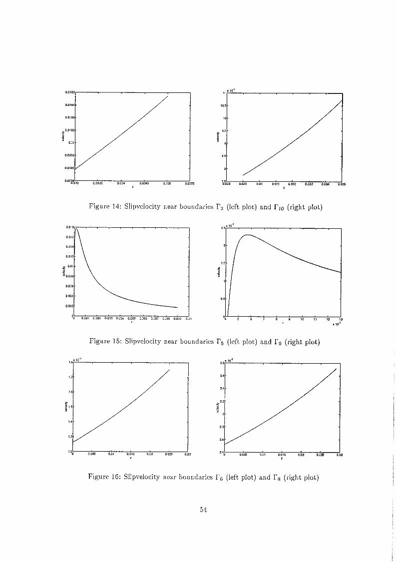
Figure 14: Slipvelocity near boundaries r2 (left plot) and rio (right plot)

O801 O802 0803 0804 0005 O806 0007 O808 O & l S O k

Figure 15: Slipvelocity near boundaries r5 (left plot) and I's (right plot)

L

Figure 16: Slipvelocity near boundaries r6 (left plot) and rs (right plot) I

I

54

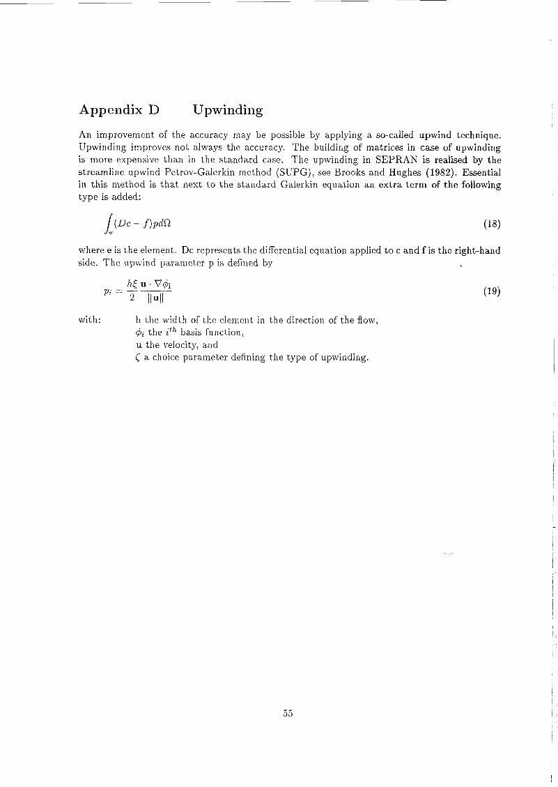
Appendix D Upwind iiig

An improvement of the accuracy may be possible by applying a so-called upwind technique. Upwinding improves not always the accuracy. The building of matrices in case of upwinding is more expensive than in the standa.rd case. The upwinding in SEPRAN is realised by the streamline upwind Petrov-Galerkin method (SUPG), see Brooks and Hughes (1982). Essential in this method is that next t o the standard Galerkin equation an extra term of the following type is added:

where e is the element. Dc represents the differential equation applied t o c and f i s the right-hand side. The upwind parameter p is defined by

with: h the width of the element i n the direction of the flow, 4i the i th basis function, u the velocity, and

a choice parameter defining the type of upwinding.

55

Re fer e lice s

[i] Geus, A.F.R. de On the design and manufa.cturing of oil-filled rubber dampers. Technical report W F W 94.07G, Eindlioven University of Technology, 1994

[a] Zoetelief, W.F. Multi-component Injection Moulding. Ph.D. thesis, ISBN 90-386-0016-X, Eindhoven University of Technology, 1995

[3] Segal, A. SEPRAN, user manual, standard problems and programming guide. 1ngenieursburea.u SEPRA, Leidschendam, The Netherlands, 1984

[4] Steenhoven, A.A. van De toepassing van de eindige elementenmethode bij stromingsproblemen. lecture notes, Eindhoven [Jniversity of Technology, The Netherlands, 1984

56