MULTI-INJECTOR MODELING OF TRANSVERSE COMBUSTION ...

Purdue UniversityPurdue e-Pubs

Open Access Theses Theses and Dissertations

Spring 2014

MULTI-INJECTOR MODELING OFTRANSVERSE COMBUSTION INSTABILITYEXPERIMENTSKevin "James " ShipleyPurdue University

Follow this and additional works at: https://docs.lib.purdue.edu/open_access_theses

Part of the Aerospace Engineering Commons

This document has been made available through Purdue e-Pubs, a service of the Purdue University Libraries. Please contact [email protected] foradditional information.

Recommended CitationShipley, Kevin "James ", "MULTI-INJECTOR MODELING OF TRANSVERSE COMBUSTION INSTABILITY EXPERIMENTS"(2014). Open Access Theses. 254.https://docs.lib.purdue.edu/open_access_theses/254

https://docs.lib.purdue.edu?utm_source=docs.lib.purdue.edu%2Fopen_access_theses%2F254&utm_medium=PDF&utm_campaign=PDFCoverPages

https://docs.lib.purdue.edu/open_access_theses?utm_source=docs.lib.purdue.edu%2Fopen_access_theses%2F254&utm_medium=PDF&utm_campaign=PDFCoverPages

https://docs.lib.purdue.edu/etd?utm_source=docs.lib.purdue.edu%2Fopen_access_theses%2F254&utm_medium=PDF&utm_campaign=PDFCoverPages

https://docs.lib.purdue.edu/open_access_theses?utm_source=docs.lib.purdue.edu%2Fopen_access_theses%2F254&utm_medium=PDF&utm_campaign=PDFCoverPages

http://network.bepress.com/hgg/discipline/218?utm_source=docs.lib.purdue.edu%2Fopen_access_theses%2F254&utm_medium=PDF&utm_campaign=PDFCoverPages

https://docs.lib.purdue.edu/open_access_theses/254?utm_source=docs.lib.purdue.edu%2Fopen_access_theses%2F254&utm_medium=PDF&utm_campaign=PDFCoverPages

01 14

PURDUE UNIVERSITY GRADUATE SCHOOL

Thesis/Dissertation Acceptance

Thesis/Dissertation Agreement.Publication Delay, and Certification/Disclaimer (Graduate School Form 32)adheres to the provisions of

Department

Kevin J. Shipley

MULTI-INJECTOR MODELING OF TRANSVERSE COMBUSTION INSTABILITYEXPERIMENTS

Master of Science in Aeronautics and Astronautics

William Anderson

Stephen Heister

Venke Sankaran

William Anderson

Wayne Chen 04/15/2014

i

MULTI-INJECTOR MODELING OF TRANSVERSE COMBUSTION INSTABILITY EXPERIMENTS

A Thesis

Submitted to the Faculty

of

Purdue University

by

Kevin J. Shipley

In Partial Fulfillment of the

Requirements for the Degree

of

Master of Science in Aeronautics and Astronautics

May 2014

Purdue University

West Lafayette, Indiana

ii

To my family and my teachers

iii

ACKNOWLEDGEMENTS

I would like to first thank my advisor, Professor William Anderson, for his

encouragement and guidance during my time at Purdue. He offered me an amazing

opportunity to explore the fascinating world of combustion instability and was always

there when I needed help. He has had a profound impact and I cannot thank him enough.

I would also like to thank Venke Sankaran. His advisement has been invaluable in

guiding me through the use of computational fluid dynamics and I am very grateful for

his insight. I must also thank Matthew Harvazinski for the immeasurable amount of time

and patience he has spent teaching me the skills to apply computational fluid dynamics.

What I have accomplished would not have been possible without him.

Thank you also to Cheng Huang, Swan Sardeshmukh and Changjin Yoon for your

continuous support throughout my research. Your talents have helped me learn so much

and I will always be grateful for the help you have given me.

The hands on learning I have had at Purdue is also something I am very grateful

for. So thank you Scott Meyer and Rob McGuire for taking the time to teach me about

designing and building rocket test stands. And thank you to Collin Morgan, Thomas

Feldman, Matthew Wierman, Michael Bedard, Rohan Gejji, Chris Fugger, and Brandon

Kan. You all have helped me learn how to setup and run tests and have given me many

great memories.

iv

I must also thank my family. I would not be where I am today without the love

and support they have given me. I am very lucky to have such wonderful people in my

life. And I must also thank two other wonderful people, Laura and Patrick with whom I

have gone on many great adventures. They both have made my time here amazing. I

cannot say thank you enough to everyone who has made this such a great experience and

I am happy to have been able to share this time with you.

v

TABLE OF CONTENTS

Page

LIST OF FIGURES ........................................................................................................... ix

ABSTRACT ............................................................................................................ xiv

CHAPTER 1. INTRODUCTION ................................................................................. 1

1.1 Background ............................................................................................... 1

1.2 Influences on Combustion Instability ....................................................... 4

1.2.1 Coaxial Injectors .................................................................................5

1.2.2 Flame Flowfield Interactions ..............................................................7

1.3 Prior Experimental Work .......................................................................... 9

1.4 Prior Modeling of Combustion Instability .............................................. 15

1.5 Objectives and Overview ........................................................................ 17

CHAPTER 2. EXPERIMENTS .................................................................................. 21

2.1 Second Generation Experiment ............................................................... 21

2.1.1 Experiment setup ...............................................................................23

2.1.2 Combustion Instability Measurements ..............................................25

2.2 3rd Generation Experiment ...................................................................... 27

2.3 Results ..................................................................................................... 28

2.3.1 Dynamic Mode Decomposition ........................................................36

CHAPTER 3. MODELING APPROACH ................................................................. 41

3.1 Computational Solver .............................................................................. 42

3.1.1 Turbulence Modeling ........................................................................44

vi

Page

3.1.2 Reacting Flow ...................................................................................46

3.1.3 Data Output .......................................................................................48

3.2 Three Injector Setup ................................................................................ 48

3.2.1 Geometry and Grid Generation .........................................................49

3.2.2 Boundary conditions and initial conditions ......................................53

3.2.3 Reaction Kinetics ..............................................................................58

3.3 Seven Injector Setup ................................................................................ 60

3.3.1 Geometry and Grid Generation .........................................................61

3.3.2 Boundary Conditions and Initial Conditions ....................................63

3.3.3 Reaction kinetics ...............................................................................65

CHAPTER 4. COMPUTATIONAL ANALYSIS OF INJECTOR RESPONSE ....... 66

4.1 Startup ..................................................................................................... 67

4.2 Instability Cycle ...................................................................................... 70

4.2.1 Ignition Study Application ................................................................72

4.2.2 Velocity Forcing Amplitude Effect ...................................................73

4.3 Comparison with Experiments ................................................................ 78

4.3.1 Pressure Comparison with Experiments ...........................................79

4.3.2 Injector Combustion Response Comparison .....................................85

4.3.3 Reaction Investigation .......................................................................90

4.4 Conclusion ............................................................................................... 96

CHAPTER 5. COMPUTATIONAL STUDY OF TRANSVERSE INSTABILITY MECHANISMS ............................................................................................................. 98

5.1 Overview of Instability Behavior ............................................................ 99

5.2 Startup ................................................................................................... 101

5.3 Low Amplitude Instability .................................................................... 106

5.3.1 Injector Response ............................................................................109

vii

Page

5.4 High Amplitude Instability.................................................................... 111

5.5 Conclusion ............................................................................................. 117

CHAPTER 6. SUMMARY ...................................................................................... 119

6.1 Conclusions ........................................................................................... 120

6.2 Recommendations ................................................................................. 122

REFERENCES ........................................................................................................... 124

viii

LIST OF TABLES

Table .............................................................................................................................. Page

Table 2.1: Second generation TIC configurations. O represents bipropellant flow and X represents oxidizer only flow. ........................................................................................... 23

Table 2.2: Operating conditions for each of the three configurations of interest. ............ 25

Table 3.1: Mesh quality metrics for the three-injector mesh. ........................................... 53

Table 3.2: Mass flow inlet boundary conditions for the three injector model. ................. 54

Table 3.3: Ethane model reaction parameters. .................................................................. 59

Table 3.4: Seven injector mesh quality. ............................................................................ 63

Table 3.5: Mass flow inlet boundary conditions for the seven injector model. ................ 64

Table 3.6: Single Step Methane Reaction Parameters. ..................................................... 65

Table 4.1: Instability amplitudes for 5, 23.5 and 35 m/s forcing ...................................... 74

Table 4.2: Pressure fluctuation amplitude and frequency comparison between the three injector simulations and experiments from a pressure measurement at the side wall ...... 80

ix

LIST OF FIGURES

Figure ............................................................................................................................. Page

Figure 1.1: Example coaxial injector with gaseous oxidizer through the central core and a swirled liquid fuel injected downstream [19]. .................................................................... 5

Figure 1.2: Continuously Variable Resonance Combustor (CVRC) [30]. ....................... 10

Figure 1.3: Transverse Instability Combustor, Generation 1with all gas-centered swirl coaxial injectors [31]. ........................................................................................................ 12

Figure 1.4: Second Generation Transverse Instability Combustor (right), Study Oxidizer Choke Piece (top left), Study Fuel Injector (left). ............................................................ 13

Figure 1.5: Generation III Transverse Instability Combustor with variable oxidizer post lengths and an increased window area. ............................................................................. 14

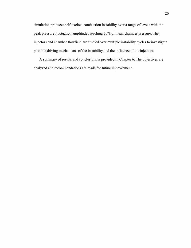
Figure 2.1: Second generation transverse instability combustor (right), study oxidizer choke piece (top left), study fuel injector (left). ............................................................... 22

Figure 2.2: System pressures and testing sequence. ......................................................... 24

Figure 2.3: Experiment measurements: CH* chemiluminescence (top left), high frequency pressure signal (bottom left), pressure transducer locations (right). ................ 26

Figure 2.4: Third generation transverse instability chamber experimental setup. Blue arrows indicate oxidizer flow and yellow arrows signify fuel flow. ................................ 27

Figure 2.5: Power spectral density plots of wall pressure taken at port 7 for configuration 1 (left), 2 (middle), 3 (right). ............................................................................................. 29

Figure 2.6: Sidewall bandpassed pressure signal for configuration 1 (left), configuration 2 (middle) and configuration 3 (right). ................................................................................ 29

Figure 2.7: Band-pass decomposition of high-pass filtered wall pressure for the first configuration (bottom) and second configuration (top). ................................................... 31

Figure 2.8: Transverse pressure trace across the chamber. ............................................... 32

x

Figure ............................................................................................................................. Page

Figure 2.9: Center injector response over a half cycle – configuration 1 pressure waveform and transverse velocity (first column). Dots on the plot indicate transducer measurements and the window lies between the black lines. CH* plots for configuration 1 (second column), 2 (third column), and 3 (fourth column). The time interval between rows is 50 μs. .................................................................................................................... 35

Figure 2.10: Dynamic mode decomposition of CH * - Pressure and transverse velocity waveform (column a), CH* DMD mode 1W (column b), 2W band-passed pressure and velocity waveform (column c), CH* DMD mode 2W. The white arrows show the general direction of the CH* zones. .............................................................................................. 39

Figure 3.1: Computational domain for the simulation and grid mesh. ............................. 50

Figure 3.2: Three injector model mesh. ............................................................................ 51

Figure 3.3: Primary velocity (left) and pressure (right) mode shapes in the three injector simulation. ......................................................................................................................... 55

Figure 3.4: Effect of wall velocity on pressure fluctuations at the side wall. ................... 56

Figure 3.5: Pressure mode shapes for the 1st (left column) and 2nd (right column) modes. Each row represents a different wall velocity boundary condition: 23.5m/s (top), 30 m/s (middle), 35 m/s (bottom), experimental data from port 7 – 10 is overlaid in blue. ........ 57

Figure 3.6: Ignition delay comparison between simulations with the original Arrhenius factor (green), modified Arrhenius factor (blue) and experimental data (red) [77]. ......... 60

Figure 3.7: Seven injector model geometry. ..................................................................... 62

Figure 3.8: Seven injector mesh geometry with a zoomed view of the center injector and adjacent oxidizer injector. ................................................................................................. 63

Figure 4.1: Ignition in the three injector simulation showing reactions from the central study injector and between the bypass flow and side oxidizer streams. The experiment window size is plotted in white. ........................................................................................ 67

Figure 4.2: Unforced flowfield conditions in the three injector simulations of ethane fuel, oxygen and heat release (top row) with zoomed in views (second row). Pressure, temperature and vorticity are shown in a full view (third row) and near the injection plane (fourth row). ...................................................................................................................... 69

Figure 4.3: Growth to limit cycle for different wall velocity boundary conditions in the three injector simulations. The measurement point is taken at the combustor side wall. . 70

xi

Figure ............................................................................................................................. Page

Figure 4.4: Simulation slices of pressure (top row), temperature (middle row), and heat release (bottom row) over a full instability cycle for the 30 m/s wall velocity case. The white ovals indicate the heat release elongation zone and the white arrows point to the heat release zone that that does not react strongly to the transverse wave ....................... 72

Figure 4.5: Effect of reducing the Arrhenius facto two orders of magnitude on time-averaged heat release. The reduced reaction rate case is shown on the left and the original faster reaction case is shown on the right ......................................................................... 73

Figure 4.6: Transverse velocity mode shape across the chamber width for varying forcing conditions. ......................................................................................................................... 74

Figure 4.7: Heat release fluctuation mode shape across the chamber width for varying forcing conditions. ............................................................................................................ 75

Figure 4.8: Effect of varying wall velocity amplitudes on the temperature flowfield using time-averaged results over 5 instability cycles. ................................................................ 75

Figure 4.9: Effect of varying wall velocity amplitudes on local ethane fuel mass fraction using time-averaged results over 5 instability cycles. Ethane isosurfaces are shown at 85%, 25% and 10%. .......................................................................................................... 77

Figure 4.10: Effect of varying wall velocity amplitudes on oxidizer mass fraction using time-averaged results over 5 instability cycles. Oxygen isosurfaces are shown at 10%, 20% and 30% .................................................................................................................... 77

Figure 4.11: Time averaged plots of heat release for different wall velocity conditions with an isosurface at 1.0E+10 W/m3. ............................................................................... 78

Figure 4.12: PSD analysis of the left wall pressure signal for varying velocity amplitude boundary conditions and experiment configurations low, medium and high. .................. 81

Figure 4.13: Band-passed wall pressure filtered at the four acoustic modes in the combustor for the experiment low (bottom left), medium (middle left) and high (top left) instability cases and the CFD simulations with a 5 m/s (bottom right) 23.5 m/s (middle right) and 30 m/s (top right) velocity amplitude boundary conditions. The signals are normalized by the mean chamber pressure. ...................................................................... 83

Figure 4.14: Decomposed wave form comparison between experiment test 17 (left) and CFD simulation (right) for WV = 30 m/s. The high pass filtered signal is shown in black and the summed band-passed modes are shown in orange. .............................................. 84

xii

Figure ............................................................................................................................. Page

Figure 4.15: Dynamic mode decomposition at the first acoustic mode of heat release in the simulation and CH* in the experiment. Simulation results are presented for the 30 m/s wall velocity case with a faster reaction and slower reaction achieved by adjusting the Arrhenius factor. The corresponding pressure and transverse velocity profile in the chamber for each time point is shown for reference. The white arrows show the direction the heat release is moving to. ............................................................................................ 88

Figure 4.16: Dynamic mode decomposition at the second acoustic mode of heat release in the simulation and CH* in the experiment. Simulation results are presented for the 30 m/s wall velocity case with a faster reaction and slower reaction achieved by adjusting the Arrhenius factor. The corresponding pressure and transverse velocity profile in the chamber for each time point is shown for reference. ........................................................ 89

Figure 4.17: Dynamic mode decomposition at the first acoustic mode for the 30 m/s wall velocity cases with a faster reaction and slower reaction achieved by adjusting the Arrhenius factor. Fuel (orange) and oxidizer (white) mass fraction are overlaid for each case to illustrate the relationship with the reacting zones. The time point for each row is the same as the rows presented in Figure 4.15 and Figure 4.16. ...................................... 92

Figure 4.18: Dynamic mode decomposition at the first acoustic mode for the 30 m/s wall velocity cases with a faster reaction and slower reaction achieved by adjusting the Arrhenius factor. Fuel (orange) and oxidizer (white) mass fraction are overlaid for each case to illustrate the relationship with the reacting zones. The time point for each row is the same as the rows presented in Figure 4.15 and Figure 4.16. ...................................... 95

Figure 5.1: Overview of instability produced in the seven injector simulaiton showing wall pressure fluctuations (top) and the corresponding freqency content (bottom). ........ 99

Figure 5.2: Left wall high-pass filtered pressure and band-pass filtered pressure at the three modes. .................................................................................................................... 100

Figure 5.3: Simulation startup from initial conditions. The combustor chokes almost immediately (shown left), ignites and produces a pressure wave that reflects of the nozzle and builds into a pressure spike (shown right) upon interaction with fuel entrained vortices downstream of the injector plane. ..................................................................... 102

Figure 5.4: Left and right wall pressure measurements showing transition from post-ignition to low amplitude combustion instability ........................................................... 103

Figure 5.5: As fuel and oxidizer fill the chamber pressure fluctuates in the chamber. .. 103

Figure 5.6: Initial pressure spike sources occur due to flame impingement on the side walls. The impingement points occur at the chamber side walls and converging section ............................................................................................................................. 104

Figure 5.7: Vortex first reaches the right wall and starts burning .................................. 105

xiii

Figure ............................................................................................................................. Page

Figure 5.8: Upon further mixing between fuel (left) and oxidizer (middle) the impinged vortex produces a stronger amount of heat release ......................................................... 105

Figure 5.9: Pressure oscillations at the left and right wall during a lower level of instability......................................................................................................................... 106

Figure 5.10: Pressure, axial velocity and transverse velocity at the left injector during low amplitude instability ........................................................................................................ 107

Figure 5.11: The low amplituide instability driving cycle shows how pressure and heat release pulsations are produced by flame and vorticy impingement with the side wall. 108

Figure 5.12: Axial velocity, pressure and transverse velocity band-passed at the main acoustic modes of the four injectors show the influence of the chamber instability at the transfer point to the injector. The red dashed line indicates the minimum transverse velocity, maximum pressure and maximum axial velocity for injector 1. ...................... 110

Figure 5.13: Averaged flow field plots from 2.5 – 5 ms of temperature (left) vorticity (middle) and heat release (right) show how the instability pushes flow from the side injectors to the middle and vorticity displacement along the wall with heat release. ..... 111

Figure 5.14: The pressure fluctuations transition from low level instability to high level instability around 7.4 ms. This is reflected in the pressure trace at both side walls. ...... 112

Figure 5.15: Average from 10 -12.5 ms .......................................................................... 113

Figure 5.16: Pressure, axial velocity and transverse velocity fluctuations at the left injector during high instability. ....................................................................................... 114

Figure 5.17: At higher instabilities vortices impinge between injector elements and may further drive the instability to stronger amplitudes. ........................................................ 115

Figure 5.18: Instability grows to the point that two strong pressure waves appears in the chamber. The dotted black line marks the corresponding point in time of the pressure and vorticity contours. ........................................................................................................... 116

Figure 5.19: Attenuation of the instability in the pressure measurements at the left and right wall as the additional wave reduces the coupling mechanisms present in the chamber. .......................................................................................................................... 117

xiv

ABSTRACT

Shipley, Kevin, J. M.S.A.A., Purdue University, May 2014. Multi-Injector Modeling of Transverse Combustion Instability Experiments. Major Professor: William E. Anderson.

Concurrent simulations and experiments are used to study combustion instabilities in a

multiple injector element combustion chamber. The experiments employ a linear array of

seven coaxial injector elements positioned atop a rectangular chamber. Different levels of

instability are driven in the combustor by varying the operating and geometry parameters

of the outer driving injector elements located near the chamber end-walls. The objectives

of the study are to apply a reduced three-injector model to generate a computational test

bed for the evaluation of injector response to transverse instability, to apply a full seven-

injector model to investigate the inter-element coupling between injectors in response to

transverse instability, and to further develop this integrated approach as a key element in

a predictive methodology that relies heavily on subscale test and simulation. To measure

the effects of the transverse wave on a central study injector element two opposing

windows are placed in the chamber to allow optical access. The chamber is extensively

instrumented with high-frequency pressure transducers. High-fidelity computational fluid

dynamics simulations are used to model the experiment. Specifically three-dimensional,

detached eddy simulations (DES) are used. Two computational approaches are

investigated. The first approach models the combustor with three center injectors and

xv

forces transverse waves in the chamber with a wall velocity function at the chamber side

walls. Different levels of pressure oscillation amplitudes are possible by varying the

amplitude of the forcing function. The purpose of this method is to focus on the

combustion response of the study element. In the second approach, all seven injectors are

modeled and self-excited combustion instability is achieved. This realistic model of the

chamber allows the study of inter-element flow dynamics, e.g., how the resonant motions

in the injector tubes are coupled through the transverse pressure waves in the chamber.

The computational results are analyzed and compared with experiment results in the time,

frequency and modal domains.

Results from the three injector model show how applying different velocity forcing

amplitudes change the amplitude and spatial location of heat release from the center

injector. The instability amplitudes in the simulation are able to be tuned to experiments

and produce similar modal combustion responses of the center injector. The reaction

model applied was found to play an important role in the spatial and temporal heat

release response. Only when the model was calibrated to ignition delay measurements did

the heat release response reflect measurements in the experiment. In this way, the use of

this approach as a tool to investigate combustion response is demonstrated.

Results from the seven injector simulations provide an insightful look at the possible

mechanisms driving the instability in the combustor. The instability was studied over a

range of pressure fluctuations, up to 70% of mean chamber pressure produced in the self-

exited simulation. At low amplitudes the transverse instability was appeared to be

supported by both flame impingement with the side wall as well as vortex shedding at the

primary acoustic frequency. As instability level grew the primary supporting mechanism

xvi

appeared to shift to just vortex impingement on the side walls and the greatest growth

was seen as additional vortices began impinging between injector elements at the primary

acoustic frequency.

This research reveals the advantages and limitations of applying these two modeling

techniques to simulate multiple injector experiments. The advantage of the three injector

model is a simplified geometry which results in faster model development and the ability

to more rapidly study the injector response under varying velocity amplitudes. The

possibly faster run time is offset though by the need to run multiple cases to calibrate the

model to the experiment. However, the model is also limited to studying the central

injector response and cannot capture any dynamic interactions with the outer injectors.

The advantage of the seven injector model is that the whole domain can be explored to

provide a better understanding about influential processes but requires longer

development and run time due to the extensive gridding requirement. Both simulations

have proven useful in exploring transverse combustion instability and show the need to

further develop subscale experiments and companions simulations in developing a full-

scale combustion instability prediction capability.

1

CHAPTER 1. INTRODUCTION

1.1 Background

Combustion instability is considered one of the main technical risks during rocket engine

development programs and as of yet no methodology exists to predict combustion

instability a priori in a full-scale engine. A system proven to be stable through testing

may undergo a small design alteration or operation change and suddenly show signs of

combustion instability [1, 2]. Instabilities can cause irreparable damage in a matter of

seconds; past examples include melted injector faces and nozzles that were torn apart [1].

Affordability is a major concern for new rocket engine designs and combustion

instability needs to be better understood to reduce the time and cost of development

programs. Recent advancements in computational fluid dynamics (CFD) modeling are

helping to promote a further understanding about how combustion instability arises. The

focus of this research is on applying CFD to simulate high-frequency combustion

instabilities in liquid rocket engines. Specifically, this work focuses on transverse

combustion instability in a multi-injector rocket combustor called the transverse

instability combustor, or TIC. Comparisons are also made with companion experiments.

Combustion instability has historically been classified into low- or high-frequency

instabilities. Low-frequency instabilities, often termed chug or pogo instabilities have

2

frequencies on orders of several hundred hertz or lower. The low-frequency instabilities

are generally linked with the propellant feed system or launch vehicle structure and

forces on the vehicle [3]. The cause is fundamentally different for high-frequency

instability which occurs above 1000 Hz and is related to acoustic coupling in the

combustion chamber. The focus of this work is on high-frequency combustion instability;

hence forth any reference to combustion instability will imply high-frequency

combustion instability.

High-frequency combustion instability arises when the heat release from

combustion couples with acoustic modes of a chamber. While present in all combustion

devices liquid rocket engines are particularly susceptible. During naturally-unsteady

combustion, acoustic waves are produced that reflect off the chamber walls and interact

with the reacting flowfield. The acoustics serve as a feedback mechanism, influencing

combustion which may in turn amplify or attenuate the acoustic waves. This coupling is

dependent on many factors including the method of propellant injection, flowfield

structure, combustor geometry and their influence on one another.

High-frequency instabilities can occur in either longitudinal or transverse modes as

well as spinning or mixed modes. A longitudinal instability is characterized by waves

which travel along the main combustor axis. These waves reflect back and forth between

the injector face and converging-diverging nozzle. In a transverse instability waves

instead propagate perpendicularly to the axial flow, reflecting off the chamber side-walls.

The transverse modes are generally considered to be the more destructive of the two.

This destructive power was especially evident in development of the F1 engine

which was used in the Saturn V rocket. During the development and testing phase the

3

engine was plagued with strong combustion instabilities. While the instability was

ultimately eliminated, doing so added four years to the program and required over 2000

full-scale tests out of the 3200 run during development [4]. Despite much work over the

past several decades the phenomena of combustion instability is not completely

understood.

New capabilities are arising however in the field of computational fluid dynamics

that can help move away from empirical methods of modeling combustion instability to

physics based models. The key has been the application of large eddy simulations (LES)

or hybrid forms of LES. Studies have shown that LES allows for coupling between the

combustion heat release and the acoustics of the geometry to be modeled [5 - 12]. The

reason LES is so crucial is because it allows large-scale eddies to be resolved which

appears to play a large part in the reacting flow dynamics.

Limitations still exist in these models however. Not all of the physical processes

are able to be modeled accurately and comparisons with experiments are limited due to

available experimental measurement techniques. Computational run-time is another issue,

since the large unsteady calculations may take several months to complete. Currently it

is still too expensive to simulate a full-scale engine with CFD.

An alternative approach is to employ CFD simulations with subscale experiments

to investigate combustion instabilities under variable geometries and operating

conditions. This is the approach this research applies. The subscale experiments are

designed to match parameters like performance, stability, heat transfer and ignition in full

scale systems. And although not all physical and chemical processes are matched exactly,

subscale testing is less expensive and allows for detailed measurements. To extend results

4

to full-scale engines, data from experiments and validated CFD simulations can be used

for developing combustion response functions for input into engineering-level design

analysis models. This approach has been partly developed by Krediet [13] using

combustion response functions extracted from OpenFOAM simulations.

1.2 Influences on Combustion Instability

Combustion instability is typically tied to the propellant injection system in an

engine. This is because the injection system affects the spatiotemporal behavior of heat

release in the combustion chamber. Mechanisms that occur at temporal scales similar to

acoustic time scales are generally those capable of driving combustion instability. A

particular process of interest in this study is how acoustic coupling of coaxial injectors

affects the flame flowfield interactions in a combustion chamber. The particular

mechanism which this process is theorized to affect is vortex generation. Mechanisms

which are more difficult to model, such as atomization and vaporization, have also been

demonstrated to drive combustion instability [14 - 17], and even chemical reaction time

scales have been found to couple with acoustics [18]. Many of these processes, which

may play a role in the experiments remain beyond our current ability to fully represent in

CFD simulations. The focus of the present research is on the coupling between the fluid

mechanics and acoustics in a gas-gas system, while employing relative simple global

kinetics mechanisms for the combustion chemistry.

5

1.2.1 Coaxial Injectors

The use of coaxial injectors was made popular by Russian engineers in the design of

oxidizer rich staged combustion (ORSC) liquid rocket engines. Figure 1.1 shows an

example coaxial injector configuration. The figure depicts oxidizer flowing axially

through the central core of the injector. Fuel is injected through an annulus just upstream

of the combustion chamber separated from the oxidizer. The fuel enters the flow parallel

to the core flow; in this region, if the fuel is a liquid it will atomize due to a Kelvin-

Helmholtz instability. During atomization the fuel and oxidizer also begin to mix and

vaporize in what is called the vortex chamber. The vortex chamber acts as a shield for

these processes from transverse acoustic oscillations.

Figure 1.1: Example coaxial injector with gaseous oxidizer through the central core and a swirled liquid fuel injected downstream [19].

6

The injectors used in this research are based off the Russian design used in the NK-33

and RD-170 engines [20]. Coaxial injectors are found in two varieties, swirl coaxial

injectors and shear coaxial injectors. In a swirl coaxial injector either the fuel, oxidizer or

both are injected with a swirl component. In the case of shear coaxial injector the oxidizer

and fuel streams are swirl free. In the present work a shear-coaxial set-up is used with a

gaseous oxidizer core and gaseous fuel. This is advantageous because the injectors act as

acoustic resonators. By changing the resonator length the injector can be sized to match

the chamber acoustics. The similarity in the temporal scale of the chamber acoustics and

injection time scale allows a coupling between the acoustically-induced flow oscillations

in the oxidizer tube, chamber acoustics, and heat release to develop.

The coaxial injectors in the TIC experiment play an important role on the

combustor’s instability and it is important to understand what influences their

performance. Under certain conditions of the fuel and oxidizer momentum ratio and the

pressure drop, coaxial injectors have been found to produce self-oscillations. These

oscillations can serve as a source for the heat release oscillations [21, 22]. Swirling either

the fuel or oxidizer has also been found to affect performance. Swirling is believed to

reduce sensitivity by stabilizing the outer flow while shear coaxial injectors have been

found to be more sensitive to pressure and velocity fluctuations [20].

The effect of swirl and momentum ratio play an important role in vortex formation,

which is considered one of the driving mechanisms in the combustor and will be

discussed in the next section. Deviation of the momentum ratio from one between fuel

and oxidizer in 2D axisymmetric simulations of coaxial injectors was found to increase

vortex shedding frequency, and if swirled the flow developed wake oscillations [19, 23].

7

Coaxial injectors have a large impact on developing vortical structures through either

geometry or flow parameters.

1.2.2 Flame Flowfield Interactions

Interactions between the unsteady flowfield and flame can have a direct impact on

the presence and amplitude of a combustion instability. Combustion instability has been

theorized to be driven by vortex interactions. Smith and Zukowski [24] first demonstrated

that vortices can serve as a source to feed energy into the acoustic field that may sustain

combustion instability. The vortices were formed during a propellant injection under

large velocity fluctuations. Once formed, the vortices entrain incoming fuel and are

convected downstream, igniting at a later time. The vortices have been shown to ignite

once impinging on another vortex or surface boundary [25]. This rapidly changes the

flame surface area and a pressure pulse is produced [26]. The pulse feeds energy back

into the flowfield and the cycle continues as more velocity perturbations are produced,

causing more vorticity. Other sources of heat release perturbations were investigated by

Ducruix et. al. [26] who found that flame interactions on a wall, unsteady strain rates, and

fluctuating equivalence ratios could also feed energy into the acoustic field.

The process for vortex formation in the TIC is presented in Reference 27. It was

theorized that a vortex would be shed off the side injectors at a rate equal to the resonant

frequency of the chamber. The injector step height from the wall was then set so that the

vortex would impinge on the side wall when a pressure reached a maximum in that

location, thus feeding energy back into the acoustic field which would perpetuate the

cycle. Moreover, the length of the injector post elements were matched with the resonant

frequency of the chamber in order to support the incidence of combustion instability. This

8

approach was originally proven successful for exciting longitudinal modes [28, 29, 30]

and, more recently, extended to transverse modes [27, 31], i.e., the TIC configuration.

Additional details of these experiments are provided in the following section.

With the improving capability of modeling unsteady, reacting flows and the ability

to fully explore the computational domain, CFD helps provide further insight into

combustion instability mechanisms. Smith et al. [32, 33] performed 2D-axisymmetic

simulations of a single element combustor to study longitudinal instabilities. It was

shown that the instability mechanism was related to vorticity pulsing in the oxidizer post

and vorticity impingement on the chamber wall. A further investigation was made by

Harvazinski et al. [34] into the instability mechanisms using 3D simulations. Three

influential processes were identified in relation to the instability. The first process was the

timing of pressure pulses in the combustor and oxidizer post. The moving longitudinal

wave was observed to disrupt the fuel flow which allowed for heat release to move

downstream ultimately allowing fuel to accumulate upstream without burning. Then as

the fuel burned it was hit by the travelling wave, increasing heat release and pressure.

Other influential processes included increased mixing due to baroclinic torque which

produces vorticity due to misaligned pressure and density gradients and the effect of a

tribrachial flame. The tribrachial flame is made up of three layers: oxidizer, fuel and

burnt gases. The triple flame is a strong source for heat release as the burnt gases heat up

the unburnt oxidizer and fuel. The existence of the tribrachial flame was first identified

by Garby et. al. [12] and Guéezzenec [35] linked the movement and extinguishment of

the triple flame to the first acoustic mode. In other simulations Harvazinski [34] found

that the triple flames dynamics were more complex, moving throughout the combustor,

9

and were extinguished and reformed regularly. More background on the combustion

stability models are provided later.

1.3 Prior Experimental Work

Development of the TIC began with interest in ORSC engines. The Russians have

typically used uni-element testing to simulate combustion instability in full-scale ORSC

engines. This led to a set of experiments designed to investigate combustion instability at

Purdue. A swirl coaxial injector was developed based upon the RD-180 injector and

tested in a longitudinal combustor at a pressure antinode. The combustor was run with

90% decomposed hydrogen peroxide and hydrocarbon fuels, looking at the effects of

chamber length, oxidizer tube length, backstep height and oxidizer inlet conditions on

instability [28, 29].

From these initial studies, it was determined that having a strong pressure

antinode at the combustor head does not necessarily drive instability, and vortex shedding

was found to be the more likely mechanism for causing instability. Also, the injector was

found to be less important in taking away acoustic energy and more important in how

pressure and velocity are affected in the combustion zone [29].

The longitudinal combustor evolved into the continuously variable resonance

combustor (CVRC) where the injector oxidizer post lengths were varied continuously

during tests. In addition the experiment was modified to aid in comparison with

computational simulations by using gaseous methane fuel and changing the oxidizer

injection to an axisymmetric flow using a slotted choke plate [30]. An optical section was

10

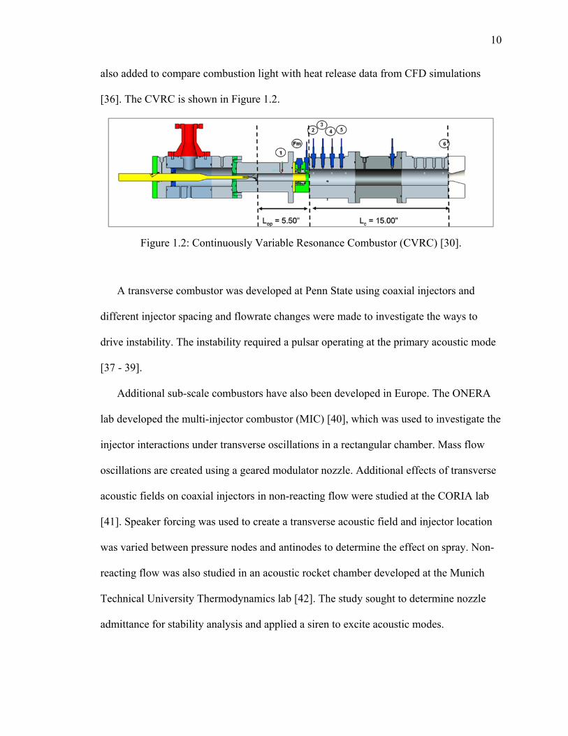
also added to compare combustion light with heat release data from CFD simulations

[36]. The CVRC is shown in Figure 1.2.

Figure 1.2: Continuously Variable Resonance Combustor (CVRC) [30].

A transverse combustor was developed at Penn State using coaxial injectors and

different injector spacing and flowrate changes were made to investigate the ways to

drive instability. The instability required a pulsar operating at the primary acoustic mode

[37 - 39].

Additional sub-scale combustors have also been developed in Europe. The ONERA

lab developed the multi-injector combustor (MIC) [40], which was used to investigate the

injector interactions under transverse oscillations in a rectangular chamber. Mass flow

oscillations are created using a geared modulator nozzle. Additional effects of transverse

acoustic fields on coaxial injectors in non-reacting flow were studied at the CORIA lab

[41]. Speaker forcing was used to create a transverse acoustic field and injector location

was varied between pressure nodes and antinodes to determine the effect on spray. Non-

reacting flow was also studied in an acoustic rocket chamber developed at the Munich

Technical University Thermodynamics lab [42]. The study sought to determine nozzle

admittance for stability analysis and applied a siren to excite acoustic modes.

11

The German Aerospace Center (DLR) has also developed a set of subscale

experiments, including the common research combustor (CRC) which is jointly operated

with the French National Center for Scientific Research (CNRS). The CRC is a flat

cylindrical combustor with radial injector mounting. And like the MIC, flow is modulated

with a siren and secondary nozzle. [43, 44]. Two other experiments at DLR are the BKH

and BKD combustors. The BKH is similar to the MIC with a rectangular chamber and

siren excitation but applies coaxial injectors in a matrix form and is designed to

investigate LOX/H2 reactions at higher pressures [45, 46]. The BKD is a cylindrical

combustor without external forcing and is more representative of a multi-injector engine

with 42 shear coaxial injector elements [47].

All previous rectangular combustors have used an external forcing mechanism to

excite instability. The TIC at Purdue was developed without an external forcing

mechanism, applying the principles of vortex shedding learned in the longitudinal CVRC

combustor [48]. With this approach, chamber conditions may be considered more

representative of actual rocket engine combustion chambers without the outside influence

of the external forcing mechanism.

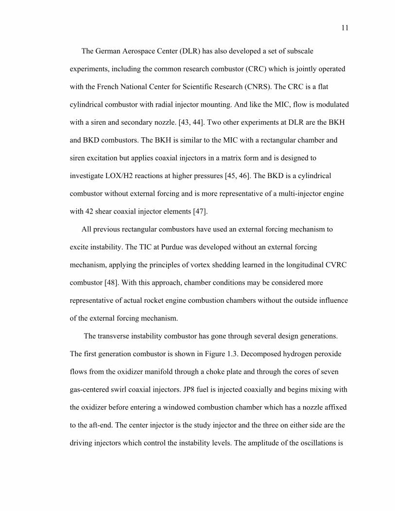
The transverse instability combustor has gone through several design generations.

The first generation combustor is shown in Figure 1.3. Decomposed hydrogen peroxide

flows from the oxidizer manifold through a choke plate and through the cores of seven

gas-centered swirl coaxial injectors. JP8 fuel is injected coaxially and begins mixing with

the oxidizer before entering a windowed combustion chamber which has a nozzle affixed

to the aft-end. The center injector is the study injector and the three on either side are the

driving injectors which control the instability levels. The amplitude of the oscillations is

12

controlled by selecting which of the driving injectors flow bipropellant (fuel and

oxidizer) and which flow only oxidizer.

Figure 1.3: Transverse Instability Combustor, Generation 1with all gas-centered swirl coaxial injectors [31].

Pomeroy investigated the instability effects on the center injector, taking high frequency

pressure measurements, backlit and CH* chemiluminescent images through the chamber

window [49]. Backlit images provide a look at the flowfield downstream of the center

injector and the CH* chemiluminescent images provide a qualitative measure of heat

release. Results showed that the study injector would couple with the first velocity mode.

At higher instabilities the fuel would be displaced into an oxidizer rich region and

combust. But under lower instabilities the oxidizer and not the fuel was displaced.

The next generation combustor was developed by Morgan [27] and was designed

to provide data for comparison with high fidelity CFD simulations and was designed to

relate to conditions in the Air Force Hydrocarbon Boost main chamber. The combustor,

13

shown in Figure 1.4 has a redesigned center injector similar to that used in the CVRC.

The oxidizer choke piece is moved downstream to prevent pressure fluctuations from

coupling with the first acoustic mode of the chamber. The center, shear-coaxial fuel

injector injects gaseous ethane (shown in red) which more closely resembles supercritical

conditions. The gaseous fuel also allows for the CFD modeling to ignore atomization.

Decomposed hydrogen peroxide is used as the oxidizer and RP1 (shown in orange) is

injected through the outer swirl coaxial driving injectors. Like the previous generation the

instability level in the chamber is adjusted by flowing monopropellant or bipropellant

through the injectors.

Figure 1.4: Second Generation Transverse Instability Combustor (right), Study Oxidizer Choke Piece (top left), Study Fuel Injector (left).

The third generation combustor was designed to improve optical access to the

combustion region and allow for variable oxidizer tube lengths to investigate their effect

on the instability. By changing oxidizer tube lengths instead of changing fuel mass flow,

14

different instability levels can be investigated without varying species composition in the

combustor. The second generation window was increased from 2.45 in × 2.45 in to 3.25

in × 3.23 in. The oxidizer tubes are designed with individual choke plates that can be

replaced for studying different acoustic boundaries and the whole chamber is compressed

hydraulically. The first and second generation combustors relied on auto-ignition and

required a brass plate placed at the nozzle exit. This combustor relies on an igniter

running gaseous oxygen and hydrogen. The combustor was also designed for comparison

with high fidelity CFD simulations and runs on hydrogen peroxide and only methane

fuel.

Figure 1.5: Generation III Transverse Instability Combustor with variable oxidizer post lengths and an increased window area.

15

1.4 Prior Modeling of Combustion Instability

Once validated against experimental data CFD provides an opportunity to further

explore the physical and chemical processes that take place during unstable combustion.

Rapid growth in size and availability of computational resources over the past several

years allow for the modeling of complex physical phenomena.

Many simulations of combustion instability have employed forcing functions to

investigate modes of interest. Ellis [50] used a series of simulations in 1D, 2D and 3D to

study transverse combustion instability. In the simulations broadband forcing functions

were used to determine unstable modes. Results from those simulations showed higher

forcing amplitudes dampened higher order modes and viscosity also dampened

instability. Follow-on simulations by Smith et al. showed that viscosity is needed to

predict mode shapes and frequencies as well as nonlinear phenomena [51]. The viscous

simulations overall showed good qualitative agreement with similar amplitudes,

frequencies and mode shapes to the experiments. [38, 50]. The need to drive instability

through forcing may be an indication the underlying model is overly simplistic and lacks

key physics.

While direct numerical simulation (DNS) of combustion instability would provide

the most accurate solutions DNS remains too expensive for the large geometries of

interest in this work. The next level of fidelity is LES. In LES only large scale eddies are

resolved and sub-grid models are applied for scales unresolved by the grid. LES however

still requires a fine grid resolution and for complex simulations can be too expensive. In

fact lower fidelity models have been shown to outperform full LES simulations with

coarse grids [52]. Reynolds averaged Navier-Stokes (RANS) simulations typically

16

perform poorly for highly unsteady flows because the turbulence models produce too

much eddy viscosity and over-damp the unsteady motion of the fluid; since combustion

instability is an unsteady process RANS is not appropriate. A combination of RANS and

LES sometimes called hybrid RANS/LES or detached eddy simulations (DES) is a

turbulence modeling technique where LES is applied in the regions where the grid

resolution supports it and RANS is applied in the under-resolved regions (typically the

near wall region). This has the benefit of requiring less grid points than LES but

providing better capability for capturing unsteadiness than RANS alone, particularly in

the off-body regions where the combustion typically occurs.

The next advancement sought to answer the question whether the longitudinal

combustor simulations could exhibit growing unsteady heat release without forcing

functions and still match experiments. The simulations were 2D axisymmetric and ran

with global reaction mechanisms, the lowest order kinetics model. The effect of step

height and oxidizer tube length were investigated and it was found that axial velocity

fluctuations in the oxidizer post affected vorticity generation which occurred in phase

with pressure oscillations. And smaller backstep heights affected the location of vortex

impingement. Grid resolution had an impact on disturbance amplitude and in most cases

the instability did not match with the experiments [9, 32, 33]. The stable regimes were

over predicted and experimental unstable regimes were under predicted. 2D simulations

did not capture higher mode shapes.

As model complexity grew, so did the need to understand what affects modeling

parameters were having on simulation results. Further longitudinal combustor simulations

investigated what effects finer grid resolutions and more advanced reaction models had

17

on instability levels. Finer grid resolutions resulted in increased instability with more heat

release and closer matching of mode frequencies to experiments. And using multi-step

reaction mechanisms as opposed to single step mechanisms increased instability however

resulted in less accurate frequency modes in comparison to companion experiments [53].

This shows that modeling methods must be chosen carefully and when simulation results

are compared with experiments the possible effects need to be understood.

Simulations were taken to the next level of complexity, moving from 2D

axisymmetric to 3D simulations of the CVRC. The 3D simulations were found to capture

the higher harmonic modes yet limit cycle amplitudes were still less than the experiment

counterpart [11, 54]. And while the 5.5 in length oxidizer post case was unstable in both

the experiment and simulation, CFD models predicted the 7.5 in case would also be

unstable when in fact it was stable in the experiment [34], a result that is probably related

to the omission of wall heat transfer effects in the simulations. As mentioned previously

the CVRC used a slotted choke plate in the inlet which was modeled in the CFD

simulations. The effect of the choke plate was measured against a simple mass flow inlet.

Results showed applying the simple mass flow inlet led to higher instabilities with higher

unmatched harmonic mode amplitudes. The size of the recirculation region and peak heat

release location changed, showing inlet boundary conditions must also be chosen

carefully [55]. The same choke plate is used in the center injector of the TIC simulations.

1.5 Objectives and Overview

CFD simulations have gone from simple 1D and 2D models requiring forcing

functions to full 3D simulations with self-excited combustion instability that match trends

18

seen in experiments. Even with the current state of complexity, model geometry is still

relatively basic and highly simplified chemical kinetics models are used. To date most

simulations have focused on longitudinal instabilities. This research focuses on transverse

instabilities. Specifically, the primary objectives of this research are to:

1. Develop a computational test bed for the evaluation and screening of

injector response to transverse instability using a reduced three-injector

model of the TIC configuration

2. Study the mechanisms for self-excited transverse instability generation on

the TIC setup using a full seven-injector model

3. Further develop the integrated subscale modeling and experimental

approach as a key element in a predictive methodology

The objectives reflect the capabilities of the two different models. The three injector

model is meant for studying the response of a single injector element under a range of

transverse instability amplitudes while the seven injector model supports an investigation

into all the injector responses and their influences. The three injector model is designed to

simulate the second generation experiment and the response of the center injector is

analyzed under transverse oscillations created by applying a velocity forcing function.

The seven injector model is designed to simulate the third generation experiment and a

velocity forcing is not applied as the instability is self-excited and driven by the physics

modeled.

In Chapter 2 setup of the second and third generation experiments are presented

which the simulations are designed after. The second generation experiment runs with

19

decomposed hydrogen peroxide, RP1, and ethane fuel while the third generation

experiment runs with decomposed hydrogen peroxide and methane. The effect of

different configurations on the pressure field in the second generation experiment is

analyzed as well as the injector response for later comparison with simulation results. The

injector response is studied using dynamic mode decomposition of the chemiluminescent

images taken.

In Chapter 3 the modeling approach is presented for the three injector and seven

injector models. Detail is given about the computational solver, grid geometry, boundary

conditions, initial conditions, and reaction kinetics. Both simulations are three-

dimensional detached eddy simulations. The three injector model excites instability via a

velocity forcing function while instability in the seven injector model develops through

the physics inherent in the model. An adjustment to the reaction model in the three-

injector model is also setup to investigate the effect on injector response.

Chapter 4 provides results from the three injector simulations. The focus of the

chapter is on analyzing how the center injector response is influenced by the model and

determining how well the simulation matches experiments. The instability cycle process

is presented and flowfield changes under different forcing amplitudes are analyzed. The

simulations are further compared with experiments, comparing both pressure field

measurements and combustion response. Dynamic mode decomposition is again applied

as a tool to simplify heat release comparison with the experiment on a modal basis. The

effect of a different reaction rate is further analyzed by similar methods.

In Chapter 5 the full seven-injector model is applied to investigate how injectors

previously found to be longitudinally unstably respond to transverse instabilities. The

20

simulation produces self-excited combustion instability over a range of levels with the

peak pressure fluctuation amplitudes reaching 70% of mean chamber pressure. The

injectors and chamber flowfield are studied over multiple instability cycles to investigate

possible driving mechanisms of the instability and the influence of the injectors.

A summary of results and conclusions is provided in Chapter 6. The objectives are

analyzed and recommendations are made for future improvement.

21

CHAPTER 2. EXPERIMENTS

The transverse simulations in this work are based on the second [27] and third generation

transverse instability combustor. This chapter is organized into sections describing setup

of the companion experiments from which boundary conditions in the CFD model were

derived from and results are also presented from the second generation experiment. The

focus of the analysis is on evaluating how different configurations produce changes in the

pressure field in the combustor and how the center injector responds for later comparison

with CFD simulations.

2.1 Second Generation Experiment

The transverse instability chamber, TIC, is an injector test bed which provides a

unique ability to study combustion subjected to transverse flow oscillations. The injector

of interest, referred to as the study injector or element, is placed at the center of the

chamber. Three driving injectors sit on each side of the driving element. Different

configurations of the driving injector yield varying levels of instability amplitude from

8% of the chamber pressure on the low end to 65% on the high end. The second

generation combustor is shown in Figure 2.1. The center study element was previously

used in a longitudinal setup and found by Yu et al. to be unstable [30].

22

Figure 2.1: Second generation transverse instability combustor (right), study oxidizer choke piece (top left), study fuel injector (left).

The level of instability in the chamber is controlled by setting flow type in the outer

driving injectors. Either a monopropellant or bipropellant is used. Instability results from

different operating configurations are shown in Table 2.1. In the table O represents

bipropellant flow while X indicates oxidizer-only flow through the injector. The elements

on either side of the study element flow only oxidizer in an effort to help isolate the study

element. The first configuration, which is the same as depicted in Figure 2.1 uses RP1

and decomposed peroxide for the fuel and oxidizer in in the outer four injectors. For the

study element gaseous ethane and decomposed peroxide are used for the fuel and

oxidizer respectively. The oxidizer only elements also use decomposed hydrogen

peroxide. This configuration gives the maximum chamber pressure (Pc) and the highest

amplitude pressure fluctuations (P’). By reducing the number of elements flowing

23

bipropellant configuration two and three have lower amplitude pressure fluctuations

compared to the first configuration. The primary acoustic frequency also changes for

each configuration. This is a result of different temperature flowfield between the

configurations which directly affects the speed of sound in the chamber.

Table 2.1: Second generation TIC configurations. O represents bipropellant flow and X represents oxidizer only flow.

No. Configuration Pc, kPa P’, kPa P’ /Pc, % 1W Frequency, Hz

1 OOXOXOO 965 620 65% 2032

2 OXXOXXO 830 415 50% 1807

3 XOXOXOX 815 70 8% 1855

2.1.1 Experiment setup

A pressure feed system supplies propellant to the experiment and a timing

sequence is set up to control when valves are opened and closed for propellant delivery.

The process can influence the amplitude of the instability and is important to know for

applying boundary and initial conditions in the CFD simulations. For each configuration

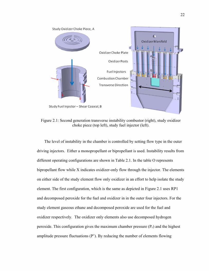
in Table 2.1 the timing sequence is identical. Figure 2.2 shows several pressure traces

with key points in the timing sequence identified. The first to be activated are the fuel

purges which begin at 1.5 seconds. During this event gaseous nitrogen flows through the

fuel injectors to prevent oxidizer from flowing into the fuel lines. The oxidizer is

decomposed through a catalyzer bed and a cavitating venturi is used to control the mass

flow rate. At 2 seconds the oxidizer run valve is opened allowing decomposed hydrogen

peroxide to fill the chamber. The flow of fuel is also controlled by cavitating venturis. At

3.5 seconds the study fuel run valve is opened and gaseous ethane is injected into the

24

chamber, ignition follows shortly thereafter. Four seconds later the valve supplying RP1

to the driving injectors is opened and RP1 quickly combusts in the chamber. Once the

driving injectors are active the center injector is subjected to transverse waves. The

unstable conditions are held in the combustor for approximately one second while

combustion instability measurements and data are taken. At the conclusion of the

measurement period fuel run valves are closed and the nitrogen purge is reactivated, and

the remaining oxidizer is purged through the chamber.

Time, s Event 1.5 – 7.5 Fuel Purge

2 - 15 Oxidizer fire 3.5 – 8.8 Study Fuel Fire 7.5 – 8.8 Fuel Driver fire8.8 - end Fuel Purge

Figure 2.2: System pressures and testing sequence.

Table 2.2 shows the measured propellant mass flows per injector and fuel temperature for

each configuration. Each bipropellant injector runs fuel rich while the overall equivalence

ratio of the combustor is oxidizer rich. The mass flows and temperatures are used as

boundary conditions for the companion CFD simulations.

25

Table 2.2: Operating conditions for each of the three configurations of interest.

Test Conditions Configuration 1 Test 17

Configuration 2, Test 39

Configuration 3, Test 23

Oxidizer (H2O2) Flow Rate Per Injector, kg/s

0.194 0.196 0.194

Driving fuel (RP1) flow rate per injector, kg/s

0.033 0.032 0.032

Study fuel (C2H6) flow rate per injector , kg/s

0.025 .025 0.024

Fuel Temperature, K 320 321 320

2.1.2 Combustion Instability Measurements

During the period of instability both pressure measurements and optical images of

combustion are taken. The pressure measurements are taken with high-frequency

transducers at a sampling rate of 100 kHz. The high frequency is needed to capture the

acoustic modes in the combustor, the lowest of which is around 2 kHz. The pressure

measurements are taken at the port locations shown in Figure 2.3. The ports were placed

at several important locations. Two ports were placed at the side walls where pressure

antinodes lie to detect the acoustic modes. Two transducers are also placed in the center

injector oxidizer tube, one near the choke piece and the second as near the injection plane

as was allowable. The other transducers are placed adjacent to the quartz window to

provide pressure data as the transverse wave travels across the chamber. They provide a

look at how the wave changes across the window and from wall reflections.

26

Figure 2.3: Experiment measurements: CH* chemiluminescence (top left), high frequency pressure signal (bottom left), pressure transducer locations (right).

The optical measurements are high-speed video of CH* chemiluminescence

through the center quartz window. CH* is a short lived radical that is created during the

combustion process and produces 431 nm [31] wavelength photons that can be captured

for viewing the reaction zone. High speed video of CH* is used to provide a qualitative

measure of heat release for comparison with CFD simulations. This technique for heat

release representation has been investigated in previous studies and has been shown to be

applicable [56], although others have found that CH* is not a good indicator of heat

release for certain flame environments [57]. In high-pressure environments, like those

found in the TIC, the CH* variation due to strain rate and equivalence ratio has been

found to be small [58 59].

27

2.2 3rd Generation Experiment

The third generation experiment is shown in Figure 2.4 and the setup is similar to

the second generation experiment. The fuel is switched to methane for both the driving

and study elements; the oxidizer is again decomposed hydrogen peroxide. The driving

injectors are changed to all shear coaxial injectors. The study injector matches the study

injector found in the second generation experiment. The oxidizer tube lengths and

chamber width remain unchanged. Oxidizer and fuel mass flow rates remain the same as

those presented in Table 2.2. The third-generation experiment is currently in progress and

the full seven-injector simulations presented in this thesis are a pre-cursor to associated

experimental tests. Similar high-frequency pressure measurements and high-speed CH*

video will also be taken for later comparison with the simulations.

Figure 2.4: Third generation transverse instability chamber experimental setup. Blue arrows indicate oxidizer flow and yellow arrows signify fuel flow.

28

2.3 Results

Results presented in this chapter are from the high-frequency pressure

measurements and CH* chemiluminescent images collected in the second generation TIC

[27]. The results show how the chamber acoustics and injector response changes for

different configurations. Dynamic mode decomposition is also performed on CH*

measurements from configuration one for later comparison with simulation results.

Analyzing frequency content in the pressure signal at the side walls shows how the

higher instability configurations produce stronger responses across multiple transverse

modes. The frequency content is determined from pressure measurements taken at the

side walls where acoustic antinodes lie for each mode. The frequency in the signal is

determined by performing a power spectral density (PSD) analysis. A PSD for the three

configurations is shown in Figure 2.5. The analysis is performed using 45 ms from the

limit cycle period. This yields a frequency resolution of 25 Hz and a maximum frequency

of 50 kHz.

Configuration one shows the largest amplitude with the first transverse mode

centered about 2026 Hz. Sharp well defined peaks are visible for each of the four modes

with the first mode having the highest amplitude. Modes two through four show smaller

amplitudes and are centered about integer multiples of the first mode. In the second

configuration the first mode has shifted to 1807 Hz and is 219 Hz lower than the first

configuration. The higher order modes are not as well defined in this case with broader

peaks. And the third configuration, with the lowest overall amplitude, shows less well

defined modes with the first and fourth mode having comparable amplitudes. As

instability grows in the TIC so too does the power in each mode.

29

Figure 2.5: Power spectral density plots of wall pressure taken at port 7 for configuration 1 (left), 2 (middle), 3 (right).

Comparing pressure antinode amplitudes further reveals how the first mode grows

the most between configurations and shows how the higher modes also grow but not to

the same degree. The pressure antinode amplitudes for each acoustic mode are

determined by band-passing the wall pressure signal at the frequencies identified in the

PSD analysis. The pressure is band-passed using a zero-phase shifted Butterworth filter

during the chamber limit cycle. The passband is set to ±5% of the frequency of interest.

Figure 2.6 shows the band-passed pressure data for each configuration. The primary

transverse mode (shown in red) shows the greatest growth between low and high

instability configurations. Morgan also concluded that the primary acoustic mode grew

more than higher order modes between configurations [Collin’s thesis]. At lower

amplitudes the first mode no longer appears as the dominant mode with modes two, three

and four often as strong as the first.

Configuration 1 Configuration 2 Configuration 3 Figure 2.6: Sidewall bandpassed pressure signal for configuration 1 (left), configuration 2

(middle) and configuration 3 (right).

30

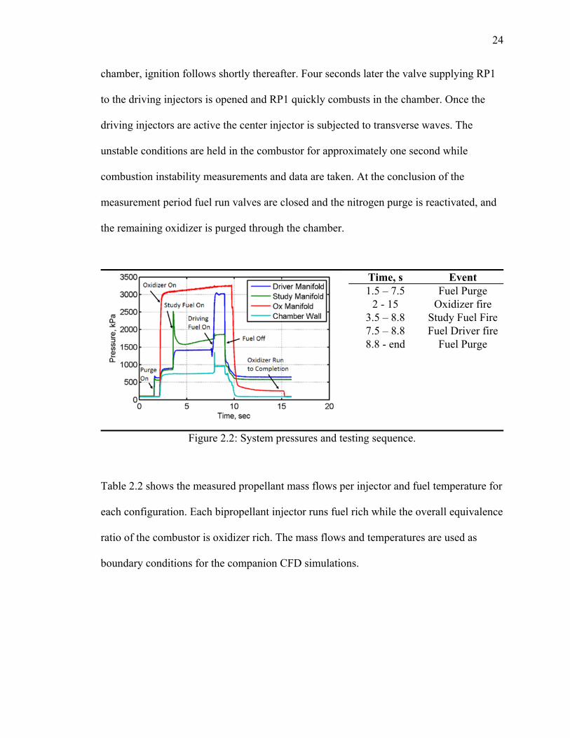
While the primary mode generally contains the most energy, it is also important to

consider the effects of higher order modes as evidenced in Figure 2.7. The figure shows

high-pass filtered pressure at the chamber side wall (shown in black) along with six band-

passed modes centered on the six acoustic frequencies picked up through PSD analysis.

The six band-passed modes were then summed to reveal a form (shown in blue)

representative of the high-pass pressure signal. The peak amplitudes in the high-passed

signal represents the moment the transverse wave impacts the side wall. The strongest

peaks arise as the peaks in the band-passed mode are aligned in phase. It is clear that the

first acoustic mode signal starts rising before the higher order modes. Comparing the

high-pass filtered waveform in the top and bottom figure one can see the rise of

secondary satellite peaks in the first configuration. The secondary peaks appear to be a

consequence of the 4-6th higher order modes aligning. This shows higher order modes

can contribute significantly to waveform shape and is an important fact to consider when

comparing simulations and experiments.

31

Figure 2.7: Band-pass decomposition of high-pass filtered wall pressure for the first configuration (bottom) and second configuration (top).

The amplitude of the pressure wave changes across the chamber, which is

important to know when considering what is affecting the center injector. This change

can be visualized by using four pressure transducer signals that are aligned across the

chamber as shown in Figure 2.8. The line color of each signal corresponds with the port

location color. As the wave moves from the red port to the green port the amplitude is

dampened. This is due to the wave nearing the pressure antinode at the chamber center.

The transverse wave front can also be picked out moving from right to left in the chamber

looking at the pressure signal peaks. At time one the wave front is at the right wall and

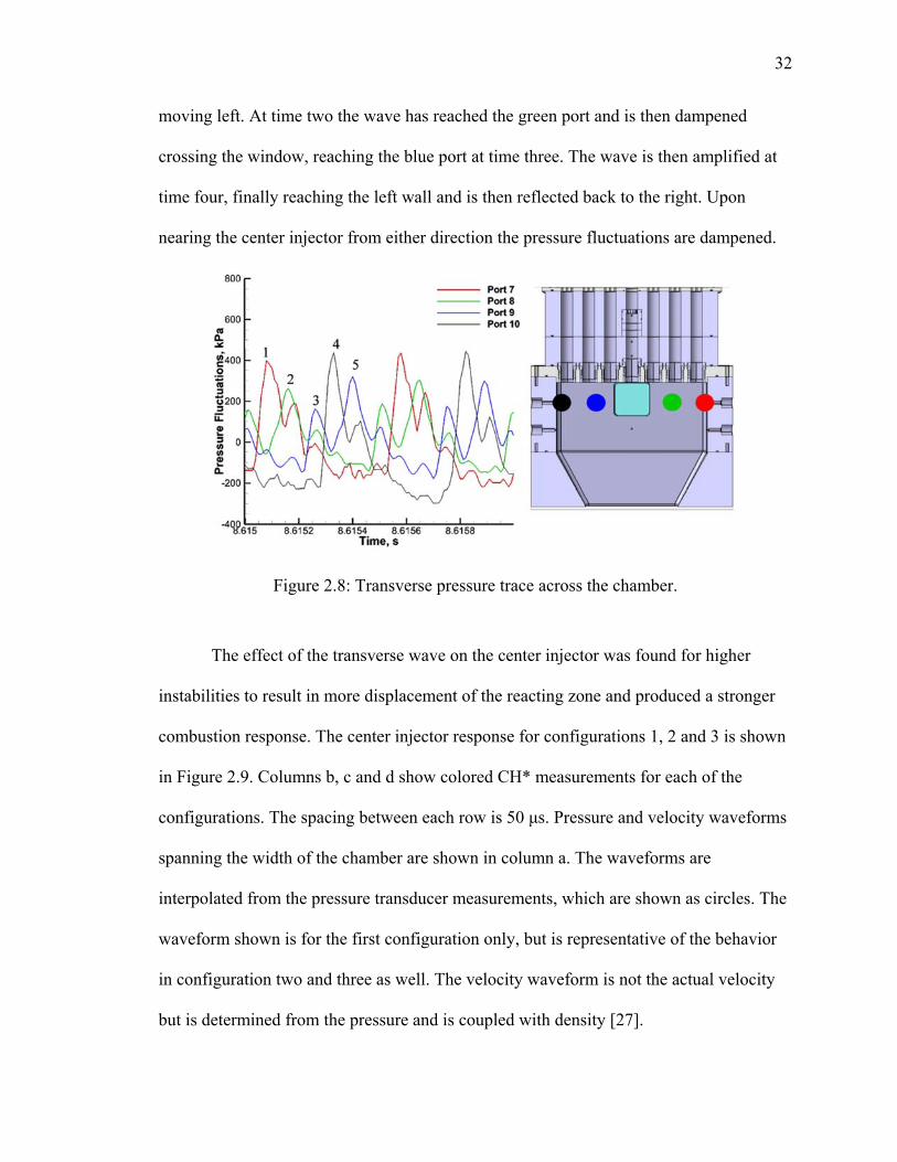
32

moving left. At time two the wave has reached the green port and is then dampened

crossing the window, reaching the blue port at time three. The wave is then amplified at

time four, finally reaching the left wall and is then reflected back to the right. Upon

nearing the center injector from either direction the pressure fluctuations are dampened.

Figure 2.8: Transverse pressure trace across the chamber.

The effect of the transverse wave on the center injector was found for higher

instabilities to result in more displacement of the reacting zone and produced a stronger

combustion response. The center injector response for configurations 1, 2 and 3 is shown

in Figure 2.9. Columns b, c and d show colored CH* measurements for each of the

configurations. The spacing between each row is 50 μs. Pressure and velocity waveforms

spanning the width of the chamber are shown in column a. The waveforms are

interpolated from the pressure transducer measurements, which are shown as circles. The

waveform shown is for the first configuration only, but is representative of the behavior

in configuration two and three as well. The velocity waveform is not the actual velocity

but is determined from the pressure and is coupled with density [27].

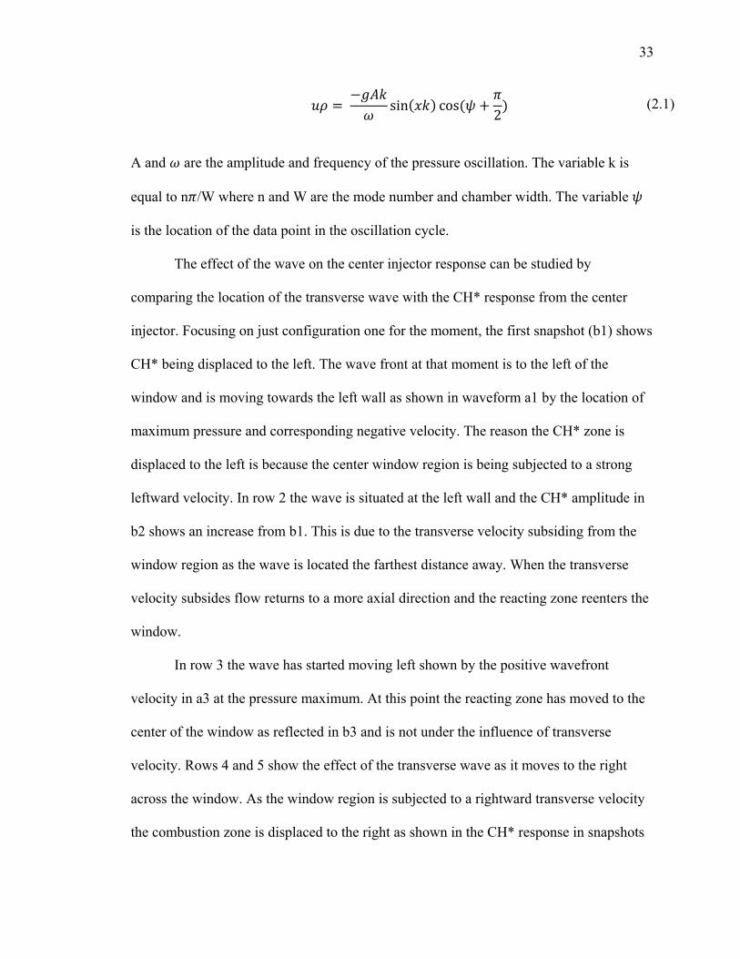
33

sin cos

2 (2.1)

A and are the amplitude and frequency of the pressure oscillation. The variable k is

equal to n /W where n and W are the mode number and chamber width. The variable

is the location of the data point in the oscillation cycle.

The effect of the wave on the center injector response can be studied by

comparing the location of the transverse wave with the CH* response from the center

injector. Focusing on just configuration one for the moment, the first snapshot (b1) shows

CH* being displaced to the left. The wave front at that moment is to the left of the

window and is moving towards the left wall as shown in waveform a1 by the location of

maximum pressure and corresponding negative velocity. The reason the CH* zone is

displaced to the left is because the center window region is being subjected to a strong

leftward velocity. In row 2 the wave is situated at the left wall and the CH* amplitude in

b2 shows an increase from b1. This is due to the transverse velocity subsiding from the

window region as the wave is located the farthest distance away. When the transverse

velocity subsides flow returns to a more axial direction and the reacting zone reenters the

window.

In row 3 the wave has started moving left shown by the positive wavefront

velocity in a3 at the pressure maximum. At this point the reacting zone has moved to the

center of the window as reflected in b3 and is not under the influence of transverse

velocity. Rows 4 and 5 show the effect of the transverse wave as it moves to the right

across the window. As the window region is subjected to a rightward transverse velocity

the combustion zone is displaced to the right as shown in the CH* response in snapshots

34

b4 and b5. Snapshot b5 reflects the effect on CH* when the wavefront is located in the

middle of the chamber. Lastly, in the sixth row, the transverse wave front has moved past

the right window boundary and has imparted a rightward velocity to the reaction zone

region. This causes CH* shown in snapshot b6 to displace further right and extend

beyond the window boundary.

Further comparing CH* measurements between the different configurations in

columns b, c and d shows how the different transverse wave velocity amplitudes affect

the displacement and amount of CH* produced. Comparing column b and column c the

overall displacement of CH* appears very similar, however the amount of CH* which is

shown in greatest concentration by the dark red regions show more in configuration one

(column b) than configuration two (column c). Further looking at the low instability case

(column c) there is very little displacement of CH* but does appear disrupted at the

moments the transverse wave passes the window.

The different configurations show that stronger transverse waves amplify CH*

production and push the reaction zone further beyond the window. The reaction zone also

expands upstream in higher instability configurations which may be due to enhanced

mixing between fuel and oxidizer that is injected from the center study element.

35

Figure 2.9: Center injector response over a half cycle – configuration 1 pressure waveform and transverse velocity (first column). Dots on the plot indicate transducer

measurements and the window lies between the black lines. CH* plots for configuration 1 (second column), 2 (third column), and 3 (fourth column). The time interval between

rows is 50 μs.

36

2.3.1 Dynamic Mode Decomposition

In this section an analysis technique called dynamic mode decomposition is

applied to the CH* measurements from configuration one for later comparison with

simulations. Comparing the CH* images with simulation heat release is difficult because

CH* is a qualitative measurement and the unsteady nature of the flowfield continually

displaces the reacting zone. Prior studies have compared CH* measurements with

simulations using Rayleigh index and time averaging [36], these techniques show similar

behavior in the average sense but do not capture the unsteady behavior.

Modal decomposition is a technique that takes high dimensional flowfields and

breaks them down into fewer degrees of freedom to develop a better understanding of

underlying physical mechanisms. Proper orthogonal decomposition (POD) and dynamic

mode decomposition (DMD) are two types of modal decomposition techniques and have

been applied to study flowfield dynamics [60, 61] and have been growing in the field of

combustion instability [62, 63, 64]. Huang [64] demonstrated the application of POD and

DMD to the reacting flowfield in an unstable longitudinal configuration. The

decomposition was successful in elucidating relationship between pressure and heat

release modes.

POD and DMD each have their own advantages and disadvantages. Both methods

can be used to create a lower-order representation of the flowfield by adding up several

of the dynamic modes. The advantage of DMD over POD is that by basing each dynamic

mode upon a distinct frequency, relationships between variables like pressure, velocity,

and heat release can be compared more directly. Each mode in POD on the other hand is

comprised of multiple frequencies which makes unsteady mode behavior less clear. The

37

advantage of POD over DMD is that it can be applied to any image set while DMD

applies a linear tangential approximation to nonlinear cases which makes it only reliable

during limit cycle of an instability as the event is periodic.

Application of DMD to the CH* measurements in configuration one reveals how

transverse velocity and pressure both affect the spatial location of CH* throughout the

cycle. Modal decomposition was performed on CH* video from configuration one for

100 instability limit cycles. Those results are plotted in Figure 2.10 for half an instability

cycle with the corresponding waveform that shows where the transverse wave is with

respect to the window. Column b shows the DMD of CH* response at the first acoustic

mode and column c shows the DMD of CH* response at the second acoustic mode. Each

row corresponds to the same time that was plotted in Figure 2.9. The two modes

presented have the largest eigenvalues in the system meaning they represent the best two

mode approximation of the flowfield. As a velocity antinode lies at the center of the

window for the first acoustic mode the response of CH* filtered by DMD at that first

acoustic mode can be interpreted as a response to the transverse velocity fluctuations.

And likewise, as a pressure antinode lies at the chamber center for the second acoustic

mode the effect on CH* production for the second DMD mode can be interpreted as a

response to pressure oscillations.

In row one, the transverse wave has just passed the window and is moving left as

shown by the pressure waveform (a1). The first DMD mode in b1 shows that CH*

follows the motion of the transverse velocity to the left with a small zone in the bottom

right convecting downstream. The second mode (c1) shows two small lobes of heat

release moving downstream after the wave has passed. In row two the wave has reached

38

the left wall and CH* has spreads downstream as the transverse velocity subsides and

appears to increase in intensity. The second DMD acoustic mode (c2) shows CH* being

produced in the center of the window, upstream and between the two heat release lobes as

pressure decreases in the chamber center. In the third row the transverse velocity has

decreased even further and CH* (b3) continues to move further downstream. The second

mode shows a strong increase in CH* (c3) which is close to a pressure minimum in the

cycle and may be due to an expansion of oxidizer into the fuel.

The next three rows show the effect of the return of the transverse wave. In row

four the transverse velocity has picked up and is moving rightward as the wave

approaches the left side of the window. CH* formation is interrupted in the first DMD

mode (b4) and begins to move to the right. In the second mode, CH* decreases (c4) as

pressure begins to rise. Then in row five the transverse velocity is nearing a maximum

and complete disruption of CH* is evident in the first mode (b5) as a reaction zone shifts

from the left side of the window to the right. The second mode (c5) shows further CH*

disruption as the second mode pressure increases in the chamber center, also nearing a

maximum. And lastly in row six the transverse wave has completely crossed the window

and the reaction zone in mode 1 (b6) has completely moved to the right side of the

window and spreads further downstream. The second DMD mode shows two remaining

CH* lobes just like the first row with pressure near a maximum.

What is learned from the modal decomposition is that the transverse wave

interrupts CH* formation as it passes the window. As the wave moves beyond the

window a higher concentration of CH* is seen. This implies an oscillating cycle of

increasing and then decreasing heat release in response to the wave.

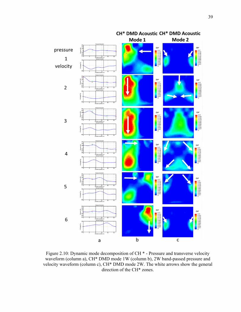
39

Figure 2.10: Dynamic mode decomposition of CH * - Pressure and transverse velocity waveform (column a), CH* DMD mode 1W (column b), 2W band-passed pressure and

velocity waveform (column c), CH* DMD mode 2W. The white arrows show the general direction of the CH* zones.

40

In this chapter, the setup for both the second and third generation TIC was

presented. The propellant type, mass flows and fuel temperature are later used for direct

input into the simulation boundary condition and initial conditions. High frequency

pressure and optical CH* measurements are taken to understand how the combustor

responds. Results were shown from the second generation experiment. The purpose was

to provide a better understanding of how the different instability configurations affect the

pressure fluctuations in the combustor and the subsequent effect on the center injector

response as those results are used for later comparison with simulations.

It was found that the first mode played a dominant role in the higher instability

configurations and higher modes also became significant when looking at the pressure

waveform. Under the different configurations the CH* response from the center injector

was found to grow under stronger instabilities and transverse displacement from the

center axis was also found to increase. Further analysis applying DMD showed that when

the transverse wave hits center injector the combustion process is interrupted and as the

wave moves towards the side walls heat release in the first and seconds modes grows. As

the results are for only two modes a global interruption of heat release cannot be assumed

but the results do imply a decrease in heat release as the wave passes.

41

CHAPTER 3. MODELING APPROACH

A primary objective of this work is to explore the predictive capabilities of high-fidelity

computational fluid dynamics simulations. GEMS, the general equation and mesh solver,

is an in house CFD code developed at Purdue [65- 68], and is employed in this study.

GEMS can be used to simulate unsteady reacting flows which is a requirement of

instability modeling. To simulate the transverse instability chamber that was described in

the previous chapter, two distinct approaches are used. The first approach is focused on

studying the response of the central injector element to high amplitude transverse

acoustics oscillation. For this study, only three of the seven injectors are modeled; the

remaining two driving injectors on each side are omitted. The transverse oscillation is

generated by vibrating the side walls, which represents the net effect of the outside

driving elements as explained in detail later in this chapter. The second approach is used

to study the mechanisms underlying the generation of the transverse oscillations and

require that all seven injectors are modeled. Although more expensive, this level of

modeling is necessary to fully capture the self-excited nature of the instability. Moreover,

the full-seven injector model can also be used to study element to element reactions.

This chapter is organized into three sections. The first section describes the

modeling approach in GEMS with details provided about turbulence modeling and

reaction kinetics. The remaining two sections detail the setup of the three- and seven-

42

injector modes. For each approach the computational mesh, boundary conditions, initial

conditions, and reaction models are described.

3.1 Computational Solver

GEMS is a second-order implicit finite-volume code. It numerically solves the

Navier-Stokes equations, comprised of the continuity, momentum, energy, turbulence

and coupled species equations. A source term is introduced in the species conservation

equations for species production and consumption. A dual-time iterative procedure is

used to eliminate linearization and approximate factorization errors. The conservation

equations can be expressed compactly in vector form,

∙ (3.1)

where Q is the vector of conserved variables, defined as,

ℓ (3.2)

where is density, is the velocity in the x, y and z directions, is stagnation enthalpy,

p is the pressure, and ℓ is species mass fraction of species ℓ. The flux vectors are , and

which represent the inviscid and viscous components respectively. Each flux can be

further decomposed into components in the x, y, and z directions:

(3.3) (3.4)

The three inviscid flux vectors from equation 3.3 are,

43

ℓ ℓ

ℓ

(3.5)

and the viscous flux vectors are,

,

0

,ℓ ℓ

(3.6)

where we have omitted the turbulence transport equations, which are discussed later.

Several additional terms are introduced in the viscous fluxes, including the shear

stress, heat flux, qi and diffusion velocity, Vi,ℓ. The shear stress is defined in terms of

the viscosity, μ, and the gradient of the velocity field.

23

(3.7)

The heat flux is defined as the heat transfer due to conduction, species diffusion, and heat

generation from a volumetric heat source:

,ℓ

ℓ

ℓ ℓ (3.8)

,

0

,ℓ ℓ

,

0

,ℓ ℓ

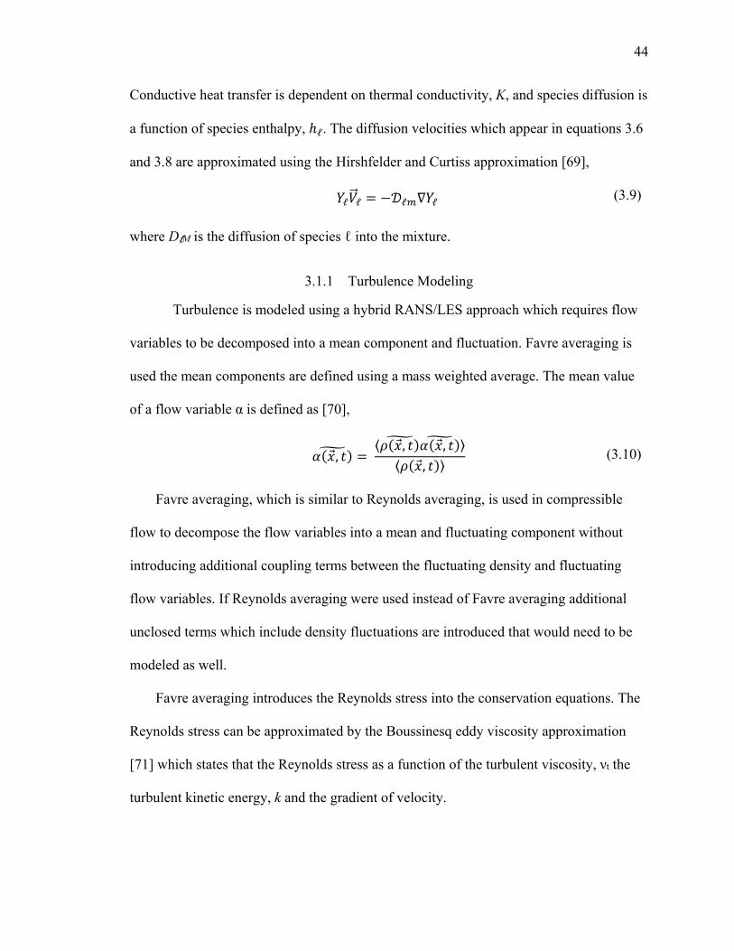
44

Conductive heat transfer is dependent on thermal conductivity, K, and species diffusion is

a function of species enthalpy, ℓ. The diffusion velocities which appear in equations 3.6

and 3.8 are approximated using the Hirshfelder and Curtiss approximation [69],

ℓ ℓ ℓ ℓ (3.9)

where DℓM is the diffusion of species ℓ into the mixture.

3.1.1 Turbulence Modeling

Turbulence is modeled using a hybrid RANS/LES approach which requires flow

variables to be decomposed into a mean component and fluctuation. Favre averaging is

used the mean components are defined using a mass weighted average. The mean value

of a flow variable α is defined as [70],

,

⟨ , , ⟩⟨ , ⟩

(3.10)

Favre averaging, which is similar to Reynolds averaging, is used in compressible

flow to decompose the flow variables into a mean and fluctuating component without

introducing additional coupling terms between the fluctuating density and fluctuating

flow variables. If Reynolds averaging were used instead of Favre averaging additional

unclosed terms which include density fluctuations are introduced that would need to be

modeled as well.

Favre averaging introduces the Reynolds stress into the conservation equations. The

Reynolds stress can be approximated by the Boussinesq eddy viscosity approximation

[71] which states that the Reynolds stress as a function of the turbulent viscosity, νt the

turbulent kinetic energy, k and the gradient of velocity.

45

23

23

(3.11)

Additional unclosed terms similar to the Reynolds stress can be found in the energy

and species equations. These terms are closed using the gradient diffusion hypothesis and

either a turbulent Prandtl number in the case of the energy equation or turbulent Schmidt

number for the species equations. The turbulent Prandtl number and turbulent Schmidt

number are taken to be constant, with values of 0.71 and 0.9 respectively. For the present

work the two-equation k-ω turbulence model is used [72]. The model introduces two new

conservation equations, one for the turbulent kinetic energy (k) and one for the specific

dissipation (ω). The conservation equations are,

⟨ ⟩⟨ ⟩ ⟨ ⟩ ⋆ ⋆

⟨ ⟩ (3.12)

⟨ ⟩⟨ ⟩

⟨ ⟩⟨ ⟩ ⟨ ⟩

⟨ ⟩ (3.13)

The parameters ⋆, ⋆, , , , and are closure constants specified in the k-ω

model [72]. To determine the Reynolds stress the turbulent viscosity is needed, and is

defined as,

ω

(3.14)

where ω is the shear stress limited specific dissipation, a function of ω, and the strain rate

tensor. Turbulence is modeled using a hybrid RANS/LES approach [73, 74]. To

46

implement the hybrid model a turbulent length scale is required, in the k-ω model it is

defined as,

/

⋆ (3.15)

The turbulent length scale is a part of the second term on the right hand side of equation

3.12 and arises as follows:

⋆ /

When grid size is small enough to resolve the turbulent length scale that grid size is set as

the turbulent length allowing for resolution of the large eddies in the simulation. If

smaller, the length scale is computed from equation 3.15 and turbulence is solely

modeled without resolving eddies.

3.1.2 Reacting Flow

For reacting flow a source term is present in equation 3.1, and represents the production

or consumption of species due to reactions,

0 0 0 0 0 ℓ (3.16)

The species production term is determined by the summation of the rate of progress

variable ( ) for each reaction. The summation is made over M reaction equations for

species, ℓ [75].

ℓ ℓ ℓ ℓ (3.17)

where ℓ and ℓ are the stoichiometric coeffiencents of the products and reactants

respectively. ℓ is the molecular weight of the ℓth species. The rate of progress variable

47

is determined from the forward and reverse reaction rates, and species molar

concentrations ([Xℓ]) where N is the total number of species.

, ℓ

ℓ

ℓ

, ℓℓ

ℓ

(3.18)

The simulations in this thesis model species production only in terms of the forward

reaction rate, which is given in the Arrhenius form,

(3.19)

The reaction takes place once the activation energy Ea is reached. The pre-exponential

factor A, parameter b, and activation energy are calculated from detailed chemical

kinetics attempting to match certain experimental data like flame speed or ignition delay

time. [76].

Once the species production is calculated, heat release produced from combustion

is determined knowing the enthalpy of formation of the species, Δ ,ℓ .

Δ ,ℓ ℓ

ℓ

(3.20)

The flame produced is only a function of mean quantities and is thus a laminar flame rate

model. All species are modeled using an ideal gas equation of state and the

thermodynamic and transport properties are evaluated through polynomial fit data. A

more detailed description of GEMS is provided elsewhere [11].

48

3.1.3 Data Output

Data in the simulations is collected in three different formats using techniques

developed by Smith and Harvazinski [11, 32]. A point monitor is used to output detailed

data with a high temporal resolution at specified locations. This is similar to experimental

pressure transducers and thermocouples. The full three-dimensional flowfield is also

output at specified intervals; these files hold all variable information throughout the

calculation. The plots can be used to look at heat release control contours for comparison

with the experiments and for exploring the physical processes occurring in the flowfield.

Lastly, variable data is output in volume integrals. Here, specified quantities are spatially

integrated over a specified volume. The volume integral data allow for faster processing

than the instantaneous flowfield plots and are used to analyze the flowfield solution in

specific regions of interest. On the other hand, point monitor and volume integral

measurements are relatively inexpensive in terms of file size compared to the

instantaneous flowfield.

3.2 Three Injector Setup

This section provides details of the three-injector model setup. First the

computational domain is presented along with information about the computational mesh.

Then a description of the boundary conditions and initial conditions is given. The

velocity forcing function employed at the side-walls to mimic the experimental instability

amplitude is described. Finally, the reaction kinetics models used in the simulations are

also presented.

49

3.2.1 Geometry and Grid Generation

The three injector setup serves as a model of the second generation experiment. The

computational domain is shown in Figure 3.1. The dimensions match those of the

experiment excluding the geometry of the outer four injectors, which are not modeled

(since the focus of this configuration is on analyzing the response of the center injector).

The simulations are setup to match the experimental configurations shown in Table 2.1.

The choke plate for the two outer injectors in the experiment is not modeled in the

simulation due to the onerous mesh requirements; however the individual choke plate in

the center injector is still modeled in order to capture the vortical structures downstream

of the choke plate. At the base of the center injector, gaseous ethane fuel is injected

through an annulus around the central oxidizer core. Both the choke plate and fuel

annulus cross sections are shown in Figure 3.1. A slight expansion is added downstream

of the nozzle throat with a six-degree half angle. This is not part of the experimental

geometry but is added in the simulation so that a uniform back-pressure can be applied at

an appropriate location.

50

Figure 3.1: Computational domain for the simulation and grid mesh.

Meshing the geometry is always a major task in CFD modeling and the ultimate goal

is to reach a grid-independent solution. The mesh that we have designed for this

geometry is relatively coarse, consisting of 2.7 million nodes and is block structured.

Higher resolution grids are more costly in terms of computational time and power

requirements and so must be weighed against the available resources. Resolving the wall

boundary layer is a major source of the number of grid points. This is because a large

number of grid points lie in the boundary layer to capture the gradients between the outer

turbulent layer and viscous sub-layer near the wall. Required boundary layer resolution is

dependent on the turbulence model used [77] and is measured by the y+ value which is

the non-dimensional distance from the wall to the first grid point. The two-equation k-ω

turbulence model used in these simulations requires a y+ value of unity to properly

51

capture the viscous sub-layer to enforce the no-slip condition. y+ values of unity are

achieved in the main combustor and nozzle. However it was not possible to do so within

the choke plate slots and the main fuel injector since the introduction of the additional

grid points would need to be carried downstream throughout the entire chamber, greatly

impacting the total mesh size. Figure 3.2 shows a representative mesh used in the current

study.

Figure 3.2: Three injector model mesh.

To create the structured mesh a block is first placed around the combustor geometry.

This initial block is then subdivided into smaller blocks until each geometric feature is

represented by a single block. O-grids are then specified for each injector which is

required to mesh the circular tubes. An additional o-grid is specified from all the inlets to

outlets to create the boundary layer mesh. Once blocking is completed all of the edge

52

parameters are set to place the edge nodes. As mentioned the grid points are densely

packed in the boundary layer and in regions of interest like the injection region.

Mesh quality is very important for convergence and small mesh errors can lead to a

solution, which may not converge. Moreover, the quality of the mesh needed to reach a

converged solution is dependent on the solver and is problem specific. Several metrics

can be used to analyze the mesh quality including the cell determinant, cell aspect ratio

and cell angle. The determinant is checked to make sure the cell has positive orientation

(volume). The determinant is also a measure of the cell’s shape. The closer it is to unity

the closer it is to a perfect cube. If the determinant is negative then the cell is inverted

(faces intersect) and the mesh needs to be corrected. Generally, a mesh is designed to

have a determinant > 0.3. Cell aspect ratio is another important parameter that needs to be

checked and is especially important near the wall where the aspect ratio can grow very

large due to the small spacing between the wall and first grid point. The aspect ratio is

generally kept at a value less than 1000. There is always a balancing act between the y+

values and aspect ratio. The only way to decrease the aspect ratio for a certain y+ value is

to add more grid points along the wall, which again increases computational time. The

cell angle is another parameter that needs to be checked and as a rule of thumb is kept

greater than 30 degrees. The ideal cell is a cube with a 90 degree angle. The mesh quality

of the three injector mesh is presented in Table 3.1. It should be noted that in geometries

with circular cross sections, like those present in the TIC, the maximum angle achievable

is 45 degrees.

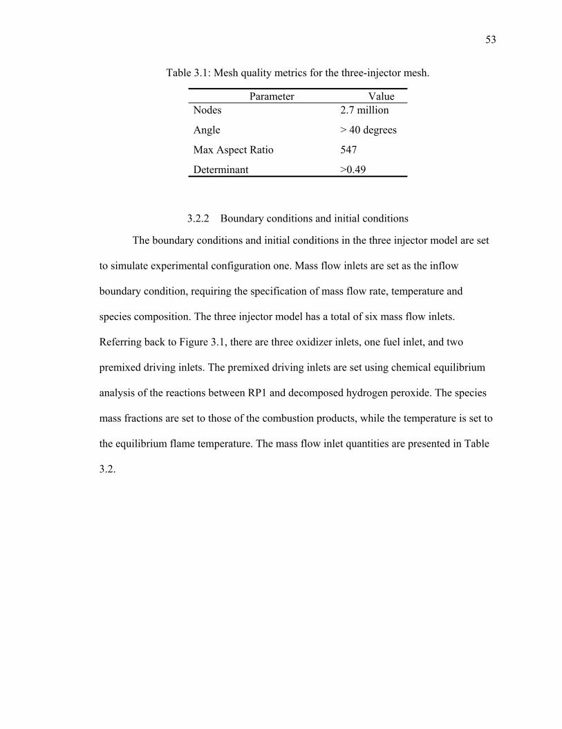
53

Table 3.1: Mesh quality metrics for the three-injector mesh.

Parameter Value Nodes 2.7 million

Angle > 40 degrees

Max Aspect Ratio 547

Determinant >0.49

3.2.2 Boundary conditions and initial conditions

The boundary conditions and initial conditions in the three injector model are set

to simulate experimental configuration one. Mass flow inlets are set as the inflow

boundary condition, requiring the specification of mass flow rate, temperature and

species composition. The three injector model has a total of six mass flow inlets.

Referring back to Figure 3.1, there are three oxidizer inlets, one fuel inlet, and two

premixed driving inlets. The premixed driving inlets are set using chemical equilibrium

analysis of the reactions between RP1 and decomposed hydrogen peroxide. The species

mass fractions are set to those of the combustion products, while the temperature is set to

the equilibrium flame temperature. The mass flow inlet quantities are presented in Table

3.2.

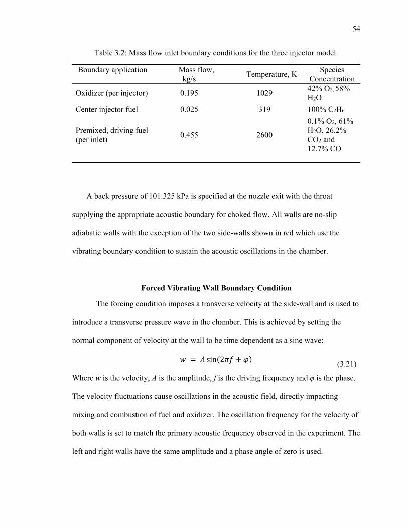
54

Table 3.2: Mass flow inlet boundary conditions for the three injector model.

Boundary application Mass flow, kg/s

Temperature, K Species

Concentration

Oxidizer (per injector) 0.195 1029 42% O2, 58% H2O

Center injector fuel 0.025 319 100% C2H6

Premixed, driving fuel (per inlet)

0.455 2600

0.1% O2, 61% H2O, 26.2% CO2 and 12.7% CO

A back pressure of 101.325 kPa is specified at the nozzle exit with the throat

supplying the appropriate acoustic boundary for choked flow. All walls are no-slip

adiabatic walls with the exception of the two side-walls shown in red which use the

vibrating boundary condition to sustain the acoustic oscillations in the chamber.

Forced Vibrating Wall Boundary Condition

The forcing condition imposes a transverse velocity at the side-wall and is used to

introduce a transverse pressure wave in the chamber. This is achieved by setting the

normal component of velocity at the wall to be time dependent as a sine wave:

sin 2 (3.21)

Where w is the velocity, A is the amplitude, f is the driving frequency and φ is the phase.

The velocity fluctuations cause oscillations in the acoustic field, directly impacting

mixing and combustion of fuel and oxidizer. The oscillation frequency for the velocity of

both walls is set to match the primary acoustic frequency observed in the experiment. The

left and right walls have the same amplitude and a phase angle of zero is used.

55

When superimposed the two waves create a standing wave. Figure 3.3 shows the

pressure and velocity mode shapes in the three-injector model generated by vibrating the

walls on the left and right of the chamber. The mode shapes are a one-dimensional

representation of pressure and velocity across the combustor. Pressure and velocity have

been spatially averaged as well as phase averaged to create the plots shown. They

indicate that there are large pressure fluctuations at the side walls as opposed to the

central region, where a pressure node exits for the first mode. The center injector lies at

this pressure node, which also is a velocity antinode, and this injector is therefore

subjected to strong velocity oscillations. Placing the center injector at this location allows

for studying velocity oscillation effects on the reaction zone downstream of the center

injector.

Figure 3.3: Primary velocity (left) and pressure (right) mode shapes in the three injector simulation.

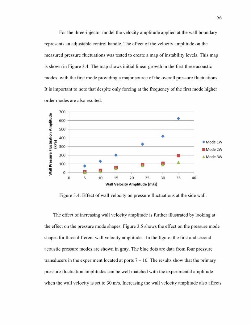
56

For the three-injector model the velocity amplitude applied at the wall boundary

represents an adjustable control handle. The effect of the velocity amplitude on the

measured pressure fluctuations was tested to create a map of instability levels. This map

is shown in Figure 3.4. The map shows initial linear growth in the first three acoustic

modes, with the first mode providing a major source of the overall pressure fluctuations.

It is important to note that despite only forcing at the frequency of the first mode higher

order modes are also excited.

Figure 3.4: Effect of wall velocity on pressure fluctuations at the side wall.

The effect of increasing wall velocity amplitude is further illustrated by looking at

the effect on the pressure mode shapes. Figure 3.5 shows the effect on the pressure mode

shapes for three different wall velocity amplitudes. In the figure, the first and second

acoustic pressure modes are shown in gray. The blue dots are data from four pressure

transducers in the experiment located at ports 7 – 10. The results show that the primary

pressure fluctuation amplitudes can be well matched with the experimental amplitude

when the wall velocity is set to 30 m/s. Increasing the wall velocity amplitude also affects

57

the higher harmonic modes as seen by the amplitude increase in the pressure mode shape

filtered at the 2nd mode. While there is discrepancy between the experiment and

simulation second mode amplitude, this approach provides a good first-order

approximation of matching instability levels observed in the experiment. Better matches

of all the modal amplitudes may be achieved by superimposing multi-frequency wall

velocity oscillations.

Figure 3.5: Pressure mode shapes for the 1st (left column) and 2nd (right column) modes. Each row represents a different wall velocity boundary condition: 23.5m/s (top), 30 m/s

(middle), 35 m/s (bottom), experimental data from port 7 – 10 is overlaid in blue.

58

The initial pressure throughout the domain is set to the mean chamber pressure in the

experiment during unstable operation: 965 kPa in this case. The oxidizer tubes are filled

with 42% O2 and 58% H2O each at 1029K and the center fuel annulus is filled with

ethane at 319 K. The side driving injector inlet volumes are filled with the same species

mass fractions as their boundary conditions at 2600K. The chamber is initially filled with

reacted species products – 70% H2O and 30% CO2 at 800K. The model is initially run

without the vibrating wall activated, once the initial transient is washed out, the vibrating

wall is activated.

3.2.3 Reaction Kinetics

Combustion in the three-injector simulations as well as seven-injector simulations

presented later is modeled using global reactions. Global reactions allow coupling of

unsteady heat release and pressure to be captured while minimizing the number of

species that must be included. Global or reduced order kinetics models are needed when

running high fidelity three dimension CFD simulations because of the expensive cost of

including large numbers of species. Using a detailed reaction mechanism would greatly

add to the computational cost.

The focus of the three-injector simulations is on the combustion response of the

center study element, which involves the reaction is between the ethane fuel and the

oxygen from the decomposed hydrogen peroxide. A two-step global reaction model was

chosen for ethane combustion that incorporates five species: C2H6, O2, H2O, CO2, and

CO. The first reaction and second reaction are shown below. The first reaction involves

the combustion of ethane with oxygen which forms the species products H2O and CO.

The second equation is a reversible reaction involving CO, O2, and CO2.

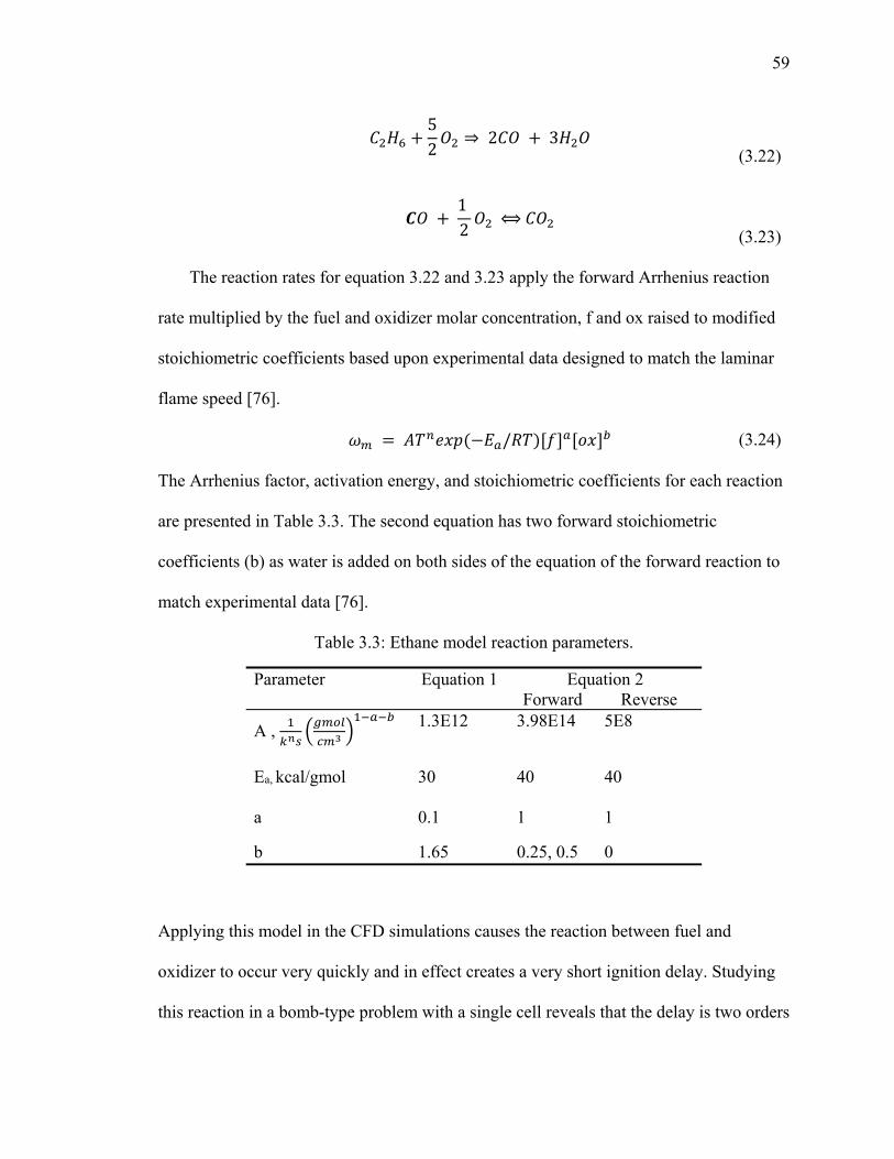
59

52

⇒ 2 3 (3.22)

12

⟺ (3.23)

The reaction rates for equation 3.22 and 3.23 apply the forward Arrhenius reaction

rate multiplied by the fuel and oxidizer molar concentration, f and ox raised to modified

stoichiometric coefficients based upon experimental data designed to match the laminar

flame speed [76].

/ (3.24)

The Arrhenius factor, activation energy, and stoichiometric coefficients for each reaction

are presented in Table 3.3. The second equation has two forward stoichiometric

coefficients (b) as water is added on both sides of the equation of the forward reaction to

match experimental data [76].

Table 3.3: Ethane model reaction parameters.

Parameter

Equation 1 Equation 2 Forward Reverse

A ,

1.3E12 3.98E14 5E8

Ea, kcal/gmol

30 40 40

a 0.1 1 1

b 1.65 0.25, 0.5 0

Applying this model in the CFD simulations causes the reaction between fuel and

oxidizer to occur very quickly and in effect creates a very short ignition delay. Studying

this reaction in a bomb-type problem with a single cell reveals that the delay is two orders

60

of magnitude faster than that seen in experiments [78] as shown in Figure 3.6. The

simulation data for the reaction bomb problem is plotted in green as compared to the

experimental data shown in red at two different pressure levels. By decreasing the

Arrhenius factor by two orders of magnitude it was found that the ignition delay in the

bomb problem (shown in blue) more closely matches that observed in the experiment

[78]. Inputting this modified Arrhenius factor into the reaction model was then tested in

the three injector simulations to evaluate the instability performance, described in the

next chapter.

Figure 3.6: Ignition delay comparison between simulations with the original Arrhenius factor (green), modified Arrhenius factor (blue) and experimental data (red) [78].

3.3 Seven Injector Setup

This section provides the details of the seven injector model setup, including the

expanded mesh and details about the boundary conditions and initial conditions. Unlike

the three-injector simulation, a velocity forcing function is not employed in the full

geometry simulations as the actual mechanisms driving the flow behavior in the

experiment are of interest.

61

3.3.1 Geometry and Grid Generation

The seven-injector model geometry is presented in Figure 3.7. The geometry is

modeled after the third generation experiment, which is similar to the second generation

combustor. There are a few small differences in chamber length and nozzle size as well

as the injector vortex chamber length but the combustor for the most part is very similar

with the same chamber width and oxidizer post lengths as its predecessor. The same

oxidizer, decomposed hydrogen peroxide is used and the fuel is gaseous methane.

In the experiment the oxidizer is choked with nozzles at the inlets of the outer six

injectors and the same choke plate is used in the center injector as in the previous

experiment. At this stage the nozzle inlet geometry has not been applied to the simulation

but will be considered in future models. Fuel is no longer swirled in the experiment outer

injectors which will provide a better comparison with simulation results. The same fuel

annulus configuration applied in the three injector model is used in the seven injector

model as shown in slice B with fuel injected parallel to the oxidizer flow. Methane fuel is

only flown in the center and outer four fuel injectors to match the same configuration of

the three injector model and prior experiment.

62

Figure 3.7: Seven injector model geometry.

The mesh of this geometry is presented in Figure 3.8 and is designed similarly to

the three injector mesh; however the addition of the outer injectors and further grid

continued refinement increased the number of cells from 2.7 million to 12.5 million. For

instance, finer wall distances are included in the boundary layer, which require more grid

points to decrease the aspect ratio of the cells.

The y+ values are unity in the main chamber flow but again are larger in the fuel

injectors due to the impact decreasing the y+ values would have on the total number of

grid points. The overall quality metrics are similar to the three injector grid and are

summarized in Table 3.4. The aspect ratio is larger than in the previous models.

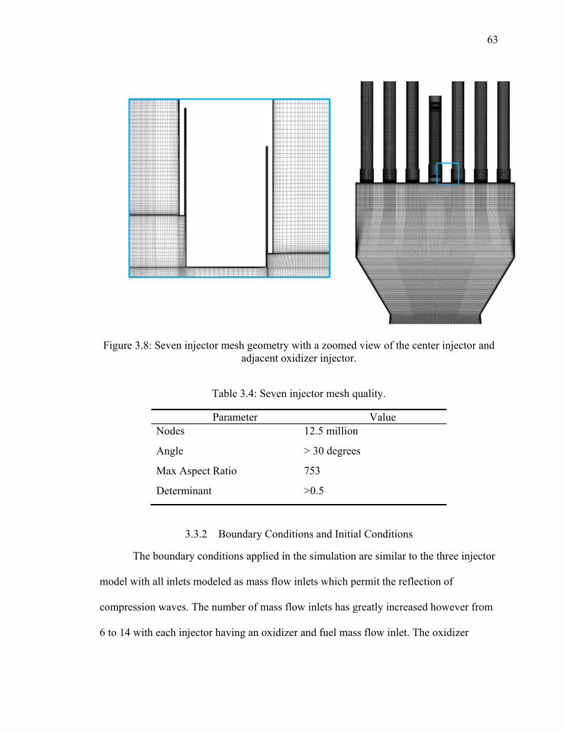
63

Figure 3.8: Seven injector mesh geometry with a zoomed view of the center injector and adjacent oxidizer injector.

Table 3.4: Seven injector mesh quality.

Parameter Value Nodes 12.5 million

Angle > 30 degrees

Max Aspect Ratio 753

Determinant >0.5

3.3.2 Boundary Conditions and Initial Conditions

The boundary conditions applied in the simulation are similar to the three injector

model with all inlets modeled as mass flow inlets which permit the reflection of

compression waves. The number of mass flow inlets has greatly increased however from

6 to 14 with each injector having an oxidizer and fuel mass flow inlet. The oxidizer

64

boundary condition remains the same and new fuel boundary conditions are applied.

Those boundary conditions are shown in Table 3.5. The fuel injectors adjacent to the

center injector are set to flow a very small amount of 42% O2 and 58% H2O because in

the experiment, fuel is not flown through these injectors.

Table 3.5: Mass flow inlet boundary conditions for the seven injector model.

Boundary application Mass flow, kg/s

Temperature, K Species

Concentration Oxidizer (per injector) 0.195 1029 42% O2, 58%

H2O Center injector fuel 0.025 298 100% CH4

Driving fuel (per injector)

0.0329 298 100% CH4

Downstream of the combustor throat the backpressure is set to ambient pressure

with the same six degree half-angle nozzle expansion to ensure that the flow is choked at

the throat. All walls are no-slip adiabatic walls. The initial condition in the chamber is

adjusted to more closely resemble the conditions in the experiment. The geometry is

initially filled with decomposed hydrogen peroxide (42% O2 and 58% H2O) at 1500K in

the combustion chamber and 1029K everywhere else. The initially warm temperature in

the chamber insures that the methane fuel will ignite upon mixing with the oxidizer. It

should also be noted that attempts to run the simulations with an initial temperature of

1029K did not result in ignition.

65

3.3.3 Reaction kinetics

Flowing methane fuel in the central and outer injectors allows for the use of a

simple reaction mechanism in the seven-injector simulations. Specifically, a single-step

global methane reaction is applied that incorporates the four species: CH4, O2, H2O, and

CO2. The reaction is shown in equation 3.25 and the species production is determined

from the parameters presented in Table 3.6. The parameters are again based on

experimental data to match the laminar flame speed [76].

CH 2O → CO 2H O (3.25)

Table 3.6: Single Step Methane Reaction Parameters.

Parameter Equation 1

A ,

6.7E12

EA, kcal/gmol

48.4

a 0.2

b 1.3

66

CHAPTER 4. COMPUTATIONAL ANALYSIS OF INJECTOR RESPONSE

The TIC configuration provides a useful means for testing the response of an injector

element subjected to high amplitude transverse acoustics oscillations. A primary

objective of the current study is to investigate the application of a reduced three-injector

model as a computational test bed for evaluating the injector response to transverse

instability. In other words, the study element is selected to be the central element and

only the two elements on either side are modeled. The acoustic field itself is generated by

forcibly oscillating the side-walls in a manner that matches the TIC acoustic mode

amplitudes. The outcome of the study demonstrates that model is indeed able to capture

the response of the experimental injector and further proves the potential for using high

fidelity CFD simulations to characterize injector stability.

This chapter is divided into four sections. In the first section the initial transient

startup process of the three injector model is presented, followed by a full instability

cycle. A second study looking at the influence of applying different forcing amplitudes is

presented next. A comparison between the simulation results and experiment is also

provided along with analysis which helps to improve the understanding of the injector

response in the experiment.

67

4.1 Startup

The computations are initialized by filling hot combustion products in the chamber.

At time t=0, the oxidizer and fuel start flowing into the domain through the injector

inlets. Initially, the side walls are kept stationary (i.e. no forcing). Ignition occurs after

approximately 100 μs. The initial transient displays stable combustion, and the

combustion remains stable until external forcing is supplied. The ignition process is

shown in Figure 4.1. Ethane fuel, injected in the center study element, reacts with the

central oxidizer core almost immediately and burns inside the injector. The ignition spike

produces waves that reflect off the chamber and side walls, setting up a short duration

second transverse mode which quickly dies down over several milliseconds. The elevated

regions of heat release on the edges of the oxidizer injectors are the result of the

equilibrium reaction between CO2, CO, and O2 as the newly flowing oxidizer mixes with

the background flow.

Figure 4.1: Ignition in the three injector simulation showing reactions from the central study injector and between the bypass flow and side oxidizer streams. The experiment

window size is plotted in white.

68

Initially the simulation is run for 4 ms, allowing the main chamber to fill with fuel

and oxidizer as shown in Figure 4.2. The ethane fuel, injected through the center study

element, is quickly burned in the oxidizer rich environment and is fully consumed by the

midpoint of main chamber. The majority of combustion occurs due to ethane and oxygen

associated with the center injector. A large temperature gradient exists between the hot

bypass flow and oxidizer jet as the combustion products attain the 2600k equilibrium

temperature.

Following the ignition spike, the chamber pressure reaches a stationary value of

1.1 MPa. The manifold upstream of the choke plate has a pressure about three times the

chamber pressure. Note that the choke plate is a source of vorticity generation. As the

oxidizer expands into the oxidizer post vortices are produced, which are then convected

through the oxidizer post into the main chamber. These vortices enhance mixing between

the ethane and oxidizer. The oxidizer-only injectors which sit on either side of the study

element do not have a choke plate, and therefore only a relatively small amount of

vorticity, produced from the interaction with the flow and wall, is observed.

69

Figure 4.2: Unforced flowfield conditions in the three injector simulations of ethane fuel, oxygen and heat release (top row) with zoomed in views (second row). Pressure,

temperature and vorticity are shown in a full view (third row) and near the injection plane (fourth row).

70

Following the initial 4 ms, the walls are set to vibrate which simulates the unstable

behavior that would take place if the driving injectors had been included. The amplitude

of the oscillating wall controls the observed transverse pressure oscillations in the

chamber. Figure 4.3 shows the pressure amplitude for three different forcing amplitudes.

Applying forcing boundary conditions with amplitudes ranging from 5 – 35 m/s produces

instability levels that ranged from 8% to 70% of the mean chamber pressure, covering the

experimental operating range. The pressure fluctuations in the chamber grow to a limit

cycle almost immediately. Following the initial transient the simulation are run for 45 ms

to produce sufficient unsteady data for analysis.

Figure 4.3: Growth to limit cycle for different wall velocity boundary conditions in the three injector simulations. The measurement point is taken at the combustor side wall.

4.2 Instability Cycle

Forcing the side wall sets up a standing transverse wave in the combustion

chamber. This setup is used to understand the response of the center injector to transverse

oscillations. A full instability cycle for the 30 m/s forcing amplitude is shown in Figure

4.4. The wall is forced at a frequency of 2035 Hz. The transverse wave, starting in the left

71

column, moves from left to right across the chamber. As the wave moves across the

chamber, compression waves also move upstream into the injectors. The longitudinal

waves in the injectors are then reflected and travel back into the chamber.

The wave traverse is also influenced by the local speed of sound in the combustor

which changes with temperature. The temperature profile in the chamber is also shown

and over the course of a cycle changes minimally. The region near the injector face is

cooler and thus has a lower sound speed and helps give rise to the resulting wave shape.

The transverse pressure wave is not parallel to the side wall but is instead angled with the

leading edge lying in the converging section of the chamber. This is due to the shorter

travel distance in the converging section of the chamber wall and the locally higher

temperature in the region.

Combustion heat release is also influenced by the transverse wave. As the wave

passes through the center injector propellant stream an elongation of heat release occurs

in the transverse direction near the injection plane, indicated by the white ovals. An

additional heat release zone lies downstream of the center injector near the walls normal

to the plane of view that is not displaced, pointed to by the white arrows. The different

motions between the zones may be caused by the local fuel and oxidizer concentrations in

those regions. The difference in response to the transverse wave in those two zones is

important because it shows that the heat release response is not simply 2D in this

geometry and that fact needs to be considered in how heat release is compared with

experiments.

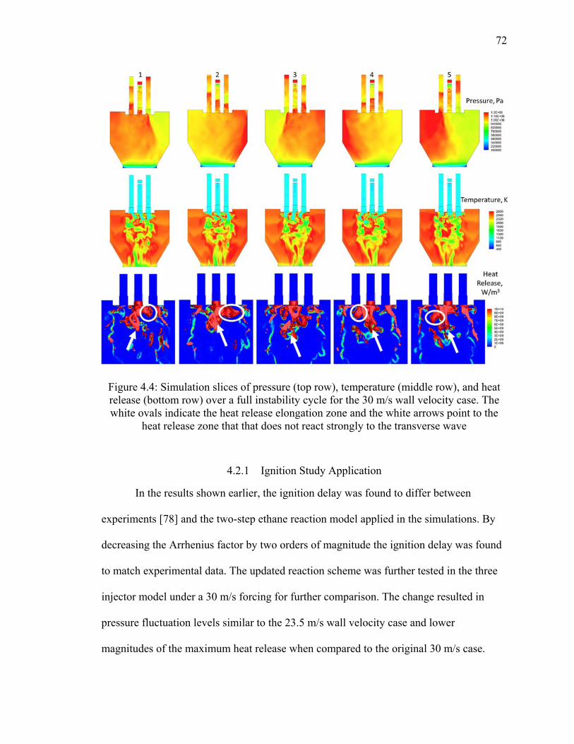
72

Figure 4.4: Simulation slices of pressure (top row), temperature (middle row), and heat release (bottom row) over a full instability cycle for the 30 m/s wall velocity case. The white ovals indicate the heat release elongation zone and the white arrows point to the

heat release zone that that does not react strongly to the transverse wave

4.2.1 Ignition Study Application

In the results shown earlier, the ignition delay was found to differ between

experiments [78] and the two-step ethane reaction model applied in the simulations. By

decreasing the Arrhenius factor by two orders of magnitude the ignition delay was found

to match experimental data. The updated reaction scheme was further tested in the three

injector model under a 30 m/s forcing for further comparison. The change resulted in

pressure fluctuation levels similar to the 23.5 m/s wall velocity case and lower

magnitudes of the maximum heat release when compared to the original 30 m/s case.

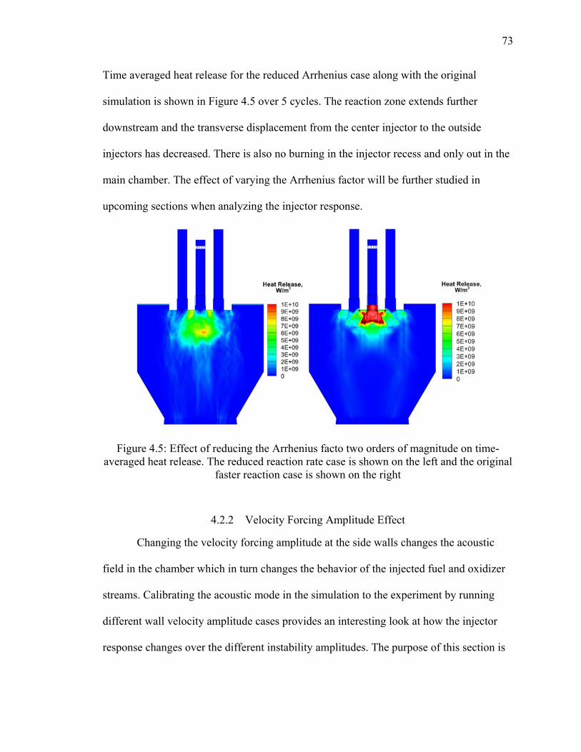
73

Time averaged heat release for the reduced Arrhenius case along with the original

simulation is shown in Figure 4.5 over 5 cycles. The reaction zone extends further

downstream and the transverse displacement from the center injector to the outside

injectors has decreased. There is also no burning in the injector recess and only out in the

main chamber. The effect of varying the Arrhenius factor will be further studied in

upcoming sections when analyzing the injector response.

Figure 4.5: Effect of reducing the Arrhenius facto two orders of magnitude on time-averaged heat release. The reduced reaction rate case is shown on the left and the original

faster reaction case is shown on the right

4.2.2 Velocity Forcing Amplitude Effect

Changing the velocity forcing amplitude at the side walls changes the acoustic

field in the chamber which in turn changes the behavior of the injected fuel and oxidizer

streams. Calibrating the acoustic mode in the simulation to the experiment by running

different wall velocity amplitude cases provides an interesting look at how the injector

response changes over the different instability amplitudes. The purpose of this section is

74

to show what the effect the different instability amplitudes have on the injection response

and chamber flowfield. Results are presented for the three instability amplitudes

summarized in Table 4.1.

Table 4.1: Instability amplitudes for 5, 23.5 and 35 m/s forcing

Case Name Forcing Amplitude, m/s

Forcing Frequency, Hz

P’, kPa P’/Pc, %

Low 5 2035 83 8% Medium 23.5 2035 510 46%

High 35 2035 790 68%

The strength of the transverse wave grows almost linearly as the amplitude

increases. Figure 4.6 shows a one-dimensional representation of the transverse velocity

mode shape in the chamber filtered at the first acoustic frequency. The peak amplitude is

about five times the forcing amplitude in each case. The stronger waves further increase

the amplitude of heat release fluctuations and displacement from the center injector

outwards towards the side injectors as shown in Figure 4.7.

Figure 4.6: Transverse velocity mode shape across the chamber width for varying forcing conditions.

75

Figure 4.7: Heat release fluctuation mode shape across the chamber width for varying forcing conditions.

Increasing the forcing amplitude results in enhanced mixing in the combustion

chamber. This can be seen in the time-averaged flowfields for the different cases. Figure

4.8 shows the time-averaged temperature flowfield for the three different forcing

amplitudes. The low amplitude forcing allows the oxidizer jets to persist largely

undisturbed further into the combustion chamber than the other two cases. Increasing the

amplitude decreases the penetration length of the jets, In the highest amplitude case the

temperature shows that combustion takes place near the injection plane because the

stronger transverse waves enhance mixing of the fuel and oxidizer. There are also hot

combustion products from the side interacting in the region.

Figure 4.8: Effect of varying wall velocity amplitudes on the temperature flowfield using time-averaged results over 5 instability cycles.

76

The varying levels of instability result in different amounts of mixing for each

case. The resulting spatial distributions of fuel and oxidizer mass fractions can be seen in

Figure 4.9 and Figure 4.10. The low transverse wave amplitude that results from 5 m/s of

forcing allows the fuel to spread out around the injector near the injection plane and to

move into the chamber. As the amplitude increase there is less spreading of the fuel, both

in the transverse direction and the axial direction. In the medium amplitude case there is

still measurable axial penetration but the high concentration (85%) region that

surrounded the injector is gone. The highest amplitude further retards the penetration

depth.

The oxidizer on the other hand shows more spreading at higher amplitudes. This

is because the chamber is an oxidizer rich environment and not all of the oxidizer will be

consumed. For the low amplitudes, the 10% oxygen isosurface shows that the oxidizer

jets are largely undisturbed as it moves through the chamber. Combustion is also taking

place further from the injection plane as evident by the larger amounts of oxidizer present

downstream of the center injector. Contrast this with the medium and high cases which

show regions of higher oxidizer concentration near the injection plane. The high

amplitude case also shows that there is significant interaction of the side oxidizer jets and

the bypass flow, especially near the top of the chamber where the 10% oxygen isosurface

shows large disturbances compared with the 5/ms case.

77

Figure 4.9: Effect of varying wall velocity amplitudes on local ethane fuel mass fraction using time-averaged results over 5 instability cycles. Ethane isosurfaces are shown at

85%, 25% and 10%.

Figure 4.10: Effect of varying wall velocity amplitudes on oxidizer mass fraction using time-averaged results over 5 instability cycles. Oxygen isosurfaces are shown at 10%,

20% and 30%

The effect of higher amplitude forcing on the combustion heat release is an

increase in transverse heat release displacement from the center injector towards the

oxidizer injectors and a decrease in the longitudinal heat release extension into the

chamber as fuel and oxidizer are mixed and burned closer to the injector face. Time

averaged heat release is presented in Figure 4.11 as an isosurface and a contour slice

through the center of the chamber. Higher heat release can be seen in the side injectors

78

with the 5 m/s forcing condition. This may be due to more fuel making its way to the side

injectors that is burned off more quickly in the higher forcing case. Moving to higher

forcing conditions, the region around all three of the injectors shows more activity as the

fuel begins mixing more with oxygen from all three injectors.

Figure 4.11: Time averaged plots of heat release for different wall velocity conditions with an isosurface at 1.0E+10 W/m3.

4.3 Comparison with Experiments

Results from different forcing cases are compared to the experiments in this section

with a focus on the 30 m/s case. The goal of the three injector model is to match the

injector response and the limit cycle of the configuration that corresponds to the highest

amplitude instability observed experiment. Calibrating the acoustic field in the simulation

to this level revealed that the best match is obtained for a wall forcing between 30 m/s

and 35 m/s. Results are presented to show how the acoustic field matches experimental

configurations 1, 2 and 3 and how the center injector responds to transverse oscillations.

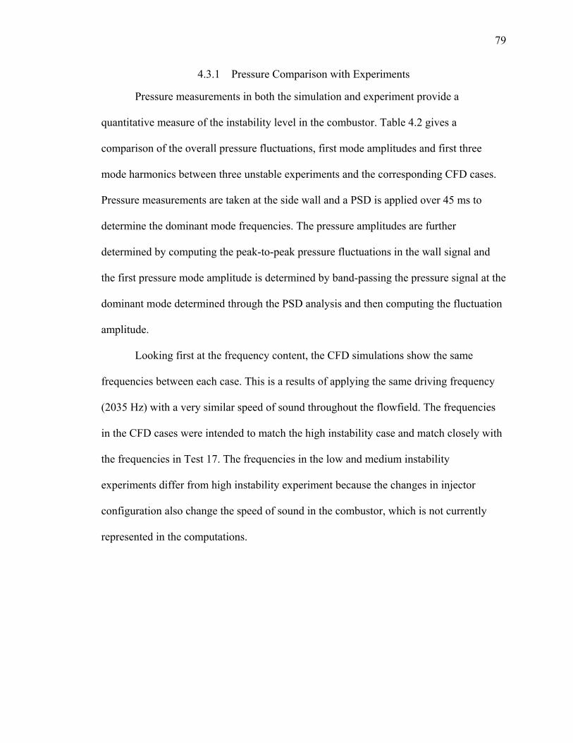
79

4.3.1 Pressure Comparison with Experiments

Pressure measurements in both the simulation and experiment provide a

quantitative measure of the instability level in the combustor. Table 4.2 gives a

comparison of the overall pressure fluctuations, first mode amplitudes and first three

mode harmonics between three unstable experiments and the corresponding CFD cases.

Pressure measurements are taken at the side wall and a PSD is applied over 45 ms to

determine the dominant mode frequencies. The pressure amplitudes are further

determined by computing the peak-to-peak pressure fluctuations in the wall signal and

the first pressure mode amplitude is determined by band-passing the pressure signal at the

dominant mode determined through the PSD analysis and then computing the fluctuation

amplitude.

Looking first at the frequency content, the CFD simulations show the same

frequencies between each case. This is a results of applying the same driving frequency

(2035 Hz) with a very similar speed of sound throughout the flowfield. The frequencies

in the CFD cases were intended to match the high instability case and match closely with

the frequencies in Test 17. The frequencies in the low and medium instability

experiments differ from high instability experiment because the changes in injector

configuration also change the speed of sound in the combustor, which is not currently

represented in the computations.

80

Table 4.2: Pressure fluctuation amplitude and frequency comparison between the three injector simulations and experiments from a pressure measurement at the side wall

CFD Wall velocity

(m/s)

Driving frequency,

(Hz) P’/Pc, % P1’/Pc, % 1W (Hz) 2W (Hz) 3W (Hz) 5 2035 8 7 2039 4065 6104 23.5 2035 47 30 2039 4065 6104 30 2035 56 38 2039 4065 6104 Experiment Configuration P’/Pc, % P1’/Pc, % 1W (Hz) 2W (Hz) 3W (Hz) Test 23 low 17 5 1880 3516 5249 Test 18 medium 42 26 1807 3625 5444 Test 17 high 64 50 2026 4065 6091

Comparing the pressure fluctuation amplitudes, the 5 m/s case most closely

matches the low instability experiment configuration. The first mode pressure

fluctuations differ by only 2% of the mean chamber pressure. The remaining modes in

the experiment however are much stronger which is why the total pressure fluctuations

are 9% higher. The 23.5 m/s matches well with Test 18, different by only 5% of the total

pressure fluctuations and 4% of the first mode fluctuations. The 30 m/s case matches

most closely with the high instability experiment although the pressure fluctuations are

lower. The overall fluctuations differ by 8% of the mean chamber pressure and 11% of

the first mode pressure fluctuations.

A comparison of PSD plots is presented between the CFD cases and experiments

in Figure 4.12. The first three frequencies in each case are the same as those presented in

Table 4.2. The simulations generally show more prominent higher order harmonics

whereas the experiment signal decays more rapidly. This is in part due to the increased

noise in the experiment signal, which is almost an order of magnitude higher. The 30 m/s

case compares well with Test 17 up to 20 kHz. The 23.5 m/s also shows a prominent

81

signal up to 20 kHz whereas in the experiment the prominent peaks are only visible up to

the 4th harmonic. The 5 m/s frequencies actually decay more rapidly than the experiment

and a stronger mode is seen at the fourth frequency that is not visible in the simulation.

This shows that the higher modes and harmonics play a larger role in the experiment than

is being modeled in the 5 m/s simulation. Given that only single frequency forcing

function has been applied, the frequencies seem to match quite well.

Figure 4.12: PSD analysis of the left wall pressure signal for varying velocity amplitude boundary conditions and experiment configurations low, medium and high.

A comparison of mode pressure amplitudes is presented in Figure 4.13 between

the same simulations and experimental tests. Pressure is first measured at the side wall

where a pressure antinode lies and is then band-passed around the first four acoustic

frequencies determined through the PSD analysis.

82

A similarity that can be seen between the simulation and experiment is that the

first mode grows the largest over the different instability levels. The first mode grows

from around 7% to around 40% of the mean chamber pressure. A difference between the

experiment and simulation is the limit cycle fluctuation consistency. The mode

fluctuation amplitudes may vary in the experiment up to 5% while in the CFD simulation

the limit cycle remains almost constant. A few small fluctuations can be seen in the 23.5

m/s case. Comparing the low instability test with the 5 m/s case, the mode pressure

amplitudes sometime differ by 100%. The experiment shows stronger higher order mode

fluctuations that are not present in the simulation. In all the experimental tests, the higher

mode amplitudes exceed those in the simulations. Obtaining higher mode accuracy would

probably require forcing at multiple frequencies. For the higher instability case,

implementing a single frequency forcing function appears to provide a good first order

approximation of the pressure field.

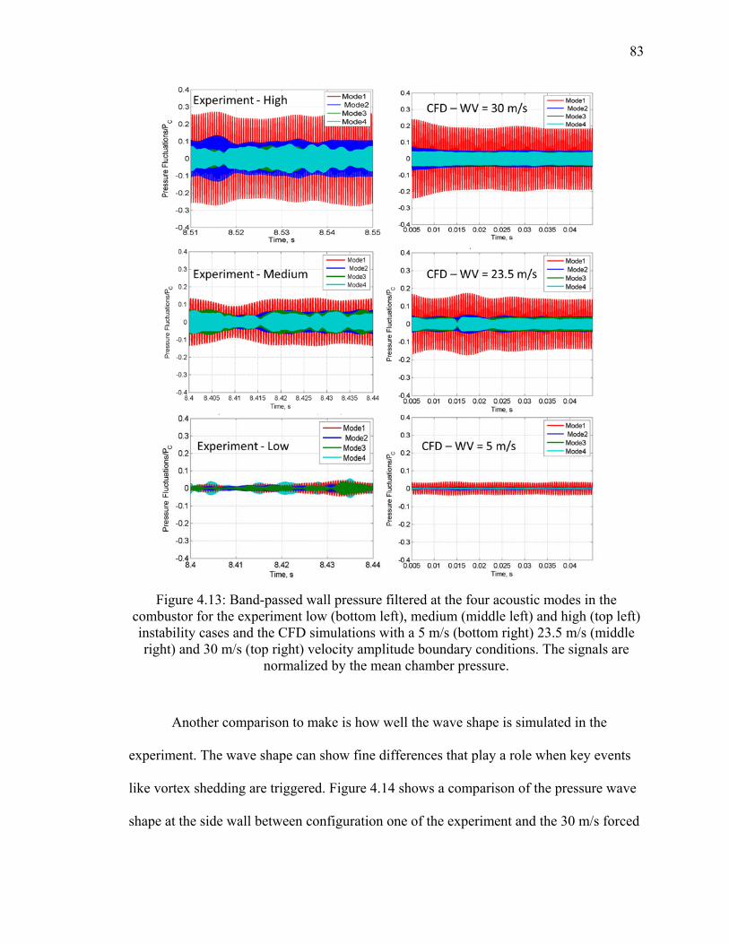
83

Figure 4.13: Band-passed wall pressure filtered at the four acoustic modes in the combustor for the experiment low (bottom left), medium (middle left) and high (top left) instability cases and the CFD simulations with a 5 m/s (bottom right) 23.5 m/s (middle right) and 30 m/s (top right) velocity amplitude boundary conditions. The signals are

normalized by the mean chamber pressure.

Another comparison to make is how well the wave shape is simulated in the

experiment. The wave shape can show fine differences that play a role when key events

like vortex shedding are triggered. Figure 4.14 shows a comparison of the pressure wave

shape at the side wall between configuration one of the experiment and the 30 m/s forced

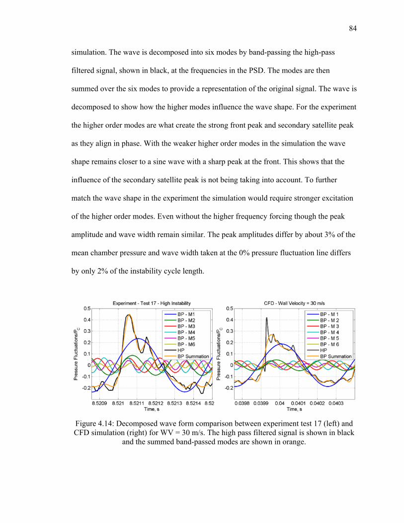
84

simulation. The wave is decomposed into six modes by band-passing the high-pass

filtered signal, shown in black, at the frequencies in the PSD. The modes are then

summed over the six modes to provide a representation of the original signal. The wave is

decomposed to show how the higher modes influence the wave shape. For the experiment

the higher order modes are what create the strong front peak and secondary satellite peak

as they align in phase. With the weaker higher order modes in the simulation the wave

shape remains closer to a sine wave with a sharp peak at the front. This shows that the

influence of the secondary satellite peak is not being taking into account. To further

match the wave shape in the experiment the simulation would require stronger excitation

of the higher order modes. Even without the higher frequency forcing though the peak

amplitude and wave width remain similar. The peak amplitudes differ by about 3% of the

mean chamber pressure and wave width taken at the 0% pressure fluctuation line differs

by only 2% of the instability cycle length.

Figure 4.14: Decomposed wave form comparison between experiment test 17 (left) and CFD simulation (right) for WV = 30 m/s. The high pass filtered signal is shown in black

and the summed band-passed modes are shown in orange.

85

4.3.2 Injector Combustion Response Comparison

Applying the oscillating velocity boundary condition has been shown to

successfully mimic the acoustic fluctuation levels in the experiments. To further

investigate how the center injector responds to transverse oscillations dynamic mode

decomposition (DMD) is applied to the simulation heat release and a comparison is made

with the experimental CH* measurements which is a qualitative representation of the heat

release. DMD is performed on the same window volume in the simulation as captured by

the experimental line-of-sight measurement. The window volume is first integrated

through to create a 2D image in the simulation for a more direct comparison to the

experiment.

DMD is used to compare three cases: the original 30 m/s case, the reduced

reaction rate case, and the experiment. The DMD results show that the reduced reaction

rate case is a better match to the experiment in terms of the combustion response, despite

the lower overall amplitude. DMD of the window area at the first acoustic mode is

presented in Figure 4.15 over half of an instability cycle. The one-dimensional pressure

and transverse velocity profile across the chamber width are shown on the left for

reference. The wave starts at the window center and moves left at the first time point. It

then reaches the left wall in row 3, is reflected back and ends up in the window center

again, moving right in row 6.

Before delving into the detail about what might be happening in the window, a

simple comparison between columns b, c and d shows that the heat release contours in

the third and fourth columns have the closest matching spatial and temporal responses.

86

This indicates that the reaction model plays a vital role in simulating the combustion

response of the center injector.

As a reminder the DMD heat release response at the primary acoustic frequency

shows the response of the injector to the transverse velocity field and is not pressure

coupled. This is because there is a pressure node and velocity anti-node at the injector

location. In other words, when the wave is at the center of the chamber, the injector is

subjected to the strongest transverse velocity amplitude. The strongest heat release

response for the fast reaction simulation is observed in snapshot 2B when the wave has

just passed the chamber center. The slower reaction rate and experiment on the other

hand show that the strongest reaction occurs after the wave has passed the center (5c and

4d) and is returning to the chamber center. Each of the three cases are similar in that as

the transverse wave nears a side wall, the flow recovers from the velocity impulse and the

reacting zone is convected further downstream in the widow. The difference occurs in

how the heat release spreads when subjected to the transverse wave. Figure 4b shows a

small patch of heat release extending into the right window region from the top window

boundary as the transverse wave moves to the right but has not yet reached the window.

This implies the reaction starts without aid from the transverse wave. On the other hand

the reaction zone in the experiment and slowed reaction case starts shifting to the right

(5c and 5d) at the moment the transverse wave has reached the left window boundary and

is moving towards the right.

The DMD of the second acoustic mode is shown in Figure 4.16. One may infer

that the resulting combustion response is an effect of pressure coupling as the center

injector lies at the second acoustic pressure antinode. As in the case of the first mode

87

results, the slow reaction simulation and experiment show similar spatial and temporal

heat release and CH* responses. When the transverse wave is at the center of the window

(row 1 and 6) a difference is observed between the fast reaction and the slow reaction

simulation and experiment. Whereas the latter show very little response, the fast reaction

case shows a strong central reacting region that expands outwards away from the window

center looking from 1b to 2b. The region expands until the transverse wave reaches the

left wall, at which time the reaction appears to be partially extinguished (4b). The slowed

reaction simulation and experiment are similar until about the fourth row when the

experiment (4d) shows a much strong energy pulse. The reaction seems to dissipate

thereafter as the wave returns (5c, 5d) and the two heat lobes form again as the wave is at

the chamber center. Overall between the first and second modes, the slowed reaction

simulation shows some striking resemblance to the experiment.

88

Figure 4.15: Dynamic mode decomposition at the first acoustic mode of heat release in the simulation and CH* in the experiment. Simulation results are presented for the 30 m/s

wall velocity case with a faster reaction and slower reaction achieved by adjusting the Arrhenius factor. The corresponding pressure and transverse velocity profile in the

chamber for each time point is shown for reference. The white arrows show the direction the heat release is moving to.

89

Figure 4.16: Dynamic mode decomposition at the second acoustic mode of heat release in the simulation and CH* in the experiment. Simulation results are presented for the 30 m/s

wall velocity case with a faster reaction and slower reaction achieved by adjusting the Arrhenius factor. The corresponding pressure and transverse velocity profile in the

chamber for each time point is shown for reference.

90

4.3.3 Reaction Investigation

Having shown the similarities between the slowed reaction simulation and the

experiment, an investigation is made into the differences between the faster and slower

reaction simulations. Results are used to develop an understanding of why the difference

exists in the simulations and to help understand how the combustion from the center

injector is affected by the transverse wave.

The DMD of the first acoustic mode is shown in Figure 4.17 for the faster and

slower reaction simulations. Contours of the fuel and oxidizer are overlaid in the first and

second columns respectively. In the first row the transverse wave is at the center of the

window and is moving from right to left, subjecting the reacting zone to a strong

transverse velocity. Both cases show the fuel and oxidizer moving left. In the case of the

faster reaction, the fuel is quickly consumed in the upstream section of the window,

giving rise to a peak heat release (a1). For the slow reaction only a small amount of

burning takes place in the upper left corner of the window (c1). There is also less oxygen

in the bottom left of the window than seen in the fast reaction case as the large reacting

zone on the right absorbs the oxygen (d1) that would have moved left under the

transverse wave. The transverse wave also appears to have blocked off fuel from entering

the top right of the window (c1) for both cases.

As the transverse wave continues to move left and leaves the window, the faster

reaction case shows the ethane jet burning through the left-side as the right of the window

fills up with oxygen (a1 and b1). The reacting zone continues to convect further

downstream, consuming fuel and oxidizer and clearing the window (b5). In the slower

reaction case as the transverse wave passes by the window the large reaction zone

91

dissipates and the remaining oxidizer convects diagonally downward (d2). As more fuel

and oxidizer mix the left reaction zone finally begins to grow and moves downstream

with the oxidizer starting to fill the right window volume (c4 and d4), but not as much as

in the faster reaction case because there is less fill time in this case (due to the slower

reaction).

In row four, the transverse wave has reflected off the left wall and is beginning to

move back to the window. An ethane jet has started to reappear in both cases in the right

side window, more clearly visible in the slower reaction case (c4). The fuel is injected in

a concentrated amount and burns immediately in the faster reaction case with the oxygen

that has filled the right side of the window. In the slower reaction case, burning does not

appear until row 5 and only a small amount is visible in the top right window corner (d5).

The left reaction zone finally reaches a maximum heat release (c5) in contrast to the fast

reaction case which reaches a maximum heat release in row 2. In the last row the

transverse wave has again made it to the window center and the same cyclic process

begins once again.

The behavior shows that the reaction time influences the spatial location of heat

release as fuel and oxidizer are displaced due to the transverse wave which also cuts off

the fuel supply. The reaction time then further influences the spatial location of fuel and

oxidizer as they are either consumed earlier or later in the process.

92

Figure 4.17: Dynamic mode decomposition at the first acoustic mode for the 30 m/s wall velocity cases with a faster reaction and slower reaction achieved by adjusting the

Arrhenius factor. Fuel (orange) and oxidizer (white) mass fraction are overlaid for each case to illustrate the relationship with the reacting zones. The time point for each row is

the same as the rows presented in Figure 4.15 and Figure 4.16.

93

Moving on to the second acoustic mode the pressure effect of the transverse wave

can be analyzed. The same layout is presented as before. The fuel and oxidizer appear in

different spatial location as the first DMD mode because they have also been

decomposed through the DMD process. The spatial heat release locations between both

cases start off very different although the oxidizer and fuel locations are similar (row 1).

Ethane is seen upstream in the center of the window with a core flow of oxidizer mixed

in the same central location (c1 and d1) that then spreads out further downstream. The

faster reaction case shows immediate burning between the fuel and oxidizer; however,

the slower reaction case shows only two side heat release lobes even though fuel and

oxidizer are mixing in the central region.

With the transverse wave at the center, the window region is at a higher pressure

in the second acoustic mode pressure cycle. The higher pressure appears to condense the

fuel into a bubble (a2 and c2) in the center of the oxidizer core which convects

downstream as the wave passes and pressure begins decreasing. In the faster reaction

case, this burns a tunnel through the oxidizer core (b3) and the heat release increases as

the fuel bubble is consumed. This is the point when the most heat release is seen and is

also when the pressure is at a minimum in the chamber. In the slower reaction case, the

bubble and oxidizer are more diffuse and more heat release is spread out but starts to

become concentrated (c3). Part of the diffusivity may be an effect of the difference

between the pressure fluctuation amplitudes.

The central oxygen is completely consumed in the fast reaction case by point 4

(b4) and the heat release becomes partially extinguished. For the slow reaction this occurs

in row five (d5). Also at point 5, fuel and ox begin to enter the window from the top

94

central region (row 5) as the transverse wave returns. Oxygen fills the central core region

more in the faster reaction simulation as there is more fill time from when the core

reaction ends. The wave then returns to the center of the chamber and the two side heat

release lobes reappear in the slower reaction simulation (d6) as ethane fuel reacts with an

outer oxidizer rich region possibly due to the adjacent oxidizer injectors. In the faster

reaction simulation, the ethane fuel appears to wrap around the central oxidizer core (a6).

With the wave at the window center, the fuel will condense due to the increased pressure

and the process will start once again.

The reaction time also plays an important role in the spatial location of the fuel,

oxidizer and heat release. Some of the difference may be due to the different pressure

fluctuation amplitudes between the simulations but the larger difference in heat release

spatial location appears to be due to the reaction time.

Overall, comparing both simulations, the effect of the reaction time on the

combustion process is illustrated with coupling to the transverse mode. The results show

how the spatial locations of fuel, oxidizer and heat release change over time. And the heat

release locations most closely match the decomposed CH* measurements in the slower

reaction case, providing an interesting insight into what may be happening in the

experiment.

95

Figure 4.18: Dynamic mode decomposition at the first acoustic mode for the 30 m/s wall velocity cases with a faster reaction and slower reaction achieved by adjusting the

Arrhenius factor. Fuel (orange) and oxidizer (white) mass fraction are overlaid for each case to illustrate the relationship with the reacting zones. The time point for each row is

the same as the rows presented in Figure 4.15 and Figure 4.16.

96

4.4 Conclusion

The objective of this study was to investigate the application of the three injector

model as a test bed for evaluating the combustion response of the center injector to

transverse instability oscillations. The method applied a wall velocity forcing function at

the side walls calibrated to the experimental instability levels. A cycle analysis showed

that the transverse wave produced is angled due to reflection across the converging

chamber section. The effect of the wave on the injector heat release response was found

to be three dimensional in nature. Zones near the front and back walls remained

stationary while large fluctuations were observed in the central region where the injector

is located.

A further analysis on the effect of different forcing amplitudes showed that stronger

forcing resulted in increased mixing and stronger heat release fluctuations near the center

injector. The heat release zones also spread further outward towards the side walls as fuel

was burned in the side oxidizer jets.

Comparison with the experiment showed that applying a single frequency velocity

oscillation was a successful method to match the experiment high instability pressure

fluctuations in both amplitude and frequency. Multi-frequency forcing was also proposed

as a needed step to increase the accuracy in matching pressure.

The heat release response of the injector was further compared with CH*

measurements in the experiment by apply DMD analysis. The results showed that the

simulation was able to match the spatial and temporal behavior for the first two DMD

modes. Furthermore it was found the reaction rate played an important role in the

combustion response with the slower of the two reaction rates matching more closely

97

with the experiment. The comparison is still a qualitative assessment but the results show

promise for being able to match unstable heat release between simulations and

experiments.

A further investigation was performed to explore the effect of the transverse wave

and the reaction rate on the fuel and oxidizer field and their relation to local heat release.

DMD was again applied and the analysis was performed on the strongest two acoustic

modes. The first mode was interpreted as having a velocity effect on the field while the

second mode provided local pressure fluctuations. The change in local heat release was

shown to be an effect of how the fuel and oxidizer mixed under local pressure and

velocity fluctuations and the reaction rate of the simulation. This further demonstrates the

importance of determining the correct reaction rate since it can completely change the

location of oxidizer, fuel and local heat release.

98

CHAPTER 5. COMPUTATIONAL STUDY OF TRANSVERSE INSTABILITY MECHANISMS

The response of a shear coaxial injector was previously studied in a longitudinal

configuration under self-excited combustion instability [11]. Here the seven injector

simulation is applied to investigate the response of similar injectors to transverse

instability, which is also self-excited and the same single-step methane reaction model is

applied [11]. A focus of the chapter is on exploring the relationship of the injectors to the

physical mechanisms driving instability in the combustor as postulated in a prior study

[29]. The outside injectors appear to play an influential role in the vortex shedding

process which can directly impact instability amplitudes.

The chapter is organized as follows. First an overview is given of the behavior of

the seven injector simulation instability. Subsequent sections are then organized

sequentially based upon instability amplitudes. The first section covers the initial

transient startup of the simulation. Next, the transition to a low instability is investigated

to learn what influence the driving injectors may have on the instability. The following

section focuses on the growth to a higher mode of instability and what may influence the

behavior switch. The last section covers growth to the most extreme level of instability

reached in the simulation and subsequent damping of the system. The results presented

here provide the initial step to further understanding the TIC behavior and introduce a

few driving processes that can be the focus of future studies.

99

5.1 Overview of Instability Behavior

The seven injector simulation produces a range of instability amplitudes as shown

in Figure 5.1. After recovery from ignition, low amplitude pressure fluctuations develop

in the combustor ranging from 10-20 % of mean chamber pressure with the primary

acoustic frequency centered at 2014 Hz. The mean chamber pressure during this time lies

between 0.9 and 1.0 MPa and later reaches a peak of 1.05 MPa. At 7.4 ms the combustor

transitions to stronger growth and a maximum pressure fluctuation amplitude, 70% of

mean chamber pressure, is reached. Afterwards pressure fluctuations dampen and a series

of increasing and decreasing fluctuations arise until the simulation ends. Performing a

spectrogram analysis on the signal, which applies a short-time Fourier transform, shows

higher transverse modes arise as the instability amplitude grows. The primary transverse

mode appears during the low amplitude instability period and as higher amplitude

pressure fluctuations are reached harmonics of the primary frequency appear.

Figure 5.1: Overview of instability produced in the seven injector simulaiton showing wall pressure fluctuations (top) and the corresponding freqency content (bottom).

100

As the number of excited modes in the chamber changes so does the amplitude of

each mode. This is shown in Figure 5.2 where the left wall pressure is band-pass filtered

for the first three modes which are plotted along with the high-pass filtered pressure

signal. The simulation starts off with a strong first mode that grows until the peak

amplitude is reached. At this time, around 11 ms the first mode starts to decay.

Interestingly around 15 ms the second mode becomes the dominant mode as the pressure

fluctuation amplitudes reach a low point. And around 20 ms the second mode dampens

and the first mode becomes the dominant mode again. The transition to a second mode

instability is discussed in the last section of this chapter.

The pressure signal shows growth and decay with many different levels of

instability. The advantage of applying CFD is that these phenomena can be more fully

explored.

Figure 5.2: Left wall high-pass filtered pressure and band-pass filtered pressure at the three modes.

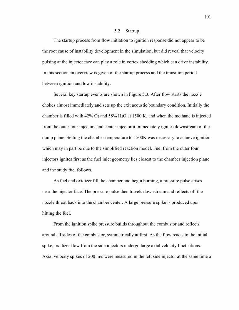
101

5.2 Startup

The startup process from flow initiation to ignition response did not appear to be

the root cause of instability development in the simulation, but did reveal that velocity

pulsing at the injector face can play a role in vortex shedding which can drive instability.

In this section an overview is given of the startup process and the transition period

between ignition and low instability.

Several key startup events are shown in Figure 5.3. After flow starts the nozzle

chokes almost immediately and sets up the exit acoustic boundary condition. Initially the

chamber is filled with 42% O2 and 58% H2O at 1500 K, and when the methane is injected

from the outer four injectors and center injector it immediately ignites downstream of the

dump plane. Setting the chamber temperature to 1500K was necessary to achieve ignition

which may in part be due to the simplified reaction model. Fuel from the outer four

injectors ignites first as the fuel inlet geometry lies closest to the chamber injection plane

and the study fuel follows.

As fuel and oxidizer fill the chamber and begin burning, a pressure pulse arises

near the injector face. The pressure pulse then travels downstream and reflects off the

nozzle throat back into the chamber center. A large pressure spike is produced upon

hitting the fuel.

From the ignition spike pressure builds throughout the combustor and reflects

around all sides of the combustor, symmetrically at first. As the flow reacts to the initial

spike, oxidizer flow from the side injectors undergo large axial velocity fluctuations.

Axial velocity spikes of 200 m/s were measured in the left side injector at the same time a

102

vortex appeared to be shed from the injector lip. This may indicate that velocity pulses in

the injectors may lead to the production of vortices in the chamber.

Figure 5.3: Simulation startup from initial conditions. The combustor chokes almost immediately (shown left), ignites and produces a pressure wave that reflects of the nozzle

and builds into a pressure spike (shown right) upon interaction with fuel entrained vortices downstream of the injector plane.

Between the ignition spike which reaches peak amplitude around 0.8 ms and the

instability onset around 2.4 ms, fuel and oxidizer are primarily filling the chamber

volume. A pressure trace from the left and side walls of the chamber is shown in Figure

5.4 marked with key events up until the first low amplitude instability peak. Initially the

pressure fluctuations in the chamber remain fairly symmetric about the chamber center in

103

response to the initial pressure spike but become asymmetric as the fuel and oxidizer fill

the chamber volume and combust further downstream. Figure 5.5 shows a pressure slice

in the combustor right before the transition event. Isolated zones of higher pressure can

be noticed. These high pressure locations change constantly over time and appear quite

chaotic but disappear as the low instability cycle develops.

Figure 5.4: Left and right wall pressure measurements showing transition from post-ignition to low amplitude combustion instability

Figure 5.5: As fuel and oxidizer fill the chamber pressure fluctuates in the chamber.

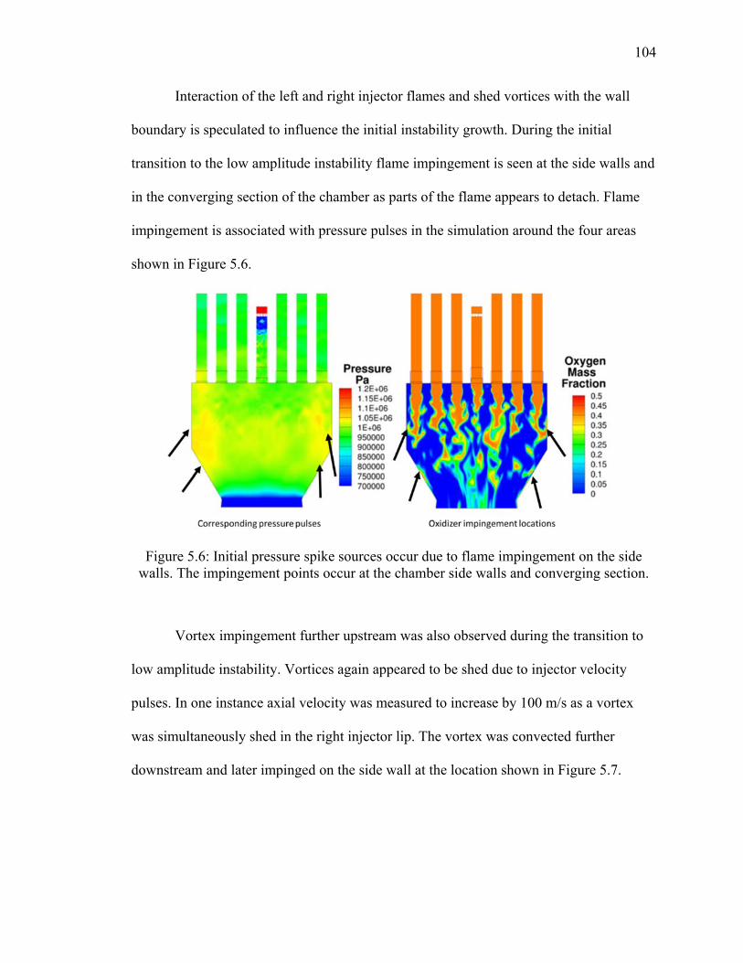
104

Interaction of the left and right injector flames and shed vortices with the wall

boundary is speculated to influence the initial instability growth. During the initial

transition to the low amplitude instability flame impingement is seen at the side walls and

in the converging section of the chamber as parts of the flame appears to detach. Flame

impingement is associated with pressure pulses in the simulation around the four areas

shown in Figure 5.6.

Figure 5.6: Initial pressure spike sources occur due to flame impingement on the side walls. The impingement points occur at the chamber side walls and converging section.

Vortex impingement further upstream was also observed during the transition to

low amplitude instability. Vortices again appeared to be shed due to injector velocity

pulses. In one instance axial velocity was measured to increase by 100 m/s as a vortex

was simultaneously shed in the right injector lip. The vortex was convected further

downstream and later impinged on the side wall at the location shown in Figure 5.7.

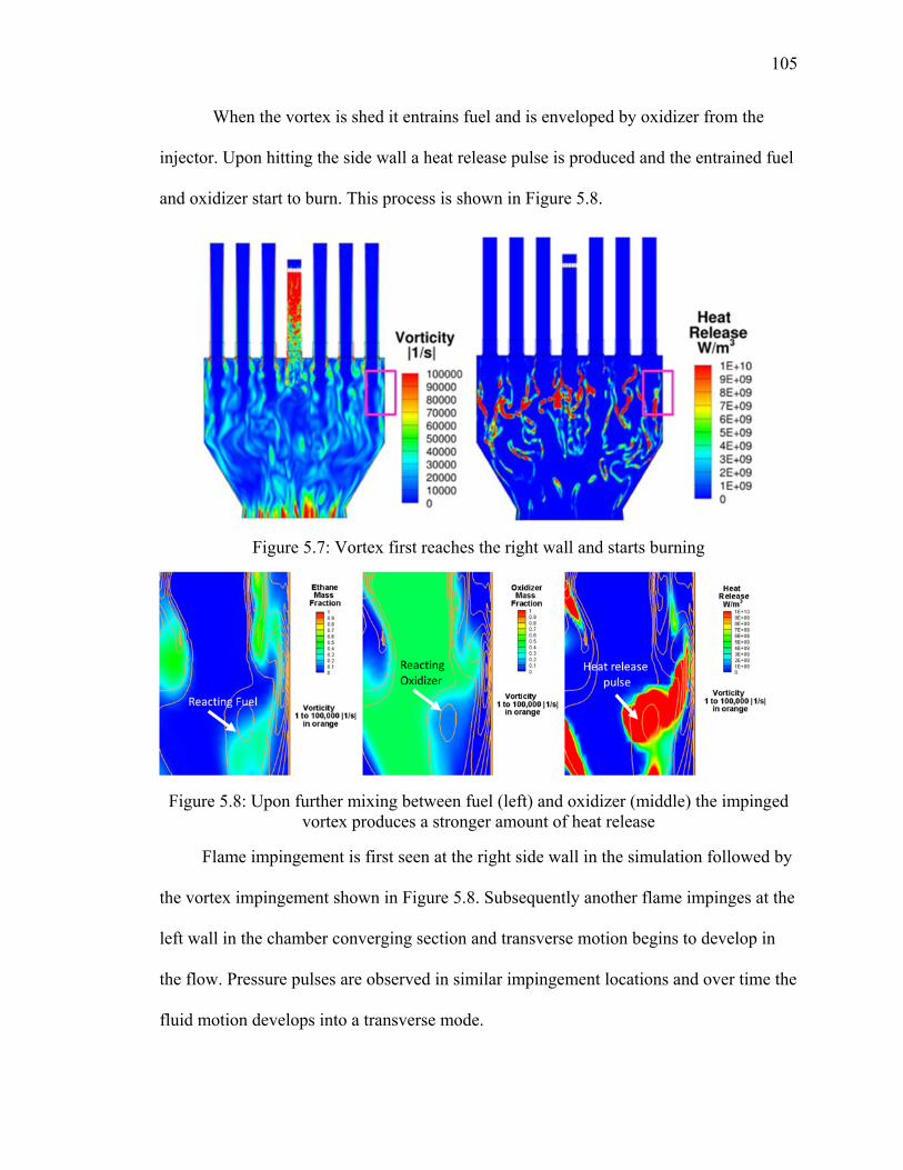
105

When the vortex is shed it entrains fuel and is enveloped by oxidizer from the

injector. Upon hitting the side wall a heat release pulse is produced and the entrained fuel

and oxidizer start to burn. This process is shown in Figure 5.8.

Figure 5.7: Vortex first reaches the right wall and starts burning

Figure 5.8: Upon further mixing between fuel (left) and oxidizer (middle) the impinged vortex produces a stronger amount of heat release

Flame impingement is first seen at the right side wall in the simulation followed by

the vortex impingement shown in Figure 5.8. Subsequently another flame impinges at the

left wall in the chamber converging section and transverse motion begins to develop in

the flow. Pressure pulses are observed in similar impingement locations and over time the

fluid motion develops into a transverse mode.

106

5.3 Low Amplitude Instability

After the initial impulse at 2.5 ms, the instability grows as pictured in Figure 5.9.

This period shows pressure oscillations that grow to amplitudes between 10-20% of the

mean chamber pressure. As the period continues the overall pressure fluctuation

amplitudes remain similar until 7.5 ms.

Figure 5.9: Pressure oscillations at the left and right wall during a lower level of instability.

The low amplitude instability appears to be supported by two similar mechanisms

that started the first transition spike. Pressure, axial velocity and transverse velocity

behavior at the axial center of the left injector is shown during the low instability

amplitude period in Figure 5.10. The corresponding flowfields at a slice through the

center of the chamber are presented in Figure 5.11 and illustrate the process. A vortex is

first shed from the left injector lip (1b) where local pressure is low and tube velocity is

high due to a positive pressure gradient. Next the left injector flame impinges on the side

107

wall (2a) and a pressure pulse appears in the same location that propagates further

upstream. The shed vortex is convected further downstream (3b) and then impinges on

the side wall (4b) but does not appear to cause a heat release pulse as shown (4c). During

this instability amplitude heat release pulses sometimes appear during vortex

impingement and other times are not apparent. From here the cycle repeats with flame

impingement seeming to be the primary source for pressure pulses in the chamber.

Figure 5.10: Pressure, axial velocity and transverse velocity at the left injector during low amplitude instability

108

Figure 5.11: The low amplituide instability driving cycle shows how pressure and heat release pulsations are produced by flame and vorticy impingement with the side wall.

109

5.3.1 Injector Response

Analyzing the injector response helps to point to possible sources of the vortices

in the simulation due to either injector axial velocity pulsations or the resonant motion of

the transverse wave. In most instances the vortices appear to be shed under a large

transverse velocity which suggests the latter.

Measurements at the injection plane for the three driving injectors reveal the

conditions at the injectors throughout the low amplitude instability. The data are band-

pass filtered for axial velocity, pressure and transverse velocity over the first acoustic

frequency for the three left injectors and the first and second acoustic frequency for the

center injector. The results are shown in Figure 5.12. Filtering the data helps simplify the

view of the cycle although removes some detail. The three driving injectors on the left all

respond similarly during the low amplitude instability. The order of events in the cycle

are as follows. First a transverse velocity arises at the left injector face, moving from

right to left. During a transverse motion of the fluid across the injector face a vortex

appears to be shed towards the left wall like shown in Figure 5.11 (1b). Then as the

vortex reaches the wall, pressure rises during impingement of the vortex and

impingement of the injector flame downstream. As the pressure reaches a maximum the

axial velocity retards and then once the pressure pulse fades away axial velocity increases

in the flow.

Characteristic velocities and pressure at the study injector axis are also shown.

The axial velocity and pressure are band-passed at the second acoustic mode and

transverse velocity is band-passed at the first acoustic mode. The band-passed data show

different axial velocity oscillation amplitudes at the 2W frequency which may be due to

110

the complex vorticity field from the study injector choke plate. The transverse velocity

amplitudes at the center injector remain more consistent and are less than the other

injectors, also possibly due to the vorticity field. The pressure and transverse velocity

phase of the center injector leads the other three as the wave moves from side to side.

Figure 5.12: Axial velocity, pressure and transverse velocity band-passed at the main acoustic modes of the four injectors show the influence of the chamber instability at the

transfer point to the injector. The red dashed line indicates the minimum transverse velocity, maximum pressure and maximum axial velocity for injector 1.

As the low amplitude instability period progresses the pressure fluctuation

amplitudes grow. Theoretically the increased heat release in this cycle is causing this. As

the pressure amplitudes grow so do the transverse velocity fluctuations and mixing is

promoted between the fuel and oxidizer. At this time the dominant impingement

mechanism appears to shift from the downstream injector flames to the wall-impinging

111

vortices further upstream. The vorticy sizes also appear to grow and may be producing a

stronger impulse to drive the cycle with.

A time averaged flowfield over the low amplitude instability cycle is shown in

Figure 5.13. The displacement of the injector jets can be seen in the temperature plot and

the vorticity plot shows the variation in vortex impingement location along the side wall.

The location varies anywhere between 4.3 – 9h downstream of the injector face.

Figure 5.13: Averaged flow field plots from 2.5 – 5 ms of temperature (left) vorticity (middle) and heat release (right) show how the instability pushes flow from the side injectors to the middle and vorticity displacement along the wall with heat release.

5.4 High Amplitude Instability

Over the course of the low instability cycle the pressure fluctuation amplitudes

increase slowly and the growth appears to be repeatedly encouraged by flame and vortex

impingement with the side walls. Around 7.4 ms there is a transition to a new level of

instability (indicated in Figure 5.14) that grows rapidly to large oscillations that will

eventually approach 70% of mean chamber pressure.

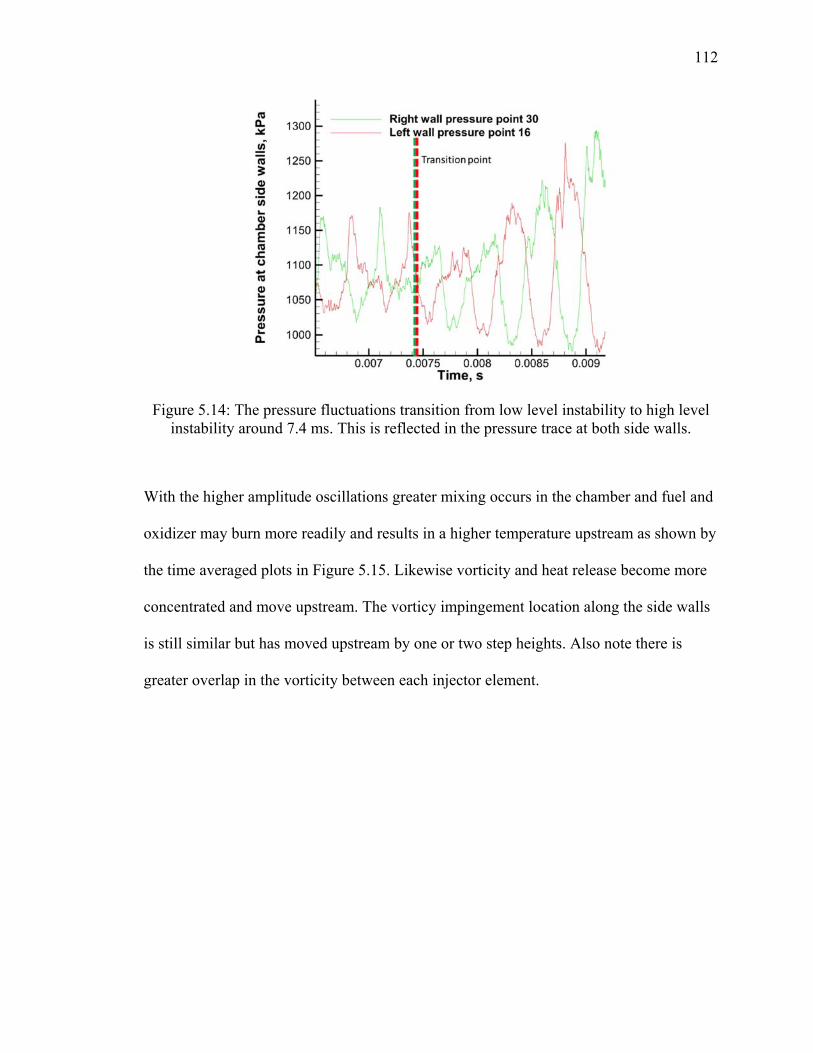
112

Figure 5.14: The pressure fluctuations transition from low level instability to high level instability around 7.4 ms. This is reflected in the pressure trace at both side walls.

With the higher amplitude oscillations greater mixing occurs in the chamber and fuel and

oxidizer may burn more readily and results in a higher temperature upstream as shown by

the time averaged plots in Figure 5.15. Likewise vorticity and heat release become more

concentrated and move upstream. The vorticy impingement location along the side walls

is still similar but has moved upstream by one or two step heights. Also note there is

greater overlap in the vorticity between each injector element.

113

Figure 5.15: Average from 10 -12.5 ms

With increased mixing during the higher amplitude instability the flame no longer

penetrates as far into the chamber. As the pressure fluctuations grow stronger so does the

amplitude of the transverse velocity oscillations while axial velocity fluctuations remain

fairly constant as shown in Figure 5.16. The axial velocity initially reaches a peak

amplitude at the left injector face as the local chamber pressure subsides from the left

side of the chamber. After reflection from the right wall, the transverse wave then returns

to the left injector and causes the initial transverse peak as measured at the injector face.

At this same time a vortex appears to be shed. Following, the vortex impinges at the left

wall at the same time the pressure reaches a peak amplitude. This vortex impingement

cycle remains similar to that during the low amplitude instability period but lacks the

flame impingement further downstream.

114

Figure 5.16: Pressure, axial velocity and transverse velocity fluctuations at the left injector during high instability.

Early on in the high amplitude instability interval, additional vortices start to

impinge between injector elements in addition to the injector impingement at the left wall

at the dominant acoustic frequency. Figure 5.17 provides a look at this process. Fuel

entrained vortices appear to be shed (2a) as the transverse wave passes by each injector

element and convect further downstream. When the transverse wave is reflected to the

left side of the chamber the wave appears to cause three vorticy impingements (1b): one

between the side injector (1) with the wall and the second between vortices shed from left

injector (1) and the adjacent injector (2). It is also possible that a vortex from the third

injector (3) entrains oxidizer and impinges with the right vortex shed from injector 2 to

serve as an additional impulse to further support the instability. At the vortex

impingement locations a corresponding increase is seen in heat release (2c).

115

Figure 5.17: At higher instabilities vortices impinge between injector elements and may further drive the instability to stronger amplitudes.

The interacting vortices appear to drive the instability higher and higher until a

strong instability amplitude is reached around 10.8 ms and pressure concentrations appear

in both the left and right side of the chamber. Just before, the largest transverse velocity

spike at the left injector face appears with an amplitude of 350 m/s. The pressure spike

seen at the left wall is 70% of the mean chamber pressure.

The two strong pressure regions are shown in Figure 5.18 at a later time in the

pressure contour. The second pressure peak appears to have grown out of the nonlinear

shape of the wave as shown in the pressure trace.

116

Figure 5.18: Instability grows to the point that two strong pressure waves appears in the chamber. The dotted black line marks the corresponding point in time of the pressure and

vorticity contours.

The secondary high pressure region acts like a 1W wave and so in some effect may cause

increased vortex shedding as injected fuel is continuously interrupted by the two traveling

waves. The two waves continuously interacting in the flowfield may be reducing the

amount of fuel available for each vortex driven impulse to support the instability cycle.

Pressure fluctuation amplitudes then decrease in the simulation to the levels shown in

Figure 5.19. Interestingly the waves reach a point where they are equally spaced and

alternate from side to side in the chamber as shown at 16 ms forming what appears to be

a 2W mode. Referring back to Figure 5.2, this is the point where the second mode shows

dominance over the first mode. This can now be understood as the simulation has two

strong pressure fronts moving in the chamber acting in a 2W motion.

From here the 2W instability cannot be sustained and a transition to the 1W mode

occurs. The flame flowfield interactions appear to play a very important role in the

instability levels seen in this simulation. The simulation shows that over the different

instability ranges many different processes are produced.

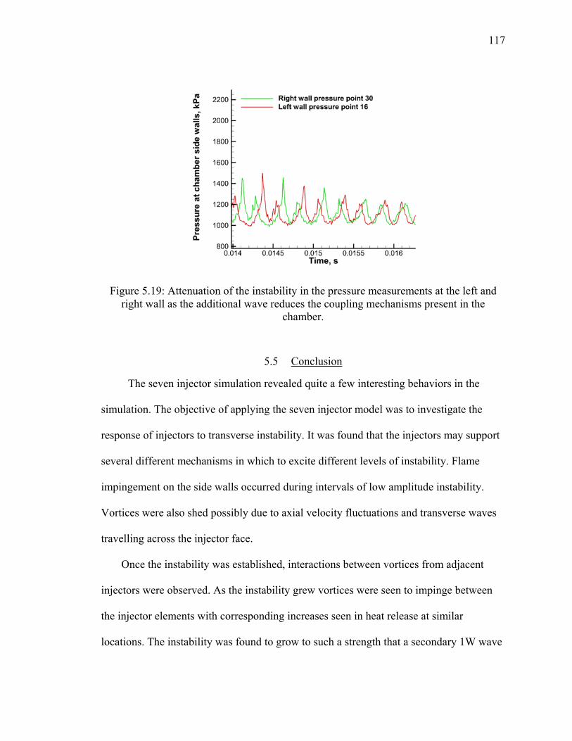
117

Figure 5.19: Attenuation of the instability in the pressure measurements at the left and right wall as the additional wave reduces the coupling mechanisms present in the

chamber.

5.5 Conclusion

The seven injector simulation revealed quite a few interesting behaviors in the

simulation. The objective of applying the seven injector model was to investigate the

response of injectors to transverse instability. It was found that the injectors may support

several different mechanisms in which to excite different levels of instability. Flame

impingement on the side walls occurred during intervals of low amplitude instability.

Vortices were also shed possibly due to axial velocity fluctuations and transverse waves

travelling across the injector face.

Once the instability was established, interactions between vortices from adjacent

injectors were observed. As the instability grew vortices were seen to impinge between

the injector elements with corresponding increases seen in heat release at similar

locations. The instability was found to grow to such a strength that a secondary 1W wave

118

appeared to form from the first and when eventually aligning opposite the first in the

instability cycle appeared to form a 2W mode. The 2W motion was not sustainable in the

chamber, possibly due to the effect on vortex shedding in the chamber. The simulation

reveals some very interesting behavior for future detailed studies.

119

CHAPTER 6. SUMMARY

The objectives of this study were to demonstrate a computational test bed for the

measurements of combustion response and virtual screening of an injector’s susceptibility

to combustion instability using a reduced three-injector model of the TIC configuration,

and to explore a full simulation of a seven-injector combustor for the study of transverse

instability. The last objective was to further develop the integrated subscale modeling and

experimental approach as a key element in a methodology to predict combustion

instability by developing tools that could be used in the analysis of the computational

results and for comparison with experimental measurements.

These objectives were met and the computational models were successfully

applied to investigate the response of shear coaxial injector elements to transverse

instability. The computational test bed consisted of three simulated injector elements with

artificial forcing to generate a transverse instability. The acoustic field generated by

periodically forcing the velocity at the end walls was calibrated to the acoustic field

measured in the experiments. A good match between frequency and amplitude of the first

width (1W) mode was achieved. After demonstrating this matching, the combustion

response of a shear coaxial injector element was compared to high speed imagery of the

flame emission from the experiment.

120

Through application of the seven injector model the response of coaxial injector

elements under transverse instability was further studied, with a focus on the driving

injector elements. Several regimes of instability were observed as the amplitude of the

self-excited instability grew from unorganized low amplitude pressure fluctuations to

very high amplitude resonant oscillations in pressure and velocity. The remaining two

sections of this chapter provide the conclusions of applying these methods along with

recommendations for future activities.

6.1 Conclusions

Applying both models demonstrated that hybrid large eddy simulations can be

used in both a forced and a self-excited manner to predict the combustion response of a

study element to transverse instability. Through the three-injector model it was learned

that applying a single frequency velocity forcing at the end wall can produce high

amplitude instabilities similar to those measured in the experiment. As would be

expected, higher forcing conditions resulted in a stronger response. The higher forcing

conditions showed the reaction zone moved further upstream near the injector face due to

increased mixing between oxidizer and fuel.

Performing a cycle analysis on the three-injector simulation revealed that the

transverse wave is angled due to reflection across the converging chamber section.

Furthermore the effect of the wave on the heat release response was found to be three

dimensional in nature with greater displacement seen near the center where the injector

lies while zones near the front and back wall remained more stationary.

121

The reaction rate in the simulation was also found to have a significant effect on

the spatial and temporal behavior of unsteady heat release and local oxidizer and fuel

concentration. Calibrating the reaction model to ignition delay from shock tube

experiments was found to produce a model that best reflected the response measured in

the second generation experiment.

Dynamic mode decomposition proved to be a powerful tool in analyzing the

flowfield for comparison between the simulations and experiments. The first two modes

from the simulation and experiment both showed that heat release and CH* formation

were interrupted as the wave passed. A limitation of the three injector model as a tool to

study combustion response in subscale experiments is that the calibration process

requires a series of trials to determine the appropriate boundary conditions to match

measured instability amplitudes. The model is sensitive to different boundary conditions

and a single change may require a full new set of calibrating runs.

The seven-injector model showed a remarkably rich set of physics that requires

more study. During the low amplitude instability, the pressure pulsing cycle was

associated with flame impingement at the side walls and vortices shed from the injectors.

The vortex shedding appeared to be related to velocity pulses in the injectors and the

resonant motion of the transverse wave. At higher amplitude instabilities, vortices shed

from the injectors at the dump plane interacted with each other under the influence of

strong transverse velocities. Corresponding increases in heat release were seen near those

locations, possibly driving the instability to higher amplitudes. As the amplitude

approached the highest levels seen in the simulation, a secondary 1W pressure wave

appeared to form from the first. The two 1W wave motions became offset and appeared

122

to develop into a 2W wave motion. The 2W mode was not sustained and eventually

transitioned back into a strong 1W instability.

Although the seven injector simulation provided tremendous detail on how the

self-excitation may occur, one limitation is that self-excitation does not allow for much

control in studying varying levels of injector response.

6.2 Recommendations

The models developed here show significant promise for use in predictive

simulations. There are a few key areas that need improvement which are recommended

here for future work.

One key improvement would be a more quantitative method of comparison

between simulations and experiments. Current methods for heat release comparison are

almost completely qualitative. An approach can be taken on both ends by either finding a

way to determine a more quantitative value of heat release from experiments, or to

calculate CH* from the computational results. In the simulations it would also be helpful

to have a means to better quantify the vortex impingement mechanisms in the

simulations. At this point in the seven injector simulation the investigation was primarily

visual based with a few point measurements taken. A quantitative means to calculate

vorticity and the associated amount of heat release produced through impingement would

be very useful.

Improvements are also needed in the models themselves. A grid sensitivity

analysis is needed for the three injector model and a useful advancement would be to

section the driving inlets to represent the injectors for different configuration of the

123

second generation experiment. The seven injector mesh should also be further refined and

a grid sensitivity study performed. With the third generation experiment being able to test

variable oxidizer post lengths additional simulations can likewise be run in the full

geometry model to investigate how the possible driving mechanisms change in those

conditions. Another useful study would be to investigate how vortices are shed in the

experiment for comparison with the simulation.

Finally, it is clear that modeling the chemical reactions has a major effect on the

result. More work needs to be done to determine the effects of the reaction chemistry, and

to find the reduced set of reactions that can still provide a good match to experiments.

124

REFERENCES

124

REFERENCES

1. Harrje, D. T., and Reardon, F.H. (eds.), “Liquid Propellant Rocket Combustion Instability,” NASA SP-194, 1972.

2. Yang, V., and Anderson, W. (eds.), Liquid Rocket Engine Combustion Instability, Vol. 169, Progress in Astronautics and Aeronautics, AIAA, Washington, D.C., 1995.

3. Sutton, G. P., Rocket Propulsion Elements, Eighth edition, 2010.

4. Oefelein, J. C., Yang, V., “Comprehensive Review of Liquid-Propellant Combustion Instabilities in F-1 Engines,” Journal of Propulsion and Power, Vol. 9, No. 5, Sept. – Oct. 1993, pp. 657 – 677.

5. Menon, S, Jou, W. H., “Large-Eddy Simulations of Combustion Instability in an Axysymmetric Ramjet Combustor,” 28th ASM, AIAA-90-0267.

6. Veynante, D., Pointsot, T., “Large eddy simulation of combustion instabilities in turbulent premixed burners,” Center for Turbulence Research, Annual Research Briefs, 1997.

7. Brookes, S. J., Cant, R. S, Dupere, I. D. J., Dowling, A. P., “Combutational Modeling of Self-Excited Combustion Instabilities, ASME, Vol. 123, April 2001.

8. Selle, L., Benoit, L., Poinsot, T., Nicoud, F., Krebs, W., “Joint use of compressible large-eddy simulation and Helmholtz solvers for the analysis of rotating modes in an industrial swirled burner,” Combustion and Flame, Vol 145, 2006, pp. 194 – 205.

9. Smith, R. J., Computational Investigations of High Frequency Acoustics and Instabilities in a Single-Element Rocket Combustor, PhD Dissertation, Purdue University, West Lafayette, IN, August 2010.

10. Xia, G., Harvazinski, M., Anderson, W., Merkle, C. L., “Investigation of Modeling and Physical Parameters on Instability Prediction in a Model Rocket Combustor,” 47th JPC, AIAA 2011-6030.

11. Harvazinski, M. E., Modeling Self-Excited Combustion Instabilities Using A Combination of Two- and Three-Dimensional Simulations, PhD Dissertation, Purdue University, West Lafayette, IN, May 2012.

12. Garby, R., Selle, L., Poinsot, T., “Large-Eddy Simulation of combustion instabilities in a variable-length combustor,” C. R. Mecanique, Vol. 341, 2013, pp. 220-229.

125

13. Krediet, Prediction of Limit Cycle Pressure Oscillations in Gas Turbine Combustion Systems Using the Flame Describing Function, PhD Dissertation, University of Twente, June 2012.

14. Sankar., S. V., Wang, G., Brena de la Rosa, A., Rudoff., R. C., Isakovic, A., Bachalo, W. D., “Characterization of Coaxial Rocket Injector Sprays Under High Pressure Environments,” ASM, AIAA 92-0228.

15. Glogowski, M., Bar-Gill, M., Puissant C., Kaltz, T., Milicic, M., Micci, M., “Shear Coaxial Injector Instability Mechanisms,” 30th JPC, AIAA 94-2774.

16. Anderson, W. E., Miller, K. L., Ryan, H. M., Pal, S., Santoro, R. J., Dressler, J. L., “Effects of Periodic Atomization on Combustion Instability in Liquid-Fueled Propulsion Systems,” Journal of Propulsion and Power, Vol. 14, No. 5, September-October 1998.

17. Duvvur., A., Chiang, C. H., Sirignano, W. A., “Oscillatory Fuel Droplet Vaporization: Driving Mechanism for Combustion Instability,” Journal of Propulsion and Power, Vol. 12, No. 2, March-April 1996.

18. Rhys, N. O., Hawk, C. W., “Tripropellant Combustion,: Chemical Kinetics and Combustion Instability,” 31st JPC, AIAA 95-3151.

19. Canino, J. V., Heister S. D., Sankaran V., Zakharov, S. I., “Unsteady Response of Recessed-Post Coaxial Injectors,” JPC, AUAA 2005-4297.

20. Long, M. R., Bazarov, V. G., Anderson, W. E., “Main Chamber Injectors for Advanced Hydrocarbon Booster Engines,” 39th JPC, AIAA 2003-4599.

21. Bazarov, V.G., Lyul’ka, L.A., “Study of Self-Oscillatory Liquid Film Flow Regime in Coaxial Air Stream,” Aviatsionnaia Tekhnika, vol. 21, no. 3, 1978, p. 19-24.

22. Andreyev, A. V., Chepkin, V., Fanciullo, T. J., “Autovibration of Coax Injector Elements of O2/H2 Staged Combustion Liquid Rocket Engines, AIAA 95-2837.

23. Canino, J. V., Tsohas, J. Sankaran, V., Heister, S. D., “Dynamic Response of Coaxial Rocket Injectors,” 42nd JPC, AIAA 2006-4707.

24. Smith, D. A., Zukoski, E. E., “Combustion Instability Sustained by Unsteady Vortex Combustion,” 21st JPC, AIAA-85-1248.

25. Poinsot, T. J., Trouve, A. C., Veynante, D. P., Candel, S. M., Esposito, E. J., “Vortex-driven acoustically coupled combustion instabilities,” Journal of Fluid Mechanics, 1987, Vol. 177, pp. 265-292.

26. Ducruix, S., Schuller, T., Durox, D., Candel, S., “Combustion Dynamics and Instabilities: Elementary Coupling and Driving Mechanisms,” Journal of Propulsion and Power, Vol. 19, No. 5, September – October 2003.

27. Morgan, C. J., Response of A Gas-Gas Shear Coaxial Injector to Transverse Instability, Master’s Thesis, Purdue University, West Lafayette, IN, December 2012.

126

28. Miller, K. M., Experimental Study of Longitudinal Instabilities in a Single Element Rocket Combustor,” Master’s Thesis, Purdue University, West Lafayette, IN, May 2005.

29. Sisco, J. C., Measurement and Analysis of an Unstable Model Rocket Combustor, PhD Dissertation, Purdue University, West Lafayette, IN, August 2007.

30. Yu, Y. C., Experimental and Analytical Investigations of Longitudinal Combustion Instability in a Continuously Variable Resonance Combustor (CVRC), PhD Dissertation, Purdue University, West Lafayette, IN, May 2009.

31. Pomeroy, B. R., Measurement and Analysis of Combustion Response to Transverse Combustion Instability, PhD Dissertation, Purdue University, West Lafayette, IN, August 2012.

32. Smith, R., Xia, G., Anderson, W., Merkle, C. L., “Extraction of Combustion Instability Mechanisms form Detailed Computational Simulations,” 48th ASM, AIAA 2010-1152.

33. Smith, R., Xia, G., Anderson, W., Merkle, C. L., “Computational Studies of the Effects of Oxidizer Injector Length on Combustion Instability,” Combustion Theory and Modeling, 2011, DOI:10.1080/13647830.2011.631031

34. Harvazinski, M. E., Huang, C., Sankaran, V., Feldman, T., Anderson, W., Merkle, C. L., Talley, D. G., “Combustion Instability Mechanisms in a Pressure-coupled Gas-gas Coaxial Rocket Injector,” 49th JPC, AIAA 2013-3990.

35. Guéezzenec, N., Mennon, S., “Large-Eddy Simulation of Combustion Instabilities in a Variable-length Combustor,” Comptes Rendus Mecanique, Vol. 341, No. 1-2, 2013, pp. 220-229.

36. Feldman, T. W., Harvazinski, M. E., Merkle, C. L., Anderson, W. E., “Comparison Between Simulation and Measurement of Self-Excited Combustion Instability,” 48th JPC, AIAA 2012-4088.

37. Marshall, W. M., Pal, S., Woodward, R. D., Santoro, R. J., “Combustion Instability Studies Using Gaseous Methane and Liquid Oxygen,” 42nd JPC, AIAA 2006-4526.

38. Marshall, W., Pal, S., Woodward, R., Santoro, R. J., Smith, R., Xia, G., Sankaran, V., Merkle, C. L., “Experimental and Computational Investigation of Combustor Acoustics and Instabilities, Part II: Transverse Modes,” 44th ASM, AIAA 2006-538.

39. Marshall, W. M., Pal, S., Woodward, R. D., Santoro, R. J., “Experimental Study of Transverse Combustion Instabilities in a Multi-Element, Rectangular Rocket Chamber,” 43rd JPC, AIAA 2007-5588.

40. Rey, C., Ducruix, S., Richecoeur, F., Scouflaire, P., Vingert, L., Candel, S., “High Frequency Combustion Instabilities Associated with Collective Interactions in Liquid Propulsion,” 40th JPC, AIAA 2004-3518.

127

41. Bailot, F, Blaisot, J.-B., Boisdron, G., Dumouchel, C., “Behavior of an air-assited jet submitted to a transverse high-frequency acoustic field,” Journal of Fluid Mechanics (2009), vol. 640, pp. 305-342.

42. Fiala, T., Kathan, R., Sattelmayer, T., Effective Stability Analysis of Liquid Rocket Combustion Chambers: Experimental Investigation of Damped Admittances,” Proceedings of the 62nd International Astronautical Congress, 2011.

43. Knapp, B., Farago, Z., Oschwald, M., “Interaction of LOX/GH2 Spray-Combustion with Acoustics,” 45th ASM, AIAA 2007-572.

44. Sliphorst, M., Groening, S., Knapp, B., Oschwald, M., “Combustion instability coupling mechanisms between acoustics and LOx/CH4 spray flames,” 49th ASM, AIAA 2011-327.

45. Hardi, J., Beinke, S., Oschwald, M., Dally, B., “Coupling behavior of LOx/H2 Flames to Longitudinal and Transverse Acoustic Instabilities,” 48th JPC, AIAA 2012-4087.

46. Hardi, J., Oschwald, M., Dally, B., “Study of LOx/H2 Spray Flame Response to Acoustic Excitation in a Rectangular Rocket Combustor,” AIAA 2013-3781.

47. Grӧning, S., Suslov, D., Oschwald, M., Sattelmayer, T., “Stability behavior of a cylindrical rocket engine combustion chamber,” 5th European Conference for Aeronautics and Space Sciences, EUCASS, Munich, Germany, 2013.

48. Pomeroy, B., Lamont, W., Anderson, W., “Subscale Tool for Determining Transverse Combustion Response,” 45th JPC, AIAA 2009-5490.

49. Pomeroy, B. R., Nugent, N., Anderson, W. E., “Measuring Transverse Combustion Stability at Full Scale Frequencies in a Subscale Combustor,” 46th JPC, AIAA 2010-7146.

50. Ellis, M., Xia, G., Sankaran, V., Anderson, W., Merkle, C., “Acoustic Mode Simulations in Experimental Rocket Combustors,” 41st JPC, AIAA 2005-4300.

51. Smith, R., Ellis, M., Xia, G., Sankaran, V., Anderson, W., Merkle, C. L., “Computational Investigation of Acoustics and Instabilities in a Longitudinal-Mode Rocket Combustor,” AIAA Journal, Vol. 46, No. 11, November 2008.

52. Tucker, P. K., Menon, S., Merkle, C. L., Oefelein, J. C., Yang, V., “Validation of High-Fidelity CFD Simulations for Rocket Injector Design,” 44th JPC, AIAA 2008-5226.

53. Xia, G., Harvazinski, M., Anderson, W., Merkle, C. L., “Investigation of Modeling and Physical Parameters on Instability Prediction in a Model Rocket Combustor, 47th JPC, AIAA 2011-6030.

54. Harvazinski, M. E., Anderson, W., Merkle, C. L., “Analysis of Self-Excited Combustion Instabilities Using Two- and Three-Dimensional Simulations,” Journal of Propulsion and Power, Vol. 29, No. 2, March-April 2013.

128

55. Harvazinski, M. E., Talley, D. G., Sankaran, V., “Influence of Boundary Condition Treatment on Longitudinal Mode Combustion Instability Predictions,” 49th JPC, AIAA 2013-3994.

56. Hardalupas, Y., Orain, M., “Local Measurements of the Time-dependent Heat-release Rate and Equivalence Ratio Using Chemiluminescent Emission from a Flame,” Journal of Combustion and Flame, 2004, Vol. 139, pp. 188 – 207.

57. Haber, “An Experimental Examination of the Relationship Between Chemiluminescent Light Emissions and Heat-release Rate Under Non-adiabatic Conditions,” RTO AVT Symposium, May 2000.

58. Nori, V., Seitzman, J., “Evaluation of Chemiluminescence as a Combustion Diagnostic under Varying Operating Conditions,” 46th ASM, AIAA 2008-953.

59. Nori, V., Seitzman, J., “CH* chemiluminescence modeling for combustion diagnostics,” Proceedings of the Combustion Institute, 2009, Vol. 32, pp. 895 – 903.

60. Schmid, P. J., “Dynamic mode decomposition of numerical and experimental data,” Journal of Fluid Mechanics, 2010, Vol. 656, pp. 5 – 28.

61. Iudiciani, P., Duwig, C., Hosseini, S.M., Szasz, R. Z., Fuchs, L., Gutmark, E. J., Lantz, Collin, R., Aldén, M., “Proper Orthogonal Decomposition for experimental investigation of swirling flame instabilities,” 48th ASM, AIAA 2010 – 584.

62. Huang, Y., Wang, S., Yang, V., “Systematic Analysis of Lean-Premixed Swirl-Stabilized Combustion,” AIAA Journal, Vol. 44, No. 4, April 2006.

63. Richecoueur, F., Hakim, L, Renaud, A., Zimmer, L., “DMD algorithms for experimental data processing in combustion,” Center for Turbulence Research, Summer proceedings, 2012.

64. Huang, C., Anderson, W. E., Harvazinski, M. E., Sankaran, V., “Analysis of Self-Excited Combustion Instabilities Using Decomposition Techniques,” 51st ASM, AIAA 2013-1007.

65. Li, D., Xia, G., Sankaran, V., and Merkle, C., “Computational Framework for Complex Fluids Applications,” 3rd International Conference on Computational Fluid Dynamics, Toronto, Canada, July 2004.

66. Xia, G., Sankaran, V., Li, D., and Merkle, C., “Modeling of Turbulent Mixing Layer Dynamics in Ultra-High Pressure Flows,” 36th AIAA Fluid Dynamics Conference and Exhibit, San Francisco, CA, June 2006, AIAA Paper 2006-3729.

67. Lian, C., Xia, G., and Merkle, C., “Impact of Source Terms on Reliability of CFD Algorithms,” The 19th AIAA Computational Fluid Dynamics, San Antonio, TX, June 2009.

68. Lian, C., Xia, G., and Merkle, C., “Solution-Limited Time Stepping to Enhance Reliability in CFD Applications,” Journal of Computational Physics, Vol. 228, 2009, pp. 4836-4857

129

69. Curtiss, C. F., Hirshfelder, J. O., Transport properties of multicomponent gas mixtures, The Journal of Chemical Physics, 17(6), pp. 550 – 555, 1949.

70. Tannehill J.C, Anderson D.A. and Pletcher R.H. “Computational fluid mechanics and heat transfer” Second Edition, 1997.

71. Wilcox, D., Turbulence Modeling for CFD, DCW Industries, 1998.

72. Wilcox, D., “Formulation of the k-ω turbulence model revisited,” 45th AIAA Aerospace Sciences Meeting and Exhibit, AIAA, Reno, NV, January 2007.

73. Spalart, P., Jou, W., Strelets, M., and Allmaras, S., “Comments on the feasibility of LES for wings on a hybrid RANS-LES approach,” 1st U.S. Air Force Office of Scientific Research Office Conference on DNS/LES, Columbus, OH, August 1997, pp. 137-148.

74. Travin, A., Shur, M., and Splart, P., “Physical and numerical upgrades in the detached-eddy simulation of complex turbulent flows,” 412 EUROMECH Colloquium on LES of Complex Transitional and Turbulence Flows, Munich, October 2000.

75. Turns, S. R., An Introduction to Combustion, Third Edition, 2012.

76. Westbrook, C., Dryer, F., “Simplified Reaction Mechanisms for the Oxidation of Hydrocarbon Fuels in Flames,” Combustion and Science Technology,” 1981 Vol. 27, pp. 31 – 43.

77. Salim, S. M., Cheah, S. C., “Wall y+ Strategy for Dealing with Wall-bounded Turbulent Flow,” IMECS, 2009.

78. Burcat, A., Crossley, R. W., Scheller, K., Skinner, G. B., “Shock Tube Investigation in Ethane-Oxygen-Argon Mixtures,” Combustion and Flame, Vol. 18, 1972, pp. 115-123.

MULTI-INJECTOR MODELING OF TRANSVERSE COMBUSTION ...

Documents

Transcript of MULTI-INJECTOR MODELING OF TRANSVERSE COMBUSTION ...