
Multi-Hypothesis Classifier - arXiv
107
Multi-Hypothesis Classifier A MASTER’S THESIS submitted for the degree of MASTER OF TECHNOLOGY in INFORMATION TECHNOLOGY (Spln. in Intelligent Systems) Submitted by Sayantan Sengupta Enrol. No. IIS2012009 Under the supervision of Dr. Sudip Sanyal Professor IIIT-Allahabad INDIAN INSTITUTE OF INFORMATION TECHNOLOGY ALLAHABAD – 211012 (INDIA) June, 2014
Transcript of Multi-Hypothesis Classifier - arXiv

Multi-Hypothesis Classifier
A MASTER’S THESIS
submitted for the degree
of
MASTER OF TECHNOLOGY
in
INFORMATION TECHNOLOGY
(Spln. in Intelligent Systems)
Submitted by
Sayantan Sengupta
Enrol. No. IIS2012009
Under the supervision of
Dr. Sudip Sanyal
Professor
IIIT-Allahabad
INDIAN INSTITUTE OF INFORMATION TECHNOLOGY
ALLAHABAD – 211012 (INDIA)
June, 2014

i
CANDIDATE’S DECLARATION
I do hereby declare that the work presented in this thesis entitled “Multi-Hypothesis
Classifier”, submitted for the degree of Master of Technology in Information Technology
(Spln. in Intelligent Systems) at Indian Institute of Information Technology, Allahabad, is an
authentic record of my original work carried out under the guidance of Prof. Sudip Sanyal
due acknowledgements have been made in the text of the thesis to all other material used.
This thesis work was done in full compliance with the requirements and constraints of the
prescribed curriculum.
Place: Allahabad Sayantan Sengupta
Date: Enrol.No. IIS2012009

ii
CERTIFICATE FROM SUPERVISOR
I do hereby recommend that the thesis work prepared under my supervision by Sayantan
Sengupta entitled “Multi-Hypothesis Classifier” be accepted in the partial fulfilment of the
requirements of the degree of Master of Technology in Information Technology for
Examination
Place: Allahabad Dr. Sudip Sanyal
Date: Professor, IIITA
Countersigned by Dean (Academics) ________________________

iii
CERTIFICATE OF APPROVAL*
The forgoing thesis is hereby approved as a credible study in the area of Information
Technology/Electronics and Communication Engineering and its allied areas carried out and
presented in a manner satisfactory to warrant its acceptance as a prerequisite to the degree for which it
has been submitted. It is understood that by this approval the undersigned do not necessarily endorse
or approve any statement made, opinion expressed or conclusion drawn therein but approve the thesis
only for the purpose for which it is submitted.
Signature & Name of the Committee members ___________________________________
On final examination and approval of the thesis__________________________________
*(Only in case the recommendation is concurred in)

iv
PLAGIARISM REPORT
Subject: Plagiarism Report of the M. Tech Thesis Title “Multi-Hypothesis
Classifier”.
Author: - Sayantan Sengupta (IIS2012009)
Under Supervision of Prof. Sudip Sanyal
1) Reference is invited to the communication on the above subject dated 08-07-2014.
PRC has performed the required plagiarism check. It has been observed that
submitted M. Tech thesis has a similarity index of 12%.
2) The article having Less than 15% similarity index is considered as Plagiarism
Free.
3) The present plagiarism check excludes plagiarism in Diagrams, Picture, Quoted
materials, Bibliographic materials, and small matches (less than 1% from a
document).
In-charge – PRC Cell

v
ACKNOWLEDGEMENT
As understanding of the study like this is never the outcome of the efforts of a single
person, rather it bears the imprint of a number of persons who directly or in directly
helped me in completing the present study. I would be failing in my duty if I don’t say a
word of thanks to all those whose sincere advise make me this documentation of topic a
real educative, effective and pleasurable one.
It is my privilege to study at Indian Institute of Information Technology, Allahabad
where students and professors are always eager to learn new things and to make
continuous improvements by providing innovative solutions. I am highly grateful to the
honorable Director, IIIT-Allahabad, Prof. Somenath Biswas, for his ever helping
attitude and encouraging us to excel in studies. I am also gratified to Prof. G. C. Nandi
IIIT -Allahabad for providing me resources and flexibility for this dissertation work.
Regarding this thesis work, first and foremost, I would like to heartily thank my
supervisor Prof. Sudip Sanyal for his able guidance. His fruitful suggestions, valuable
comments and support were an immense help for me. In spite of his hectic schedule he
took pains, with smile, in various discussions, which enriched me with new enthusiasm
and vigour.
I am blessed with such wonderful family without their love, support, and encouragement,
more than anything else; I would have never reached this stage in my life. I was provided
with everything I required. I thank them all for all their love and support. I hope that with
the completion of this course, I have made them proud.
Special thanks to Safeer Afaque and Nitish Sinha for debugging my code.
vi
Abstract
Accuracy is the most important parameter among few others which defines the effectiveness of a
machine learning algorithm. Higher accuracy is always desirable. Now, there is a vast number of
well established learning algorithms already present in the scientific domain. Each one of them
has its own merits and demerits. Merits and demerits are evaluated in terms of accuracy, speed of
convergence, complexity of the algorithm, generalization property, and robustness among many
others. Also the learning algorithms are data-distribution dependent. Each learning algorithm is
suitable for a particular distribution of data. Unfortunately, no dominant classifier exists for all
the data distribution, and the data distribution task at hand is usually unknown. Not one classifier
can be discriminative well enough if the number of classes are huge. So the underlying problem
is that a single classifier is not enough to classify the whole sample space correctly.
This thesis is about exploring the different techniques of combining the classifiers so as to obtain
the optimal accuracy. Three classifiers are implemented namely plain old nearest neighbor on
raw pixels, a structural feature extracted neighbor and Gabor feature extracted nearest neighbor.
Five different combination strategies are devised and tested on Tibetan character images and
analyzed.

vii
Table of Contents
List of Figures………………………………………....…………………………… xi
List of Tables………………………………………….……………………………. xiii
1. Introduction………………………………………………………………………….... 1
1.1 Overview………………………………………………………………………. 1
1.1.1 Rationale…………………………………………….......……………. 1
1.1.2 Why it works ? ………………………………………………………... 2
1.2 Motivation….……………………………………............…………………...…. 2
1.3 Reason for the usefulness of ensemble classifier.................................................. 4
1.3.1 Statistical....................................................................................................... 4
1.3.2 Computational............................................................................................... 5
1.3.3 Representation............................................................................................. 6
1.4 Multiple Classifier System (MCS)........................................................................ 7
1.4.1 MCS Architecture/Topology........................................................................ 7
1.4.1.1 Serial.................................................................................................. 7
1.4.1.2 Parallel............................................................................................... 8
1.4.1.3 Hybrid................................................................................................ 8
1.4.2 Fixed Combination Strategy...................................................................... 10
1.4.3 Trained Combiners.................................................................................... 11
2. Literature Survey……………………….........……………………………………….. 12
2.1 Boosting.............................................................................................................. 12
2.1.1 Analogy...................................................................................................... 12
2.1.2 Ada-Boosting Algorithm............................................................................ 14
2.1.3 Strength of Ada-Boost................................................................................ 15
2.1.4 Weakness of Ada-Boost............................................................................. 15
2.2 Bagging................................................................................................................ 15
2.2.1 Bagging v/s. Boosting................................................................................ 16
2.3 Issues in Ensembles............................................................................................. 17
2.3.1 Diversity in Classifiers............................................................................... 19
viii
2.4 Average Bayes Classifier and its versions......................................................... 19
2.5 Combining Multiple Classifiers using voting principle and its variants............. 20
2.6 Combination of Classifiers in Dempster-Shafer Formalism.............................. 22
2.6.1 Dempster-Shafer Theory........................................................................... 22
2.6.2 Modeling multi-classifier combination using D-S theory......................... 24
2.6.3 Conclusion of D-S Theory........................................................................ 25
2.7 Some fixed rules of combination........................................................................ 26
2.7.1 Theoretical framework.............................................................................. 26
2.7.2 Product Rule.............................................................................................. 27
2.7.3 Sum Rule................................................................................................... 27
2.7.4 Max Rule.................................................................................................. 28
2.7.5 Min Rule................................................................................................... 29
2.7.6 Mean Rule................................................................................................. 29
2.7.5 Median Rule.............................................................................................. 30
3. Proposed Methodology……………………………………………………………….. 26
3.1 Data Set…….............................………………………………………………… 26
3.2 Software and source code used........................................................................... 41
3.3 Scientific tools used...........…………………………………………………...... 42
3.3.1 Bressenham's Line drawing Algorithm......…………………………...... 43
3.2.2 Gabor Filter..............................................................…….……………... 43
3.3.3 Principal Component Analysis……...…………..................................... 45
3.4 Hypothesis #1...................................................................................................... 47
3.5 Hypothesis #2...................................................................................................... 47
3.6 Hypothesis #3...................................................................................................... 48
3.7 Hypothesis #4...................................................................................................... 48
3.8 Hypothesis #5...................................................................................................... 49
4. Results and Analysis ………...……...………………………………………………… 50
4.1 Hypothesis #1...................................................................................................... 50
4.1.1 Analysis of Classifier #1............................................................................. 50

ix
4.1.2 Analysis of Classifier #2............................................................................. 51
4.1.3 Analysis of PCA on accuracy of classifier #3............................................. 52
4.1.4 Effect of Gabor kernel size on the accuracy of classifier #3....................... 53
4.1.5 Analysis of Classifier #3............................................................................. 54
4.1.6 Confidence Matrix...................................................................................... 55
4.1.7 Summary of Hypothesis #1......................................................................... 56
4.1.8 Conclusion from Hypothesis #1.................................................................. 59
4.2 Hypothesis #2...................................................................................................... 61
4.2.1 Summary of Hypothesis #2......................................................................... 64
4.2.2 Conclusion from Hypothesis #2.................................................................. 67
4.3 Hypothesis #3...................................................................................................... 69
4.3.1 Analysis of Classifier #1............................................................................. 69
4.3.2 Analysis of Classifier #2............................................................................. 70
4.3.3 Analysis of Classifier #3............................................................................. 71
4.3.4 Confidence Matrix...................................................................................... 72
4.3.5 Summary of Hypothesis #3........................................................................ 73
4.3.6 Conclusion from Hypothesis #3.................................................................. 76
4.4 Hypothesis #4...................................................................................................... 78
4.4.1 Analysis of Classifier #1............................................................................. 78
4.4.2 Analysis of Classifier #2............................................................................. 79
4.4.3 Analysis of Classifier #3............................................................................. 80
4.4.4 Confidence Matrix....................................................................................... 81
4.4.5 Summary of Hypothesis #4......................................................................... 82
4.4.6 Conclusion from Hypothesis #4.................................................................. 85
4.5 Hypothesis #5...................................................................................................... 87
4.5.1 Conclusion from Hypothesis #5.................................................................. 90
5. Conclusion..…………………………………………………………………………….. 92
6. Future work …………………………………………………………........................... 93
References ……………………………………………………………………………... 94

x
List of Figures
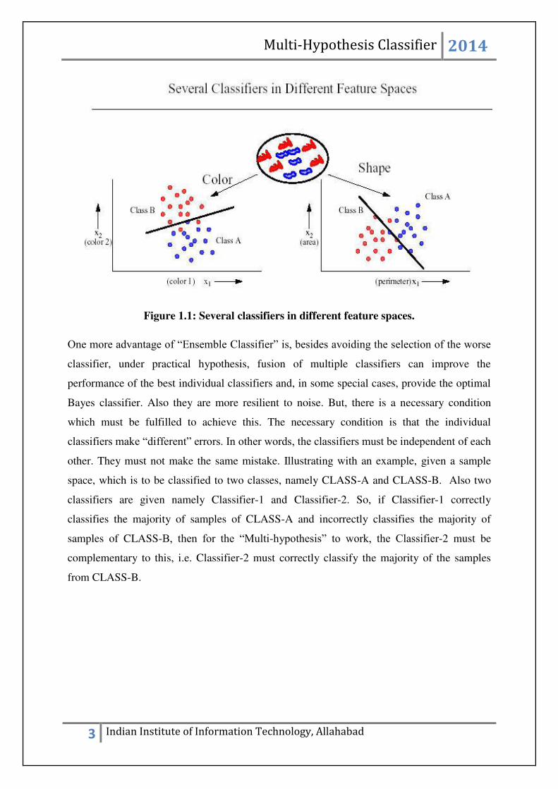
Figure 1.1 Several classifiers in different feature spaces.........……………………………. 3
Figure 1.2 Representation of the dilemma of several experts to reach a consensus..…….. 4
Figure 1.3 Representation of the best performing classifier...…………………………….. 5
Figure 1.4 Representation of the path followed by a classifier to local optima.…………… 5
Figure 1.5 Banana Data set............................................…………………………………… 6
Figure 1.6 Serial Architecture......................................................................………………… 7
Figure 1.7 Parallel Architecture..................................……………………………………..... 8
Figure 1.8 Hybrid Architecture......................................... ………………………………..… 8
Figure 1.9 Single feature set, different classifiers………..…………………......................... 9
Figure 1.10 Different feature space ..........……………………………………….......……… 10
Figure 1.11 Trained Combiners........……………………...………………………………… 11
Figure 2.1 Flowchart of Boosting................................……………………………………. 13
Figure 2.2 Data sampling in subsequent rounds of boosting............................…………… 14
Figure 2.3 Flowchart of Bagging..........................................................…………………… 16
Figure 3.1 Representation of the method of implementation of classifier #2........................ 42
Figure 3.2 A visual representation of 2-D Gabor Filter...………………………………….. 44
Figure 3.3 Gabor filter bank with different orientations applied on Chinese characters.….. 45
Figure 3.4 Regression v/s. PCA….............................................................................……… 46
Figure 4.1 Confusion matrix of classifier #1.....………………………………………….. 50
Figure 4.2 Confusion matrix of classifier #2…….....…………………………………….. 51
Figure 4.3 Confusion matrix of classifier #3………….....……………………………….. 54
Figure 4.4 Confidence Matrix………………………............................…………....…….. 55
Figure 4.5 Summary of Hypothesis #1…..............……………………………………….. 56
Figure 4.6 Confidence of samples from Hypothesis #2.....……………………………….. 63
Figure 4.7 Summary of Hypothesis #2..............………………………………………….. 66
Figure 4.8 Confusion matrix of classifier #1…………………..............…………………. 69
Figure 4.9 Confusion matrix of classifier #2....................................................…………… 70
Figure 4.10 Confusion matrix of classifier #3........................................…………………… 71
Figure 4.11 Confidence Matrix of hypothesis #3..................................................................... 72
xi
Figure 4.12 Summary of Hypothesis #3...……….........................………………………….. 73
Figure 4.13 Confusion matrix of classifier #1.….................................................................... 78
Figure 4.14 Confusion matrix of classifier #2.............................................................……… 79
Figure 4.15 Confusion matrix of classifier #3.....………………………………………….. 80
Figure 4.16 Confidence Matrix of Hypothesis #4....……........................…...…………….. 81
Figure 4.17 Summary of Hypothesis #4………….....…..........……………...…………….. 84
Figure 4.18 Summary of Hypothesis #5…………...........................…………...........…….. 87
List of Tables
Table 2.1 Data sampling in bagging and boosting..................…………………………… 16
Table 3.1 Overview of the data distribution.................................……………………….. 34
Table 3.2 Data distribution for classes with samples greater than 25…......…………….. 36
Table 3.3 Data distribution from different books for each class....………………….......…37
Table 3.4 Visual appearance of the data set..........……………………………………….. 39
Table 4.1 Number of components retained v/s accuracy......…………………………….. 52
Table 4.2 Size of Gabor kernel v/s accuracy………....………………………………….. 53
Table 5.1 Comparison of different hypotheses………………………………………….. 92

Multi-Hypothesis Classifier 2014
1 Indian Institute of Information Technology, Allahabad
Chapter 1
Introduction
1.1 Overview
Accuracy is the most important parameter among few others which defines the effectiveness
of a machine learning algorithm. Higher accuracy is always desirable. Now, there is a vast
number of well established learning algorithms already present in the scientific domain. Each
one of them has its own merits and demerits. Merits and demerits are evaluated in terms of
accuracy, speed of convergence, complexity of the algorithm, generalisation property, and
robustness among many others. Also the learning algorithms are data-distribution dependent.
Each learning algorithm is suitable for a particular distribution of data. Unfortunately, no
dominant classifier exists for all the data distribution, and the data distribution task at hand is
usually unknown. Not one classifier can be discriminative well enough if the number of
classes are huge. So the underlying problem is that a single classifier is not enough to classify
the whole sample space correctly. Before we dive deep in to the topic, we go through the
definition of “classifier”.
Classifier: A “Classifier” is any mapping from the space of features (measurements) to a
space of class labels (names, tags). A classifier is hypothesis about the real relation between
features and class labels. A “learning algorithm” is a method to construct hypotheses. A
learning algorithm applied to a set of samples (training set) outputs a classifier.
1.1.1 Rationale
In any application, we can use several learning algorithms. We can try many and
choose the one with the best cross-validation results. On the other hand, each learning
model comes with a set of assumption and thus bias. Learning is an ill-posed problem
(finite data), each model converges to a different solution and fails under different
circumstances. Why do not we combine multiple learners intelligently, which may

Multi-Hypothesis Classifier 2014
2 Indian Institute of Information Technology, Allahabad
lead to improved results? Now having said all this, the next question on our mind is Is
it really going to work? If yes, then Why? What is the rationale behind it?
1.1.2 Why it Works?
Assume that we have 25 base classifiers. Each of the 25 base classifiers has an error
rate, ε=0.35(say). Now if the base classifiers are identical, then the same examples
will be misclassified by the ensemble as incorrectly predicted by the base classifiers.
Assume classifiers are independent. The wrong prediction will be made only if more
than half of the base classifiers are wrong in their prediction. Probability that the
ensemble classifier makes a wrong prediction is 06.0*25
)1(25
25
13
ii
i i. See
the significant decrease in the error. The base classifiers should be chosen such that it
does better than a random guessing. Although, it is very hard to have classifiers
perfectly independent of each other.
One important point to be noted:
When multiple base learners are generated, it is not required for the individual classifiers to
be very accurate, so it is not necessary for them to be optimised separately. The base learners
are chosen for their simplicity, not for their accuracy.
1.2 Motivation
Why do we need multiple classifiers?
Now having gone through the definition of “classifier”, the question arises is what can be the
solution for this limitation of having single classifier? Is there a way, by which we can use
the positive points (discriminating features) of the individual classifier to achieve an overall
higher accuracy than the best accuracy obtained by a single learning algorithm? The solution
is “Ensemble Classifiers” which make use of the discriminating abilities of the individual
classifiers and fuses them together. Having said this, now many questions arise about the
techniques, methodologies, guarantee of accuracy of the fusion strategies. These issues would
be discussed in the following pages.
Multi-Hypothesis Classifier 2014
3 Indian Institute of Information Technology, Allahabad
Figure 1.1: Several classifiers in different feature spaces.
One more advantage of “Ensemble Classifier” is, besides avoiding the selection of the worse
classifier, under practical hypothesis, fusion of multiple classifiers can improve the
performance of the best individual classifiers and, in some special cases, provide the optimal
Bayes classifier. Also they are more resilient to noise. But, there is a necessary condition
which must be fulfilled to achieve this. The necessary condition is that the individual
classifiers make “different” errors. In other words, the classifiers must be independent of each
other. They must not make the same mistake. Illustrating with an example, given a sample
space, which is to be classified to two classes, namely CLASS-A and CLASS-B. Also two
classifiers are given namely Classifier-1 and Classifier-2. So, if Classifier-1 correctly
classifies the majority of samples of CLASS-A and incorrectly classifies the majority of
samples of CLASS-B, then for the “Multi-hypothesis” to work, the Classifier-2 must be
complementary to this, i.e. Classifier-2 must correctly classify the majority of the samples
from CLASS-B.

Multi-Hypothesis Classifier 2014
4 Indian Institute of Information Technology, Allahabad
Figure 1.2: Representation of the dilemma of several experts to reach a consensus.
There are many advantages to an ensemble of classifiers. Three main reasons on why a
classifier ensemble might be better than single classifier [1].
1.3 Reasons for the usefulness of ensemble classifier
1.3.1 Statistical
Let us assume that there are a number of classifiers with a decent performance on a
given labelled dataset as shown in Figure 1.1. Generalisation performance is
different on the data for each of the classifiers. There is always a choice to pick a
single classifier for solution, which may lead to a bad decision. A better choice
would be to use multiple classifiers and ‘average’ their outputs. The new ensemble
classifier may not improve the results from the best individual classifier but will
eliminate the risk of picking an insufficient single classifier.

Multi-Hypothesis Classifier 2014
5 Indian Institute of Information Technology, Allahabad
Figure 1.3: D* is the best performing individual classifier; the space of all
classifiers is depicted as the outer curve; the shaded area depicts the space of
good performance classifiers.
1.3.2 Computational
Some of the learning algorithms perform hill-climbing or random search, which has
a great chance to lead to a local optima as shown in Figure 1.2.
Figure 1.4: D* is the best classifier for the data; the space of all classifiers is
shown by the outer curve; the dashed lines represents the hypothetical path or
trajectories for the classifiers during training.
Multi-Hypothesis Classifier 2014
6 Indian Institute of Information Technology, Allahabad
We go with the assumption that the training process of each classifier starts
somewhere in the space of possible classifiers and terminates closer to the optimal
classifier D*. So some form of mixing or aggregating may lead to classifier that is a
better approximation to D* than any single classifier Di.
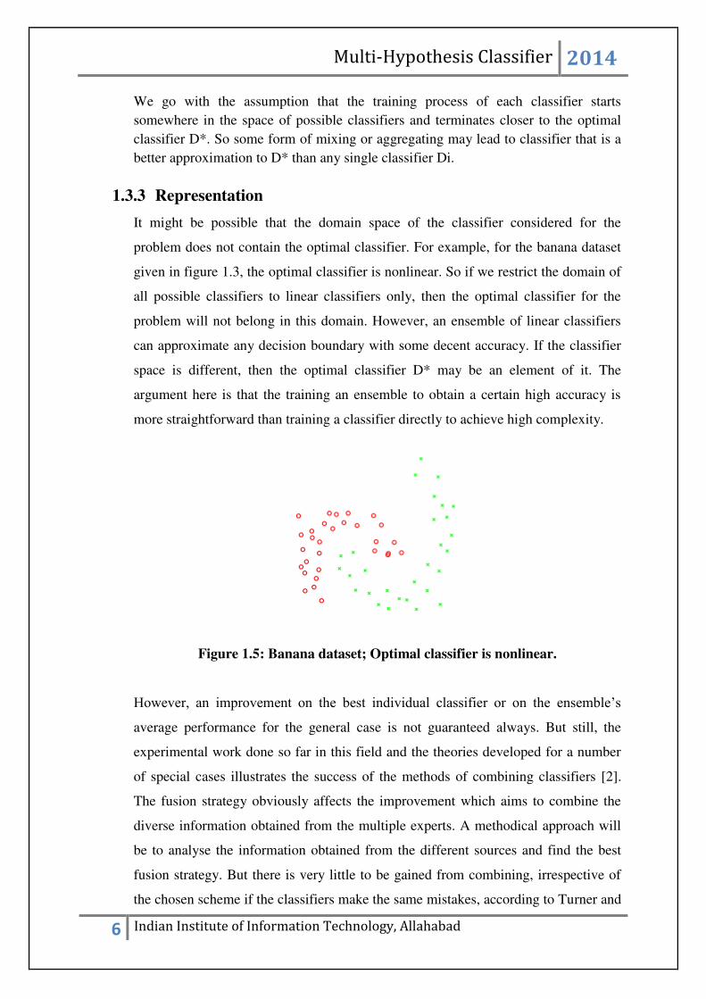
1.3.3 Representation
It might be possible that the domain space of the classifier considered for the
problem does not contain the optimal classifier. For example, for the banana dataset
given in figure 1.3, the optimal classifier is nonlinear. So if we restrict the domain of
all possible classifiers to linear classifiers only, then the optimal classifier for the
problem will not belong in this domain. However, an ensemble of linear classifiers
can approximate any decision boundary with some decent accuracy. If the classifier
space is different, then the optimal classifier D* may be an element of it. The
argument here is that the training an ensemble to obtain a certain high accuracy is
more straightforward than training a classifier directly to achieve high complexity.
Figure 1.5: Banana dataset; Optimal classifier is nonlinear.
However, an improvement on the best individual classifier or on the ensemble’s
average performance for the general case is not guaranteed always. But still, the
experimental work done so far in this field and the theories developed for a number
of special cases illustrates the success of the methods of combining classifiers [2].
The fusion strategy obviously affects the improvement which aims to combine the
diverse information obtained from the multiple experts. A methodical approach will
be to analyse the information obtained from the different sources and find the best
fusion strategy. But there is very little to be gained from combining, irrespective of
the chosen scheme if the classifiers make the same mistakes, according to Turner and

Multi-Hypothesis Classifier 2014
7 Indian Institute of Information Technology, Allahabad
Ghosh [3]. In many cases we have the flexibility to create multiple classifiers. In
such scenarios, we can select a fusion strategy and then a set of multiple classifiers
can be formed which contains the diverse information which helps in increasing the
accuracy.
1.4 Multiple Classifier System (MCS)
A multiple classifier system (MCS) is a structured way to combine (exploit) the
outputs of individual classifiers. MCS can be thought as multiple expert systems,
committees of experts, mixtures of experts, classifier ensembles, and composite
classifier systems. Multiple classifier system (MCS) can be characterized by:
The Architecture
Fixed/Trained Combination strategy
Others
1.4.1 MCS Architecture/Topology
1.4.1.1 Serial
Figure 1.6: Serial architecture.
EXPERT 1
EXPERT 2
.................
EXPERT N

Multi-Hypothesis Classifier 2014
8 Indian Institute of Information Technology, Allahabad
1.4.1.2 Parallel
Figure 1.7: Parallel architecture.
1.4.1.3 Hybrid
Figure 1.8: Hybrid architecture.
EXPERT 1 EXPERT 2 ............
EXPERT N
Combining Strategy
EXPERT 1
EXPERT 2
EXPERT N
COMBINER 1
COMBINER 2
..............

Multi-Hypothesis Classifier 2014
9 Indian Institute of Information Technology, Allahabad
Now, having gone through the basic architectures for multiple classifier systems, the
next logical question arise is, what are the multiple classifier source? Sources can be
differentiated based on,
1 Different Feature spaces (Face, voice, fingerprint)
2 Different Training sets (Sampling, Boosting, Bagging)
3 Different Classifiers (KNN,ANN,SVM)
4 Different Architectures (Neural Net: layers, Units, Transfer function)
5 Different parameter values ( k in kNN, Kernel in SVM)
6 Different initialisations
Combination based on a single space but different classifiers
Figure 1.9: Single feature set, different classifiers.
Multi-Hypothesis Classifier 2014
10 Indian Institute of Information Technology, Allahabad
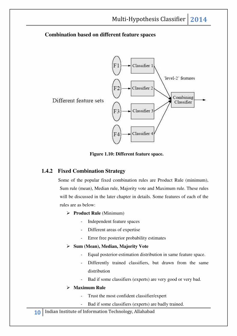
Combination based on different feature spaces
Figure 1.10: Different feature space.
1.4.2 Fixed Combination Strategy
Some of the popular fixed combination rules are Product Rule (minimum),
Sum rule (mean), Median rule, Majority vote and Maximum rule. These rules
will be discussed in the later chapter in details. Some features of each of the
rules are as below:
Product Rule (Minimum)
- Independent feature spaces
- Different areas of expertise
- Error free posterior probability estimates
Sum (Mean), Median, Majority Vote
- Equal posterior-estimation distribution in same feature space.
- Differently trained classifiers, but drawn from the same
distribution
- Bad if some classifiers (experts) are very good or very bad.
Maximum Rule
- Trust the most confident classifier/expert
- Bad if some classifiers (experts) are badly trained.
Multi-Hypothesis Classifier 2014
11 Indian Institute of Information Technology, Allahabad
Having listed the above rules, one important factor which put it in disadvantage than the
trained combiner is that the fixed combining rules are sub-optimal. Base classifiers are never
really independent (Product Rule).Base classifiers are never really equally imperfectly trained
(sum, median, majority vote). Also the sensitivity to over-confident base classifiers (Product,
min, max). This leads to the emergence of the emergence of the trained combiners.
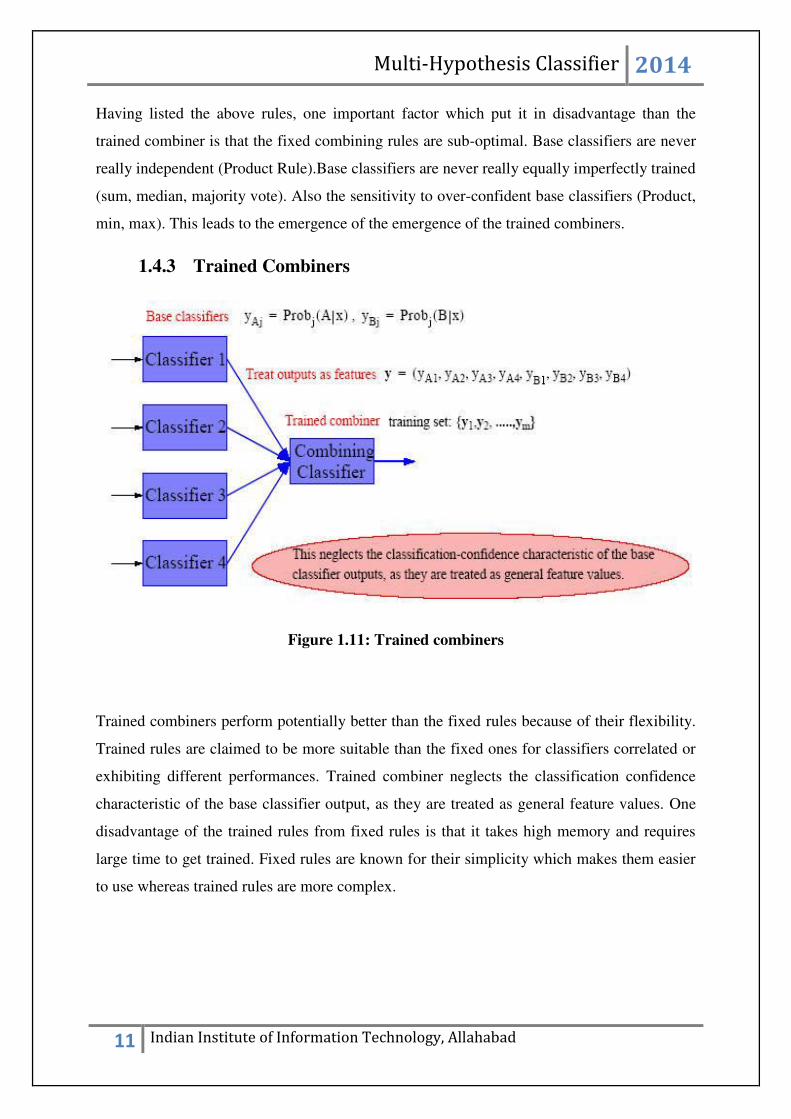
1.4.3 Trained Combiners
Figure 1.11: Trained combiners
Trained combiners perform potentially better than the fixed rules because of their flexibility.
Trained rules are claimed to be more suitable than the fixed ones for classifiers correlated or
exhibiting different performances. Trained combiner neglects the classification confidence
characteristic of the base classifier output, as they are treated as general feature values. One
disadvantage of the trained rules from fixed rules is that it takes high memory and requires
large time to get trained. Fixed rules are known for their simplicity which makes them easier
to use whereas trained rules are more complex.

Multi-Hypothesis Classifier 2014
12 Indian Institute of Information Technology, Allahabad
Chapter 2
Literature Survey
What has already been done?
2.1 Boosting
Boosting is a old effective way to combine classifiers. It was introduced by
Schapire and Freund in 1990s. Boosting convert a weak learning algorithm into a
strong one. Having said that, the analogy is still not clear. Let me summarize how
the pioneers of this field Freund and Schapire approached the understanding of
this method.
2.1.1 Analogy: “There was a gambler, who was frustrated by the non-stop losses
in the horse racing and was jealous of his friend’s success in the same events. Not
being able to find out the reason behind his failure, he allows his group of best
pals cum gamblers to make bets on his behalf. He makes up his mind that he will
wager a fixed sum of money in every race. But there was also a catch. He decides
that he will proportionally divide his money among his friends depending on how
well they are performing. Certainly, if he knew psychically beforehand which of
his friend would win the most, he would obviously have that friend handle all his
wagers. But due to the lack of such clear vision, he allocates each race’s wager in
such a way that his total earning for the whole season will be reasonably close to
what he would have won had he bet on his luckiest friend . This method is all
about dynamic allocation problem.
Now suppose the gambler gets tired of choosing among the experts and instead
he would like to create a computer program which would predict the winner of
the race using some usual information (races won by individual horses, betting
odds, etc.). To create this sort of a program, he asks all his experts to articulate
their strategy. Not surprisingly, the experts are unable to come up with a grand
set of rules for selecting a horse. On the other hand they were able to come up

Multi-Hypothesis Classifier 2014
13 Indian Institute of Information Technology, Allahabad
with a solution when presented data for a specific set of races. Such rules of
thumbs (horse with most favoured odds) are usually very inaccurate and rough.
They are expected to give results which might be slightly better than random
guessing, which will not be unreasonable to expect. By asking the experts their
opinion again and again on different collection of races, the gambler is able to
gather many rules-of-thumb”.
Now in order to use these rules to maximum advantage, there arise two issues.
First, how must he choose the collection of races presented to the expert so as to
extract the most useful rules of thumb from the expert? Second, how can the
rules be combined to form a single highly effective and accurate rule, once he has
collected many rules-of-thumb? Boosting provides the combination technique to
for accurate prediction for moderately inaccurate rules-of-thumb.
Figure 2.1: Flowchart of Boosting.
Now, having established the analogy lets dive in to the technical know-how of
this method. The main idea is to combine many weak classifiers to produce
powerful committee. So the classifiers are produced sequentially, one after the
other. Each classifier is dependent on the previous one, and focuses on the
previous one’s errors. Examples that are incorrectly predicted in the previous
classifiers are chosen more often or weighted more heavily. Records that are

Multi-Hypothesis Classifier 2014
14 Indian Institute of Information Technology, Allahabad
wrongly classified will have their weights increased. Records that are classified
correctly will have their weights decreased. Given an example below,
Figure 2.2: Example of data sampling in subsequent rounds of boosting.
As we can see from the above table that, example 4 is hard to classify. So its
weight is increased, therefore it is more likely to be chosen again in the
subsequent rounds. Boosting algorithm differs in terms of (1) how the weights of
the training examples are updated at the end of each round, and (2) how the
predictions made by each classifier are combined.
2.1.2 The basic Ada-Boosting Algorithm
For t=1 . . . , T
Train weak learner using training data and d t.
Get ht: X {-1,1} with error
yixihti
ttiD
)(:
)(
Choose t
t
t
1ln
2
1
Update eZ
DD
t
t
t
t
ii
*
)()(
1 if yxh iit
)(
eZ
DD
t
t
t
t
ii
*
)()(
1 if yxh iit
)(
= eZ
D xhyiitit
t
t )()( , (2.1)
Where Z t is the normalisation factor (chosen so that Dt 1
will be a
distribution).
Original Data 1 2 3 4 5 6 7 8 9 10
Boosting (Round 1) 7 3 2 8 7 9 4 10 6 3
Boosting (Round 2) 5 4 9 4 2 5 1 7 4 2
Boosting (Round 3) 4 4 8 10 4 5 4 6 3 4

Multi-Hypothesis Classifier 2014
15 Indian Institute of Information Technology, Allahabad
The hypothesis weight t is decided at round t. The weight
distribution of training examples is updated at every round t. But
Boosting comes with its own sets of issues. The main issues are-
Givenht, how to choose t
?
How to selectht?
How to deal with multi-class problems?
2.1.3 Strengths of Ada-boost
It has no parameters to tune (except for the number of rounds)
It is fast, simple and easy to program
It comes with a set of theoretical guarantee (training error, test error)
Instead of designing a learning algorithm that is accurate over the entire space, we can
focus on finding the base learning algorithms that only need to be better than random.
It can identify outliners i.e. examples that are either mislabelled or that are inherently
ambiguous and hard to categorize.
2.1.4 Weakness of Ada-Boost
The actual performance of boosting depends on the data and the base learner.
Boosting seems to be especially susceptible to noise.
When the number of outliners is very large, the emphasis placed on the hard examples
can hurt the performance.
2.2 Bagging
Introduced by Breiman[4]. Derived from bootstrap (Efron,1993). It creates classifiers
using training sets that are bootstrapped (drawn with replacement).Each bootstrap sample
D has the same size as the original data. Some instances could appear several times in the
training set, while others may be omitted. The idea is to build classifier on each bootstrap
sample D. D will contain approximately 63% of the original data. Each data object has
Multi-Hypothesis Classifier 2014
16 Indian Institute of Information Technology, Allahabad
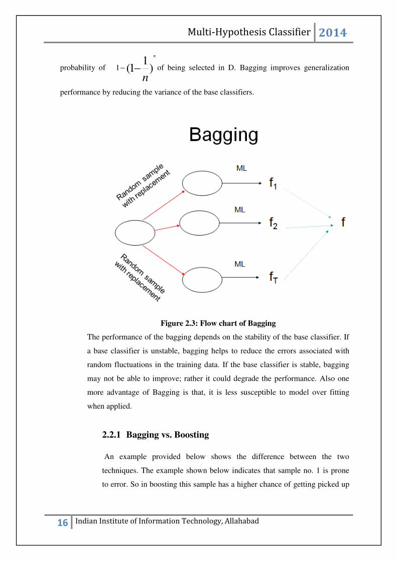
probability of )1
1(1
n
n
of being selected in D. Bagging improves generalization
performance by reducing the variance of the base classifiers.
Figure 2.3: Flow chart of Bagging
The performance of the bagging depends on the stability of the base classifier. If
a base classifier is unstable, bagging helps to reduce the errors associated with
random fluctuations in the training data. If the base classifier is stable, bagging
may not be able to improve; rather it could degrade the performance. Also one
more advantage of Bagging is that, it is less susceptible to model over fitting
when applied.
2.2.1 Bagging vs. Boosting
An example provided below shows the difference between the two
techniques. The example shown below indicates that sample no. 1 is prone
to error. So in boosting this sample has a higher chance of getting picked up

Multi-Hypothesis Classifier 2014
17 Indian Institute of Information Technology, Allahabad
in the set. Whereas in bagging, the sampling is independent of the previous
set.
Training Data
1 , 2 , 3 , 4 , 5 , 6 , 7 , 8
Bagging Training set Boosting Training set
Set 1: 2, 7, 8, 3, 7, 6, 3, 1
Set 2: 7, 8, 5, 6, 4, 2, 7, 1
Set 3: 3, 6, 2, 7, 5, 6, 2, 2
Set 4: 4, 5, 1, 4, 6, 4, 3, 8
Set 1: 2, 7, 8, 3, 7, 6, 3, 1
Set 2: 1, 4, 5, 4, 1, 5, 6, 4
Set 3: 7, 1, 5, 8, 1, 8, 1, 4
Set 4: 1, 1, 6, 1, 1, 3, 1, 5
Table 2.1: Training set (above); Data sampling in bagging and boosting.
Some important conclusions from the above two techniques:
- Bagging always uses re-sampling rather than re-weighting.
- Bagging does not modify the distribution over examples or mislabels, but instead
always uses the uniform distribution.
- In forming the final hypothesis, bagging gives equal weight to each of the weak
hypotheses.
Experimental Results on Ensembles (Freund and Schapire, 1996; Quinlan, 1996) [5]:
- Ensembles improve generalization accuracy on a wide variety of problems.
- On average, Boosting provides a larger increase in accuracy than Bagging.
- Boosting on rare occasion can degrade accuracy.
- Bagging more consistently provides a modest improvement.
- Boosting is particularly subject to over-fitting when there is significant noise in the
training data.
2.3 Issues in Ensembles
- Parallelism in ensembles: Bagging is easily parallelized whereas Boosting is not.
- How “weak” should a base learner for Boosting be?
- Variants of Boosting to handle noisy data.
- What is the theoretical explanation of Boosting’s ability to improve generalization?

Multi-Hypothesis Classifier 2014
18 Indian Institute of Information Technology, Allahabad
- Exactly how does the diversity of ensembles affect their ensemble performance?
- Combining Boosting and Bagging.
The above two techniques exploits the fact that multiple training set leads to the formation of
multiple classifiers. Instead we can design multiple classifiers with the same dataset. Now
broadly there are two large groups of methods of classification, (1) Feature Vector based
methods and (2) Structural and Syntactic methods. Also each group again includes different
algorithms based on different methodologies. For the first group itself, there exists k-NN
classifier, Bayes classifier, neural network based classifiers and various distance based
classifiers among others. So there is a big challenge to devise an effective
strategy/methodology to combine the outputs of all the different breeds of classifiers which
outputs different levels of information. Also how to obtain a consensus on the result of each
individual classifier?
Methods for fusing classifiers can be differentiated according to the type of information
produced by the individual classifiers [7]. They are:
- Abstract level: A classifier only outputs a unique label for each input pattern.
- Rank level: Each classifier outputs a list of possible classes, with ranking for each
input pattern.
- Measurement level: Each classifier outputs class confidence levels for each input
pattern.
For each of the above categories, methods can be further subdivided into Integration vs.
Selection rules and Fixed rules vs. trained rules. Example of a fixed rule at abstract-level
is the majority voting rule.
Next we talk about Fuser (Combination rule). Broadly, fuser can be classified into two
main categories:
- Integration (fusion) function: For each pattern, all the classifiers contribute to
the final decision. Integration assumes competitive classifiers.
- Selection functions: For each pattern, just one classifier, or a subset, is
responsible for the final decision. Selection assumes complementary classifiers.
Integration and selection can be merged for designing the hybrid fuser. For this, multiple
functions for non-parallel architecture can be necessary.

Multi-Hypothesis Classifier 2014
19 Indian Institute of Information Technology, Allahabad
2.3.1 Diversity in Classifiers
Next we talk briefly about classifier’s diversity. Measure of diversity in classifier ensembles
are a matter of ongoing research (L. I. Kuncheva). The key issue in this domain is: How are
the diversity measures related to the accuracy of the ensembles?
Fusion is obviously useful only if the combined classifiers are mutually complementary
(ideally, classifiers with and high diversity high accuracy). The required degree of error
diversity depends on the fuser complexity. An example, the whole can be divided in to four
diversity levels (A. Sharkey,1999) [11].
- Level 1: No more than one classifier is wrong for each pattern.
- Level 2: The majority is always correct.
- Level 3: At least one classifier is correct for each pattern.
- Level 4: All classifiers are wrong for some pattern.
Simple fusers can be used for classifiers that exhibit a simple complementary pattern (e.g.
majority voting). Complex fusers, for example, a dynamic selector, are necessary for
classifiers with a complex dependency model. The required complexity of the fuser depends
on the degree of classifier’s diversity.
The design of MCS (Multiple classifier systems) involves two main phases, (1) The design of
the classifier ensemble, and (2) The design of the fuser. The design of the classifier ensemble
is aimed to create a set of complementary/diverse classifiers. On the other hand, the design of
the combination function/fuser is aimed to create a fusion mechanism that can exploit the
complementary/diversity of the classifiers and optimally combine them. The above two
phases are obviously linked. In this thesis, we focus more on the second phase i.e. design of
the fuser.
2.4 Average Bayes Classifier and its versions
This section deals with the combination problem where the output from each classifier
is available in measurement level. First, we consider that all classifiers are Bayes
classifiers. For a Bayes classifier e, the classification is based actually on a real set of
measurements-post probabilities:
MixxP Ci,........,1),(
(2.2)

Multi-Hypothesis Classifier 2014
20 Indian Institute of Information Technology, Allahabad
Where sample x comes from class Ci. These probabilities are not related to
individual classifier Ek. In practice, each classifier classifies a sample to a
particular class is not really based on the true values of the above equation, which
are not available. For each sample x, a set of approximations are estimated by
classifier Ek itself. These approximations are based on what features the
classifier is used on and how the classifiers are trained. To clarify such
dependence, we denote it as follows:
.,.....,1,,.....,1),( KkMixx CP ik
(2.3)
The above equation gives the approximation for combining the classification
results on the same sample by all the K classifiers. One simple approach given by
Lei Xu (1992) [ ], calls for a little modification in the above approach. They use
the following average value as a new estimation of the combined classifier:
MixxK
xxK
kikiE CPCP ,.....,1),(
1)(
1
(2.4)
The final decision made by the classifier E is given by:
E(x) = j, with )(max)( xxxx CPCP iEijE
(2.5)
The above Bayes decision is based on the newly estimated post-probabilities.
Such a combined classifier is called as an Averaged Bayes classifier. The above
approach could as well be extended to cover several cases where there are
different kinds of classifiers. Generally, any classifiers where some kinds of post
probabilities are computable could be combined by means of equation (2.5).

Multi-Hypothesis Classifier 2014
21 Indian Institute of Information Technology, Allahabad
2.5 Combining Multiple Classifiers using Voting Principle and its
variants [8]
It may so happen that the individual classifier does not agree on a particular
sample about which class it belongs to. A simple rule used for resolving this kind
of disputes in human social life is by majority voting. Now, the basic principle
can be altered/modified a bit to bring out the variants which may be suitable
under certain conditions. First, for our convenience, let us represent the event
ixek)( in a binary characteristic function form.
1)( CT ikx , when ixek
)( and i (2.6)
0)( CT ikx , otherwise.
The most conservative voting rule is the following:
jxE )( , if 0)(1
CT jk
K
kxj
(2.7)
1)( MxE , Otherwise
The above equation means that if all K classifiers decide that sample x belongs to
class C j unanimously, then classifier E decides that x comes from C j
,
otherwise it rejects x. In the above equation denotes the logical AND operator
or binary multiplication and in the following equations denotes the logical OR
operator or binary summation.
A slight altering of the above equation will lead to a version which is less rigid as
shown below.
jxE )( , if 0)}(1()({11
CTCT qK
M
qjk
K
kxxj
(2.8)
1)( MxE , Otherwise
Multi-Hypothesis Classifier 2014
22 Indian Institute of Information Technology, Allahabad
The above modified equation, means that sample x belongs to a particular class
C kas long as some of the classifiers support that class C k
and no other
classifier support a different class. In other words, the classifiers that reject the
sample x will have no impact on the combined classifier unless all the classifier
reject x.
Now for a case, where there are more than two labels that receive the maximal
votes or the maximum vote obtained is not much larger than the second
maximum votes. In such cases, even if the vote received by a label is large, but
there is equally another large vote which goes against the first label. To tackle
this problem, a new kind of majority voting is proposed below:
jxE )( , max1)( CT jE
x and K*maxmax 21
(2.9)
1)( MxE , Otherwise
Where 0 < α <= 1. As the number of classifiers (K) are constant. The vote of the
second maximum is taken as the implicit objections to the label j.
2.6 Combination of Classifiers in Dempster-Shafer Formalism
This combination technique is useful only when the output information provided
by each classifier is in abstract form, i.e. only class label information is provided
as output. As a prior knowledge, only the substitution, recognition and rejection
rates of each classifier are used.
2.6.1 Dempster-Shafer Theory [9, 10]:
Let me first give the key points of this theory. Given a number of exhaustive and
mutually exclusive propositions ,,.....,1, MiAi of the universal set
AA M,......,
1 . Any subset AA iqi
,.....,1
is a proposition denoting the
disjunction AA iqi ......
1. Each element Ai
called a singleton which
corresponds to a one element subset. All subsets possible of forms a superset
2
. The Dempster-Shafer theory uses a value in the range of 0 and 1, inclusive
Multi-Hypothesis Classifier 2014
23 Indian Institute of Information Technology, Allahabad
to give a belief in a proposition, given the occurrence of some evidence e. It is
denoted as bel(A), gives information about the degree to which the evidence e
supports the proposition A. The belief function bel(A) is calculated from another
function which is known as the Basic Probability Assignment(BPA). This
function gives information about the individual impact of each evidences on our
propositions. The BPA is denoted by m, and can also be generalized as
probability mass distribution. It assigns numeric values in the closed range of 0
and 1 to each subset of i.e. every element of2
, such that the values sum up
to 1. Three distinct features about BPA:
- m(A) is just a small part of the total belief assigned exactly to A. It can’t
be subdivided among the subsets of A.
- The singletons are only some of the part of the whole elements of the
superset2
. So it is quite possible that 11
M
i iAm , and also Ai and
Ai are the sole two elements of the superset 2
, so the relation
1 AA iimm holds true. This violates the basic axioms of
Bayesian theory. So the BPA provides an incomplete probabilistic model.
- A subset A of the superset 2
with m(A)>0 is called a focal element.
When there is only one focal element in the superset, then m( ) absorbs
the unassigned part of the total belief. m( ) = 1 – m(A).
Now as subset A is the disjunction of all elements in A, if BA, then the
truth of B implies the truth of A. Hence, the belief function bel(A) is given
by,
AB
BmAbel )()(
(2.10)
If more than two evidences exists, two or more sets of BPA’s and bel(.. )’s
will be applied to the same subset of . If m1, m2
and bel1,bel2
denote
the two BPA’s and their corresponding belief functions respectively, then the
D-S rule defines a new BPA given by mmm 21 , which gives the
combined effect of both m1 and m2
, i.e. for A is not equal to an empty set:

Multi-Hypothesis Classifier 2014
24 Indian Institute of Information Technology, Allahabad
YXkAAm mmmmAAYX
2.
121
(2.11)
Where,
)()()()(12121
1YXYX mmmmk
YXYX
(2.12)
The necessary condition for the BPA to exist is : 01
k . If 01
k , then
the two evidences are said to be in conflict, i,e. They are in total
contradiction. mm 21 does not exists. If there is no contradiction, then the
overall belief function bel(A) can be calculated from the result of the
combined BPA.
2.6.2 Modelling Multi classifier combination using Dempster-
Shafer Theory
In this problem, the M mutually exclusive and exhaustive propositions are
given by ix CA i,
1which denotes that sample x comes from class
label C i. The universal proposition is AA M
,......,1
. There are K
classifiers ee K,.....,
1 which will give K evidences,
Kkx je kk,......,2,1,)( with each evidence denoting that sample x is
assigned a class label by classifiereK.
We have prior knowledge of the recognition rate )(k
r and the substitution
rate )(k
s of eK
. For each evidences produced je kkx , one could infer
uncertain beliefs that the proposition CA jkjkx is true with a degree
)(k
r(recognition rate) and is not true with a degree )(k
s. If x is rejected by
eKi.e. when 1 Mj
k, it has no idea of the any given propositions, and it
infers the full support of the universal proposition . Now we can define a

Multi-Hypothesis Classifier 2014
25 Indian Institute of Information Technology, Allahabad
Basic Probability Assignment function mkon the universal proposition for
evidence in the given way:
- mkhas only one focal element , when 1 Mj
k, with
1)( mk.This is a degenerated case as the evidence eK
says
nothing about the any of the M propositions.
- If jk
, only two focal elements are there in mk, namely A jk
and
AA jkjk . Now we have )(k
rjkk Am and
)(k
sjkk Am . As eK says nothing about other propositions, we
have )()(1)(
k
s
k
rkm . As we have K evidences, we will
obtain K basic probability assignment functions Kkmk...,1, . Now
as we have formulated the problem in a usable format, the next step is
to use the D-S rule to obtain a combined BPA
mmmmm K .......
321 and use this new BPA to
calculate the belief functions Aibel and Ai
bel based on the K
evidences we gathered. After this the combined classifier could be
formed by using the decision rules derived from these beliefs.
2.6.3 Conclusion of D-S Theory
Now having concluded the above section, we have seen three
approaches namely Bayesian Formalism, Voting principle and
Dempster Shafer theory. Let us summarize the comparative
advantages/disadvantages of each over one another.
- We found out that the D-S approach is quite robust. Inaccurate
learning doesn’t affect the performance much [9].
- If the confusion matrix of each algorithm is well learned, then
Bayesian approach is the best method. Although it is unstable.
Rough learning will degrade the performance quickly [9].

Multi-Hypothesis Classifier 2014
26 Indian Institute of Information Technology, Allahabad
- The D-S approach is better than the voting approach when high
reliability is required [9].
2.7 Some fixed rules of combination [8]:
There are broadly two combination scenarios. In the first scenario, the classifiers use the
same representation of the input pattern. An example being a set of k-NN classifiers, each
using the same measurement vectors, but classifier parameters are different (k varies, distance
metrics varies). When given an input pattern, this produces an estimate of the same a
posterior class probability. In the second scenario, the classifiers use their own representation
of the input pattern. The measurements extracted by each classifier from the pattern are
unique to each classifier. The combination of this type requires to physically integrate the
different types of measurement/features as the computed a posterior probabilities are not the
estimate of the same functional values. Kittler et al(1998), devise a framework which under
some assumptions can lead to a proper formulation of some commonly used combining
strategy.
2.7.1 Theoretical framework
Let us consider a pattern recognition problem, in which pattern Z is to be assigned to one of
the possible classes ww m,.......,
1. Also we have R classifiers each one representing the
pattern with a unique measurement vector. The measurement vector used by the ith classifier
is denoted by xi. The class wk
can be modelled by the PDF wx kip and its prior
probability of occurrence can be denoted as wkp . The models are assumed to be mutually
exclusive, i.e. each pattern is associated with only one model. Now according to the Bayesian
theory,
xx
wwxxxxw
R
kkR
Rk p
Ppp
,.......,
)(|,........,,........,
1
1
1
(2.13)
Where,

Multi-Hypothesis Classifier 2014
27 Indian Institute of Information Technology, Allahabad
wwxxxx j
m
jjRRPpp
1
11|,.....,,......,
(2.14)
2.7.2 Product Rule
The basic assumption made to arrive at the product rule is that the representations used are
conditionally independent. This consequence can be formulated as,
R
ikikR wxwxx pp
11
||,.....,
(2.15)
Now substituting the above equation in the previously obtained Bayes equation, we find
m
j
R
i jij
R
i kik
Rk
wxw
wxwxxw
pP
pPP
1 1
1
1|
|,......,|
(2.16)
And the decision rule formulated is,
Assign Z w j if
R
ikik
m
k
R
ijij wxwwxw PPpP
111
|| max (2.17)
Or in terms of the a posterior probabilities obtained by the respective classifiers
Assign Z w j if
R
iikk
Rm
k
R
iijj
R
xwwPxwwP PP1
)1(
11
)1(|max|
(2.18)
2.7.3 Sum Rule
To derive at the sum rule a strong assumption is made. It is assumed that the a posterior
probability computed by the respective classifiers will not deviate drastically much from the
prior probabilities. The sum decision rule can be denoted as,

Multi-Hypothesis Classifier 2014
28 Indian Institute of Information Technology, Allahabad
assign Z w j if
R
iikk
m
k
R
iijj xwwxww PPRPPR
11
1
|1max|1
(2.19)
Due to the assumption made, if the patterns convey discriminating information, the sum rule
will introduce gross approximation error.
The decision rules ( ) and ( ) lays the foundation for classifier combination. Other popular
combination schemes can be derived from these rules by noting that,
xwxwxwxw ik
R
i
R
iikik
R
i
R
iik
PPR
PP |max|1
|min|1
111
(2.20)
The above relationship suggests that the sum and the product combination rules can be
approximated by the above upper and lower bounds. The a posterior probabilities xw ikP |
can be hardened to produce binary valued function ki as
Otherwise
PPif xwxw ij
m
jik
ki
,.....0
|max|......,11
(2.21)
The above function, instead of combining a posteriori probabilities, combines decision
outcomes. The above approximations will lead to the following rules.
2.7.4 Max Rule
Using (2.20) and approximating the sum using the maximum of the posterior probabilities,
assign Z w j if
R
iikk
R
iij
R
ij xwwxww PRPRPRPR1
11|max1max|max1
(2.22)
Assuming the priors are equal, it simplifies to,

Multi-Hypothesis Classifier 2014
29 Indian Institute of Information Technology, Allahabad
assign Z w j if
xwxw ik
R
i
m
kij
R
iPP |maxmax|max
111
(2.23)
2.7.5 Min Rule
Using (2.18) and bounding the product of the posterior probabilities we obtain,
assign Z w j if
xwwPxwwP ik
R
ik
Rm
kij
R
ij
RPP |minmax|min
1
)1(
11
)1(
(2.24)
Assuming the priors are equal, it simplifies to
assign Z w j if
xwxw ik
R
i
m
kij
R
iPP |minmax|min
111
(2.25)
2.7.6 Mean Rule
The sum rule in (2.20), under the equal prior assumption can be viewed to be computing the
average a posterior probability over all the classifier outputs for each class, i.e.
assign Z w j if
R
iik
m
k
R
iij xwxw P
RP
R 11
1
|1
max|1
(2.26)
Thus the class with the maximum average a posterior probability get assigned to the pattern.

Multi-Hypothesis Classifier 2014
30 Indian Institute of Information Technology, Allahabad
2.7.7 Median Rule
Taking a clue from the above rule, in case of an outlier, the average posterior probability will
be affected, which in turn will lead to an incorrect decision. Also a popularly known fact is
that the median is a better or robust estimate of the mean. So it could be wise to model the
combined decision on the median of the a posterior probabilities.
assign Z w j if
xwxw ik
R
i
m
kij
R
iPmedPmed |max|
111
(2.27)

Multi-Hypothesis Classifier 2014
31 Indian Institute of Information Technology, Allahabad
Chapter 3
Proposed Methodology
In the earlier work done in the combination approaches, majority of the researchers have
played with weak classifiers. Common approach to form a weak classifier is by tweaking the
training data or by using different sampling techniques and feeding it to a learning algorithm.
Bagging and Boosting as discussed above are the examples of combining weak classifiers. In
my research, I have experimented with the combination of few strong classifiers. In all, three
classifiers are build, namely nearest neighbour on raw image pixels, Nearest neighbour on a
structural feature extracted image, and Nearest neighbour on GABOR feature extracted
image. PCA is also used after the GABOR feature extraction process due to the high
dimensionality and redundancy of the feature vector. The bank of GABOR filters used is
formed by using different orientation, kernel size and frequency of the filter. After the
classifiers are formed having their individual accuracy, now each classifier forms a
hypothesis. A hypothesis is a proposed explanation for a phenomenon. Each classifier gives
its own hypothesis in the form of a confusion matrix. My task is to use the relevant
information from each classifier and suggest a suitable framework and technique to combine
all the classifiers in such a way, which would take in to account the positive discriminating
features of each classifier and help to increase the overall accuracy of the ensemble better
than what is obtained by the individual classifiers. A confidence chart is prepared using the
confusion matrix or test sample accuracy which gives the confidence about the classifiers on
each class labels or on particular samples of data. Formation techniques of the confidence
chart lay the foundation of this whole research. There can be many techniques to form the
confidence chart (apart from using the information from the confusion matrix). Based on the
technique, corresponding hypotheses are proposed for the ensemble. In my research, I have
used 5 different hypotheses based on different ways of creating the confidence chart. To
combine the three classifiers, maximum rule and weighted majority voting rules are used and
analysed.
Multi-Hypothesis Classifier 2014
32 Indian Institute of Information Technology, Allahabad
Also the basic assumption still holds true, which is about the conditional independence of the
data i.e. the classifiers, will not make the same mistake. But there is no guarantee to it.
Although one can’t say for sure, how much the accuracy will increase, if at all it increases
due to the different ways of collecting the data and percolation of noise into it. But one thing
that can be said about the combination approaches are that, this will stabilise the accuracy to
a certain point, i.e individual accuracies might change when the data samples change, but an
effective combination strategy will ensure that the overall accuracy of the ensemble doesn’t
change drastically due to the dynamic nature of the data. This is one of the biggest
advantages of using an ensemble.
Before we dive deep, let us first have a look at the data set.
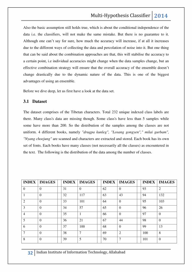
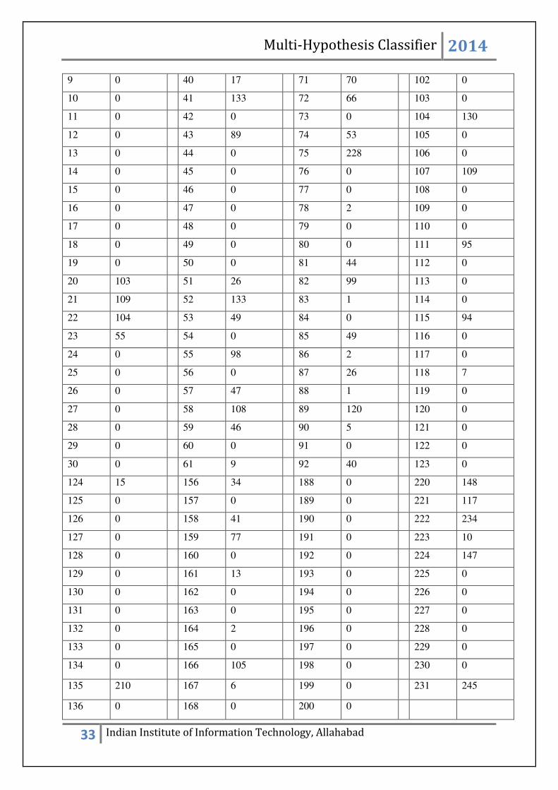
3.1 Dataset
The dataset comprises of the Tibetan characters. Total 232 unique indexed class labels are
there. Many class's data are missing though. Some class's have less than 5 samples while
some have more than 200. So the distribution of the samples among the classes are not
uniform. 4 different books, namely "drugpa kunleg", "Losang gongyen"," milai gurbam",
"Nyang choejung" are scanned and characters are extracted and stored. Each book has its own
set of fonts. Each books have many classes (not necessarily all the classes) as encountered in
the text. The following is the distribution of the data among the number of classes.
INDEX IMAGES INDEX IMAGES INDEX IMAGES INDEX IMAGES
0 0 31 0 62 0 93 2
1 0 32 117 63 43 94 132
2 0 33 101 64 0 95 103
3 0 34 57 65 0 96 26
4 0 35 1 66 0 97 0
5 0 36 21 67 44 98 0
6 0 37 100 68 0 99 13
7 0 38 7 69 2 100 8
8 0 39 5 70 7 101 0
Multi-Hypothesis Classifier 2014
33 Indian Institute of Information Technology, Allahabad
9 0 40 17 71 70 102 0
10 0 41 133 72 66 103 0
11 0 42 0 73 0 104 130
12 0 43 89 74 53 105 0
13 0 44 0 75 228 106 0
14 0 45 0 76 0 107 109
15 0 46 0 77 0 108 0
16 0 47 0 78 2 109 0
17 0 48 0 79 0 110 0
18 0 49 0 80 0 111 95
19 0 50 0 81 44 112 0
20 103 51 26 82 99 113 0
21 109 52 133 83 1 114 0
22 104 53 49 84 0 115 94
23 55 54 0 85 49 116 0
24 0 55 98 86 2 117 0
25 0 56 0 87 26 118 7
26 0 57 47 88 1 119 0
27 0 58 108 89 120 120 0
28 0 59 46 90 5 121 0
29 0 60 0 91 0 122 0
30 0 61 9 92 40 123 0
124 15 156 34 188 0 220 148
125 0 157 0 189 0 221 117
126 0 158 41 190 0 222 234
127 0 159 77 191 0 223 10
128 0 160 0 192 0 224 147
129 0 161 13 193 0 225 0
130 0 162 0 194 0 226 0
131 0 163 0 195 0 227 0
132 0 164 2 196 0 228 0
133 0 165 0 197 0 229 0
134 0 166 105 198 0 230 0
135 210 167 6 199 0 231 245
136 0 168 0 200 0

Multi-Hypothesis Classifier 2014
34 Indian Institute of Information Technology, Allahabad
137 0 169 2 201 124
138 6 170 118 202 103
139 0 171 112 203 8
140 0 172 39 204 7
141 59 173 0 205 0
142 61 174 6 206 1
143 125 175 247 207 3
144 9 176 83 208 5
145 83 177 0 209 3
146 0 178 32 210 7
147 0 179 0 211 3
148 86 180 25 212 2
149 17 181 99 213 0
150 0 182 0 214 0
151 0 183 13 215 0
152 51 184 20 216 0
153 0 185 7 217 95
154 21 186 0 218 8
155 1 187 0 219 84
Table 3.1: Overview of the data distribution
The above data gives the rough idea about how the samples are distributed among the various
classes. Now, having seen the distribution of data among various classes, we find that the
data is not uniform. The number of images per class varies drastically from 0(lowest) to
245(highest). Thus to ensure uniformity, we consider only those classes which has at least 25
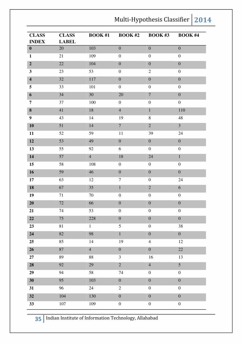
samples. The number of such classes is 64. We take 25 samples for each class. Out of these,
15 samples are for training, 5 samples are for testing and 5 samples are for validation. The
number of samples for each class from each book is shown:
Multi-Hypothesis Classifier 2014
35 Indian Institute of Information Technology, Allahabad
CLASS
INDEX
CLASS
LABEL
BOOK #1 BOOK #2 BOOK #3 BOOK #4
0 20 103 0 0 0
1 21 109 0 0 0
2 22 104 0 0 0
3 23 53 0 2 0
4 32 117 0 0 0
5 33 101 0 0 0
6 34 30 20 7 0
7 37 100 0 0 0
8 41 18 4 1 110
9 43 14 19 8 48
10 51 14 7 2 3
11 52 59 11 39 24
12 53 49 0 0 0
13 55 92 6 0 0
14 57 4 18 24 1
15 58 108 0 0 0
16 59 46 0 0 0
17 63 12 7 0 24
18 67 35 1 2 6
19 71 70 0 0 0
20 72 66 0 0 0
21 74 53 0 0 0
22 75 228 0 0 0
23 81 1 5 0 38
24 82 98 1 0 0
25 85 14 19 4 12
26 87 4 0 0 22
27 89 88 3 16 13
28 92 29 2 4 5
29 94 58 74 0 0
30 95 103 0 0 0
31 96 24 2 0 0
32 104 130 0 0 0
33 107 109 0 0 0

Multi-Hypothesis Classifier 2014
36 Indian Institute of Information Technology, Allahabad
34 111 77 18 0 0
35 115 0 0 0 94
36 135 210 0 0 0
37 141 43 14 2 0
38 142 43 7 11 0
39 143 23 102 0 0
40 145 83 0 0 0
41 148 86 0 0 0
42 152 51 0 0 0
43 156 16 4 0 14
44 158 40 1 0 0
45 159 77 0 0 0
46 166 105 0 0 0
47 170 78 8 5 27
48 171 109 0 0 3
49 172 36 2 1 0
50 175 68 175 0 4
51 176 83 0 0 0
52 178 26 1 3 2
53 180 21 0 1 3
54 181 90 4 0 5
55 201 34 13 59 18
56 202 103 0 0 0
57 217 65 30 0 0
58 219 70 1 7 6
59 220 19 0 6 123
60 221 0 0 0 117
61 222 232 2 0 0
62 224 89 36 9 13
63 231 0 0 245 0
Table 3.2: Distribution of data for classes with samples greater than 25.
Now, having seen the distribution of the data above, the next question arise is "how many
samples for each class from each book should be collected? " We have to ensure uniformity
in all respect. Equal number of samples should ideally be collected from each book. A logic

Multi-Hypothesis Classifier 2014
37 Indian Institute of Information Technology, Allahabad
is written which will determine the number of samples to be taken from each book for that
class, given the distribution of data. The algorithm is,
1) Check for the book with the minimum sample.
2) If ( Number of samples < 6) ; Take all the samples from that book.
3) Else ; Take only 6 samples from that book.
4) IF ( Last book? ), GOTO Step 6.
5) Go to the book with next minimum sample and repeat steps 2 &3.
6) Sum all the samples taken so far (sum) and take 25 - sum number of samples from the last
book.
Thus we have got a somewhat equally distributed samples from each book. Now, the next
dilemma is - "Which samples to collect from each class of each book, given the number of
samples to be collected from each book for each class?"
The best bet would be to use sampling theory, which would ensure good samples, which
represents the whole class distribution. But to keep things simple, a random function is used,
which will collect the required number of samples randomly from each book for each class.
After doing this the data distribution looks something like this:
CLASS
INDEX
CLASS
LABEL
BOOK #1 BOOK #2 BOOK #3 BOOK #4
0 20 25 0 0 0
1 21 25 0 0 0
2 22 25 0 0 0
3 23 23 0 2 0
4 32 25 0 0 0
5 33 25 0 0 0
6 34 13 6 6 0
7 37 25 0 0 0
8 41 6 4 1 14
9 43 6 6 6 7

Multi-Hypothesis Classifier 2014
38 Indian Institute of Information Technology, Allahabad
10 51 14 6 2 3
11 52 7 6 6 6
12 53 25 0 0 0
13 55 19 6 0 0
14 57 4 6 14 1
15 58 25 0 0 0
16 59 25 0 0 0
17 63 6 6 0 13
18 67 16 1 2 6
19 71 25 0 0 0
20 72 25 0 0 0
21 74 25 0 0 0
22 75 25 0 0 0
23 81 1 5 0 19
24 82 24 1 0 0
25 85 6 9 4 6
26 87 4 0 0 21
27 89 10 3 6 6
28 92 14 2 4 5
29 94 6 19 0 0
30 95 25 0 0 0
31 96 23 2 0 0
32 104 25 0 0 0
33 107 25 0 0 0
34 111 19 6 0 0
35 115 0 0 0 25
36 135 25 0 0 0
37 141 17 6 2 0
38 142 13 6 6 0
39 143 6 19 0 0
40 145 25 0 0 0
41 148 25 0 0 0
42 152 25 0 0 0

Multi-Hypothesis Classifier 2014
39 Indian Institute of Information Technology, Allahabad
43 156 15 4 0 6
44 158 24 1 0 0
45 159 25 0 0 0
46 166 25 0 0 0
47 170 8 6 5 6
48 171 22 0 0 3
49 172 22 2 1 0
50 175 6 15 0 4
51 176 25 0 0 0
52 178 19 1 3 2
53 180 21 0 1 3
54 181 16 4 0 5
55 201 6 6 7 6
56 202 25 0 0 0
57 217 19 6 0 0
58 219 12 1 6 6
59 220 6 0 6 13
60 221 0 0 0 25
61 222 23 2 0 0
62 224 7 6 6 6
63 231 0 0 25 0
Table 3.3: Distribution of samples selected from different books for each class.
Now let's take a look at the actual samples for each class. How do they actually look?
CLASS #20
CLASS INDEX #0
CLASS #21
CLASS INDEX #1
CLASS #22
CLASS INDEX #2
CLASS #23
CLASS INDEX #3
CLASS #32
CLASS INDEX #4
CLASS #33
CLASS INDEX #5
CLASS #34
CLASS INDEX #6
CLASS #37
CLASS INDEX #7

Multi-Hypothesis Classifier 2014
40 Indian Institute of Information Technology, Allahabad
CLASS #41
CLASS INDEX #8
CLASS #43
CLASS INDEX #9
CLASS #51
CLASS INDEX #10
CLASS #52
CLASS INDEX #11
CLASS #53
CLASS INDEX #12
CLASS #55
CLASS INDEX #13
CLASS #57
CLASS INDEX #14
CLASS #58
CLASS INDEX #15
CLASS #59
CLASS INDEX #16
CLASS #63
CLASS INDEX #17
CLASS #67
CLASS INDEX #18
CLASS #71
CLASS INDEX #19
CLASS #72
CLASS INDEX #20
CLASS #74
CLASS INDEX #21
CLASS #75
CLASS INDEX #22
CLASS #81
CLASS INDEX #23
CLASS #82
CLASS INDEX #24
CLASS #85
CLASS INDEX #25
CLASS #87
CLASS INDEX #26
CLASS #89
CLASS INDEX #27
CLASS #92
CLASS INDEX #28
CLASS #94
CLASS INDEX #29
CLASS #95
CLASS INDEX #30
CLASS #96
CLASS INDEX #31
CLASS #104
CLASS INDEX #32
CLASS #107
CLASS INDEX #33
CLASS #111
CLASS INDEX #34
CLASS #115
CLASS INDEX #35
CLASS #135
CLASS INDEX #36
CLASS #141
CLASS INDEX #37
CLASS #142
CLASS INDEX #38
CLASS #143
CLASS INDEX #39
CLASS #145
CLASS INDEX #40
CLASS #148
CLASS INDEX #41
CLASS #152
CLASS INDEX #42
CLASS #156
CLASS INDEX #43

Multi-Hypothesis Classifier 2014
41 Indian Institute of Information Technology, Allahabad
CLASS #158
CLASS INDEX #44
CLASS #159
CLASS INDEX #45
CLASS #166
CLASS INDEX #46
CLASS #170
CLASS INDEX #47
CLASS #171
CLASS INDEX #48
CLASS #172
CLASS INDEX #49
CLASS #175
CLASS INDEX #50
CLASS #176
CLASS INDEX #51
CLASS #178
CLASS INDEX #52
CLASS #180
CLASS INDEX #53
CLASS #181
CLASS INDEX #54
CLASS #201
CLASS INDEX #55
CLASS #202
CLASS INDEX #56
CLASS #217
CLASS INDEX #57
CLASS #219
CLASS INDEX #58
CLASS #220
CLASS INDEX #59
CLASS #221
CLASS INDEX #60
CLASS #222
CLASS INDEX #61
CLASS #224
CLASS INDEX #62
CLASS #231
CLASS INDEX #63
Table 3.4: Visual appearance of the dataset
Now, having known the dataset, we move forward to the formation of the individual
classifiers. Also one more important factor to be noted, due to the different sizes of the
images collected, all the images are first resized to a fixed dimension of 32x32. And to
remove any unwanted grey values in the images, a threshold is applied to completely binarize
the images.
3.2 Software and source code used
The language used to code is C++.
Library used is OPEN-CV.
Classifier-1: Classifier-1 is formed by simply using a nearest neighbour approach on the raw
pixel values. The images are read, and stored as column vectors in three matrices, namely
training, testing and validation. The metrics used for measurement is Euclidean distance. This

Multi-Hypothesis Classifier 2014
42 Indian Institute of Information Technology, Allahabad
is the cheapest algorithm used among the three. The result of this classifier is represented in
the form of a confusion matrix.
Classifier-2: Classifier-2 is a tricky one. In this classifier, instead of directly using the raw
pixels as feature vector, we extract feature explicitly from the images. Next query would be
what is the feature vector? To extract the feature from a given image, we first have to find the
centroid of the image. Centroid can be found using a weighted mean approach in both
horizontal and vertical direction and arriving at a particular value of x and y which becomes
the centroid. Now, from the centroid, a vector is drawn up to the edge of the image vertically,
and rotated a full 360 degrees. While doing so, the distance between the centroids and the last
black pixel encountered on that vector, while moving from the centroids towards the edge of
the image is noted down. This distance is noted down for all the vectors in the entire span of
the image. Thus from an image, we obtain a feature vector of all the distances from the
centroids to the edge points.
Fig 3.1: Calculating the distance of the last black pixel along the vector drawn from the
centroids to the perimeter of the image.
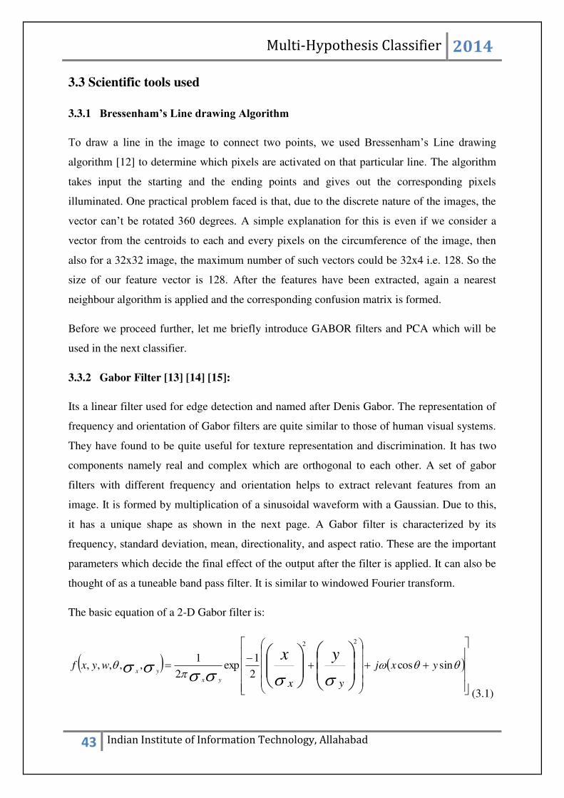
Multi-Hypothesis Classifier 2014
43 Indian Institute of Information Technology, Allahabad
3.3 Scientific tools used
3.3.1 Bressenham’s Line drawing Algorithm
To draw a line in the image to connect two points, we used Bressenham’s Line drawing
algorithm [12] to determine which pixels are activated on that particular line. The algorithm
takes input the starting and the ending points and gives out the corresponding pixels
illuminated. One practical problem faced is that, due to the discrete nature of the images, the
vector can’t be rotated 360 degrees. A simple explanation for this is even if we consider a
vector from the centroids to each and every pixels on the circumference of the image, then
also for a 32x32 image, the maximum number of such vectors could be 32x4 i.e. 128. So the
size of our feature vector is 128. After the features have been extracted, again a nearest
neighbour algorithm is applied and the corresponding confusion matrix is formed.
Before we proceed further, let me briefly introduce GABOR filters and PCA which will be
used in the next classifier.
3.3.2 Gabor Filter [13] [14] [15]:
Its a linear filter used for edge detection and named after Denis Gabor. The representation of
frequency and orientation of Gabor filters are quite similar to those of human visual systems.
They have found to be quite useful for texture representation and discrimination. It has two
components namely real and complex which are orthogonal to each other. A set of gabor
filters with different frequency and orientation helps to extract relevant features from an
image. It is formed by multiplication of a sinusoidal waveform with a Gaussian. Due to this,
it has a unique shape as shown in the next page. A Gabor filter is characterized by its
frequency, standard deviation, mean, directionality, and aspect ratio. These are the important
parameters which decide the final effect of the output after the filter is applied. It can also be
thought of as a tuneable band pass filter. It is similar to windowed Fourier transform.
The basic equation of a 2-D Gabor filter is:
sincos2
1exp
2
1,,,,,
22
yxj
yx
wyxfyx
yx
yx
(3.1)

Multi-Hypothesis Classifier 2014
44 Indian Institute of Information Technology, Allahabad
Where,
x= Standard deviation along x-axis
y= Standard deviation along y-axis.
Θ = Orientation or the angle
ω = Frequency
Figure 3.2: A visual representation of a 2-D Gabor filter
This is especially important for OCR applications due to its unique shape and flexibility. It
gives varied response (weak/strong) depending on the orientation and frequency of the filter
which makes it ideal for stroke detection applications. A typical example of the effect of a
Gabor bank with different orientation on a Chinese character is shown below:

Multi-Hypothesis Classifier 2014
45 Indian Institute of Information Technology, Allahabad
Figure 3.3: Gabor Filter bank with four different orientations (0, 45, 90, 135) are shown
on the right. The original is shown in the top left and below it is the superposition of all
the Gabor images.
Now after having a brief idea about GABOR filters, let’s introduce our next topic, PCA
(Principal component analysis).
3.3.3 Principal Component Analysis [16]
PCA is a dimension reduction technique and is used extensively in modern day to day
applications. Due to the large size of our feature vectors and also due to the redundancy of
information, PCA comes as a rescue to help distinguish relevant features which conveys
relevant information from the irrelevant ones. The basic principle on which PCA works is
that it tries to fit in a lower dimension hyper-plane, on which the projections of the data
points would have maximum variance. In simple words, it tries to minimize the projection
error. It sounds quite similar to regression, although there is a very simple difference between
the two,

Multi-Hypothesis Classifier 2014
46 Indian Institute of Information Technology, Allahabad
Figure 3.4: Regression (left) v/s PCA (right).
The Figure in the left shows regression whose objective is to minimise the output error. On
the other hand PCA minimises the projection error. The basic steps to implement PCA are as
follows:
1) Get some data
2) Subtract the mean
3) Calculate the Covariance matrix
4) Calculate the Eigen values and corresponding Eigen vectors of the covariance matrix.
5) Choosing the required number of components and forming the feature vector.
The last step is the deciding step in maintaining the required variance of the data. After
computing the Eigen values of the covariance matrix, it is found that only few Eigen values
are significant compared to the rest. It signifies that the data is distributed along that Eigen
vector more whose values are higher. This will help to discriminate between different classes
even if we discard the Eigen vectors where there is no visible variance, which leads to
dimension reduction. Now we have the required tools ready to discuss the Classifier-3.
Classifier-3: This is the most decorated and expensive classifier used among the three. This
classifier again extracts some features from the images. Feature extracted are by the means of
a GABOR filter bank. The important point to be noted is how the Gabor filter has been used
on the image? A GABOR kernel of size 5x5 is selected and convoluted on the whole image
(size 32x32) starting from the top left each one with four different orientations (0, 45, 90,
Multi-Hypothesis Classifier 2014
47 Indian Institute of Information Technology, Allahabad
135) which will generate a feature vector of size 4096. After this, we apply PCA to reduce
the dimension from 4096 to 100 (optimum). After the feature vectors are formed, this is fed
to our plain old nearest neighbour algorithm and the corresponding confusion matrix is
created.
Now having done with the formation of the classifiers, we now proceed to the formation of
the hypotheses. Five different hypotheses are formed. The description of each one of them is
given below:
3.4 HYPOTHESIS #1
The confusion matrix is formed for each classifier. The confusion matrix is a square matrix
(no. of rows = no. of class labels) which gives a general idea of which samples are classified
in to which class. Using the confusion matrix, we create the confidence matrix which shows
the confidence of each classifier for a given class label. Confidence matrix is created by
taking the ratio of the diagonal element and the sum of that particular column and doing this
for all the class labels. After this is done, next when a validation data is entered, all the
classifiers predict its class label for that particular sample. Now we can use the confidence
matrix as a lookup table and compare the confidence of the given classifiers on the predicted
class labels. In case two or more classifiers predict the same class label then the confidence
for that predicted class adds up. Finally to take a final decision, the hypothesis checks which
class label has got the highest confidence value and that class label is selected as the final
predicted class label of the hypothesis.
3.5 HYPOTHESIS #2
The basic strategy of this hypothesis is to exploit the distance between the best match and the
second best match. More the distance of the best match and second best, more is the
probability of that sample belonging to that particular class (best match). To explain in more
detail, for a given test sample, the best match is found from the same class label from the
training set and denoted as dis1. Then the same sample is found the second best match from
the remaining training set (apart from the samples already scanned) and denoted as dis2. Now

Multi-Hypothesis Classifier 2014
48 Indian Institute of Information Technology, Allahabad
the ratio dis2/dis1 gives a general idea about how far is the second best from the best match.
More the ratio more the confidence. Now for every validation data that enters, we already
have a set of built confidence values for each test sample from each classifier. Now, we just
apply nearest neighbour on the validation set and form a result matrix which shows which
classifiers predicted which class labels. After this, just compare the confidence obtained
earlier for that sample number, and the classifier with the maximum confidence will have its
final say in the voting.
3.6 HYPOTHESIS #3
This hypothesis takes in to account the centroids of each class labels. Each sample is
compared to the class centroids, and the nearest match is noted. If the class label index
matches with the test sample index, then we have a correct classification otherwise not. Using
this information the confusion matrix is created for each classifier. Using the confusion
matrix, confidence matrix is formed. Now, when a validation data comes, it is passed through
the same procedure as the test data set has gone through. The classifiers will output a certain
class label as its output. Now, the confidence matrix comes handy to decide which classifier
has a higher confidence for that particular class label. Using weighted majority voting, the
final decision of the hypothesis is decided.
3.7 HYPOTHESIS #4
This hypothesis takes off from the previous hypothesis. In this method, along with the
centroids, the average distances of the samples from their respective centroids are calculated.
The test samples are compared with the centroids and the minimum distance of that sample
from all the centroids are found out. Now this distance is compared with all the "average
distances for each class" that was previously calculated and the nearest match is found and
the index is noted. This metric is used to form the confusion matrix. From the confusion
matrix, confidence matrix is again created. Now for the validation data, the same procedure is
repeated and the index is noted for the nearest match, which becomes the predicted class for
that particular classifier. Now to arrive at a final decision, the confidence matrix is referred

Multi-Hypothesis Classifier 2014
49 Indian Institute of Information Technology, Allahabad
and based on the confidence of each classifier on particular predicted class labels, the final
decision is made.
3.8 HYPOTHESIS #5
This hypothesis avoids the confusion matrix and directly calculates the confidence matrix
using the ratio of average class distances and the nearest match from the centroids. If the
nearest match is smaller, then the ratio will be higher indicating strong confidence of the
classifier for that class label. Ideally the confidence of each classifier for each class should be
close to 1.
The result and the analysis for each of the above hypotheses will be discussed in the next
section.

Multi-Hypothesis Classifier 2014
50 Indian Institute of Information Technology, Allahabad
Chapter 4
Results and Analysis
4.1 Hypothesis #1
4.1.1 Analysis of Classifier #1
Figure 4.1: Confusion matrix of classifier-1(Nearest neighbour algorithm)
Conclusion: Accuracy obtained is 84.06 %.

Multi-Hypothesis Classifier 2014
51 Indian Institute of Information Technology, Allahabad
4.1.2 Analysis of Classifier #2
Figure 4.2: Confusion matrix of classifier-2 (Centroid feature extraction method)
Conclusion: Accuracy obtained is 79.06%.

Multi-Hypothesis Classifier 2014
52 Indian Institute of Information Technology, Allahabad
4.1.3 Analysis of the PCA on accuracy of the Classifier #3
Before proceeding to the next classifier results (GABOR+PCA+Nearest neighbour), the
analysis for the optimum GABOR filter and PCA combination is shown. The below table
shows the comparison between the number of principal components retained and its effect on
the overall accuracy of the classifier.
Number of Principal components
retained
Final accuracy of the classifier
20 60.62 %
30 63.75 %
40 68.75 %
50 69.37 %
60 70.62 %
70 71.56 %
80 71.56 %
90 72.81 %
100 73.12 %
110 74.37 %
120 74.37 %
130 74.06 %
140 74.06 %
Table 4.1: Number of components retained v/s classifier accuracy.
Conclusion: From the above table, it is concluded that retaining 110 principal components
gives the maximum accuracy. Also the accuracy decreases if the number of principal
components is more than 120.

Multi-Hypothesis Classifier 2014
53 Indian Institute of Information Technology, Allahabad
4.1.4 Effect of the size of GABOR kernel on the accuracy of Classifier #3
The effect of the size of the GABOR kernel on the accuracy of the classifier is shown below.
The below is calculated keeping the number of principal components at 110.
Size of the GABOR kernel Accuracy
3 64.68 %
4 70.62 %
5 70.62 %
6 74.06 %
7 74.37 %
8 73.75 %
9 73.75 %
10 71.56 %
Table 4.2: Size of Gabor kernel v/s classifier accuracy
Conclusion: From the above table we conclude that accuracy increases as the size of the
kernel increases up to a certain point and then it starts to decrease. For the size of kernel
being at 7, the maximum accuracy of the classifier is achieved at 74.37 %.

Multi-Hypothesis Classifier 2014
54 Indian Institute of Information Technology, Allahabad
4.1.5 Analysis of classifier-3 (GABOR + PCA + Nearest Neighbour)
Fig 4.3: Confusion matrix of classifier #3
Conclusion: The accuracy obtained is 74.37 %.

Multi-Hypothesis Classifier 2014
55 Indian Institute of Information Technology, Allahabad
4.1.6 Confidence Matrix
Figure 4.4: Confidence matrix of the 3 classifiers

Multi-Hypothesis Classifier 2014
56 Indian Institute of Information Technology, Allahabad
4.1.7 Summary of Hypothesis #1

Multi-Hypothesis Classifier 2014
57 Indian Institute of Information Technology, Allahabad

Multi-Hypothesis Classifier 2014
58 Indian Institute of Information Technology, Allahabad
Figure 4.5: Summary of the final hypothesis.

Multi-Hypothesis Classifier 2014
59 Indian Institute of Information Technology, Allahabad
4.1.8 Conclusion from Hypothesis #1
From the above result we infer that Class label #43 is always getting classified as Class label
#60 and Class label #59 is getting classified as Class label #35, due to visual similarity
between the two class samples. Some examples pair of data with visual similarity which our
classifiers are not able to classify properly are given below:
CLASS #156
CLASS INDEX #43
CLASS #221
CLASS INDEX #60
CLASS #224
CLASS INDEX #62
CLASS #178
CLASS INDEX #52
CLASS #145
CLASS INDEX #40
CLASS #221
CLASS INDEX #60
Some examples of bad classes on which all the classifiers fail most of the time:
CLASS #141
CLASS INDEX #37 CLASS #89
CLASS INDEX #27
CLASS #67
CLASS INDEX #18
CLASS #217
CLASS INDEX #57
CLASS #219
CLASS INDEX #58
CLASS #170
CLASS INDEX #47

Multi-Hypothesis Classifier 2014
60 Indian Institute of Information Technology, Allahabad
Now, for our hypothesis to work decently at least one classifier should give the correct
prediction. The number of such samples from the above observation is 255. Among them, the
number of correctly classified samples by the hypothesis is 223. So our final accuracy stands
at 87.45 %.
ACCURACY = 87.45 %
The samples discarded are: 44, 54, 59, 65, 66, 67, 68, 69, 74, 76, 87, 90, 91, 92, 93, 94, 136,
158, 159, 170, 171, 172, 185, 186, 187, 193, 195, 204, 215, 216, 217, 218, 219, 224, 235,
239, 243, 247, 248, 249, 257, 263, 264, 267, 271, 273, 274, 285, 287, 288, 289, 290, 293,
294, 295, 296, 297, 298, 299, 308, 309, 310, 311, 313, 314.

Multi-Hypothesis Classifier 2014
61 Indian Institute of Information Technology, Allahabad
4.2 HYPOTHESIS #2
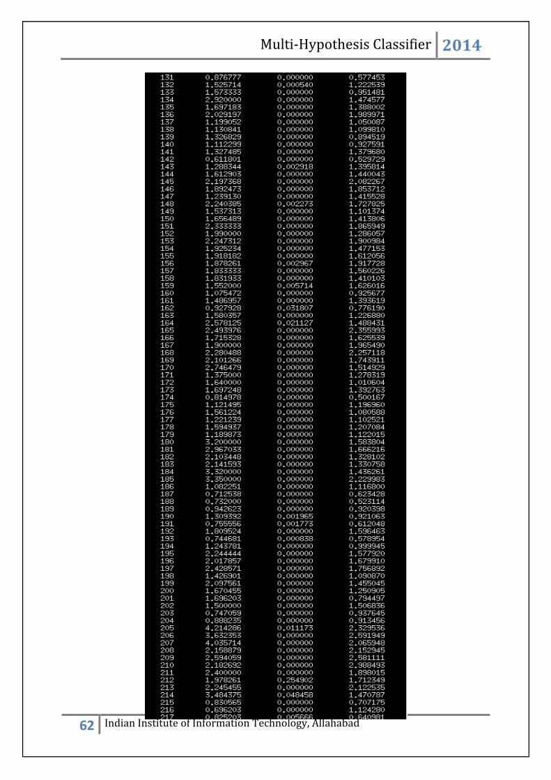
Multi-Hypothesis Classifier 2014
62 Indian Institute of Information Technology, Allahabad
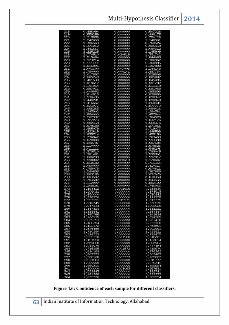
Multi-Hypothesis Classifier 2014
63 Indian Institute of Information Technology, Allahabad
Figure 4.6: Confidence of each sample for different classifiers.
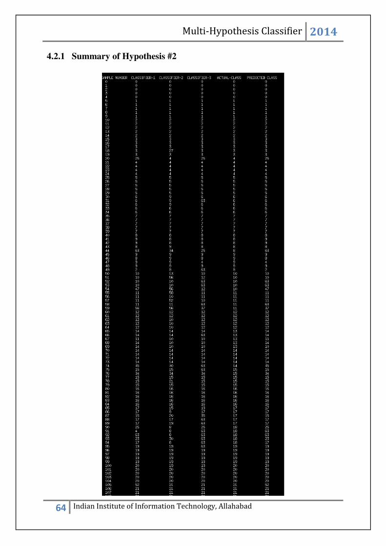
Multi-Hypothesis Classifier 2014
64 Indian Institute of Information Technology, Allahabad
4.2.1 Summary of Hypothesis #2

Multi-Hypothesis Classifier 2014
65 Indian Institute of Information Technology, Allahabad
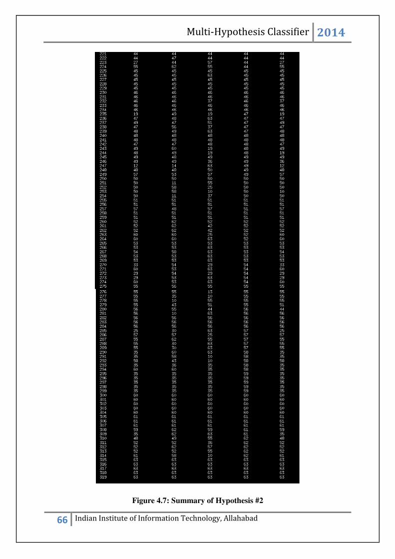
Multi-Hypothesis Classifier 2014
66 Indian Institute of Information Technology, Allahabad
Figure 4.7: Summary of Hypothesis #2

Multi-Hypothesis Classifier 2014
67 Indian Institute of Information Technology, Allahabad
4.2.2 CONCLUSION FROM HYPOTHESIS #2
The first conclusion that can be drawn from Hypothesis #2 is that the confidence of the
classifier-2 is zero in most of the cases, which suggests that this classifier will have lesser
impact on the voting of the confidences during the formation of the hypothesis.
A very interesting observation is that from sample number 45 to 49 which belongs to class
index #9 out of all the three classifiers, only classifier #2 is predicting this class correctly, but
due to zero confidence of classifier #2 on those samples, the correct classification is bypassed
and wrong prediction is obtained by the hypothesis. This shows that the technique used for
the formation of the confidence matrix may not be reliable at all time.
In this method of hypothesis formation some observations are as follows:
Class index #13 and #43 is always getting miss-classified as class index #14 and #60
respectively.
CLASS #55
CLASS INDEX #13
CLASS #57
CLASS INDEX #14
CLASS #156
CLASS INDEX #43
CLASS #221
CLASS INDEX #60
CLASS #220
CLASS INDEX #59
CLASS #115
CLASS INDEX #35
Apart from these classes which exhibit unusual similarity, there are some other classes for
which the hypothesis is not able to correctly predict the output and making random errors.

Multi-Hypothesis Classifier 2014
68 Indian Institute of Information Technology, Allahabad
Those class indices are #18(5/5 misclassification), #54(5/5 misclassification), #57(4/5
misclassification), #58(4/5 misclassification), #62 (5/5 misclassification).
CLASS #67
CLASS INDEX #18
CLASS #181
CLASS INDEX #54
CLASS #217
CLASS INDEX #57
CLASS #219
CLASS INDEX #58 CLASS #224
CLASS INDEX #62
Also the best class in which every single classifier is giving the correct prediction which
leads to correct overall prediction is class index #42.
CLASS #152
CLASS INDEX #42
Again, for this hypothesis to work decently, only those samples are considered which is
correctly being classified by at least one of the classifiers. The number of such samples are
255. And the number of correctly predicted samples by the hypothesis is 226. So the accuracy
comes to 88.62 %.
ACCURACY = 88.62 %
The samples discarded are: 44, 54, 59, 65, 66, 67, 68, 69, 74, 76, 87, 90, 91, 92, 93, 94, 136,
158, 159, 170, 171, 172, 185, 186, 187, 193, 195, 204, 215, 216, 217, 218, 219, 224, 235,
239, 243, 247, 248, 249, 257, 263, 264, 267, 271, 273, 274, 285, 287, 288, 289, 290, 293,
294, 295, 296, 297, 298, 299, 308, 309, 310, 311, 313, 314.
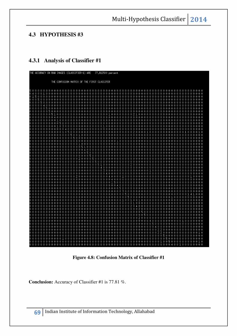
Multi-Hypothesis Classifier 2014
69 Indian Institute of Information Technology, Allahabad
4.3 HYPOTHESIS #3
4.3.1 Analysis of Classifier #1
Figure 4.8: Confusion Matrix of Classifier #1
Conclusion: Accuracy of Classifier #1 is 77.81 %.
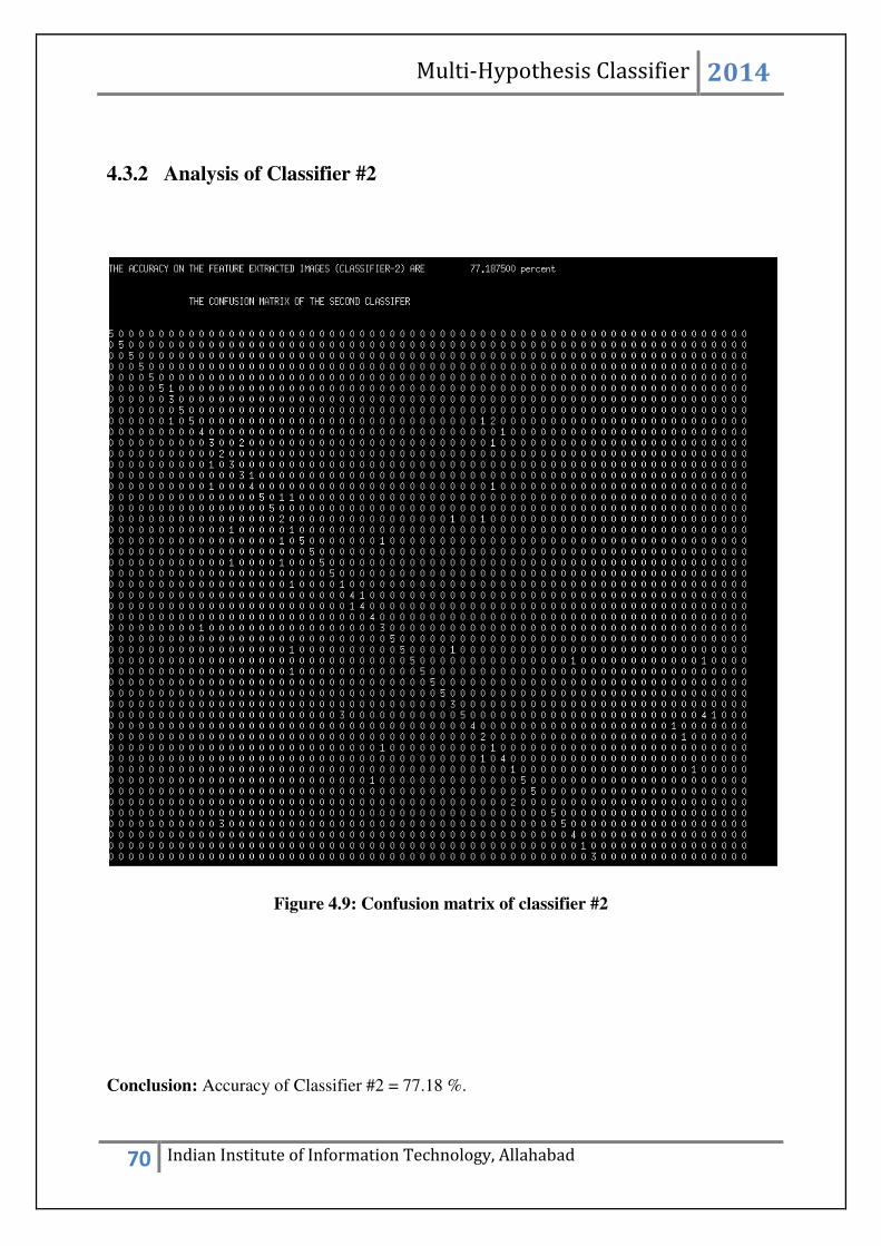
Multi-Hypothesis Classifier 2014
70 Indian Institute of Information Technology, Allahabad
4.3.2 Analysis of Classifier #2
Figure 4.9: Confusion matrix of classifier #2
Conclusion: Accuracy of Classifier #2 = 77.18 %.

Multi-Hypothesis Classifier 2014
71 Indian Institute of Information Technology, Allahabad
4.3.3 Analysis of Classifier #3
Fig 4.10: Confusion matrix of classifier #3
Conclusion: Accuracy of Classifier #3 = 60.62 %.

Multi-Hypothesis Classifier 2014
72 Indian Institute of Information Technology, Allahabad
4.3.4 Confidence Matrix
Fig 4.11: Confidence matrix of hypothesis #3.

Multi-Hypothesis Classifier 2014
73 Indian Institute of Information Technology, Allahabad
4.3.5 Summary of Hypothesis #3
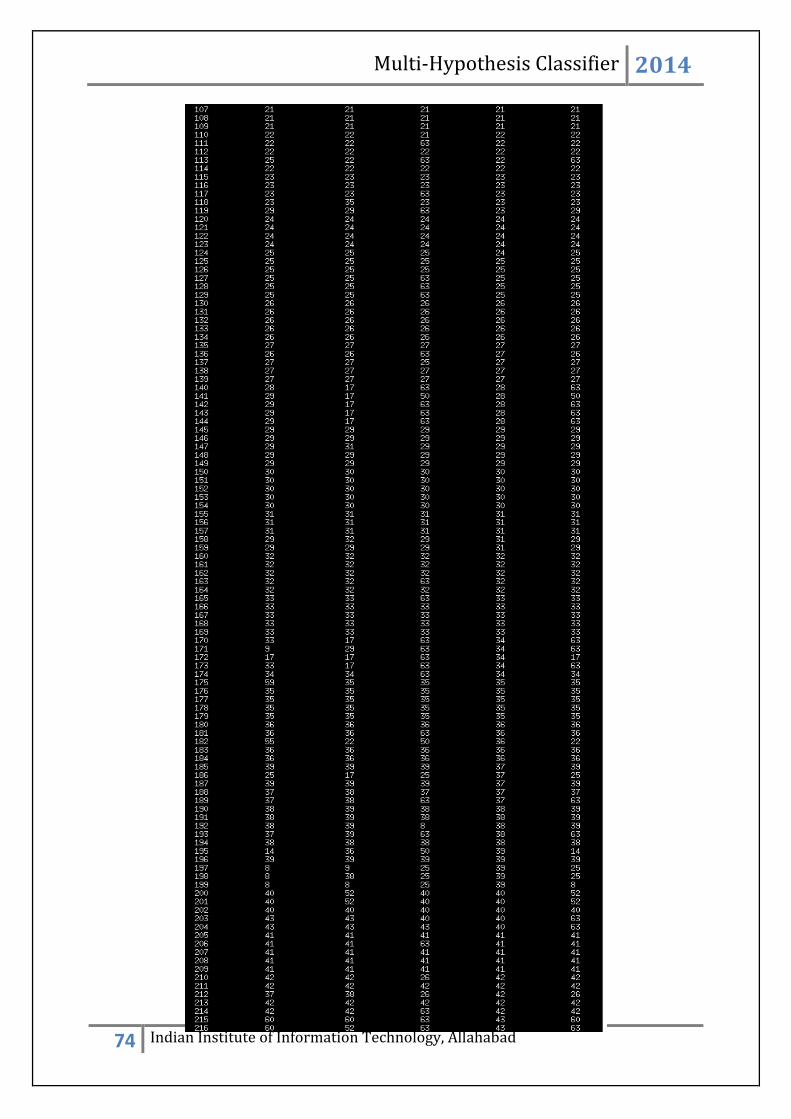
Multi-Hypothesis Classifier 2014
74 Indian Institute of Information Technology, Allahabad

Multi-Hypothesis Classifier 2014
75 Indian Institute of Information Technology, Allahabad
Fig 4.12: Summary of Hypothesis #3
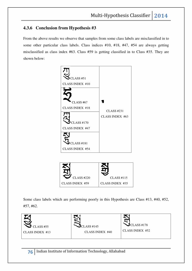
Multi-Hypothesis Classifier 2014
76 Indian Institute of Information Technology, Allahabad
4.3.6 Conclusion from Hypothesis #3
From the above results we observe that samples from some class labels are misclassified in to
some other particular class labels. Class indices #10, #18, #47, #54 are always getting
misclassified as class index #63. Class #59 is getting classified in to Class #35. They are
shown below:
CLASS #51
CLASS INDEX #10
CLASS #231
CLASS INDEX #63
CLASS #67
CLASS INDEX #18
CLASS #170
CLASS INDEX #47
CLASS #181
CLASS INDEX #54
CLASS #220
CLASS INDEX #59
CLASS #115
CLASS INDEX #35
Some class labels which are performing poorly in this Hypothesis are Class #13, #40, #52,
#57, #62.
CLASS #55
CLASS INDEX #13
CLASS #145
CLASS INDEX #40
CLASS #178
CLASS INDEX #52

Multi-Hypothesis Classifier 2014
77 Indian Institute of Information Technology, Allahabad
CLASS #217
CLASS INDEX #57 CLASS #224
CLASS INDEX #62
For the hypothesis to work correctly, those samples are considered on which at least one
classifier has given a correct prediction. Using the above table, we find that there are 233
such samples, out of which the number of correctly classified samples by the hypothesis are
194. Thus the final accuracy is 83.26%.
ACCURACY = 83.26 %
The samples discarded are: 18, 44, 50, 51, 52, 53, 54, 58, 59, 65, 66, 67, 68, 69, 74, 76, 87,
119, 124, 136, 141, 142, 143, 144, 158, 159, 170, 171, 172, 173, 182, 185, 186, 187, 192,
193, 195, 197, 199, 204, 215, 216, 217, 218, 219, 223, 224, 235, 236, 237, 238, 239, 244,
246, 247, 248, 249, 251, 254, 257, 261, 262, 263, 264, 267, 271, 274, 279, 285, 286, 287,
288, 289, 290, 293, 294, 296, 297, 298, 299, 308, 309, 310, 311, 312, 313, 314.
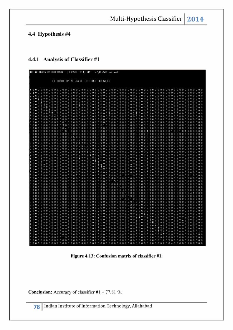
Multi-Hypothesis Classifier 2014
78 Indian Institute of Information Technology, Allahabad
4.4 Hypothesis #4
4.4.1 Analysis of Classifier #1
Figure 4.13: Confusion matrix of classifier #1.
Conclusion: Accuracy of classifier #1 = 77.81 %.

Multi-Hypothesis Classifier 2014
79 Indian Institute of Information Technology, Allahabad
4.4.2 Analysis of classifier #2
Figure 4.14: Confusion matrix of classifier #2.
Conclusion: Accuracy of classifier #2 = 63.12 %.

Multi-Hypothesis Classifier 2014
80 Indian Institute of Information Technology, Allahabad
4.4.3 Analysis of classifier #3
Fig 4.15: Confusion matrix of classifier #3
Conclusion: Accuracy of classifier #3 = 4.37 %. Most of the samples are getting incorrectly
classified.

Multi-Hypothesis Classifier 2014
81 Indian Institute of Information Technology, Allahabad
4.4.4 Confidence matrix
Figure 4.16: Confidence matrix of Hypothesis #4
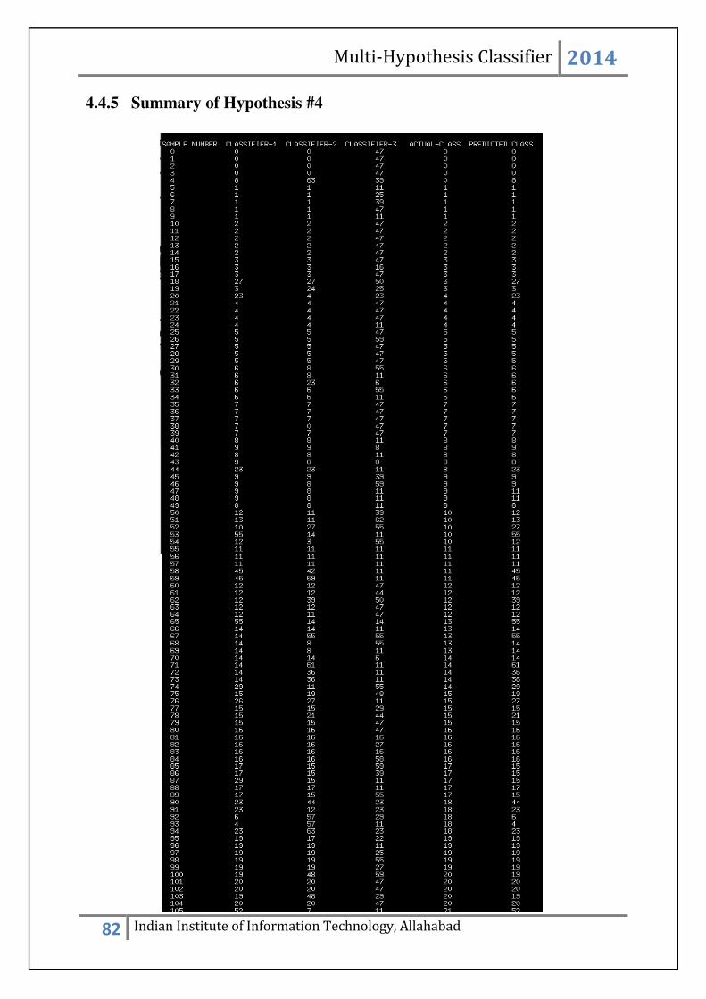
Multi-Hypothesis Classifier 2014
82 Indian Institute of Information Technology, Allahabad
4.4.5 Summary of Hypothesis #4

Multi-Hypothesis Classifier 2014
83 Indian Institute of Information Technology, Allahabad
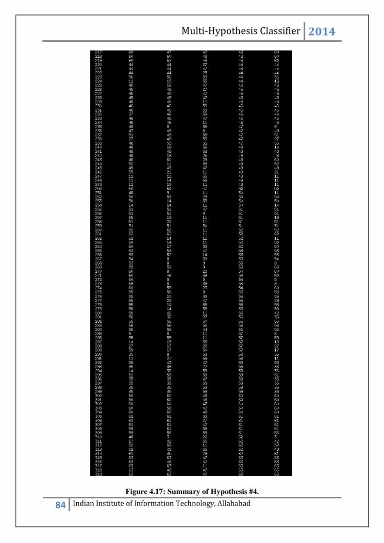
Multi-Hypothesis Classifier 2014
84 Indian Institute of Information Technology, Allahabad
Figure 4.17: Summary of Hypothesis #4.

Multi-Hypothesis Classifier 2014
85 Indian Institute of Information Technology, Allahabad
4.4.6 Conclusion from Hypothesis #4
Samples from class #28 are getting misclassified as class #29 (4/5 times). Similarly, class
#43, #54, #59 is getting misclassified in to class #60, #60, #35 (4/5 times). The visual
comparison is shown below:
CLASS #92
CLASS INDEX #28
CLASS #94
CLASS INDEX #29
CLASS #156
CLASS INDEX #43
CLASS #221
CLASS INDEX #60
CLASS #181
CLASS INDEX #54
CLASS #221
CLASS INDEX #60
CLASS #220
CLASS INDEX #59
CLASS #115
CLASS INDEX #35
The class indices #10, #13, #14, #18, #28, #54, #62 cannot be correctly classified by the
hypothesis as most of the samples are being misclassified by the individual classifiers as well.
CLASS #51
CLASS INDEX #10
CLASS #55
CLASS INDEX #13 CLASS #57
CLASS INDEX #14
CLASS #67
CLASS INDEX #18

Multi-Hypothesis Classifier 2014
86 Indian Institute of Information Technology, Allahabad
CLASS #92
CLASS INDEX #28
CLASS #181
CLASS INDEX #54
CLASS #224
CLASS INDEX #62
Again, for this hypothesis to work, those samples will be considered which has been correctly
classified by at least one of the three classifiers. Number of such samples are 227. Also the
number of correctly classified samples by the hypothesis is 190. So the accuracy amounts to
83.7 %.
ACCURACY = 83.7 %
The samples discarded are: 4, 18, 44, 49, 50, 51, 53, 54, 65, 66, 67, 68, 69, 74, 76, 87, 90, 91,
92, 93, 94, 100, 103, 105, 113, 124, 136, 158, 159, 170, 172, 173, 175, 182, 185, 186, 187,
192, 193, 195, 203, 204, 212, 215, 216, 217, 218, 219, 223, 224, 235, 237, 238, 239, 244,
246, 247, 248, 249, 251, 254, 257, 261, 262, 263, 264, 267, 269, 270, 271, 272, 273, 274,
285, 286, 287, 288, 289, 290, 291, 293, 294, 295, 296, 297, 298, 299, 309, 310, 311, 312,
313, 314.

Multi-Hypothesis Classifier 2014
87 Indian Institute of Information Technology, Allahabad
4.5 Hypothesis #5

Multi-Hypothesis Classifier 2014
88 Indian Institute of Information Technology, Allahabad

Multi-Hypothesis Classifier 2014
89 Indian Institute of Information Technology, Allahabad
Figure 4.18: Summary of Hypothesis #5

Multi-Hypothesis Classifier 2014
90 Indian Institute of Information Technology, Allahabad
4.5.1 Conclusions from Hypothesis #5
The above table shows the predicted class labels from each classifiers along with the
confidence values of each classifier on that sample which leads to the final decision making.
From the above table we can observe that class index #54 and #57 are difficult to classify
correctly as each one of the single classifier fails to classify them. Also class index #59 and
#43 are getting misclassified to class index #35 and #60 every single time, just like in the
previous cases. A new observation reveals that class index #13 and #14 are indistinguishable,
i.e. every time class #13 predicts #14 as its output.
CLASS #181
CLASS INDEX #54
CLASS #217
CLASS INDEX #57
CLASS #55
CLASS INDEX #13
CLASS #57
CLASS INDEX #14
CLASS #220
CLASS INDEX #59
CLASS #115
CLASS INDEX #35
For this hypothesis to work decently, those samples are considered on which at least one
classifier has predicted the correct class index. The number of such samples is 228. Also the
number of correctly classified samples is 191. Thus the accuracy stands at 83.77 %.
ACCURACY = 83.77 %

Multi-Hypothesis Classifier 2014
91 Indian Institute of Information Technology, Allahabad
The discarded samples are: 4, 18, 44, 49, 50, 51, 53, 54, 65, 66, 67, 68, 69, 74, 76, 87, 90, 91,
92, 93 ,94, 100, 103, 105, 113, 124, 136, 158, 159, 170, 172, 173, 175, 182, 185, 186, 187,
192, 193, 195, 203, 204, 212, 215, 216, 217, 218, 219, 223, 224, 235, 237, 238, 239, 244,
246, 247, 248, 249, 251, 254, 257, 261, 262, 263, 264, 267, 269, 270, 271, 272, 273, 274,
285, 286, 287, 288, 289, 290, 291, 293, 294, 296, 297, 298, 299, 309, 310, 311, 312, 313,
314.
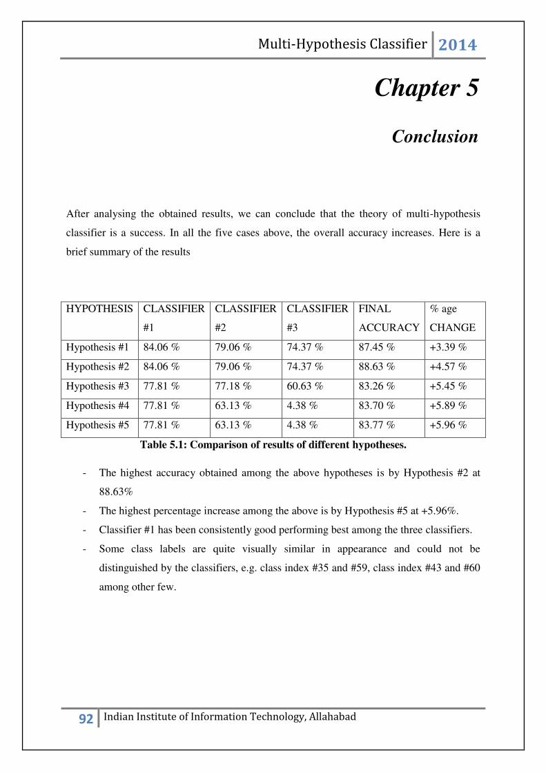
Multi-Hypothesis Classifier 2014
92 Indian Institute of Information Technology, Allahabad
Chapter 5
Conclusion
After analysing the obtained results, we can conclude that the theory of multi-hypothesis
classifier is a success. In all the five cases above, the overall accuracy increases. Here is a
brief summary of the results
HYPOTHESIS CLASSIFIER
#1
CLASSIFIER
#2
CLASSIFIER
#3
FINAL
ACCURACY
% age
CHANGE
Hypothesis #1 84.06 % 79.06 % 74.37 % 87.45 % +3.39 %
Hypothesis #2 84.06 % 79.06 % 74.37 % 88.63 % +4.57 %
Hypothesis #3 77.81 % 77.18 % 60.63 % 83.26 % +5.45 %
Hypothesis #4 77.81 % 63.13 % 4.38 % 83.70 % +5.89 %
Hypothesis #5 77.81 % 63.13 % 4.38 % 83.77 % +5.96 %
Table 5.1: Comparison of results of different hypotheses.
- The highest accuracy obtained among the above hypotheses is by Hypothesis #2 at
88.63%
- The highest percentage increase among the above is by Hypothesis #5 at +5.96%.
- Classifier #1 has been consistently good performing best among the three classifiers.
- Some class labels are quite visually similar in appearance and could not be
distinguished by the classifiers, e.g. class index #35 and #59, class index #43 and #60
among other few.
Multi-Hypothesis Classifier 2014
93 Indian Institute of Information Technology, Allahabad
Chapter 6
Future Scope
Active research has been going on and there is still lot to be done in this field. Some future
enhancements are suggested below:
1) Increase number of Classifiers: Some more number of classifiers can be used such
as SVM, ANN, Fringe maps and the overall effect of using theses can be analysed.
2) Sampling techniques: One particular observation drawn from this research is the
conflicts of results given on the test set and the validation set by a particular classifier
for their respective sample numbers, i.e. for samples belonging to a particular class
label, the prediction by a particular classifier on the data of test and validation set
conflicts, which resulted in some samples being discarded and also affected in the
overall accuracy. We have used a random sample selector to select our data randomly.
A better way could be to use sampling techniques. Sampling techniques ensure that
the selected samples are well represented by that class. As data plays a huge role in
deciding the accuracy, intelligent way of sampling the data could be a major boost to
improve the accuracy.
3) Forming the perfect ensemble: The basic assumption made on this research is that
the classifiers are mutually exclusive i.e. statistically independent. Although we
haven’t exactly explored how to achieve this or how to prove if they are mutually
complementary. Work can be pursued in this direction to form the perfect ensemble,
which will have a direct impact on the accuracy.

Multi-Hypothesis Classifier 2014
94 Indian Institute of Information Technology, Allahabad
REFERENCES:
[ ] T.G. Diette i h, E se le ethods i a hi e lea i g, i ulti lassifie s ste s, se . Le tu e Notes in Computer Science, J. Kittler and F. Roli, Eds., vol. 1857. Springer, 2000, pp. 1-15.
[2] L. I . Kuncheva, Combining pattern Classifiers: methods and algorithms. New Jersey: John Wiley
and Sons, 2004.
[ ]K. Tu e a d J. Ghosh, E o Co elatio a d e o edu tio i e se le lassifie s, Connection Sciences, vol. 8, no. ¾, pp. 385-404, 1996.
[ ] L. B ei a , Baggi g p edi to s, Depa t e t of statisti s, U i e sit of Califo ia, Be kele , Tech. Rep. 421, September 1994.
[6] Y. Freund and R.E. Schapi e, A De isio -Theoretic Generalization of on-Line Learning and an
Appli atio to Boosti g, J. Co pute a d “ ste “ ie es, ol. , o. , pp. -139, 1997.
[ ] M. “ku i hi a, L. I. Ku he a, a d R. P. Dui , Baggi g a d Boosti g fo the ea est ean
lassifie : Effe ts of sa ple size o di e sit a d a u a , i Multiple Classifie “ ste s, , ser.
Lecture Notes in Computer Science, J. Kittler and F. Roli, Eds., vol. 2364. Springer Verlag, 2002, pp.
62-71.
[8] J. Kittler, M. Hatef, R. Duin and J. Matas, O Co i i g Classifie s, IEEE T a sa tio s o Patte Analysis and Machine Intelligence, 20(3), March 1998, pp. 226-239.
[ ] Lei Xu, Ada K zak, Chi g Y “ue , Methods of o i i g lassifie s a d thei appli atio s to Ha d iti g Re og itio , IEEE Transactions on Systems,Man and Cybernetics, vol. 22, no. 3,
May/June 1992.
[ ] Ya i Bi, Ji e Gua , Da id Bell, The o i atio of ultiple lassifie s usi g e ide tial easo i g app oa h, A tifi ial I tellige e -1751, Science Direct
[ ] Combining Artificial Neural Nets. Ensemble and Modular Multi-Net Systems - Sharkey, editor -
1999
[ ] B esse ha ’s Algo ith , -Kenneth I. Joy, University of California, Davis.
[13]Yih-Ming Su, Jhing-Fa Wa g A o el st oke e t a tio ethod for Chinese characters using
Ga o filte s, Patte Re og itio -647.
[ ] Xue e Wa g, Xiao i g Di g, Cha gso g Liu, Ga o filte s-based feature extraction for
ha a te e og itio Patte Re og itio -379.
[15] Danian Zheng, Ya a )hao, Jia i Wa g, Featu es e t a tio usi g a Ga o filte fa il , Proceedings of 6
th IASTED International Conference, Signal and Image processing, August 23-
25,2004, Honolulu, Hawai, USA

Multi-Hypothesis Classifier 2014
95 Indian Institute of Information Technology, Allahabad
[16] http://en.wikipedia.org/wiki/Principal_component_analysis.
[ ] Ka thika Ve kat a a i, Opti al lassifie E se les fo i p o ed Bio et i e ifi atio , PhD dissertation, department of Electrical and Computer engineering, Carnegie Mellon University.