Multi-Element Generalized Polynomial Chaos: A New Method...
24
•IM •Controller •SM •Prime •Mover •SM •Prime •Mover •Other electrical •consumptions •Pulsed Power •for EM Gun •Pulsed Power •for EM Gun •IM •Controller Multi-Element Generalized Polynomial Chaos: A New Method to Model Uncertainty in Complex Systems P. Prempraneerach, X. Wan and G.E Karniadakis MIT and Brown University •Instead of relying on operational safety margins – which we hope are sufficiently conservative – an operational decision can be based on the probability of exceeding a set of specified limits. New Simulation Approach:
-
Upload
duongnguyet -
Category
Documents
-
view
225 -
download
0
Transcript of Multi-Element Generalized Polynomial Chaos: A New Method...

•IM •Controller
•SM •Prime
•Mover
•SM •Prime
•Mover
•Other electrical
•consumptions
•Pulsed Power
•for EM Gun
•Pulsed Power
•for EM Gun
•IM •Controller
Multi-Element Generalized Polynomial Chaos:
A New Method to Model Uncertainty in Complex Systems
P. Prempraneerach, X. Wan and G.E Karniadakis
MIT and Brown University
•Instead of relying on operational
safety margins – which we hope are
sufficiently conservative – an operational
decision can be based on the probability of
exceeding a set of specified limits.
New Simulation Approach:

Bus#1: 3-phaseradial system
Prime Mover 1(Gas Turbine)
Governor
SM1
Exciter I_
IM1
IM2
Bus#2: 3-phaseradial system
Model #1
Dynamic model and simulation of power system(Mayer & Wasynczuk 1991)
Objective : Focus on•Full resolution of several time scales•Machine interaction due toparametric uncertainty
• Model ( 26-state ODEs)– One SM generator
– Two IM’s propulsion
(Will add controller andpulse power load next)

Induction machine #1 state variables
Variance SolutionMean Solution
(2.1) Model #1: Stochastic Analysis for parametric uncertainties inrotor resistance (R’kq) of SM1 and rotor resistance (R’r) of IM1
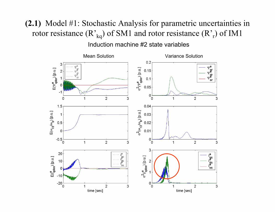
Induction machine #2 state variables
Variance SolutionMean Solution
(2.1) Model #1: Stochastic Analysis for parametric uncertainties inrotor resistance (R’kq) of SM1 and rotor resistance (R’r) of IM1

Excerpts from published emails in connection with shuttle Columbia’s last mission:
MOTIVATION OFMOTIVATION OFUNCERTAINTY QUANTIFICATION AND MANAGEMENTUNCERTAINTY QUANTIFICATION AND MANAGEMENT
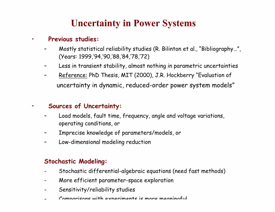
Uncertainty in Power Systems
• Previous studies:– Mostly statistical reliability studies (R. Bilinton et al., “Bibliography…”,
(Years: 1999,’94,’90,’88,’84,’78,’72)– Less in transient stability, almost nothing in parametric uncertainties– Reference: PhD Thesis, MIT (2000), J.R. Hockberry “Evaluation of
uncertainty in dynamic, reduced-order power system models”
• Sources of Uncertainty:– Load models, fault time, frequency, angle and voltage variations,
operating conditions, or– Imprecise knowledge of parameters/models, or– Low-dimensional modeling reduction
Stochastic Modeling:- Stochastic differential-algebraic equations (need fast methods)- More efficient parameter-space exploration- Sensitivity/reliability studies- Comparisons with experiments is more meaningful
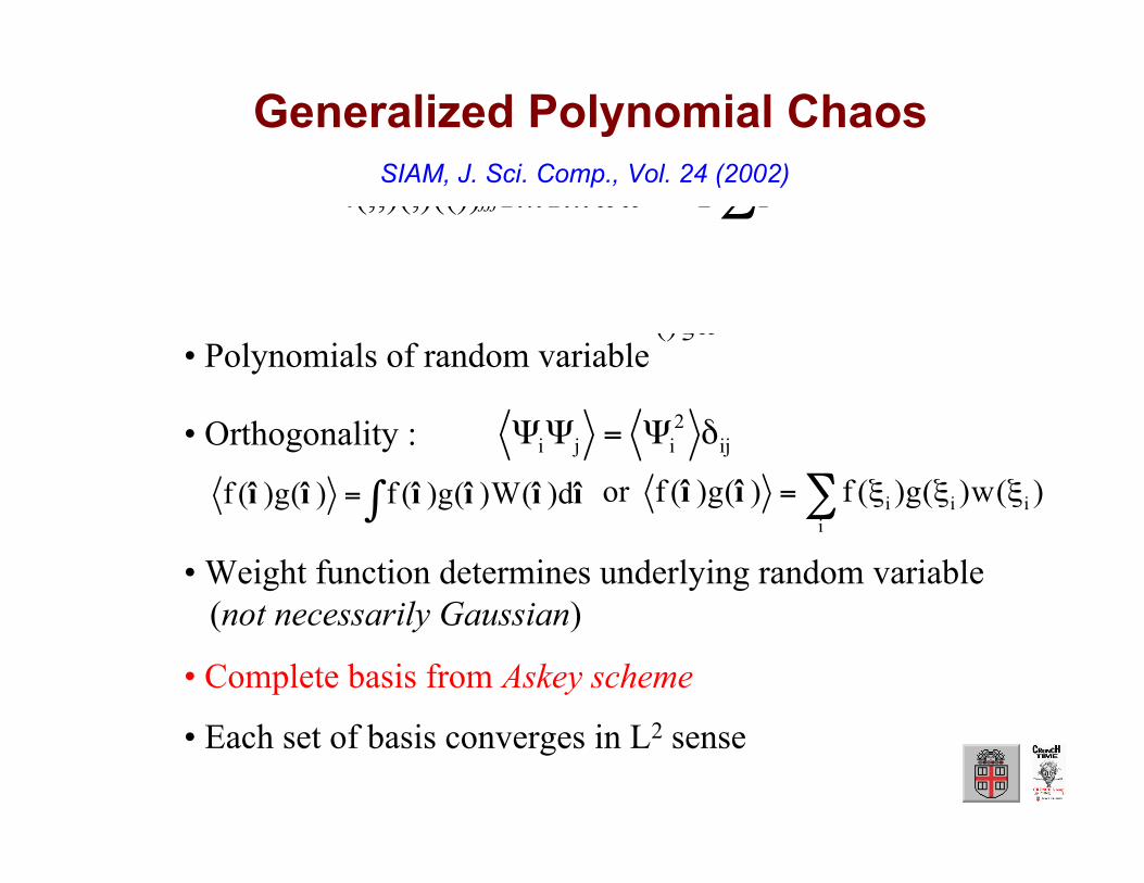
Generalized Polynomial ChaosSIAM, J. Sci. Comp., Vol. 24 (2002)
0(,;)(,)(())jjjTxtTxtωω∞==Ψ∑î
• Orthogonality : ij2iji δΨ=ΨΨ
∫= îîîîîî d)(W)(g)(f)(g)(f
• Weight function determines underlying random variable (not necessarily Gaussian)
• Complete basis from Askey scheme
• Polynomials of random variable()ξω
• Each set of basis converges in L2 sense
∑ ξξξ=i
iii )(w)(g)(f)(g)(f or îî
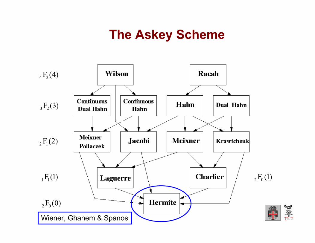
The Askey Scheme
)0(F02
)1(F02)1(F11
)2(F12
)3(F23
)4(F34
Wiener, Ghanem & Spanos
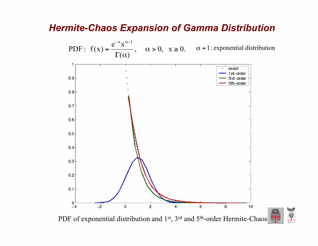
Hermite-Chaos Expansion of Gamma Distribution
PDF of exponential distribution and 1st, 3rd and 5th-order Hermite-Chaos
.0x ,0 ,)(
xe)x(f :PDF
1x
≥>ααΓ
=−α−
1=α : exponential distribution
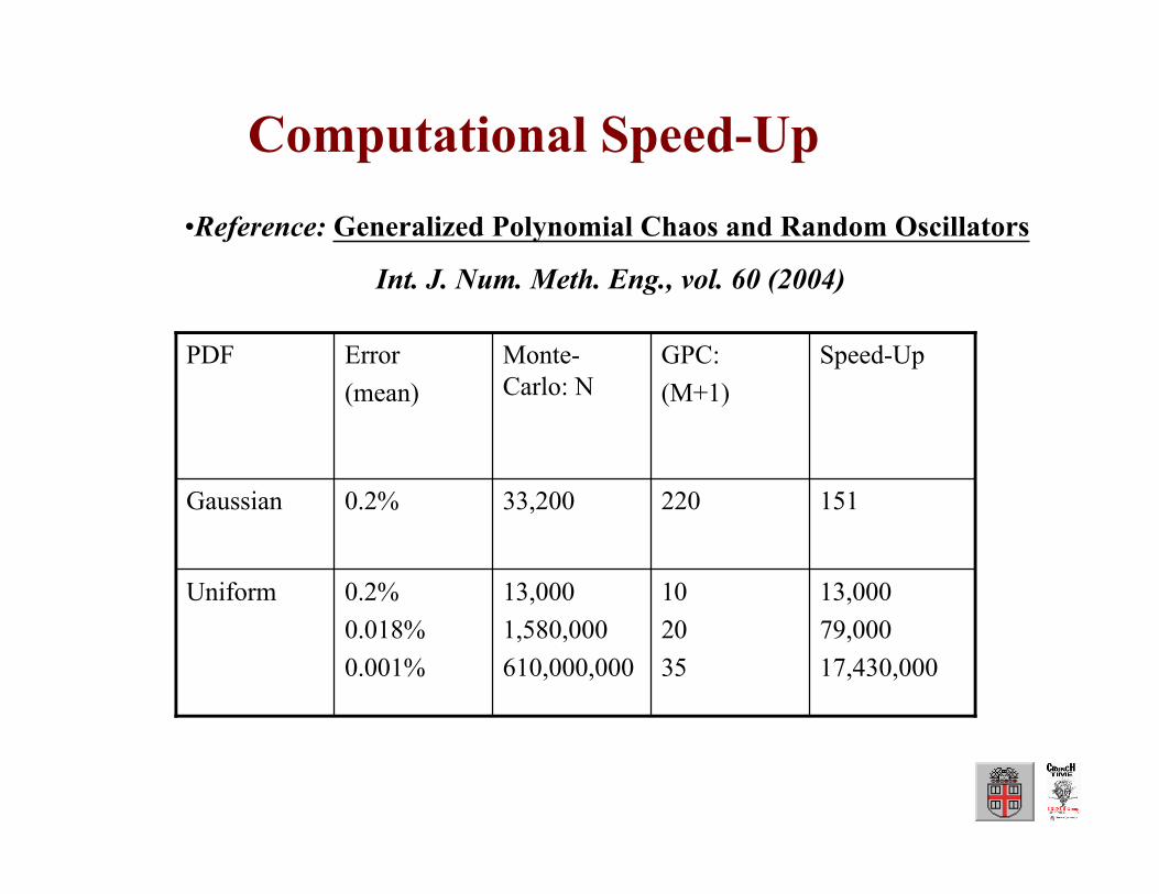
13,000
79,000
17,430,000
10
20
35
13,000
1,580,000
610,000,000
0.2%
0.018%
0.001%
Uniform
15122033,2000.2%Gaussian
Speed-UpGPC:
(M+1)
Monte-Carlo: N
Error
(mean)
Computational Speed-Up
•Reference: Generalized Polynomial Chaos and Random Oscillators
Int. J. Num. Meth. Eng., vol. 60 (2004)

Application to General Operator
• Galerkin projection
• Collocation projection
: number of grid points, such as quadrature points or sparse grids, etc.
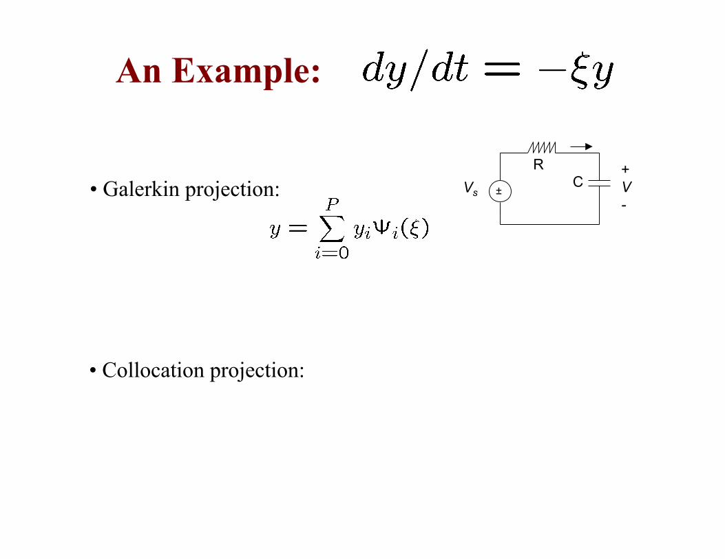
An Example:
• Galerkin projection:
• Collocation projection:
±
+V-
CR
Vs
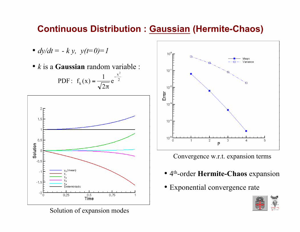
Continuous Distribution : Gaussian (Hermite-Chaos)
• dy/dt = - k y, y(t=0)=1
• k is a Gaussian random variable :
Solution of expansion modes
Convergence w.r.t. expansion terms
• 4th-order Hermite-Chaos expansion
• Exponential convergence rate
2x
k
2
e2
1)x(f :PDF
−
π=

Multi-Element gPC Method (ME-gPC):Random Decomposition
p.d.f.
1e 2e 3e
Assume that is defined on , where and are finite orinfinite in . We define a random decomposition as
ia ib[]1,diiiBab==×ξR
12,1,1,2,2,,112[,)[,)[,),,,if .kkkkkkdkdNkkkkBabababGBBBBkk==××===∅≠LUI
Random space is decomposed to smallelements as in finite element method.
p.d.f. is also decomposed similarly.
gPC on the whole random space will loseorthogonality in each random element for acertain random distribution.
ia ib
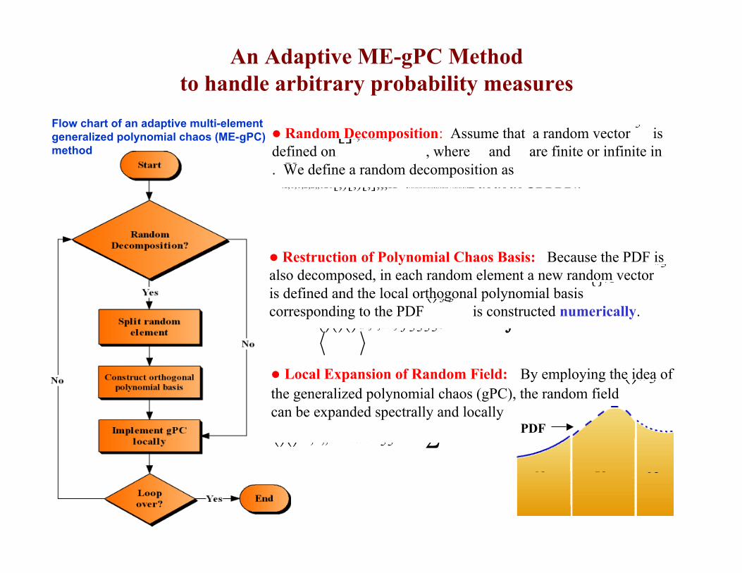
An Adaptive ME-gPC Methodto handle arbitrary probability measures
12,1,1,2,2,,121[,)[,)[,],,,if .kkkkkkdkdNkkkkBabababGBBBBkk==×××===∅≠LUI
Random Decomposition: Assume that a random vector isdefined on , where and are finite or infinite in. We define a random decomposition as
ia ib[]1,diiiBab==×ξ
R
Restruction of Polynomial Chaos Basis: Because the PDF isalso decomposed, in each random element a new random vectoris defined and the local orthogonal polynomial basiscorresponding to the PDF is constructed numerically.
kξ
()kfξ{}iΦ
()()()dkijikjkkkijBfξξξξδΦΦ=ΦΦ=∫
Flow chart of an adaptive multi-elementgeneralized polynomial chaos (ME-gPC)method
Local Expansion of Random Field: By employing the idea ofthe generalized polynomial chaos (gPC), the random fieldcan be expanded spectrally and locally
()uξ
()()01,2,,PkiikiuukNξξ==Φ=∑L
1e 2e 3e
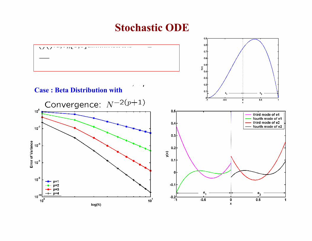
Stochastic ODE
()()0d,0,,[1,1]duuuutκωωκ=−=∈−
Case : Beta Distribution with1,2αβ==

Discontinuous Stochastic Solutions()()()()()()312231312110220330ddd,,2,ddd0;,0;,0;.xxxxxxxxxtttxxxxxxωωωωωω===−===
•gPC may fail for this problem due to discontinuities
101202303[1,1][1,1][1,1]xUxUxUξξξ=∈−=∈−=∈−

h-p Convergence and Adaptive Mesh
4.35e-61302.90e-4784.10e-3447.24e-228p=5
2.31e-52863.45e-41383.24e-3749.90e-236p=4
2.87e-58201.37e-42802.32e-31063.10e-246p=3
ErrorNErrorNErrorNErrorN
2110θ−= 4110θ−=3110θ−= 5110θ−=

(c): t=6
(b): t=3
(a): t=1
2D Adaptive Mesh for Discontinuous Solutions
Problem:
An accuracy of O(10-4) is maintained by adaptive meshes.
The elements are well refined around the discontinuous region ξ1=0.
The number of random elements increases almost linearly with time.
gPC fails to converge after a short-term integration.

Tie line or SM1’s current
Variance SolutionMean Solution
(2.1) Model #1: Stochastic Analysis for parametric uncertainties inrotor resistance (R’kq) of SM1 and rotor resistance (R’r) of IM1

•D. Xiu and G.E. Karniadakis, “The Wiener-Askey polynomial chaos for stochastic differentialequations”, SIAM J. Sci. Comput., vol. 24(2), pp. 619-644, 2002.
•D. Xiu and G.E. Karniadakis, “Modeling uncertainty in flow simulations via GeneralizedPolynomial Chaos”, J. Comp. Phys., vol. 87, pp. 137-167, 2003.
• D. Xiu and G.E. Karniadakis, “Modeling uncertainty in steady state diffusion problems viaGeneralized Polynomial Chaos”, Comput. Meth. Appl. Mech. Eng., vol 191, pp. 4927-4948, 2002.
• D. Lucor and G.E. Karniadakis, “Adaptive generalized polynomial chaos for nonlinear randomoscillators", SIAM J. Sci. Comput., vol. 26(2), pp. 720-735, 2004.
• X. Wan and G.E. Karniadakis, “An adaptive multi-element generalized polynomial chaosmethod for stochastic differential equations", J. Comp. Phys., vol. 209(2), pp. 617-642, 2005.
•X. Wan and G.E. Karniadakis, “Beyond Wiener-Askey expansions: Handling arbitrary PDFs",
Journal of Scientific Computing, in press.
•X. Wan and G.E. Karniadakis, “Multi-element generalized polynomial chaos for arbitraryprobability measures”, SIAM J. Sci. Comput., in press, 2006.
•X. Wan and G.E. Karniadakis, “Long-term behavior of polynomial chaos in stochastic flowsimulations", Comput. Methods Appl. Mech. Engrg., in press, 2006.
References on Stochastic Modeling

Comparison of Cost between MC and ME-gPC
Only h-convergence, N-2(p+1), is considered. N is the random element number along onerandom dimension and p is the polynomial chaos order.
For the same accuracy and different random dimension numbers, the lines show thecases where the cost of standard Monte Carlo is equal to that of ME-gPC. For a certainrandom dimension number, the region below the line is where MC wins; the region abovethe line is where ME-gPC wins.
Cost of MC:
Cost of ME-gPC:
h-convergence of ME-gPC:
For the same accuracy:
•Babuska, Tempone & Zouraris, SIAM J. Numer. Anal., vol. 42, 2005
•Schwab & Todor, Num. Math., vol. 95, 2003
High-Order Collocation Method

Sparse Grids