Multi-Criteria Decision Analysis - The Eye Various/multi-criteria_decision... · 3.3.2 Assessment...
299
Multi-Criteria Decision Analysis www.it-ebooks.info
Transcript of Multi-Criteria Decision Analysis - The Eye Various/multi-criteria_decision... · 3.3.2 Assessment...

Multi-Criteria Decision Analysis
Methods and Software
Alessio Ishizaka
Reader in Decision Analysis, Portsmouth Business SchoolUniversity of Portsmouth, UK
Philippe Nemery
Senior Research Scientist, SAP Labs – China, Shanghai, PRC
www.it-ebooks.info

This edition first published 2013C© 2013 John Wiley & Sons, Ltd
Registered officeJohn Wiley & Sons Ltd, The Atrium, Southern Gate, Chichester, West Sussex, PO19 8SQ, UnitedKingdom
For details of our global editorial offices, for customer services and for information about how to applyfor permission to reuse the copyright material in this book please see our website at www.wiley.com.
The right of the author to be identified as the author of this work has been asserted in accordance with theCopyright, Designs and Patents Act 1988.
All rights reserved. No part of this publication may be reproduced, stored in a retrieval system, ortransmitted, in any form or by any means, electronic, mechanical, photocopying, recording or otherwise,except as permitted by the UK Copyright, Designs and Patents Act 1988, without the prior permission ofthe publisher.
Wiley also publishes its books in a variety of electronic formats. Some content that appears in print maynot be available in electronic books.
Designations used by companies to distinguish their products are often claimed as trademarks. All brandnames and product names used in this book are trade names, service marks, trademarks or registeredtrademarks of their respective owners. The publisher is not associated with any product or vendormentioned in this book.
Limit of Liability/Disclaimer of Warranty: While the publisher and author have used their best efforts inpreparing this book, they make no representations or warranties with respect to the accuracy orcompleteness of the contents of this book and specifically disclaim any implied warranties ofmerchantability or fitness for a particular purpose. It is sold on the understanding that the publisher is notengaged in rendering professional services and neither the publisher nor the author shall be liable fordamages arising herefrom. If professional advice or other expert assistance is required, the services of acompetent professional should be sought.
Library of Congress Cataloging-in-Publication Data
Ishizaka, Alessio.Multi-criteria decision analysis : methods and software / Alessio Ishizaka, Philippe Nemery.
pages cmIncludes bibliographical references and index.ISBN 978-1-119-97407-9 (cloth)1. Multiple criteria decision making. 2. Multiple criteria decision making–Data processing.
3. Decision support systems. I. Nemery, Philippe. II. Title.T57.95.I84 2013003′.56–dc23
2013004490
A catalogue record for this book is available from the British Library.
ISBN: 978-1-119-97407-9
Typeset in 10/12pt Times by Aptara Inc., New Delhi, India
1 2013
www.it-ebooks.info

Contents
Foreword xi
Acknowledgements xiii
1 General introduction 11.1 Introduction 11.2 Decision problems 31.3 MCDA methods 41.4 MCDA software 51.5 Selection of MCDA methods 51.6 Outline of the book 8References 9
Part I FULL AGGREGATION APPROACH 11
2 Analytic hierarchy process 132.1 Introduction 132.2 Essential concepts of AHP 13
2.2.1 Problem structuring 142.2.2 Priority calculation 162.2.3 Consistency check 182.2.4 Sensitivity analysis 19
2.3 AHP software: MakeItRational 202.3.1 Problem structuring 202.3.2 Preferences and priority calculation 212.3.3 Consistency check 222.3.4 Results 242.3.5 Sensitivity analysis 25
2.4 In the black box of AHP 272.4.1 Problem structuring 272.4.2 Judgement scales 282.4.3 Consistency 312.4.4 Priorities derivation 332.4.5 Aggregation 39
www.it-ebooks.info

vi CONTENTS
2.5 Extensions of AHP 402.5.1 Analytic hierarchy process ordering 412.5.2 Group analytic hierarchy process 442.5.3 Clusters and pivots for a large number of alternatives 482.5.4 AHPSort 50
References 54
3 Analytic network process 593.1 Introduction 593.2 Essential concepts of ANP 59
3.2.1 Inner dependency in the criteria cluster 603.2.2 Inner dependency in the alternative cluster 633.2.3 Outer dependency 643.2.4 Influence matrix 67
3.3 ANP software: Super Decisions 683.3.1 Problem structuring 693.3.2 Assessment of pairwise comparison 703.3.3 Results 733.3.4 Sensitivity analysis 74
3.4 In the black box of ANP 763.4.1 Markov chain 763.4.2 Supermatrix 78
References 80
4 Multi-attribute utility theory 814.1 Introduction 814.2 Essential concepts of MAUT 81
4.2.1 The additive model 834.3 RightChoice 89
4.3.1 Data input and utility functions 894.3.2 Results 934.3.3 Sensitivity analysis 944.3.4 Group decision and multi-scenario analysis 95
4.4 In the black box of MAUT 974.5 Extensions of the MAUT method 98
4.5.1 The UTA method 984.5.2 UTAGMS 1054.5.3 GRIP 111
References 112
5 MACBETH 1145.1 Introduction 1145.2 Essential concepts of MACBETH 114
5.2.1 Problem structuring: Value tree 115
www.it-ebooks.info

CONTENTS vii
5.2.2 Score calculation 1175.2.3 Incompatibility check 118
5.3 Software description: M-MACBETH 1225.3.1 Problem structuring: Value tree 1225.3.2 Evaluations and scores 1225.3.3 Incompatibility check 1255.3.4 Results 1275.3.5 Sensitivity analysis 1275.3.6 Robustness analysis 127
5.4 In the black box of MACBETH 1315.4.1 LP-MACBETH 1315.4.2 Discussion 133
References 133
Part II OUTRANKING APPROACH 135
6 PROMETHEE 1376.1 Introduction 1376.2 Essential concepts of the PROMETHEE method 137
6.2.1 Unicriterion preference degrees 1386.2.2 Unicriterion positive, negative and net flows 1426.2.3 Global flows 1436.2.4 The Gaia plane 1466.2.5 Sensitivity analysis 148
6.3 The Smart Picker Pro software 1496.3.1 Data entry 1496.3.2 Entering preference parameters 1516.3.3 Weights 1536.3.4 PROMETHEE II ranking 1556.3.5 Gaia plane 1576.3.6 Sensitivity analysis 158
6.4 In the black box of PROMETHEE 1606.4.1 Unicriterion preference degrees 1626.4.2 Global preference degree 1636.4.3 Global flows 1646.4.4 PROMETHEE I and PROMETHEE II ranking 1666.4.5 The Gaia plane 1676.4.6 Influence of pairwise comparisons 168
6.5 Extensions of PROMETHEE 1706.5.1 PROMETHEE GDSS 1706.5.2 FlowSort: A sorting or supervised classification method 172
References 177
7 ELECTRE 1807.1 Introduction 180
www.it-ebooks.info

viii CONTENTS
7.2 Essentials of the ELECTRE methods 1807.2.1 ELECTRE III 183
7.3 The Electre III-IV software 1897.3.1 Data entry 1907.3.2 Entering preference parameters 1917.3.3 Results 193
7.4 In the black box of ELECTRE III 1947.4.1 Outranking relations 1947.4.2 Partial concordance degree 1957.4.3 Global concordance degree 1967.4.4 Partial discordance degree 1967.4.5 Outranking degree 1977.4.6 Partial ranking: Exploitation of the outranking relations 1997.4.7 Some properties 203
7.5 ELECTRE-Tri 2047.5.1 Introduction 2047.5.2 Preference relations 2057.5.3 Assignment rules 2077.5.4 Properties 207
References 210
Part III GOAL, ASPIRATION OR REFERENCE-LEVELAPPROACH 213
8 TOPSIS 2158.1 Introduction 2158.2 Essentials of TOPSIS 215References 221
9 Goal programming 2229.1 Introduction 2229.2 Essential concepts of goal programming 2229.3 Software description 227
9.3.1 Microsoft Excel Solver 2279.4 Extensions of the goal programming 228
9.4.1 Weighted goal programming 2289.4.2 Lexicographic goal programming 2309.4.3 Chebyshev goal programming 232
References 234
10 Data Envelopment Analysis 235Jean-Marc Huguenin
10.1 Introduction 23510.2 Essential concepts of DEA 236
10.2.1 An efficiency measurement method 236
www.it-ebooks.info

CONTENTS ix
10.2.2 A DEA case study 23710.2.3 Multiple outputs and inputs 24710.2.4 Types of efficiency 24810.2.5 Managerial implications 249
10.3 The DEA software 25210.3.1 Building a spreadsheet in Win4DEAP 25410.3.2 Running a DEA model 25510.3.3 Interpreting results 257
10.4 In the black box of DEA 26210.4.1 Constant returns to scale 26310.4.2 Variable returns to scale 266
10.5 Extensions of DEA 26810.5.1 Adjusting for the environment 26810.5.2 Preferences 26810.5.3 Sensitivity analysis 26910.5.4 Time series data 270
References 270
Part IV INTEGRATED SYSTEMS 275
11 Multi-method platforms 27711.1 Introduction 27711.2 Decision Deck 27811.3 DECERNS 278
11.3.1 The GIS module 27911.3.2 The MCDA module 28111.3.3 The GDSS module 28411.3.4 Integration 286
References 287
Appendix: Linear optimization 288A.1 Problem modelling 288A.2 Graphical solution 289A.3 Solution with Microsoft Excel 289
Index 293
www.it-ebooks.info

Foreword
The growing recognition that decision makers will often try to achieve multiple, andusually conflicting, objectives has led during the last three decades to the developmentof multi-criteria decision analysis (MCDA). This is now a vast field of research, withits scientific community and its specialized journals, as well as a large and growingnumber of real-world applications, for supporting both public policy making anddecisions by private corporations.
Students and practitioners coming to the field, however, will be surprised by theplethora of alternative methods, overloaded by the array of software available, andpuzzled by the diversity of approaches that an analyst needs to choose from. Forprecisely these reasons, this book is a very welcome event for the field. AlessioIshizaka and Philippe Nemery have managed to provide an accessible, but rigorous,introduction to the main existing MCDA methods available in the literature.
There are several features of the book that are particularly innovative. First, itprovides a balanced assessment of each method, and positions them in terms of thetype of evaluation that the decision requires (a single choice among alternatives, theranking of all alternatives, the sorting of alternatives into categories, or the descriptionof consequences) and the level of preference information that each method requires(from utility functions to no preference information). This taxonomy helps bothresearchers and practitioners in locating adequate methods for the problems theyneed to analyze.
Second, the methods are presented with the right level of formulation and axiom-atization for an introductory course. This makes the book accessible to anyone witha basic quantitative background. Readers who wish to learn in greater depth about aparticular method can enjoy the more advanced content covered ‘in the black box’ ofeach chapter.
Third, the book illustrates each method with widely available and free software.This has two major benefits. Readers can easily see how the method works in practicevia an example, consolidating the knowledge and the theoretical content. They canalso reflect on how the method could be used in practice, to facilitate real-worlddecision-making processes.
Fourth, instructors using the book, as well as readers, can benefit from the com-panion website (www.wiley.com/go/multi criteria decision analysis) andthe availability of software files and answers to exercises.
www.it-ebooks.info

xii FOREWORD
This book should therefore be useful reading for anyone who wants to learnmore about MCDA, or for those MCDA researchers who want to learn more aboutother MCDA methods and how to use specialized software to support multi-criteriadecision making.
Gilberto MontibellerDepartment of Management
London School of Economics
www.it-ebooks.info

Acknowledgements
We are indebted to Kimberley Perry for her patience and constructive feedback whilereviewing the manuscript. We would like to thank Ian Stevens and Alfred Quintano,who proofread a chapter.
We wish to express our sincere gratitude to Prof. Roman Słowinski, Poznan Uni-versity of Technology; Dawid Opydo, BS Consulting Dawid Opydo; Tony Kennedy,Ventana Systems UK; Prof. Boris Yatsalo and Dr Sergey Gritsyuk for their sugges-tions.
We are grateful to the following organizations which granted us the permission toreproduce screenshots of their software: BS Consulting Dawid Opydo, Creative Deci-sion Foundations, Ventana Systems UK Ltd, Lamsade Universite Paris-Dauphine,Poznan University of Technology, BANA Consulting Lda, Smart-Picker, ObninskState Technical University of Nuclear Power Engineering, Prof. Tim Coelli (TheUniversity of Queensland), Prof. Michel Deslierres (Univeriste de Moncton).
Last, but not least, we would like to thank all our students who have provided uswith constant feedback and new ideas.
www.it-ebooks.info
1
General introduction
1.1 Introduction
People face making decisions both in their professional and private lives. A managerin a company, for example, may need to evaluate suppliers and develop partnershipswith the best ones. A household may need to choose an energy supplier for theirfamily home. Students cannot ignore university rankings. Often candidates for a jobvacancy are ‘ranked’ based on their experience, performance during the interview,etc.As well as ranking and choice problems, there are also classification problems
that have existed since classical times. In the fourth century bc, the ancient Greekphilosopher Epicurus arranged human desires into two classes: vain desires (e.g.the desire for immortality) and natural desires (e.g. the desire for pleasure). Theseclassifications were supposed to help in finding inner peace. Nowadays, classificationproblems occur naturally in daily life. A doctor, for instance, diagnoses a patienton the basis of their symptoms and assigns them to a pathology class to be ableto prescribe the appropriate treatment. In enterprise, projects are often sorted intopriority-based categories. Not long ago, a study showed that over 20millionBrazilianshave moved from the lower social categories (D and E) to category C, the firsttier of the middle class, and are now active consumers due to an increase in legalemployment (Observador 2008). Hurricanes or cyclones are sorted into one of thefive Saffir–Simpson categories based on their wind speed, superficial pressure andtide height.All of these examples show that delicate decision problems arise frequently.
Decision problems such as ranking, choice and sorting problems are often complex asthey usually involve several criteria. People no longer consider only one criterion (e.g.price) when making a decision. To build long-term relationships, make sustainableand environmentally friendly decisions, companies consider multiple criteria in theirdecision process.
Multi-Criteria Decision Analysis: Methods and Software, First Edition. Alessio Ishizaka and Philippe Nemery.© 2013 John Wiley & Sons, Ltd. Published 2013 by John Wiley & Sons, Ltd.
www.it-ebooks.info

2 MULTI-CRITERIA DECISION ANALYSIS
Table 1.1 Category of decision problems.
Decision Time perspective Novelty Degree of structure Automation
Strategic long term new low lowTactical medium term adaptive semi-structured middleOperational short term every day well defined high
Most of the time, there is no one, perfect option available to suit all the criteria:an ‘ideal’ option does not usually exist, and therefore a compromise must be found.To address this problem the decision maker can make use of naıve approaches suchas a simple weighted sum. The weighted sum, described in Section 4.3.1, is a specialcase of a more complex method and can only be applied with the right precautions(correct normalization phase, independent criteria, etc.) to enable sensible outputs.In reality, this approach is unrefined as it assumes linearity of preferences which maynot reflect the decision maker’s preferences. For example, it cannot be assumed that awage of £4000 is twice as good as one of £2000. Some people would see their utilityof preference improved by a factor of 5 with a wage of £4000. This cannot always bemodelled with a weighted sum.Multi-criteria decision analysis (MCDA)methods have been developed to support
the decision maker in their unique and personal decision process. MCDA methodsprovide stepping-stones and techniques for finding a compromise solution. They havethe distinction of placing the decision maker at the centre of the process. They are notautomatable methods that lead to the same solution for every decision maker, but theyincorporate subjective information. Subjective information, also known as preferenceinformation, is provided by the decision maker, which leads to the compromisesolution.MCDA is a discipline that encompasses mathematics, management, informatics,
psychology, social science and economics. Its application is even wider as it can beused to solve any problem where a significant decision needs to be made. Thesedecisions can be either tactical or strategic, depending on the time perspective of theconsequences (Table 1.1).A large number of methods have been developed to solve multi-criteria problems.
This development is ongoing (Wallenius et al. 2008) and the number of academicMCDA-related publications is steadily increasing. This expansion is among othersdue to both the efficiency of researchers and the development of specific methods forthe different types of problem encountered inMCDA. The software available, includ-ing spreadsheets containing method computations, ad hoc implementations, off-the-shelf, web or smartphone applications, has made MCDA methods more accessibleand contributed to the growth in use of MCDA methods amongst researchers and theuser community.The aim of this book is to make MCDA methods even more intelligible to
novice users such as students, or practitioners, but also to confirmed researchers.This book is ideal for people taking the first step into MCDA or specific MCDAmethods. The cases studies and exercises effectively combine the mathematical and
www.it-ebooks.info

GENERAL INTRODUCTION 3
practical approach. For each method described in this book, an intuitive explanationand interpretation of the method is set out, followed by a detailed description ofthe software best suited to the method. Free or free trial version software has beenintentionally chosen, as it allows the reader to better understand the main ideasbehind the methods by practising with the exercises in this book. Furthermore, theuser has access to a Microsoft Excel spreadsheet containing an ‘implementation’ ofeach method. Software files and answers to the exercises can be downloaded from thecompanion website, indicated by the icon in the book. The selected software andexercises allow the user to observe the impact of changes to the data on the results.The use of software enables the decision maker or analyst to communicate and justifydecisions in a systematic way.Each chapter contains a section (‘In the black box’) where scientific references
and further reading are indicated for those interested in a more in-depth descriptionor detailed understanding of the methods. Each chapter concludes with extensions ofthe methods to other decision problems, such as group decision or sorting problems.This first chapter describes the different type of decision problems to be addressed
in this book. This is followed by the introduction of the MCDA method best suitedto solving these problems along with the corresponding software implementation.As several methods can solve similar problems, a section devoted to choosing anappropriate method has also been included. The chapter concludes with an outline ofthe book.
1.2 Decision problems
On any one day people face a plethora of different decisions. However, Roy (1981)has identified four main types of decision:
1. The choice problem. The goal is to select the single best option or reduce thegroup of options to a subset of equivalent or incomparable ‘good’ options. Forexample, a manager selecting the right person for a particular project.
2. The sorting problem. Options are sorted into ordered and predefined groups,called categories. The aim is to then regroup the optionswith similar behavioursor characteristics for descriptive, organizational or predictive reasons. Forinstance, employees can be evaluated for classification into different cate-gories such as ‘outperforming employees’, ‘average-performing employees’and ‘weak-performing emplyees’. Based on these classifications, necessarymeasures can be taken. Sorting methods are useful for repetitive or automaticuse. They can also be used as an initial screening to reduce the number ofoptions to be considered in a subsequent step.
3. The ranking problem. Options are ordered from best to worst by means ofscores or pairwise comparisons, etc. The order can be partial if incomparableoptions are considered, or complete. A typical example is the ranking ofuniversities according to several criteria, such as teaching quality, researchexpertise and career opportunities.
www.it-ebooks.info

4 MULTI-CRITERIA DECISION ANALYSIS
4. The description problem. The goal is to describe options and their conse-quences. This is usually done in the first step to understand the characteristicsof the decision problem.
Additional problem types have also been proposed in the MCDA community:
5. Elimination problem. Bana e Costa (1996) proposed the elimination problem,a particular branch of the sorting problem.
6. Design problem. The goal is to identify or create a new action, which willmeet the goals and aspirations of the decision maker (Keeney 1992)
To this list of problems the ‘elicitation problem’ can be added as it aims to elicitthe preference parameters (or subjective information) for a specific MCDA method.Moreover, when the problem involves several decision makers, an appropriate groupdecision method needs to be used.Many other decision problems exist, often combining several of the problems
listed above. However, this book concentrates on the first four decision problems andpresents extensions of some of the methods that allow, for example, group, elicitationand description problems also to be addressed.
1.3 MCDA methods
To solve the problems defined in the previous section, ad hoc methods have beendeveloped. In this book, the most popular MCDA methods are described along withtheir variants. Table 1.2 presents these methods and the decision problems they solve.There are many more decision methods than those presented in Table 1.2, but thisbook confines itself to the most popular methods that have a supporting softwarepackage.
Table 1.2 MCDA problems and methods.
Choice Ranking Sorting DescriptionChapter problems problems problems problems
2 AHP AHP AHPSort3 ANP ANP4 MAUT/UTA MAUT/UTA UTADIS5 MACBETH MACBETH6 PROMETHEE PROMETHEE FlowSort GAIA, FS-Gaia7 ELECTRE I ELECTRE III ELECTRE-Tri8 TOPSIS TOPSIS9 Goal Programming10 DEA DEA11 Multi-methods platform that supports various MCDA methods
www.it-ebooks.info

GENERAL INTRODUCTION 5
Table 1.3 MCDA software programs.
Problems MCDA Methods Software
Ranking, description,choice
PROMETHEE – GAIA Decision Lab,D-Sight, Smart Picker Pro,Visual Promethee
Ranking, choice PROMETHEE DECERNSELECTRE Electre IS, Electre III-IVUTA Right Choice, UTA+, DECERNSAHP MakeItRational, ExpertChoice,
Decision Lens, HIPRE 3+,RightChoiceDSS, Criterium,EasyMind, Questfox,ChoiceResults, 123AHP,DECERNS
ANP Super Decisions, Decision LensMACBETH M-MACBETHTOPSIS DECERNSDEA Win4DEAP, Efficiency
Measurement System, DEASolver Online, DEAFrontier,DEA-Solver PRO, FrontierAnalyst
Choice Goal Programming -Sorting, description FlowSort - FS-GAIA Smart Picker ProSorting ELECTRE-Tri Electre Tri, IRIS
UTADIS -AHPSort -
1.4 MCDA software
Researchers and commercial companies have developed various software programsover the last decade to help users structure and solve their decision problems. The aimof this book is not to describe all existing software, but to narrow the list down to thepackages that apply to the methods described. A non-exhaustive list of the programsavailable is given in Table 1.3. The software packages represented in this book are inbold. Let us remark that the user has access to all the Microsoft Excel spreadsheetson the companion website.
1.5 Selection of MCDA methods
Considering the number of MCDA methods available, the decision maker is facedwith the arduous task of selecting an appropriate decision support tool, and often
www.it-ebooks.info

6 MULTI-CRITERIA DECISION ANALYSIS
the choice can be difficult to justify. None of the methods are perfect nor can theybe applied to all problems. Each method has its own limitations, particularities,hypotheses, premises and perspectives. Roy and Bouyssou (1993) say that ‘althoughthe great diversity of MCDA procedures may be seen as a strong point, it can alsobe a weakness. Up to now, there has been no possibility of deciding whether onemethod makes more sense than another in a specific problem situation. A systematicaxiomatic analysis of decision procedures and algorithms is yet to be carried out.’Guitouni et al. (1999) propose an initial investigative framework for choos-
ing an appropriate multi-criteria procedure; however, this approach is intended forexperienced researchers. The next paragraphs give some guidance on selecting anappropriate method according to the decision problem, which will avoid an arbitraryadoption process.There are different ways of choosing appropriateMCDAmethods to solve specific
problems. One way is to look at the required input information, that is, the data andparameters of the method and consequently the modelling effort, as well as lookingat the outcomes and their granularity (Tables 1.4 and 1.5). This approach is supportedby Guitouni et al. (1999).If the ‘utility function’ for each criterion (a representation of the perceived utility
given the performance of the option on a specific criterion) is known, then MAUT(Chapter 4) is recommended.However, the construction of the utility function requiresa lot of effort, but if it is too difficult there are alternatives. Another way is by usingpairwise comparisons between criteria and options. AHP (Chapter 2) andMACBETH(Chapter 5) support this approach. The difference is that comparisons are evaluatedon a ratio scale for AHP and on an interval scale for MACBETH. The decision makerneeds to know which scale is better suited to yield their preferences. The drawbackis that a large quantity of information is needed.Another alternative way is to define key parameters. For example, PROMETHEE
(Chapter 6) only requires indifference and preference thresholds, whilst ELECTRE(Chapter 7) requires indifference, preference and veto thresholds. There exist so-called elicitation methods to help defining these parameters, but if the user wants toavoid those methods or parameters, TOPSIS (Chapter 8) can be used because onlyideal and anti-ideal options are required. If criteria are dependent, ANP (Chapter 3)or the Choquet integral1 can be used.The modelling effort generally defines the richness of the output. One advantage
to defining utility functions is that the options of the decision problem have a globalscore. Based on this score, it is possible to compare all options and rank them frombest to worst, with equal rankings permitted. This is defined as a complete ranking.This approach is referred to as the full aggregation approach where a bad score onone criterion can be compensated by a good score on another criterion.Outranking methods are based on pairwise comparisons. This means that the
options are compared two-by-two by means of an outranking or preference degree.The preference or outranking degree reflects how much better one option is than
1 This method has not been described in this book because it is not supported by a software package.
www.it-ebooks.info

Table 1.4 Required inputs for MCDA ranking or choice method.
tuptuOdohtemADCMtupnitroffEstupnI
Ran
king
/choice
prob
lem
HGIHyreVnoitcnufytilitu MAUT Complete ranking with scores
pairwise comparisons on a ratio scale
and interdependencies
ANP Complete ranking with scores
pairwise comparisons on an interval
scale
MACBETH Complete ranking with scores
pairwise comparisons on a ratio scale AHP Complete ranking with scores
indifference, preference and veto
thresholds
ELECTRE Partial and complete ranking
(pairwise outranking degrees)
indifference and preference thresholds PROMETHEE Partial and complete ranking (pairwise
preference degrees and scores)
ideal option and constraints Goal programming Feasible solution with deviation score
ideal and anti-ideal option TOPSIS Complete ranking with closeness
score
no subjective inputs required Very LOW DEA Partial ranking with effectiveness
score
www.it-ebooks.info

8 MULTI-CRITERIA DECISION ANALYSIS
Table 1.5 Required inputs for MCDA sorting methods.
Effort
Inputs Input MCDA method Output
Sortingmetho
d
utility function HIGH UTADIS Classification with
scoring
pairwise comparisons
on a ratio scale
AHPSort Classification with
scoring
indifference, preference
and veto thresholds
ELECTRE-TRI Classification with
pairwise outranking
degrees
indifference and
preference thresholds
LOW FLOWSORT Classification with
pairwise outranking
degrees and scores
another. It is possible for some options to be incomparable. The comparison betweentwo options is difficult as they have different profiles: one option may be better basedone set of criteria and the other better based on another set of criteria. These incom-parabilities mean that a complete ranking is not always possible, which is referred toas a partial ranking. The incomparability is a consequence of the non-compensatoryaspect of those methods. When facing a decision problem, it is important to definethe type of output required from the beginning (presented in Tables 1.4 and 1.5).Goal programming and data envelopment analysis (DEA) are also part of the
MCDA family but are used in special cases. In goal programming, an ideal goal canbe defined subject to feasibility constraints. DEA is mostly used for performanceevaluation or benchmarking, where no subjective inputs are required.
1.6 Outline of the book
Following this introduction, in which general concepts of MCDA are explained, ninechapters describe themajorMCDAmethods. Each chapter can be read independently,and they are grouped into three sections, according to their approach:
� Full aggregation approach (or American school). A score is evaluated for eachcriterion and these are then synthesized into a global score. This approachassumes compensable scores, i.e. a bad score for one criterion is compensatedfor by a good score on another.
� Outranking approach (or French school). A bad score may not be compensatedfor by a better score. The order of the options may be partial because the notionof incomparability is allowed. Two options may have the same score, but theirbehaviour may be different and therefore incomparable.
www.it-ebooks.info

GENERAL INTRODUCTION 9
� Goal, aspiration or reference level approach. This approach defines a goalon each criterion, and then identifies the closest options to the ideal goal orreference level.
Most chapters are divided into four sections, with the exception of specificMCDAmethods, as extensions do not exist. Specific objectives are as follows:
� Essential concepts. The reader will be able to describe the essentials of theMCDA method.
� Software. The reader will be able to solve MCDA problems using the corre-sponding software.
� In the black box. The readerwill understand the calculations behind themethod.An exercise in Microsoft Excel facilitates this objective.
� Extensions. The reader will be able to describe the extensions of the MCDAmethods to other decision problems, such as sorting or group decisions.
The book concludes with a description of the integrated software DECERNS,which incorporates six MCDA methods and a Geographical Information System.Linear programming, the underlying method for MACBETH and goal programming,is explained in the Appendix.
References
Bana e Costa, C. (1996). Les problematiques de l’aide a la decision: Vers l’enrichissement dela trilogie choix–tri–rangement. RAIRO – Operations Research, 30(2), 191–216.
Guitouni, A., Martel, J., and Vincke, P. (1999). A framework to choose a discretemulticriterionaggregation procedure. Technical Report.
Keeney, R. (1992). Value-Focused Thinking: A Path to Creative Decision Making. Cambridge,MA: Harvard University Press.
Observador (2008). The growth of class ‘C’ and its electoral importance. Observador, 31March, p. 685.
Roy, B. (1981). The optimisation problem formulation: Criticism and overstepping. Journalof the Operational Research Sociey, 32(6), 427–436.
Roy, B., and Bouyssou, D. (1993). Aide multicritere a la decision: Methodes et cas. Paris:Economica.
Wallenius, J. D., Dyer, J.S., Fishburn, P.C., Steuer, R.E., Zionts, S., and Deb, K. (2008).Multiple criteria decision making, multiattribute utility theory: Recent accomplishmentsand what lies ahead. Management Science, 54(7), 1336–1349.
www.it-ebooks.info

Part I
FULL AGGREGATIONAPPROACH
Multi-Criteria Decision Analysis: Methods and Software, First Edition. Alessio Ishizaka and Philippe Nemery.© 2013 John Wiley & Sons, Ltd. Published 2013 by John Wiley & Sons, Ltd.
www.it-ebooks.info

2
Analytic hierarchy process
2.1 Introduction
This chapter explains the theory behind and practical uses of the analytic hierarchyprocess (AHP) method as well as its extensions. MakeItRational, a software packagethat helps to structure problems and calculate priorities using AHP, is described.Section 2.3 is designed for readers interested in the methodological background ofAHP. Section 2.4 covers the extensions of AHP in group decision, sorting, scenarioswith incomparability and large size problems.
The companion website provides illustrative examples with Microsoft Excel, andcase studies and examples with MakeItRational.
2.2 Essential concepts of AHP
AHP was developed by Saaty (1977, 1980). It is a particularly useful method whenthe decision maker is unable to construct a utility function, otherwise MAUT isrecommended (Chapter 4). To use AHP the user needs to complete four steps toobtain the ranking of the alternatives. As with any other MCDA method, the problemfirst has to be structured (Section 2.2.1). Following this, scores – or priorities, as theyare known in AHP – are calculated based on the pairwise comparisons provided bythe user (Section 2.2.2). The decision maker does not need to provide a numericaljudgement; instead a relative verbal appreciation, more familiar to our daily live, issufficient. There are two additional steps that can be carried out: a consistency check(Section 2.2.3) and a sensitivity analysis (Section 2.2.4). Both steps are optional butrecommended as confirmation of the robustness of the results. The consistency checkis common in all methods based on pairwise comparisons like AHP. The supportingsoftware of MakeItRational facilitates the sensitivity analysis.
Multi-Criteria Decision Analysis: Methods and Software, First Edition. Alessio Ishizaka and Philippe Nemery.© 2013 John Wiley & Sons, Ltd. Published 2013 by John Wiley & Sons, Ltd.
www.it-ebooks.info

14 MULTI-CRITERIA DECISION ANALYSIS
2.2.1 Problem structuring
AHP is based on the motto divide and conquer. Problems that require MCDA tech-niques are complex and, as a result, it is advantageous to break them down and solveone ‘sub-problem’ at a time. This breakdown is done in two phases of the decisionprocess during:
� the problem structuring and
� the elicitation of priorities through pairwise comparisons.
The problem is structured according to a hierarchy (e.g. Figure 2.2) where the topelement is the goal of the decision. The second level of the hierarchy represents thecriteria, and the lowest level represents the alternatives. In more complex hierarchies,more levels can be added. These additional levels represent the sub-criteria. In anycase, there are a minimum of three levels in the hierarchy.
Throughout this chapter, a shop location problem (Case Study 2.1) will be con-sidered to illustrate the different steps of the AHP process.
Case Study 2.1
A businessman wants to open a new sports shop in one of three different locations:
(a) A shopping centre. The shopping centre has a high concentration of avariety of shops and restaurants. It is a busy area, with a mix of customersand people walking around. Shops regularly use large displays and pro-motions to attract potential customers. As demand for these retail units islow, the rental costs are reasonable.
(b) The city centre. The city centre is a busy area, and a meeting point forboth young people and tourists. Attractions such as dance shows, clownsand market stalls are often organized, which attract a variety of visitors.The city centre has several small shops located at ground level in historicalbuildings, which suggests high rental costs. These shops have a highnumber of customers and are often in competition.
(c) A new industrial area. The new industrial estate is in the suburbs of thecity, where several businesses have recently been set up. Some buildingshave been earmarked for small shops, but on the whole it has been dif-ficult to attract tenants, which means that rental costs are currently low.Customers of the existing shops mainly work in the area and only a fewcustomers come from the surrounding towns or cities to shop here.
Given the description of the problem, four criteria will be considered in makingthe final decision (Table 2.1).
www.it-ebooks.info

ANALYTIC HIERARCHY PROCESS 15
Table 2.1 Criteria for shop location decision.
Criterion Explanation
Visibility Probability that a random passer-by notices the shopCompetition Level of competition in the areaFrequency Average number of customers in similar shops in the areaRental cost Average rental cost by square metre
Figure 2.1 represents the hierarchy of Case Study 2.1. It has three levels, the min-imum required to solve a problem with AHP. Other sub-criteria could be considered,for example, the competition criterion could be broken down into two sub-criteria:direct and indirect competition. Direct competition would be the number of othersports shops. Indirect competition would represent other types of shop, which coulddistract potential customers. To keep the example simple, additional levels will notbe considered at this stage.
Each lower level is prioritized according to its immediate upper level. The appro-priate question to ask with regard to prioritization depends on the context and some-times on the decision maker. For example, in order to prioritize the criteria of level2 with regard to the goal ‘location of a sports shop’, an appropriate question wouldbe: ‘Which criterion is most important for choosing the location of the sports shopand to what extent?’ On the other hand, the alternatives in level 3 must be prioritizedwith regard to each criterion in level 2. In this case, an appropriate question would
Location of asports shop
Visibility
Industrial area
Shopping centre
City centre
Competition
Industrial area
Shopping centre
City centre
Frequency
Industrial area
Shopping centre
City centre
Rental cost
Industrial area
Shopping centre
City centre
Level 3
Level 2
Level 1
Figure 2.1 Hierarchy of decision levels for Case Study 2.1.
www.it-ebooks.info

16 MULTI-CRITERIA DECISION ANALYSIS
Location of asports shop
Visibility Competition
Industrial area Shopping centre City centre
Frequency Rental cost
Level 3
Level 2
Level 1
Figure 2.2 Traditional representation of the hierarchy.
be: ‘Which alternative is preferable to fulfil the given criterion and to what extent?’In Case Study 2.1, five different prioritizations are required:
� four local prioritizations of alternatives with regard to each criterion and
� one criteria prioritization.
The aggregation of the local and criteria prioritizations leads to global prioritizations.As Figure 2.1 contains redundant information at the lowest level, the alternatives
in the hierarchy are often not repeated or are connected as in Figure 2.2.
2.2.2 Priority calculation
A priority is a score that ranks the importance of the alternative or criterion in thedecision. Following the problem-structuring phase (see Section 2.2.1), three types ofpriorities have to be calculated:
� Criteria priorities. Importance of each criterion (with respect to the top goal).
� Local alternative priorities. Importance of an alternative with respect to onespecific criterion.
� Global alternative priorities. Priority criteria and local alternative prioritiesare intermediate results used to calculate the global alternative priorities. Theglobal alternative priorities rank alternatives with respect to all criteria andconsequently the overall goal.
The criteria and local alternatives priorities are calculated using the same tech-nique. Instead of directly allocating performances to alternatives (or criteria) as inthe other techniques from the American school (see MAUT, Chapter 4), AHP uses
www.it-ebooks.info

ANALYTIC HIERARCHY PROCESS 17
Table 2.2 The 1–9 fundamental scale.
Degree of importance Definition
1 Equal importance2 Weak3 Moderate importance4 Moderate plus5 Strong importance6 Strong plus7 Very strong or demon-strated importance8 Very, very strong9 Extreme importance
pairwise comparisons. Psychologists often use this technique (Yokoyama 1921; Thur-stone 1927), for example, to evaluate the food preference of a cat by presenting twodishes at a time. The cat indicates its preference by eating one dish. The psycholo-gists argue that it is easier and more accurate to express a preference between onlytwo alternatives than simultaneously among all the alternatives. The use of pairwisecomparisons (called paired comparisons by psychologists) is generally evaluated onthe fundamental 1–9 scale. The conversion from verbal to numerical scale is givenin Table 2.2. Psychologists suggest that a smaller scale, say 1–5, would not give thesame level of detail in a data set, and that the decision maker would be lost in alarger scale: for example, on a scale of 1–100, it is difficult for the decision maker todistinguish between a score of 62 and 63. In practice, there is no fixed rule and otherscales have been proposed (Section 2.4.2).
The comparisons are collected in a matrix (Example 2.1).
Example 2.1 The comparison matrix in Figure 2.3 gathers the pairwise compar-isons between the criteria. All comparisons are positive. The comparisons on the maindiagonal are 1 because a criterion is compared with itself. The matrix is reciprocalbecause the upper triangle is the reverse of the lower triangle, for example visibil-ity is 1/4 as important as competition and competition is 4 times as important asvisibility.
The advantage of precision requires more effort, especially when there are a largenumber of criteria or alternatives. The number of necessary comparisons for eachcomparison matrix is
n2 − n
2(2.1)
www.it-ebooks.info

18 MULTI-CRITERIA DECISION ANALYSIS
Visibility
Visibility
1 1/4 1/5 2
Competition
Competition
4 1 1/2 1
Frequency
Frequency
5 2 1 4
Rental costs
Rental costs
1/2 1 1/4 1
Figure 2.3 Comparison matrix.
where n is the number of alternatives/criteria. This formula can be explained asfollows:
� n2 is the total number of comparisons that can be written in a matrix.
� n of these represent the comparison of the alternative with itself (on the maindiagonal). The evaluation is 1 and therefore not required (shown in bold inFigure 2.3).
� As the matrix is reciprocal, only half of the comparisons are required. Theother half are automatically calculated from the first half.
For example, in Figure 2.3 we have n = 4, therefore the number of comparisons toprovide is (42 − 4)/2 = 6.
Even though the squared number is reduced by n and divided by 2, the requirednumber of comparisons can be very high. For example, 10 alternatives lead to 45 ques-tions for each criterion. The effort required to complete the matrix is time-consumingand can be discouraging. In Section 2.5.3, ways to deal with this quadratic increasein the number of comparisons will be discussed.
From these comparison matrices, the software will calculate the local and criteriapriorities; see Section 2.4.4, where the calculation of these priorities is explained.Finally, it aggregates these two priorities to establish the global priority. Prioritiesonly make sense if they are derived from consistent or near-consistent matrices, andas a result a consistency check must be performed, to which we now turn.
2.2.3 Consistency check
When the matrix is complete, a consistency check may be performed to detect possiblecontradictions in the entries. When several successive pairwise comparisons arepresented, they may contradict each other. The reasons for these contradictions couldbe, for example, vaguely defined problems, a lack of sufficient information (knownas bounded rationality), uncertain information or lack of concentration. Suppose thatthe decision maker, as an example, gives the following pairwise comparisons:
� The shopping centre is two times more visible than the city centre.
� The city centre is three times more visible than the industrial area.
� The industrial area is four times more visible than the shopping centre.
www.it-ebooks.info

ANALYTIC HIERARCHY PROCESS 19
The third assertion is inconsistent as determined from the two first assertions; theindustrial area is six times more visible than the shopping centre (2 × 3). Humannature is often inconsistent, for example, in football it is possible for the team atthe top of the table to lose against the team at the bottom of the table. To allowthis inconsistent reality, AHP allows up to a 10% inconsistency compared to theaverage inconsistency of 500 randomly filled matrices. A calculation is done by thesupporting software and indicates if a matrix needs to be reconsidered due to its highinconsistency (a detailed description is available in the black box Section 2.4.3).
2.2.4 Sensitivity analysis
The last step of the decision process is the sensitivity analysis, where the input data isslightly modified to observe the impact on the results. As complex decision modelsare often inherently ill defined, the sensitivity analysis allows different scenarios tobe generated. These different scenarios may result in other rankings, and furtherdiscussion may be needed to reach a consensus. If the ranking does not change, theresults are said to be robust – otherwise they are sensitive. The sensitivity analysis inMakeItRational is performed by varying the weight of the criteria and observing theimpact on the global alternative priority.
Exercise 2.1
The following multiple-choice questions test your knowledge of the basics of AHP.Only one answer is correct. Answers can be found on the companion website.
1. What does AHP stand for?
a) Analytic Hierarchy Program
b) Analytic Hierarchy Process
c) Analytic Hierarchical Programming
d) Analytical Hierarchy Partitioning
2. What is the typical Saaty scale?
a) A 1–5 scale
b) A 1–9 scale
c) A 1–10 scale
d) A 1–100 scale
3. What is the main purpose of AHP?
a) AHP prioritizes alternatives based on criteria and constraints
b) AHP assigns goals to alternatives
www.it-ebooks.info

20 MULTI-CRITERIA DECISION ANALYSIS
c) AHP prioritizes alternatives based on criteria
d) AHP assigns criteria to alternatives
4. Pairwise comparisons in AHP are based on which scale?
a) Ratio scale
b) Interval scale
c) Ordinal scale
d) Nominal scale
5. How many pairwise comparisons are required to rank five criteria?
a) 25
b) 20
c) 15
d) 10
2.3 AHP software: MakeItRational
The available AHP software has greatly contributed to the success of the AHP method.The software incorporates intuitive graphical user interfaces, automatic calculation ofpriorities and inconsistencies, and provides several ways of processing a sensitivityanalysis (Ishizaka and Labib 2009). At the time of writing there are several softwarepackages: Expert Choice, Decision Lens, HIPRE 3+, RightChoiceDSS, Criterium,EasyMind, Questfox, ChoiceResults and 123AHP, as well as the option of adaptinga template in Microsoft Excel (e.g. see Exercise 2.3).
This section describes the AHP web software MakeItRational, available fromhttp://makeitrational.com. This software was chosen because of its simplicity and thefree trial version available (Kaspar and Ossadnik 2013). The disadvantage of the freeversion is that models cannot be saved, but as MakeItRational is an online softwarepackage, it is automatically updated. Data is stored on the web server, although aserver edition can be purchased, which allows the data to be saved on computer. Whenusing MakeItRational, it is not necessary to know how priorities are calculated, onlywhat should be ranked. This section describes the graphical user interface. The foursteps introduced in Section 2.2 will be followed by navigating between the top tabs(Figure 2.5) of the software.
2.3.1 Problem structuring
For problem structuring, three tabs are necessary.
� Project tab: Name the project (this is needed to save it) and enter a description(optional).
www.it-ebooks.info

ANALYTIC HIERARCHY PROCESS 21
� Alternatives tab: Enter a minimum of two alternatives.
� Criteria tab: Enter a minimum of two criteria.
2.3.2 Preferences and priority calculation
The Evaluation tab in Figure 2.4 displays the pairwise comparisons needed to calcu-late the priorities. The user first has to select the Goal in the left panel, and the rightpanel will ask for pairwise evaluations of the criteria. For example, in Figure 2.4,Competition has been evaluated as twice as important as Frequency. When this stepis complete, the user will need to select the first criterion from the left panel, whereagain the right panel will ask for pairwise comparisons. In Figure 2.5, the City centrehas been evaluated as 5 times as important as the Industrial area with regard toCompetition. This process is repeated for each criterion.
MakeItRational allows a direct rating of the alternatives/criteria if they are alreadyknown. For example, in Figure 2.6, the exact frequency of people per hour for eachalternative is known; therefore the precise amount can be entered. Note that thecriterion needs to be maximized. For criteria to minimize, the score needs to beinverted, for example x becomes 1/x. If all evaluation preferences are rated directly,then the weighted sum is used. In this case, the decision maker needs to know theutility function either implicitly or explicitly. MakeItRational is able to support bothmethods because they share several common features.
Priorities will be automatically calculated by MakeItRational after a consistencycheck.
Figure 2.4 Pairwise comparisons of criteria in MakeItRational. Reproduced bypermission of BS Consulting Dawid Opydo.
www.it-ebooks.info

22 MULTI-CRITERIA DECISION ANALYSIS
Figure 2.5 Pairwise comparisons of alternatives in MakeItRational. Reproduced bypermission of BS Consulting Dawid Opydo.
2.3.3 Consistency check
MakeItRational has various consistency checks represented by the icons on the leftpane of the tab (Figure 2.6). Table 2.3 explains the status.
� The Complete status means that all pairwise comparisons have been consis-tently entered.
� In the Enough status, not all pairwise comparisons are entered but those pro-vided can be used to estimate the missing ones (Section 2.4.4.1). This status canbe used when a large number of alternatives are evaluated in order to decreasethe number of required pairwise comparisons. Therefore, comfortable compar-isons should be entered first.
Figure 2.6 Direct rating of alternatives in MakeItRational. Reproduced by permis-sion of BS Consulting Dawid Opydo.
www.it-ebooks.info

ANALYTIC HIERARCHY PROCESS 23
Table 2.3 Preference status. Reproduced by permission of BS Consulting DawidOpydo.
Icon Status Description
Complete All judgements in the context of this criterion havebeen provided. The entered pairwise comparisonsare consistent (CR < 10%).
Enough There are some empty judgements in the context ofthis criterion but weights/scores can be calculated.
Inconsistency The entered pairwise comparisons are inconsistent(CR > 10%).
Contradictory Contradictory pairwise comparisons in the contextof this criterion.
Missing There is not enough data to calculate weights/scores.Error The decision problem contains only one criterion or
one alternative.
� The Inconsistency status recommends the revision of pairwise comparisons inorder to decrease inconsistency. The consistency ratio (CR) should be lowerthan 10% to be considered acceptable. MakeItRational will recommend whichcomparison to modify. For example, in Figure 2.7, the most inconsistent com-parison is between visibility and rental costs. MakeItRational recommendsmodifying the comparison to 4.
Figure 2.7 Inconsistency and recommended comparisons. Reproduced by permis-sion of BS Consulting Dawid Opydo.
www.it-ebooks.info

24 MULTI-CRITERIA DECISION ANALYSIS
� The Contradictory status indicates logically impossible cardinal preferences.For example, I prefer the shopping centre to the city centre, I prefer the citycentre to the industrial area, and I prefer the industrial area to the shoppingcentre, which induces an impossible preference cycle:
shopping centre > city centre > industrial area > shopping centre.
� The Missing status indicates that not enough data has been provided to calculatepriorities.
� The Error status indicates an error in the problem structuring: a criterioncontains only one sub-criterion or the problem contains only one alternative.
Priorities will be calculated for the first four matrix statuses, but it is strongly rec-ommended to revise pairwise comparisons for the Inconsistency and Contradictorystatus.
2.3.4 Results
Figure 2.8 shows the global priorities of the alternatives with regard to the goal‘Location selection for a sports shop’. The results are displayed with scores andstacked bar diagrams for better visualization. It can be seen that the city centre isthe preferred alternative, especially because of its high frequency. In the chart data
Figure 2.8 Global priorities in MakeItRational. Reproduced by permission of BSConsulting Dawid Opydo.
www.it-ebooks.info

ANALYTIC HIERARCHY PROCESS 25
Figure 2.9 Local priority in MakeItRational. Reproduced by permission of BS Con-sulting Dawid Opydo.
of Figure 2.8, it can be seen that frequency contributes 23.94 towards the total scoreof 36.86.
MakeItRational allows the local (Figure 2.9) and criteria priorities (Figure 2.10)to be seen.
Figure 2.9 displays the unweighted local priorities in a spider diagram and thescores in the table immediately below. This representation allows a visualization ofthe strengths and weaknesses of each alternative. In this case, the industrial area isvery strong on the competition criterion but very weak on the visibility and frequencycriteria. The shopping centre scores very high on the frequency and visibility criteria.Figure 2.10 displays the criteria priorities in a pie chart and the scores in the tablebeneath it.
2.3.5 Sensitivity analysis
On the same Results tab, a sensitivity analysis in MakeItRational allows the impactof the changes of one criterion weight over the global priority to be seen. Forexample, in Figure 2.11, if the current rental costs weight of 18.1% is increasedto over 22.35%, then the preferred alternative is no longer the city centre but theindustrial area.
Finally, the results can be collected in a report and downloaded in differentformats. An example of a report can be downloaded from the companion website( Report_MakeItRational.pdf).
www.it-ebooks.info

26 MULTI-CRITERIA DECISION ANALYSIS
Figure 2.10 Criterion priorities in MakeItRational. Reproduced by permission ofBS Consulting Dawid Opydo.
Figure 2.11 Sensitivity analysis in MakeItRational. Reproduced by permission ofBS Consulting Dawid Opydo.
www.it-ebooks.info

ANALYTIC HIERARCHY PROCESS 27
Exercise 2.2
In this exercise, the sports shop problem in Case Study 2.1 will be solved with theMakeItRational software.
Learning Outcomes
� Structure a problem in MakeItRational
� Enter pairwise comparisons
� Understand the results
� Conduct a sensitivity analysis
Tasks
a) Open the webpage http://makeitrational.com/demo. The free version has thefull functionalities but the problem cannot be saved.
b) Read the description of Case Study 2.1, on page 14.
c) Give your decision project a name (Project tab).
d) Enter the alternatives (Alternatives tab).
e) Enter the criteria (Criteria tab).
f) Enter the pairwise comparisons (Evaluation tab). Are they consistent?
g) Read your global ranking and conduct a sensitivity analysis (Results tab).
2.4 In the black box of AHP
2.4.1 Problem structuring
In most cases, the problem is not as well defined as in Case Study 2.1. The decisionmaker may have a vague idea of wanting to open a shop but without knowing theprecise alternatives and criteria. A structure must be formed through brainstormingsessions, analysing similar problem studies and organizing focus groups etc. Saatyand Forman (1992) have written a book describing hierarchical structures in variousAHP applications, which may be of use in the structuring process.
This hierarchization of decision elements is important because a different structuremay lead to a different final ranking. Several authors (Poyhonen et al. 1997; Stillwellet al. 1987; Weber et al. 1988) have observed that criteria with a large number ofsub-criteria tend to receive more weight than when they are less detailed.
www.it-ebooks.info

28 MULTI-CRITERIA DECISION ANALYSIS
Table 2.4 Food and drink quantities in two menus.
Food [kg] Drinks [l]
Menu A 0.80 1Menu B 2 0.5
2.4.2 Judgement scales
The use of verbal comparisons (Table 2.2) is intuitively appealing, user-friendlyand more common in our everyday lives than numbers. It may also allow for somefuzziness in difficult comparisons – a verbal comparison is not as precise as a number.However, this ambiguity in the English language has also been criticized (Doneganet al. 1992).
AHP, due to its pairwise comparisons, needs ratio scales, which, contrary tomethods using interval scales (Kainulainen et al. 2009), require no units of compar-ison. The judgement is a relative value or a quotient a / b of two quantities a and bhaving the same units (intensity, utility, etc.). Barzilai (2005) claims that preferencescannot be represented with ratio scales, because in his opinion an absolute zero doesnot exist, for example, temperature or electrical tension. Similarly, Dodd and Done-gan (1995) have criticized the absence of zero in the preference scale in Table 2.2.On the contrary, Saaty (1994a) states that ratio scales are the only possibility foraggregating measurements in a commensurate (i.e. same units) way (Example 2.2).
Example 2.2 Consider two lunch menus evaluated on two criteria of the quantityof food and quantity of drinks (Table 2.4). The food quantity is considered twice asimportant as the drinks quantity. The two menus can be compared on a ratio scale:
Menu B
Menu A= 2 · 2
0.8+ 0.5
1= 5.5.
Therefore, menu B is five and half times as good as menu A. On an interval scale,
Menu B − Menu A = 2 · (2 − 0.8) + (0.5 − 1) = 1.9.
This result also indicates that menu B is better.However, if the scale is changed from litres to decilitres, the results change for
the interval scale,
Menu B − Menu A = 2 · (2 − 0.8) + (5 − 10) = −2.6,
but not for the ratio scale,
Menu B
Menu A= 2 · 2
0.8+ 5
10= 5.5.
www.it-ebooks.info
ANALYTIC HIERARCHY PROCESS 29
In order to correct this change, the weights should be adjusted as well:
Menu B − Menu A = 2 · (2 − 0.8) + 0.1 (5 − 10) = 1.9.
If mathematically the weight adjustment is feasible, can the decision maker beexpected to adjust the weight preferences when a change on the scale is adopted?
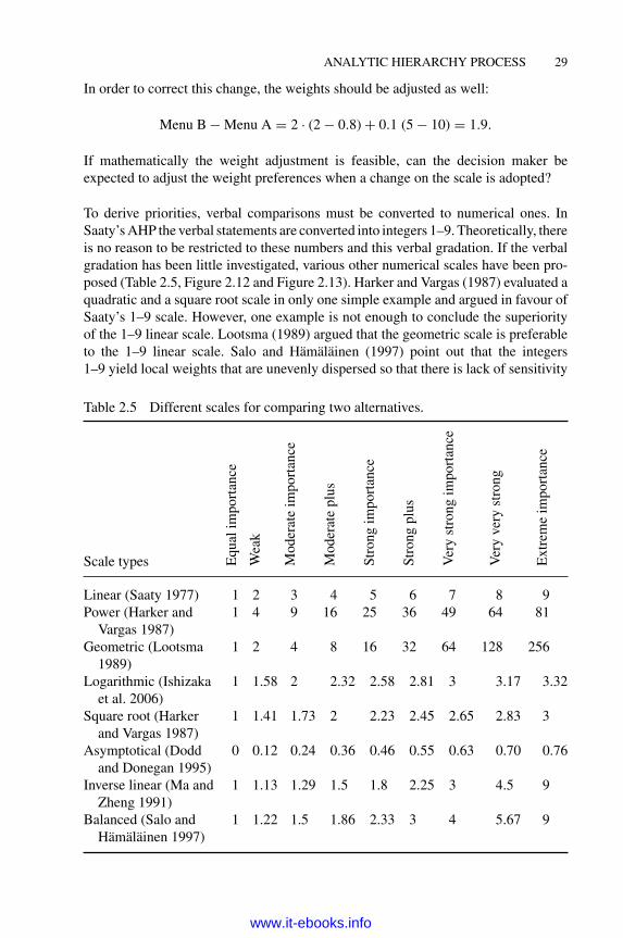
To derive priorities, verbal comparisons must be converted to numerical ones. InSaaty’s AHP the verbal statements are converted into integers 1–9. Theoretically, thereis no reason to be restricted to these numbers and this verbal gradation. If the verbalgradation has been little investigated, various other numerical scales have been pro-posed (Table 2.5, Figure 2.12 and Figure 2.13). Harker and Vargas (1987) evaluated aquadratic and a square root scale in only one simple example and argued in favour ofSaaty’s 1–9 scale. However, one example is not enough to conclude the superiorityof the 1–9 linear scale. Lootsma (1989) argued that the geometric scale is preferableto the 1–9 linear scale. Salo and Hamalainen (1997) point out that the integers1–9 yield local weights that are unevenly dispersed so that there is lack of sensitivity
Table 2.5 Different scales for comparing two alternatives.
Scale types Equ
alim
port
ance
Wea
k
Mod
erat
eim
port
ance
Mod
erat
epl
us
Stro
ngim
port
ance
Stro
ngpl
us
Ver
yst
rong
impo
rtan
ce
Ver
yve
ryst
rong
Ext
rem
eim
port
ance
Linear (Saaty 1977) 1 2 3 4 5 6 7 8 9Power (Harker and
Vargas 1987)1 4 9 16 25 36 49 64 81
Geometric (Lootsma1989)
1 2 4 8 16 32 64 128 256
Logarithmic (Ishizakaet al. 2006)
1 1.58 2 2.32 2.58 2.81 3 3.17 3.32
Square root (Harkerand Vargas 1987)
1 1.41 1.73 2 2.23 2.45 2.65 2.83 3
Asymptotical (Doddand Donegan 1995)
0 0.12 0.24 0.36 0.46 0.55 0.63 0.70 0.76
Inverse linear (Ma andZheng 1991)
1 1.13 1.29 1.5 1.8 2.25 3 4.5 9
Balanced (Salo andHamalainen 1997)
1 1.22 1.5 1.86 2.33 3 4 5.67 9
www.it-ebooks.info

30 MULTI-CRITERIA DECISION ANALYSIS
Figure 2.12 Graph of judgement scales.
when comparing elements which are preferentially close to each other. Based onthis observation, they propose a balanced scale where the local weights are evenlydispersed over the weight range [0.1, 0.9]. Earlier, Ma and Zheng (1991) calculateda scale where the inverse elements x of the scale 1/x are linear instead of the x inthe Saaty scale. Donegan et al. (1992) proposed an asymptotic scale avoiding theboundary problem (e.g. if the decision maker enters the pairwise comparison aij =3 and ajk = 4, they are forced into an intransitive relation because the upper limitof the scale is 9 and they cannot enter aik = 12). Ji and Jiang (2003) propose amixture of verbal scale and geometric scale. The possibility of integrating negativevalues into the scale has also been explored (Millet and Schoner 2005; Saaty andOzdemir 2003a).
Figure 2.13 Graph of the judgement scales with the geometric and power scalesomitted.
www.it-ebooks.info
ANALYTIC HIERARCHY PROCESS 31
Figure 2.12 and Figure 2.13 represent graphically the different scales of Table 2.5.Large differences are noted, which imply different final results (Ishizaka et al. 2010).
Among the proposed scales, the linear scale with the integers 1–9 and their recip-rocals have been used most often in applications. It is also the only one implementedin Expert Choice and MakeItRational. Saaty (1980, 1991) advocates it as the bestscale to represent weight ratios. However, the cited examples deal with objectivemeasurable alternatives like the areas of figures, whereas AHP treats mainly deci-sion processes on subjective issues. It is technically much more difficult to verifythe effectiveness of scales through subjective issues. Salo and Hamalainen (1997)demonstrate the superiority of the balanced scale when comparing two elements. Thechoice of the ‘best’ scale is a hotly debated issue. Some scientists argue that the choicedepends on the person and the decision problem (Harker and Vargas 1987; Poyhonenet al. 1997). Therefore, other scales would be welcomed in the AHP software.
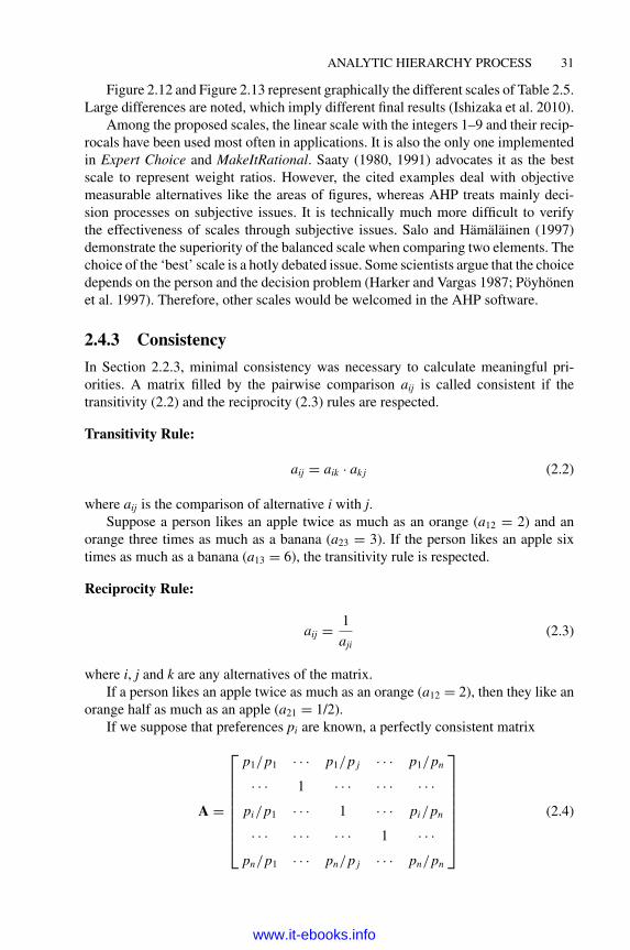
2.4.3 Consistency
In Section 2.2.3, minimal consistency was necessary to calculate meaningful pri-orities. A matrix filled by the pairwise comparison aij is called consistent if thetransitivity (2.2) and the reciprocity (2.3) rules are respected.
Transitivity Rule:
aij = aik · ak j (2.2)
where aij is the comparison of alternative i with j.Suppose a person likes an apple twice as much as an orange (a12 = 2) and an
orange three times as much as a banana (a23 = 3). If the person likes an apple sixtimes as much as a banana (a13 = 6), the transitivity rule is respected.
Reciprocity Rule:
aij = 1
aji(2.3)
where i, j and k are any alternatives of the matrix.If a person likes an apple twice as much as an orange (a12 = 2), then they like an
orange half as much as an apple (a21 = 1/2).If we suppose that preferences pi are known, a perfectly consistent matrix
A =
⎡⎢⎢⎢⎢⎢⎢⎢⎣
p1/p1 · · · p1/p j · · · p1/pn
· · · 1 · · · · · · · · ·pi/p1 · · · 1 · · · pi/pn
· · · · · · · · · 1 · · ·pn/p1 · · · pn/p j · · · pn/pn
⎤⎥⎥⎥⎥⎥⎥⎥⎦
(2.4)
www.it-ebooks.info

32 MULTI-CRITERIA DECISION ANALYSIS
can be constructed because all the comparisons aij obey the equality
aij = pi
p j, (2.5)
where pi is the priority of the alternative i.Priorities are not known in advance in AHP. As priorities only make sense if
derived from consistent or near-consistent matrices, a consistency check must beapplied. The threshold for defining an intolerably inconsistent matrix is not clear.Several methods have been proposed to measure consistency. Pelaez and Lamata(2003) describe a method based on the determinant of the matrix. Crawford andWilliams (1985) prefer to add the difference between the ratio of the calculatedpriorities and the given comparisons. The transitivity rule (2.2) was used by Salo andHamalainen (1997) and later by Ji and Jiang (2003). Stein and Mizzi (2007) use thenormalized column of the comparison matrix. However, the most commonly usedmethod (including in MakeItRational) was developed by Saaty (1977), who proposeda consistency index (CI), which is related to the eigenvalue method (Section 2.4.4):
CI = λmax − n
n − 1, (2.6)
where λmax is the maximal eigenvalue. The consistency ratio (CR) is given by
CR = CI/RI, (2.7)
where RI is the random index (the average CI of 500 randomly filled matrices). If CRis less than 10% (the inconsistency is less than 10% of 500 randomly filled matrices),then the matrix is of an acceptable consistency.
Saaty (1977) calculated the random indices shown in Table 2.6. Other researchershave run simulations with different numbers of matrices (Alonso and Lamata 2006;Lane and Verdini 1989; Tummala and Wan 1994) or incomplete matrices (Forman1990). Their random indices are different than but close to Saaty’s.
Alonso and Lamata (2006) have computed a regression of the random indicesand propose the formulation
λmax < n + 0.1(1.7699n − 4.3513). (2.8)
Table 2.6 Random indices from Saaty (1977).
n 3 4 5 6 7 8 9 10
RI 0.58 0.9 1.12 1.24 1.32 1.41 1.45 1.49
www.it-ebooks.info

ANALYTIC HIERARCHY PROCESS 33
For all proposed consistency checking methods, some questions remain: where isthe cut-off to declare the matrix inconsistent? Should this rule depend on the size ofthe matrix? How should the consistency definition be adapted when using anotherjudgement scale?
2.4.4 Priorities derivation
Priorities derivation is the corner-stone of the mathematics behind the AHP method,otherwise rankings could not be produced. Various methods have been proposed tocalculate priorities from a pairwise comparison matrix (Lin 2007; Cho and Wedley2004). In this section, three methods will be introduced: an approximate method, theeigenvalue method and the geometric mean. The approximate method requires onlyadditions and averages. The eigenvalue method calculates not only the priorities butalso the degree of inconsistency. The geometric mean has been proposed to solvethe problem of the right–left rank reversal of the eigenvalue method. Each methodcalculates identical priorities when matrices are consistent.
2.4.4.1 Approximate method
This method is based on two simple steps:
1. Summation of the elements of row i:
ri =∑
i
aij. (2.9)
2. Normalization of the sums:
pi = ri∑i ri
. (2.10)
Example 2.3 Suppose the decision maker has provided the comparisons inTable 2.7. The two steps are thus as follows:
1. The rows are summed as in the final column of Table 2.7.
2. Normalization the sums gives the criteria priorities as in Table 2.8
Table 2.7 Sum of the elements of the rows.
Industrial area Shopping centre City centre Total
Industrial area 1 6 2 9.00Shopping centre 1/6 1 1/2 1.67City centre 1/2 2 1 3.50
www.it-ebooks.info

34 MULTI-CRITERIA DECISION ANALYSIS
Table 2.8 Criteria priorities.
Industrial area Shopping centre City centre Total
Industrial area 1 6 2 0.64Shopping centre 1/6 1 1/2 0.12City centre 1/2 2 1 0.25
The approximate method does not calculate the consistency of the matrices.Therefore, all the AHP software packages that have been tested prefer to use a moreintensive calculation method, which allows the calculation of the inconsistency rate.
2.4.4.2 Eigenvalue method
In the eigenvalue method, the vector of the priorities p is calculated by solving theequation
Ap = np (2.11)
where n is the dimension of A and p = (p1, . . . , pj, . . . , pn).First, the validity of the eigenvalue method on a consistent matrix A is demon-
strated. Let us suppose that the priorities are known. It is easy to deduce a consistentcomparison matrix from the priorities as follows. Let aij = pi/p j . Multiplying A bythe priority vector p gives the right-hand side of equation (2.11). To simplify thecalculation, only row i of A is first considered:
pi
p1p1 + pi
p2p2 + . . . + pi
p jp j + . . . + pi
pnpn = pi + pi + . . . + pi + . . . + pi = npi
or
∑j
pi
p j· p j = npi . (2.12)
Thus the product of row i by the priority vector p gives n times the priority pi. Bymultiplying all the elements of the comparison matrix A by the priority vector p, thefollowing equality is obtained:
⎡⎢⎢⎢⎢⎣
p1/p1 p1/p2 · · · p1/pn
p2/p1 p2/p2 · · · p2/pn
· · · · · · · · · · · ·pn/p1 pn/p2 · · · pn/pn
⎤⎥⎥⎥⎥⎦
⎡⎢⎢⎢⎢⎣
p1
p2
· · ·pn
⎤⎥⎥⎥⎥⎦ = n
⎡⎢⎢⎢⎢⎣
p1
p2
· · ·pn
⎤⎥⎥⎥⎥⎦ ,
www.it-ebooks.info

ANALYTIC HIERARCHY PROCESS 35
Table 2.9 Consistent comparison matrix.
Industrial area Shopping centre City centre
Industrial area 1 6 3Shopping centre 1/6 1 1/2City centre 1/3 2 1
which is equation (2.11). Therefore, for a consistent matrix, the priority vector isobtained by solving equation (2.11).
Example 2.4 The eigenvalue problem is illustrated by the comparison matrix inTable 2.9. Because the comparison matrix is consistent, the priorities can be calculatedby solving (2.11):
Ap =
⎡⎢⎣
1 6 3
1/6 1 1/2
1/3 2 1
⎤⎥⎦ p = 3.p
The priority vector p is the solution of following the linear system:
1 · p1 + 6 · p2 + 3 · p3 = 3 · p1
1/6 · p1 + 1 · p2 + 1/2 · p3 = 3 · p1
1/6 · p1 + 1 · p2 + 1/2 · p3 = 3 · p1.
Solving this system for the unknowns p1, p2 and p3 results in
p =
⎡⎢⎣
p1
p2
p3
⎤⎥⎦ =
⎡⎢⎣
0.667
0.111
0.222
⎤⎥⎦ .
For an inconsistent matrix, this relation is no longer valid, as the comparisonbetween element i and j is not necessarily given by formula (2.5). Therefore, thedimension n is replaced by the unknown λ. The calculation of λ and p, from an equa-tion such as Ap = λp is called, in linear algebra, an eigenvalue problem. Any valueλ satisfying this equation is called an eigenvalue and p is its associated eigenvector.
According to the Perron theorem, a positive matrix has a unique positive eigen-value. The non-trivial eigenvalue is called the maximum eigenvalue λmax. If λmax =n, then the matrix is perfectly consistent. Otherwise, the difference between λmax – nis a measure of the inconsistency (Section 2.4.3).
www.it-ebooks.info

36 MULTI-CRITERIA DECISION ANALYSIS
Table 2.10 First iteration of the power method.
Industrial Shopping Sum of thearea centre City centre row Eigenvector
Industrial area 3 16 7 26 0.62Shopping centre 0.583 3 1.333 4.916 0.12City centre 1.333 7 3 11.333 0.27
42.249 1
Is the eigenvalue still valid for inconsistent matrices? Saaty (1977, 1980) justifiesthe eigenvalue approach for slightly inconsistent matrices with perturbation theory,which says that slight variations in a consistent matrix imply only slight variations ofthe eigenvector and eigenvalue.
In order to calculate the eigenvector associated to the maximum eigenvalue, mostsoftware packages, including MakeItRational, use the power method, which is aniterative process:
1. The pairwise matrix is squared: An+1 = AnAn.
2. The row sums are then calculated and normalized. This is the first approxima-tion of the eigenvector.
3. Using the matrix An+1, steps 1 and 2 are repeated.
4. Step 3 is repeated until the difference between these sums in two consecutivepriorities calculations is smaller than a given stop criterion.
Example 2.5 Considering the inconsistent matrix B of Table 2.7, the first iterationof the power method is given in Table 2.10.
The power method is not fully transparent, much less than the approximatemethod. Several articles have highlighted this irrationality. According to Johnsonet al. (1979), the ‘aggregation process embedded in the eigenvector . . . is not fullyunderstood mathematically’. Chu et al. (1979) say that ‘the weighted least squaresmethod . . . is conceptually easier to understand than the eigenvalue method’.
If the matrix of Table 2.11 is considered, it is known that a comparison can beestimated indirectly by the transitivity rule (2.2). Using (2.2), the comparison a13 iscalculated as follows:
a13 = a11 · a13 = 1 · 2 = 2,
a13 = a12 · a23 = 1/7 · 6 = 0.857,
a13 = a13 · a33 = 2 · 1 = 2,
a13 = a14 · a43 = 1/2 · 1 = 1/2.
www.it-ebooks.info

ANALYTIC HIERARCHY PROCESS 37
Table 2.11 Criteria comparison matrix with illustrative values.
Visibility Competition Frequency Rental cost
Visibility 1 1/7 2 1/2Competition 7 1 6 2Frequency 1/5 1/6 1 1Rental cost 2 1/2 1 1
It can be seen that the estimations of comparison a13 are very different. The matrixin Table 2.11 is thus inconsistent.
By squaring the matrix, the power method combines all the estimates of a13 dueto the scalar product of the first column and the third row of the matrix. In general,each element a′
ij of A2 is given by the sum a′ij = ∑
k aik · akj. Each additional squaringrefines the estimation of the comparison. Therefore, the eigenvalue method is basedon a procedure of averaging the direct and indirect estimations of the comparisons.
The eigenvalue method has a major drawback: the right–left inconsistency, whichleads to a rank reversal phenomenon after an inversion of the scale, was discoveredtwo years after the publication of the original AHP method (Johnson et al. 1979). Ifall comparisons are replaced by their reciprocal values (e.g., 5 becomes 1/5), then thederived ranking should logically also be reversed. This is not always the case for theeigen value method; however, if a matrix is perfectly consistent or of rank n = 3, thena rank reversal is impossible. For inconsistent matrices of rank n ≥ 4, rankings can bedifferent after a scale inversion. The following example illustrates this phenomenon.Consider the matrix in Table 2.12, asking ‘Which alternative is most economical?’.The calculated priorities give the following ranking of the alternatives: D > B > C >
A > E.If the question is inverted: ‘Which alternative is most expensive?’, then the
comparisons are simply inverted (Table 2.13). The calculated priorities give thefollowing ranking of the alternatives: B > D > C > A > E. In this case, alternative Bis preferred, but before it was alternative D. This rank reversal is due to the formulationof the problem (which is different from and independent of rank reversal due to theintroduction or deletion of an alternative, discussed in Section 2.4.5).
Table 2.12 Comparison matrix.
A B C D E Priority Rank
A 1 1/7 1/2 1/8 2 0.061 4B 7 1 3 1 8 0.374 2C 2 1/3 1 1/4 5 0.134 3D 8 1 4 1 5 0.387 1E 1/2 1/8 1/5 1/5 1 0.043 5
www.it-ebooks.info

38 MULTI-CRITERIA DECISION ANALYSIS
Table 2.13 Comparisons of Table 2.11 inverted.
A B C D E Priority Rank
A 1 7 2 8 1/2 0.299 4B 1/7 1 1/3 1 1/8 0.047 1C 1/2 3 1 4 1/5 0.140 3D 1/8 1 1/4 1 1/5 0.051 2E 2 8 5 5 1 0.462 5
2.4.4.3 Geometric mean
In order to avoid the left–right rank reversal, Crawford and Williams (1985) adoptedanother approach by minimizing the multiplicative error (2.13):
aij = pi
p jeij, (2.13)
where aij is the comparison between object i and j, pi is the priority of object I, andeij is the error.
The multiplicative error is commonly accepted to be log-normally distributed(similarly, the additive error would be assumed to be normally distributed). Thegeometric mean,
pi = n
√√√√ n∏j=1
aij, (2.14)
is the one, which minimizes the sum of these errors,
minn∑
i=1
n∑j=1
(1n(aij) − 1n
(pi
p j
))2
. (2.15)
The geometric mean (also sometimes known as logarithmic least squares method)can be easily calculated by hand and has been supported by a large segment of the AHPcommunity (Aguaron and Moreno-Jimenez 2000, 2003; Barzilai 1997; Barzilai andLootsma 1997; Budescu 1984; Escobar and Moreno-Jimenez 2000; Fichtner 1986;Leskinen and Kangas 2005; Lootsma 1993, 1996). Its main advantage is the absenceof rank reversals due to right–left inconsistency: the row and column geometric meansprovide the same ranking in an inverse order (this is not necessarily the case with theeigenvalue method).
www.it-ebooks.info

ANALYTIC HIERARCHY PROCESS 39
Example 2.6 The priorities of Table 2.12 are
p1 = 5
√1 · 1
7 · 12 · 1
8 · 2 = 0.447, p2 = 2.787,
p3 = .0.964, p4 = 2.759, p5 = 0.302.
Note that these priorities are in in the reverse order compared to the priorities ofTable 2.13: p1 = 2.237; p2 = 0.359; p3 = 1.037, p4 = 0.362, p5 = 3.314. Thereforethe geometric mean does not have any rank reversal due to an inversion of the scale.
2.4.5 Aggregation
The last necessary step is the synthesis of the local priorities across all criteria inorder to determine the global priority. The historical AHP approach adopts an additiveaggregation with normalization of the sum of the local priorities to unity. This type ofnormalization is called distributive mode. This additive aggregation is expressed as
Pi =∑
j
w j · pij (2.16)
where Pi is the global priority of alternative i, pij is the local priority with regard tocriterion j, and wj is the weight of the criterion j.
If priorities are known, the distributive mode is the only approach that willretrieve these priorities. However, if a copy (Belton and Gear 1983), or near-copy(the pairwise comparison is almost the same as the original) (Dyer 1990b), of analternative is introduced or removed (Troutt 1988), a rank reversal of the alternativesmay occur. This phenomenon has been criticized by some (Dyer 1990a, 1990b;Holder 1990, 1991; Stam and Duarte Silva 2003) and accepted by others (Harkerand Vargas 1987, 1990; Perez 1995; Saaty 1986, 1990, 1991, 1994b, 2006). Thisrank reversal phenomenon is not unique to AHP but common to all additive modelshaving a normalization step (Triantaphyllou 2001; Wang and Luo 2009). In fact,when the number of alternatives is changed, the denominator for the normalizationis also changed, which implies a change of scale and possible rank reversal.
To avoid this rank reversal problem, priorities should be normalized by dividingthem by the same denominator in any configuration of the problem for which theideal mode was proposed. This normalization is done by dividing the score of eachalternative by the score of the best alternative under each criterion.
When should the distributive or ideal mode be used? Millet and Saaty (2000) givesome guidance on which normalization to use. If in a closed system (i.e. no alternativewill be added or removed), then the distributive mode should be used. If in an opensystem (i.e. alternatives can be added or removed) and the preference is allowed foralternatives to be dependent on other alternatives (in other words, the rank reversalphenomenon is accepted), then the distributive mode is indicated. If we are in anopen system and do not want other alternatives to affect the outcome, then the idealmode is recommended.
www.it-ebooks.info

40 MULTI-CRITERIA DECISION ANALYSIS
Multiplicative aggregation has been proposed to prevent the rank reversal phe-nomenon observed in the distributive mode (Lootsma 1993; Barzilai and Lootsma1997). In the notation of (2.16), this form of aggregation is expressed as
pi =∏
j
pwj
ij (2.17)
Multiplicative aggregation has non-linear properties allowing a superior compro-mise to be selected; this is not the case with additive aggregation (Stam and DuarteSilva 2003; Ishizaka et al. 2006, 2010). Vargas (1997) demonstrated that additiveaggregation is the only way to retrieve exact weights of known objects. MakeItRa-tional offers only the additive distributive and ideal mode of aggregation.
Exercise 2.3
First you will learn to calculate priorities for one criterion step by step. Then you willbe given the opportunity to complete the spreadsheet for the other criteria.
Learning Outcomes
� Understand the calculation of priorities with the approximate method inMicrosoft Excel
� Understand the calculation of priorities with the eigenvalue method in Excel
� Understand the calculation of priorities with the geometric mean method inExcel
Tasks
Open the file Sport Shop.xls. It contains three spreadsheets with the three differentpriority calculation methods.
Complete the following tasks:
a) Describe the meaning of each calculation cell and its formula. Read thecomments in the red squares in case of difficulties.
b) The spreadsheets are incomplete because they calculate only one local alter-native. Complete them in order to calculate the other local alternatives.
2.5 Extensions of AHP
In this section, four extensions of AHP are presented. The analytic hierarchy pro-cess ordering method was introduced to separately analyse criteria that have to beminimized and maximized. The group analytic hierarchy process is used for groupdecisions. The clusters and pivots technique is applied to large problems to reduce thenumber of pairwise comparisons. AHPSort is implemented to solve sorting problems.
www.it-ebooks.info

ANALYTIC HIERARCHY PROCESS 41
Location of asports shop
Visibility Floor space
Industrial area Shopping centre City centre
Frequency Window size
Level 3
Level 2
Level 1
Figure 2.14 Benefit hierarchy.
2.5.1 Analytic hierarchy process ordering
The analytic hierarchy process ordering method, which considers incomparability,was first proposed by Ishizaka and Labib (2011). In line with the philosophy of AHP,some researchers have proposed deconstructing the model into sub-problems (Azis1990; Clayton et al. 1993; Wedley et al. 2001). They propose separating the criteriain opposite directions in different hierarchies: benefits versus cost. The reason forthis additional decomposition is that criteria in the same direction are much easier tocompare than in opposite directions, such as a criterion to be minimized and anothermaximized.
For example, suppose that three more criteria are added to Case Study 2.1:vandalism, floor space and window size. We now have seven criteria in total. Somehave to be maximized (visibility, floor space, frequency and window size) and othersminimized (competition, rental costs, vandalism). Two hierarchies can be constructed:a benefit hierarchy (Figure 2.14) and a cost hierarchy (Figure 2.15). These twohierarchies are then solved separately. As a result the output of the method is a partialranking (and not priorities).
Location of asports shop
Competition Rental costs
Industrial area Shopping centre City centre
Vandalism
Level 3
Level 2
Level 1
Figure 2.15 Cost hierarchy.
www.it-ebooks.info

42 MULTI-CRITERIA DECISION ANALYSIS
Benefit
Cost
0
0
Alternative AAlternative B
Figure 2.16 Graphical representation of the preference relation.
If cost and benefit rankings are not aggregated, we have a partial ordinal ranking(Ishizaka and Labib 2011). A partial ordinal ranking can be derived from the costand benefit analysis, where:
1. Alternative A is better than alternative B if alternative A is ranked better thanalternative B in the cost and benefit analysis (Figure 2.16).
2. Alternative A and alternative B are indifferent if alternative A has the samescore as alternative B in the cost and benefit analysis (Figure 2.17).
3. Alternative A is incomparable to alternative B if alternative A is better in oneanalysis and worse in the other analysis (Figure 2.18).
Incomparability does not exist in standard AHP. This status is important as it revealsthat a decision maker cannot decide which of the two alternatives is the best, whilenot being indifferent: an alternative is better in some aspects but worse in others. Todecide which alternative is better, further discussion between the decision makers andmoderation by the analyst are needed. This debate may require additional information.
However, if a debate cannot be held (e.g. if the decision maker is unavailable), thecost and benefit analysis can be merged into a complete ranking. First, the importancescores of the benefits and costs are weighted and then the weighted score of the costanalysis divides the weighted score of the benefit analysis. This produces the completecardinal ranking.
Benefit
Cost
0
0
Alternative AAlternative B
Figure 2.17 Graphical representation of the indifference relation.
www.it-ebooks.info

ANALYTIC HIERARCHY PROCESS 43
Benefit
Cost
0
0
Alternative AAlternative B
Figure 2.18 Graphical representation of incomparability.
Researchers have proposed four hierarchies: benefit, cost, opportunity and risk(Saaty and Ozdemir 2003a; Saaty 1994b). Each hierarchy is solved separately andthe local priorities are aggregated according to
pi = a · po + b · pb
c · pr + d · pc(2.18)
where a, b, c, d are weights, po is the priority of the opportunity hierarchy, pb is thepriority of the benefit hierarchy, pr is the priority of the risk hierarchy, and pc is thepriority of the cost hierarchy.
Exercise 2.4
In this exercise, you will be able to solve the sports shop problem with the AnalyticHierarchy Process Ordering.
Prerequisites
Exercise 2.2
Learning Outcomes
� Structure the benefit and cost hierarchy in MakeItRational
� Understand the partial ordinal ranking
� Understand the complete cardinal ranking
Tasks
a) In MakeItRational, construct the two hierarchies as in Figure 2.14 andFigure 2.15.
b) Evaluate the pairwise comparisons and calculate the priorities for eachhierarchy.
c) Draw a graph similar to that in Figure 2.16, Figure 2.17 or Figure 2.18.Confirm whether alternatives are preferred, indifferent or incomparable.
d) Aggregate the priorities of the two alternatives to obtain a complete cardinalranking.
www.it-ebooks.info

44 MULTI-CRITERIA DECISION ANALYSIS
Table 2.14 Four ways to combine preferences (Ishizaka and Labib 2011).
Mathematical aggregation
Yes No
Judgements(Figure 2.19)
Geometric mean oncomparisons
Consensus vote on comparisons
Priorities(Figure 2.20)
Weighted arithmetic meanon priorities
Consensus vote on priorities
Agg
rega
tion
on
2.5.2 Group analytic hierarchy process
2.5.2.1 Group aggregation
As a decision often affects several people, standard AHP has been adapted so thatit can be applied to group decisions. By consulting various experts, the bias oftenpresent when judgements are accepted from a single expert is eliminated. There arefour ways to combine the preferences into a consensus rating (Table 2.14).
The consensus vote is used when there is a synergistic group and not a collectionof individuals. In this case, the hierarchy of the problem must be the same for alldecision makers. On the judgement level, this method requires the group to reachan agreement on the value of each entry in a matrix of pairwise comparisons. Aconsistent agreement is usually difficult to obtain, the difficulty increasing with thenumber of comparison matrices and related discussions. To bypass this difficulty, theconsensus vote can be postponed until after the calculation of the priorities for eachparticipant. O’Leary (1993) recommends this version because an early aggregationcould result ‘in a meaningless average performance measure’. An aggregation afterthe calculation of priorities allows decision makers with different opinions to bedetected and further discussion over any disagreement.
If a consensus cannot be reached (e.g. with a large number of people or peoplein different locations), a mathematical aggregation can be adopted. Two synthesizingmethods exist and provide the same results in the case of perfect consistency in thepairwise matrices (Saaty and Vargas 2005). In the first method, the geometric meanof the individual evaluations is used as an element in the pairwise matrices and thenpriorities are calculated from that (Figure 2.19). The geometric mean method must beadopted instead of the arithmetical mean to preserve the reciprocal property (Aczeland Saaty 1983). For example, if person A enters comparison 9 and person B enters
1/9, then by intuition the mathematical consensus should be√
9 · 19 = 1, which is a
geometric mean and not (9 + 1/9)/2 = 4.56, which is an arithmetic mean. However,Ramanathan and Ganesh (1994) give an example where the Pareto optimality (i.e.if all group members prefer A to B, then the group decision should prefer A) is notsatisfied with the geometric mean method. Van den Honert and Lootsma (1997) argue
www.it-ebooks.info

ANALYTIC HIERARCHY PROCESS 45
Person 1
Person 2
Person n
Comparisons ofperson 1
Comparisons ofperson 2
Comparisons ofperson n
Aggregation ofcomparisons
Calculation ofpriorities
Figure 2.19 Aggregation at the comparison level.
that this violation is expected because the pairwise assessments are a compromiseof all the group members’ assessments and, therefore, the compromise does notrepresent any one opinion of the group members. Madu and Kuei (1995) and Saatyand Vargas (2007) introduce a measure of the dispersion of the judgements to avoidthis problem. If the group is not homogeneous, further discussions are required toreach a consensus.
In the second method (Figure 2.20), decision makers constitute the first levelbelow the goal of the AHP hierarchy (Figure 2.21). Priorities are computed and thenaggregated using the weighted arithmetic mean method. Applications can be found inLabib and Shah (2001) and Labib et al. (1996). Arbel and Orgler (1990) introduceda level above that of the stakeholders representing the several economic scenarios.This extra level determines the priorities (weights) of the stakeholders.
In a compromise method an individual’s derived priorities can be aggregated ateach node. According to Forman and Peniwati (1998), this method is ‘less meaningfuland not commonly used’. Aggregation methods with linear programming (Mikhailov2004) and the Bayesian approach (Altuzarra et al. 2007) have been proposed to makea decision even when comparisons are missing, for example, when a stakeholder doesnot have the expertise to judge a particular comparison.
A group decision may be skewed due to collusion or distortion in the judgementsto secure the preferred outcome. This problem does not arise when there is a singledecision maker because the first choice will always remain the first. In a groupdecision, a participant does not have this certitude as the results are aggregated withthose of the other stakeholders. One decision maker may overweight their preferredalternative and bias the group decision. As individual identities are lost with anaggregation, early aggregation is not recommended.
www.it-ebooks.info

46 MULTI-CRITERIA DECISION ANALYSIS
Person 1
Person 2
Person n
Comparisons ofperson 1
Comparisons ofperson 2
Comparisons ofperson n
Aggregation ofpriorites
Calculation ofpriorities person 1
Calculation ofpriorities person 2
Calculation ofpriorities person n
Figure 2.20 Aggregation at the priorities level.
2.5.2.2 Weight of stakeholders
If the decision makers do not have equal weight, their priorities must be determinedas discussed in Ishizaka and Labib (2011). The weights should reflect the expertiseof a decision maker (Weiss and Rao 1987) or the importance of the impact of the
Location of asports shop
Visibility Competition
Industrial area Shopping centre City centre
Frequency Rental cost
Level 4
Level 3
Level 1
Stakeholder A Stakeholder B Stakeholder CLevel 2
Figure 2.21 Hierarchy including the stakeholders.
www.it-ebooks.info
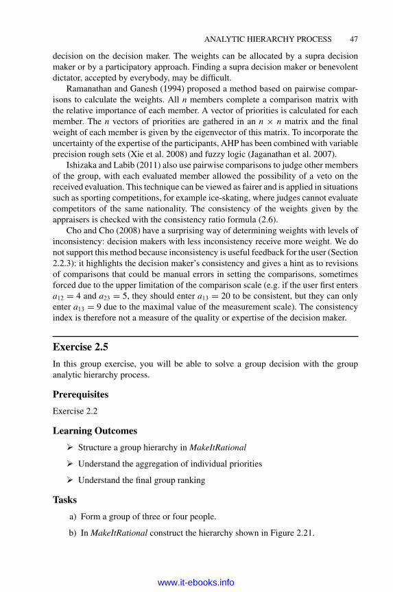
ANALYTIC HIERARCHY PROCESS 47
decision on the decision maker. The weights can be allocated by a supra decisionmaker or by a participatory approach. Finding a supra decision maker or benevolentdictator, accepted by everybody, may be difficult.
Ramanathan and Ganesh (1994) proposed a method based on pairwise compar-isons to calculate the weights. All n members complete a comparison matrix withthe relative importance of each member. A vector of priorities is calculated for eachmember. The n vectors of priorities are gathered in an n × n matrix and the finalweight of each member is given by the eigenvector of this matrix. To incorporate theuncertainty of the expertise of the participants, AHP has been combined with variableprecision rough sets (Xie et al. 2008) and fuzzy logic (Jaganathan et al. 2007).
Ishizaka and Labib (2011) also use pairwise comparisons to judge other membersof the group, with each evaluated member allowed the possibility of a veto on thereceived evaluation. This technique can be viewed as fairer and is applied in situationssuch as sporting competitions, for example ice-skating, where judges cannot evaluatecompetitors of the same nationality. The consistency of the weights given by theappraisers is checked with the consistency ratio formula (2.6).
Cho and Cho (2008) have a surprising way of determining weights with levels ofinconsistency: decision makers with less inconsistency receive more weight. We donot support this method because inconsistency is useful feedback for the user (Section2.2.3): it highlights the decision maker’s consistency and gives a hint as to revisionsof comparisons that could be manual errors in setting the comparisons, sometimesforced due to the upper limitation of the comparison scale (e.g. if the user first entersa12 = 4 and a23 = 5, they should enter a13 = 20 to be consistent, but they can onlyenter a13 = 9 due to the maximal value of the measurement scale). The consistencyindex is therefore not a measure of the quality or expertise of the decision maker.
Exercise 2.5
In this group exercise, you will be able to solve a group decision with the groupanalytic hierarchy process.
Prerequisites
Exercise 2.2
Learning Outcomes
� Structure a group hierarchy in MakeItRational
� Understand the aggregation of individual priorities
� Understand the final group ranking
Tasks
a) Form a group of three or four people.
b) In MakeItRational construct the hierarchy shown in Figure 2.21.
www.it-ebooks.info
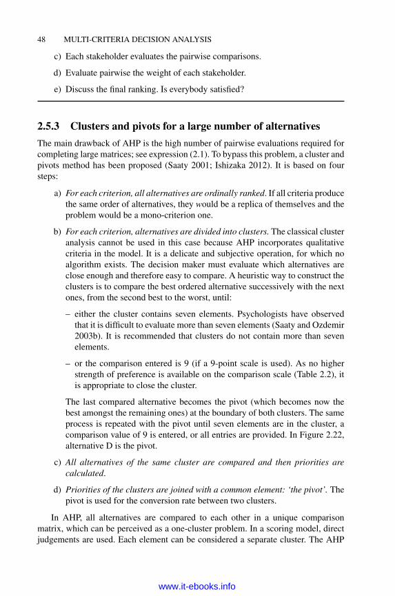
48 MULTI-CRITERIA DECISION ANALYSIS
c) Each stakeholder evaluates the pairwise comparisons.
d) Evaluate pairwise the weight of each stakeholder.
e) Discuss the final ranking. Is everybody satisfied?
2.5.3 Clusters and pivots for a large number of alternatives
The main drawback of AHP is the high number of pairwise evaluations required forcompleting large matrices; see expression (2.1). To bypass this problem, a cluster andpivots method has been proposed (Saaty 2001; Ishizaka 2012). It is based on foursteps:
a) For each criterion, all alternatives are ordinally ranked. If all criteria producethe same order of alternatives, they would be a replica of themselves and theproblem would be a mono-criterion one.
b) For each criterion, alternatives are divided into clusters. The classical clusteranalysis cannot be used in this case because AHP incorporates qualitativecriteria in the model. It is a delicate and subjective operation, for which noalgorithm exists. The decision maker must evaluate which alternatives areclose enough and therefore easy to compare. A heuristic way to construct theclusters is to compare the best ordered alternative successively with the nextones, from the second best to the worst, until:
– either the cluster contains seven elements. Psychologists have observedthat it is difficult to evaluate more than seven elements (Saaty and Ozdemir2003b). It is recommended that clusters do not contain more than sevenelements.
– or the comparison entered is 9 (if a 9-point scale is used). As no higherstrength of preference is available on the comparison scale (Table 2.2), itis appropriate to close the cluster.
The last compared alternative becomes the pivot (which becomes now thebest amongst the remaining ones) at the boundary of both clusters. The sameprocess is repeated with the pivot until seven elements are in the cluster, acomparison value of 9 is entered, or all entries are provided. In Figure 2.22,alternative D is the pivot.
c) All alternatives of the same cluster are compared and then priorities arecalculated.
d) Priorities of the clusters are joined with a common element: ‘the pivot’. Thepivot is used for the conversion rate between two clusters.
In AHP, all alternatives are compared to each other in a unique comparisonmatrix, which can be perceived as a one-cluster problem. In a scoring model, directjudgements are used. Each element can be considered a separate cluster. The AHP
www.it-ebooks.info

ANALYTIC HIERARCHY PROCESS 49
A B C D E FA 1 9B 1C 1D 1E 1F 1
Figure 2.22 Building clusters.
and scoring model represent the two extremes, where 1 or n clusters are used. Thismodel is the middle way between the two methods.
Example 2.7 Suppose that in Case Study 2.1, the businessman has to choose whereto situate the sports shop from a choice of 12 cities. In this example, only one criterionis considered (e.g. quality of life), as the process is identical with several criteria.
a) Alternatives are preordered. The 12 cities are preordered according to theirquality of life: A, B, C, D, E, F, G, H, I, J, K, L.
b) Alternatives are divided into clusters. The best city for quality of life, A, iscompared successively with the next cities until the comparison entered is9 (Table 2.15). As city A is 9 times better than F for its quality, alternative Fis declared the pivot: the last element in the first cluster and the first elementin the second cluster.
c) Comparisons are entered in clustered matrices and priorities are calculated.Notice that the process requires 30 comparisons (highlighted in grey in
Table 2.15 Comparison matrix for the criterion quality – the unnecessarycomparisons are shaded grey.
A B C D E F G H I J K L
A 1 2 3 5 8 9B 1 2 3 6 7C 1 3 5 6D 1 4 5E 1 2F 1 1 3 4 5 5 7G 1 3 3 4 5 7H 1 2 3 4 6I 1 2 2 4J 1 1 3K 1 3L 1
www.it-ebooks.info

50 MULTI-CRITERIA DECISION ANALYSIS
Table 2.16 First cluster of cities.
Cities Priority
F 0.311G 0.289H 0.157I 0.097J 0.061K 0.057L 0.028
Table 2.17 Second cluster of cities.
Cities PrioritiesPriorities linked
with the first cluster
A 0.404 4.333B 0.249 2.670C 0.178 1.909D 0.101 1.083E 0.040 0.429F 0.029 0.311
Table 2.15) less than the classical AHP approach. Priorities are calculatedfor both clusters (Tables 2.16 and 2.17).
d) Priorities of both clusters are joined with a common element: ‘the pivot’.Results of the second cluster (Table 2.17) are linked to the first (Table 2.16)by dividing them by the ratio of the scores of pivot F in the two clusters:0.311/0.029. Final results are given in Table 2.18.
2.5.4 AHPSort
Whilst AHP solves ranking problems, AHPSort has been developed for sorting prob-lems (Ishizaka et al. 2012). This method is a variant of AHP used when alternativeshave to be sorted into categories predefined with central limiting profiles. Supposethat the businessman in Case Study 2.1 aims to open several sports shops in differentcities. The cities will be sorted into three classes (Figure 2.23):
a) cities where sports shops will be highly profitable;
b) cities where sports shop may be profitable;
c) cities where sports shops will not be profitable.
www.it-ebooks.info

ANALYTIC HIERARCHY PROCESS 51
Table 2.18 Priorities of the cities.
Cities Priorities
A 4.333B 2.670C 1.909D 1.083E 0.429F 0.311G 0.289H 0.157I 0.097J 0.061K 0.057L 0.028
AHPSort is based on eight steps:
A) Problem definition
1) Define the goal, criteria and alternatives of the problem.
2) Define the categories Ci, i = 1, . . . , n.
3) Define the profiles of each class. This can be done with limiting profileslpi, which indicate the minimum performance needed on each criterion tobelong to class Ci, or with central profiles cpi, given by a typical exampleof an element belonging to class Ci. To define each class, n – 1 limitingprofiles or n central profiles are needed.
B) Evaluations
4) Evaluate pairwise the importance of the criteria and derive weights(Section 2.4.4).
Class 1:Set of retained cities
Class 3:Set of discarded cities
AHPSortAlternatives
Limiting profile for class 1
Limiting profile for class 2
Class 2:Set of possible
cities
Figure 2.23 AHPSort for the sorting process.
www.it-ebooks.info

52 MULTI-CRITERIA DECISION ANALYSIS
Class 1
Class 2
Class 3
Class 4
Class 5
Class 6
lp1
lp2
lp3
lp4
lp5
pjmust be greater
than lpi to belong toclass Ci
Figure 2.24 Sorting with limiting profiles.
5) Compare in a pairwise comparison matrix a single candidate to be sortedwith limiting or central profiles for each criterion to derive local prioritiesfor each criterion (Section 2.4.4).
6) Aggregate the local weighted priorities, which provide a global prioritypj of alternative aj.
C) Assignment to classes
7) The global priority pj is used to assign the alternative aj to class Ci.
a) Limiting profiles. If limiting profiles have been defined, then alternativeaj is assigned to class Ci which has the lpi just below the global prioritypj (Figure 2.24).
p j ≥ lp1 ⇒ a j ∈ C1
lp2 ≤ p j < lp1 ⇒ a j ∈ C2
· · ·p j < lpn−1 ⇒ a j ∈ Cn
b) Central profiles. Alternative aj is assigned to class Ci which has thenearest central profile cpi to pj (Figure 2.25). In the case of equaldistance between two central profiles, the optimistic assignment vision
www.it-ebooks.info

ANALYTIC HIERARCHY PROCESS 53
Class 1
Class 2
Class 3
Class 4
Class 5
Class 6
cp1
cp2
cp3
cp4
cp5
pjis assigned to
class Ci, which hasthe closest cpi
cp6
Figure 2.25 Sorting with central profiles.
allocates aj to the upper class, whilst the pessimistic assignment visionallocates aj to the lower class.
pi ≥ cp1 ⇒ a j ∈ C1
cp2 ≤ p j < cp1 AND (cp1 − p j ) < (cp2 − p j ) ⇒ a j ∈ C1
cp2 ≤ p j < cp1 AND (cp1 − p j ) = (cp2 − p j ) ⇒ a j ∈ C1 in the
optimistic vision
cp2 ≤ p j < cp1 AND (cp1 − p j ) = (cp2 − p j ) ⇒ a j ∈ C2 in the
pessimistic vision
cp2 ≤ p j < cp1 AND (cp1 − p j )>(cp2 − p j ) ⇒ a j ∈ C2
· · ·p j < cpn ⇒ a j ∈ Cn (2.19)
8) Repeat steps 4–7 for each alternative to be classified.
Exercise 2.6
In this exercise, you will sort cities into three categories:
a) cities where sports shops must be open;
b) cities where sports shops may be opened later;
c) cities where sports shops would not be profitable.
www.it-ebooks.info

54 MULTI-CRITERIA DECISION ANALYSIS
Prerequisites
Exercise 2.2
Learning Outcomes
� Structure a sorting problem in MakeItRational
� Define classes
� Understand the sorting results
Tasks
a) Choose 10 potential cities as alternatives for opening a sports shop.
b) Define two limiting profiles for each class.
c) Model the problem in MakeItRational.
d) Enter the pariwise comparison for each city.
e) Sort the city into a category according to its score.
References
Aczel, J., and Saaty, T. (1983). Procedures for synthesizing ratio judgements. Journal ofMathematical Psychology, 27(1), 93–102.
Aguaron, J., and Moreno-Jimenez, J. (2000). Local stability intervals in the analytic hierarchyprocess. European Journal of Operational Research, 125(1), 113–132.
Aguaron, J., and Moreno-Jimenez, J. (2003). The geometric consistency index: Approximatedthresholds. European Journal of Operational Research, 147(1), 137–145.
Alonso, J., and Lamata, T. (2006). Consistency in the analytic hierarchy process: A newapproach. International Journal of Uncertainty, Fuzziness and Knowledge-Based Systems,14(4), 445–459.
Altuzarra, A., Moreno-Jimenez, J., and Salvador, M. (2007). A Bayesian priorization proce-dure for AHP-group decision making. European Journal of Operational Research, 182(1),367–382.
Arbel, A., and Orgler, Y. (1990). An application of the AHP to bank strategic planning: Themergers and acquisitions process. European Journal of Operational Research, 48(1), 27–37.
Azis, I. (1990). Analytic hierarchy process in the benefit-cost framework: A post-evaluationof the Trans-Sumatra highway project. European Journal of Operational Research, 48(1),38–48.
Barzilai, J. (1997). Deriving weights from pairwise comparisons matrices. Journal of theOperational Research Society, 48(12), 1226–1232.
Barzilai, J. (2005). Measurement and preference function modelling. International Transac-tions in Operational Research, 12(2), 173–183.
Barzilai, J., and Lootsma, F. (1997). Power relation and group aggregation in the multiplicativeAHP and SMART. Journal of Multi-Criteria Decision Analysis, 6(3), 155–165.
www.it-ebooks.info

ANALYTIC HIERARCHY PROCESS 55
Belton, V., and Gear, A. (1983). On a shortcoming of Saaty’s method of analytical hierarchies.Omega, 11(3), 228–230.
Budescu, D. (1984). Scaling binary comparison matrices: A comment on Narasimhan’s pro-posal and other methods. Fuzzy Sets and Systems, 14(2), 187–192.
Cho, E., and Wedley, W. (2004). A common framework for deriving preference values frompairwise comparison matrices. Computers and Operations Research, 31(6), 893–908.
Cho, Y.-G., and Cho, K.-T. (2008). A loss function approach to group preference aggregationin the AHP. Computers & Operations Research, 35(3), 884–892.
Chu, A., Kalabra, R., and Spingarn, K. (1979). A comparison of two methods for determiningthe weights of belonging to fuzzy sets. Journal of Optimization Theory and Applications,27(4), 531–538.
Clayton, W., Wright, M., and Sarver, W. (1993). Benefit cost analysis of riverboat gambling.Mathematical and Computer Modelling, 17(4–5), 187–194.
Crawford, G., and Williams, C. (1985). A note on the analysis of subjective judgementmatrices. Journal of Mathematical Psychology, 29(4), 387–405.
Dodd, F., and Donegan, H. (1995). Comparison of priotization techniques using interhierarchymappings. Journal of the Operational Research Society, 46(4), 492–498.
Donegan, H., Dodd, F., and McMaster, T. (1992). A new approach to AHP decision-making.The Statician, 41(3), 295–302.
Dyer, J. (1990a). A clarification of ‘Remarks on the analytic hierarchy process’. ManagementScience, 36(3), 274–275.
Dyer, J. (1990b). Remarks on the analytic hierarchy process. Management Science, 36(3),249–258.
Escobar, M., and Moreno-Jimenez, J. (2000). Reciprocal distributions in the analytic hierarchyprocess. European Journal of Operational Research, 123(1), 154–174.
Fichtner, J. (1986). On deriving priority vectors from matrices of pairwise comparisons. Socio-Economic Planning Sciences, 20(6), 341–345.
Forman, E. (1990). Random indices for incomplete pairwise comparison matrices. EuropeanJournal of Operational Research, 48(1), 153–155.
Forman, E., and Peniwati, K. (1998). Aggregating individual judgements and prioritieswith the analytic hierarchy process. European Journal of Operational Research, 108(1),165–169.
Harker, P., and Vargas, L. (1987). The theory of ratio scale estimation: Saaty’s analytichierarchy process. Management Science, 33(11), 1383–1403.
Harker, P., and Vargas, L. (1990). Reply to ‘Remarks on the analytic hierarchy process’.Management Science 36(3), 269–273.
Holder, R. (1990). Some comment on the analytic hierarchy process. Journal of the OperationalResearch Society, 41(11), 1073–1076.
Holder, R. (1991). Response to Holder’s comments on the analytic hierarchy process: Responseto the response. Journal of the Operational Research Society, 42(10), 914–918.
Ishizaka, A. (2012). A multicriteria approach with AHP and clusters for the selection amonga large number of suppliers. Pesquisa Operacional, 32(1), 1–15.
Ishizaka, A., Balkenborg, D., and Kaplan, T. (2006). Influence of aggregation and preferencescale on ranking a compromise alternative in AHP. Paper presented at the MultidisciplinaryWorkshop on Advances in Preference Handling.
www.it-ebooks.info

56 MULTI-CRITERIA DECISION ANALYSIS
Ishizaka, A., Balkenborg, D., and Kaplan, T. (2010). Influence of aggregation and mea-surement scale on ranking a compromise alternative in AHP. Journal of the OperationalResearch Society, 62(4), 700–710.
Ishizaka, A., and Labib, A. (2009). Analytic hierarchy process and Expert Choice: benefitsand limitations. OR Insight, 22(4), 201–220.
Ishizaka, A., and Labib, A. (2011). Selection of new production facilities with the groupanalytic hierarchy process ordering method. Expert Systems with Applications, 38(6), 7317–7325.
Ishizaka, A., Nemery, P., and Pearman, C. (2012). AHPSort: An AHP based method forsorting problems. International Journal of Production Research, 50(17), 4767–4784.
Jaganathan, S., Erinjeri, J., and Ker, J. (2007). Fuzzy analytic hierarchy process basedgroup decision support system to select and evaluate new manufacturing technologies.International Journal of Advanced Manufacturing Technology, 32(11), 1253–1262.
Ji, P., and Jiang, R. (2003). Scale transitivity in the AHP. Journal of the Operational ResearchSociety, 54(8), 896–905.
Johnson, C., Beine, W., and Wang, T. (1979). Right-left asymmetry in an eigenvector rankingprocedure. Journal of Mathematical Psychology, 19(1), 61–64.
Kainulainen, T., Leskinen, P., Korhonen, P., Haara, A., and Hujala, T. (2009). A statisticalapproach to assessing interval scale preferences in discrete choice problems. Journal of theOperational Research Society, 60(2), 252–258.
Kaspar, R., Ossadnik, W. (2013) Evaluation of AHP software from a management accountingperspective. Journal of Modelling in Management, 8(3), in press.
Labib, A., and Shah, J. (2001). Management decisions for a continuous improvement pro-cess in industry using the analytical hierarchy process. Journal of Work Study, 50(5),189–193.
Labib, A., Williams, G., and O’Connor, R. (1996). Formulation of an appropriate productivemaintenance strategy using multiple criteria decision making. Maintenance Journal, 11(11),66–75.
Lane, E., and Verdini, W. (1989). A consistency test for AHP decision makers. DecisionSciences, 20(3), 575–590.
Leskinen, P., and Kangas, J. (2005). Rank reversal in multi-criteria decision analysis with sta-tistical modelling of ratio-scale pairwise comparisons. Journal of the Operational ResearchSociety, 56(7), 855–861.
Lin, C. (2007). A revised framework for deriving preference values from pairwise comparisonmatrices. European Journal of Operational Research, 176(2), 1145–1150.
Lootsma, F. (1989). Conflict resolution via pairwise comparison of concessions. EuropeanJournal of Operational Research, 40(1), 109–116.
Lootsma, F. (1993). Scale sensitivity in the multiplicative AHP and SMART. Journal of Multi-Criteria Decision Analysis, 2(2), 87–110.
Lootsma, F. (1996). A model for the relative importance of the criteria in the multiplicativeAHP and SMART. European Journal of Operational Research 94(3), 467–476.
Ma, D., and Zheng, X. (1991). 9/9-9/1 scale method of AHP. Paper presented at the 2ndInternational Symposium on AHP.
Madu, C., and Kuei, C.-H. (1995). Stability analyses of group decision making. Computers &Industrial Engineering, 28(4), 881–892.
www.it-ebooks.info

ANALYTIC HIERARCHY PROCESS 57
Mikhailov, L. (2004). Group prioritization in the AHP by fuzzy preference programmingmethod. Computers & Operations Research, 31(2), 293–301.
Millet, I., and Saaty, T. (2000). On the relativity of relative measures: Accommodating bothrank preservation and rank reversals in the AHP. European Journal of Operational Research,121(1), 205–212.
Millet, I., and Schoner, B. (2005). Incorporating negative values into the analytic hierarchyprocess. Computers and Operations Research 32(12), 3163–3173.
O’Leary, D. (1993). Determining differences in expert judgement: Implications for knowledgeacquisition and validation. Decision Sciences, 24(2), 395–408.
Pelaez, P., and Lamata, M. (2003). A new measure of consistency for positive reciprocalmatrices. Computers & Mathematics with Applications, 46(12), 1839–1845.
Perez, J. (1995). Some comments on Saaty’s AHP. Management Science, 41(6), 1091–1095.
Poyhonen, M., Hamalainen, R., and Salo, A. (1997). An experiment on the numericalmodelling of verbal ratio statements. Journal of Multi-Criteria Decision Analysis, 6(1),1–10.
Ramanathan, R., and Ganesh, L. (1994). Group preference aggregation methods employed inAHP: An evaluation and an intrinsic process for deriving members’ weightages. EuropeanJournal of Operational Research, 79(2), 249–265.
Saaty, T. (1977). A scaling method for priorities in hierarchical structures. Journal of Mathe-matical Psychology, 15(3), 234–281.
Saaty, T. (1980). The Analytic Hierarchy Process. New York: McGraw-Hill.
Saaty, T. (1986). Axiomatic foundation of the analytic hierarchy process. Management Science,32(7), 841–855.
Saaty, T. (1990). An exposition of the AHP in reply to the paper ‘Remarks on the analytichierarchy process’. Management Science, 36(3), 259–268.
Saaty, T. (1991). Response to Holder’s comments on the analytic hierarchy process. Journalof the Operational Research Society, 42(10), 909–929.
Saaty, T. (1994a). Highlights and critical points in the theory and application of the analytichierarchy process. European Journal of Operational Research 74(3), 426–447.
Saaty, T. L. (1994b). Fundamentals of Decision Making and Priority Theory. Pittsburgh: RWSPublications.
Saaty, T. (2001). The seven pillars of the analytic hierarchy process. Paper presented atthe Multiple Criteria Decision Making in the New Millennium. Proceedings of the 15thInternatinal Conference MCDM, Istanbul.
Saaty, T. (2006). Rank from Comparisons and from ratings in the analytic hierarchy/networkprocesses. European Journal of Operational Research, 168(2), 557–570.
Saaty, T., and Forman, E. (1992). The Hierarchon: A Dictionary of Hierarchies (Vol. V).Pittsburgh: RWS Publications.
Saaty, T., and Ozdemir, M. (2003a). Negative priorities in the analytic hierarchy process.Mathematical and Computer Modelling, 37(9–10), 1063–1075.
Saaty, T., and Ozdemir, M. (2003b). Why the magic number seven plus or minus two. Math-ematical and Computer Modelling, 38(3–4), 233–244.
Saaty, T. L., and Vargas, L. G. (2005). The possibility of group welfare functions. InternationalJournal of Information Technology & Decision Making, 4(2), 167–176.
www.it-ebooks.info

58 MULTI-CRITERIA DECISION ANALYSIS
Saaty, T., and Vargas, L. (2007). Dispersion of group judgements. Mathematical and ComputerModelling, 46(7–8), 918–925.
Salo, A., and Hamalainen, R. (1997). On the measurement of preference in the analytichierarchy process. Journal of Multi-Criteria Decision Analysis, 6(6), 309–319.
Stam, A., and Duarte Silva, P. (2003). On multiplicative priority rating methods for AHP.European Journal of Operational Research, 145(1), 92–108.
Stein, W., and Mizzi, P. (2007). The harmonic consistency index for the analytic hierarchyprocess. European Journal of Operational Research, 177(1), 488–497.
Stillwell, W., von Winterfeldt, D., and John, R. (1987). Comparing hierarchical and non-hierarchical weighting methods for eliciting multiattribute value models. ManagementScience, 33(4), 442–450.
Thurstone, L. (1927). A law of comparative judgements. Psychological Review, 34(4), 273–286.
Triantaphyllou, E. (2001). Two new cases of rank reversals when the AHP and some of itsadditive variants are used that do not occur with the multiplicative AHP. Journal of Multi-Criteria Decision Analysis, 10(1), 11–25.
Troutt, M. (1988). Rank reversal and the dependence of priorities on the underlying mavfunction. Omega,16(4), 365–367.
Tummala, V., and Wan, Y. (1994). On the mean random inconsistency index of the analytichierarchy process (AHP). Computers & Industrial Engineering 27(1–4), 401–404.
Van Den Honert, R., and Lootsma, F. (1997). Group preference aggregation in the multiplica-tive AHP The model of the group decision process and Pareto optimality. European Journalof Operational Research, 96(2), 363–370.
Vargas, L. (1997). Comments on Barzilai and Lootsma: Why the multiplicative AHP is invalid:A practical counterexample. Journal of Multi-Criteria Decision Analysis, 6(4), 169–170.
Wang, Y., and Luo, Y. (2009). On rank reversal in decision analysis. Mathematical andComputer Modelling, 49(5–6), 1221–1229.
Weber, M., Eisenfuhr, F., and von Winterfeldt, D. (1988). The effects of spitting attributes onweights in multiattribute utility measurement. Management Science, 34(4), 431–445.
Wedley, W., Choo, E., and Schoner, B. (2001). Magnitude adjustment for AHP benefit/costratios. European Journal of Operational Research, 133(2), 342–351.
Weiss, E., and Rao, V. (1987). AHP design issues for large-scale systems. Decision Sciences,18(1), 43–57.
Xie, G., Zhang, J., Lai, K., and Yu, L. (2008). Variable precision rough set for groupdecision-making: An application. International Journal of Approximate Reasoning, 49(2),331–343.
Yokoyama, M. (1921). The nature of the affective judgement in the method of paired compar-ison. American Journal of Psychology, 32, 357–369.
www.it-ebooks.info

3
Analytic network process
3.1 Introduction
This chapter explains the theory and practical uses of the analytic network processmethod (ANP). You will learn how to use Super Decisions (Section 3.3), a softwarepackage that helps to structure decision problems and calculate priorities (scores)based on the ANP methodology. As ANP is a generalization of the analytic hierar-chy process (AHP), it is advisable to read Chapter 2 first in order to ensure betterunderstanding. Section 3.4 is dedicated to the methodological background of ANP.The companion website provides illustrative examples withMicrosoft Excel, and
case studies and an example with Super Decisions.
3.2 Essential concepts of ANP
ANP is a generalization of AHP which deals with dependencies. In AHP, as with theother methods presented in this book, we assume that criteria are independent. If theyare not independent, correlated criteria would result in an overevaluated weight inthe decision, as will be illustrated. For example, if we want to buy a car, the criteriaof speed and engine power are correlated. In the traditional MCDA methods, thisdependency implies a heavier weight of these joint criteria. The ANP method allowsthese dependencies, also called feedbacks, to be modelled; they are closer to realityand, as a result, yield more accurate results. As dependencies can arise between anyof the elements in the decision problem (i.e. alternatives, criteria, sub-criteria, thegoal), the model is no longer linear as in AHP (Figure 3.1), where the elements arearranged in levels. A hierarchy is not necessary in the ANP model, where clustersreplace the levels and each cluster contains nodes or elements (see Figure 3.2). Theclusters are connected by a line, which in turn means that the elements or nodescontained are connected.
Multi-Criteria Decision Analysis: Methods and Software, First Edition. Alessio Ishizaka and Philippe Nemery.© 2013 John Wiley & Sons, Ltd. Published 2013 by John Wiley & Sons, Ltd.
www.it-ebooks.info
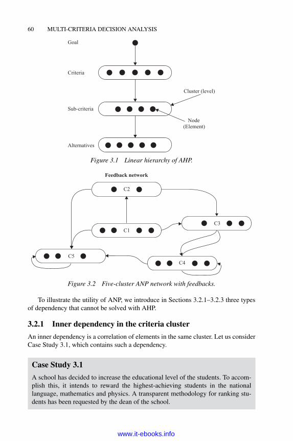
60 MULTI-CRITERIA DECISION ANALYSIS
Goal
Criteria
Sub-criteria
Alternatives
Cluster (level)
Node(Element)
Figure 3.1 Linear hierarchy of AHP.
C2
C5
C3C1
C4
Feedback network
Figure 3.2 Five-cluster ANP network with feedbacks.
To illustrate the utility of ANP, we introduce in Sections 3.2.1–3.2.3 three typesof dependency that cannot be solved with AHP.
3.2.1 Inner dependency in the criteria cluster
An inner dependency is a correlation of elements in the same cluster. Let us considerCase Study 3.1, which contains such a dependency.
Case Study 3.1
A school has decided to increase the educational level of the students. To accom-plish this, it intends to reward the highest-achieving students in the nationallanguage, mathematics and physics. A transparent methodology for ranking stu-dents has been requested by the dean of the school.
www.it-ebooks.info

ANALYTIC NETWORK PROCESS 61
The structure of Case Study 3.1 has three levels: goal, criteria and alternatives.The evaluation is biased towards the scientific students, as there is a high
correlation between the mathematics and physics courses. This inner dependencein the cluster cannot be modelled with AHP.As an illustrative case, we consider two students: Shakespeare and Newton.
Shakespeare has a talent for languages and Newton excels in scientific subjects.If the criteria are assumed to have the same weight, the result calculated by AHPwould favour Newton as his strengths lie in the two scientific criteria (see Figure3.3). ANP is necessary for modelling the inner dependency.
Figure 3.3 Evaluation of Shakespeare and Newton with AHP inMakeItRational.Reproduced by permission of BS Consulting Dawid Opydo.
The ANP problem structure is very similar to that of AHP, with three levels ofclusters: goal, criteria and alternatives. The difference is the additional loop over thecluster criteria, which indicates an inner dependency (Figure 3.4).In addition to the pairwise comparisons in traditional AHP,matricesmodelling the
inner dependency are required. These matrices aim to capture the relative importance
Best Student
Maths Physics Language
Shakespeare Newton
Goal
Criteria
Alternatives
Figure 3.4 Case Study 3.1 structured in clusters.
www.it-ebooks.info

62 MULTI-CRITERIA DECISION ANALYSIS
of the criteria when another dependent criterion has already been evaluated. In CaseStudy 3.1, three additional matrices are required. The questions to be answered areas follows:
� If your goal is to select the best student and you know that you are evaluatingthem against Physics, which other criterion, Language or Maths, would bemore important and by how much?As there is a strong correlation between Maths and Physics, a stronger
importance (9 times more important) is given to Language.
� If your goal is to select the best student and you know that you are evaluatingthem against Language, which other criterion, Maths or Physics, would bemore important and by how much?As there is neither a correlation between Language and Physics, nor
between Language and Maths, a similar weight is given to both criteria.
� If your goal is to select the best student and you know that you are evaluatingthem against Maths, which other criterion, Language or Physics, would bemore important and by how much?As there is strong correlation betweenMaths and Physics, a stronger impor-
tance (9 times more important) is given to Language.
The results are different than those calculated using AHP (Figure 3.5). TheLanguage criterion receives a much higher weight (0.47) than the two other criteria(0.26). Newton (0.52) and Shakespeare (0.48) are now very close in their ranking,giving an unbiased evaluation.If the decision maker set a weight of 0.5 for Language and 0.25 for Maths and
Physics, the comparison to enter would be an infinite amount more important toLanguage compared to Maths and Physics. This is technically impossible to enter inthe software but can be approximated with a very high number.
Figure 3.5 Ranking with ANP. C© 1999/2003 Thomas L. Saaty. Reproduced bypermission of Thomas L. Saaty.
www.it-ebooks.info
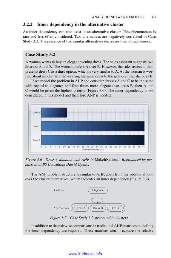
ANALYTIC NETWORK PROCESS 63
3.2.2 Inner dependency in the alternative cluster
An inner dependency can also exist in an alternative cluster. This phenomenon israre and less often considered. Two alternatives are negatively correlated in CaseStudy 3.2. The presence of two similar alternatives decreases their attractiveness.
Case Study 3.2
A woman wants to buy an elegant evening dress. The sales assistant suggests twodresses: A and B. The woman prefers A over B. However, the sales assistant thenpresents dress C as a third option, which is very similar to A. As the woman is wor-ried about another woman wearing the same dress to the gala evening, she buys B.If we model the problem in AHP and consider dresses A and C to be the same
with regard to elegance and four times more elegant than dress B, then A andC would be given the highest priority (Figure 3.6). The inner dependency is notconsidered in this model and therefore ANP is needed.
Figure 3.6 Dress evaluation with AHP in MakeItRational. Reproduced by per-mission of BS Consulting Dawid Opydo.
The ANP problem structure is similar to AHP, apart from the additional loopover the cluster alternatives, which indicates an inner dependency (Figure 3.7).
Elegance
Dress A Dress B Dress C
Criteria
Alternatives
Figure 3.7 Case Study 3.2 structured in clusters.
In addition to the pairwise comparisons in traditional AHP, matrices modellingthe inner dependency are required. These matrices aim to capture the relative
www.it-ebooks.info

64 MULTI-CRITERIA DECISION ANALYSIS
importance of the alternatives, when it is known that another dependent alternativehas already been evaluated. In Case Study 3.2, three new matrices modelling theinner dependency are required. The questions to be answered are as follows:
� If your goal is to select your preferred dress and you know that dress A isalso in the evaluation cluster, which dress, B or C, is preferred?As dresses A and C are similar, dress B will be preferred (9 times more
important).
� If your goal is to select your preferred dress and you know that dress B isalso in the evaluation cluster, which dress, A or C, is preferred?As dresses A and C are similar and there is no correlation with dress B,
they are equally preferred.
� If your goal is to select your preferred dress and you know that dress C isalso in the evaluation cluster, which dress, A or B, is preferred?As dresses A and C are similar, dress B is preferred (9 times more
important).
The global priorities are now different than in AHP (Figure 3.5). Dress B isthe preferred alternative (Figure 3.8).
Figure 3.8 Dress ranking with ANP. C© 1999/2003 Thomas L. Saaty. Reproducedby permission of Thomas L. Saaty.
3.2.3 Outer dependency
An outer dependency or feedback is a correlation between two clusters. For example,we can have an outer dependency between the cluster criteria and the cluster alter-native: the weight of the criteria depends on the available alternatives. In AHP, thesefeedbacks can be captured through intuitive iterations. For example, in Case Study3.3, the woman changes the weight of the criteria once she has learnt the price of the
www.it-ebooks.info
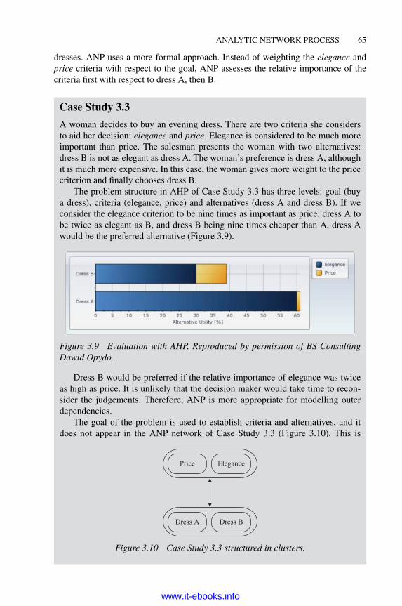
ANALYTIC NETWORK PROCESS 65
dresses. ANP uses a more formal approach. Instead of weighting the elegance andprice criteria with respect to the goal, ANP assesses the relative importance of thecriteria first with respect to dress A, then B.
Case Study 3.3
A woman decides to buy an evening dress. There are two criteria she considersto aid her decision: elegance and price. Elegance is considered to be much moreimportant than price. The salesman presents the woman with two alternatives:dress B is not as elegant as dress A. The woman’s preference is dress A, althoughit is much more expensive. In this case, the woman gives more weight to the pricecriterion and finally chooses dress B.The problem structure in AHP of Case Study 3.3 has three levels: goal (buy
a dress), criteria (elegance, price) and alternatives (dress A and dress B). If weconsider the elegance criterion to be nine times as important as price, dress A tobe twice as elegant as B, and dress B being nine times cheaper than A, dress Awould be the preferred alternative (Figure 3.9).
Figure 3.9 Evaluation with AHP. Reproduced by permission of BS ConsultingDawid Opydo.
Dress B would be preferred if the relative importance of elegance was twiceas high as price. It is unlikely that the decision maker would take time to recon-sider the judgements. Therefore, ANP is more appropriate for modelling outerdependencies.The goal of the problem is used to establish criteria and alternatives, and it
does not appear in the ANP network of Case Study 3.3 (Figure 3.10). This is
Price Elegance
Dress A Dress B
Figure 3.10 Case Study 3.3 structured in clusters.
www.it-ebooks.info

66 MULTI-CRITERIA DECISION ANALYSIS
conceptually surprising, especially for a decision maker using other MCDAmeth-ods. The justification for this absence is that no element in the problem dependson the goal: in this case, the weight of the criteria depends on the alternativesavailable and not on the goal.As a result, in Figure 3.10, there is an arrow with double direction. If the
weight of the criteria does not depend on the available alternatives, a goal needs tobe added and the arrow between the criteria cluster and alternatives cluster wouldpoint in the direction of the alternatives.In addition to the pairwise comparisons asked in traditional AHP, matrices
modelling the outer dependency are required. These matrices aim to capture therelative importance of the criteria, with regard to the alternatives. In Case Study 3.3two additional matrices (one for each alternative) are required.The questions to answer are:
� If your goal is to buy a dress, and you know that dress B is in the cluster ofthe alternatives, which criterion, elegance or price, is more important andby how much?As dress B is elegant and moderately expensive, an extreme importance
(9 times as much) is given to elegance.
� If your goal is to buy a dress, and you know that dress A is in the cluster ofthe alternatives, which criterion, elegance or price, is more important andby how much?As dress A is elegant but also expensive, a moderate amount of impor-
tance (3 times as much) is given to price.
The results are now different than those in AHP (Figure 3.11). The elegancecriterion is given a more moderate weight and, as a result, dress B is preferred.
Figure 3.11 Dress ranking with ANP. C© 1999/2003 Thomas L. Saaty. Repro-duced by permission of Thomas L. Saaty.
www.it-ebooks.info

ANALYTIC NETWORK PROCESS 67
Table 3.1 Influence matrix for a simple hierarchy.
Goal Alternatives Criteria
A1 A2 A3 A4 C2 C3 C4
Goal
A1 x x xA2 x x xA3 x x xA4 x x xA
lternatives
C1 xC2 xC3 xC
riteria
3.2.4 Influence matrix
When the problem has been formulated and criteria and alternatives defined, it isgood practice to complete an influence matrix. The influence matrix records with across any dependency between elements of the network. In AHP, the influence matrixwould look like Table 3.1: the evaluation of the criteria depends on the goal, andthe evaluation of the alternative depends on the criteria. In ANP, additional Xs inthe influence matrix are possible to indicate the dependences between the differentelements. If the criteria depend on the alternatives, the cluster goal is removed fromthe influence matrix (see Section 3.2.3).
Exercise 3.1
The following multiple-choice questions allow you to test your basic knowledgeof ANP. Only one answer is correct. Answers can be found on the companionwebsite.
1. What does ANP stand for?
a) Analytic Neural Program
b) Analytic Neural Process
c) Analytic Network Process
d) Analytical Network Program
www.it-ebooks.info

68 MULTI-CRITERIA DECISION ANALYSIS
2. What is an inner dependency?
a) A correlation between two clusters
b) A correlation between decision makers
c) A correlation between alternatives and criteria
d) A correlation of nodes in the same cluster
3. What is ‘feedback’ in an ANP structure?
a) A correlation between two clusters
b) A sensitivity analysis
c) An inner dependency
d) A master–slave dependency
4. Which of the following statements is false?
a) ANP is more precise than AHP
b) ANP requires more pairwise comparisons than AHP
c) ANP is an extension of AHP
d) ANP, unlike AHP, uses direct evaluations
5. In ANP, a goal node is not necessary when . . .
a) Criteria depend on alternatives
b) Alternatives depends on criteria
c) A goal is unclear
d) There is an inner dependency
3.3 ANP software: Super Decisions
There are two main programs that support ANP: Super Decisions andDecision Lens.Super Decisions has been developed for teaching purposes and can be downloaded,free of charge, from http://www.superdecisions.com. Decision Lens is an expensivecommercial software package used in industry. Due to the cost of this software, ithas not been possible to test it, so no comment can be made. In this section, theessentials for using Super Decisions are provided. A full tutorial can be downloadedfrom http://www.superdecisions.com/demos_tutorials.php3.When using Super Decisions it is not necessary to understand how priorities are
calculated. The decision maker identifies what should be ranked and the correlationsbetween the elements in the problem.
www.it-ebooks.info

ANALYTIC NETWORK PROCESS 69
To illustrate Super Decisions, the example of the purchase of an evening dress,as described in Case Study 3.4, will be used throughout this section.
Case Study 3.4
A woman would like to buy one of three evening dresses:
Salsaly.1 a) Red lace ruffle dress in silk. Bodycon fit and one shoulder. Laceruffle from shoulder to centre front and from back centre. The dress is awell-known Italian brand (same as the Tangal dress) designed by a famousGerman designer. It is priced at £2700.
Tangal. b) Asymmetric red draped dress in silk. Draped detail to front and back,with flower embellishment on shoulder. The dress is a well-known Italianbrand (same as the Salsaly dress) designed by a famous French designer. Itis priced at £2000.
Xenthila. c) Black minidress in satin. A wrap over chiffon drape design, withcontrast mesh top, plunging V neck and sleeveless styling. The dress is aFrench brand by a famous Italian designer. It is priced at £1900.
The decision will be based on four criteria (Table 3.2).
Table 3.2 Criteria for dress purchase.
Criteria Explanation
Brand Brand usually determines prestige and qualityDesigner Designer is related to prestige and creativityFabric Fabric of the dressPrice Price of the dress
3.3.1 Problem structuring
Before using the software, it is important to structure the problem. All the elements(nodes) should be listed. These usually result frombrainstorming and are then groupedinto clusters.In Super Decisions, new clusters can be created by selecting Design/Cluster/New
from the menu. Similarly, new alternatives are added by selecting Design/Node/New.The next step is to detect the influence one node could have on the others. Once
detected, there are two ways to create links between the parent and child nodes.
1The names of the dresses are fictitious. Any resemblance to existing names is entirely coincidental.
www.it-ebooks.info

70 MULTI-CRITERIA DECISION ANALYSIS
� From themenu selectDesign/Node connexions from. From the list that appears,select a parent (or source) node. A second list will appear for all dependentnodes to be selected.
� Click on the ‘three arrows’ icon Do connexions. Left-click on the source nodeand right-click on all the dependent nodes, which will turn red.There are three types of dependencies:
� Outer dependencies:
� Criteria influence the choice of an alternative with regard to the purchaseof an evening dress, therefore all cells on the upper right-hand side of thematrix will always contain Xs.
� The available alternatives influence the weight of the criteria, therefore allcells on the lower left-hand side of the matrix contain Xs.
� Inner dependencies cluster criteria:
� The brand has a renowned name, which influences the price.
� The name of the designer influences the price of the dress, as well as thetype of the fabric used.
� The fabric influences the price of the dress.
� Inner dependencies cluster alternatives:The availability of one alternative may have an influence on another. Forexample, a woman may decide not buy a dress if a similar one is available, asit might be awkward to see another woman wearing an almost identical dresson the same night (see Case Study 3.2).
There is no obligation to compile an influence matrix; the influence mapping canbe done directly on the network diagram (e.g. Figure 3.12). However, an influencediagram like Table 3.3 gives a global view and a common reference for a groupdiscussion. The nodes are grouped in clusters: criteria and alternatives. The goalnode does not exist because in this case, the weight of the criteria depends on thealternatives available and not the goal. If the weight of the criteria does not dependon the available alternatives, a goal needs to be added.
3.3.2 Assessment of pairwise comparison
All the nodes to be pairwise compared are always in the same cluster. They arecompared with respect to their parent node and provide local priorities. In order tostart the process, you need to selectAssess/Compare thenNode Comparisons from themenu and click on Do Comparison. Four comparison modes are available: graphic,verbal, matrix and questionnaire. Figure 3.13 displays the questionnaire mode wherethe Salsaly and Tangal dresses are equivalent with regard to brand preference; theSalsaly brand is 5 times as preferable as that of Xenthila and Tangal is 5 times as
www.it-ebooks.info

ANALYTIC NETWORK PROCESS 71
Figure 3.12 Case Study 3.4 structured with Super Decisions. C© 1999/2003 ThomasL. Saaty. Reproduced by permission of Thomas L. Saaty.
preferable as Xenthila. To switch from one mode to another, you need to click on thetop buttons.To calculate the priorities and inconsistencies from any of the comparison modes,
select Computations/Show new Priorities. In Figure 3.14 the local priorities of thematrix shown in Figure 3.13 are displayed. Salsaly and Tangal are the two most
Table 3.3 Influence matrix of Case Study 3.4.
Alternatives Criteria
Salsaly Tangal Xenthila Brand Designer Fabric Price
Salsaly x x x x x xTangal x x x x x xXenthila x x x x x x
Alternatives
Brand x x x xDesigner x x x x xFabric x x x xPrice x x xCriteria
www.it-ebooks.info

72 MULTI-CRITERIA DECISION ANALYSIS
Figure 3.13 Pairwise comparisons of alternatives in Super Decisions. C© 1999/2003Thomas L. Saaty. Reproduced by permission of Thomas L. Saaty.
preferred alternatives with regard to brand. The matrix is consistent because theinconsistency index is 0. If the inconsistency index is higher than 0.1, it is advisableto revise the comparisons. To do this, select Computation/Most inconsistent fromthe menu where the most inconsistent comparison will be shown. For example, inFigure 3.15, themost inconsistent comparison, 2, is highlighted. The best replacementvalue is calculated by clicking Show Best Value.
Super Decisions allows a direct rating of the alternatives/criteria if they are alreadyknown. For example, in Figure 3.16, the price of each dress is known, therefore anexact amount can be entered. As a higher price is less preferable, the priorities needto be inverted, which is done by checking Inverted. If all evaluation preferences arerated directly, then a weighted sum is being used. Super Decisions supports ANP,AHP and a weighted sum because they share various common features.
Figure 3.14 Local priorities in Super Decisions. C© 1999/2003 Thomas L. Saaty.Reproduced by permission of Thomas L. Saaty.
www.it-ebooks.info

ANALYTIC NETWORK PROCESS 73
Figure 3.15 Most inconsistent comparison is highlighted. C© 1999/2003 Thomas L.Saaty. Reproduced by permission of Thomas L. Saaty.
3.3.3 Results
The global priorities of the alternatives are obtained by selecting Computations/Synthesize from the menu or by clicking on the icon (Figure 3.12). TheIdeals column is obtained from the Normals column by dividing each priority bythe largest value, which means that the best alternative always has a score of 1. TheNormals column normalizes the priorities to 1 and the Raw column comes fromthe limit supermatrix (see Section 3.4). In Figure 3.17, the Xenthila dress would bethe better option.
Figure 3.16 Direct rating of the alternatives. C© 1999/2003 Thomas L. Saaty. Repro-duced by permission of Thomas L. Saaty.
www.it-ebooks.info

74 MULTI-CRITERIA DECISION ANALYSIS
Figure 3.17 Global priorities in Super Decisions. C© 1999/2003 Thomas L. Saaty.Reproduced by permission of Thomas L. Saaty.
3.3.4 Sensitivity analysis
The sensitivity analysis in ANP is more complicated than in AHP. In AHP, onecriterion weight can be changed, whereas in ANP, each node can be linked to anothernode; an independent nodemust be definedwith regard to a parent node. The followingsteps are used in Super Decisions:
� Select Computations/Sensitivity from the menu to access the sensitivitymodule.
� Select Edit/Independent Variable from the menu.
� In the Edit parameter window, select SuperMatrix for the Parameter Type, theparent node (Wrt Node, i.e. With respect to) and the independent node (1stother node). For example, in Figure 3.18, the independent variable is Priceand the parent node is Salsaly.
� Click on Done on the Edit parameter window.
� Click on Update on the Sensitivity input selector.
In Figure 3.19, the weight of Price is plotted on the x-axis and the priorities ofthe alternatives are plotted on the y-axis. By clicking and dragging the black dottedvertical line it is possible to change the local priority of Price. We can appreciate thatin any scenario, the Xenthila dress is a robust choice.
www.it-ebooks.info

ANALYTIC NETWORK PROCESS 75
Figure 3.18 Parent and independent nodes. C© 1999/2003 Thomas L. Saaty. Repro-duced by permission of Thomas L. Saaty.
Figure 3.19 Sensitivity analysis in Super Decisions. C© 1999/2003 Thomas L. Saaty.Reproduced by permission of Thomas L. Saaty.
www.it-ebooks.info

76 MULTI-CRITERIA DECISION ANALYSIS
Exercise 3.2
In this exercise, you will solve the evening dress problem set out in Case Study 3.4with the Super Decisions software.
Learning Outcomess
� Structure a problem in Super Decisions
� Enter pairwise comparisons
� Understand the results
� Conduct a sensitivity analysis
Tasks
a) Open the Super Decisions software.
b) Read the description of Case Study 3.4 on page 69.
c) Enter the clusters (Design/Cluster/New).
d) Enter the nodes (Design/Node/New).
e) Link the dependent nodes (Design/Node connexions from).
f) Enter the pairwise comparisons (Menu Assess/compare then Cluster Com-parisons). Are they consistent?
g) Read your global ranking (Computations/Synthesize).
h) Conduct a sensitivity analysis (Computations/Sensitivity).
3.4 In the black box of ANP
ANP rests on the same theory as AHP (Section 2.4), the only difference being thesupermatrix. In this section, the priorities calculation from the supermatrix will beexplained. The supermatrix is a partitionedmatrix, where each submatrix is composedof a set of relationships between two nodes in the network. It is similar to Table 3.3,but consists of intensities instead of Xs. The priority calculation is based on theMarkov chains process, which is explained in the following section.
3.4.1 Markov chain
A Markov chain, named after Andrey Markov, is a system that undergoes randomtransitions from one state to another with no memory of the past. This means thatonly the current state of the process can influence the next state. A more extensivepresentation can be found in Norris (1997). As a simple example, we consider fourchildren (Tom, Sam, Liz and Franz) passing a ball to each other. As they have different
www.it-ebooks.info

ANALYTIC NETWORK PROCESS 77
Tom Sam Liz Franz
Tom 0 0.2 0.5 0.3
Sam 0.4 0 0.4
Liz 0.4 0.3 0 0.3
Franz 0.1 0.3 0.6 0
0.2
Figure 3.20 Transition probability matrix.
Tom Sam Liz Franz
Tom 0.31 0.24 0.22 0.23
Sam 0.12 0.26 0.44 0.18
Liz 0.15 0.17 0.44 0.24
Franz 0.36 0.20 0.11 0.33
Figure 3.21 Probability matrix after the second transition.
affinities, the ball is passed with unequal probabilities among them. The matrix inFigure 3.20 contains the transition probability of the ball from one child to another.For example, the probability of Tom giving the ball to Sam is 0.2, to Liz 0.5, and toFranz 0.3. The section across the diagonal will always be zero as the child will notkeep the ball at each transition but pass it to another child. It is important to note thatthe sum of each row is 1, which indicates that the ball is always with a child. Theprobabilities are unchanged during the game because a previous pass has no influenceon the next one.In order to find the ball after the second transition, the matrix is squared
(Figure 3.21).If the number of transitions is infinite (i.e. high), the probabilities will stabilize
and be identical in each column (Figure 3.22). This indicates that at the end of thegame. After a large number of transitions, the probability of the ball being with Tomis 0.233, with Sam is 0.213, with Liz is 0.307 and with Franz is 0.247.
Tom Sam Liz Franz
Tom 0.232755 0.212865 0.307237 0.247143
Sam 0.232755 0.212865 0.307237 0.247143
Liz 0.232755 0.212865 0.307237 0.247143
Franz 0.232755 0.212865 0.307237 0.247143
Figure 3.22 Probability matrix after a large number of transitions.
www.it-ebooks.info

78 MULTI-CRITERIA DECISION ANALYSIS
Exercise 3.3
You will cover the Markov chain process step by step.
Learning Outcomes
� Understand how a probability matrix is compiled
� Understand the calculation of probabilities
Tasks
Open the file Ball Game.xls. It contains a spreadsheet with the calculation ofpriorities from a supermatrix.Answer the following questions:
a) Describe the meaning of each cell in the supermatrix. (Read the comments inthe red box in case of difficulty.)
b) Calculate by hand the second probability matrix.
3.4.2 Supermatrix
The influence of each node on other nodes in a network can be gathered in a superma-trix (Saaty, 2001). The supermatrix in Figure 3.23 sets out the influence on the threeclusters: goal, alternatives and criteria. The order of these in the matrix is irrelevant(this is not the case with the hierarchy in AHP). If dependencies do not exist between
Goal Alternatives CriteriaCluster nodemodel
A1 A2 A3 C1 C2 C3
Goal 0 0 0 0 0 0 0
A1 0
A2 0Alternatives
A3 0
eigenvector of influence on eachalternative (because of inner dependency
in the alternative cluster)
local priority ofalternative Ai with regard
to criteria Ci
C1 0 0 0
C2 0 0 0
C3 0 0 0Criteria
Weightof the
criteria
eigenvector of influenceon each criterion(because of inner
dependency in thecriteria cluster)
Figure 3.23 Supermatrix with no outer dependency from the alternatives of thecriteria.
www.it-ebooks.info

ANALYTIC NETWORK PROCESS 79
Alternatives CriteriaCluster node
modelA1 A2 A3
A1
Alternatives A2
eigenvector of influence on eachalternative (because of inner dependency
in the alternative cluster)
local priority ofalternative Ai with regard
to criteria Ci
A3
C1
C2
C3
Criteria
weight of the criteria with regard to eachalternative
eigenvector of influenceon each criterion(because of inner
dependency in thecriteria cluster)
C1 C2 C3
Figure 3.24 Supermatrix with outer dependency from the alternatives on the criteria.
nodes, zero is entered. For example, only the grey sections in Figure 3.23 are com-pleted. The network becomes a hierarchy and, as a result, AHP can be used; howeverthe calculation can still be done using ANP. The results are the same in both cases.However, the disadvantage is that the calculation is more time-consuming. AHP usesa simple weighted sum for aggregation, whereas ANP requires the supermatrix to besquared many times. Because of this, ANP is not recommended if no dependencyexists.If an outer dependency from the alternatives on the criteria exists, the cluster goal
can be removed and the weights with regard to each alternative can be added (sectionshown in grey on Figure 3.24).The columns in the supermatrixmust be normalized to 1 in order to have a stochas-
tic matrix that can be used in a Markov chain process. To capture the transmission ofinfluence along all possible paths of the network, the matrix is raised to powers. Thematrix is squared to represent the direct influence of one element on another. Thecubic power is taken to express the indirect influence of a second element, and so on.As the matrix is stochastic, it will converge to a limit supermatrix, which containsthe global priorities.
Exercise 3.4
You will learn to calculate priorities from a supermatrix step by step.
Learning Outcomes
� Understand how a supermatrix is completed
� Understand the calculation of priorities from the supermatrix
www.it-ebooks.info
80 MULTI-CRITERIA DECISION ANALYSIS
Tasks
Open the file Evening Dress.xls. It contains a spreadsheet with the calculation ofpriorities from a supermatrix.Answer the following questions:
a) Why does each column in the matrix have to be normalized to 1?
b) Describe the meaning of each cell in the supermatrix. (Read the comments inthe red box in case of difficulty.)
References
Norris, J. (1997).Markov Chains. Cambridge: Cambridge University Press.
Saaty, T. (2001). The Analytic Network Process. Pittsburgh: RWS Publications.
www.it-ebooks.info

4
Multi-attribute utility theory
4.1 Introduction
This chapter explains the theory and practical uses of themulti-attribute ultility theory(MAUT) method. You will learn how to use RightChoice, a software package thathelps to structure decision problems and calculate scores based on theMAUTmethod.Section 4.3 is designed for readers interested in the methodological backgroundof MAUT. As the MAUT method requires the decision maker to specify lots ofinput parameters, some ‘elicitation’ methods are presented in Section 4.4. The UTA,UTAGMS and GRIP elicitation methods help to infer preference parameters froma sample ranking given by the decision maker. This section will include a briefdescription of the UTA+ and VisualUTA software.The companion website provides illustrative examples withMicrosoft Excel, and
case studies and an example with RightChoice.
4.2 Essential concepts of MAUT
MAUT is widely used in the Anglo-Saxon world and is based on the main hypothesisthat every decisionmaker tries to optimize, consciously or implicitly, a functionwhichaggregates all their points of view. This means that the decision maker’s preferencescan be represented by a function, called the utility function U (Keeney and Raiffa1976). This function is not necessarily known at the beginning of the decision process,so the decision maker needs to construct it first.The utility function is a way of measuring the desirability or the preference of
objects, called alternatives. These can be consumer goods (cars, smartphones, etc.)or services. The utility score is the degree of well-being those alternatives provide
Multi-Criteria Decision Analysis: Methods and Software, First Edition. Alessio Ishizaka and Philippe Nemery.© 2013 John Wiley & Sons, Ltd. Published 2013 by John Wiley & Sons, Ltd.
www.it-ebooks.info

82 MULTI-CRITERIA DECISION ANALYSIS
A
d
c
a
b
U(f1(a), ... ,fq(a))
1
0
U(.)
U(d )
U(a)=U(b)
U(c)...
Figure 4.1 Representation of the ranking of the set A using the MAUT model.
to the decision maker. The utility function is composed of various criteria whichenable the assessment of the global utility of an alternative. Consider, for instance,the purchase of a smartphone (see Case Study 4.1). In order to choose the mostappropriate smartphone, one will measure the global utility of those available. Theutility is usually grounded on several criteria, such as price, customer reviews, size.For each criterion, the decision maker will give a score, called the marginal utilityscore. The marginal utility scores of the criteria will be aggregated in a second phaseto the global utility score.Each alternative of set A is evaluated on the basis of function U and receives
a ‘utility score’ U (a) (see Figure 4.1). This utility score allows the ranking of allalternatives from best to worst. The preference and indifference relations amongstthe alternatives of A are thus defined as follows:
∀ a, b ∈ A : a P b ⇔ U (a) > U (b) : a is preferred to b, (4.1)
∀ a, b ∈ A : a I b ⇔ U (a) = U (b) : a and b are indifferent. (4.2)
The issue of incomparability between two alternatives, as in the outranking meth-ods (see Chapters 6 and 7), does not arise since two utility scores (i.e. real numbers)are always comparable. Moreover, the preference relation on set A based on the utilityscores is transitive. This means that if alternative a is better than alternative b, whichin turn is better than alternative c, we can conclude that a is also better than c basedon the utility score.The utility function U can be defined in several different ways. In this chapter,
the most common approach will be presented: the additive model. Moreover, onlysituations in which the evaluations of the alternatives are definedwith certainty will beconsidered, although MAUT methods have been extended in the case of uncertaintyand with stochastic information.
www.it-ebooks.info

MULTI-ATTRIBUTE UTILITY THEORY 83
4.2.1 The additive model
Denote by F the set of q criteria f j ( j = 1, . . . , q). The evaluations of the alternativesf j (ai ) are first transformed into marginal utility contributions, denoted by U j , inorder to avoid scale problems. The marginal utility scores are then aggregated with aweighted sum or addition (hence the term additive model). The additive model is themost popular and widely used model.The general additive utility function can be written as follows:
∀ ai ∈ A : U (ai ) = U ( f1(ai ), . . . , fq (ai )) =q∑
j=1U j ( f j (ai )) · w j , (4.3)
whereU j ( f j ) ≥ 0 is usually a non-decreasing function, and w j represents the weightof criterion f j . They generally satisfy the normalization constraint:
q∑j=1
w j = 1 (4.4)
The weights represent trade-offs, that is, the amount a decision maker is ready totrade on one criterion in order to gain one unit on another criterion.When using additive functions some conditions such as the preferential indepen-
dence condition between the criteria need to be respected; see the detailed explanationin Section 4.5. The ‘simple’ weighted sum is a special case in this model where U j
are all linear functions. The utility score corresponds to:
∀ ai ∈ A : U (ai ) =q∑
j=1f j (ai ) · w j . (4.5)
Generally, the marginal utility functions are such that the best alternative (virtualor real) on a specific criterion has amarginal utility score of 1 and the worst alternative(virtual or real), on the same criterion, a score of 0. If the weights are normalized, theutility score of an alternative is always between 0 and 1.Some examples of marginal utility functions are shown in Figures 4.2–4.4. The
shapes of the marginal utility functions are determined by the decision maker andcorrespond to different attitudes with respect to risk or preference. If the decisionmaker estimates that small differences on low criteria performances are significant,he/she will opt for concave functions (risk-averse attitude). Figure 4.4 shows sucha utility function. This is, for instance the case for the price criterion (which has tobe minimized), where the decision maker expresses those small differences on lowprices that are significant. This is given by the fact that the function decreases rapidlyeven if the price rises slowly.On the other hand, if the decision maker considers small differences on high per-
formances as important, he/she will opt for convex functions (risk-prone behaviour).
www.it-ebooks.info

84 MULTI-CRITERIA DECISION ANALYSIS
0
1
Uj
fj
Figure 4.2 Piecewise linear marginal utility function.
In Figure 4.3, the marginal utility score of the criterion increases slowly at the begin-ning but rises sharply for higher values. Let us finally remark that linear functionsrepresent a risk-neutral attitude (Zopounidis and Doumpos 2002).
Case Study 4.1
As illustrative example, consider the ranking of five fictitious smartphones(SP1, . . . ,SP5), which are evaluated on the following criteria:
(1) price (to be minimized);
(2) customer reviews (to be maximized);
(3) screen size (to be maximized);
(4) storage size (to be maximized).
The performance of the five smartphones on those criteria is given in Table 4.1.
Table 4.1 Performance table.
Raw data Price (€) Customer review Screen size (in) Storage size (Gb)
SP1 429 4 4.65 32SP2 649 4 3.5 64SP3 459 5 4.3 32SP4 419 3.5 4.3 16SP5 519 4.8 4.7 16
In order to compute the marginal utility functions, the decision maker firstneeds to rescale the raw performances between 0 and 1. This step depends onthe definition of the marginal utility function. If this function takes only valuesbetween 0 and 1, then the raw performances need to be rescaled or normalized.If, on the other hand, the utility function can take any value, omit this step. The
www.it-ebooks.info

MULTI-ATTRIBUTE UTILITY THEORY 85
rescaling or normalization step is usually based on the minimum and maximumperformance of the alternatives on each criterion:
f ′j (ai ) = f j (ai )−min( f j )
max( f j )−min( f j )(4.6)
when maximizing the criterion, or
f ′j (ai ) = 1+
(min( f j )− f j (ai )
max( f j )−min( f j )
)(4.7)
when minimizing the criterion. Table 4.2 represents the rescaled performances ofCase Study 4.1. Let us remark that this rescaling step might be performed afterapplying the marginal utility function in order to ensure utility scores of between0 and 1.
Table 4.2 Rescaled performance table.
Rescaled Price (€) Customer Review Screen Size (in) Storage Size (Go)
SP1 0.957 0.333 0.958 0.333SP2 0.000 0.333 0.000 1.000SP3 0.826 1.000 0.667 0.333SP4 1.000 0.000 0.667 0.000SP5 0.565 0.867 1.000 0.000
3.5
0.0
0.2
0.4
0.6
Mar
gina
l Util
ity
0.8
1.0
4.0 4.5
Reviews
5.0
Figure 4.3 Positive exponential marginal utility function.
www.it-ebooks.info

86 MULTI-CRITERIA DECISION ANALYSIS
450
0.0
0.2
0.4
0.6
Mar
gina
l Util
ity0.8
1.0
500 550Price
600 650
Figure 4.4 Negative exponential marginal utility function.
Suppose that the marginal utility functions of the screen size and storage sizecriteria are linear. On the other hand, consider an exponential marginal utilityfunction for customer review and price as depicted in Figure 4.3 and Figure 4.4with an exponent of 3 and 2, respectively. We remark that (4.8) uses the rescaledvalues (with (4.6) and (4.7)), which explains the decreasing utility function forthe price utility function (Figure 4.4) despite the value of 2 for its exponent. Thecorresponding utility values are given in Table 4.3.
Table 4.3 Marginal utility values for the alternatives.
Marginalutility scores Price (€) Customer review Screen size (in) Storage size (Gb)
SP1 0.814 0.069 0.958 0.333SP2 0.000 0.069 0.000 1.000SP3 0.441 1.000 0.667 0.333SP4 1.000 0.000 0.667 0.000SP5 0.115 0.658 1.000 0.000
The exponential marginal utility score for the price criterion is computed asfollows:1
U1(a j ) = exp( f ′j (ai )2)− 11.71
(4.8)
1exp(1)= 2.71, which explains the subtraction of 1 in the nominator as well as the division by 1.71in order to obtain 1 for the best alternative.
www.it-ebooks.info

MULTI-ATTRIBUTE UTILITY THEORY 87
Finally, consider the weights attached to the criteria as given in Table 4.4and sum the marginal utility score to obtain the final utility scores. The resultingranking is given in Table 4.5.
Table 4.4 Weights associated to the criteria.
Price (€) Customer review Screen size (in) Storage size (Gb)
Weights 0.35 0.35 0.15 0.15
Table 4.5 Global utility scores and ranking.
Final utility scores Scores Ranking
SP1 0.503 2SP2 0.174 5SP3 0.654 1SP4 0.450 3SP5 0.421 4
Central to theMAUTmethod are the marginal utility function and weights, whichreflect the decision maker’s preferences for each criterion. These parameters needto be designed by the decision maker with the possible help of a software packageor analyst. Section 4.6 will present different analytical ways to define the utilityfunctions and weights, whereas Section 4.4 will present the RightChoice Softwarewhich implements MAUT.
Exercise 4.1
You will learn how to calculate the marginal utilities of the alternatives, thenaggregate the marginal utility scores to the global utility of the smartphones inCase Study 4.1.
Learning Outcomes
� Understand the normalization of data inMicrosoft Excel
� Understand the calculation of the marginal utility functions inMicrosoft Excel
� Understand the calculation of the global utility
� Understand the calculation of the final ranking
www.it-ebooks.info

88 MULTI-CRITERIA DECISION ANALYSIS
Tasks
Open the file Example_SmartPhones_MAUT.xls. This contains a spreadsheetwith the different calculation steps of the utility scores.
Answer the following question:
Describe the meaning of each calculation cell and its formula. (Read the commentsin the red squares in case of difficulties.)
Exercise 4.2
The following multiple-choice questions allow you to test your knowledge of thebasics ofMAUT. Only one answer is correct. Answers can be found on the companionwebsite.
1. What does MAUT stand for?
a) Measuring Awareness by a Utilization Technique
b) Measuring Assurance by a Utility Technique
c) Measuring Attractiveness by Utility Technique
d) Multi-Attribute Utility Theory
2. Which of the following statements is correct?
a) MAUT leads to a partial order of the alternatives
b) A limited number of different marginal utility functions exist
c) The utility scores lead to a complete order
d) The utility function is always a sum of marginal utility functions
3. Which of the following statements is incorrect?
a) The additive model is the most used aggregation model of MAUT
b) The weighted sum is a particular MAUT model
c) The normalization of the performances of the alternatives can be omittedin MAUT if the marginal utility functions are defined accordingly
d) The MAUT method compare the alternatives pairwise in order to attributethem a score
4. Decreasing utility functions are generally for:
a) Criteria to be minimized
b) Criteria to be maximized
www.it-ebooks.info

MULTI-ATTRIBUTE UTILITY THEORY 89
c) Criteria to be minimized or maximized
d) Only increasing criteria exist
5. What does not exist in MAUT?
a) Preferences
b) Indifferences
c) Incomparability
d) Sensitivity analysis
4.3 RightChoice
The additive MAUT method is easy to implement (see Exercise 4.1). However, ifthe decision maker wants to modify the input data easily and needs to performa ‘what-if’ analysis (i.e. changing the weights, utility functions, etc. to analysethe impact on the final ranking), the use of dedicated software is recommended.RightChoice, which supports the additive model of MAUT, is a free software pack-age with no limitations in usage, time or in the number of criteria or alternatives.RightChoice has been developed by Ventana Systems UK and can be downloadedfrom http://www.ventanasystems.co.uk/.
RightChoice calculates the marginal utility scores, global utility scores and theranking of the alternatives. RightChoice models the decision problem as a tree ofalternatives and criteria to define groups and subgroups of alternatives and criteria.RightChoice facilitates the sensibility analysis in a user-friendly and flexible manner.However, if a decisionmaker uses a similar shape of utility function (e.g. exponential)for several criteria, the parameters of those functions cannot be adapted for eachcriterion: they must all be the same (i.e. the exponent will always be of the samevalue). This is the main drawback of this software.Furthermore, RightChoice allows the introduction of several scenarios of prefer-
ence settings, which can be used in a group decision.To illustrate this, Case Study 4.1 will be solved while changing some of the
utility functions. The reader will find on the companion website the basic steps ofthe additive MAUT calculations in an Excel spreadsheet as well as the RightChoiceinput files.
4.3.1 Data input and utility functions
First enter the alternatives from Case Study 4.1. The user needs to define a ‘root’group of alternatives by right-clicking in the left panel shown in Figure 4.5 (e.g.‘Smart Phones’) and adding alternatives to the group by either right-clicking in thesame place, or selecting ‘Alternatives’ from the menu. The user can define as many
www.it-ebooks.info
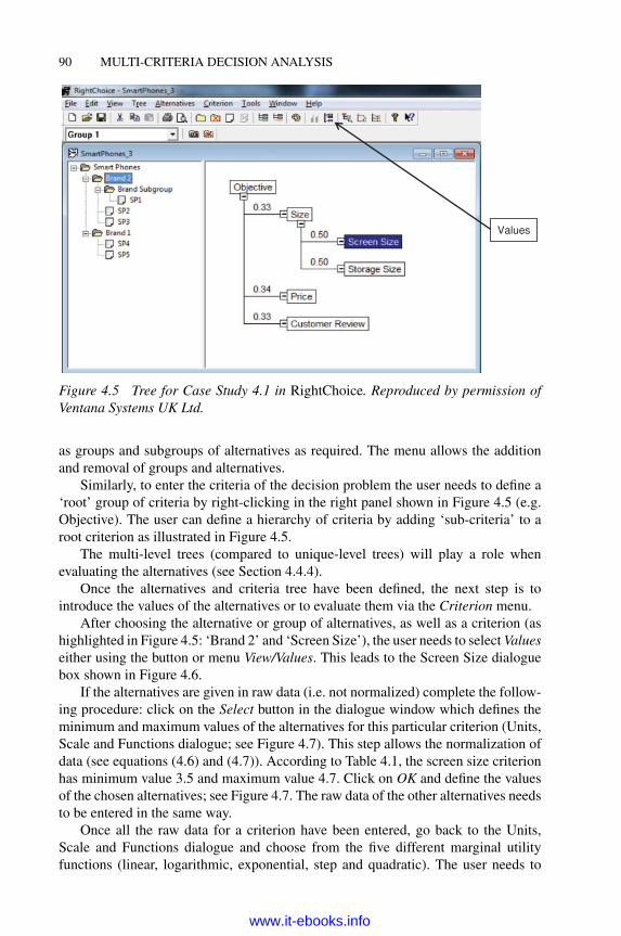
90 MULTI-CRITERIA DECISION ANALYSIS
Values
Figure 4.5 Tree for Case Study 4.1 in RightChoice. Reproduced by permission ofVentana Systems UK Ltd.
as groups and subgroups of alternatives as required. The menu allows the additionand removal of groups and alternatives.Similarly, to enter the criteria of the decision problem the user needs to define a
‘root’ group of criteria by right-clicking in the right panel shown in Figure 4.5 (e.g.Objective). The user can define a hierarchy of criteria by adding ‘sub-criteria’ to aroot criterion as illustrated in Figure 4.5.The multi-level trees (compared to unique-level trees) will play a role when
evaluating the alternatives (see Section 4.4.4).Once the alternatives and criteria tree have been defined, the next step is to
introduce the values of the alternatives or to evaluate them via the Criterion menu.After choosing the alternative or group of alternatives, as well as a criterion (as
highlighted in Figure 4.5: ‘Brand 2’ and ‘Screen Size’), the user needs to select Valueseither using the button or menu View/Values. This leads to the Screen Size dialoguebox shown in Figure 4.6.If the alternatives are given in raw data (i.e. not normalized) complete the follow-
ing procedure: click on the Select button in the dialogue window which defines theminimum and maximum values of the alternatives for this particular criterion (Units,Scale and Functions dialogue; see Figure 4.7). This step allows the normalization ofdata (see equations (4.6) and (4.7)). According to Table 4.1, the screen size criterionhas minimum value 3.5 and maximum value 4.7. Click on OK and define the valuesof the chosen alternatives; see Figure 4.7. The raw data of the other alternatives needsto be entered in the same way.Once all the raw data for a criterion have been entered, go back to the Units,
Scale and Functions dialogue and choose from the five different marginal utilityfunctions (linear, logarithmic, exponential, step and quadratic). The user needs to
www.it-ebooks.info

MULTI-ATTRIBUTE UTILITY THEORY 91
Scale
Figure 4.6 Evaluation of the alternatives.Reproduced by permission of VentanaSystems UK Ltd.
Figure 4.7 Dialogue box for definingthe units, scale and functions. Repro-duced by permission of Ventana SystemsUK Ltd.
specify whether the criterion is to be maximized or minimized (Graph Type in Figure4.8): this changes the shape of the utility function (compare Figure 4.7 and Figure 4.8).The user can define the convexity or concavity of the marginal utility function
by specifying the numerical parameter of the function (as illustrated in Figure 4.9)but cannot define piecewise linear marginal utility functions. This can be done inTools/Options/Functions. However, as previously mentioned, the user cannot changethe value of the parameter for different criteria once a shape is defined.
Figure 4.8 Dialogue box for defining the units, scale and functions when minimizingthe criterion. Reproduced by permission of Ventana Systems UK Ltd.
www.it-ebooks.info

92 MULTI-CRITERIA DECISION ANALYSIS
Figure 4.9 Parameters defining the utility functions. Reproduced by permission ofVentana Systems UK Ltd.
RightChoice can also be used to help the decision maker evaluate alternatives onthe criteria. The dialogue box for values (Figure 4.10) for a chosen criterion permitsthe introduction of utility values of different alternatives. Usually, the decision makerstarts by defining the worst and best alternative, to which they assign the marginalutility score of respectively 0 and 100.The weight of the criteria can easily be modified with theWalkingWeights option
by clicking on theWeights button or via View/Weights (Figure 4.11). By changing theweights, the impact on the utility scores can be visualized. The user always needs tospecify the group of criteria they want to act on. By selecting the root criterion, the
Figure 4.10 Dialogue box for the values on the screen size criterion. Reproducedby permission of Ventana Systems UK Ltd.
www.it-ebooks.info

MULTI-ATTRIBUTE UTILITY THEORY 93
Figure 4.11 Walking weights in RightChoice. Reproduced by permission of VentanaSystems UK Ltd.
user will be able to modify the first-level criteria and group-criteria (see, for instance,the left panel of Figure 4.11).
4.3.2 Results
By clicking on Frontier Analysis or going to Tools/Frontier Analysis, the user candisplay the utility scores and the ranking of alternatives for a given criterion. Theutility scores in RightChoice vary between 0 and 100, where 100 is the best score.To display the global utilities (Figure 4.12), the user needs to select the root of thecriteria (i.e. Objective in Figure 4.5).
Figure 4.12 Utility scores for the alternatives in Case Study 4.1. Reproduced bypermission of Ventana Systems UK Ltd.
www.it-ebooks.info

94 MULTI-CRITERIA DECISION ANALYSIS
Figure 4.13 Sensitivity Analysis box in RightChoice. Reproduced by permission ofVentana Systems UK Ltd.
If there are groups of alternatives defined, all the alternatives need to be draggedand dropped into the root group, otherwise the user will only be able to see the scoresper group and not for the complete set of alternatives.
4.3.3 Sensitivity analysis
RightChoice can perform a sensitivity analysis to illustrate when the ranking will bemodified after changing a specific weight value. Figure 4.13 shows the sensitivityanalysis of the global utility scores of the five smartphones when changing the pricecriterion. This graph shows that if the weight of price is lower than 0.44, then SP3has the highest score; otherwise, it is SP4. To display this window, the user needs toclick on the Sensitivity Analysis button or go to Tools/Sensitivity Analysis.Unfortunately, it is not possible to change the parameters of the marginal utility
functions (e.g. the exponent) in order to analyse their impact on the results.
Figure 4.14 Score analysis in RightChoice. Reproduced by permission of VentanaSystems UK Ltd.
www.it-ebooks.info

MULTI-ATTRIBUTE UTILITY THEORY 95
Figure 4.15 Addition/suppression of a weight group. Reproduced by permission ofVentana Systems UK Ltd.
Furthermore, the user can perform a Score Analysis (go to Tools/Sensitivity Anal-ysis) to establish for which criteria a specific alternative has not achieved a benchmarkscore.From Figure 4.14, one can see that SP1 does not reach the marginal utility score
of 50 on the customer review and storage size criteria, which are marked in red.
4.3.4 Group decision and multi-scenario analysis
In some situations the decision maker might want to define several scenarios for theirdecision problem. For each scenario (also called a weight group), the decision makercan define different weight and utility functions.The user can add/delete a new weight group via the toolbar menu as shown in
Figure 4.15 and can then modify their settings by selecting the appropriate weightgroup.Once the different scenarios have been set out, the user can define different
weights for each scenario by opening theWeights Series Overview. By going to View/Series Overview the user can access the interactive Weights Series menu as well asthe frontier analysis for the Weight Series Overview (Figure 4.16). This will allowthe user to analyse the global ranking when changing the weights of the differentscenarios.If the decision problem involves several decision makers, the group facilitator can
set out several scenarios corresponding to each decision maker’s preference setting.Each decision maker can thus be weighted differently and the final group decision isgiven in the Frontier Analysis: Weight Series Overview. Unfortunately, no automaticinsight is given about the difference in the ranking of the participants.
Exercise 4.3
In this exercise, you will solve the decision in Case Study 4.1 with the RightChoicesoftware.
Learning Outcomes
� Structure a problem in RightChoice
� Enter the preference parameters
� Understand the results
www.it-ebooks.info

96 MULTI-CRITERIA DECISION ANALYSIS
Figure 4.16 Weight Series Overview, Weights Series menu and the correspondingFrontier Analysis when several scenarios have been defined. Reproduced by permis-sion of Ventana Systems UK Ltd.
Consider Case Study 4.1, where the performance of the alternatives is given inTable 4.1. Enter the data in the RightChoice software and check that the same resultsas in Figure 4.12 are obtained.
Tasks
a) Read the description of Case Study 4.1 and open the software. Choose Newin the File menu.
b) From the Criterion menu, choose Add and insert the new criteria. For eachcriterion specify a name. From the Alternatives menu, choose Add and insertthe new alternatives. Define some groups in the decision tree and drag anddrop the alternatives and criteria into the groups (see Figure 4.5).
c) From the View menu, choose Values and edit the performance of the alterna-tives after choosing a specific criterion in the criterion tree. Enter theminimumand maximum values for the criterion considered, before specifying the scaletransformation.
d) Choose an exponential scale for the price and customer reviews criteria with20 as the exponent. Choose the linear scale for the two size criteria.
www.it-ebooks.info

MULTI-ATTRIBUTE UTILITY THEORY 97
e) Display the marginal utility scores for each criterion and check if the marginalranking corresponds to your intuition. Display the global utility score pergroup of alternatives as well as for the whole set of smartphones.
f) Is the ranking stable for any weight given to the combined size criterion?
g) At which specific weight values, given to the price criterion, will the rankingchange?
h) Find the criteria for which SP2 does not reach the benchmark of 20 byperforming a score analysis.
Answers can be found on the companion website.
4.4 In the black box of MAUT
MAUT is a method of total aggregation which computes the trade-off between cri-teria that respects the axioms of comparability, reflexivity, transitivity of choices,continuity and dominance (Beuthe and Scannella 1997). To have a family of criteriawhich consistently represents the decision maker’s preferences, it is necessary forthe criteria of F (see Section 4.3.1), defined on the set of alternatives A, to satisfy theaxioms of exhaustibility, cohesion and non-redundancy. If these axioms are fulfilled,the criteria define a so-called consistent family of criteria (Roy 1974). The use ofadditive functions is only permitted if the preferential independence is respected.Refer to Keeney and Raiffa (1976) and Vincke (1992) for more information on thistopic.Having formulated the conditions that the utility functions need to fulfil, the
shape of the utility functions must be considered. There are two different methods forconstructing the utility functions: the direct and indirect methods. Before detailingthese methods, the following considerations must be taken into account. This familyof methods enables a complete pre-order of the alternatives, which is a rich result (i.e.a score is given for each alternative of A). The scores allow the preference strengthto be assessed. On the other hand, the Pareto dominance relation only ascertains thedominating and dominated alternatives. Nothing is mentioned about the preferencestrength. Nothing can be said about efficient alternatives (i.e. alternatives that neitherdominate nor are dominated by other alternatives). The dominance relation thereforegives a poor result.The amount of information needed to build such aggregation models (through
several questions asked of the decisionmaker) is very important and the hypotheses oraxioms of this theory (existence, construction, additivity, etc. of U) are very strong.Such rich results are not always needed (e.g. a person may only want to find anordinal ranking). These considerations have led to the development of a mid-waytheory consisting of a mixture of the dominance relation and multi-attribute utilitytheory (Vincke, 1992): the outranking methods (see Chapters 6 and 7).
www.it-ebooks.info

98 MULTI-CRITERIA DECISION ANALYSIS
In the direct method, the marginal utility function U j is estimated to construct Udirectly. The decision maker evaluates the parameters by answering direct questionsabout their preferences (through ratings, rankings, preferences on lotteries whichgenerally include the choice between a certainty option and uncertain outcome butwith probable higher gain). Several questioning procedures exist (Vincke, 1989), andFishburn (1973) proposes various methods, which include probabilities, utilizationof compensations between the marginal utility functions, etc.The analyst needs to estimate this function by asking the decisionmaker appropri-
ate questions. Nevertheless, two fundamental problems are inherent to this approach(Vincke, 1992):
1. How are the marginal utility functions constructed? How can their parametersbe defined?
2. What properties should the decision maker’s preference have? Can they beestimated analytically?
To tackle these problems, indirect methods are an alternative for constructing themarginal utility functions. They estimate the utility functions with global judgements(i.e. not for each criterion) expressed by the decision maker on a learning set L. Thisis achieved if the ranking of the alternatives of L is given. The elicited parametershave to respect the given ranking. These methods imply that the criteria need to bedefined on a quantitative scale.Jacquet-Lagreze and Siskos (1982) work on the basis of the utilities additives
(UTA) method, which uses linear programming to obtain the parameters. The mainidea of this method is that the marginal utility functions can be estimated throughpiecewise linear functions. Greco et al. (2008) proposed UTAGMS, a generalization ofthe UTA method, which addresses the shortcomings of UTA. Recently Figueira et al.(2009) proposed the GRIP method, which generalizes both the UTA and UTAGMS
methods. GRIP has all of the features of UTAGMS but takes into account the additionalpreference information in the form of the comparison of intensities of preferencebetween pairs of reference actions.UTA, UTAGMS and GRIP are described in Section 4.6; other MAUT elicitation
methods can be found in Krantz et al. (1971), Jacquet-Lagreze and Siskos (1982),Beuthe and Scannella (1997), Greco et al. (2008) and Figueira et al. (2009).
4.5 Extensions of the MAUT method
4.5.1 The UTA method
The aimof theUTAmethod (Jacquet-Lagreze andSiskos 1982) is to infer themarginalutility functions of U through the ordinal ranking given by the decision maker onthe learning set L. The decision maker needs to rank the best to the worst of thealternatives of L, by giving each alternative a rank. Constraints can be imposed on themarginal utilities to respect (as much as possible) the given ranking. Properties such
www.it-ebooks.info

MULTI-ATTRIBUTE UTILITY THEORY 99
as transitivity will impose additional constraints. A brief introduction to the linearoptimization technique is given in the Appendix.TheUTA+ software implements the UTAmethod. This software has been chosen
because it is not only user-friendly, but also provides a rich output such as themarginalutility functions, which can be interactively modified based on a learning set.The software has a nice user interface but unfortunately only runs on Windows
3.1, 95, 98 and 2000. The software is available from Lamsade at Universite Paris-Dauphine (http://www.lamsade.dauphine.fr/spip.php?article250). The main reasonfor describing this old software is to give the reader an intuitive description of theelicitation process. In Section 4.6.2, the more recent softwareVisualUTA is described,which does not currently have similar advanced functionalities.In what follows, the weights are defined as
∀ j : w j ( f j ) · U j ( f j ) = u j ( f j ) (4.9)
This normalization allows us to avoid defining the weights as they are incorporatedinto the u j ( f j ) functions.Let f +
j and f −j be respectively the maximum and minimum values of the alter-
natives in set A to be ranked and the learning set L on criterion j (Figure 4.17).The interval [ f −
j , f +j ] can be subdivided into α j − 1 equal intervals where α j is a
parameter defined by the analyst (with α j ≥ 1). When a criterion accepts only dis-crete scores, this parameter can also correspond to the number of possible values forthis criterion. This allows us to define the ‘endpoints’ and which unknown marginalutility scores have to be determined by the linear program.The ith endpoint f i
j of the piecewise linear function of criterion j is defined asfollows (Figure 4.17):
f ij = f −
j +i − 1
(f +
j − f −j
)(α j − 1) (4.10)
0
1
Uj
fj
fj– fj
i+1fji
uj (fj
i)
fj+
Figure 4.17 Representation of the piecewise linear function for criterion j.
www.it-ebooks.info

100 MULTI-CRITERIA DECISION ANALYSIS
If the marginal utility scores of these endpoints are known, the utility score of anypoint in [ f −
j , f +j ] can be inserted in the following way: if f j (a) ∈ [ f i
j , f i+1j ], then
u j ( f j (a)) = u j(
f ij
) + f j (a)− f ij
f i+1j − f i
j
[u j
(f i+1
j
)− u j
(f i
j
)](4.11)
For all the alternatives of the learning set, the approximate marginal utility functionU ′, ∀a ∈ L can be calculated:
U ′(a) = U (a)+ σ (a) =q∑
j=1u j ( f j (a))+ σ (a) (4.12)
where σ (a) represents the potential error and u j ( f ij ) is unknown. The sum of all the
potential errors needs to be minimized:
Minimize G =[∑
a∈L
σ (a)
]minimize
∑a∈L
σ (a)
. (4.13)
Since the decision maker has expressed an ordinal ranking (possibly with equalrankings) on the learning set L, some new constraints (equalities and inequalities)need to be added to the utility scores of the alternatives of L to satisfy the preferenceand indifference relations as defined in (4.1) and (4.2).Given the transitivity of the utility scores, the equalities and inequalities obtained
from (4.1) can be reduced to the preference relations between equivalent classes(i.e. groups of indifferent alternatives) and the indifference relations within eachequivalence class. Suppose that there are Q equivalent classes with each n p (p =1, . . . , Q) indifferent alternatives. Then the following constraints exist:
Constraint 1. Q preference relations: for all a, b ∈ L ,
a P b ⇔ U (a) > U (b) ⇔q∑
j=1u j ( f j (a))−
q∑j=1
u j ( f j (b))+ σ (a)− σ (b) ≥ δ,
where δ is a small positive number.
Constraint 2.∑Q
p=1 n p indifference relations: for all a, b ∈ L ,
a I b ⇔ U (a) = U (b) ⇔q∑
j=1u j ( f j (a))−
q∑j=1
u j ( f j (b))+ σ (a)− σ (b) = 0.
Constraint 3. Normalized marginal utility functions are required:
q∑j=1
u j
(f +
j
)= 1.
www.it-ebooks.info

MULTI-ATTRIBUTE UTILITY THEORY 101
Constraint 4. To fulfil the monotonicity condition, the following condition needsto be added:
u j
(f i+1
j
)− u j
(f i
j
) ≥ t j , l = 1, . . . , α j − 1; j = 1, . . . q
where t j ≥ 0 constitutes an indifference threshold for each criterion j.
Constraint 5. To express the fact that potential errors are positive, feasibilityconditions on the error variables andmarginal utilities are given: ∀a ∈ L , ∀i, j ,
σ (a) ≥ 0.
Constraint 6. The utility value of the minimum value on the criterion equals zero:
u j
(f −
j
)= 0.
Constraint 7. The utility values are always greater than or equal to zero:
u j(
f ij
) ≥ 0.
To find the variables u j ( f ij ), the linear program that minimizes G, the sum of the
errors, needs to be solved subject to Constraints 1–7.The optimal marginal utility functions obtained can lead to G∗ = 0 or G∗ �= 0.
If G∗ �= 0, there is no set of utility functions compatible with the given ranking bythe decision maker. Jacquet-Lagreze and Siskos (1982) recommend increasing thenumber of endpoints (i.e. α j , j = 1, . . . , qα j ) of the marginal utility functions toavoid this problem. On the other hand, several sets of utility functions may lead tothe same value of G∗. In this situation, Jacquet-Lagreze and Siskos (1982) proposea further post-optimality analysis such that the utility functions lead to a rankingon L sufficiently ‘close’ to the reference ranking given by the user (in the sense ofKendall’s rank correlation coefficient, which measures the similarity between tworankings). These steps correspond to the choice of only one set of utility functions(although several are possible), which implies that some preference information islost (Greco et al. 2008). For more information on this topic, see Jacquet-Lagreze andSiskos (1982) and Greco et al. (2008).In theUTAmethod, themarginal utility functions are limited to linear or piecewise
linear marginal utility functions. This requires the analyst or decision maker to definethe number of endpoints for each criterion, which is cumbersome and restrictive.Finally, the decision maker needs to provide a complete ranking on the learning
set L which avoids any incomparability amongst alternatives. A way of avoiding thisproblem is to ask the decision maker to define pairwise comparisons as proposed inGreco et al. (2008).To address some of the shortcomings of UTA and in order to generalize its
approach, Greco et al. (2008) proposed UTAGMS, described in Section 4.6.2.
www.it-ebooks.info

102 MULTI-CRITERIA DECISION ANALYSIS
Exercise 4.4
In this exercise, you will learn how to use UTA+.
Learning Outcomes
� Construct the marginal utility functions using UTA+� Understand the steps required in the UTA+ software� Obtain the ranking on the basis of a learning set
� Perform a what-if analysis
Tasks
Consider the problem of the ranking of smartphones in Case Study 4.1 based on alearning set. Define the learning set of three reference alternatives: SP3, SP2 and SP4.Introduce the list of the alternatives of A and L. In other words, first introduce the
list of all alternatives regardless of whether or not they belong to the learning set.
a) Go to Problem/Edit, and add the names of the alternatives (left-hand columnin the Edition dialogue box in Figure 4.18).
b) Introduce the list of criteria (left-hand column in the Edition dialogue box inFigure 4.18). Define the settings for each criterion by clicking on Edit in theEdition dialogue box. Define the utility type: Gain or Cost (correspondingrespectively to maximizing or minimizing the criterion) and the number ofbreakpoints for the utility functions.
c) Enter the performance of the alternatives (click onEdit in the Edition dialoguebox after selecting the corresponding alternative); see Figure 4.19. Enter the
Figure 4.18 Criterion’s Info dialogue box in UTA+. Reproduced by permission ofLAMSADE.
www.it-ebooks.info
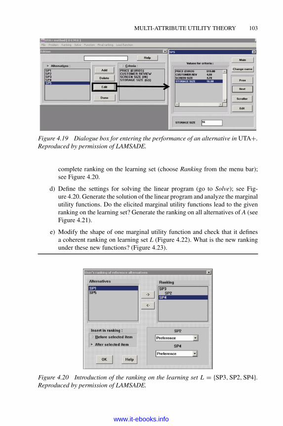
MULTI-ATTRIBUTE UTILITY THEORY 103
Figure 4.19 Dialogue box for entering the performance of an alternative in UTA+.Reproduced by permission of LAMSADE.
complete ranking on the learning set (choose Ranking from the menu bar);see Figure 4.20.
d) Define the settings for solving the linear program (go to Solve); see Fig-ure 4.20. Generate the solution of the linear program and analyze the marginalutility functions. Do the elicited marginal utility functions lead to the givenranking on the learning set? Generate the ranking on all alternatives of A (seeFigure 4.21).
e) Modify the shape of one marginal utility function and check that it definesa coherent ranking on learning set L (Figure 4.22). What is the new rankingunder these new functions? (Figure 4.23).
Figure 4.20 Introduction of the ranking on the learning set L = {SP3,SP2,SP4}.Reproduced by permission of LAMSADE.
www.it-ebooks.info

104 MULTI-CRITERIA DECISION ANALYSIS
Figure 4.21 Introduction of the parameters to solve the linear programme. Repro-duced by permission of LAMSADE.
Figure 4.22 The elicited marginal utility functions which ensure a coherent completeranking on L. Reproduced by permission of LAMSADE.
www.it-ebooks.info

MULTI-ATTRIBUTE UTILITY THEORY 105
Figure 4.23 Window to modify the shape of the marginal utility function. Reproducedby permission of LAMSADE.
4.5.2 UTAGMS
TheUTAGMS method generalizes theUTAmethod in three aspects (Greco et al. 2008).Unlike the UTA method which uses only one set of piecewise linear functions, theUTAGMS method can take all additive value functions compatible with the preferenceinformation provided by the decision maker (see Figure 4.24). The only hypothesison these functions is that they are non-decreasing (this generalizes the piecewiselinearity). Moreover, the ranking on the learning set L does not need to be complete(i.e. there might be incomparable alternatives in L).The software VisualUTA that supports UTAGMS is available from http://idss.cs
.put.poznan.pl/site/visualuta.html and will be described briefly in Exercise 4.5.Similarly to UTA, the UTAGMS method takes input from the decision maker in
the form of an ordinal ranking on the learning set L. The ranking can be a partial pre-order: the decision maker provides pairwise comparisons between the alternatives ofL. Non-decreasing additive utility functions are elicited such that they are compatiblewith the given preference information.To determine the utility function values the following constraints need to be
respected (analogous to Constraints 1–7):
1. Constraint 1 takes into account the user preferences on the learning set:
∀a, b ∈ L :
{aPb ⇔ U (a) > U (b)aIb ⇔ U (a) = U (b).
0
1
c
fj
Figure 4.24 Marginal utility functions in UTAGMS.
www.it-ebooks.info
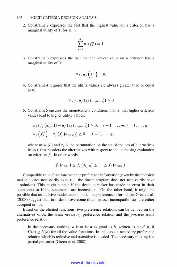
106 MULTI-CRITERIA DECISION ANALYSIS
2. Constraint 2 expresses the fact that the highest value on a criterion has amarginal utility of 1, for all i:
q∑j=1
u j ( f +j ) = 1.
3. Constraint 3 expresses the fact that the lowest value on a criterion has amarginal utility of 0:
∀ j : u j
(f −
j
)= 0.
4. Constraint 4 requires that the utility values are always greater than or equalto 0:
∀i, j : u j(
f j(aτ j (i−1)
)) ≥ 0
5. Constraint 5 ensures the monotonicity condition, that is, that higher criterionvalues lead to higher utility values:
u j(
f j(aτ j (i)
)) − u j(
f j(aτ j (i−1)
)) ≥ 0, i − 1, . . . , m; j = 1, . . . , q,
u j
(f +
j
)− u j
(f j
(aτ j (m)
)) ≥ 0, j = 1, . . . , q,
where m = |L| and τ j is the permutation on the set of indices of alternativesfrom L that reorders the alternatives with respect to the increasing evaluationon criterion f j . In other words,
f j(aτ j (1)
) ≤ f j(aτ j (2)
) ≤ . . . ≤ f j(aτ j (m)
).
Compatible value functions with the preference information given by the decisionmaker do not necessarily exist (i.e. the linear program does not necessarily havea solution). This might happen if the decision maker has made an error in theirstatements or if the statements are inconsistent. On the other hand, it might bepossible that an additive model cannot model the preference information. Greco et al.(2008) suggest that, in order to overcome this impasse, incompatibilities are eitheraccepted or not.Based on the elicited functions, two preference relations can be defined on the
alternatives of A: the weak necessary preference relation and the possible weakpreference relation.
1. In the necessary ranking, a is at least as good as b, written as a �N b, ifU (a) ≥ U (b) for all the value functions. In this case, a necessary preferencerelation which is reflexive and transitive is needed. The necessary ranking is apartial pre-order (Greco et al. 2008).
www.it-ebooks.info

MULTI-ATTRIBUTE UTILITY THEORY 107
2. In the possible ranking, a is at least as good as b, written as a �P b, ifU (a) ≥ U (b) for at least one value function compatible with the ranking onL. The possible ranking is ‘strongly’ complete (Greco et al. 2008): there is noincomparability in the possible ranking.
Consider the notation a b ⇔ U (a) ≥ U (b). This leads to
∀a, b ∈ L : a b ⇒ a N b and a Pb ⇒ not (b P a).
The necessary preference relation is included in the possible preference relation(P⊇N ): if U (a) ≥ U (b) for all possible value functions U, then there is at leastone compatible value function U ′ such that U ′(a) ≥ U ′(b).The necessary ranking can be considered as robust with respect to the provided
ranking on L, since the preference relations between two alternatives hold for anyvalue function. When no preference relation exists between a pair of alternatives, thenecessary ranking corresponds to the weak dominance relation and the preferencerelation is a complete relation.The authors suggest using the UTAGMS method interactively with the decision
maker by adding alternatives to learning set L, since this will be taken into accountby the model in the next iteration.In order to compute the binary relations N and P for two alternatives a, b of
A, proceed as follows (Greco et al. 2008):
1. Reorder the alternatives from L ∪ {a, b} from the worst to the best on criterionf j , and note this permutation π j :
f j(aπ j (1)
) ≤ f j(aπ j (2)
) ≤ . . . ≤ f j(aπ j (η)
), (4.14)
where η = |L ∪ {a, b}|. This value can be equal to m + 2, m + 1 or m accord-ing to the union operator.
2. The endpoints of the utility functions are defined as follows: ∀ j = 1, . . . , q,
f 0j = f −j ; f i
j = f j(aπ j (i)
); . . . ; f η+1
j = f +j . (4.15)
3. The following constraints, depending on a and b, need to be satisfied fori = 1, . . . , η + 1 and j = 1, . . . , q .
Constraint 8
∀a, b ∈ L :
{aPb ⇔ U (a) > U (b)+ σ
aIb ⇔ U (a) = U (b)∀i, j : u j
(f 0j
) = 0; j = 1, . . . , q,
where σ is random small positive number.
Constraint 9
u j(
f ij
) − u j
(f i−1
j
)≥ 0; i = 1, . . . , η + 1.
www.it-ebooks.info

108 MULTI-CRITERIA DECISION ANALYSIS
Constraint 10
q∑j=1
u j ( f η+1j ) = 1.
1. If the solution space is not empty:
◦ a �N b ⇔ d(a, b) ≥ 0 where d(a, b)min{U (a)− U (b)} respectingConstraint 10;
◦ a �P b ⇔ D(a, b) ≥ 0 where D(a, b) = max{U (a)− U (b)} respectingConstraint 10.
Let us remark that not all the distances d(a,b) and D(a,b) need to be computed,as explained in Greco et al. (2008).
The authors of the UTAGMS method have proposed an extension where the deci-sion maker can assign confidence levels to pairwise comparisons. This yields valuednecessary preference relations and valued possible preference relations.
Exercise 4.5
In this exercise, you will learn how to use VisualUTA.
Learning Outcomes
� Input the data into VisualUTA
� Understand the results of VisualUTA
Tasks
Consider the problem of the ranking of smartphones in Case Study 4.1 based on alearning set. As in Exercise 4.4, define the learning set of three reference alternatives:SP3, SP2 and SP4.Input the alternatives in the same list regardless of whether they belong to ranking
set A or learning set L.
1. For this task, go to the Alternatives panel on the left of the screen, input thename of the alternative and then click on the ‘+’ button (see Figure 4.25).
2. Input the list of criteria (at the bottom left of the screen). Click on the ‘+’button in the Criteria Set panel, specify the name, the description and thetype of criterion. Choose Gain if the criterion has to be maximized or Costotherwise (see Figure 4.26).
www.it-ebooks.info

MULTI-ATTRIBUTE UTILITY THEORY 109
Figure 4.25 Inputting the set of alternatives A and L in VisualUTA. Reproduced bypermission of Roman Słowinski.
3. Enter the performance of the alternatives by clicking on the toolbar menu,which opens the evaluation grid (see Figure 4.26). Define the set of referencealternatives as well as their corresponding ranking by dragging and droppingthe reference alternatives from the Alternatives Set panel to the Referenceranking panel. Modify the rank of a chosen reference alternative with the ‘+’and ‘−’ button (Figure 4.27) if necessary.
4. Solve the problem by pressing F5, going to Calculate/Solve or by click-ing on the calculator icon in the toolbar. This leads to the ‘Final Rankingworked out with UTA MD’ (dominance model), the ‘Alternatives compari-son matrix’ and the ‘Resulting preference graphs worked out with the UTAGMS’ (Figure 4.28). Is the ranking similar to the deduced ranking obtained in
Figure 4.26 Inputting the set of criteria in VisualUTA. Reproduced by permissionof Roman Słowinski.
www.it-ebooks.info

110 MULTI-CRITERIA DECISION ANALYSIS
Figure 4.27 Inputting the ranking on the learning set L = {SP3,SP2,SP4}. Repro-duced by permission of Roman Słowinski.
Figure 4.28 Display of the results of the Visual UTA software. Reproduced bypermission of Roman Słowinski.
www.it-ebooks.info

MULTI-ATTRIBUTE UTILITY THEORY 111
Exercise 4.4? What are the relationships between the alternatives in the pref-erence graphs?
5. Change the settings (the delta threshold of the linear programming correspond-ing to σ in Constraint 8) and epsilon used when computing the ‘distances’d(a, b) and D(a, b) by going to Calculate/Options. What is the impact ofthose parameters on the ranking?
Members of the Laboratory of Intelligent Decision Support of the Institute of Com-puting Science of the Poznan University of Technology have recommended settingthe value of epsilon slightly lower than delta due to the calculation errors which usu-ally occur when solving linear programs. If the delta and epsilon thresholds are smallenough, an outranking relation is defined for (almost) all compatible value functions.For greater values of these thresholds, a model is developed concerning just a set ofvalue functions, for which the relations of preference between reference alternativesare clear (the difference between the value of two alternatives is greater than delta).
4.5.3 GRIP
The generalized regression with intensities of preference (GRIP) method belongsto the class of methods based on indirect preference information and the ordinalregression paradigm. In other words, GRIP enables the ranking of a finite set ofalternatives A based on a partial pre-order and intensities of preferences on a subsetof reference actions L given by the decision maker. Currently, there is no dedicatedsoftware that implements the GRIP method, but see Figueira et al. (2009) for moretechnical information and implementation steps of the method.In contrast to other elicitation methods, the given preference information in GRIP
does not need to be complete. The decision maker can provide some comparisonsbetween the reference actions. A complete pre-order as in UTA is thus not required.Moreover, these comparisons can be considered on all criteria (i.e. comprehensively)or on specific criteria (i.e. partially). The decision maker can specify comparisons ofstrengths of preferences between some pairs of reference actions: for example, ‘x ispreferred to y at least as much as w is to z’ or ‘x is preferred to y at least as much asw is to z, on criterion fi ’. GRIP can be seen as a generalization of both the UTA andUTAGMS methods.The indirect preference information given by the decision maker is interpreted as
a set of ordinal regression constraints (analogously as in UTA and UTAGMS), whichdefine a compatible set of additive value functions. The obtained additive valuefunctions lead to the following preference relations in A and intensities of preferencefor these relations:
� The necessary and possible rankings for all pairs of actions (x, y) ∈ A × A.
� The necessary and possible rankings with respect to the comprehensive inten-sities of preferences for all ((x, y), (w, z)) ∈ A × A × A × A.
www.it-ebooks.info

112 MULTI-CRITERIA DECISION ANALYSIS
� The necessary and possible rankings with respect to the partial intensities ofpreference for all ((x, y), (w, z)) ∈ A × A × A × A and for all criteria fi ∈ F .
In practice, the necessary and possible rankings are the most useful outputs for thedecision maker.The input given by the decision maker in GRIP can be considered as similar to the
information required by AHP (see Chapter 2). In both methods, the decision makercan compare pairwise alternatives on a particular criterion with respect to strength ofpreferences. This permits the comparison of AHP with GRIP in respect to a singlecriterion. In AHP the strength of preference (given on a scale from 1 to 9) is translatedinto quantitative terms by for instance the principal eigenvectors, which is not alwayseasy to justify. In GRIP, themarginal value functions are a numerical representation ofthe original qualitative-ordinal information without any intermediate transformationinto quantitative terms (Figueira et al. 2009).Furthermore, in GRIP weights do not need to be elicited (contrary to AHP) since
the marginal value functions are expressed on the same preference scale and, as aresult, the value functions can be summed. The elicited marginal value functions canbe based on judgements which involve all the criteria simultaneously. For a moredetailed comparison of GRIP and AHP, see Figueira et al. (2009).GRIP can also be compared to MACBETH (see Chapter 5), which takes into
account a preference order of actions and strength of preference comparisons onspecific criteria (Figueira et al. 2009). Based on the preference information provided,MACBETHbuilds an interval scale for each criterion bymeans of linear programmingmodels. GRIP and MACBETH both deal with qualitative judgements to build anumerical representation of the preferences. However, GRIP is more general thanMACBETH since the comparisons in GRIP can involve all criteria simultaneously.As explained in Figueira et al. (2009), the structure of strength of preference inMACBETH is a particular case of that in GRIP. For a more detailed comparison ofGRIP and MACBETH, see Figueira et al. (2009).
References
Beuthe, M., and Scannella, G. (1997). Comparative analysis of UTAs multicriteria methods.European Journal of Operational Research, 130, 246–262.
Figueira, J., Greco, S., and Slowinski, R. (2009). Building a set of additive value functionsrepresenting a reference preorder and intensities of preference: GRIP method. EuropeanJournal of Operational Research, 195, 460–486.
Fishburn, P. (1973). The Theory of Social Choice. Princeton, NJ: Princeton University Press.
Greco, S., Mousseau, V., and Slowinski, R. (2008). Ordinal regression revisited: Multiplecriteria ranking using a set of additive value functions. European Journal of OperationalResearch, 191, 416–436.
Jacquet-Lagreze, E., and Siskos, J. (1982). Assessing a set of additive utility functions formulticriteria decision-making, theUTAmethod.European Journal of Operational Research,10, 151–164.
www.it-ebooks.info

MULTI-ATTRIBUTE UTILITY THEORY 113
Keeney, R., and Raiffa, H. (1976). Decisions with Multiple Objectives: Preferences and ValueTrade-offs. New York: John Wiley & Sons, Inc.
Krantz, D., Luce, D., Stuppens, P., and Tvesky, A. (1971). Foundations of Measurement.New York: Academic Press.
Roy, B. (1974). Criteres multiples et modelisation des preferences: l’apport des relations desurclassement. Revue d’Economie Politique, 1, 1–44.
Vincke, P. (1989). L’aide multicritere a la decision. Brussels: Edition Ellipses – Editions deL’Universite Libre.
Vincke, P. (1992).Multicriteria Decision Aid. New York: John Wiley & Sons, Inc.
Zopounidis, M. and Doumpos, C. (2002).Multicriteria Decision Aid Classification Methods.Dordrecht: Kluwer Academic Publishers.
www.it-ebooks.info

5
MACBETH
5.1 Introduction
This chapter explains the theory and practical uses of MACBETH. You will learnhow to use the M-MACBETH software, which helps to structure problems and cal-culate the attractiveness (scores) of the options (choices). Section 5.3 is designedfor readers interested in the methodological background of MACBETH. In orderto understand this section, an understanding of linear programming is needed (seethe Appendix).The companion website provides illustrative examples withMicrosoft Excel, and
case studies and an example with MACBETH.
5.2 Essential concepts of MACBETH
MACBETH stands for ‘Measuring Attractiveness by a Categorical Based EvaluationTechnique’. From a user point of view, MACBETH has many similarities with AHP.A novice may even not see the difference. Both methods are based on pairwisecomparisons entered by the user, but MACBETH uses an interval scale and AHPadopts a ratio scale (Example 5.1). The calculation process behind AHP (Section 2.4)is different from MACBETH as described in Section 5.3.
Example 5.1 Consider the price of a Chinese (£1000) and Japanese caterer (£5000)for a conference that you organize. The pairwise comparisons inAHPandMACBETHare performed differently. AHP uses a ratio scale, 50001000 = 5, whichmeans that the priceof the Japanese caterer is 5 times as expensive. MACBETH uses an interval scale:5000 – 1000 = £4000. The decision maker should therefore evaluate the difference(£4000) between the two prices.
Multi-Criteria Decision Analysis: Methods and Software, First Edition. Alessio Ishizaka and Philippe Nemery.© 2013 John Wiley & Sons, Ltd. Published 2013 by John Wiley & Sons, Ltd.
www.it-ebooks.info

MACBETH 115
Value tree
Caterer selection
Consumables
Drinks
Food
Service
Quality
Price
Reliability
Flexibility
Figure 5.1 Tree of the decisions. Reproduced by permission of BANA ConsultingLda.
The user of MACBETH will need to complete three steps in order to obtain theranking of the options. As with any MCDA method, the first step is to structure theproblem, followed by entering pairwise comparisons into a judgement matrix. Ifthe matrix is sufficiently consistent, the attractiveness can be calculated, otherwisethe user is obliged to revise their judgements. Finally, an optional sensitivityanalysis is recommended. This task is largely facilitated by the supporting softwareM-MACBETH.
5.2.1 Problem structuring: Value tree
MACBETH structures the problem in a tree or hierarchy, but makes a distinctionbetween criteria and non-criteria nodes. Non-criteria nodes are included in the treeto help with the evaluation of criteria nodes but are not directly influential in thedecision. They act only as comments to structure the problem and therefore will notbe evaluated. Only one-criterion nodes can be set between the overall node (top ofthe tree) and the leaves (bottom of the tree). For example, in Figure 5.1, only Qualityis set as a criterion between the top of the tree (Caterer selection) and the leaf (Food).It would have been impossible to set another node (Consumables, Service, Drinks orFood) as criterion under the node Quality. For those who are familiar with AHP, thisis unusual. Indeed, if there is only one criterion between the overall node and leaf,then the value tree is not equivalent to the AHP criteria tree. The structure can bereduced to one level with no subcriteria.This chapter will consider a caterer selection problem in order illustrate the
different steps of the MACBETH process (Case Study 5.1).
www.it-ebooks.info

116 MULTI-CRITERIA DECISION ANALYSIS
Case Study 5.1
A university organizes a three-day conference and needs to select a caterer toprovide the lunches. It is expected to have around 200 participants, but the exactnumber is uncertain. The schedule is very tight and a delay in the service woulddisrupt all the presentations in the afternoon. The organizing committee contem-plates four options:
a) Internal catererThe university has a catering service,which ismore expensive than externalcaterers. It provides a large range of sandwiches. It has been used to caterfor other conferences, and its service is reliable. It is very flexible in thatthe number of lunches can be adjusted the day before.
b) Indian catererA member of the organizing committee has used an Indian caterer for aprivate party. It produced high-quality food for a reasonable price. How-ever, it does not have previous experience of catering for large numbersand may be a risky solution.
c) Chinese catererA Chinese fast food restaurant also provides catering for big events. Itsservice has been used successfully at past conferences as an alternative tothe internal caterer. Its food quality is average and its price is low. It isvery flexible with regard to the number of lunches, as the food is preparedon the spot in large woks.
d) Japanese catererA Japanese caterer has just opened. Its main dishes are sushi. It has thesame price range as the internal caterer but offers higher-quality food. As itis a new business, its flexibility and reliability in providing a large numberof lunches is not known.
The decision will thus be based on four criteria given in Table 5.1.
Table 5.1 List of criteria.
Criteria Explanation
Quality Quality of the food and servicePrice Cost of the serviceReliability Capacity to work on a tight schedule for the conferenceFlexibility How easily they adjust the number of lunches for
additional participants
Figure 5.1 represents the tree, generally referred to as a ‘value tree’, from CaseStudy 5.1. The top node of the tree contains the overall goal. Quality, Price, Reliabilityand Flexibility are criteria nodes (in bold in Figure 5.1). Consumables, Service,Drinks
www.it-ebooks.info

MACBETH 117
and Food are non-criteria but essential information in order to evaluate the Qualitycriterion.
5.2.2 Score calculation
After the problem-structuring phase of previous section, three types of scores haveto be calculated:
� Weighting criteria. These measure the attractiveness of each criterion in rela-tion to the top goal.
� Scores of options. These represent the attractiveness of an option to onespecific criterion.
� Overall score of options. Criteria weight and option scores are only interme-diate results used to calculate the overall score of options. Whilst the score ofoptions ranks themwith regard to a single criterion, the overall score of optionsranks them with regard to all criteria and consequently to the overall goal.
The relative attractiveness of each criterion is evaluated pairwise. Then, the optionsare compared pairwise with regard to each criterion. In Case Study 5.1, five differentjudgement matrices are required: four local scores of options with regard to eachcriterion and one weight criteria score.MACBETH is a pairwise comparison based method on an interval scale. The user
will need to provide only qualitative judgements about the difference of attractivenessbetween two options. The traditional MACBETH offers seven semantic categoriesfor the evaluation (Table 5.2) but other verbal scales can be imagined. For example,a ‘4’ would read as ‘Option A is moderately more attractive than Option B’.It is recommended to first order the elements to be evaluated. This is not a
mandatory step but it helps to ensure consistency when filling the judgement matrix.Your judgements will be in an increasing order from right to left and from the bottomto the top of your matrix (see Table 5.3). Only the upper triangle of the matrix needsto be completed because the lower triangle is the reverse and can be deduced from theupper triangle. As in AHP (Chapter 2), the redundancy of information leads to a gainin precision but requires a higher effort, especially for a large number of decisionelements.
Table 5.2 Seven semantic categories.
Semantic categories Quantitative scale
no 1very weak 2weak 3moderate 4strong 5very strong 6extreme 7
www.it-ebooks.info

118 MULTI-CRITERIA DECISION ANALYSIS
Table 5.3 Matrix of judgements.
Quality Price Reliability Flexibility
Quality no very weak weak moderatePrice no very weak weakReliability no weakFlexibility no
Example 5.2 In order to weight the criteria of Case Study 5.1, first rank the criteriain order of importance. In this case, quality is the most important criterion, followedby price, reliability and, finally, flexibility. Then the matrix of judgements (Table 5.3)expresses the difference in attractiveness between the criteria. For example, qualityis slightly more important than price. The main diagonal has no values because acriterion does not need to be compared to itself.
From such a matrix of judgements, the software will calculate the weights andscores of options. First, the least attractive option/criterion is grounded to 0. Then,lists of conditions reflecting the user’s judgement in Table 5.3 are set. A linearoptimization is used to minimize the score of the most attractive option/criterion.However, as several solutions may exist, the scores can be readjusted in accordancewith the user’s feelings (see Figure 5.10), while still fulfilling the semantic categoryconstraint conditions. This easy readjustment is done in the software with a graphicalthermometer bar. Advanced readers can refer to Section 5.4 to understand how thescores are calculated.Finally,MACBETH aggregates theseweighted scores additively in order to derive
the overall score of options. Unlike toAHP,MACBETH requires a high consistency inorder to be able to calculate scores. Therefore, each time a judgement is provided, thesoftware will verify the consistency and suggest changes to resolve any inconsistency.The consistency check is explained in the next section.
5.2.3 Incompatibility check
When filling a judgement matrix, the decision maker may introduce incompatiblejudgements. This can occur with comparative and semantic judgements. A compar-ative judgement is given between two actions on a semantic category (Table 5.2). Itis the judgements that a decision maker enters in the matrix. A semantic judgementis the comparison between two comparative judgements. It is the difference betweentwo judgements entered into a matrix.
Example 5.3
Comparative judgements:
� A is weakly more attractive than B.
� C is moderately more attractive than B.
www.it-ebooks.info

MACBETH 119
Attractivenesson one criterion
B
A
C
Figure 5.2 Semantic judgement difference of attractiveness B – C > A – C.
Semantic judgement:
� The difference in attractiveness between C and B (moderate) is bigger than thedifference in attractiveness between A and B (weak).
There are two types of incompatibility in MACBETH: incoherence and semanticinconsistency.
Incoherence inconsistency. There are four cases where a conflict can arise between acomparative judgement and a semantic judgement.
� In Figure 5.2, the semantic judgement difference of attractiveness betweenB and C is higher than that of A and C (B – C > A – C). This would be‘incoherent’ with the comparative judgement A better than B (A > B).
� In Figure 5.3, the semantic judgement difference of attractiveness between Band C is higher than the difference of attractiveness between B and A (B –C > B – A). This would be ‘incoherent’ with the comparative judgement Cbetter than A (C > A).
� In Figure 5.2, the semantic judgement difference of attractiveness between Band C is higher than the difference of attractiveness between A and C (B –C > A – C). This would be ‘incoherent’ with the comparative judgement A isequal to B (A = B).
� In Figure 5.3, the semantic judgement difference of attractiveness between Band C is higher than the difference of attractiveness between B and A (B –C > B – A). This would be ‘incoherent’ with the comparative judgement Cequal to A (C = A).
www.it-ebooks.info

120 MULTI-CRITERIA DECISION ANALYSIS
Attractivenesson one criterion
B
A
C
Figure 5.3 Semantic judgement difference of attractiveness B – C > B – A.
B
C
A D
weak
very weak
very strong
moderate
Figure 5.4 Graph of semantic inconsistency.
Semantic inconsistency. The semantic inconsistency is tested by a linear program thatcan be found in Bana e Costa et al. (2005). Basically, it tests that ‘two paths’ betweentwo points (representing the preference strength) should have the same ‘length’. Forexample, the graph in Figure 5.4 presents a semantic inconsistency because A – B >
A – C and B – D > C – D, therefore the path A-B-D is much longer than A-C-D.However, the linear program accepts surprising cases as in Figure 5.5, where the pathA-B-D is much longer than A-C-D.
B
C
A D
very weak
very weak
extreme
very weak
Figure 5.5 Consistent graph.
www.it-ebooks.info
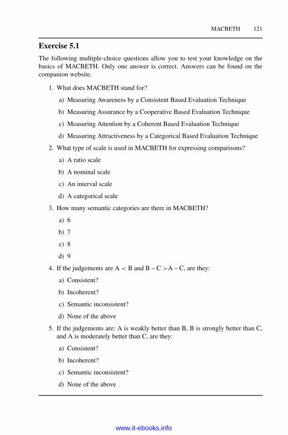
MACBETH 121
Exercise 5.1
The following multiple-choice questions allow you to test your knowledge on thebasics of MACBETH. Only one answer is correct. Answers can be found on thecompanion website.
1. What does MACBETH stand for?
a) Measuring Awareness by a Consistent Based Evaluation Technique
b) Measuring Assurance by a Cooperative Based Evaluation Technique
c) Measuring Attention by a Coherent Based Evaluation Technique
d) Measuring Attractiveness by a Categorical Based Evaluation Technique
2. What type of scale is used in MACBETH for expressing comparisons?
a) A ratio scale
b) A nominal scale
c) An interval scale
d) A categorical scale
3. How many semantic categories are there in MACBETH?
a) 6
b) 7
c) 8
d) 9
4. If the judgements are A < B and B – C >A – C, are they:
a) Consistent?
b) Incoherent?
c) Semantic inconsistent?
d) None of the above
5. If the judgements are: A is weakly better than B, B is strongly better than C,and A is moderately better than C, are they:
a) Consistent?
b) Incoherent?
c) Semantic inconsistent?
d) None of the above
www.it-ebooks.info

122 MULTI-CRITERIA DECISION ANALYSIS
5.3 Software description: M-MACBETH
MACBETH is supported by M-MACBETH. As far as we know there is no othercommercial software for MACBETH, although a template in Microsoft Excel canbe generated (Section 5.4). M-MACBETH is a user-friendly program with intuitivegraphical user interfaces that automatically computes attractiveness and possibleinconsistencies, as well as ways to process a sensitivity analysis. M-MACBETH hasbeen translated into four languages (English, French, Portuguese and Spanish).This section describesM-MACBETH and the essential functions of the graphical
user interface. A full tutorial can be downloaded from the M-MACBETH website:http://www.m-macbeth.com/en/downloads.html.A free trial version can be downloaded from http://www.m-macbeth.com/. This
version is limited to five criteria and five options. It is not necessary to know howscores are calculated, but only what should be ranked.In this section the three steps introduced in Section 5.2 will be followed.
5.3.1 Problem structuring: Value tree
Nodes are entered by right-clicking on the parent node followed by selecting Add anode. By default all nodes are set as non-criteria. In order to change a non-criterion toa criterion node, right-click on the node and select node properties. Select to comparethe options of the problem only or the options and two benchmark references. Thesetwo benchmarks are by default the upper and lower reference. They can easily bechanged, for example, to good and neutral. These two benchmarks are virtual andoptional. They permit two reference points for entering judgements. The drawbackis that the number of judgements required increases.Nodes can also be directly compared on qualitative or quantitative performance-
level scales. For example, in Figure 5.6, five qualitative levels for price are defined.Options are entered via the menu Options/Define.
5.3.2 Evaluations and scores
Two types of evaluation are possible on a qualitative or quantitative performance-level scale: pairwise judgement of the options or direct evaluation. The choice of theevaluation technique needs to be done when setting the criterion nodes (see Section5.3.1). In order to enter the assessments for the options or performance levels, clickon the criterion node and choose Judgements. The evaluation of the criteria can alsobe done in a matrix of judgements by selecting the menuWeighting/Judgements.The evaluation of the options (Figure 5.7), performance levels (Figure 5.8) and
criteria follows a similar process. It is recommended to order the options by selectingand dragging them up or down in the column of the judgement matrix in decreasingorder of attractiveness (Figure 5.6). Only n – 1 independent evaluations are requiredas the others can be deduced by transitivity. However, it is better to fill the uppertriangle of the matrix using the semantic categories (Table 5.2). If the decision makeris unsure about the exact category, they can select two or more successive categories
www.it-ebooks.info

MACBETH 123
Figure 5.6 Qualitative levels. Reproduced by permission of BANA Consulting Lda.
as in Figure 5.8. Between low and high price, the difference is evaluated from verystrong to extreme. The best option/level will be highlighted in green whilst the worstwill be in blue.The calculation of scores is done by clicking on the seventh button shown in
Figure 5.7 and Figure 5.8. The scores are scaled so that the upper reference is 100and the lower reference is 0 (Figure 5.9). If the two reference levels are not defined,
Figure 5.7 Matrix of judgements for options with regard to quality. Reproduced bypermission of BANA Consulting Lda.
www.it-ebooks.info

124 MULTI-CRITERIA DECISION ANALYSIS
Figure 5.8 Matrix of judgements for performance levels of price. Reproduced bypermission of BANA Consulting Lda.
Figure 5.9 MACBETH numerical scale. Reproduced by permission of BANA Con-sulting Lda.
www.it-ebooks.info

MACBETH 125
Figure 5.10 MACBETH weighting scale. Reproduced by permission of BANA Con-sulting Lda.
the software automatically assigns the scores 0 and 100 to the two endpoints of thescale. The normalization of the weights is different from that of the options (Figure5.10). They are normalized to 100 (the sum of the weights adds up to 100).
M-MACBETH allows the scores to be readjusted, whilst being compatible withthe judgements provided in the matrix. The permissible interval is shown in red onthe left part of the thermometer bar and options can be dragged up or down the axis(Figure 5.9 and 5.10).In the direct evaluation of options, the performance levels calculated in Figure
5.8 need to be allocated to the options by choosing Options/Table of performances(Figure 5.11).
5.3.3 Incompatibility check
When contradictory evaluations are entered, M-MACBETH will detect them andissue a warning. For example, in Figure 5.12, the judgement between the Indian andChinese caterers being weak is inconsistent with the previously entered judgements.
www.it-ebooks.info

126 MULTI-CRITERIA DECISION ANALYSIS
Figure 5.11 Performance table. Reproduced by permission of BANA Consulting Lda.
Figure 5.12 Matrix with inconsistent judgements. Reproduced by permission ofBANA Consulting Lda.
The red arrow pointing down explains that the judgement should be decreased andthe number indicates the number of categories. In Figure 5.12, the first suggestionimplies that the judgement of very strong between the Indian and internal caterersshould be reduced to weak. To see the other suggestions, click on the fourth button.By clicking on the second button, the contradictions are explained. Figure 5.13
explains the incompatibility of the matrix of Figure 5.12. The first problem is anincoherence and the second one is a semantic inconsistency (see Section 5.2.3).
Figure 5.13 Incompatibility explanation. Reproduced by permission of BANA Con-sulting Lda.
www.it-ebooks.info

MACBETH 127
Figure 5.14 Overall scores. Reproduced by permission of BANA Consulting Lda.
5.3.4 Results
Selecting Options/Table of scores displays the table of results (Figure 5.14). Thistable contains the overall scores and scores with regard to each criterion. The scoresare normalized for each criterion in order that the most attractive option has a scoreof 100 and the least attractive option receives 0. The internal caterer is the mostattractive option.A further analysis of the options can be done graphically. The difference between
the profiles for any two options can be viewed (go to Options/Difference profiles).For example, in Figure 5.15, the internal caterer is compared to the Indian caterer.If the quality of the Internal caterer is far less attractive than the Indian caterer, itcompensates this deficit with more attractive price, reliability and flexibility.Another way to analyze the results is to use a two-dimensional graph, where each
axis represents a criterion (go to Options/XY Map). In Figure 5.16, the options arerepresented according to their attractiveness on the price and quality criteria. It can beseen that the Japanese caterer has a high quality but is not attractive on the price. Onthe other hand, the internal caterer has an attractive price and a low quality. The linerepresents the efficient frontier. In this case, the Chinese caterer is a dominated option.
5.3.5 Sensitivity analysis
A static graphical sensitivity analysis is available in M-MACBETH (go to Weight-ing/Sensitivity analysis by weight). It allows the impact of the change on one criterionweight on the overall score to be observed. For example, in Figure 5.17, the impactof the quality criterion weight is plotted. If the weight given to quality is over 46.2,the Indian caterer will be overall the most attractive option instead of the internalcaterer. If the weight is more than 80, than the Japanese caterer becomes the mostattractive option.
5.3.6 Robustness analysis
The robustness analysis allows exploration if the proposed solution remainsunchanged after a variation in the weights of the criteria. This analysis is important
www.it-ebooks.info

128 MULTI-CRITERIA DECISION ANALYSIS
Figure 5.15 Profiles difference. Reproduced by permission of BANA Consulting Lda.
in an uncertain problem with imprecise information. In Figure 5.18, a 5% uncertaintyis used for each weight of the criterion. Three types of symbols can be found:
� The symbol means that the global preference of the line action over thecolumn action does not depend on any combination of weight criteria.
� The symbol means that the preference of the line action over the columnaction is not modified if there is less than the defined uncertainty in the weightalteration.
� The ? symbol means that the preference of the line action over the columnaction can be modified if there is less (or more) than the defined uncertainty inthe weight alterations.
For example, in Figure 5.18 the Indian caterer is always preferred over theJapanese caterer and is preferred over the Chinese and internal caterer if the weightalteration is below 5%.
www.it-ebooks.info

MACBETH 129
Figure 5.16 Comparison of scores on two criteria. Reproduced by permission ofBANA Consulting Lda.
Figure 5.17 Sensitivity analysis. Reproduced by permission of BANA ConsultingLda.
www.it-ebooks.info
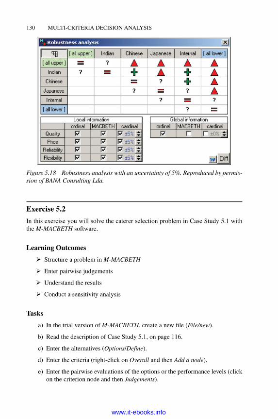
130 MULTI-CRITERIA DECISION ANALYSIS
Figure 5.18 Robustness analysis with an uncertainty of 5%. Reproduced by permis-sion of BANA Consulting Lda.
Exercise 5.2
In this exercise you will solve the caterer selection problem in Case Study 5.1 withthe M-MACBETH software.
Learning Outcomes
� Structure a problem inM-MACBETH
� Enter pairwise judgements
� Understand the results
� Conduct a sensitivity analysis
Tasks
a) In the trial version of M-MACBETH, create a new file (File/new).
b) Read the description of Case Study 5.1, on page 116.
c) Enter the alternatives (Options/Define).
d) Enter the criteria (right-click on Overall and then Add a node).
e) Enter the pairwise evaluations of the options or the performance levels (clickon the criterion node and then Judgements).
www.it-ebooks.info

MACBETH 131
f) Enter the pairwise evaluations for the criteria (Weighting/Judgements).
g) Read the overall ranking (Options/Table of scores), analyse it (Options/ Differ-ence profiles andOptions/XY Map) and conduct a sensitivity analysis (Weight-ing/ Sensitivity analysis by weight).
5.4 In the black box of MACBETH
The basic MACBETH scale is derived from the evaluations of the decision maker bysolving a linear programming problem. Therefore, if the reader is not familiar withthis technique, it is advisable to first read the Appendix.
5.4.1 LP-MACBETH
LP-MACBETH is the method used to calculate scores for each judgement matrix(Bana e Costa et al. 2003; Bana e Costa and Vansnick 1999; De Corte 2002). Itconsists of the solution to the following linear program.We have an objective functionof the problem:
minimize �(o1)
where�(o1) is the score of the most attractive option o1. If we maximize it, the scoreof the most attractive option will be infinite. Our decision variables are:
�(oi ), i ∈ {1, 2, . . . , n}
We have constraints as follows.� Ordinal conditions:
∀oi , o j , i, j ∈ {1, 2, . . . ,n}: oi is preferred to o j ⇒ �(oi ) ≥ �(o j )+ δ(i, j)
∀ oi , o j , i, j ∈ {1, 2, . . . ,n}: oi and o j are indifferent ⇒ � (oi ) = �(o j )
where δ(i,j) is the difference of attractiveness between oi and oj
� Semantic conditions:
∀ oi , o j , ok, ol , i, j, k, l ∈ {1, 2, . . . , n} :� (oi )− � (o j ) ≥ �(ok)− �(ol)+ δ(i, j, k, l)
where δ(i, j, k, l) is the number of semantic categories between the differenceof attractiveness between oi and oj, and the difference of attractivenessbetween ok and ol.
� Grounding conditions:
�(on) = 0
i.e. the score of the least attractive option is zero.
www.it-ebooks.info
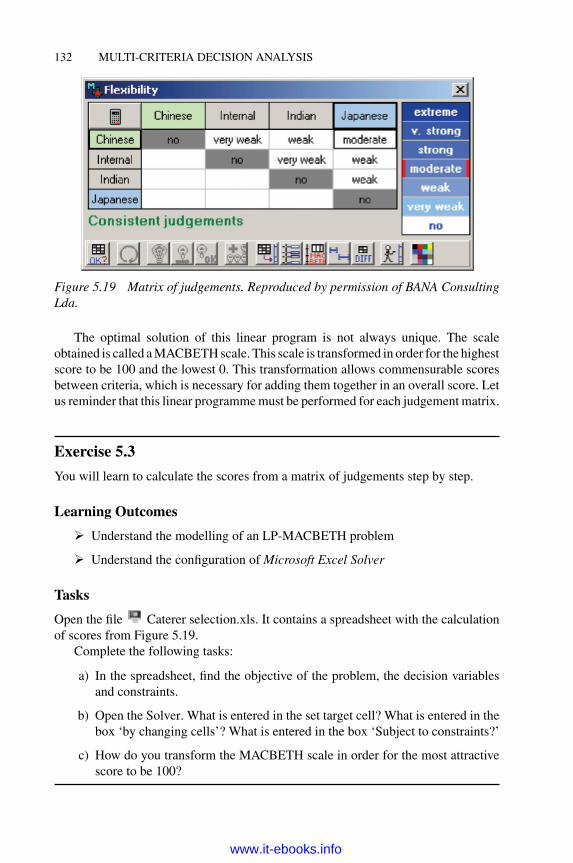
132 MULTI-CRITERIA DECISION ANALYSIS
Figure 5.19 Matrix of judgements. Reproduced by permission of BANA ConsultingLda.
The optimal solution of this linear program is not always unique. The scaleobtained is called aMACBETHscale. This scale is transformed in order for the highestscore to be 100 and the lowest 0. This transformation allows commensurable scoresbetween criteria, which is necessary for adding them together in an overall score. Letus reminder that this linear programmemust be performed for each judgement matrix.
Exercise 5.3
You will learn to calculate the scores from a matrix of judgements step by step.
Learning Outcomes
� Understand the modelling of an LP-MACBETH problem
� Understand the configuration of Microsoft Excel Solver
Tasks
Open the file Caterer selection.xls. It contains a spreadsheet with the calculationof scores from Figure 5.19.Complete the following tasks:
a) In the spreadsheet, find the objective of the problem, the decision variablesand constraints.
b) Open the Solver. What is entered in the set target cell? What is entered in thebox ‘by changing cells’? What is entered in the box ‘Subject to constraints?’
c) How do you transform the MACBETH scale in order for the most attractivescore to be 100?
www.it-ebooks.info

MACBETH 133
5.4.2 Discussion
MACBETH relies on a strongmeasurement theory foundation. This theoretical rigourraises practical issues.The judgement matrix has to be consistent enough for the calculation of the
attractiveness with a linear program. However, the decision maker might not alwaysbe consistent due to a lack of information or simply because the problem is incon-sistent by nature (e.g. a football tournament, where the highest classified team canlose against the lowest classified). In practice, the decision maker will be forced toenter judgements proposed by M-MACBETH otherwise the attractiveness cannot becalculated. The final result may not reflect the real ranking the decision maker hadin mind.Another problem of MACBETH is related to linear programming. It is well
known that several optimal solutions (i.e. rankings) can be obtained with the linearprogramming method. These different rankings can be confusing for the decisionmaker. The presence of a facilitator is therefore recommended in order to discusswhich solution would best fit their preferences.
References
Bana e Costa, C., De Corte, J.-M., and Vansnick, J.-C. (2005). On the mathematical foundationof MACBETH. In J. Figueira, S. Greco and M. Ehrogott (eds), Multiple Criteria DecisionAnalysis: State of the Art Surveys (pp. 409–437). New York: Springer-Verlag.
Bana e Costa, C., De Corte, J.-M., and Vansnick, J.-C. (2003). MACBETH. OR WorkingPaper 03.56, London School of Economics and Political Science.
Bana e Costa, C., and Vansnick, J.-C. (1999). TheMACBETH approach: Basic ideas, software,and an application. In N. Meskens and M. Roubens (eds), Advances in Decision Analy-sis, Mathematical Modelling: Theory and Applications (Vol. 4, pp. 131–157): Dordrecht:Kluwer Academic Publishers.
De Corte, J.-M. (2002). Un logiciel d’exploitation d’informations preferentielles pour l’aide ala decision. PhD thesis, University of Mons-Hainaut.
www.it-ebooks.info

Part II
OUTRANKINGAPPROACH
Multi-Criteria Decision Analysis: Methods and Software, First Edition. Alessio Ishizaka and Philippe Nemery.© 2013 John Wiley & Sons, Ltd. Published 2013 by John Wiley & Sons, Ltd.
www.it-ebooks.info

6
PROMETHEE
6.1 Introduction
This chapter describes the theory along with the practical utilization of thePROMETHEE method. You will learn how to use Smart Picker Pro, a softwarepackage that helps to express preferences amongst actions (alternatives or choices).Smart Picker Pro computes, as a main output, a partial and global ranking basedon the PROMETHEE methodology. Section 6.3 is designed for readers interested inthe methodological background of PROMETHEE, while Section 6.4 deals with theextensions of PROMETHEE in group decision and sorting problems.
The companion website provides illustrative examples in Microsoft Excel, andcase studies and examples with Smart Picker Pro.
6.2 Essential concepts of the PROMETHEE method
The acronym PROMETHEE stands for ‘Preference Ranking Organization METHodfor Enriched Evaluation’. Thus the PROMETHEE method will provide the decisionmaker with a ranking of actions (choices or alternatives) based on preference degrees.The method falls into three main steps:
1. the computation of preference degrees for every ordered pair of actions oneach criterion;
2. the computation of unicriterion flows;
3. the computation of global flows.
Based on the global flows, a ranking of the actions will be obtained as well as agraphical representation of the decision problem. Before describing these three steps
Multi-Criteria Decision Analysis: Methods and Software, First Edition. Alessio Ishizaka and Philippe Nemery.© 2013 John Wiley & Sons, Ltd. Published 2013 by John Wiley & Sons, Ltd.
www.it-ebooks.info

138 MULTI-CRITERIA DECISION ANALYSIS
more in depth, let us introduce the following case study that will be used throughoutthis chapter.
Case Study 6.1
A decision maker wants to buy a new car and is considering five different cars ofvarious types. He therefore defines four criteria:
� price (to be minimized);
� consumption (to be minimized);
� comfort (to be maximized);
� power (to be maximized).
After gathering data and testing the five cars, he evaluates their performanceson the four criteria (Table 6.1).
Table 6.1 Performance of the five cars evaluated on four criteria.
Price (£) Consumption (l/km) Comfort Power (hp)
Economic 15 000 7.5 Very Bad 50.0Sport 29 000 9.0 Bad 110.0Luxury 38 000 8.5 Very Good 90.0Touring A 24 000 8.0 Average 75.0Touring B 25 500 7.0 Average 85.0
It can be seen from Table 6.1 that no ideal car exists: no car is the best on allfour criteria. The decision maker will inevitably have to make a compromise. ThePROMETHEE method will help the decision maker in his decision process.
6.2.1 Unicriterion preference degrees
The PROMETHEE method is based on the computation of preference degrees. Apreference degree is a score (between 0 and 1) which expresses how an action ispreferred over another action, from the decision maker’s point of view.
A preference degree of 1 thus means a total or strong preference for one of theactions on the criterion considered. If there is no preference at all, then the preferencedegree is 0. On the other hand, if there is some preference but not a total preference,then the intensity will be somewhere between 0 and 1.
A decision maker might express a preference when looking at the prices of thecars of Table 6.1. The preference degree of Touring B compared to Luxury might be1 since it would mean a strong preference for the cheapest car. On the other hand, thepreference degrees between Touring A and Touring B will be relatively small, sincethey are similarly priced.
www.it-ebooks.info

PROMETHEE 139
Difference
Preference
0
1
pq Difference
Preference
0
1
s
Figure 6.1 Linear (left) and Gaussian (right) preference functions.
We use the term pairwise preference degree since the preference of action Aover action B cannot be deduced from the preference of action B over action A (norvice versa). The PROMETHEE method will help the decision maker to evaluatethese unicriterion pairwise preference degrees. For each criterion, this unicriterionpreference degree is computed through rescaling or enriching the evaluations of theactions by means of preference information.
What matters in PROMETHEE is how the decision maker perceives the differencebetween the (objective) evaluations (often measured) on every specific criterion.These pairwise comparisons are based on the difference between the evaluationsof the two actions (e.g. the difference in price between the actions). Therefore, hecan choose between two types of preference functions: the linear and the Gaussianfunction. These preference functions are shown in Figure 6.1 and Figure 6.2.
If the decision maker opts for a linear function, then the preferences will graduallyincrease as a function of the difference between the evaluations on a particularcriterion. When using the Gaussian preference function, the increase follows anexponential function.
In order to specify each preference function, one or two parameters are required.The linear preference function requires two parameters: an indifference threshold qand the preference threshold p. On the other hand, the Gaussian function requiresonly one parameter: the inflexion point s.
If the difference between the evaluations on a criterion is smaller than the indif-ference threshold, then no difference can be perceived by the decision maker betweenthese two actions (i.e. the preference degree is 0). If the difference is higher than thepreference threshold, then the preference is strong (i.e. the preference degree is 1).The preference function gives the value of the preference for differences between theindifference and preference threshold.
Figure 6.2 represents the linear preference function for particular parameters. Ifq = p = 0 (Figure 6.2(a)), then there is a strong preference for an action as soon asthere is a difference (however small the difference might be). In Figure 6.2(b) thereis no indifference zone (q=0) which signifies that every difference is consideredproportionally. Finally, in Figure 6.2(c) the preference function is given by a ‘step
www.it-ebooks.info

140 MULTI-CRITERIA DECISION ANALYSIS
0.5
Difference
Preference(a) (b) (c)
0
1
q = p = 0
Preference
0
1
pq = 0 Difference
Preference
0
1
pq
Figure 6.2 Three linear preference functions.
function’. This means that the strength of preference can only take three values: 0,0.5 or 1.
Let us consider Table 6.1 – more specifically, the price criterion which has tobe minimized. Suppose that the indifference threshold is 2000 and the preferenceis 5000. The unicriterion preference degrees of Figure 6.3 will be computed by thesoftware based on this input, but it is interesting to understand its meaning. Let ustherefore compute the unicriterion preference degrees given in Table 6.2.
All the elements of the diagonal are 0 because an action cannot be preferred toitself. Since the Sport car is more expensive than the Economic car, Sport cannot bepreferred to Economic: the preference degree (Sport, Economic) is thus necessarily0. Similarly, we have only zeros in the first column because Economic is the cheapestcar: the first column rendering how the other actions are preferred to Economic.
Since the difference between Economic and Sport is 14 000 and thus higher thanthe preference threshold p (= 5000), we show that the preference of Economic overSport is 1. Touring B is £3500 cheaper than Sport. The preference degree of TouringB on Sport can be read in Table 6.2. If you are not scared of some mathematics, thisis how the preference degree is obtained: (3500 – 2000) / (5000 – 2000) = 0.5.
1
difference
Preference
0
50002000
0.5
3500
Figure 6.3 Computation of the preference degree when the difference is 3500 andq = 2000 and p = 5000.
www.it-ebooks.info

PROMETHEE 141
Table 6.2 The unicriterion preference degrees for price with a linear function whenp = 5000 and q = 2000.
Price Economic Sport Luxury Touring A Touring B
Economic (£15 000) 0 1 1 1 1Sport (£29 000) 0 0 1 0 0Luxury (£38 000) 0 0 0 0 0Touring A (£24 000) 0 1 1 0 0Touring B (£25 500) 0 0. 5 1 0 0
If, with the same indifference and preference threshold, the decision maker hadchosen a stepwise preference function, then the difference would fall ‘in the step’(Figure 6.2). The preference would also be 0.5.
Finally, let us remark that the difference between the Touring A and Touring Bis 1500, which implies that there is no preference between those two cars from theprice point of view. The difference in price is lower than the indifference threshold.The remaining unicriterion preference degrees are given in Table 6.2.
Figure 6.4 is a graphical representation of Table 6.2. If the preference of car Aover car B is greater than 0, then there is an arrow from A to B. Thus, there is no arrowfrom Touring B to Economic since the preference of Touring B over Economic is 0.Moreover, the intensity or the size of the arrow indicates the strength of preference.This explains why the arrow between Touring B and Sport is dotted: the preferenceis only 0.5.
Moreover, from Figure 6.4 we can deduce that Economic is preferred to all theother cars since no arrow is aimed at Economic. On the other hand, Luxury is notpreferred to any other car. No preference has been expressed by the decision makerbetween the Touring A, Touring B and Sport cars: therefore there is no arrow betweenthem. Remember that this graph only relates to the price criterion.
It is worthwhile noting that although we considered numerical values in thisexample, the PROMETHEE method can deal easily with scaled values (e.g., good,
EconomicLuxury
Touring A
Sport
Touring B
Figure 6.4 Representation of the price preference degrees.
www.it-ebooks.info

142 MULTI-CRITERIA DECISION ANALYSIS
excellent, etc.). As we will see in Section 6.3.2, the verbal values need only to betranslated into numerical values.
6.2.2 Unicriterion positive, negative and net flows
It is not easy to draw conclusions from the preference degrees table (Table 6.2) or itsgraphical representation (Figure 6.4), especially when the number of actions is large.Therefore, the criterion pairwise preference degrees are summarized in the so-calledunicriterion leaving or positive flows, the entering or negative flows, and the net flows.These scores measure how an action is preferred over all other actions or how it ispreferred by all other actions.
6.2.2.1 Positive flows
The unicriterion positive flow (or leaving flow) of an action is a score between 0 and 1.It indicates how an action is preferred (according to the decision maker’s preference)over all other actions on that particular criterion. The higher this positive flow is,the more preferred the action is compared to the others (i.e. the better is the action).It is in fact an average ‘behaviour’ obtained by the average of all the preferences ofan action compared to the others (excluding the preference degree compared withitself). It is thus the normalized sum of all the row elements and always lies between0 and 1.
Referring again to our example, the positive flow of Economic is indeed 1 sincethis car is preferred over all other actions. The flows thus take into account theminimizing or maximizing aspect of the criteria. The positive flow of Luxury is 0since it is the most expensive car. The positive flow of Sport is 1/4 = 0.25 (Table 6.3).
On the left of Figure 6.5 are the initial evaluations of the cars with respect tothe price criterion. This scale is then transformed via the pairwise preferences tothe positive flows depicted on the right. Although Touring A and Touring B areindifferent (preference degrees between the two cars are 0), their positive scores areslightly different. This is due to the fact that both cars ‘behave’ differently comparedto the others cars (in particular compared to Sport). Changing the indifference andpreference thresholds changes the positive scores, and their distribution as will beillustrated further in Section 6.2.5.
Table 6.3 Positive, negative and net flows for the price criterion of Case Study 6.1.
Actions\Criterion Flows Positive Negative Net Price Flows
Economic (£15 000) 1 0 1Sport (£29 000) 0.25 0.625 –0.375Luxury (£38 000) 0 1 –1Touring A (£24 000) 0.5 0.25 0.25Touring B (£25 500) 0.375 0.25 0.125
www.it-ebooks.info

PROMETHEE 143
0
5000
10000
15000
20000
25000
30000
35000
40000
0
0.1
0.2
0.3
0.4
0.5
0.6
0.7
0.8
0.9
1
Economic (£15000)
Sport (£29000)
Luxury (£38000)
Touring A (£24000)
Touring B (£25500)
Figure 6.5 Representation of the price evaluations (on the right) and the positiveflows with q = 2000 and p = 5000.
6.2.2.2 Negative flows
Analogously, the negative flows represent an average behaviour. They measure howthe other actions are preferred to this action. The negative flow is thus obtained bytaking an average of all the preference degrees of the actions compared to that par-ticular action (excluding the preference degree compared with itself). It correspondsto the average of the entire column except for the diagonal element. This score thusalways lies between 0 and 1.
The third column of Table 6.3 gives the negative flows of all the actions for thecriterion price. Let us emphasize that this score has to be minimized since it representsthe weakness of a car compared to the other cars. Since no car is cheaper than theEconomic car, its negative flow is equal to zero.
6.2.2.3 Net flows
Finally, to take both the positive and the negative aspects into account, we use thenet flows of an action which are obtained by subtracting the negative flows from thepositive flows. These have to be maximized since they represent the balance betweenthe global strength and the global weakness of an action. The net score of an actionthus always lies between –1 and 1.
6.2.3 Global flows
In the previous section we considered only one criterion. In order to take into accountall the criteria simultaneously, the decision maker needs to provide the relative impor-tance of each criterion. For instance, the price of a car can be twice as important asthe power. On the other hand, security might be more important than price. In other
www.it-ebooks.info

144 MULTI-CRITERIA DECISION ANALYSIS
Table 6.4 Preference parameters for Case Study 6.1.
Criteria wi qi pi
Price 0.25 2000 5000Consumption 0.25 0.5 1Power 0.25 1 2Comfort 0.25 10 20
words, the decision maker specifies a weight for each criterion which permits him orher to aggregate (by means of a weighted sum) all the unicriterion positive, negativeand net flows into global positive flows, global negative flows and global net flows.These flows thus take all the criteria into account.
The relative importance of a criterion can be depicted in several ways (verbal,pairwise comparisons, etc.) but in the end it is, in any case, transformed into anumerical value associated with each criterion (i.e. the weight of the criterion). Aswe will see in Section 6.3.3, the Smart Picker Pro software offers several ways todetermine the weights of the criteria.
The global positive score indicates how an action is globally preferred to all theother actions when considering several criteria. Since the weights are normalized, theglobal positive score always lies between 0 and 1.
Analogously, the global negative score indicates how an action is preferred bythe other actions. The negative score always lies between 0 and 1 and has to beminimized.
The net flows of an action, obtained by subtracting the negative flows from thepositive flows, take into account both views (being preferred over and being preferredby all other actions).
If we consider equally weighted criteria and linear preference functions withparameters given in Table 6.4 we obtain the flows reflected in Table 6.5.
Note that we chose the following scale conversion for the comfort criterion: verybad, 1; bad, 4; average, 8 and very good, 10.
Table 6.5 Positive, negative and net flows for the cars of Case Study 6.1.
Actions Positive flows Negative flows Net flows
A1 - Economic 0.375 0.5 –0.125A2 - Sport 0.375 0.53125 –0.15625A3 - Luxury 0.34375 0.4375 –0.09375A4 - Touring A 0.375 0.28125 0.09375A5 - Touring B 0.46875 0.1875 0.28125
www.it-ebooks.info

PROMETHEE 145
6.2.3.1 The PROMETHEE I ranking
The PROMETHEE I ranking is based on the positive and the negative flows. In thisranking, there are four different scenarios when analysing the flows of two actions:
� One action has a better rank than another if its global positive and negativeflows are simultaneously better (i.e. if the global positive score is higher andthe global negative flow is lower). Considering the global positive and negativescores of Table 6.5, the Touring A car has a better rank than Luxury. This canbe easily detected from Figure 6.6, where the positive and negative scores areshown. An action should be simultaneously the first listed on the positive andnegatives axes.
� One action has a worse rank than another if both global positive and thenegative scores are worse. Touring A therefore has a worse rank than TouringB: its positive scores are lower and its negative scores are higher.
� Two actions are said to be incomparable if one action has a better globalpositive score but worse global negative score (or vice versa). Economic andLuxury are incomparable since Luxury has a lower positive score and a lowernegative score. This can be easily detected graphically as the two actions crosseach other (Figure 6.6).
� Two actions are called indifferent if they have identical positive and negativeflows.
6.2.3.2 The PROMETHEE II ranking
The PROMETHEE II ranking is based on the net flows only and leads to a completeranking of the actions (i.e. the incomparable status does not exist). The actions can
Economic
Sport
Luxury
Touring A
Touring B
Positive Flows
Negative Flows
0
0
1
1
Figure 6.6 Global positive and negative scores from Case Study 6.1.
www.it-ebooks.info

146 MULTI-CRITERIA DECISION ANALYSIS
-0.2
-0.15
-0.1
-0.05
0
0.05
0.1
0.15
0.2
0.25
0.3
0.35
Economic
Sport
Luxury
Touring A
Touring B
Figure 6.7 Global net flows from Case Study 6.1.
thus be ordered from the best to the worst: Table 6.5 gives the net scores of the carsand Figure 6.7 is the graphical representation.
To summarize the steps of the decision process, the decision maker needs todefine the criteria taken into account in his or her decision. Then all actions to beranked need to be evaluated according to those criteria. By specifying this preferenceinformation, the pairwise criterion preference degrees can be computed. From thosepreference degrees, unicriterion flows are computed. In a final step, the criterion flowsare aggregated into global flows by taking into account the relative importance ofeach criterion. We then have a ranking.
6.2.4 The Gaia plane
The Gaia plane is a two-dimensional representation of a decision problem. It containsall the aspects of the decision problem: the actions, the criteria and the decisionmaker’s preference information (thresholds and weights). We will not prolong thesuspense any further: Figure 6.8 shows the Gaia plane for the car decision problemof Case Study 6.1.
In this Gaia plane, actions are represented by bullets and criteria by arrows. Theposition of the actions gives the decision maker some idea as to their similarities: thecloser the actions, the more similar the actions. Touring A and Touring B are closeto each other in Figure 6.8. In contrast, Sport is far away from Economic. The Sportcar is thus very different from the other cars.
The similarity and non-similarity are defined by the indifference and preferencethreshold. This implies that the Gaia plane depends on the preference informationgiven by the decision maker.
Analogously, the relative position of the criteria indicates to us the correlation andanti-correlation (or conflict) of criteria. The closer the arrows, the more correlated the
www.it-ebooks.info

PROMETHEE 147
Luxury
Power
Sport
Price Economic
Touring B
Comfort
Touring AD
Consumption
Figure 6.8 Gaia plane for the car decision problem of Case Study 6.1. Reproducedby permission of Smart Picker.
criteria in the decision problem. The greater the angle between criteria, the greaterthe conflict between them. In Case Study 6.1, power conflicts with consumption:the consumption has to be minimized, the power maximized, and indeed the morepowerful a car, the more it consumes. The Gaia plane enables the visualization of theconflicting points of view.
As one can see, the lengths of the criteria are different. The length of a criterionmeasures its ‘discriminating’ or ‘differentiating’ power as a function of the data. Themore different the actions on a criterion, the longer the arrow and thus the morediscriminating the criterion. Power is represented by a long arrow since it has ahigh discriminating power, whereas consumption does not differ greatly amongst theactions. The discriminating power of a criterion depends on the chosen thresholds(the higher the indifference threshold, the less discriminating the criterion) and onthe corresponding weight.
Finally, the arrow labelled D (called the decision stick) renders the compromisesolution chosen by the decision maker, since it corresponds to his or her weight setting.The projection of the actions on this line represents their priorities. The higher theaction on the stick, the better the action. However, since this is only a two-dimensionalrepresentation, projection results in a loss of information which makes the Gaiaplane less accurate (or less representative of the decision problem). The amount ofinformation preserved (the so-called delta) depends on the data and the number ofcriteria. As a consequence of the information loss, the ranking obtained by projectionon the decision stick does not necessarily correspond to the PROMETHEE II ranking.
www.it-ebooks.info

148 MULTI-CRITERIA DECISION ANALYSIS
6.2.5 Sensitivity analysis
One of the main advantages of the Smart Picker Pro software is the ability to conduct adetailed sensitivity analysis. It is important to test the sensitivity of the ranking relativeto the input parameters. Trying different parameters (e.g. dynamically changing theweights or the indifference and preference thresholds) enables us to be aware ofthe stability or instability of the ranking. A small variation of one single parameterinducing a complete change in the ranking indicates an unstable solution. The decisionmaker needs to be aware that the conclusions drawn are only valid for this preciseset of chosen parameters and any small error or perturbation leads to a very differentsolution. If on the other hand, the ranking remains the same for a large variety ofdifferent sets of parameters, then the decision maker might be quite confident aboutthe stability of the solution.
Exercise 6.1
The following multiple-choice questions allow you to test your knowledge on thebasics of PROMETHEE. Only one answer is correct. Answers can be found on thecompanion website.
1. What does PROMETHEE stand for?
a) Positive Organization METHod with Enriched Evaluation
b) PReference Organization METHod for Enriched Evaluation
c) PROfessional METHod for Easy Evaluation
d) PROactive MEasurement THEory Evaluation
2. Which of these statements is incorrect?
a) PROMETHEE can be used in a wide range of applications
b) Every decision maker will find the same ranking
c) The PROMETHEE method requires a lot of input parameters
d) Results can be explained
3. What is the main purpose of PROMETHEE?
a) PROMETHEE prioritizes actions based on criteria and constraints
b) PROMETHEE assigns goals to actions
c) PROMETHEE ranks actions based on criteria
d) PROMETHEE assigns criteria to alternatives
4. Pairwise comparisons are based on which type of scale?
a) Ratio scale
b) Interval scale
www.it-ebooks.info

PROMETHEE 149
c) Ordinal scale
d) Nominal scale
5. How many input parameters does a decision maker need to specify for acriterion (supposing he has chosen a linear preference function)?
a) 5
b) 4
c) 3
d) 2
6.3 The Smart Picker Pro software
All the PROMETHEE computations can easily be implemented in a spreadsheet,though graphs really help the decision maker to visualize the issues and key points inthe decision. A number of user-friendly software packages have certainly contributedto the success of the PROMETHEE method. They incorporate intuitive graphicaluser interfaces, automatic calculation of preference degrees, flows, etc. One of themain advantages of the use of these software packages is the possibility to performa sensitivity analysis. This allows the user to answer questions such as ‘What if Ichange this parameter?’ which is useful in scenario planning and dealing with risk.Among those currently available are Decision Lab, D-Sight, Smart Picker Pro, andVisual Promethee.1
This section will describe the Smart Picker Pro standalone software because of itssimplicity, and because it is available as a free trial version (www.smart-picker.com)with time-unlimited use, unlike other software. The trial version is, however, restrictedto five actions and four criteria, though this is ample for gaining familiarity with itsapplication. Smart Picker Pro does not require much understanding of the method:as soon as the evaluations are entered, a ranking is available (by the use of defaultvalues which will be provided throughout this section).
However, this might not entirely reflect the decision maker’s preferences. That iswhy we suggest entering all input parameters step by step.
As an illustration, we will completely resolve Case Study 6.1 according to afictitious set of preference parameters given in Table 6.4. On the companion websitethe reader will find the basic steps of the PROMETHEE calculations in a spreadsheetas well as the Smart Picker Pro input files.
6.3.1 Data entry
The decision maker needs to first enter the decision problem before entering hispreference parameters, although actions or criteria can be deleted or added during the
1 At the time of writing, there was only a beta version of Visual Promethee.
www.it-ebooks.info

150 MULTI-CRITERIA DECISION ANALYSIS
Figure 6.9 Data entry in Smart Picker Pro. Reproduced by permission of SmartPicker.
decision process. The spreadsheet of the All Data tab (Figure 6.9) shows the actions,the criteria and the initial scores of the actions on each criterion. Each row representsan action and each column represents a criterion of the decision problem. Adding ordeleting actions or criteria can be easily done by:
� accessing the Problem menu, or
� using keyboard shortcuts (e.g., Alt+A, Alt+C, Alt+Shift+A, Alt+Shift+C),or
� placing the cell cursor on the last row or in the last column and clicking on theDown arrow (↓) or Alt + right arrow (Alt+ →).
The red value in a specific column indicates the worst evaluation for that criterionand blue the best value. This means that if a criterion is to be minimized, the lowestscore is blue and the highest score is red. The colours are reversed when maximizingcriteria.
Furthermore, the decision maker can enter numerical values as well as verbalevaluations. Sometimes, it is easier to work with a verbal scale rather than a numericalscale. For instance, it is easier to define the quality or the comfort of a car by meansof words such ‘good’, ‘average’ and ‘excellent’. As we will see, there is a method inthe software to assess how much better ‘good’ is compared to ‘average’, etc.
The PROMETHEE method permits the use of a verbal scale provided that thisscale is later translated into a numerical scale. This can be done in the Parameters tab(see Section 6.3.2).
Finally, it is worth mentioning that evaluations of all the actions are not required.In Figure 6.9 one can see that the power of the Touring A and Touring B cars areequal to ‘nan’ (i.e. not a number). This means that the user does not necessarily need
www.it-ebooks.info

PROMETHEE 151
to specify all the values. The Smart Picker Pro software will by default replace allthe missing values on one particular criterion by the mean value for this criterion.However, the user is able to change this setting by going to Data Analysis/ParametersProcessing and choosing either the median value or a desired default value.
6.3.2 Entering preference parameters
The Parameters tab by default displays the preference parameters of the first criterion(Figure 6.10). To enter the parameters of a specific criterion, the user can just pickthe criterion from the combo-box (marked 1 in Figure 6.10).
In this tab the user can specify the following preference parameters:
� the preference function – a linear function, a stepwise function or a Gaussianfunction (2 in Figure 6.10);
� the preference direction – to maximize or minimize the criterion (3 in Fig-ure 6.10);
� the values of the indifference and preference thresholds (4 in Figure 6.10).
The graph in the lower part of Figure 6.10 should help the decision maker indetermining the shape of the preference function and its thresholds. Along with the
12
34
5
6
Figure 6.10 Parameters tab in Smart Picker Pro. Reproduced by permission of SmartPicker.
www.it-ebooks.info

152 MULTI-CRITERIA DECISION ANALYSIS
Figure 6.11 Unicriterion net flows in Smart Picker Pro. Reproduced by permissionof Smart Picker.
preference function selected, all the differences between the actions on the selectedcriterion are plotted in blue on the horizontal axis. The highest difference is indicatedby D-Max (5 in Figure 6.10).
Changing the preference function and/or the preference thresholds directlychanges the shape of the preferences as depicted in Figure 6.10.
The decision maker can visualize the effect of his or her chosen preference andindifference thresholds on the unicriterion net flows/scores which are representedin (Figure 6.11), accessible via the Flow Viewer button (6 in Figure 6.10) from theParameters tab.
Note that if the decision maker does not specify any preference information,the Smart Picker Pro software will assign default values so that a ranking can stillbe computed. The default preference parameters for a criterion are: maximizing thecriterion, a linear preference function with q = p = 0 and a weight value equal to 1(which will be normalized to the other criteria).
As the perception of scale values is subjective, the user will have to define his orher scale by clicking on the Scale button in the Parameters tab. This leads him or herto the view shown in Figure 6.12. Smart Picker Pro offers several ways to translate averbal scale into a numerical scale:
� by specifying a direct numerical value for each verbal scale label.
� by ranking the verbal scale labels by their importance (i.e. specifying forinstance that very good is the best, good is the second best, etc.). The softwaregenerates a score based on this ranking.
� by pairwise comparing the labels on a 3-, 5- or 7-level scale. This enables theuser to specify for instance that very good is 3 times better than good and thatvery bad is neutral to bad.
www.it-ebooks.info

PROMETHEE 153
Figure 6.12 Entering scale definition in Smart Picker Pro. Reproduced by permissionof Smart Picker.
6.3.3 Weights
The decision maker can specify the weights in the Weights tab (Figure 6.13). He orshe can modify the value of the weights by directly dragging the weight bars up ordown or by selecting a criterion on the drop-down menu and using the slider to itsright. This can be done for a criterion relative to the others (i.e. when the weight of acriterion is increased, then the other weights will be proportionally decreased) or inabsolute terms (the values of the other weights do not change). Furthermore, SmartPicker Pro provides the user with a context-specific assistance tool for evaluating theweights (by clicking on the ‘?’button – (1 in Figure 6.13).
The decision maker can choose how he or she specifies the weights (1 in Fig-ure 6.14):
� by directly entering a value.
� by ranking the criteria according to their importance (e.g. specifying that thespace criterion is the most important). The software generates a score based onthis ranking.
� by pairwise comparing the weights on a 3-, 5- or 7-level scale. This facilitatesspecifying, for instance, that price is 3 times more important than consumptionand that power is as important as space (2 in Figure 6.14).
www.it-ebooks.info

154 MULTI-CRITERIA DECISION ANALYSIS
Figure 6.13 Weights tab in Smart Picker Pro. Reproduced by permission of SmartPicker.
Figure 6.14 Weights assistant in Smart Picker Pro. Reproduced by permission ofSmart Picker.
www.it-ebooks.info

PROMETHEE 155
Figure 6.15 Summary of the preference parameters in Smart Picker Pro. Reproducedby permission of Smart Picker.
Note here that the user can retrieve all of the preference parameters from asummary table (shown in Figure 6.15). This table can also be used to directly enterthese parameters.
6.3.4 PROMETHEE II ranking
Once the data, the preference parameters and the weights are entered, the completePROMETHEE II ranking is computed by pressing F6 or by selecting Ranking/Ranking Scores. To help the decision maker in his or her analysis, the results canbe displayed as a table (Figure 6.16) or in one of several graphical representations(accessible via the button marked 1 in Figure 6.17).
The contribution of each positive flow (stacked bar above the zero line) andnegative flow (stacked bar below the zero line) in Figure 6.18 to the net flows (thewhite dotted line and the black bullet) permit the decision maker to clearly understandthe strengths and the weaknesses of each action; and thus their rank.
For example, the Economic car has a high score due to its good performance onthe price criterion (indicated by the high price bar). However, the Economic car does
Figure 6.16 Net scores in table view in Smart Picker Pro. Reproduced by permissionof Smart Picker.
www.it-ebooks.info

156 MULTI-CRITERIA DECISION ANALYSIS
1
Figure 6.17 Graphical representation of net scores (PROMETHEE II ranking) inSmart Picker Pro. Reproduced by permission of Smart Picker.
not perform well on the comfort and power criteria. This is indicated by their negativecontribution. The Luxury car performs well only on the power criterion (only positivecontribution) and performs very badly on the price criterion.
Smart Picker Pro includes an easily understandable representation of thePROMETHEE I ranking via a triple thermometer view, where incomparability iseasily detectable. The first thermometer (on the left in Figure 6.19) indicates thescores of the negative flows, the second thermometer represents the scores of the
Figure 6.18 Criterion flows in Smart Picker Pro. Reproduced by permission of SmartPicker.
www.it-ebooks.info

PROMETHEE 157
Figure 6.19 Positive, negative and net flows in Smart Picker Pro. Reproduced bypermission of Smart Picker.
net flows, and the third thermometer shows the scores of the positive flows. Allthermometers are bounded from the worst score (bottom) to the best score (top).Therefore, the negative flow thermometer starts from 1 on the left axis and finishesat 0. A dotted line represents the score of one action on the three flows. If two linescross, there is an incomparability between the two actions.
6.3.5 Gaia plane
Smart Picker Pro provides the user with an interactive Gaia map. The projections oneach criterion and on the decision stick can be visualized easily by left-clicking on thearrows. Some information can be gained by left-clicking on the bullets (representingthe actions). Moreover, in the menu (see the toolbar in Figure 6.20), the user canchoose to display the initial performances of the actions, to see a weighted view ofthe Gaia map, etc. The user can also see the consequences of changing the thresholdsor the weights very easily: increasing the indifference threshold may lead to some
www.it-ebooks.info

158 MULTI-CRITERIA DECISION ANALYSIS
Figure 6.20 Interactive Gaia map in Smart Picker Pro. Reproduced by permissionof Smart Picker.
actions being closer (more similar). In contrast, increasing the preference thresholdor changing the preference function may lead to more spread (difference) on the Gaiamap. This step helps the decision maker to better understand the decision problem aswell as the sensitivity of the preference parameters.
6.3.6 Sensitivity analysis
As mentioned in Section 6.2.5, a variation in the values of the parameters may lead toa change in the scores and ranking. It is therefore crucial to perform some sensitivitytests in order to have an idea of the stability of the final decision. One of the mainfeatures of Smart Picker Pro is that it enables the decision maker to change all ofthe parameters dynamically while simultaneously analysing the different rankings.The user can thus directly modify all the preference parameters. On the other hand,Smart Picker Pro permits the user to change the evaluations of the actions, whilekeeping the same preference parameters. As shown in Figure 6.21, the user can
www.it-ebooks.info

PROMETHEE 159
Figure 6.21 Sensitivity analysis by changing the evaluations of the actions in SmartPicker Pro. Reproduced by permission of Smart Picker.
gradually increase/decrease the evaluation of a specific action on a chosen criterion.This permits the measurement of the required improvement (or deterioration) of thecriterion evaluation of an action in order to be higher (or lower) ranked.
Exercise 6.2
In this exercise, you will solve the car selection problem of Case Study 6.1 usingSmart Picker Pro.
Learning Outcomes
� Structure a problem in Smart Picker Pro
� Enter the preference parameters
� Understand the results
� Conduct a sensitivity analysis
Tasksa) Read the description of the Case Study 6.1, on page 138 and open Smart
Picker Pro. Choose ‘Create a new problem with the Companion’ in theopening wizard and click on the Go button.
b) Choose the left figure or Ranking actions.
www.it-ebooks.info

160 MULTI-CRITERIA DECISION ANALYSIS
c) Fill in the information about your decision problem (i.e. file name, the username, etc.). Enter the alternatives (Alternatives tab) and click on Next.
d) Enter the names of the criteria.
e) Enter the names of the actions.
f) Enter the performance of the different cars and click on Next. Specify foreach criterion if it is to be minimized or maximized.
g) Enter the weights for each criterion. If you chose equally weighted criteria,just click on Next.
h) Enter the preference parameters for each criterion as given in Figure 6.15.
i) Choose the results you want to display followed by Next. Check the resultswith the ones given in Figure 6.16–Figure 6.18.
j) Are there any incomparable actions?
k) Does the PROMETHEE II ranking change if you increase the weight of priceto 35% while maintaining the relative weight of the other criteria?
l) On which criterion does the best action perform the worst?
m) How does the decision stick move? Do the projections of the actions on thedecision stick correspond to the net flow ranking?
n) Does an increase of 10% on the power criterion change the top-two ranking?
6.4 In the black box of PROMETHEE
The PROMETHEE method has already been used successfully in a lot of cases.Behzadian et al. (2010) listed 200 papers since its conception where PROMETHEEhas been applied in environment management (47 papers), business and financialmanagement (25), hydrology and water management (28), chemistry (24), logisticsand transportation (19), manufacturing and assembly (19), energy management (17),social science (7), design (2), agriculture (2), education (2), sports (1), informationtechnology (1) and medicine (1) up to 2008. Recently, PROMETHEE has been used in
� water management (Kodika 2010; Silva et al. 2010);
� banking (Doumpos and Zopounidis, 2010);
� energy management (Ghafghazi 2010; Oberschmidt 2010);
� manufacturing and assembly (Kwak and Kim 2009; Tuzkaya 2010; VenkataRao and Patel 2010; Zhu 2010);
� logistics and transportation (Lanza and Ude 2010; Safaei Mohamadabadi 2009;Semaan 2010);
www.it-ebooks.info

PROMETHEE 161
� chemistry (Cornelissen 2010; Ni 2009);
� maritime commerce (Castillo-Manzano 2009);
� strategy (Ghazinoory 2009);
� project management (Halouani 2009);
� construction (Castillo-Manzano 2009; Frenette 2010);
� urban development (Juan 2010);
� location analysis (Luk 2010; Ishizaka et al. 2013);
� environment (Nikolic 2010; Soltanmohammadi et al. 2009; Zhang 2009);
� safety (Ramzan 2009);
� engineering (Ishizaka and Nemery 2011);
� e-commerce (Andreopoulou 2009).
The PROMETHEE method belongs to the family of outranking methods, whichmeans that the method is based on pairwise comparisons of the actions. As we willsee, the use of pairwise comparisons to infer global rankings has a direct influencewhen an action is added to or deleted from the problem (Keyser and Peeters 1996;Mareschal et al. 2008).
Denote by A = {a1,a2, . . . ,an} the set of actions to be ranked; and letF={f1,f2, . . . ,fm} be the set of criteria. As in most multi-criteria decision aid meth-ods, the set of criteria is assumed to be a coherent set of criteria as defined in Vincke(1992). Without loss of generality, we will suppose in this section that all criteriahave to be maximized. Furthermore, we will denote by fi(aj) the evaluation of actionaj on criterion fi. Let us first assume that fi(aj) is a numeric value.
In this section we will present the PROMETHEE method in a slightly differentway than in Section 6.2, where we introduced the unicriterion flows as an aggre-gation of the criterion preference degrees at a global action level, that is, from apairwise behaviour to a global behaviour. These unicriterion flows are then aggre-gated (by means of a weighted sum) to the global positive and negative flows bytaking into account the weights of the criteria. This is illustrated on the left-hand sideof Figure 6.22.
In this section we will deduce the global flows from the so-called preferencematrix. This preference matrix contains the global pairwise preference degrees,computed between all the ordered pairs of actions. The global preference degreesare deduced from the criterion preference degrees by means of the weighted sum.Based on the global preference degrees, the global flows can be easily deduced, aswe will see.
The reason for introducing this preference matrix is the information in the pairwisecomparisons. The preference matrix enables us, for instance, to detect ‘local incom-parable actions’ (incomparable if you only consider these two actions) but whichare ‘indifferent’ in the final ranking. The preference matrix contains information
www.it-ebooks.info

162 MULTI-CRITERIA DECISION ANALYSIS
Criterion preference degrees Criterion preference degrees
Global positive, negative andnet flows
Global positive, negative andnet flows
Criterion positive, negative andnet flows
Global preference degrees
Aggregation with respect to theactions
Weighted aggregationwith respect to the criteria
Aggregation with respect to theactions
Weighted aggregation with respectto the criteria
Figure 6.22 Two different ways of computing the global flows based on criterionpreference degrees.
which is lost when aggregating the pairwise preference degrees to the global flows.This computation process is represented on the right-hand side of Figure 6.22.
The two approaches are totally complementary since the first approach allowsone to render the global behaviour of an action compared to all the other actions onone particular criterion. On the other hand, the global preference degree representshow an action compares globally to one specific other action.
The outline of this section is as follows. First, we will introduce the unicriterionpreference degree. Based on this, we will define the preference degree and the prefer-ence matrix. The global flows will be directly deduced from these pairwise preferencedegrees. A sensitivity analysis will then be performed on the pairwise comparisons.
6.4.1 Unicriterion preference degrees
For each ordered pair of actions (ai,aj) of A, the unicriterion preference degree Pkij
(also noted Pk(ai , a j ) is computed and reflects how strongly action ai is preferred toaj based solely on criterion fk. Pk
ij is a number between 0 and 1, and is a function ofthe difference between the evaluations (i.e. fk(ai) – fk(aj)): the higher this difference,the stronger the unicriterion preference degree.
The preference degree is computed based on the preference functions (illustratedin Figure 6.1 and Figure 6.2). The decision maker thus has the choice between threedifferent types of preference functions. If we consider the linear preference functionwith q and p as, respectively, the indifference and preference threshold, we haveformally that
Pkij =
⎧⎪⎪⎪⎪⎨⎪⎪⎪⎪⎩
0 if fk(ai ) − fk(a j ) ≤ q[fk(ai ) − fk(a j ) − q
][p − q]
if q < fk(ai ) − fk(a j ) < p
1 if fk(ai ) − fk(a j ) ≥ p
(6.1)
www.it-ebooks.info

PROMETHEE 163
(Brans and Mareschal 2005; Brans and Vincke 1985). On the other hand, if weconsider the Gaussian preference function, where s represents the inflexion point, wehave
Pkij =
⎧⎪⎨⎪⎩
1 − exp
(−( fk(ai ) − fk(a j ))2
2s2
)if fk(ai ) − fk(a j ) ≥ 0
0 otherwise.
(6.2)
Conversely, the unicriterion preference degreePkij expresses how aj is preferred
to ai according to the decision maker. Pkij and Pk
ji are not symmetric numbers butrespect the condition 0≤ Pk
ij + Pkji ≤1.
6.4.2 Global preference degree
Having all the ordered unicriterion preference degrees, the global preference degreeπij can be computed while taking into account the weights associated to each criterion.Let wk be the weight associated to criterion fk. If the weights respect the condition∑q
k=1 wk = 1, we have (Brans et al. 1986) that
π (ai , a j ) = πij =q∑
k=1
w j · Pkij . (6.3)
The preference degree πij expresses the global preference of action ai on aj accordingto all criteria. This preference degree, which lies between 0 and 1, respects theconstraint 0 ≤ πij + πji ≤ 1. We observe that we have necessarily that ∀i : πi i = 0.
Suppose, therefore, that the preference degree reflects a ‘local’ behaviour: com-parison of one action to just one other action. The preference degree translates eitheran indifference (similar and low preference degrees between the actions, πij ≈ 0 ≈πji), an incomparability (similar and high preference degrees, πij ≈ 0.5 ≈ πji) or apreference (high difference between the preference degrees,
∣∣πij − πji
∣∣ � 0) betweentwo actions. We note here that the definitions of indifference, incomparability andpreference are not precise but left to the interpretation of the decision maker.
All the ordered pairwise comparisons are usually presented in the preferencematrix �, where the element �(i, j) represents πij.
As an illustration of this, let us consider the following numerical example:
Example 6.1 Table 6.6 represents the evaluation matrix of four actions on twocriteria. If we consider the criteria to be equally weighted, modelled with the linearpreference function where q = 0.2 and p = 0.5, we have the preference matrix givenin Table 6.7, from which we can conclude that:
� Action A1 is preferred to action A2 since we have: π12 = 1 and π21 = 0.
� Action A2 is incomparable to action A1: π32 = 0.5 and π32 = 0.5. In otherwords, actions A1 present some strength on one criterion and some weaknesseson the other criterion, compared to action A2.
www.it-ebooks.info

164 MULTI-CRITERIA DECISION ANALYSIS
Table 6.6 Numeric example.
Actions Criterion 1 Criterion 2
Action 1 (A1) 1 1Action 2 (A2) 0 0.5Action 3 (A3) 0.75 0Action 4 (A4) 1 0.1
� Actions A3 and A4 can be considered as indifferent, since the prefer-ence degrees between both actions are similar and small (π43 = 0.08 andπ34 = 0).
6.4.3 Global flows
The positive and negative flows summarize the ordered preference degrees into aunique score for each action. Let us denote by �+(ai) and �−(ai) respectively thepositive and negative flows of action ai. These can be computed as follows:
�+(ai ) =∑n
j=1 πij
n − 1, (6.4)
�−(ai ) =∑n
j=1 πji
n − 1. (6.5)
The positive flow of action ai thus represents the mean preference degree of actionai compared to all other actions. In other words, it measures the global ‘preferred’behaviour of action ai compared to the other actions. Mathematically, it correspondsto the sum of all the elements in the corresponding row divided by the number ofactions reduced by 1, as it cannot be compared to itself. The positive flow always liesbetween 0 and 1. The higher this number is, the better the action will be.
Analogously, the negative flow of action ai represents the mean preference of theother actions on action ai. In other words, it measures the global ‘being preferred’behaviour of action ai compared to the other actions. Mathematically, it corresponds
Table 6.7 Preference matrix of the problem in Table 6.6.
A1 A2 A3 A4
A1 0.0 1.0 0.58333 0.5A2 0.0 0.0 0.5 0.33333A3 0.0 0.5 0.0 0.0A4 0.0 0.5 0.08333 0.0
www.it-ebooks.info

PROMETHEE 165
Table 6.8 The global flows of the numerical example of Table 6.7.
Actions �+ �− �
Action 1 (A1) 0.69444 0 0.69444Action 2 (A2) 0.27778 0.66667 –0.38889Action 3 (A3) 0.16667 0.38889 –0.22222Action 4 (A4) 0.19444 0.27778 –0.08333
to the sum of all the elements in the corresponding column divided by the number ofactions minus 1.The negative flow also always lies between 0 and 1. The higher thisnumber is, the worse the action will be.
Finally, the net flow summarizes those two perspectives in the following way:
�(ai ) = �+(ai ) − �−(ai ). (6.6)
It is a number between –1 and 1. The higher this number is, the better the actionwill be.
All the flows of actions of Example 6.1 are given in Table 6.8 and illustratedin Figure 6.23. Observe that the scales lie between 0 and 1 for the positive andnegative flows (with an inverted orientation of the axis) and between –1 and 1 for thenet flows.
3
3
3
4 2
2
2
0 0.5 1
–1 0 1
1 0.5 01
Pos
Net
Neg
1
1
1
4
4
Figure 6.23 Graphical representation of the positive, net and negative flows ofTable 6.8. Reproduced by permission of Smart Picker.
www.it-ebooks.info

166 MULTI-CRITERIA DECISION ANALYSIS
6.4.4 PROMETHEE I and PROMETHEE II ranking
The positive and negative flows can be used to compute the PROMETHEE I ranking,which is a partial ranking, whereas the net flows can be used for the PROMETHEEII ranking, which is a complete ranking.
Let us express the relations (S+,I+) and (S−,I−) as the two complete pre-ordersinduced by the positive and negative flows (Brans and Mareschal 2005):
� The positive flow of action ai outranks the positive flow of action aj:
ai S+a j ⇔ �+(ai ) > �−(a j ).
� The positve flow of action ai and the positive flow of action aj are indifferent:
ai I+a j ⇔ �+(ai ) = �−(a j ).
� The negative flow of action ai outranks the negative flow of action aj:
ai S−a j ⇔ �−(ai ) < �−(a j ).
� The negative flow of action ai and the negative flow of action aj are indifferent:
ai I−a j ⇔ �−(ai ) = �−(a j ).
These relations permit us to define the partial PROMETHEE I ranking which is theintersection of these two pre-orders (Brans and Mareschal 2005):
� The action ai is preferred to the action aj if
ai P a j ⇔ [ai S+ a j AND ai S− a j ] OR [ai S+ a j AND
ai I− a j ] OR [ai I+ a j AND ai S− a j ].
� The action ai and the action aj are indifferent if
ai I a j ⇔ [ai I+ a j AND ai I− a j ].
� The action ai is incomaprable to the action aj if
ai J a j ⇔ [ai S+ a j AND a j S− ai ] OR [a j S+ ai AND ai S− a j ].
Here P stands for global preference, I for global indifference and J for global incom-parability.
The PROMETHEE I ranking is a partial ranking; an incomparability exists if thereis no preference or indifference relation between two actions. The partial ranking ofExample 6.1 is depicted in Figure 6.24, where ‘→’ means ‘is preferred to’. Note herethat no preference relation can be stated between A4 and A2 or between A3 and A2.
www.it-ebooks.info

PROMETHEE 167
A1
A2
A4 A3
Figure 6.24 Representation of PROMETHEE I ranking.
The PROMETHEE II ranking is a complete ranking where a preference relationexists between any pair of actions. This is due to the fact that the PROMETHEE IIranking is based solely on the net flows, which are necessarily transitive. Based onFigure 6.23, the PROMETHEE II ranking is as follows: A1 is ranked first, followedby A4, A3 and finally A2.
6.4.5 The Gaia plane
The Gaia method permits a visual representation of a decision problem and there-fore uses the unicriterion net flows computed by the PROMETHEE method. Let usconsider the matrix � containing the unicriterion net flows of all the actions of thedecision problem (Mareschal and Brans 1988):
φ =
⎛⎜⎜⎜⎜⎜⎜⎝
φ1(a1) φ2(a1) · · · φ j (a1) · · · φq (a1)φ1(a2) φ2(a2) · · · φ j (a2) · · · φq (a2)
· · · · · · · · · · · · · · · · · ·φ1(ai ) φ2(ai ) · · · φ j (ai ) · · · φq (ai )· · · · · · · · · · · · · · · · · ·
φ1(an) φ2(an) · · · φ j (an) · · · φq (an)
⎞⎟⎟⎟⎟⎟⎟⎠
(6.7)
This matrix is similar to the performance table since each row of the matrix representsan action and each column represents a criterion. However, the matrix contains somepreference information given by the decision maker since it incorporates the prefer-ence functions and their parameters. It thus measures the intra-criteria information.
In order to represent the inter-criteria information, the decision maker can usethe Gaia method (Brans and Mareschal 1994). The actions will be represented bypoints, denoted by αi with the coordinates αi: (ϕ1(ai), . . . , ϕj(ai), . . . , ϕq(ai)) inq-dimensional space. The vector αi is a line in the matrix �.
To graphically represent this matrix in two dimensions, the GAIA method usesthe statistical technique of principal component analysis (PCA). For this purpose, thevariance–covariance matrix of our decision problem, denoted by C, is first computed.This matrix can be obtained by using the relation
nC = �T · �, (6.8)
www.it-ebooks.info

168 MULTI-CRITERIA DECISION ANALYSIS
where �T denotes the transpose of �, and n is a positive integer. Then, two eigenvec-tors, denoted by u and v, are calculated such that they have the greatest eigenvaluesλ1 and λ2. These two eigenvectors are orthogonal (u⊥v) and define the best plane,called the Gaia plane, to use for the projection of the αi points while minimizing theloss of information (Brans and Mareschal 1994; Mareschal and Mertens 1990, 2003).By definition, this plane is the one that holds the maximum amount of informationafter the projection has been realized. The amount of information preserved can becalculated as follows:
δ = λ1 + λ2∑qj=1 λ j
. (6.9)
The coordinates of Ai, the projections of the αi points, on the Gaia plane will be:{ui = αT
i · u
vi = αTi · v
(6.10)
where αTi denotes the transpose of αi , αi the ith row of �.
In order to represent the intra-criteria information, each criterion fj will be pro-jected on the Gaia plane by considering each criterion axis ej as follows:
e j : (0, 0, . . . , 1, 0, . . . , 0), j = 1, 2, . . . , q (6.11)
The angle between the projections of two criteria is a measure of similarity orconflict between two criteria. The smaller the angle, the more similar the two criteria.In contrast, the angle will be greater when criteria are conflicting, given the data set.
Finally, the information on the weights chosen by the decision maker can beadded by finding the projection of the weights vector w = (w1, . . . , wq).
The vector D = (wu, wv) obtained is called a decision stick, as it represents thedecision maker’s priorities. An illustration of the Gaia plane is given in Figure 6.8.
We note here that Nemery et al. (2011) recently showed the importance of takingthe weights into account in the GAIA projections.
6.4.6 Influence of pairwise comparisons
Several authors have studied the theoretical properties of the PROMETHEE I andPROMETHEE II ranking methods (Bouyssou 1992; Bouyssou and Perny 1992;Keyser and Peeters). We now describe the major characteristics of these rankingmethods.
First, let us suppose that the preference degree π ij does not result from an aggre-gation of several criteria, but corresponds to a percentage of voters considering thataction ai is preferred or indifferent with respect to aj. We may note here that thePROMETHEE II ranking corresponds to the well-known method of Borda (Fishburn1973) where the actions are ordered according to their sums of votes (Bouyssou 1992;Bouyssou and Perny 1992). Moreover, if we suppose that ∀ai, aj ∈ A: π ij ∈ {0,1}, i.e.
www.it-ebooks.info

PROMETHEE 169
binary values, then the PROMETHEE II ranking method amounts to the Copelandranking method (Bouyssou 1992; Bouyssou and Perny 1992).
Furthermore, we can obtain the preference degrees π ij by other means as givenin previous sections. The preference degrees can be obtained while using other pref-erence functions or can even be provided directly by the decision maker (whencomparing ai to aj). Nevertheless, regardless of how these preference degrees areobtained, we may still compute the positive, negative and net flows. These rankingmethods are called ranking methods based on leaving, entering and net flows (Bouys-sou 1992; Bouyssou and Perny 1992). The PROMETHEE I and PROMETHEE IImethods are thus particular ranking methods based on flows.
The ranking methods based on net flows and on the difference of the entering andleaving flows make use of the ‘cardinal properties’ of the valued preference degrees.In fact, if we transform the preference degrees by a strict increasing transformationT(x) on the real line and such that T(0) = 0 and T(1) = 1, it may happen that theinitial flow ranking is not preserved. As a consequence, it does not seem appropriatewhen the comparisons of the valuations (preference degrees) only have an ordinalmeaning in term of credibility (Bouyssou 1992; Bouyssou and Perny 1992). ThePROMETHEE methods may only be applied if the decision maker is able to expressa preference between two actions, either on a certain criterion or on a ratio scale –and not on an ordinal scale (Keyser and Peeters 1996).
The ranking methods based on net flows and on the difference of the entering andleaving flows are said to be neutral. In particular, PROMETHEE I and PROMETHEEII do not discriminate actions in their ranking on the basis of their label or their givenname (Bouyssou 1992; Bouyssou and Perny 1992). Assume that alternatives arenumbered a1, a2, a3, . . . and then renamed (while keeping the same order) to aj, an,a3, . . . . The ranking obtained after renaming the alternatives will remain coherentwith the initial ranking.
The PROMETHEE I and PROMETHEE II ranking methods are stronglymonotonic since the rankings respond in the right direction to a modificationof the preference degrees. This property excludes, in particular, the use of anythreshold in the treatment of the valuations (Bouyssou 1992; Bouyssou and Perny1992). When two actions are compared similarly to any other action of the setA (in terms of preference degrees: π (ai , x) = π (a j , x), π (x, ai ) = π (x, ai ) andπ (ai , a j ) = π (a j , ai ),∀x ∈ A), they will be considered as globally indifferent. Thisis often called the non-discriminatory property of a ranking method. Nevertheless,it has as a drawback that a situation of indifference or incomparability between twoactions may be similarly treated in the final ranking.
When comparing actions by means of pairwise comparisons, cycles may occur:ai is preferred to aj which aj is preferred to al which is preferred to ai, etc. This is theso-called ‘Condorcet paradox’. A consequence of aggregating the comparisons intoa global complete ranking is that the order in the final ranking may not correspondto these pairwise comparisons (Mareschal et al. 2008). It may suffer from pairwiserank reversal since we may have that π (ai , a j ) > π (a j , ai ) with �(ai ) < �(a j ).
Since PROMETHEE II is not pairwise rank reversal free, it may suffer from therank reversal phenomenon: the addition to the set A or the suppression of an action of
www.it-ebooks.info

170 MULTI-CRITERIA DECISION ANALYSIS
the set A may lead to a rank reversal between two actions since the computed flowscan vary when the initial set A is altered. Some examples of pairwise rank reversalsand rank reversals are given in Keyser and Peeters (1996). Nevertheless, the rankreversal phenomenon occurs when the difference of flows between two actions is‘small’. The interested reader may find more information on situations where thereis no rank reversal in Mareschal et al. (2008), Nemery (2008) and Verly and De Smet(in press).
Exercise 6.3
In this exercise, you will learn the step-by-step calculation of the preference matrix,and then have the opportunity to compute the positive, negative and net flows.
Learning Outcomes
� Understand the calculation of the performance matrix in Microsoft Excel
� Understand the calculation of the positive, negative and net flows in MicrosoftExcel
Tasks
Open the file Car Selection.xls.Answer the following questions:
a) Describe the meaning of each calculation cell and its formula. (Only read thecomments in the red squares in the case of difficulty.)
b) Analyze Figure 6.22 and verify the complementaries and uniqueness of bothapproaches. Are there some local and global incompatibilities?
6.5 Extensions of PROMETHEE
Several extensions of the PROMETHEE method have been proposed in recentdecades. Amongst others, let us mention the extension of the PROMETHEE methodto uncertainty and imprecision (Teno and Mareschal 1998; D’Avignon and Vincke1998; Drechsler 2004; Oberschmidt 2010; Saidi Mehrabad and Anvari 2010), groupdecision support (Macharis et al. 1998; Brans and Mareschal 2005; Silva et al. 2010)and sorting problems (Araz and Ozkarahan 2007; Nemery and Lamboray 2008).In this section we briefly describe the latter two. Nemery et al. (2010) propose aunification of problem formulations with the PROMETHEE methods.
6.5.1 PROMETHEE GDSS
Sometimes decisions have to be made by a group of people rather than a single person.Rarely do all the stakeholders of the problem requiring a decision have completelyidentical perceptions and preferences with regard to the problem. Moreover, it mighthappen that not all the decision makers have the same weight of importance in the final
www.it-ebooks.info

PROMETHEE 171
decision. To tackle this situation, the group can use a group decision support system(GDSS). In what follows, we assume that the group has agreed upon a set of actionsand a set of criteria. These will not subsequently be altered by any decision maker.
The PROMETHEE GDSS method enables the tackling of a ranking probleminvolving several decision makers as follows (Macharis et al. 1998; Brans andMareschal 2005; Ishizaka and Nemery 2012). Every person acts, at first, as if hewere the only decision maker and uses the PROMETHEE II method to score andrank each action of the decision problem. In a second phase, the individual rankingsare aggregated into a group ranking. This approach is recommended when the eval-uations of the actions on the different criteria are not required to be identical for alldecision makers (i.e. no consensus about the evaluations is specified).
To aggregate the individual rankings, each individual net flow ranking will beconsidered as a criterion of the group problem. In other words, in the second phase,each decision maker will act as a criterion of the group performance matrix. Theevaluation of an action on a group criterion is equal to the net flows of that action inthe individual ranking. This is illustrated in Figure 6.25.
Each decision maker can define his own evaluations and preference parameters(preference functions, thresholds, weights, etc.) in the first step. In the second step,the weights can be equal or not depending upon whether all decision makers have thesame weight in the decision. The group of decision makers need to define whetherthe preference functions of the second phase are all identical or not.
Decision Maker A (DMA)
price power comfort security score
car A
car B
car C
Decision Maker B (DMB)
price power comfort security score DMA DMB DMC score
car A car A
car B car B
car C car C
Decision Maker C (DMC)
price power comfort security score
car A
car B
car C
Phase 1: individual ranking with PROMETHEE II
Phase 2: group ranking with PROMETHEE II
Figure 6.25 The group decision process.
www.it-ebooks.info

172 MULTI-CRITERIA DECISION ANALYSIS
The preference function will determine the role played by the difference betweenthe net flows of the actions. Small differences can be considered as negligible (useof a linear preference function with a high indifference threshold), while sometimesa small difference can be significant (use of a linear preference function with theindifference and preference threshold equal to 0).
Finally, the criterion arrows of the Gaia representation of the second phase rep-resent the individual rankings of the decision makers. Thus this means that if twoarrows are close, then the corresponding decision makers are consensual and havesimilar rankings. On the other hand, two opposite arrows indicate opposite rankingsand thus a situation of conflict between two decision makers. For detailed exampleswe refer the reader to Ishizaka and Nemery (2011, 2012).
Exercise 6.4
In this group exercise, you will be able to solve a group decision with PROMETHEEGDSS.
Prerequisites: Exercise 6.2
Learning Outcomes
� Structure a group hierarchy in Smart Picker Pro
� Understand the aggregation of individual rankings
� Understand the final group ranking
Tasks
a) Form a group of three or four people.
b) Using Smart Picker Pro, each person enters the performances of Table 6.1and his own preference parameters.
c) Collect the net flows of each decision maker and open a new problem inSmart Picker Pro. Define the problem as follows: the actions are the cars andthe criteria correspond to the different persons. The evaluation of the car foreach criterion corresponds to the net flow of the corresponding person.
d) Compute the final ranking while choosing equal weights. Discuss the finalranking. Is everybody satisfied with the outcome? Identify the persons withsimilar and opposite rankings in the Gaia plane.
6.5.2 FlowSort: A sorting or supervised classification method
In a sorting problem, the decision maker wants to assign a set of actions A = {a1,a2, . . . , an} to K predefined categories C1, . . . ,CK (Figure 6.26). The categories
www.it-ebooks.info

PROMETHEE 173
A
a1
a2 ai
R = {r1,...,rK+1}.an
aj
C1
Ch
CK
SortingMethod
Figure 6.26 The sorting process.
are predefined in the sense that the decision maker knows their exact meaning. In asorting context, there is a complete order on the categories. This means thus that thedecision maker is able to order the categories from best to worst. Category C1 is thebest category and CK the worst category.
An example of a sorting problem is the assignment of projects into two categories:the accepted or rejected projects. Several real-world decision problems have beenaddressed through sorting models, including financial decision-making problems,environmental decisions, marketing decisions, and even medical decisions (diagnosis)(Zopounidis and Doumpos, 2002).
An important requirement in a sorting problem is that the assignment of theactions is independent: the assignment of an action to a category must not depend onthe assignment of another action (i.e. the actions are not pairwise compared). Thisconstitutes a fundamental difference in dealing with the sorting problem comparedto the ranking problem. This explains why we have chosen to describe the FlowSortmethod (instead of for instance the PromSort method (Araz and Ozkarahan 2007)or the sorting method proposed by Doumpos and Zopounidis (2004) where theassignment of an action is not independent of the other assignments).
The FlowSort method (Nemery 2008; Nemery and Lamboray 2008) is a directextension of the PROMETHEE method and is based on the following idea: in orderto assign an action to a category, compare the action to the profiles by means of thePROMETHEE method and deduce its category based on its rank.
In the FlowSort method, the K categories are predefined by either limiting profilesor central profiles. In the first case, each category is defined by an upper and a lowerboundary. The category Cj is thus defined by the upper limiting profile rj (maximumvalue in order to be categorized in the Cj category) and the lower profile rj+1 (minimumvalue in order to be categorized in the Cj category) of the limiting profiles set denotedby R={r1, . . . ,rK+1}. The first category and the worst category can be defined asopen classes or as closed classes. In the former case, the two extremes categories willbe defined by an upper and lower limit respectively. In the latter case, the extreme
www.it-ebooks.info

174 MULTI-CRITERIA DECISION ANALYSIS
Figure 6.27 Limiting profiles and central profiles; open and closed categories.Reproduced by permission of Smart Picker.
categories will not be defined by these extreme limits. This can be chosen as the typeof profile in the Smart Picker Pro software, as illustrated in Figure 6.27. Definingclosed classes can be used to eliminate actions that are out of the boundaries definedby the two extreme profiles.
In the second case, the categories are defined by a central element. The categoryCj is thus defined by the central profile r∗
j .For simplicity, only the case of limiting profiles defining closed classes is pre-
sented in this chapter.So if an action ai is compared to the limiting profiles and if it is ranked between
two successive limiting profiles rh and rh+1 then it will be assigned to category Ch.
Formally, we can define the assignment rule as follows:
C (ai ) = Ch, ifφRi (rh) > φRi (ai ) ≥ φRi (rh+1) ,
where
φRi (ai ) =q∑
l=1
wl · φRil (ai ) =
q∑l=1
wl ·⎡⎣ 1
|Ri | − 1
K+1∑j=1
[Pl
(ai , r j
) − Pl(a j , ri
)]⎤⎦.
This therefore requires that the limiting profiles are always ranked with respect to thecategory they define (i.e. avoiding situations where, for instance, rh+1 has a betterrank than rh). This condition is met if a limiting profile dominates (i.e. is better onall criteria than) all the successive limiting profiles. Formally, if the criteria have tobe maximized, we need the following condition:
∀h = 1, . . . , K ; l = 1, . . . q : fl (rh) ≥ fl (rh+1) and ∃ j : f j (rh) > f j (rh+1) .
Figure 6.28 illustrates this condition, where limiting profiles rh and rh+1 definecategory Ch. In the left figure rh and rh+1 respect the condition but don’t respect it onthe right since f j (rh) < f j (rh+1).
Let us stress that the ranking method is applied on the data set consisting of oneaction to be assigned and the reference profiles, Ri = {r1, . . . , rk+1} ∪ {ai }. Thismeans thus that if n actions have to be sorted, we will perform n rankings of the setsR1, R2, . . . , Rn .
The FSGaia plane (illustrated in Figure 6.29) makes it easy to detect whetheractions (represented by circles) assigned to a same category are incomparable (e.g.,
www.it-ebooks.info

PROMETHEE 175
rh rh
rh+1
fi fj fl fi fj fl
Ch
rh+1
Figure 6.28 Limiting profiles which respect the dominance condition (left) andwhich do not respect it (right).
r4
r3
a3
a1
a2
c1
a4
a5
C3 C2 C1
r3
r1
r2
Figure 6.29 Plane representing the actions, reference profiles and criteria.
a1 and a3) or indifferent (e.g., a1 and a2). Moreover, it enables comparison of theactions in a global view of the profiles (represented by the rectangles). It is thus adescriptive approach, and is provided in Smart Picker Pro. The first application ofthe FSGaia plane in a real case study can be found in Nemery et al. (2012).
Exercise 6.5
In this exercise, you will learn how to use Smart Picker Pro in a sorting problem.
Learning Outcomes
� Structure a sorting problem in Smart Picker Pro
� Understand the steps of the FlowSort sorting method
www.it-ebooks.info
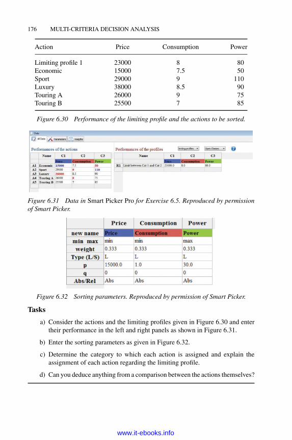
176 MULTI-CRITERIA DECISION ANALYSIS
Action Price Consumption Power
Limiting profile 1 23000 8 80Economic 15000 7.5 50Sport 29000 9 110Luxury 38000 8.5 90Touring A 26000 9 75Touring B 25500 7 85
Figure 6.30 Performance of the limiting profile and the actions to be sorted.
Figure 6.31 Data in Smart Picker Pro for Exercise 6.5. Reproduced by permissionof Smart Picker.
Figure 6.32 Sorting parameters. Reproduced by permission of Smart Picker.
Tasks
a) Consider the actions and the limiting profiles given in Figure 6.30 and entertheir performance in the left and right panels as shown in Figure 6.31.
b) Enter the sorting parameters as given in Figure 6.32.
c) Determine the category to which each action is assigned and explain theassignment of each action regarding the limiting profile.
d) Can you deduce anything from a comparison between the actions themselves?
www.it-ebooks.info
PROMETHEE 177
References
Andreopoulou, Z. K. (2009). Assessment and optimization of e-commerce websites of fishculture sector. Operational Research, 9(3), 293–309.
Araz, C. and Ozkarahan, I. (2007). Supplier evaluation and management system for strategicsourcing based on a new multicriteria sorting procedure. International Journal of ProductionEconomics, 106(2), 585–606.
Behzadian, M., Kazemzadeh, R., Albadvi, A., and Aghdasi, M. (2010). PROMETHEE: Acomprehensive literature review on methodologies and applications. European Journal ofOperational Research, 200(1), 198–215.
Bouyssou, D. (1992). Ranking methods based on valued preference relations: A characteriza-tion of the net flow method. European Journal of Operational Research, 60, 61–67.
Bouyssou, D., and Perny, P. (1992). Ranking methods for valued preference relations: Acharacterization of a method based on leaving and entering flows. European Journal ofOperational Research, 61, 186–194.
Brans, J., and Mareschal, B. (1994). The PROMCALC & GAIA decision support system formulticriteria decision aid. Decision Support Systems, 12(4.5), 297–310.
Brans, J., and Mareschal, B. (2005). Promethee methods. In J. Figeira, S. Greco, and M.Ehrgott, Multiple Criteria Decision Analysis: State of the Art Surveys. New York: Springer.
Brans, J., Mareschal, B., and Vincke, P. (1986). How to select and how to rank projects: thePromethee method. European Journal of Operational Research, 24, 228–338.
Brans, J., and Vincke, P. (1985). A preference ranking organization method: The Prometheemethod for multiple criteria decision making. Management Science, 31, 647–656.
Castillo-Manzano, J. C.-N.-V.-Q. (2009). Low-cost port competitiveness index: Implementa-tion in the Spanish port system. Marine Policy, 33(4), 591–598.
Cornelissen, T. J. (2010). Flash co-pyrolysis of biomass: The infuence of biopolymers. Journalof Analytical and Applied Pyrolysis, 85(1–2), 87–97.
D’Avignon, G., and Vincke, P. (1988). An outranking method under uncertainty. EuropeanJournal of Operational Research, 36, 311–321.
Doumpos, M., and Zopounidis, C. (2004). Developing sorting models using preference dis-aggregation analysis: An experimental investigation. European Journal of OperationalResearch, 154(3), 585–598.
Doumpos, M. and Zopounidis, C. (2010). A multicriteria decision support system for bankrating. Decision Support Systems, 50(1), 55–63.
Dreschler, M. (2004). Model-based conservation decision aiding in the presence of goalconflicts and uncertainty. Biodiversity and Conversation, 13, 141–161.
Fishburn, P. (1973). The Theory of Social Choice. Princeton, NJ: Princeton University Press.
Frenette, C. B.-Z. (2010). Multicriteria decision analysis applied to the design of light-framewood wall assemblies. Journal of Building Performance Simulation, 3(1), 33–52.
Ghafghazi, S. S. (2010). A multicriteria approach to evaluate district heating system options.Applied Energy, 87(4), 1134–1140.
Ghazinoory, S. D. (2009). A new defnition and framework for the development of a nationaltechnology strategy: The case of nanotechnology for Iran. Technological Forecasting andSocial Change, 76(6), 835–848.
Halouani, N. C. (2009). PROMETHEE-MD-2T method for project selection. European Journalof Operational Research, 195(3), 841–849.
www.it-ebooks.info

178 MULTI-CRITERIA DECISION ANALYSIS
Ishizaka, A., and Nemery, P. (2011). Selecting the best statistical distribution withPROMETHEE and GAIA. Computers & Industrial Engineering, 61(4), 958–969.
Ishizaka, A., and Nemery, P. (2012). A multi-criteria group decision framework for partnergrouping when sharing facilities. Group Decision and Negotiation, doi: 10.1007/s10726-012-9292-8, advance online.
Ishizaka, A., Nemery, P., and Lidouh, K. (2013). Location selection for the construction of acasino in the greater London region: A triple multi-criteria approach. Tourism Management,34(1), 211–220.
Juan, Y.-K. R.-L. (2010). Optimal decision making on urban renewal projects. ManagementDecision 48(2), 207–224.
Keyser, W., and Peeters, P. (1996). A note on the use of PROMETHEE multicriteria methods.European Journal of Operational Research, 89, 457–461.
Kodikara, P. P. (2010). Stakeholder preference elicitation and modelling in multi-criteria deci-sion analysis – A case study on urban water supply. European Journal of OperationalResearch, 206(1), 209–220.
Kwak, C., and Kim, C.O. (2009). A multicriteria approach to timeout collaboration protocol.International Journal of Production Research, 47(22), 6417–6432.
Lanza, G., and Ude, J. (2010). Multidimensional evaluation of value added networks. CIRPAnnals – Manufacturing Technology, 59(1), 489–492.
Luk, J. F. (2010). A conceptual framework for siting biorefineries in the Canadian Prairies.Biofuels, Bioproducts and Biorefning, 4(4), 408–422.
Macharis, C., Brans, J., and Mareschal, B. (1998). The GDSS PROMETHEE procedure:A PROMETHEE-GAIA based procedure for group decision support. Journal of DecisionSystems, 7, 283–307.
Mareschal, B., and Brans, J. (1988). Geometrical representations for MCDA. EuropeanJournal of Operational Research, 34(1), 69–77.
Mareschal, B., De Smet, Y., and Nemery, P. (2008). Rank reversal in the PROMETHEE IImethod: Some new results. Proceedings of the IEEE International Conference on IndustrialEngineering and Engeneering Management, Singapore, 959–963.
Marschal, B., and Mertens, D. (1990). Evaluation financiere par la methode Gaia: applicationau secteur bancaire. Revue de la Banque, 6/90, 317–329.
Mareschal, B., and Mertens, D. (2003). A multiple criteria decision support system for financialevaluation in the international banking sector. Journal of Decision Systems, 1, 175–189.
Nemery, P. (2008). On the use of multicriteria ranking methods in sorting problems. PhDthesis, Universite Libre de Bruxelles.
Nemery, P., Ishizaka, A., Camargo, M., and Morel, L. (2012). Enriching descriptive informa-tion in ranking and sorting problems with visualizations techniques. Journal of Modellingin Management, 7(2), 130–147.
Nemery, P., and Lamboray, C. (2008). FlowSort: a flow-based sorting method with limitingor central profiles. TOP, 16(1), 90–113.
Nemery, P., Lidouh, K., and Mareschal, B. (2011). On the use of taking weights into accountinto account in the GAIA map. International Journal of Information and Decision Sciences,3(3), 228–251.
Nemery, P., Mareschal, B., and Ishizaka, A. (2010). Unification of problem formulationwith PROMETHEE, Keynote Paper. The 52th Operational Research Society Conference(pp. 60–72). London.
www.it-ebooks.info

PROMETHEE 179
Ni, Y. L. (2009). Multi-wavelength HPLC fingerprints from complex substances: Anexploratory chemometrics study of the Cassia seed example. Analytica Chimica Acta,647(2), 149–158.
Nikolic, D. J. (2010). Multi-criteria ranking of copper concentrates according to their quality– An element of environmental management in the vicinity of copper smelting complex inBor, Serbia. Journal of Environmental Management, 91(2), 509–515.
Oberschmidt, J. G. (2010). Modified PROMETHEE approach for assessing energy technolo-gies. International Journal of Energy Sector Management, 4(2), 183–212.
Ramzan, N. N. (2009). Multicriteria decision analysis for safety and economic achievementusing PROMETHEE: A case study. Journal of Analytical and Applied Pyrolysis, 85(1–2),87–97.
Safaei Mohamadabadi, H. T. (2009). Development of a multi-criteria assessment model forranking of renewable and non-renewable transportation fuel vehicles. Energy, 34(1), 112–125.
Saidi Mehrabad, M. and Anvari, M. (2010). Provident decision making by considering dynamicand fuzzy environment for FMS evaluation. International Journal of Production Research,48(15), 4555–4584.
Semaan, N. and. (2010). A stochastic diagnostic model for subway stations. Tunnelling andUnderground Space Technology, 25(1), 32–41.
Silva, V. B. S., Morais, D. C., and Almeida, A. T. (2010). A multicriteria group decisionmodel to support watershed committees in Brazil. Water Resources Management, 24(14),4075–4091.
Soltanmohammadi, H., Osanloo, M., and Aghajani Bazzazi, A. (2009). Deriving preferenceorder of post-mining land-uses through MLSA framework: Application of an outrankingtechnique. Environmental Geology, 58(4), 877–888.
Teno, J., and Mareschal, B. (1998). An interval version of Promethee for the comparison ofbuilding products’ design with ill-defined data on environmental quality. European Journalof Operational Research, 109, 522–529.
Tuzkaya, G. G. (2010). An integrated fuzzy multicriteria decision making methodology formaterial handling equipment selection problem and an application. Expert Systems withApplications, 37(4), 2853–2863.
Venkata Rao, R. and Patel, B. K. (2010). Decision making in the manufacturing environmentusing an improved PROMETHEE method. International Journal of Production Research,48(16), 4665–4682.
Verly, C., and De Smet, Y. (in press). Some results about rank reversal instances in thePROMETHEE methods. International Journal of Multicriteria Decision Making.
Vincke, P. (1992). Multicriteria Decision Aid. Chichester: John Wiley & Sons, Ltd.
Zhang, K. K. (2009). A comparative approach for ranking contaminated sites based on therisk assessment paradigm using fuzzy PROMETHEE. Environmental Management, 44(5),952–967.
Zhu, Z. X. (2010). Optimization on tribological properties of aramid fibre and CaSO4 whiskerreinforced non-metallic friction material with analytic hierarchy process and preferenceranking organization method for enrichment evaluations. Materials & Design, 31(1), 551–555.
Zopounidis, C., and Doumpos, M. (2002). Multicriteria classification and sorting methods: Aliterature review. European Journal of Operational Research, 138, 229–246.
www.it-ebooks.info

7
ELECTRE
7.1 Introduction
This chapter describes the theory and practical uses of the ELECTRE methods. Youwill learn how to use the Electre III-IV software package which permits the (partial)ranking of options. Section 7.3 is designed for readers interested in themethodologicalbackground of the ELECTRE methods. Section 7.4 is devoted to the extensions ofELECTRE in group decision and sorting problems.The companion website provides illustrative examples withMicrosoft Excel, and
case studies and examples with the ELECTRE software package.
7.2 Essentials of the ELECTRE methods
The ELimination Et Choix Traduisant la REalite (elimination and choice expressingreality) methods, referred to as ELECTRE, belong to the outranking methods. Theyconstitute one of the main branches of this family despite their relative complexity(due to many technical parameters and a complex algorithm).The outranking methods are based on pairwise comparisons of the options. This
means that every option is compared to all other options. As we will see, this willbe computed for the user by the Electre III-IV software. Based on these pairwisecomparisons, final recommendations can be drawn.The main characteristic and advantage of the ELECTRE methods is that they
avoid compensation between criteria and any normalization process, which distortsthe original data.B. Roy, the father of the outranking methods, presented ELECTRE I for the first
time at a conference in 1965 and published the first paper on this topic in 1968(Roy 1968). This initiated a long series of improvements, research and developments
Multi-Criteria Decision Analysis: Methods and Software, First Edition. Alessio Ishizaka and Philippe Nemery.© 2013 John Wiley & Sons, Ltd. Published 2013 by John Wiley & Sons, Ltd.
www.it-ebooks.info

ELECTRE 181
Table 7.1 Overview of the different ELECTRE methods.
Decision Problem Method Software
Choice problem ELECTRE IELECTRE IvELECTRE Is
––Electre Is
Ranking problem ELECTRE IIELECTRE IIIELECTRE IV
–Electre III–Electre IVElectre III–Electre IV
Sorting problem ELECTRE-Tri-BELECTRE-Tri-C
Electre-TriIRIS
Elicitationproblem
Elicitation of the weights inELECTREElicitation for ELECTRE-Tri:� IRIS method
� other elicitation methods
SRFIRISElectre Tri Assistant
of the ELECTRE methods in order to tackle new decision problems. They can besubdivided according to the type of problem they solve (cf. Table 7.1).ELECTRE methods are relevant when facing decision problems with more than
two criteria and if at least one the following conditions is satisfied (Figueira et al.2005):
� The performances of the criteria are expressed in different units (e.g. duration,weight, price, colour, etc.) and the decision maker wants to avoid defining acommon scale, which is difficult and complex.
� The problemdoes not tolerate a compensation effect (e.g. theweak performanceof the time delay can not be compensated by good quality).
� There is a need to use indifference and preference thresholds, such that smalldifferences may be insignificant although the sum of small differences is deci-sive (e.g. we are indifferent to an additional grain of sugar in a cup of tea butnot to an additional 100 grains of sugar).
� The options are evaluated on a scale presenting an order or on a ‘weak’ intervalscale (temperature and calendar dates are examples of interval scales), whereit is difficult to compare differences (e.g. a temperature of 60◦F is 30◦F morethan 30◦F, but it cannot be said to be twice as warm as 30◦F, because intervalvariables do not have a true zero point).
The first ELECTRE method, ELECTRE I, and its variants ELECTRE Iv andELECTRE Is (cf. Table 7.1) were developed to solve choice problems. In a choice
www.it-ebooks.info

182 MULTI-CRITERIA DECISION ANALYSIS
problem the decision maker will select, amongst a given set of options, the smallestsubset containing the best options. The only difference between ELECTRE I andELECTRE Iv is the introduction of the veto concept: if an option performs badlyon a single criterion compared to another option, the option will then be consideredas outranked, irrespective of its performance on the other criteria. The novelty ofELECTRE Is is the use of pseudo-criteria. Pseudo-criteria are introduced to modelthe fact that a decision maker might not have a preference between two options ofa criterion, if the difference in their performance is smaller than the indifferencethreshold. On the other hand, it is also used to reflect a situation where the preferencemight be strong if the difference is higher than a preference threshold. Such thresholdspermit situations to be handled where data are imprecise or uncertain. Today, choiceproblems are mostly tackled with the ELECTRE Is method.ELECTRE II, ELECTRE III and ELECTRE IV (cf. Table 7.1) are ranking meth-
ods, which may lead to a partial order on a set of options (i.e. the ranking acceptsthat two options are incomparable) but without assigning a score to the alternatives.The preference order amongst the options is the output of the methods. ELECTREIII is distinguished from ELECTRE II by the use of pseudo-criteria and outrankingdegrees (instead of binary outranking relations). ELECTRE IV, on the other hand,does not require the relative importance of criteria (i.e. the weights). ELECTRE IIIis the most used ranking method in the ELECTRE family and is implemented, alongwith ELECTRE IV, in the Electre III and IV software.ELECTRE-Tri-B (more commonly known asELECTRE-Tri) andELECTRE-Tri-
C are sorting methods that enable the independent assignment of a set of options toone or several predefined categories. These methods are thus supervised classificationmethods, butwith the particularity of a preference relation amongst the categories, thatis, they can be ordered from best to worst. The difference between the two methodslies in the definition of the categories: either by limiting profiles or Boundaries (henceELECTRE-Tri-B), or by typical or Central profiles (ELECTRE-Tri-C). A detaileddescription is provided in Section 7.5.The drawback of the ELECTRE methods is that they require various (difficult)
technical parameters, which means that it is not always easy to fully understandthem. As a result, researchers have made some significant progress in the automaticelicitation of those parameters. This requires that the decision maker rank (real orfictitious) options that have a clear ranking in order to infer parameters such as theweights of the criteria, and the thresholds. These methods cannot, however, always beconsidered as a complete panacea for fixing the parameters. They may point to someof the decision maker’s inconsistencies or contradictions, which means re-evaluatingthe judgements. This might form the basis for a discussion to set the value of theparameters.The ELECTRE methods have been successfully applied in many areas such
as environmental management, agriculture and forest, energy, water management,finance, calls for tender, transportation and military (Figueira et al. 2005). In par-ticular, ELECTRE III is a well-established partial ranking method with successfulreal-world applications such as environmental and energy management (Parent andSchnabele 1988; Hokkanen and Salminen 1996; Karagiannidis and Moussiopoulos
www.it-ebooks.info

ELECTRE 183
1997; Rogers and Bruen 1998a, 1998b; Karagiannidis and Papadopoulos 2008;Figueira et al. 2005), and strategic planning (Kangas and Pykalainen 2001).The next section describes the ELECTRE III ranking method along with the
corresponding Electre III-IV software, given its success with the ELECTREmethods.Section 7.5 is devoted to the ELECTRE-Tri sorting method.
7.2.1 ELECTRE III
ELECTRE III is divided into two phases. First, the outranking relationship betweenthe options is constructed and then exploited, although most of the informationfrom the decision maker is required in the first phase: the weight of the criteria, theindifference, the preference and the veto thresholds. The meaning of those parametersis explained in this section as well as the final results of the ELECTRE III method.The intermediate steps, which require a more advanced understanding, are explainedin Section 7.4.In what follows, the term ‘alternative’ instead of ‘option’ will be used, in line
with the ELECTRE methods and software terminology. Without loss of generality,the preference directions of all criteria are taken to be increasing: in other words, allthe criteria have to be maximized.ELECTRE III makes use of outranking relations. An outranking relation, where
a outranks b (denoted by a S b),1 expresses the fact that there are sufficient argumentsto decide whether a is at least as good as b and there are no essential reasons to refutethis (Roy 1974). An outranking degree S(a,b) between a and b will be computed inorder to ‘measure’ or to ‘evaluate’ this assertion.Case Study 7.1 illustrates this concept.
Case Study 7.1
Governmental organizations and companies are often facedwith the task of recruit-ing new employees, promoting promising staff and awarding grants, etc. In today’smeeting, a committee has a travel grant to award to one of six research students.In order to evaluate the candidates, the committee has agreed on five criteria:
1. Number of years of university study (to be maximized)
2. Their professional experience expressed in years (to be maximized)
3. The requested grant amount expressed in pounds (to be minimized)
4. The evaluation of the application letter (to be maximized)
5. The potential return of the allocated grant (to be maximized).
For the last two criteria, the committee will allocate a score between 0 and 10.
1 S stands for ‘surclasse’ in French, which means ‘outranks’.
www.it-ebooks.info

184 MULTI-CRITERIA DECISION ANALYSIS
Suppose that the committee has agreed on the evaluations and the preferenceparameters. Table 7.2 suggests that there is no ideal candidate as none of theapplicants have the highest score for each of the five criteria: none of the candidatesare efficient. The committee will have to compromise.
Table 7.2 Performance table of the six applications evaluated on five criteria.
Education(years)
f1
Experience(years)
f2
Grant(× £100)
f3
Letter(score)
f4
Potentialreturn (score)
f5
Candidate 1 6 5 28 5 5Candidate 2 4 2 25 10 9Candidate 3 5 7 35 9 6Candidate 4 6 1 27 6 7Candidate 5 6 8 30 7 9Candidate 6 5 6 26 4 8
The ELECTRE III method will help the decision maker in the decision processand deduce the (final) partial order. It will compare the candidates pairwise bycalculating the outranking degrees.
The strength of the assertion a outranks b is given by the credibility or outrankingdegree S(a,b). It is a score between 0 and 1, where the closer S(a,b) is to 1, thestronger the assertion. This outranking degree S(a,b) considers two perspectives: theconcordance and the discordance of the statement that a outranks b. The concordanceand discordance are measured respectively while incorporating the decision maker’spreference on various (often conflicting) criteria. The user is required to provide theindifference and preference thresholds for calculating the concordance degree, whilethe veto threshold is needed for the discordance degree.
7.2.1.1 Concordance
A partial concordance degree ci(a,b) measures the assertion ‘a outranks b’ or ‘a isat least as good as b’ on the specific criterion fi. Table 7.2 concludes that candidate1 is as good as candidate 2 on the experience criterion. As experience has to bemaximized, this assertion is strong because the experience of candidate 1 is higherthan that of candidate 2 and as a result as good: the partial concordance degree willbe equal to 1.Consider now the opposite comparison: candidate 2 is at least as good as candidate
1 on the experience criterion (where the performances are respectively 4 versus 6).This can be true or false depending on the perception of the decision maker: oneperson can consider a difference of 2 as negligible whereas another may feel this
www.it-ebooks.info

ELECTRE 185
0
ci(a,b)
fi(b)
fi(a) fi(a)+qi fi(a)+pi
1
Figure 7.1 The partial concordance index ci(a,b).
is decisive. Therefore, the decision maker needs to specify the indifference (qi) andpreference (pi) threshold in order to measure the difference in performance.The indifference threshold indicates the largest difference between the perfor-
mances of the alternatives on the criterion considered such that they remain indifferentfor the decision maker.The preference threshold indicates the largest difference between the perfor-
mances of the alternatives such that one is preferred over the other on the consideredcriterion. Between these two thresholds, the partial concordance degree is computedon the basis of a linear interpolation, represented in Figure 7.1:
� If the performance of alternative b on fi is higher than a augmented with thepreference threshold pi, there is a strict preference for b over a. The concordancedegree stating that a is as good as b on fi is thus zero. Formally, if fi(b) is higherthan fi(a)+pi then ci(a,b) = 0.
� If the performance of b is between the performance of a augmented with theindifference threshold and the performance of a augmented with the preferencethreshold, then b is weakly preferred to a. The concordance degree is deducedby linear interpolation: if fi(b) is between fi(a)+qi and fi(a)+pi then ci(a,b) isbetween 0 and 1.
� If the performance of b is smaller than the performance of a augmented withthe indifference threshold, a and b are indifferent. The concordance degreestating that a is at least as good as b on fi is 1: if fi(b) is smaller or equal tofi(a)+qi then ci(a,b) = 1.
Table 7.3 gives some examples of the variation of the concordance index forcriterion 1 between candidate 2 and candidate 1 for different values of q1 and p1. Thereader can easily check that c1(candidate 1,candidate 2) is always 1 for any value ofq1 and p1.A global concordance degreeC(a, b) aggregates all the partial concordance indices
on the different criteria by taking into account their corresponding criteria weight.This global index is thus the weighted sum of all the partial concordance indices andmeasures how concordant the assertion ‘a is at least as good b’ is regarding all thecriteria. The Electre III-IV software computes these global concordance degrees.
www.it-ebooks.info

186 MULTI-CRITERIA DECISION ANALYSIS
Table 7.3 Some examples of c1(a,b) in Case Study 7.1for different values of q and p.
q1 p1 c1(candidate 2,candidate 1)
0 0 01 1.5 01 3 0.51 4 0.66
≥2 ≥ q1 1
7.2.1.2 Discordance
On the other hand, the partial discordance degree dj(a,b) measures the decisionmaker’s discordance with the assertion ‘a is at least as good as b’ on criterion fj. If thedecision maker, when considering criterion fj, strongly disagrees with the assertion,the discordance degree reaches its maximum value 1 and reflects the fact that fj setsits veto. This is the case if the difference in performances (i.e. fj(b) − fj(a)) is higherthan a so-called veto threshold, denoted by vi. The discordance degree has minimumvalue 0, when there is no reason to refute the assertion. As in the case of the partialconcordance degree, between these two extremes, dj(a,b) will vary linearly betweenthe preference and veto thresholds as a function of the difference fj(b) – fj(a), asshown in Figure 7.2:
� If fi(b) is higher than fi(a)+vi, the difference between b and a exceeds the vetothreshold which means a total discordance with the assertion: d(a,b) =1.
� If the performance of b is between the performance of a augmented withthe preference threshold and the performance of a augmented with the vetothreshold, b is slightly preferred to a. The concordance degree is deduced bylinear interpolation: if fi(b) is between fi(a)+pi and fi(a)+vi then, ci(a,b) isbetween 0 and 1.
0
di(a,b)
fi(b)
fi(a)+pi fi(a)+vi
1
Figure 7.2 The partial discordance degree dj(a,b).
www.it-ebooks.info
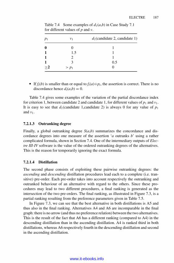
ELECTRE 187
Table 7.4 Some examples of d1(a,b) in Case Study 7.1for different values of p and v.
p1 v1 d1(candidate 2, candidate 1)
0 0 11 1.5 11 2 11 3 0.5≥2 > p1 0
� If fi(b) is smaller than or equal to fi(a)+pi, the assertion is correct. There is nodiscordance hence di(a,b) = 0.
Table 7.4 gives some examples of the variation of the partial discordance indexfor criterion 1, between candidate 2 and candidate 1, for different values of p1 and v1.It is easy to see that d1(candidate 1,candidate 2) is always 0 for any value of p1and v1.
7.2.1.3 Outranking degree
Finally, a global outranking degree S(a,b) summarizes the concordance and dis-cordance degrees into one measure of the assertion ‘a outranks b’ using a rathercomplicated formula, shown in Section 7.4. One of the intermediary outputs of Elec-tre III-IV software is the value of the ordered outranking degrees of the alternatives.This is the reason for temporarily ignoring the exact formula.
7.2.1.4 Distillation
The second phase consists of exploiting these pairwise outranking degrees: theascending and descending distillation procedures lead each to a complete (i.e. tran-sitive) pre-order. Each pre-order takes into account respectively the outranking andoutranked behaviour of an alternative with regard to the others. Since these pro-cedures may lead to two different procedures, a final ranking is generated as theintersection of the two pre-orders. The final ranking, as illustrated in Figure 7.3, is apartial ranking resulting from the preference parameters given in Table 7.5.In Figure 7.3, we can see that the best alternative in both distillations is A5 and
thus also in the final ranking. Alternatives A4 and A6 are incomparable in the finalgraph: there is no arrow (and thus no preference relation) between the two alternatives.This is the result of the fact that A6 has a different ranking (compared to A4) in thedescending distillation than in the ascending distillation. A4 is ranked third in bothdistillations, whereas A6 respectively fourth in the descending distillation and secondin the ascending distillation.
www.it-ebooks.info

188 MULTI-CRITERIA DECISION ANALYSIS
Figure 7.3 Descending and ascending distillation graphs anf the final graphobtained with the Electre III-IV software for Case Study 7.1. Reproduced by per-mission of LAMSADE.
Table 7.5 Preference parameters for Case Study 7.1.
f1 f2 f3 f4 f5
wi 0.2 0.2 0.2 0.2 0.2qi 0 0 0 0 0pi 1 1 1 1 1vi 0 0 0 0 0
Exercise 7.1
The following multiple-choice questions test your knowledge on the basics of ELEC-TRE. Only one answer is correct. Answers can be found on the companion website.
1. What does ELECTRE stand for?
a) ELimination Et Choix Traduisant la REalite
b) ELicit, Evaluate Criteria Through REferences
www.it-ebooks.info

ELECTRE 189
c) ELECitation and TRained Evaluation
d) Evidence Limitee Et Confidence Transcripte de la Realite
2. Which statement is incorrect?
a) ELECTRE can be used in a wide range of applications
b) Every decision maker will find the same ranking
c) The ELECTRE method requires a lot of input parameters
d) Results can be explained
3. What is the main purpose of ELECTRE III?
a) ELECTRE III prioritizes alternatives based on criteria and constraints
b) ELECTRE III assigns goals to alternatives
c) ELECTRE III ranks alternatives based on criteria
d) ELECTRE III sorts alternatives
4. On what scale are pairwise comparisons based?
a) Ratio scale
b) Interval scale
c) Ordinal scale
d) Nominal scale
5. How many input parameters does a decision maker need to specify for eachcriterion in ELECTRE III?
a) 5
b) 4
c) 3
d) 2
7.3 The Electre III-IV software
It is possible to implement all the ELECTRE III computation steps in a spreadsheetbut it is not a simple task. Only one software package supports the ELECTRE III andELECTRE IV methods: the Electre III-IV software. It is an old software package,which runs onWindows 3.1, 95, 98, 2000, XP and Vista. As the software is no longermaintained, it is not guaranteed to run on more recent operating systems. A freeversion is available at Lamsade at Universite Paris-Dauphine with no time expirationand with no limitation on the number of alternatives or criteria. Later in this chapter,
www.it-ebooks.info

190 MULTI-CRITERIA DECISION ANALYSIS
software supporting other ELECTRE methods (see Table 7.1) such as ELECTRE-Triis described. Electre III-IV computes the concordance matrix, discordance matrixand the different intermediate rankings. Compared to other existing software, it lacksthe functionality to enable the user to model the decision problem. It is difficult tounderstand what is happening behind the scenes and there are not many graphicalrepresentations explaining the results. Moreover, it does not perform a thoroughsensitivity analysis: the user is unable to ask questions such as ‘What if I change thisparameter?’. Nevertheless, entering the data is relatively simple and the final resultsare easy to interpret.As an illustration, Case Study 7.1 will be solved according to the set of preference
parameters set out in Table 7.5. The basic steps of the ELECTRE III calculations canbe found on the companion website in a spreadsheet format, as well as the ElectreIII-IV input files.
7.3.1 Data entry
From the menu bar, select File/New Project to create a new decision problem. Specifythe name of the owner, a small description of the decision problem and the desireddecision support method (ELECTRE III in this case).The next consecutive steps are: the definition of the criteria, the alternatives,
performance of alternatives and threshold of criteria. This is done via Edit from themenu bar.In the Edit Criteria Table window (Figure 7.4, left), click on Insert which opens
the Edit Criterion window (Figure 7.4, right). A name for the criterion, its associatedweight, direction of preference (increasing if the criterion is to be maximized ordecreasing if it is to be minimized) and optionally a code or abbreviation for thecriterion, are specified.Once the Edit Criterion window is completed, click on OK to add the criterion
to the list of criteria (displayed in the Edit Criteria Table). To add a new criterion,click on the Insert button again, which opens a blank Edit Criterion window. To avoidgoing back to Edit Criteria Table, the Auto Insert Mode in the Edit Criteria Table
Figure 7.4 The Edit Criteria Table (left) and Edit Criterion (right) windows. Repro-duced by permission of LAMSADE.
www.it-ebooks.info

ELECTRE 191
Figure 7.5 The Edit Alternatives Table (left) and Edit Alternative (right) windows.Reproduced by permission of LAMSADE.
window can be activated: the Edit Criterion window will continuously appear afterclicking OK until Cancel is selected. In order to modify the parameters of an alreadydefined criterion, double-click on the name of the criterion from the list.The definition of the alternatives is done in an analogous way: from the Edit
Alternatives Table (via Edit/Alternatives) open the Edit Alternative window (seeFigure 7.5).Once the criteria and alternatives have been defined, enter the performance of the
alternatives in the Edit Performances Table dialogue box (see Figure 7.6) by selectingEdit/Performances from the menu bar. We remark that only numerical values can beentered in the software.At this stage, the criteria, alternatives and their performance have been entered.
Following this, the decision maker needs to introduce the preference settings.
7.3.2 Entering preference parameters
The user needs to define the preference parameters for each criterion via the EditThresholds Table (see Figure 7.7). Analogously, the user can change the settings by
Figure 7.6 The Edit Performances Table. Reproduced by permission of LAMSADE.
www.it-ebooks.info

192 MULTI-CRITERIA DECISION ANALYSIS
Figure 7.7 Input boxes for preference information. Reproduced by permission ofLAMSADE.
choosing a criterion in the Edit Thresholds Table window (Figure 7.7, left), whichleads to the Edit Thresholds window (Figure 7.7, right).Various parameters are required. The user has to define the indifference and
preference threshold for each criterion. The veto threshold is optional (by checkingthe Disable Veto box).The ELECTRE III preference thresholds can be constant values or proportionate
to the performance of the alternative. If the user wants to use a fixed threshold,the α-coefficient must be equal to 0. The β-coefficient takes the value of the fixedthreshold. The Mode of Definition does not play any part in this situation.In Case Study 7.1, the indifference and preference thresholds for the criterion f5
were set to 0 and 1, respectively (see Table 7.5). These parameters are entered intoElectre III-IV (see Figure 7.7, right):
� α-indifference coefficient = 0,� β-indifference coefficient = 0,� α-preference coefficient = 0;� β-preference coefficient = 1.
Moreover, we need to disable the veto.
7.3.2.1 Advanced settings
Let us suppose that with regard to the potential return criterion of Case Study 7.1, thedecision maker considers that two alternatives are indifferent if their score differenceis less than 10%. In this case, the indifference threshold is not absolute, but relativeto the performance of the alternatives.This relative proportion is introduced via the coefficient α of the indifference and
preference thresholds in the software. The user needs to specify which performancethe proportion is taken from: either 10% from the highest performance or 10% fromthe lowest one. This can be specified by the ‘mode of definition’ (see Figure 7.7, left):if the direct mode is chosen, the worst performance between the two will be used tocompute the relative threshold. The term ‘worst’ means ‘the least preferred’, whichmight be the lowest value for criteria to be maximized or highest for criteria to beminimized. If the mode of definition is ‘inverse’, the best performance is chosen.
www.it-ebooks.info
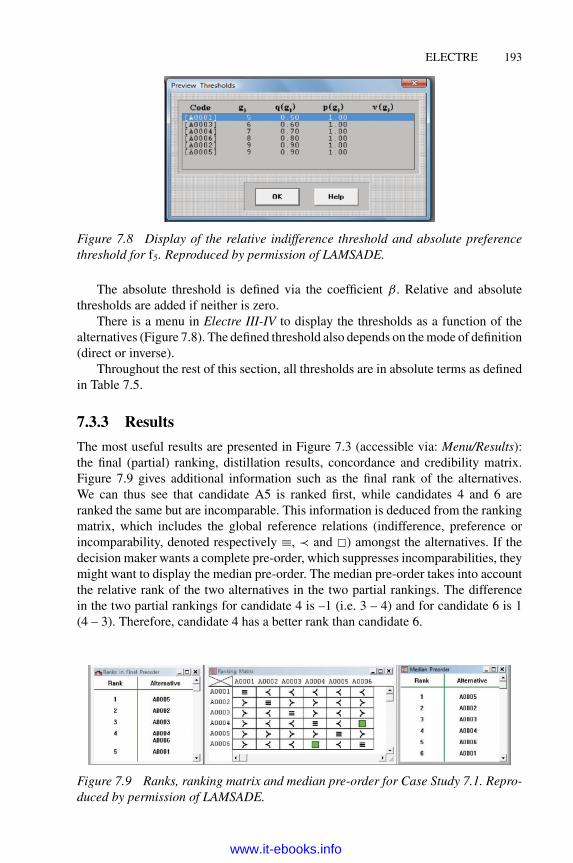
ELECTRE 193
Figure 7.8 Display of the relative indifference threshold and absolute preferencethreshold for f5. Reproduced by permission of LAMSADE.
The absolute threshold is defined via the coefficient β. Relative and absolutethresholds are added if neither is zero.There is a menu in Electre III-IV to display the thresholds as a function of the
alternatives (Figure 7.8). The defined threshold also depends on themode of definition(direct or inverse).Throughout the rest of this section, all thresholds are in absolute terms as defined
in Table 7.5.
7.3.3 Results
The most useful results are presented in Figure 7.3 (accessible via: Menu/Results):the final (partial) ranking, distillation results, concordance and credibility matrix.Figure 7.9 gives additional information such as the final rank of the alternatives.We can thus see that candidate A5 is ranked first, while candidates 4 and 6 areranked the same but are incomparable. This information is deduced from the rankingmatrix, which includes the global reference relations (indifference, preference orincomparability, denoted respectively ≡, ≺ and �) amongst the alternatives. If thedecision maker wants a complete pre-order, which suppresses incomparabilities, theymight want to display the median pre-order. The median pre-order takes into accountthe relative rank of the two alternatives in the two partial rankings. The differencein the two partial rankings for candidate 4 is –1 (i.e. 3 – 4) and for candidate 6 is 1(4 – 3). Therefore, candidate 4 has a better rank than candidate 6.
Figure 7.9 Ranks, ranking matrix and median pre-order for Case Study 7.1. Repro-duced by permission of LAMSADE.
www.it-ebooks.info

194 MULTI-CRITERIA DECISION ANALYSIS
Exercise 7.2
In this exercise, you will solve the problem set out in Case Study 7.1 with ElectreIII-IV.
Learning Outcomes
� Structure a problem in Electre III-IV
� Enter the preference parameters
� Understand the results
Consider Case Study 7.1 where the performance of the alternatives is given inTable 7.2 and the preference parameters in Table 7.5. Enter the data in Electre III-IVand cross-reference your results with those set out in Figure 7.3 and Figure 7.9.
Tasksa) Read the description of Case Study 7.1 on page 183 and open the Electre
III-IV software. Choose New Project from the File menu; specify the nameof the owner and choose ELECTRE III as the ranking method.
b) From Edit select Criteria, which displays the Edit Criteria Table where anew criterion can be inserted. For each criterion specify its name, weight anddirection of preference.
c) FromEdit selectAlternatives,which displays the Edit Alternative Tablewherenew alternatives can be inserted. For each alternative specify the name andcode name.
d) From Edit select Performances, which presents the Edit Performances Tablewhere the performance of the alternatives can be edited.
e) From Edit select Thresholds, which displays the Edit Threshold Table wherethe preference parameters of the criteria can be edited.
g) Check the results against those in Figure 7.3 and Figure 7.9.
g) Check that the concordance matrix corresponds to Table 7.6.
h) Are there any incomparable actions?
7.4 In the black box of ELECTRE III
7.4.1 Outranking relations
ELECTRE III makes use of outranking relations. An outranking relation on a set A isa binary relation: a collection of ordered pairs of elements ofA and thus a subset of theCartesian product A × A (where A × A = {(a,b)|a∈A and b∈A}; this means that it is
www.it-ebooks.info

ELECTRE 195
1. For each criterion fi of the set F:
2. Aggregation of the concordance and discordance degrees:
partial discordance degree:di(a,b)
global concordance degree:C(a,b)
global discordance degree:D(a,b)
partial concordance degree:ci(a,b)
Outranking degreeS(a,b)
3. Calculation of the outranking degree or credibility index
Figure 7.10 Steps in the calculation of the outranking degree S(a,b).
the set of all possible ordered pairs). According to (Roy 1974), an outranking relationis such that for two elements a and b of A, a outranks b (written a S b), if, given whatis known about the decision maker’s preferences, the quality of the valuations of thealternatives and the nature of the problem, there are enough arguments to decide thata is at least as good as b, where there is no essential reason to refute this statement.An outranking degree S(a,b) between a and b will be computed to ‘measure’ or
‘evaluate’ this assertion. The score will be between 0 and 1: the stronger the assertion,the closer S(a,b) to 1. The outranking relation is a non-symmetric relation:∃a, b ∈A : S(a, b) �= S(b, a).The outranking degree is calculated in three steps as shown in Figure 7.10:
1. The partial concordance and partial discordance degrees are computed for eachcriterion of the set F.
2. The criteria are aggregated to the global concordance and global discordancedegree.
3. The aggregation of the concordance and discordance degree leads to the out-ranking degree or credibility index.
7.4.2 Partial concordance degree
For each criterion fj from F the assertion ‘b is at least as good as a’ or ‘b outranks a’is measured by the partial concordance index noted cj(b,a). This degree is obtained
www.it-ebooks.info

196 MULTI-CRITERIA DECISION ANALYSIS
as follows (Roy and Bouyssou 1993):
c j (b, a) =
⎧⎪⎪⎪⎪⎨⎪⎪⎪⎪⎩
1 if f j (b)+ p j < f j (a)f j (b)+ p j − f j (a)
p j − q jif f j (b)+ q j < f j (a) < f j (b)+ p j
0 otherwise,(7.1)
where qj, pj (satisfying pj > qj) represent respectively the indifference and preferencethresholds as illustrated in Figure 7.1.These thresholds may be absolute or dependent (i.e. relative) on the performances
of a or b: p j = p j ( f j (b)) and q j = q j ( f j (b)). The stronger the confidence of thedecision maker with the outranking assertion, the higher the concordance index. Itsvalue is always between 0 and 1. A concordance degree of 0 means that b does notoutrank a. A score of 1means that b is as least as good as a (on this particular criterion).
7.4.3 Global concordance degree
The global concordance degree C(a, b) aggregates all the partial concordance indiceson the different criteria by taking into account their corresponding weight, denotedby wj for all fj with j = 1, . . . q . It is the weighted sum of all the partial concordanceindices, which measures how concordant the assertion ‘a is at least as good b’ is,regarding all the criteria. We have
C(b, a) =∑
j=1,...,qw j · c j (b, a). (7.2)
We remark that the weight of the criteria cannot be considered as substitution ratesas in compensatory methods such as AHP (Chapter 2), MAUT (Chapter 4) andMACBETH (Chapter 5) (Figueira et al. 2005). The weights depend neither on therange nor the scale of the criteria (Figueira et al. 2005).To illustrate, consider the performancematrix of Case Study 7.1 given in Table 7.2
and the preference parameters given in Table 7.5. This leads to the concordancematrixin Table 7.6.
7.4.4 Partial discordance degree
For each criterion fj from F, the measure of the discordance with the assertion ‘b isat least as good as a’ is given by the partial discordance index dj(a,b). This index iscalculated as follows:
d j (b, a) =
⎧⎪⎪⎪⎪⎨⎪⎪⎪⎪⎩
1 if f j (b)+ v j < f j (a)0 if f j (a) < f j (b)+ p jf j (a)− p j − f j (b)
v j − p jotherwise, (7.3)
www.it-ebooks.info
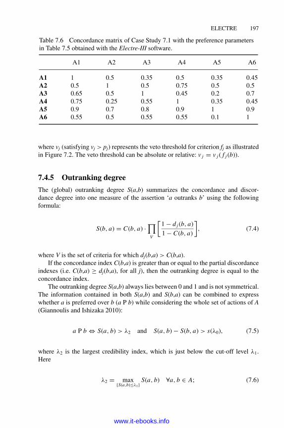
ELECTRE 197
Table 7.6 Concordance matrix of Case Study 7.1 with the preference parametersin Table 7.5 obtained with the Electre-III software.
A1 A2 A3 A4 A5 A6
A1 1 0.5 0.35 0.5 0.35 0.45A2 0.5 1 0.5 0.75 0.5 0.5A3 0.65 0.5 1 0.45 0.2 0.7A4 0.75 0.25 0.55 1 0.35 0.45A5 0.9 0.7 0.8 0.9 1 0.9A6 0.55 0.5 0.55 0.55 0.1 1
where vj (satisfying vj > pj) represents the veto threshold for criterion fj as illustratedin Figure 7.2. The veto threshold can be absolute or relative: v j = v j ( f j (b)).
7.4.5 Outranking degree
The (global) outranking degree S(a,b) summarizes the concordance and discor-dance degree into one measure of the assertion ‘a outranks b’ using the followingformula:
S(b, a) = C(b, a) ·∏
V
[1− d j (b, a)
1− C(b, a)
], (7.4)
where V is the set of criteria for which dj(b,a) > C(b,a).If the concordance index C(b,a) is greater than or equal to the partial discordance
indexes (i.e. C(b,a) ≥ dj(b,a), for all j), then the outranking degree is equal to theconcordance index.The outranking degree S(a,b) always lies between 0 and 1 and is not symmetrical.
The information contained in both S(a,b) and S(b,a) can be combined to expresswhether a is preferred over b (a P b) while considering the whole set of actions of A(Giannoulis and Ishizaka 2010):
a P b ⇔ S(a, b) > λ2 and S(a, b)− S(b, a) > s(λ0), (7.5)
where λ2 is the largest credibility index, which is just below the cut-off level λ1.Here
λ2 = max{S(a,b)≤λ1}
S(a, b) ∀a, b ∈ A; (7.6)
www.it-ebooks.info

198 MULTI-CRITERIA DECISION ANALYSIS
λ1 is the cut-off level
λ1 = λ0 − s(λ0); (7.7)
λ0 is the highest degree of credibility in the credibility matrix,
λ0 = maxa,b∈A
S(a, b); (7.8)
and s(λ0) is the discrimination threshold,
s(λ0) = α + βλ0. (7.9)
In this obscure formula, α and β are technical parameters that Roy and Bouyssou(1993) suggest setting to α = –0.15 and β = 0.3.It is worth noting that the preference relation between two actions, in ELECTRE
III, is dependent on the outranking degrees between the other actions given thedefinitions of λ2 and λ0. This is not the case with the preference relation, defined inELECTRE-Tri (Section 7.5).To illustrate, consider Case Study 7.1, where the preference relations of the
alternatives are computed based on the concordance matrix given in Table 7.6. Theparameters are given in Table 7.7. Based on these parameter values, the followingpreference relation between two alternatives of A exist:
a P b ⇔ S(a, b) > 0.8 and S(a, b)− S(b, a) > 0.15. (7.10)
Equation (7.11) leads to the following conclusions: alternative A1 is preferred to noother alternative as its outranking relation to the other alternatives is always lowerthan 0.8. Alternative A5 is the only alternative preferred over A1: S(A5,A1) = 0.9 >
0.8 and S(A5,A1) – S(A1,A5) = 0.55 > 0.15 and as a result A5 � A1.Considering two outranking degrees S(a,b) and S(c,d) with S(a,b) > S(c,d), it is
tempting to say that the assertion ‘a outranks b’ is more credible (or more likely) than
Table 7.7 Values of the parametersfor Case Study 7.1.
Parameters Values
λ0 1α, β α=–0.15 and β=0.3s(λ0) 0.15λ1 0.85λ2 0.8
www.it-ebooks.info

ELECTRE 199
the assertion ‘c outranks d’. Due to the arbitrary nature of the computation of theseindices, this should be avoided (Tervoren et al. 2004). However, if λ ∈ [0,1] and if[S(a,b) = λ and S(c,d) = λ – η with η > s(λ0)], then we can say that a S b is strictlymore credible than c S d.
7.4.6 Partial ranking: Exploitation of the outranking relations
The second phase consists of exploiting the outranking degrees by the ascendingand descending procedures, which give two complete (i.e. transitive) pre-orders O1and O2. The final ELECTRE III partial pre-order, O, is obtained by calculating theintersection of O1 and O2.The distillation procedures are based on the qualification of the alternatives. The
qualification score of an alternative is a score which characterizes its global behaviourwith regard to the other alternatives. Each time one action is preferred to another, thescore is incremented by 1 (strength), whereas if it is preferred by another, this scoreis reduced by 1 (weakness). The qualification of an alternative is thus the balance ofits strengths and weaknesses.For instance, in Case Study 7.1, the strength of candidate 1 is 0 (candidate 1 is not
preferred to any other alternative) and its weakness is 1 (one other candidate (can-didate 5) is preferred to candidate 1). Therefore, the qualification of candidate 1will be –1.The descending distillation procedure leading to the complete pre-order O1 can
be explained as follows:
� We start with the complete set of alternatives. From this set, the alternative(s)fromAwith the highest qualification is extracted. This constitutes the first group(denoted byC1). Thismeans that it is not possible to decide between the remain-ing alternatives in the subset, and therefore they are declared indifferent andbelong to C1.
� From the remaining set of alternatives (i.e. A\C1), the best alternative isagain extracted to obtain the second group C2. On the successive distilla-tions, the cut-off level λ1 (defined in (7.8)) is progressively reduced, whichmakes the condition weaker and easier for an alternative to be preferred overanother.
� This procedure is repeated until A has been distilled completely (i.e. all alter-natives of A belong to a subgroup).
The complete descending pre-order corresponds to the order C1, C2, etc. Figure 7.11illustrates the descending distillation procedure, while Figure 7.3 represents thedescending pre-order of Case Study 7.1.The ascending distillation procedure is comparable in some respects; however,
instead of starting with the best subset, it starts with the worst.
www.it-ebooks.info

200 MULTI-CRITERIA DECISION ANALYSIS
a1
a1
a1
a2
a2
a3
a3a6
a6
Step 1 Step 2 ...
a6
a5
a5
C1
C2
A
A\C1
A\(C1 C2)
a4
a4
a4
a2 a3
Figure 7.11 The descending distillation procedure.
The final partial pre-order O is defined as the intersection of O1 and O2. Theglobal relations are defined as follows:
� a is globally better than b, written a � b, if and only if:
◦ a is better than b in O1 and in O2, or
◦ a is indifferent with respect to b in O1 but better than b in O2, or
◦ a is better than b in O2 and indifferent with respect to b in O2.
� a and b are globally indifferent, written a ≡ b, if and only if a and b areindifferent in O1 and O2.
� a is globally incomparable to b, written a � b, if and only if:
◦ a is better than b in O1 but b is better than a in O2,
◦ b is better than a in O1 but a is better than b in O2.
� a is globally worse than b, written a ≺ b, if and only if:
◦ b is better than a in O1 and in O2, or
◦ a is indifferent with respect to to b in O1 but b is better than a in O2, or
◦ b is better than a in O2 and indifferent with respect to a in O2.
Example 7.1 Consider the following example, where four alternatives are to beranked with the ELECTRE III partial rankingmethod according to two criteria. Thesecriteria are to be maximized; suppose that they are true criteria (i.e. for all j = 1,2: qj = pj = 0 and with vj = 0). The performance matrix of A is given in Table 7.8.The binary relations (based on the values of the credibility matrix S) are given inTable 7.10 and represented in Figure 7.12 when fixing λ > 0.5.
www.it-ebooks.info

ELECTRE 201
Table 7.8 The performance matrixof the alternatives in Example 7.1.
f1 f2
a1 1 1a2 0 0.5a3 0.5 0a4 0 0
a1a4
a2
a3
Figure 7.12 Outranking graph of A.
Table 7.9 The outranking degrees for Example 7.1.
S a1 a2 a3 a4
a1 1 1 1 1a2 0 1 0.5 1a3 0 0.5 1 1a4 0 0 0 1
Based on the outranking matrix given in Table 7.9, the outranking graph givenin Figure 7.12 can be drawn, where an arrow between two alternatives represents a(binary) preference relation; thus a3 and a2 are incomparable.The ascending and descending distillation procedures lead to the complete ranking
represented in Figure 7.13 with the ranking relations given in Table 7.10. The resultswere acquired from Electre III-IV.
O = O1 = O2 :
a1 a4a2 a3,
Figure 7.13 The partial pre-order for Example 7.1 obtained with ELECTRE III.
From Figure 7.13, ELECTRE III leads to a complete pre-order, although a moreintuitive partial ranking could be expected on the basis of the outranking graph inFigure 7.12. If only the transitive outranking relations are represented, the partial
www.it-ebooks.info

202 MULTI-CRITERIA DECISION ANALYSIS
Table 7.10 The binary relation betweenthe alternatives in the global ranking O.
S a1 a2 a3 a4
a1 ≡ � � �a2 ≺ ≡ ≡ �a3 ≺ ≡ ≡ �a4 ≺ ≺ ≺ ≡
pre-order given in Figure 7.14 (what we will call the reduced outranking graph) isobtained. The main difference lies in the incomparability between a2 and a3 beingpreserved.A potential drawback of the ELECTRE III method is that it cannot always clearly
differentiate between indifference and incomparability between two alternatives inthe final ranking (Roy and Bouyssou, 1993, p. 423). As one might notice, the prefer-ence relations given in Table 7.10 are based on a ‘global’ level. However, based onthese outranking degrees and a cut-off level λ defined by the decision maker, fourpossible pairwise (local) comparisons can be defined when comparing alternative ato alternative b:
� a P+ b: a is preferred to b if and only if S(a, b) ≥ λ and S(b, a) < λ, that is,we have that a is at least as good as b but b is not at least as good as a.
� a P− b: b is preferred to a if and only if S(a, b) < λ and S(b, a) ≥ λ, that is,we have that a is not at least as good as b but b is at least as good as a.
� a I b: a and b are indifferent if and only if S(a, b) ≥ λ and S(b, a) ≥ λ, thatis, we have that a is at least as good as b and b is at least as good as a.
� a R b: a and b are incomparable if and only if S(a, b) < λ and S(b, a) < λ,that is, we have that a is not at least as good as b but neither is b compared to a.
If we define a value higher than 0.5 for the cut-off level λ, we obtain the pairwisepreference relations given in Table 7.11.
a1a4
a2
a3
Figure 7.14 The partial pre-order of the set of alternativesA obtained by ‘reducing’the outranking graph.
www.it-ebooks.info

ELECTRE 203
Table 7.11 The pairwise preference relationsbetween the alternatives.
a1 a2 a3 a4
a1 I P+ P+ P+
a2 P− I R P+
a3 P− R I P+
a4 P− P− P− I
As we can see from Table 7.11, the alternatives a2 and a3 are (locally) incom-parable but are considered as indifferent in the global ranking O (see Table 7.10).The decision maker can nevertheless accept this as a2 and a3 behave similarly withrespect to the alternatives a1 and a4. An analogous result would be obtained withPROMETHEE. This is a direct consequence of the aggregation of the pairwisecomparisons. To avoid this situation, a modified version of ELECTRE III has beenproposed and can be found in Roy and Bouyssou (1993).
7.4.7 Some properties
When comparing alternatives by means of pairwise outranking degrees, cycles mayoccur, for example, ai outranks aj outranks ak outranks ai. This is the ‘Condorcetparadox’. The consequence of aggregating the comparisons into a global completeranking is that the order in the final rankingmay not correspond to these pairwise com-parisons (Mareschal et al. 2008). It may suffer from pairwise rank reversal since a S bwith b having a better rank in the final ranking than a. InO1 of Case Study 7.1, noticethat a6 has a lower rank than a4 (see Figure 7.14) even though S(a4, a6) < S(a6, a4).A consequence of pairwise rank reversal, as described byMareschal et al. (2008),
is that the addition or the suppression of an alternative to set A may lead to a rankreversal phenomenon in the final ranking. The pre-ordersO1 andO2 can be modified.Wand and Triantaphyllou (2006) conducted some computational experiments on ran-domly generated and real-life decision problems to test the rank reversal phenomenonwith the ELECTRE III method. They observed that the rates of ranking irregularitieswere significant in both the simulated and real-life decision problems.ELECTRE III is neutral to the name or label given to the alternatives, as it does
not discriminate alternatives in their ranking on the basis of their label or their givenname (Bouyssou and Perny 1992; Bouyssou 1992). Assume that alternatives arenumbered a1, a2, a3, . . . ., and then renamed (while keeping the same order) to aj, an,a3, . . . . The ranking obtained after renaming the alternatives will remain coherentwith the initial ranking.When two alternatives, a and b, are compared similarly to any other alternative
of set A (i.e. ∀x ∈ A: S(a, x) = S(b, x); S(x, a) = S(x, b) and S(a, b) = S(b, a)), theywill be considered globally indifferent. This is often called the non-discriminatoryproperty of a ranking method.
www.it-ebooks.info

204 MULTI-CRITERIA DECISION ANALYSIS
Finally, Gabrel (1990) and Perny (1992) have pointed out that ELECTRE III doesnot fulfill the property of monotonicity since the rankings do not respond ‘in the rightdirection’ to a modification of performances of the alternatives: the amelioration ofthe performances of an alternative may lead to deterioration in its final ranking.
Exercise 7.3
You will learn the calculation of the outranking matrix step by step, and then havethe opportunity to compute the rank of the alternatives based on the distillationprocedures.
Learning Outcomes
� Understand the calculation of the outranking matrix inMicrosoft Excel
� Understand the calculation of the ascending and descending distillation pro-cedures
� Understand the calculation of the final ranking
Tasks
Open the file Grant.xls. The spreadsheet contains the steps of the ELECTRE IIIprocedure. Answer the following questions:
a) Describe the meaning of each calculation cell and its formula. (Read thecomments in the red square in case of difficulty.)
b) The spreadsheets are incomplete because they calculate only one local alter-native. Complete them in order to calculate the other local alternatives.
7.5 ELECTRE-Tri
7.5.1 Introduction
ELECTRE-Tri is a multi-criteria sorting method used for the assignment of a set ofalternatives A into K completely ordered categories C1, . . . ,CK where category C1 isthe best category and CK the worst. For example, the prioritization of projects, whichare categorized as low, medium or high priority.In ELECTRE-Tri, the categories can be defined either by limiting profiles (or
boundaries (Yu 1992)) or by central profiles (or centroids (Dias et al. 2010)). In thefirst case, the method is named ELECTRE-Tri-B and in the second ELECTRE-Tri-C. In this section, ELECTRE-Tri-B, which has been named ELECTRE-Tri, will bedescribed.A limiting profile rh is the upper reference profile for category Ch and the lower
reference profile for category Ch–1. The best profile will be denoted by r1 and the
www.it-ebooks.info

ELECTRE 205
rh rh
Ch
rh+1 rh+1
fi fj fl fi fj fl
Figure 7.15 Limiting profiles respecting (left) and infringing (right) the dominancecondition.
worst rK+1 . This convention has been chosen because the best category is ranked 1and the worst has is ranked K.Since the limiting profiles define ordered categories, they need to respect the
condition of dominance: a limiting profile dominates, written �D , all the successivelimiting profiles of worse categories. Formally, if all the criteria fl (l = 1, . . . , q) areto be maximized, the following condition has to be satisfied:
∀h = 1, . . . , K ; rh �D rh+1 ⇔ ∀l = 1, . . . , q : fl(rh) ≥ fl (rh+1)and ∃ j : f j (rh) > f j (rh+1).
(7.11)
This condition implies that the performance of the upper limit of a class must be atleast as good as the performance of its lower limit and at least better on one criterion.Figure 7.15 illustrates the condition of dominance, where limiting profiles rh and
rh+1 define category Ch. On the left, rh and rh+1 respect the condition dominance.The condition of dominance is not respected in the figure on the right, because oncriterion fj, profile rh is lower than rh+1.
7.5.2 Preference relations
To assign alternative a to one of the categories, the outranking relations between aand the limiting profiles are built based on a set of coherent criteria F: S(a,rh) andS(rh,a), ∀h = 1, . . . , K + 1. These outranking degrees measure the strength of theassertion that ‘a is at least as good as rh’ (and vice versa) and are calculated in thesame way as ELECTRE III (Section 7.4.5).On the basis of these outranking degrees and a cut-off level λ defined by the
decision maker, four possible situations may occur when comparing alternative a tothe limiting profile rh:2
� a � rh : a is preferred to rh if and only if S(a, rh) ≥ λ and S(rh, a) < λ, that is,a is at least as good as rh but rh is not at least as good as a.
2 We remark that we use the symbols of a pairwise (local) preference relation (and not a global one asin Section 7.4.6) in order to keep consistent with the symbols of the Electre-Tri software.
www.it-ebooks.info
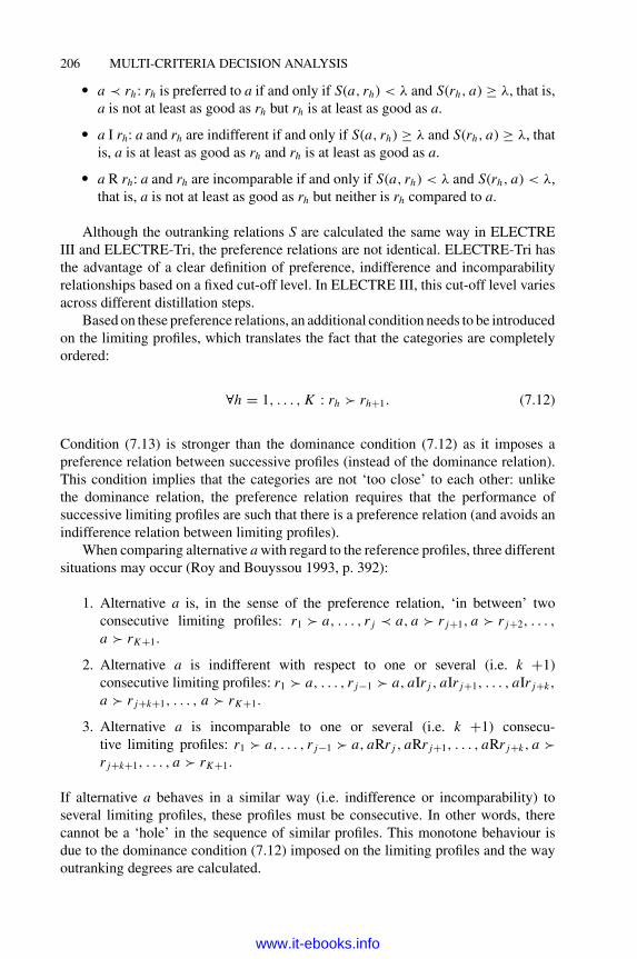
206 MULTI-CRITERIA DECISION ANALYSIS
� a ≺ rh : rh is preferred to a if and only if S(a, rh) < λ and S(rh, a) ≥ λ, that is,a is not at least as good as rh but rh is at least as good as a.
� a I rh: a and rh are indifferent if and only if S(a, rh) ≥ λ and S(rh, a) ≥ λ, thatis, a is at least as good as rh and rh is at least as good as a.
� a R rh: a and rh are incomparable if and only if S(a, rh) < λ and S(rh, a) < λ,that is, a is not at least as good as rh but neither is rh compared to a.
Although the outranking relations S are calculated the same way in ELECTREIII and ELECTRE-Tri, the preference relations are not identical. ELECTRE-Tri hasthe advantage of a clear definition of preference, indifference and incomparabilityrelationships based on a fixed cut-off level. In ELECTRE III, this cut-off level variesacross different distillation steps.Based on these preference relations, an additional condition needs to be introduced
on the limiting profiles, which translates the fact that the categories are completelyordered:
∀h = 1, . . . , K : rh � rh+1. (7.12)
Condition (7.13) is stronger than the dominance condition (7.12) as it imposes apreference relation between successive profiles (instead of the dominance relation).This condition implies that the categories are not ‘too close’ to each other: unlikethe dominance relation, the preference relation requires that the performance ofsuccessive limiting profiles are such that there is a preference relation (and avoids anindifference relation between limiting profiles).When comparing alternative awith regard to the reference profiles, three different
situations may occur (Roy and Bouyssou 1993, p. 392):
1. Alternative a is, in the sense of the preference relation, ‘in between’ twoconsecutive limiting profiles: r1 � a, . . . , r j ≺ a, a � r j+1, a � r j+2, . . . ,a � rK+1.
2. Alternative a is indifferent with respect to one or several (i.e. k +1)consecutive limiting profiles: r1 � a, . . . , r j−1 � a, aIr j , aIr j+1, . . . , aIr j+k,
a � r j+k+1, . . . , a � rK+1.
3. Alternative a is incomparable to one or several (i.e. k +1) consecu-tive limiting profiles: r1 � a, . . . , r j−1 � a, aRr j , aRr j+1, . . . , aRr j+k, a �r j+k+1, . . . , a � rK+1.
If alternative a behaves in a similar way (i.e. indifference or incomparability) toseveral limiting profiles, these profiles must be consecutive. In other words, therecannot be a ‘hole’ in the sequence of similar profiles. This monotone behaviour isdue to the dominance condition (7.12) imposed on the limiting profiles and the wayoutranking degrees are calculated.
www.it-ebooks.info

ELECTRE 207
7.5.3 Assignment rules
ELECTRE-Tri proposes two different assignment rules: the optimistic and pessimisticassignment rule. Both rules use different preference relations to compare the limitingprofiles with the alternative to be assigned. The optimistic assignment rule uses thepreference relation (�) and the pessimistic assignments rule uses the outrankingrelation (S). Both procedures handle the situation in a different way.
Optimistic assignment rule. Alternative a will be assigned to category Ch if theupper limiting profile rh is the worst (lowest) profile which is preferred to a. Formally:
� Compare successively a and rh, with h from K+1 to 1, where K+1 is the worstprofile.
� If rh is the first reference profile such that rh � a, then a is assigned to Ch.
Pessimistic assignment rule. Alternative a will be assigned to category Ch if thelower limiting profile rh+1 is the best (highest) profile, which is outranked by a orwith which a is at least as good. Formally:
� Compare successively a and rh with h from 1 to K+1.� If rh+1 is the first reference profiles such that a S rh+1, then a is assigned to Ch.
Let us consider situations 1, 2 and 3 defined in Section 7.5.2. The assignment ruleslead to the assignments given in Table 7.12. Note that the two rules lead to differentassignments in situation 3, when an alternative is incomparable to one limiting profile.In the optimistic case, it is assigned to the ‘best’ category or to the category whoselower limiting profile is the best profile to which the alternative is incomparable. Inthe pessimistic case, the alternative is assigned to the ‘worst’ category or the categorywhose upper limiting profile is the worst one to which the alternative is incomparable(i.e. rj+k).
Table 7.12 Summary of the assignment results whenusing the ELECTRE-Tri rules.
Optimistic rule Pessimistic rule
Situation 1 Cj Cj
Situation 2 Cj–1 Cj–1
Situation 3 Cj–1 Cj+k
7.5.4 Properties
ELECTRE-Tri has the following properties (Yu, 1992; Roy and Bouyssou 1993):
� Every alternative is assigned to one category according to one of the procedures(‘uniqueness property’). However, optimistic and pessimistic procedures mayassign an alternative to a different category.
www.it-ebooks.info

208 MULTI-CRITERIA DECISION ANALYSIS
� The assignment of an alternative does not depend on the assignment of theother alternatives of A. (‘independence property’).
� When two identical alternatives are compared to the reference profiles (i.e. theoutranking relations between the alternatives and the profiles are the same),they are assigned to the same categories (‘strong homogeneity property’).
� If alternative a dominates alternative b, then a will be assigned to the cate-gory which is at least as good as the category to which b will be assigned(‘monotonicity property’).
� The fusion of two successive categories or the separation of a category into twonew categories does not affect the assignment of the alternatives in the othercategories (‘stability property’).
� If the performance of alternative a is ‘between’ the performance of two con-secutive limiting profiles, it will unequivocally be assigned to the categorydelimited by these profiles (‘conformity property’).
Exercise 7.4
In this exercise, you will learn how to use the Electre-Tri software in a sortingproblem.
Learning Outcomes
� Structure a sorting problem in the Electre-Tri software (download fromhttp://www.lamsade.dauphine.fr/spip.php?rubrique64)
� Understand the steps of the sorting method ELECTRE-Tri
Tasks
a) Consider the two limiting profiles in Table 7.13, evaluated on five criteriadefining three ordered categories. In the software the best profile is denotedby rK+1 (r2 in our example) and the worst by r1. Enter the limiting profiles inthe software.
b) Consider the alternatives to be sorted, whose performance is given in the topleft matrix of Figure 7.16. Enter their performances in the software.
Table 7.13 Evaluation of the performancesof the limiting profiles.
f1 f2 f3 f4 f5
r2 15 15 15 15 15r1 10 10 10 10 10
www.it-ebooks.info
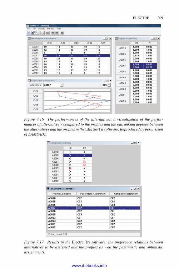
ELECTRE 209
Figure 7.16 The performances of the alternatives, a visualization of the perfor-mances of alternative 7 compared to the profiles and the outranking degrees betweenthe alternatives and the profiles in theElectre-Tri software. Reproduced by permissionof LAMSADE.
Figure 7.17 Results in the Electre Tri software: the preference relations betweenalternatives to be assigned and the profiles as well the pessimistic and optimisticassignments.
www.it-ebooks.info
210 MULTI-CRITERIA DECISION ANALYSIS
c) The parameters associated to each criterion are identical: qj = 1, pj = 2, vj
= 4, wj = 0.2. All criteria are to be maximized. The λ-threshold is set at 0.76.Enter these parameters into the software.
d) Compute the outranking degrees between the actions and limiting profiles.Check that your results are the same as in the right-handmatrix of Figure 7.16.Based on the outranking degrees, and the λ-threshold of 0.76, verify thebinary relations between the actions and limiting profiles. Check that yourresults are the same as in the upper matrix of Figure 7.17.
e) Assign the actions according to the pessimistic and optimistic assignmentrules. The results are given in the lower matrix of Figure 7.17.
References
Bouyssou, D. (1992). Ranking methods based on valued preference relations: A characteriza-tion of the net flow method. European Journal of Operational Research, 60, 61–67.
Bouyssou, D., and Perny, P. (1992). Ranking methods for valued preference relations: Acharacterization of a method based on leaving and entering flows. European Journal ofOperational Research, 61, 186–194.
Dias, J., Figueira, J., and Roy, B. (2010). Electre Tri-C: a multiple criteria sorting methodbased on central reference actions. European Journal of Operational Research, 204(3),565–580.
Figueira, J., Mousseau, V., and Roy, B. (2005). Electre methods. In J. Figueira, S. Greco, andM. Ehrgott, Multiple Criteria Decision Analysis: State of the Art Surveys (pp. 133–162).New York: Springer-Verlag.
Gabrel, V. (1990). Experimentations sur la non-independance vis-a-vis des tierces alternativeset la non-monotonicite des methodes Electre III et IV. Universite Paris-Dauphine, Memoirede DEA 103.
Giannoulis, C., and Ishizaka, A. (2010). Aweb-based decision support systemwith ELECTREIII for a personalised ranking of British universities. Decision Support Systems, 48(3), 488–497.
Hokkanen, J., and Salminen, P. (1996). ELECTRE III and IV decision aids in an environmentalproblem. Multicriteria Decision Analysis, 4, 215–226.
Kangas, A., and Pykalainen, J. (2001). Outranking methods as tools in strategic naturalresources planning. Silva Fennica, 35(2), 215–277.
Karagiannidis, A., and Moussiopoulos, N. (1997). Application of ELECTRE III for theintegrated management of municipal solid wastes in the Greater Athens area. EuropeanJournal of Operational Research, 97(11), 439–449.
Karagiannidis, A., and Papadopoulos, A. (2008). Application of the multi-criteria analysismethod ELECTRE III for the optimisation of decentralised energy systems. Omega, 5,766–776.
Mareschal, B., De Smet, Y., and Nemery, P. (2008). Rank reversal in the PROMETHEE IImethod: Some new results.Procedeeings of the IEEE International Conference on IndustrialEngineering and Engeneering Management, Singapore, 959–963, 2008.
www.it-ebooks.info

ELECTRE 211
Parent, E., and Schnabele, P. (1988). Le choix d’un amenagement aquacole: Exempled’utilisation de la methode Electre III et comparaison avec d’autres methodes multicriteresd’aide a la decision. Cahier du LAMSADE 47, Universite Paris-Dauphine.
Perny, P. (1992). Modelisation, agregation et exploitation des preferences floues dans uneproblematique de rangement: bases axiomatiques, procedures et logiciels. Universite Paris-Dauphine.
Rogers, M., and Bruen, M. (1998a). Choosing realistic values of indifference, preference andveto thresholds for use with environmental criteria within ELECTRE. European Journal ofOperational Research, 107(3), 542–551.
Rogers, M., and Bruen, M. (1998b). A new system for weighting environmental criteria foruse within Electre III. European Journal of Operational Research, 107(3), 552–563.
Roy, B. (1968). Classement et choix en presence de points de vue multiples (la methodeELECTRE). Revue d’Informatique et de Recherche Operationnelle, 2(8), 57–75.
Roy, B. (1974). Criteres multiples et modelisation des preferences: l’apport des relations desurclassment. Revue d’Economie Politique, 1, 1–44.
Roy, B., and Bouyssou, D. (1993). Aide multicritere a la decision: Methodes et cas. Paris:Economica.
Tervoren, T., Figueira, J., Lahdelma, R., and Salminem, R. (2004). An inverse approach forELECTRE III. Technical report.
Wand, X., and Triantaphyllou, E. (2006). Ranking irregularities when evaluating alternativesby using some Electre methods. International Journal of Management Science, 36, 45–63.
Yu, W. (1992). Aide multicritere a la decision dans le cadere de la problematique du tri:concepts, methodes et applications. PhD thesis, UER Sciences de l’organisation, Universitede Paris Dauphine.
www.it-ebooks.info

Part III
GOAL, ASPIRATION ORREFERENCE-LEVELAPPROACH
Multi-Criteria Decision Analysis: Methods and Software, First Edition. Alessio Ishizaka and Philippe Nemery.© 2013 John Wiley & Sons, Ltd. Published 2013 by John Wiley & Sons, Ltd.
www.it-ebooks.info

8
TOPSIS
8.1 Introduction
This chapter explains the theory and practical uses of TOPSIS, which stands for‘Technique of Order Preference Similarity to the Ideal Solution’. In this chapterMicrosoft Excel is used to illustrate problem solving with TOPSIS, while DECERNS,one of the few available software packages supporting TOPSIS, is described inChapter 11. TOPSIS is not based on a complex algorithm and therefore a ‘black box’section is unnecessary.
The companion website provides an illustrative example with Microsoft Excel.
8.2 Essentials of TOPSIS
The TOPSIS method requires only a minimal number of inputs from the user andits output is easy to understand. The only subjective parameters are the weightsassociated with the criteria. Several applications can be found in Behzadian et al.(2012). The fundamental idea of TOPSIS is that the best solution is the one whichhas the shortest distance to the ideal solution and the furthest distance from the anti-ideal solution (Hwang and Yoon 1981; Lai et al. 1994; Yoon 1980). For example,in Figure 8.1, where both criteria are to be maximized, alternative A is closer to theideal solution than B and further from the anti-ideal solution if the criteria weightsare equivalent. As a result, TOPSIS presents alternative A as a better solution thanalternative B.
The TOPSIS method is illustrated by Case Study 8.1.
Multi-Criteria Decision Analysis: Methods and Software, First Edition. Alessio Ishizaka and Philippe Nemery.© 2013 John Wiley & Sons, Ltd. Published 2013 by John Wiley & Sons, Ltd.
www.it-ebooks.info

216 MULTI-CRITERIA DECISION ANALYSIS
Ideal solution
Anti-ideal solution
A
B
criterion 2
criterion 1
1
1
Figure 8.1 TOPSIS method.
Case Study 8.1
A company wants to recruit a new principal assistant for its international market.Four candidates have been shortlisted: Anna, Tom, Jack and Emma. Four criteriahave been selected to make the decision. As the post requires intensive contactwith various customers, it is necessary for the principal assistant to have stronginterpersonal skills, with the ability to interact effectively with diverse clientstyles within different working environments. The role involves dealing with theinternational market, and as a result, extensive experience of living abroad wouldbe advantageous. Similar work experience would be beneficial. Each candidate isrequired to sit a written exam to assess their knowledge of international culture.The performances of each candidate against the four criteria are shown in Table 8.1.
Table 8.1 Weights of the criteria and performances of the alternatives.
Interpersonal skills Living abroad Written test Work experience(score out of 10) (years) (score out of 10) (years)
Weight 0.1 0.4 0.3 0.2
Anna 7 9 9 8Tom 8 7 8 7Jack 9 6 7 12Emma 6 11 8 6
www.it-ebooks.info
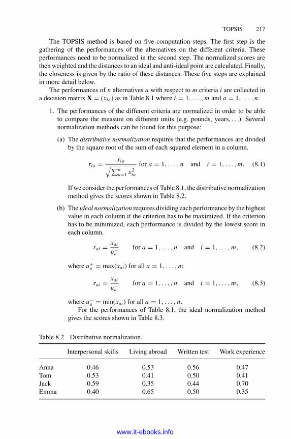
TOPSIS 217
The TOPSIS method is based on five computation steps. The first step is thegathering of the performances of the alternatives on the different criteria. Theseperformances need to be normalized in the second step. The normalized scores arethen weighted and the distances to an ideal and anti-ideal point are calculated. Finally,the closeness is given by the ratio of these distances. These five steps are explainedin more detail below.
The performances of n alternatives a with respect to m criteria i are collected ina decision matrix X = (xia) as in Table 8.1 where i = 1, . . . , m and a = 1, . . . , n.
1. The performances of the different criteria are normalized in order to be ableto compare the measure on different units (e.g. pounds, years, . . .). Severalnormalization methods can be found for this purpose:
(a) The distributive normalization requires that the performances are dividedby the square root of the sum of each squared element in a column.
ria = xia√∑na=1 x2
ia
for a = 1, . . . , n and i = 1, . . . , m. (8.1)
If we consider the performances of Table 8.1, the distributive normalizationmethod gives the scores shown in Table 8.2.
(b) The ideal normalization requires dividing each performance by the highestvalue in each column if the criterion has to be maximized. If the criterionhas to be minimized, each performance is divided by the lowest score ineach column.
rai = xai
u+a
for a = 1, . . . , n and i = 1, . . . , m, (8.2)
where u+a = max(xai ) for all a = 1, . . . , n;
rai = xai
u−a
for a = 1, . . . , n and i = 1, . . . , m, (8.3)
where u−a = min(xai ) for all a = 1, . . . , n.
For the performances of Table 8.1, the ideal normalization methodgives the scores shown in Table 8.3.
Table 8.2 Distributive normalization.
Interpersonal skills Living abroad Written test Work experience
Anna 0.46 0.53 0.56 0.47Tom 0.53 0.41 0.50 0.41Jack 0.59 0.35 0.44 0.70Emma 0.40 0.65 0.50 0.35
www.it-ebooks.info

218 MULTI-CRITERIA DECISION ANALYSIS
Table 8.3 Ideal normalization.
Interpersonal skills Living abroad Written test Work experience
Anna 0.78 0.82 1.00 0.67Tom 0.89 0.64 0.89 0.58Jack 1.00 0.55 0.78 1.00Emma 0.67 1.00 0.89 0.50
2. Now the weights are taken into account: A weighted normalized decisionmatrix is constructed by multiplying the normalized scores rai by their corre-sponding weights wi :
vai = wi · rai . (8.4)
For the distributive normalized scores, we obtain the weighted scores shownin Table 8.4.
3. The weighted scores will be used to compare each action to an ideal (zenith) andanti-ideal (or nadir or negative ideal) virtual action. There are three differentways of defining these virtual actions.
(a) By collecting the best and worst performance on each criterion of thenormalized decision matrix. For the ideal action we have
A+ = (v+
1 , . . . , v+m
), (8.5)
and for the anti-ideal action
A− = (v−
1 , . . . , v−m
), (8.6)
where v+i = maxa(vai ) if criterion i is to be maximized and v−
i = mina(vai )if criterion i is to be minimized.
(b) Assuming an absolute ideal and anti-ideal point, which are defined withoutconsidering the actions of the decision problem, A+ = (1, . . . , 1) andA− = (0, . . . , 0)
(c) The ideal and anti-ideal points are defined by the decision maker. Thesepoints must be between the ideal and anti-ideal points calculated with thetwo other methods explained above. This method is not often used as itrequires an input from the user, which is often difficult to elicit.
4. Calculate the distance for each action to the ideal action,
d+a =
√∑i
(v∗i − vai )2, a = 1, . . . , m, (8.7)
www.it-ebooks.info

TOPSIS 219
Table 8.4 Weighted normalized scores.
Interpersonal skills Living abroad Written test Work experience
Anna 0.046 0.213 0.168 0.093Tom 0.053 0.165 0.149 0.082Jack 0.059 0.142 0.131 0.140Emma 0.040 0.260 0.149 0.070
and the anti-ideal action,
d−a =
√∑i
(v−i − vai )2, a = 1, . . . , m. (8.8)
In (8.7) and (8.8), we use a Euclidean distance (L2), which is the most popular,but another metric could be adopted (e.g. L1, the Manhattan metric).
5. Calculate the relative closeness coefficient of each action:
Ca = d−a
d+a + d−
a. (8.9)
The closeness coefficient is always between 0 and 1, where 1 is the pre-ferred action. If an action is closer to the ideal than the anti-ideal, then Ca
approaches 1, whereas if an action is closer to the anti-ideal than to the ideal, Ca
approaches 0.
Table 8.5 contains the ideal and anti-ideal action with the ideal and distributivenormalization. Table 8.6 contains the details of the closeness calculation. Emma isthe selected action independently of the normalization adopted.
TOPSIS has been criticized because it sometimes gives illogical results. Opri-covic and Tzeng (2004) presented a simple example where an extreme action (A1),evaluated on two similarly weighted criteria, is preferred over a superior compro-mise (A2). In a slightly modified example (Table 8.7), Figure 8.2, produced withDECERNS, shows that compromise A2 will never be ranked first indifferently of theassigned weights.
Table 8.5 Ideal and anti-ideal action.
Ideal normalization Distributive normalization
Interpersonal Living Written Work Interpersonal Living Written Workskills abroad test experience skills abroad test experience
A+ 0.100 0.400 0.300 0.200 0.059 0.260 0.168 0.140A− 0.067 0.218 0.233 0.100 0.040 0.142 0.131 0.070
www.it-ebooks.info

220 MULTI-CRITERIA DECISION ANALYSIS
Table 8.6 Closeness calculation.
Ideal normalization Distributive normalization
Anna Tom Jack Emma Anna Tom Jack Emma
d+a 0.101 0.171 0.194 0.111 0.068 0.113 0.124 0.075
d−a 0.133 0.057 0.105 0.185 0.084 0.035 0.073 0.120
Ca 0.507 0.250 0.350 0.630 0.550 0.240 0.370 0.610
Table 8.7 Table of scores.
A1 A2 A3
Criterion 1 (to be maximized) 3000 3750 4500Criterion 2 (to be minimized) 1 2 5
Figure 8.2 TOPSIS prefers never prefers the comprmise A2. Reproduced by permis-sion of Boris Yatsalo.
www.it-ebooks.info

TOPSIS 221
Finally, we remark that using the Euclidean distance, as in (8.7) and (8.8), whichmagnifies large distances (Lai et al. 1994), may lead to different results than methodsbased on Manhattan distances (L1).
Exercise 8.1
First you will familiarize yourself with the step-by-step TOPSIS calculations inMicrosoft Excel and then have an opportunity to complete the spreadsheet for theother criteria.
Learning Outcomes
� Understand the calculation of the closeness with a distributive normalization
� Understand the calculation of the closeness with an ideal normalization
� Understand the calculation of the closeness with an ideal and absolute idealsolution
Tasks
Open the file Recruitment.xls. It contains four spreadsheets with variants ofTOPSIS.
Answer the following questions:
a) Describe the meaning of each calculation cell and its formula. Compare thefour variants.
b) Customize the spreadsheets for a problem of your choice.
References
Behzadian, M., Otaghsara, K., Yazdani, M., and Ignatius, J. (2012). A state-of the-art surveyof TOPSIS applications. Expert Systems with Applications, 39(17), 13051–13069.
Hwang, C.-L., and Yoon, K. (1981). Multiple Attribute Decision Making: Methods andApplications. New York: Springer-Verlag.
Lai, Y.-J., Liu, T.-Y., and Hwang, C.-L. (1994). TOPSIS for MODM. European Journal ofOperational Research, 76(3), 486–500.
Opricovic, S., and Tzeng, G.-H. (2004). Compromise solution by MCDM methods: A compar-ative analysis of VIKOR and TOPSIS. European Journal of Operational Research, 156(2),445–455.
Yoon, K. (1980). Systems selection by multiple attribute decision making. Kansas StateUniversity.
www.it-ebooks.info

9
Goal programming
9.1 Introduction
This chapter explains the theory and practical use of the goal programming meth-ods. After a theoretical section, Section 9.3 explains how to solve goal programmingproblems with Microsoft Excel. Three variants of goal programming are presented.This chapter does not include a black box section as the algorithm behind the goalprogramming is the well-known simplex method (see Ignizio and Cavalier 1994;Schniederjans 1984). Since goal programming is an extension of linear program-ming to handle multiple conflicting objectives, the reader is advised to first read theAppendix on linear programming to ensure a better understanding.The companion website provides illustrative examples with Microsoft Excel.
9.2 Essential concepts of goal programming
The idea of goal programming is that there is an ideal goal to be achieved while alsosatisfying hard constraints. This goal is composed of several objectives that may beconflicting. The main difficulty is the modelling of the problem: to find the goal andthe soft and hard constraints. Case Study 9.1 will be used to illustrate this point.
Case Study 9.1
A company produces two types of product: A and B. To manufacture, product Arequires 5 parts of type I and 3 parts of type II; B requires 4 parts of type I and 2parts of type II. The profit is £20 for A and £30 for B. The company aims to achievea weekly profit of £2000. The production time per unit of A is 7 man-hours and perunit of B is 3 man-hours. The company employs seven people in the productiondepartment and would like to keep within the 250 available hours of work each
Multi-Criteria Decision Analysis: Methods and Software, First Edition. Alessio Ishizaka and Philippe Nemery.© 2013 John Wiley & Sons, Ltd. Published 2013 by John Wiley & Sons, Ltd.
www.it-ebooks.info

GOAL PROGRAMMING 223
week. A contract has been signed with a supplier to deliver up to 80 parts of typeI and 60 parts of type II. It is possible to order more parts but they would be muchmore expensive. The manufacturing capacity of the machine for both productscombined is limited to a maximum of 80 products per week. The company has astrategic target to produce at least 50 units of each product per week.
The modelling of the problem requires first the identification of the decisionvariables, goals and constraints.
Identification of the decision variables. The decision variables are indepen-dent variables that are changed until the desired quantity is obtained. InCase Study 9.1, they are given by x1, the number of units of product A manu-factured per week, and x2, the number of units of product B manufactured perweek.
Identification of the goals and soft and hard constraints. A hard constraint is aninequality that describes a threshold that cannot be exceeded as it represents anunfeasible region of solution. All solutions below the threshold have the samepreference. A goalwith a soft constraint has a threshold which is an ideal point,but can be exceeded because solutions over this point are feasible even if theyare not attractive. In this case, both deviational variables should be added. Whyshould unattractive solutions be accepted? As there are often several goals, notall can be achieved simultaneously; therefore, some good solutions may beunattractive to some goals. A goalwith a hard constraint has a threshold whichis an ideal point and cannot be exceeded. The nearest solutions to the idealpoint are preferred. In this case, only the deviational variable to be minimizedshould be introduced into the equation.
In Case Study 9.1, there are seven constraints:
� The profit target of the company of £2000 sets the first constraint:
30x1 + 20x2 ≥ 2000.
Is this a soft or hard constraint? The company will still survive if the benefit islower; therefore it is a desirable goal. The inequality can be transformed intoan equality with two adjustment variables: n1 for a negative deviation of thegoal and p1 for a positive deviation:
30x1 + 20x2 + n1 − p1 = 2000.
One direction of the deviation will be preferred over the other. In this case, itis preferable to have a greater than a lesser benefit. The deviational variable n1is thus to be minimized.
www.it-ebooks.info

224 MULTI-CRITERIA DECISION ANALYSIS
� The second constraint is set by the total working hours in a week:
7x1 + 3x2 ≤ 250.
Again, is it a soft or hard constraint? As employees can do overtime or tempo-rary staff can be hired, this inequality can be considered a goal and transformedinto:
7x1 + 3x2 + n2 − p2 = 250.
In this case, the extra hours variable (p2) is the deviational variable tominimize.
� The next two constraints are set by the capacity of the suppliers: for parts oftype I,
5x1 + 4x2 ≤ 80;
For parts of type II,
3x1 + 2x2 ≤ 60.
As the suppliers are able to deliver additional parts, these are soft constraintsand can be transformed into:
5x1 + 4x2 + n3 − p3 = 80,
3x1 + 2x2 + n4 − p4 = 60.
Additional parts are more expensive and as a result, the positives deviations p3and p4 are to be minimized.
� The following two constraints are set by the strategic aims of the company,which is to produce a minimum of 50 units of product A and B. The constraintscan be written as:
x1 ≥ 50,x2 ≥ 50.
It is possible to produce less, therefore the constraints above are transformedinto goals:
x1 + n5 − p5 = 50,
x2 + n6 − p6 = 50.
www.it-ebooks.info

GOAL PROGRAMMING 225
� The last constraint is set by the capacity of the machine:
x1 + x2 ≤ 80.
This is a hard constraint because the machine cannot produce more than itscapacity. Therefore, it cannot be transformed into a goal.
Putting all goals and constraints together, we have the following goal program:
min z = n1 + p2 + p3 + p4 + n5 + n6
subject to:
30x1 + 20x2 + n1 − p1 = 2000
7x1 + 3x2 + n2 − p2 = 250
5x1 + 4x2 + n3 − p3 = 80
3x1 + 2x2 + n4 − p4 = 60
x1 + n5 − p5 = 50
x2 + n6 − p6 = 50
x1 + x2 ≤ 80x1, x2 ≤ 0ni , pi ≥ 0, i = 1, . . . , 6.
Note that the goal program does not contain any weight. They will be introduced inthe section 9.4.1. In the program modelling, supplementary constraints are added toensure that all decisional and deviational variables are positives.It is important to transform hard constraints into goals where possible. This allows
the examination of a larger solution space, which may contain potentially good oroptimal solutions. It is also important to incorporate both deviational variables n andp, when possible, for the same reason.The goal programming method cannot detect a Pareto front. A Pareto front
contains the set of solutions that, when compared to other solutions, are at leastas good with respect to all objectives and strictly better with respect to at leastone objective. This is problematic if the goals are set too low because a bettersolution may exist but will not be proposed as it is too far from the goal set bydecision maker. For example, if the Pareto optimum is at profit of £10 000, itwill not be detected if the decision maker sets a low goal as £2000. Techniqueshave been developed to detect and restore the Pareto inefficiency (Hannan 1980;Romero 1991).
www.it-ebooks.info

226 MULTI-CRITERIA DECISION ANALYSIS
Exercise 9.1
The following multiple-choice questions allow you to test your knowledge on thebasics of goal programming. Only one answer is correct. Answers can be found onthe companion website.
1. How many deviational variables are in the objective function of goal program-ming?
a) Equivalent to the number of goals
b) Twice the number of goals
c) Equivalent to the number of soft and hard constraints
d) Twice the number of soft and hard constraints
2. What is a soft constraint?
a) An inequality
b) A constraint with a threshold indicating unfeasible solutions
c) A goal
d) A constraint that is not needed in the modelling of the problem
3. Which statement is incorrect?
a) All deviational variables should be included in the equation
b) A hard constraint is not a goal
c) Several solutions may exist
d) All goals are always satisfied
4. What type of problems can goal programming solve?
a) Problems with a discrete solution space
b) Problems with continuous solution space
c) Problems with a binary solution space
d) Sorting problems
5. Goal programming is a generalization of which method?
a) MACBETH
b) Linear programming
c) TOPSIS
d) DEA
www.it-ebooks.info

GOAL PROGRAMMING 227
Figure 9.1 Microsoft Excel spreadsheet for the Case Study 9.1 goal program.
9.3 Software description
Linear goal programs can be solved using linear programming software, for exam-ple the Microsoft Excel Solver add-in or LINGO package. The widespread use andknowledge ofMicrosoft Excel is themain reason to opt for theMicrosoft Excel Solver.This section describes how to use it.
9.3.1 Microsoft Excel Solver
To explain theMicrosoft Excel Solver, Case Study 9.1 will be used. The essential firststep to solving a goal programming problem is correct modelling. A goal programmust be written by hand as in Section 9.2 as the software is unable to do this. Whenit has been defined, it must be rewritten in aMicrosoft Excel spreadsheet. There is nostrict rule on how to enter it, but it is helpful to have a clear structure.In Figure 9.1:
� Line 4 determines the deviational variables to be minimized. In this case, theyall have the same weight. Section 9.4 describes how to weight them differently.
� Lines 5–10 contain the goals, and line 11 the hard constraint.
� Line 13 contains the decision and deviational variables that need to be foundby the solver.
� Cell E15 represents the objective to minimized, which is the sum of n1, n5, n6,p2, p3 and p4. This information is entered in the Solver parameters shown inFigure 9.2.
Exercise 9.2
You will learn the use of theMicrosoft Excel Solver for solving goal programs.
Learning Outcomes
� Understand the modelling of a goal programme
� Understand the parameters in Microsoft Excel Solver
www.it-ebooks.info

228 MULTI-CRITERIA DECISION ANALYSIS
Figure 9.2 Solver parameters.
Tasks
Open the file Production.xls on the un-weighted GP tab. It contains a spreadsheetwith the goal programme of the problem of the Case Study 9.1.Answer the following questions:
a) In the spreadsheet, find the objective of the problem, the decision variables,the goals and hard constraints. (Read the comments in the red square in caseof difficulty.)
b) Open the Solver. What is entered in the set target cell? What is entered in thebox ‘by changing cells’? What is entered in the box ‘Subject to constraints?’
9.4 Extensions of the goal programming
As not all goals have the same importance, several variants have been conceived toweight goals differently (Jones and Mehrdad 2010).
9.4.1 Weighted goal programming
In weighted goal programming, penalty weights are attached to the unwanted devi-ational variables. These weights are composed of two parts: a conversion factor inorder to assure a commensurability of the deviational variables, and the importanceof the penalization given at each deviation.There are different ways to normalize deviational variables. A practical way is
to use percentage normalization, which indicates the percentage away from the goal.For this purpose, the deviational variable is divided by the goal of the objective. The
www.it-ebooks.info

GOAL PROGRAMMING 229
weights are set in the numerator part. For example, in Case Study 9.1, we consider1% deviation from the target of 250h/week is five times more important than theother goals. The new weighted goal program is:
min z = 1
2000n1 + 5
250p2 + 1
80p3 + 1
60p4 + 1
50n5 + 1
50n6
subject to:
30x1 + 20x2 + n1 − p1 = 2000
7x1 + 3x2 + n2 − p2 = 250
5x1 + 4x2 + n3 − p3 = 80
3x1 + 2x2 + n4 − p4 = 60
x1 + n5 − p5 = 50
x2 + n6 − p6 = 50
x1 + x2 ≤ 80x1, x2 ≥ 0ni , pi ≥ 0, i = 1, . . . , 6
(the deviational variables to be minimized are in bold).
Exercise 9.3
You will learn the use of the Microsoft Excel Solver for solving a weighted goalprogram.
Learning Outcomes
� Understand the modelling of a weighted goal program
� Understand the parameters in Microsoft Excel Solver
Tasks
Open the file Production.xls on the weighted GP tab. It contains a spreadsheetwith the weighted goal program of the problem in Case Study 9.1.Answer the following questions:
a) In the spreadsheet, find the objective of the problem, the decision variables,the goals, the hard constraints and weights. (Read the comments in the redsquare in case of difficulty.)
b) How has the optimal result changed?
www.it-ebooks.info

230 MULTI-CRITERIA DECISION ANALYSIS
9.4.2 Lexicographic goal programming
The lexicographic goal programming is used when the decision maker has a clearpreference order for satisfying the goals. For example, in Case Study 9.1, the goal ofthe total working hours in a week is strictly preferable to the other goals because thestaff could strike. The first step is to minimize this goal:
min z = p2
Subject to:
30x1 + 20x2 + n1 − p1 = 2000
7x1 + 3x2 + n2 − p2 = 250
5x1 + 4x2 + n3 − p3 = 80
3x1 + 2x2 + n4 − p4 = 60
x1 + n5 − p5 = 50
x2 + n6 − p6 = 50
x1 + x2 ≤ 80x1, x2 ≥ 0ni , pi ≥ 0, i = 1, . . . , 6
(the deviational variables to be minimized are in bold).An optimum is found at p2 = 0. Then the second priority level is optimized. This
goal program has all the goals and constraints of the previous formulation plus theadditional constraint p2 = 0:
min z = n1 + p3 + p4 + n5 + n6
subject to:
30x1 + 20x2 + n1 − p1 = 2000
7x1 + 3x2 + n2 − p2 = 250
5x1 + 4x2 + n3 − p3 = 80
3x1 + 2x2 + n4 − p4 = 60
x1 + n5 − p5 = 50
x2 + n6 − p6 = 50
x1 + x2 ≤ 80p2 = 0
x1, x2 ≥ 0ni , pi ≥ 0, i = 1, . . . , 6.
www.it-ebooks.info

GOAL PROGRAMMING 231
Figure 9.3 Lexographic goal program, first-level priority.
Figure 9.4 Lexographic goal program, second-level priority.
InMicrosoft Excel, each priority level is solved in a new spreadsheet (Figure 9.3and Figure 9.4). The model is solved for each priority level at a time by adding aconstraint in the spreadsheet (line 18 in Figure 9.4) and in theMicrosoft Excel Solverparameters box. For a large number of priority levels, the process can be automatedby programming a macro in Visual Basics for Applications.
Exercise 9.4
You will learn the use of theMicrosoft Excel Solver for solving a lexicographic goalprogram.
Learning Outcomes
� Understand the modelling of a lexicographic goal program
� Understand the parameters in Microsoft Excel Solver
www.it-ebooks.info

232 MULTI-CRITERIA DECISION ANALYSIS
Tasks
Open the file Production.xls on the LGP1 and LGP12 tabs. It contains two spread-sheets with the lexicographic goal program of the problem in Case Study 9.1.Answer the following questions:
a) In the two spreadsheets, find the objective of the problem, the decision vari-ables, the goals, the hard constraints and weights. (Read the comments in thered square in case of difficulty.)
b) Compare the Solver box of the two spreadsheets. How do the parametersdiffer?
c) How has the optimal result changed from the traditional goal program?
9.4.3 Chebyshev goal programming
Unweighted, weighted and lexographic goal programming often find extreme points(intersections of goals, constraints and axes), which lead to an unbalanced solution:some goals are achieved and others are far from satisfactory. In order to counter thisproblem, Chebyshev goal programming has been developed (Flavell 1976). The ideaof this method is to introduce additional constraints to the model to ensure a balancebetween the objectives.If we assume equal preferential weights and a percentage normalization, the
Chebyshev goal programme of Case Study 9.1 is given by:
min z = λ
subject to:
1
2000n1 ≤ λ
5
250p2 ≤ λ
1
80p3 ≤ λ
1
60p4 ≤ λ
1
50n5 ≤ λ
1
50n6 ≤ λ
30x1 + 20x2 + n1 − p1 = 2000
7x1 + 3x2 + n2 − p2 = 250
5x1 + 4x2 + n3 − p3 = 80
www.it-ebooks.info

GOAL PROGRAMMING 233
Figure 9.5 Chebyshev goal program.
3x1 + 2x2 + n4 − p4 = 60
x1 + n5 − p5 = 50
x2 + n6 − p6 = 50
x1 + x2 ≤ 80p2 = 0
x1, x2 ≥ 0ni , pi ≥ 0, i = 1, . . . , 6
(the deviational variables to be minimized are in bold). In theMicrosoft Excel spread-sheet, the additional constraints are also added (lines 13–18 in Figure 9.5).
Exercise 9.5
You will learn the use of the Microsoft Excel Solver for solving a Chebyshev goalprogram.
Learning Outcomes
� Understand the modelling of a Chebyshev goal program
� Understand the parameters in Microsoft Excel Solver
Tasks
Open the file Production.xls on the Chebyshev tab. It contains a spreadsheet withthe Chebyshev goal program of the problem in Case Study 9.1.
www.it-ebooks.info
234 MULTI-CRITERIA DECISION ANALYSIS
Answer the following questions:
a) In the spreadsheet, find the objective of the problem, the decision variables,the goals, the hard constraints and weights. (Read the comments in the redsquare in case of difficulty.)
b) Open the Solver in the spreadsheets. How have the parameters of the Solverboxes been changed compared to Exercise 9.2?
c) How has the optimal result changed from the traditional goal program?
References
Flavell, R. (1976). A new goal programming formulation. Omega, 4(6), 731–732.
Hannan, E. (1980). Non-dominance in goal programming. INFOR, 18(4), 300–309.
Ignizio, J., and Cavalier, T. (1994). Linear programming. Englewood Cliffs, NJ: Prentice Hall.
Jones, D., and Mehrdad, T. (2010). Practical Goal Programming. New York: Springer-Verlag.
Romero, C. (1991). Handbook of Critical Issues in Goal Programming. Oxford: PergamonPress.
Schniederjans, M. (1984). Linear Goal Programming. Princeton, NJ: Petrocelli Books.
www.it-ebooks.info

10
Data Envelopment AnalysisJean-Marc Huguenin1
10.1 Introduction
This chapter introduces a performance measurement technique called DEA, whichstands for ‘Data Envelopment Analysis’. Firm efficiency is defined as the ratio of thesum of its weighted outputs to the sum of its weighted inputs (Thanassoulis et al.2008, p. 264). As Giannoulis and Ishizaka (2010) point out, the analogy with othermulti-criteria methods is striking: firms can be considered as alternatives, outputs ascriteria to be maximized and inputs as criteria to be minimized. What distinguishesDEA is that the weights assigned to outputs and inputs are not allocated by users.Moreover, it does not rely on a common set of weights for all firms. Instead, a differentset of weights is calculated by a linear optimization procedure in order to show eachfirm in its best possible light.DEA helps decision makers in the following ways:
� By calculating an efficiency score, it indicates if a firm is completely efficientor has capacity for improvement.
1Jean-Marc Huguenin is a Senior Lecturer and a Project Manager at the Swiss Graduate Schoolof Public Administration at the University of Lausanne, Switzerland. He also heads the IndependentEconomists, an economic intelligence unit founded in 1999. He was previously an economist at the SwissNational Bank, an economist for the Swiss in-service training centre for secondary school teachers andan economics professor at the College of Bienne, Switzerland. His areas of research and expertise are theevaluation of productivity and efficiency of organizations and the economics andmanagement of educationsystems.
Multi-Criteria Decision Analysis: Methods and Software, First Edition. Alessio Ishizaka and Philippe Nemery.© 2013 John Wiley & Sons, Ltd. Published 2013 by John Wiley & Sons, Ltd.
www.it-ebooks.info

236 MULTI-CRITERIA DECISION ANALYSIS
� By setting target values for input and output, it calculates by how much inputmust be decreased or output increased in order to become efficient.
� By identifying the nature of returns to scale, it indicates if a firm has to decreaseor increase its scale (or size) in order to minimize the average total cost.
� By identifying a set of benchmarks, it specifies which other firms’ processesneed to be analyzed in order to improve its own practices.
After this introduction, Section 10.2 presents the essentials of DEA, alongside acase study to give an intuitive understanding of its application. Section 10.3 introducesWin4DEAP, a software package that conducts efficiency analysis based on DEAmethodology. Section 10.4 is designed for more demanding readers interested in themethodological background ofDEA. Finally, four advancedDEA topics are presentedin Section 10.5: adjustment to the environment, preferences, sensitivity analysis andtime series data.The companion website provides a case study using Win4DEAP, solutions to
exercises, and an illustrative example using Microsoft Excel Solver.
10.2 Essential concepts of DEA
10.2.1 An efficiency measurement method
DEA is used to measure the performance of firms or entities (called decision-makingunits, DMUs) which convert multiple inputs into multiple outputs. It is suitable forthe use of both private sector firms and public sector organizations (and even forentities such as regions or countries). DEA was formulated in Charnes et al. (1978,1981) in order to evaluate a US federal government programme in the educationsystem called ‘Program Follow Through’. The use of DEA then spread to otherpublic organizations (hospitals, elderly care facilities, social service units, unem-ployment offices, police forces, army units, prisons, waste management services,power plants, public transportation companies, forestry companies, libraries, muse-ums, theatres, etc.) and to the private sector (banks, insurance companies, retailstores, etc.).EachDMU’s efficiency score is calculated relative to an efficiency frontier. DMUs
located on the efficiency frontier have an efficiency score of 1 (or 100%). DMUsoperating beneath the frontier have an efficiency score less than 1 and so have thecapacity to improve future performance. Note that no DMU can be located above theefficiency frontier because they cannot have an efficiency score greater than 1. DMUslocated on the frontier serve as benchmarks – or peers – for inefficient DMUs. Thesebenchmarks (i.e. real DMUs with real data) are associated with best practices. DEAis therefore a powerful benchmarking technique.
www.it-ebooks.info

DATA ENVELOPMENT ANALYSIS 237
10.2.2 A DEA case study
To better understand the mechanics behind DEA, this section presents a simplepractical case study. It includes only one input and one output, although DEA canhandle multiple inputs and multiple outputs.
Case Study 10.1
FiveRegisterOffices (A toE) produce one output (total number of documents, suchas marriage or birth certificates) with one input (number of full-time equivalentpublic servants).2 The data are listed in Table 10.1. For example, first row of thetable shows that two public servants work in Register Office A. They produce onedocument (during a certain period of time).
Table 10.1 Five Register Offices produce documents with public servants.
Input Output
Register Office Public servants (x) Documents (y)
A 2 1B 3 4C 5 5D 4 3E 6 7
10.2.2.1 Two basic DEA models
Two basic models are used in DEA, leading to the identification of two differentfrontiers:
� The first model assumes constant returns to scale (CRS model). This is appro-priate when all DMUs are operating at an optimal scale. However, note thatthis is quite an ambitious assumption. To operate at an optimal scale, DMUsshould evolve in a perfectly competitive environment, which is seldom thecase. The CRS model calculates an efficiency score called constant returns toscale technical efficiency (CRSTE).
� The second model assumes variable returns to scale (VRS model). This isappropriate when DMUs are not operating at an optimal scale. This is usually
2 In order to represent this example in a two-dimensional graph, we consider a total of two outputs andinputs (one output, one input; no variable representing the quality of the variables).
www.it-ebooks.info

238 MULTI-CRITERIA DECISION ANALYSIS
the case when DMUs face imperfect competition, government regulations, etc.The VRS model calculates an efficiency score called variable returns to scaletechnical efficiency (VRSTE).
Comparison between the two models reveals the source of inefficiency. CRSTEcorresponds to the global measure of a DMU performance. It is composed of a ‘pure’technical efficiency measure (captured by the VRSTE score) and a scale efficiency(SE) measure. Section 10.2.2.6) demonstrates how these three notions (CRSTE,VRSTE and SE) relate to each other.
10.2.2.2 Input or output orientation
A DEA model can be input- or output-oriented:
� In an input orientation, DEA minimizes input for a given level of output; inother words, it indicates how much a DMU can decrease its input for a givenlevel of output.
� In an output orientation, DEA maximizes output for a given level of input; inother words, it indicates how much a DMU can increase its output for a givenlevel of input.
The efficiency frontier will be different in a CRS or a VRS model (see Section10.2.2.6). However, within each model, the frontier will not be affected by an inputor an output orientation. DMUs located on the frontier in an input orientation willalso be on the frontier in an output orientation.In a CRS model, technical efficiency scores have the same values in an input
or an output orientation. But these values will be different according to the model’sorientation when VRS is assumed. However, Coelli and Perelman (1996, 1999) notethat, in many instances, the choice of orientation has only a minor influence upon thetechnical efficiency scores calculated.The model’s orientation should be chosen according to which variables (inputs
or outputs) the decision maker has most control over. For example, a school prin-cipal will probably have more control over his teaching staff (input) than over thenumber of pupils (output). An input orientation will be more appropriate in thiscase.In the public sector, but sometimes also in the private sector, a given level of input
can be assigned and secured to a DMU. In this case, the decision maker may wantto maximize the output (and therefore choose an output orientation). Alternatively, ifthe decision maker’s task is to produce a given level of output (e.g. a quota) with theminimum input, he will opt for an input orientation.If the decision maker is not facing any constraints and has control of both input
and output, the model’s orientation will depend on his objectives. Does he needto cut costs (input orientation) or does he want to maximize production (outputorientation)?
www.it-ebooks.info

DATA ENVELOPMENT ANALYSIS 239
10.2.2.3 CRS efficient frontier
Figure 10.1 shows the efficient frontier for Case Study 10.1 assuming constant returnsto scale (CRS efficient frontier). The CRS efficient frontier starts at the origin andruns through Register Office B. Register Office B happens to be the observationwith the steepest slope, or the highest productivity ratio, among all Register Office(4/3 = 1.33, meaning that one public servant produces 1.33 document). RegisterOffice B is on the frontier; it is 100% efficient. Register Offices A, C, D and Eare below the frontier. Their respective efficiency scores are less than 100%. DEAassumes that the production possibility set is bounded by this frontier. This actuallyimplies that DEA calculates relative and not absolute efficiency scores. AlthoughDMUs on the efficient frontier are assigned a 100% efficiency score, it is likely thatthey could further improve their productivity.Figure 10.1 also illustrates how DEA measures efficiency scores. The example
of Register Office A is described below:
� In an input orientation, A’s efficiency score is equal to the distance SACRS-Idivided by the distance SA. ACRS-I is the projection of point A on the efficientfrontier (assuming constant returns to scale and an input orientation). Notethat one can easily calculate efficiency scores using a ruler and measuring thedistances on the graph. A’s score is 37.5%. This means that Register OfficeA could reduce the number of public servants employed (input) by 62.5%(100 – 37.5) and still produce the same number of documents (1).
� In an output orientation, A’s efficiency score is equal to the distance TA dividedby the distance TACRS-O. ACRS-O is the projection of point A on the efficient
0
1
2
3
4
5
6
7
8
543210Public servants
Doc
umen
ts
A
B
C
D
E
CRS efficient frontier
ACRS-IS
ACRS-O
T
76
Figure 10.1 Register Offices beneath the efficient frontier have the capacity toimprove performance.
www.it-ebooks.info

240 MULTI-CRITERIA DECISION ANALYSIS
frontier (assuming constant returns to scale –CRS– and an output orientation).A’s score is 37.5%, as in an input orientation.3 This means that Register OfficeA could increase its production of documents (output) by 62.5% (100 – 37.5)whilst holding the number of public servants constant at 2.
10.2.2.4 VRS efficient frontier
Figure 10.2 shows the efficient frontier for Case Study 10.1 assuming variable returnsto scale technology (VRS efficient frontier). The VRS efficient frontier is formed bycovering all the observations. Register Offices A, B and E are on the frontier. Theyare 100% efficient. Register Offices C and D are below the frontier. Their respectiveefficiency scores are less than 100%. DEA assumes that the production possibilityset is bounded by this frontier. Again, this implies that DEA calculates relative andnot absolute efficiency scores. Although DMUs on the efficient frontier are assigneda 100% efficiency score, it is likely that they could further improve their productivity.
0
1
2
3
4
5
6
7
8
76543210
Public servants
Doc
umen
ts
A
B
C
D
E
DVRS-O
DVRS-IU
V
VRS efficient frontier
DD
Figure 10.2 For the same level of input, Register Office D could improve its outputup to the projected values of point DVRS-O (i.e. from 3 to 5 documents).
Figure 10.2 also illustrates how DEA measures efficiency scores. The exampleof Register Office D, one of the two inefficient offices, is described below:
� In an input orientation, D’s efficiency score is equal to the distance UDVRS-Idivided by the distance UD. DVRS-I is the projection of point D on the efficientfrontier (assuming variable returns to scale and an input orientation). Notethat one can easily calculate efficiency scores using a ruler and measuring the
3 Note that the efficiency scores in a CRS model are always the same for an input or an outputorientation.
www.it-ebooks.info

DATA ENVELOPMENT ANALYSIS 241
distances on the graph. D’s score is 66.7%. This means that Register OfficeD could reduce the number of public servants employed (input) by 33.3%(100 – 66.7) and still produce the same number of documents (3).
� In an output orientation, D’s efficiency score is equal to the distanceVDdividedby the distance VDVRS-O. DVRS-O is the projection of point D on the efficientfrontier (assuming variable returns to scale and an output orientation). D’sscore is 60%.4 This means that Register Office D could increase its productionof documents (output) by 40% (100 – 60) whilst holding the number of publicservants constant at 4.
10.2.2.5 Interpreting efficiency scores according to the DEA model’s outputor input orientation
Register Office C has an efficiency score of 75% in the CRS model. It will get thesame efficiency score in an output or in an input-oriented model under the constantreturns to scale assumption. However:
� In the input-oriented model, the capacity to improve input (i.e. a reduction) by25% (100 – 75) is calculated using the original input value of 5 public servants.The DEAmodel calculates a projected value of 3.75. The 25% improvement isthen calculated according to the original value: ((5 – 3.75) / 5) 100= 25. Froma practical point of view, the capacity to improve input by 25% means thatthe Register Office should reduce all of its inputs by 25% in order to becomeefficient.
� In the output-oriented model, the capacity to improve output (i.e. an augmenta-tion) by 25% (100 – 75) is calculated using the projected output value. RegisterOffice C has an original output value of 5 documents. The DEA model cal-culates a projected value of 6.67 documents. The 25% improvement is thencalculated according to the projected value: ((6.67− 5) / 6.67) 100= 25. Froma practical point of view, the capacity to improve output by 25%means that theRegister Office should augment all of its outputs by 25% in order to becomeefficient.
10.2.2.6 CRS, VRS and scale efficiency
Figure 10.3 shows both the CRS and VRS efficient frontiers on the same graph.Register Office B is CRS and VRS efficient, as it is located on both frontiers. RegisterOffices A and E are efficient under the VRS assumption but inefficient under the CRSassumption. Finally, Register Office D and C are both CRS and VRS inefficient; theyare located neither on the CRS nor on the VRS frontiers.The gap observed between the CRS and the VRS frontiers is due to a problem of
scale. For example, Register Office A is VRS efficient. To become CRS efficient, A
4 Note that the efficiency scores in a VRS model are different for an input or an output orientation.
www.it-ebooks.info

242 MULTI-CRITERIA DECISION ANALYSIS
0
1
2
3
4
5
6
7
8
76543210
Public servants
Doc
umen
ts
A
B
C
D
E
DVRS-IU
VRS efficient frontier
CRS efficient frontier
DCRS-I
ACRS-I
Figure 10.3 Register Offices A and E are VRS efficient but CRS inefficient.
should modify its scale (or size). Only by operating at point ACRS-I would A be asproductive as B, which is the only CRS efficient Register Office (and thus the mostproductive one).Some Register Office (D and C) are not even located on the VRS frontier. These
Register Office not only have a scale problem but are also poorly managed. For exam-ple, D should move to point DVRS-I located on the VRS frontier in order to becomeVRS efficient (i.e. to eliminate the inefficiency attributable to poor management).Furthermore, D should move from point DVRS-I to point DCRS-I located on the CRSfrontier in order to become CRS efficient (i.e. to eliminate the inefficiency attributableto a problem of scale).As a result, the CRS efficiency (also called ‘total’ efficiency) can be decomposed
into two components: the VRS efficiency (also called ‘pure’ efficiency) and the scaleefficiency. The following ratios represent these three types of efficiency for RegisterOffice D (input orientation):
Technical efficiency of D Technical efficiency of Dunder CRS under VRS Scale efficiency of D
TECRS = UDCRS−I
UD=56.3%; TEVRS = UDVRS−I
UD=66.7%; SE= UDCRS−I
UDVRS−I=84.4%;
Knowing TE under CRS and TE under VRS, the scale efficiency is easily calculated.As TECRS = TEVRS × SEk , the scale efficiency is obtained through the division of TE
under CRS by TE under VRS: SE = TECRSTEVRS
.
www.it-ebooks.info
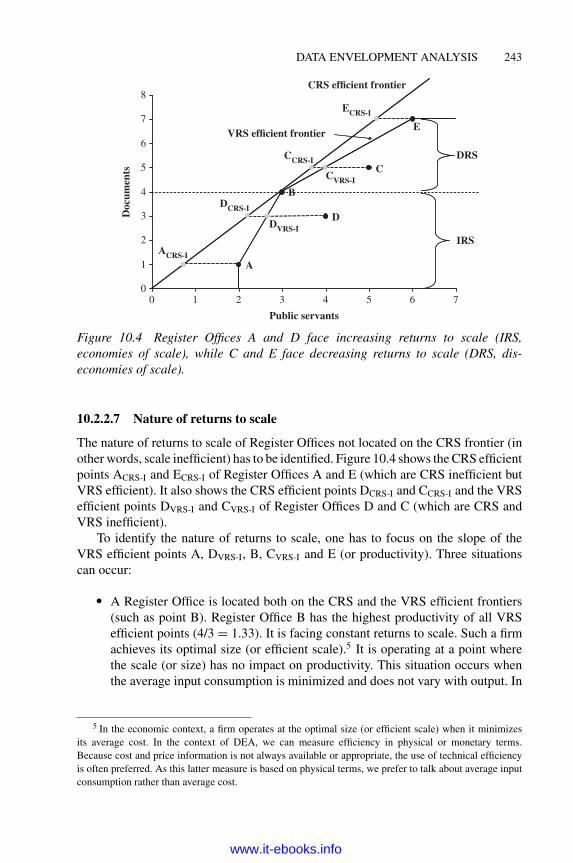
DATA ENVELOPMENT ANALYSIS 243
0
1
2
3
4
5
6
7
8
76543210
Public servants
Doc
umen
ts
A
B
D
EVRS efficient frontier
CRS efficient frontier
CDRS
IRS
DCRS-I
DVRS-I
ACRS-I
CCRS-I
CVRS-I
ECRS-I
Figure 10.4 Register Offices A and D face increasing returns to scale (IRS,economies of scale), while C and E face decreasing returns to scale (DRS, dis-economies of scale).
10.2.2.7 Nature of returns to scale
The nature of returns to scale of Register Offices not located on the CRS frontier (inother words, scale inefficient) has to be identified. Figure 10.4 shows the CRS efficientpoints ACRS-I and ECRS-I of Register Offices A and E (which are CRS inefficient butVRS efficient). It also shows the CRS efficient points DCRS-I and CCRS-I and the VRSefficient points DVRS-I and CVRS-I of Register Offices D and C (which are CRS andVRS inefficient).To identify the nature of returns to scale, one has to focus on the slope of the
VRS efficient points A, DVRS-I, B, CVRS-I and E (or productivity). Three situationscan occur:
� A Register Office is located both on the CRS and the VRS efficient frontiers(such as point B). Register Office B has the highest productivity of all VRSefficient points (4/3 = 1.33). It is facing constant returns to scale. Such a firmachieves its optimal size (or efficient scale).5 It is operating at a point wherethe scale (or size) has no impact on productivity. This situation occurs whenthe average input consumption is minimized and does not vary with output. In
5 In the economic context, a firm operates at the optimal size (or efficient scale) when it minimizesits average cost. In the context of DEA, we can measure efficiency in physical or monetary terms.Because cost and price information is not always available or appropriate, the use of technical efficiencyis often preferred. As this latter measure is based on physical terms, we prefer to talk about average inputconsumption rather than average cost.
www.it-ebooks.info

244 MULTI-CRITERIA DECISION ANALYSIS
0
1
2
3
4
5
6
7
8
76543210
Public servants
Doc
umen
ts
A
B
C
D
E
CVRS-I
DVRS-I
2.67
Figure 10.5 The ratio of productivity is increasing with the scale.
a situation of constant returns to scale, an increase in output of 1% requires aproportionate (i.e. 1%) increase in input.
� A Register Office (or the projected point of a Register Office) is located at apoint where the scale (or size) has a positive impact on productivity. PointsA and DVRS-I are in such a position (see Figure 10.5). The productivity of A(1/2 = 0.5) is less than the productivity of DVRS - I (3/2.67 = 1.125). The ratioof productivity is increasing with the scale. This situation occurs until point B,which has a productivity of 1.33. Register Offices A and D are therefore facingincreasing returns to scale (or economies of scale). In this situation, the averageinputs consumption declines whilst output rises. Register Offices A and D havenot yet reached their optimal size (or efficient scale). To improve their scaleefficiency, they have to expand their output. In a situation of economies ofscale, a variation in output of 1% results in a variation in input of less than1%. Hence, an increase in output results in a reduction of the average inputconsumption.
� A Register Office (or the projected point of a Register Office) is located at apoint where the scale (or the size) has a negative impact on productivity. PointsCVRS-I and E are in such a position (see Figure 10.6). The productivity ofCVRS-I (5/4 = 1.25) is superior to the productivity of E (7/6 = 1.17). The ratioof productivity is decreasing with the scale. This situation occurs from point B,which has a productivity of 1.33. Register Offices C and E are therefore facingdecreasing returns to scale (or diseconomies of scale). In this situation, theaverage input consumption rises whilst output rises. Register Offices C and Ehave exceeded their optimal size (or efficient scale). To improve their scale
www.it-ebooks.info

DATA ENVELOPMENT ANALYSIS 245
0
1
2
3
4
5
6
7
8
76543210
Public servants
Doc
umen
ts
A
B
C
D
E
CVRS-I
DVRS-I
C
Figure 10.6 The ratio of productivity is decreasing with the scale.
efficiency, they have to reduce their output. In a situation of diseconomies ofscale, a variation in output of 1% results in a variation in input of more than1%. Hence, a decrease in output results in a reduction of the average inputconsumption.
The specific cases of the five Register Offices are described below (seeFigure 10.4):
– A is located on the VRS frontier but not on the CRS frontier. Its inefficiency isdue to an inappropriate scale. A is facing increasing returns to scale. A variationin output of 1% results in a variation in input of less than 1%.
– D is located neither on the CRS nor on the VRS frontier. Its inefficiency isdue to an inappropriate scale and to poor management. D is facing increasingreturns to scale. A variation in output of 1% results in a variation in input ofless than 1%.
– B is located both on the CRS and on the VRS frontier. It has no inefficiency atall. B is facing constant returns to scale. A variation in output of 1% results ina variation in input of 1%.
– C is located neither on the CRS nor on the VRS frontier. Its inefficiency isdue to an inappropriate scale and to poor management. C is facing decreasingreturns to scale. A variation in output of 1% results in a variation in input ofmore than 1%.
– E is located on the VRS frontier (but not on the CRS frontier). Its inefficiency isdue to an inappropriate scale. E is evolving in a situation of decreasing returns
www.it-ebooks.info

246 MULTI-CRITERIA DECISION ANALYSIS
to scale. A variation in output of 1% results in a variation in input of morethan 1%.
10.2.2.8 Peers (or benchmarks)
DEA identifies, for each inefficient DMU, the closest efficient DMUs located on thefrontier. These efficient DMUs are called peers or benchmarks. If inefficient DMUswant to improve their performance, they have to look at the best practices developedby their respective peers.Under the CRS assumption, Register Office B is the only DMU located on the
efficient frontier. Hence it is identified as the peer for all other inefficient RegisterOffices.Figure 10.7 illustrates the peers under theVRS assumption. ThreeRegisterOffices
(A, B and E) are located on the efficient frontier. Two (C and D) are inefficient. C hastwo assigned peers, B and E, because CVRS-I, the projected point of C on the VRSfrontier, lies between these two benchmarks. D has also two assigned peers, A andB, because DVRS-I, the projected point of D on the VRS frontier, lies between thesetwo benchmarks.
0
1
2
3
4
5
6
7
8
76543210
Public servants
Doc
umen
ts
A
B
D
EVRS efficient frontier
C
DVRS-I
CVRS-I
Figure 10.7 A and B are peers of D, while B and E are peers of C.
10.2.2.9 Slacks
Particular positions located on the frontier are inefficient. Assume there is an addi-tional Register Office in our sample, F. It produces 0.5 documents with two publicservants. Figure 10.8 illustrates the efficient frontier under VRS. F is not located onthe frontier. In order to become efficient, it has first to move to point FVRS-I without slacks.
www.it-ebooks.info

DATA ENVELOPMENT ANALYSIS 247
0
1
2
3
4
5
6
7
8
76543210Public servants
Doc
umen
ts
A
B
C
E
D
F
VRS efficient frontier
SlackFVRS-I without slack
VRS efficient frontier
Figure 10.8 DEA adjusts the projected values of inefficient DMUs to take slacksinto account.
At this location, F should have an efficiency score of 100%, as it is located on thefrontier. But A, next to it on the frontier, is also 100% efficient. The differencebetween F and A is striking. With the same number of inputs (2 public servants), Fproduces 0.5 document and A produces 1 document (i.e. 0.5 more than F). Thereforepoint FVRS-I without slacks cannot be considered as 100% efficient, because it producesless output with the same amount of inputs than another Register Office (A). To geta 100% efficiency score, point FVRS-I without slacks has to move further up to point A.This additional improvement needed for a DMU to become efficient is called a slack.Indeed, every point located on the sections of the frontier which run parallel to
either the x or the y axes has to be adjusted for slacks. DEA is designed to take slacksinto account.
10.2.3 Multiple outputs and inputs
DEA allows multiple outputs and multiple inputs to be taken into account. Forexample, a shirt company uses machines, workers and cotton (three inputs) in orderto produce T-shirts, trousers and underwear (three outputs). DEA can account for allof these variables and even more. As a result, DEA goes far beyond the calculationof single productivity ratios such as the number of T-shirts produced per worker (oneoutput divided by one input).However, the total number of outputs and inputs being considered is not limitless
from a practical point of view. It depends on the number of DMUs in the data set. Ifthe number of DMUs is smaller than, roughly speaking, three times the sum of thetotal number of inputs and outputs, it is highly probable that several DMUs, if not
www.it-ebooks.info

248 MULTI-CRITERIA DECISION ANALYSIS
all, will obtain a 100% efficiency score.6 For example, a data set containing 21 shirtcompanies should be evaluated on a maximum number of seven outputs and inputs(21 divided by 3). As Cooper et al. (2006, p. 106) point out, ‘if the number of DMUs(n) is less than the combined number of inputs and outputs (m + s), a large portion ofthe DMUs will be identified as efficient and efficiency discrimination among DMUis questionable due to an inadequate number of degrees of freedom. ( . . . ) Hence,it is desirable that n exceeds m + s by several times. A rough rule of thumb inthe envelopment model is to chose n ( . . . ) equal to or greater than max{m × s,3 × (m + s)}.’DEA measures DMU efficiency based on multiple outputs and multiple inputs.
If shirt company A produces a lot of T-shirts but only a few trousers and underwear,DEA will automatically attribute a high weighting to the T-shirts variable in order toemphasize this strength. As a result, DEA automatically optimizes the weighting ofeach variable in order to present each DMU in the best possible light.Unfortunately, DEA does not work with negative or zero values for inputs and
outputs. However, zero values can be substituted with very low values such as 0.01.Adistinction has to bemade between variableswhich are under the control ofman-
agement (discretionary variables) and variables which are not (non-discretionary orenvironmental variables). Ideally, a DEAmodel will exclusively include discretionaryvariables, although someDEAmodels can also accommodate non-discretionary ones.In a second step, efficiency scores can be adjusted to account for environmental vari-ables (i.e. such variables influence the efficiency of a DMU but are not a traditionalinput and are not under the control of the manager).Moreover, variables should reflect both quantitative and qualitative characteristics
of DMUs’ resources and services. Although it may not be easy to identify andto convert qualitative characteristics into numbers, it is desirable to include suchvariables in the model in order to appropriately benchmark DMUs.
10.2.4 Types of efficiency
The notion of efficiency refers to an optimal situation; the maximum output for agiven level of input or the minimum input for a given level of output. Subject to dataavailability, several types of efficiency can be measured:
� Technical efficiency, in which both outputs and inputs are measured in physicalterms.7
6 The higher the number of inputs and outputs that are taken into consideration for a given numberof firms, the more probable it is that each firm will be the best producer of at least one of the outputs.Therefore, all firms could obtain a 100% efficiency score.
7 This chapter focuses on the measurement of technical efficiency for two main reasons. First, firmsin the public sector are often not responsible for the age pyramid of their employees; therefore takinginto account the wages of the employees (which often increase with seniority) would unfairly alter theefficiency of a firm with a greater proportion of senior employees. Second, firms in the public sector donot often produce commercial goods or services with a set price.
www.it-ebooks.info

DATA ENVELOPMENT ANALYSIS 249
� Cost efficiency: identical to technical efficiency, except that cost (or price)information about inputs is added to the model.
� Revenue efficiency: identical to technical efficiency, except that price informa-tion about outputs is added to the model.
� Profit efficiency: identical to technical efficiency, except that cost informationabout inputs and price information about outputs are added to the model.
Technical efficiency is a global measure of DMU performance. However, it doesnot indicate the source of inefficiency. This source could be twofold:
� the DMU could be poorly managed and operated;
� it could be penalized for not operating at the right scale.
Technical efficiency can be decomposed into a ‘pure’ technical efficiency measureand a scale efficiency measure to reflect these two sources of inefficiency.8
10.2.5 Managerial implications
DEA is a benchmarking technique. The efficiency scores provide information about aDMU’s capacity to improve output or input. In this sense, DEA offers strong supportto decision making. Conducting an efficiency analysis and interpreting the resultsoften raises practical questions. The following list of frequently asked questionsoffers some advice.
� Is it advisable to involve the managers of the DMUs to be benchmarked in theefficiency analysis from the beginning of the process?Yes, it is, and for two main reasons. First, managers know the processes oftheir DMUs and the data available. Therefore they are the right persons topertinently identify which inputs and outputs to integrate into the analysis.Second, managers involved from the beginning of the process are more likelyto accept the results of the analysis (rather than to reject them).
� How should one respond to managers who claim that their DMUs are differentfrom others, and therefore cannot be compared to them?Sometimes inefficiencies can be explained by indisputable environmental vari-ables. But sometimes not. Managers often justify the low efficiency scoresof their DMUs by arguing that their situations are different compared to thesituations of the other DMUs. They claim to be a ‘special case’ (and therefore
8 The firm’s management team will definitely be held responsible for the ‘pure’ technical efficiencyscore. In a situation where it does not have the discretionary power to modify the DMU’s size, it willlikely not be accountable for the scale efficiency score. However, especially in the private sector, one hasthe choice of the scale at which it operates: the management team can easily downsize the DMU and, withsome effort, upsize it also.
www.it-ebooks.info
250 MULTI-CRITERIA DECISION ANALYSIS
it is acceptable to be inefficient). Actually, the majority of DMUs could pos-sibly claim to be different as most possess something unique. However, it islikely that the difference of one DMUwill be compensated by the difference ofanother. More generally, it is up to the managers to prove that they really facea hostile environment. If they cannot prove it, management measures shouldbe taken to improve efficiency.
� Assume that a DMU obtains an efficiency score of 86.3%. Should this numberbe strictly applied?Not really, it should be interpreted more as an order of magnitude. This orderof magnitude informs managers that they have to increase their outputs or todecrease their inputs in order to become more efficient. But one should notfocus too strictly on the capacity for 13.7% improvement. Such a numbercould be interpreted by practitioners as too ‘accurate’. Therefore it is betterto consider efficiency scores as more of an objective basis to hold an opendiscussion about the way to improve DMU efficiency rather than a number tobe strictly applied.
� A DMU faces increasing returns to scale. It has economies of scale.What doesthat concretely mean from a managerial point of view?Such a DMU has not yet reached its optimal size. In order to reduce its averagetotal cost (or its average input consumption), it has to increase its size. Inpractice, this could be done either by internal growth (i.e. producing moreoutput) or by merging with another DMU which is also facing increasingreturns to scale. If, for some reason, managers cannot influence the scale of aDMU, they should not be held accountable for this source of inefficiency.
� A DMU faces decreasing returns to scale. It has diseconomies of scale. Whatdoes that concretely mean from a managerial point of view?Such a DMU is already oversized, having exceeded its optimal size. In orderto reduce its average total cost (or its average inputs consumption), it has todecrease its size. In practice, this could be done either by internal decay (i.e.producing less output) or by splitting the DMU into two separate businesses.Note that some of the production could be transferred to a DMU facing increas-ing returns to scale. If, for some reason, managers cannot influence the scaleof a DMU, they should not be held accountable for this source of inefficiency.
� Is efficiency the only criterion to assess a DMU’s performance?Not necessarily. Basically, the assessment of aDMU’s performancewill dependon themanagement objectives. Other criteria such as effectiveness or equity areoften considered alongside efficiency. If this is the case, the overall performanceshould be balanced with the various criteria.
� One DMU obtains a score of 100% but all the others in the data set obtainmuch lower scores (e.g. starting at 40% or lower). Is this realistic?It could be realistic, but the gap appears to be important. In such a case, datashould be carefully checked, and especially data of the efficient DMU. If a data
www.it-ebooks.info

DATA ENVELOPMENT ANALYSIS 251
problem is not identified, such results mean that the efficient DMU is likely tohave completely different processes than the other DMUs. It should thereforebe absolutely presented as a best practice model. However, even if they arerealistic, such results are likely to be rejected by managers whose DMUs havelow efficiency scores. These managers are likely to be discouraged because itis obviously unrealistic for them to improve their DMU’s efficiency by 60%(or more) in the short run. Therefore it is better to exclude the efficient DMUfrom the sample and to run a new model.
� Almost all the DMUs obtain an efficiency score of 100%. Does that mean thatall of them are really efficient?Yes, it could mean that all the DMUs are efficient. Such results would be great!But they are unlikely. Here, the total number of inputs and outputs is probablytoo high compared to the number of DMUs in the data set. In this case, onevariable should be excluded and a new model run. If the number of DMUsobtaining a 100% score decreases, this indicates that the number of variableswas too high compared to the number of DMUs. If not, all the DMUs are justefficient and should be congratulated!
� The model does not show any results. What does that mean?The data should be checked. This could happen when data with a value of zeroare included. Zeros should to be substituted by a very small number (0.01).
Exercise 10.1
The following multiple-choice questions test one’s knowledge on the basics of DEA.Only one answer is correct. Answers can be found on the companion website.
1. What is the main purpose of DEA?
a) DEA measures DMUs’ effectiveness
b) DEA measures DMUs’ efficiency
c) DEA measures DMUs’ profit
d) DEA measures DMUs’ productivity
2. A data set includes information about input quantity, input cost and outputquantity. Which type of efficiency cannot be measured?
a) Technical efficiency
b) Cost efficiency
c) Revenue efficiency
d) Scale efficiency
www.it-ebooks.info

252 MULTI-CRITERIA DECISION ANALYSIS
3. ‘Pure’ technical efficiency reflects:
a) A global measure of DMU performance
b) The efficiency of a DMU operating at an incorrect scale
c) A measure of profit efficiency
d) The efficiency of a poorly managed DMU
4. DMU A is inefficient. Who is (are) its peer(s)?
a) One or several DMUs whose efficiency scores are worse than A’sefficiency
b) One or severalDMUswhose efficiency scores are better thanA’s efficiency,but which are not located on the efficiency frontier
c) Any DMU located on the efficiency frontier
d) One or several specific DMUs (i.e. a subgroup of efficient DMUs) locatedon the efficiency frontier
5. A DMU faces diseconomies of scale. How can the management team improveits efficiency?
a) By merging with another DMU
b) By producing more output
c) By producing less output
d) By producing the same amount of output
6. A manager plans to measure efficiency using three inputs and two outputs.What is the minimum number of DMUs that should be included in the dataset?
a) 10
b) 6
c) 15
d) It does not matter
10.3 The DEA software
The user-friendly software packages for DEA incorporate intuitive graphical userinterfaces and automatic calculation of efficiency scores. Someof themare compatible
www.it-ebooks.info

DATA ENVELOPMENT ANALYSIS 253
with Microsoft Excel. For a survey of DEA software packages, see Barr (2004).Several software packages have been developed:
� Free packages include DEAP (Timothy Coelli, Coelli Economic ConsultingServices) andWin4DEAP (Michel Deslierres, University of Moncton), Bench-marking package in R (Peter Bogetoft, Copenhagen Business School, andLars Otto, University of Copenhagen), Efficiency Measurement System (Hol-ger Scheel, University of Dortmund) and DEA Solver Online (Andreas Kleineand Gunter Winterholer, University of Hohenheim).
� Commercial packages include DEAFrontier (Joe Zhu, Worcester Polytech-nic Institute), DEA-Solver PRO (Saitech, Inc.), PIM-DEA (Ali Emrouznejad,Aston Business School) or Frontier Analyst (Banxia Software Ltd). Zhu (2003)includes an earlier version of DEAFrontier, DEA Microsoft Excel Solver, ona CD-ROM. This software works only under Microsoft Excel 97, 2000 and2003. It allows an unlimited number of DMUs and is available at little cost.Cooper et al. (2006) include a CD-ROM with a DEA-Solver version limited at50 DMUs. It is also available at little cost.
This section focuses on the ‘twin’ DEA software packages DEAP/Win4DEAP.9
These packages centre on the basics ofDEA, are simple to use and are stable over time.They are freely available10 and come with data files as examples. As Win4DEAP istheWindows-based interface ofDEAP (which is a DOS program), the current sectionrefers only to Win4DEAP. All screenshots and icons presented in this section fromDEAP or Win4DEAP are reproduced by permission of Timothy Coelli and MichelDeslierres.The use of Win4DEAP is illustrated by a case study including a sample of 15
primary schools (see Table 10.2).
Case Study 10.2
The data used in this case study are fictitious (but are very similar to real ones).Fifteen schools produce one output (number of pupils) with three inputs (numberof full-time equivalent (FTE) teachers, number of full-time administrative staff andnumber of computers – used as a proxy for technology investment). For example,school no. 8 is teaching 512 pupils with 28.6 teachers, 1.3 administrative staff and26 computers.
9 As DEAP is a DOS program, a user-friendly Windows interface has been developed for it(Win4DEAP). These ‘twin’ software packages must both be downloaded and extracted to the same folder.Win4DEAP cannot work without DEAP.
10 DEAP Version 2.1 is available from http://www.uq.edu.au/economics/cepa/deap.htm, andWin4DEAP Version 1.1.3 from http://www8.umoncton.ca/umcm-deslierres_michel/dea/install.html.
www.it-ebooks.info

254 MULTI-CRITERIA DECISION ANALYSIS
Table 10.2 Data for Case Study 10.2.
Input Output
School FTE teachers FTE admin. staff Computers Pupils
1 40.2 2.0 37 6022 18.1 1.1 17 2693 42.5 2.1 41 6484 11.0 0.8 10 1885 24.8 1.3 22 4206 21.1 1.3 19 3747 13.5 1.0 13 2478 28.6 1.3 26 5129 23.5 1.3 22 41110 15.9 1.0 15 28511 23.2 1.3 22 39712 26.0 1.4 25 46613 11.1 0.8 11 19814 28.8 1.6 26 53015 19.7 1.3 18 357
10.3.1 Building a spreadsheet in Win4DEAP
Win4DEAP is launched by clicking on the MD icon ( ). DMUs are listed in therows, and variables (outputs and inputs) in the columns (see Figure 10.9). The openingspreadsheet contains one decision-making unit (DMU1), one output (OUT1) and oneinput (IN1) by default.To edit and name DMUs, outputs and inputs, the user must click on the row
and column labels DMU1 ( ), OUT1 ( ) and IN1 ( ), respectively. Thedialogue box shown in Figure 10.10 allows the user to (1) assign a long name anda label (maximum of eight characters) to any variable and (2) select the nature of
Figure 10.9 The opening spreadsheet contains one DMU, one output and one input.Reproduced by permission of Timothy Coelli and Michel Deslierres.
www.it-ebooks.info

DATA ENVELOPMENT ANALYSIS 255
Figure 10.10 Input and output editing. Reproduced by permission of Timothy Coelliand Michel Deslierres.
the variables (either ‘input’ or ‘output’). Finally, the user should select the with priceoption if he intends to measure cost efficiency (i.e. a price column will be added inthe spreadsheet to the variable selected).
The icons enable the user to add DMUs. The icons enable the userto add variables (inputs or outputs). The and icons are used to delete any
existing DMUs or variables. Finally, the icons allow the user to reverse theorder of appearance of DMUs (rows) or variables (columns).Data can be imported from a Microsoft Excel file into Win4DEAP by following
these steps:
1. Save theMicrosoft Excel data (only numbers, no names of DMUs or variablesshould be included) in CSV format (comma-delimited).
2. In Win4DEAP, first select the File menu, then the Import option and finallythe New data set application.
3. Select the CSV file and open it.
The data will now appear in the Win4DEAP spreadsheet, though still need to beconfigured (DMUs and variables need to be named and variables defined as inputs oroutputs).
10.3.2 Running a DEA model
To run a DEA model, the user can click on the lightning icon ( ). The windowshown in Figure 10.11 appears. This window allows a calibration of the model byfollowing steps 1–4 below:
1. Select an input or an output orientation (Orientation box).
2. Select the assumption about returns to scale (Returns to scale box). By checkingconstant, one assumes CRS; by checking variable, one assumes VRS. If one
www.it-ebooks.info

256 MULTI-CRITERIA DECISION ANALYSIS
Figure 10.11 Win4DEAP cockpit. Reproduced by permission of Timothy Coelli andMichel Deslierres.
cannot be certain that DMUs are operating at an optimal scale, running a VRSmodel is recommended.
3. Select a model (Calculate box). Three main options are available:
3.1. To calculate technical efficiency (TE) or technical (CRS), ‘pure’ (VRS)and scale efficiency (SE), check ‘DEA (multi-stage)’. Options ‘DEA (1-stage)’, ‘DEA (2-stage)’ and ‘DEA (multi-stage)’ correspond to differenttreatments of slacks. Following Coelli (1998), the multi-stage treatmentis recommended.
3.2. To calculate cost efficiency, checkDEA-COST. For this option, cost infor-mation about variables must be available and added to the spreadsheet.
3.3. To calculate technical and scale efficiency when panel data are available,check MALMQUIST. See Section 10.5.4 to learn more about this.
4. Decide how to display the results (Report box): choose between summarytables only and firm-by-firm results.
5. Click on Execute to run the model.
www.it-ebooks.info

DATA ENVELOPMENT ANALYSIS 257
Exercise 10.2
The objective of this exercise is to correctly calibrate a spreadsheet in Win4DEAPand to run a DEA model. Answers can be found on the companion website.
a) Prepare a spreadsheet in Win4DEAP including 15 DMUs, three inputs andone output. Name the DMUs ‘School 1’ to ‘School 15’. The first input is‘FTE teachers’, the second ‘FTE administrative staff’ and the third ‘Numberof computers’. The output corresponds to the number of pupils.
b) Feed the data appearing in Table 10.2 into the spreadsheet.
c) Save the file, preferably into the same folder containing DEAP/Win4DEAP(menu File/option/ Save as).
To run a DEA model in Win4DEAP, the following information is available:
� Schools are confronted with budget restrictions.
� The school system is heavily regulated.
� An obligatory school by school report is expected.
d) Calibrate the model.
e) Execute the model.
10.3.3 Interpreting results
After executing the selected model, a short notice appears with information aboutTimothy Coelli, the developer of DEAP. Results are displayed after closing thiswindow. It is recommended that first-time users spend some time navigating throughthe results file in order to become familiar with it. Some results tables are commentedon in this section. Table 10.3 contains a list of abbreviations with the main acronymsused in the results file.Figure 10.12 shows an extract from the results file and features an efficiency sum-
mary. The first column contains the 15 schools. The second one displays the constantreturns to scale technical efficiency (CRSTE) scores.11 This ‘total’ efficiency score isdecomposed into a ‘pure’ technical efficiency measure (VRSTE, third column) and
11 Note that if you had run a CRS model instead of a VRS one, you would have obtained only one typeof efficiency score in your results file (technical efficiency). Technical efficiency scores are strictly equalto the CRSTE scores obtained in the CRSTE column of the VRS model.
www.it-ebooks.info

258 MULTI-CRITERIA DECISION ANALYSIS
Table 10.3 A table of abbreviations to help with reading the results file.
Acronym Full name
DEA data envelopment analysisCRS constant returns to scaleVRS variable returns to scaleTE technical efficiencyCRSTE constant returns to scale technical efficiencyVRSTE variable returns to scale technical efficiencySE scale efficiencyIRS increasing returns to scaleDRS decreasing returns to scale
a scale efficiency measure (SE, fourth column). The last column indicates the natureof returns to scale (IRS, DRS or a dash):
� IRS means the DMU faces increasing returns to scale (economies of scale).� DRSmeans the DMU faces decreasing returns to scale (diseconomies of scale).� A dash means the DMU faces constant returns to scale; it is operating at anoptimal scale.
Figure 10.12 Technical efficiency (CRSTE) is decomposed into ‘pure’ technicalefficiency (VRSTE) and scale efficiency (SE). Reproduced by permission of TimothyCoelli and Michel Deslierres.
www.it-ebooks.info

DATA ENVELOPMENT ANALYSIS 259
On average, schools efficiency scores are:
� 94% for CRSTE; overall, schools could reduce their inputs by 6% whilsteducating the same number of pupils.
� 97.5% for VRSTE; a better school organization would be able to reduce inputconsumption by 2.5%.
� 96.4% for SE; by adjusting their scale, schools could reduce their inputs by3.6%.
All subsequent tables displayed in the results file refer to the VRSTE scores.These tables contain the following information:
� The number of the DMU under review (‘Results for firm’).
� The technical efficiency score (‘Technical efficiency’), corresponding to theVRSTE when a VRS model has been run or to the CRSTE when a CRS modelhas been run.
� The scale efficiency score (‘Scale efficiency’); note that the SE is mentionedonly when a VRS model has been run.
� The rows of the matrix represent the outputs and the inputs of the model(‘output 1’, ‘output 2’, etc., ‘input 1’, ‘input 2’, etc.)
� The first column of the matrix recalls the original values of the variables’outputs and inputs (‘original values’).
� The second column of the matrix represents the movement an inefficient DMUneeds in order to be located on the frontier (‘radial movement’).
� The third column of the matrix is the additional movement a DMU located ona segment of the frontier running parallel to the axis needs in order to becomeefficient (‘slack movement’).
� The fourth column of the matrix lists the values of the variables which enablethe DMU to be efficient (‘projected value’); these projected values take intoaccount both the radial and the slack movements.
� Finally, the listing of peers is given. Each peer is identified by a number and hasan associated weight (‘lambda weight’) representing the relative importanceof the peer.
By way of illustration, three individual school tables are specifically commentedon. School 1 (Figure 10.13) has a ‘pure’ efficiency score of 95.1% and a scaleefficiency score of 86.9%. It is facing decreasing returns to scale (DRS). By improvingthe operation of the school, 4.9% (100 – 95.1) of inputs could be saved. By adjustingthe school to its optimal size, 13.1% (100 – 86.9) of inputs could be saved.The ‘original value’ column contains the original values of the school’s vari-
ables: school 1 teaches 602 pupils with 40.2 teachers, 2 administrative staff and 37computers. However, school 1 could ‘produce’ the same quantity of output with
www.it-ebooks.info

260 MULTI-CRITERIA DECISION ANALYSIS
Figure 10.13 Results table for school 1. Reproduced by permission of Timothy Coelliand Michel Deslierres.
fewer inputs: 37.186 teachers instead of 40.2; 1.902 administrative staff instead of 2;35.185 computers instead of 37 (see the ‘projected value’ column). The decreases ininputs 2 and 3 are equal to 4.9% of the original values: (−0.098/2)100 for input 2and (−1.815/37)100 for input 3.12 The case of input 1 is slightly different: to becomeefficient, it has to decrease not only by 4.9% (minus 1.972 from the ‘radial move-ment’ column) but also by an additional 1.042 (from the ‘slack movement’ column).Overall school 1 has to decrease its first input by minus 3.014 (−1.972+ −1.042) tobecome efficient. This represents 7.5% [(−3.014/40.2)100].To improve its efficiency, school 1 has to analyze the practice of schools 3, 14
and 8, which are identified as its peers. To be a peer (or a benchmark), a DMU musthave a ‘pure’ efficiency score of 100%. The lambda weight associated with eachpeer corresponds to its relative importance among the peer group. Ideally, school 1should analyze best practice from a composite school formed by schools 3 (61.2%),14 (37.3%) and 8 (1.4%). As such a ‘virtual’ school does not exist, school 1 shouldconcentrate its best practice analysis on the peer associated with the highest lambdavalue (i.e. school 3).School 2 (Figure 10.14) has a ‘pure’ efficiency score of 83.8% and a scale
efficiency score of 96.4%. It is facing increasing returns to scale (IRS). By improvingthe operation of the school, 16.2% (100 – 83.8) of inputs could be saved. By adjustingthe school to its optimal size, 3.6% (100 – 96.4) of inputs could be saved.The ‘original value’ column contains the original values of the school’s variables:
school 2 teaches 269 pupils with 18.1 teachers, 1.1 administrative staff and 17 com-puters. However, school 2 could ‘produce’ the same quantity of output with fewerinputs: 15.163 teachers instead of 18.1; 0.922 administrative staff instead of 1.1;14.242 computers instead of 17 (see the ‘projected value’ column). The decreasesin inputs 1, 2 and 3 are equal to 16.2% of the original values (‘radial movement’
12 In aVRSmodel, the improvement in variables (decrease in inputs or increase in outputs) is calculatedaccording to the VRSTE score (only). In a CRS model, it is calculated according to the CRSTE score, orTE score, including not only the pure efficiency but also the scale efficiency.
www.it-ebooks.info

DATA ENVELOPMENT ANALYSIS 261
Figure 10.14 Results table for school 2. Reproduced by permission of Timothy Coelliand Michel Deslierres.
Figure 10.15 Results table for school 3. Reproduced by permission of Timothy Coelliand Michel Deslierres.
column). No slack movement is identified. To improve its efficiency, school shouldrefer to schools 13, 4, 14 and 8, which are identified as its peers.School 3 (Figure 10.15) has a ‘pure’ efficiency score of 100%and a scale efficiency
score of 84.2%. It is facing decreasing returns to scale (DRS). This school is wellmanaged. It cannot improve its ‘pure’ efficiency. The only capacity for improvementlies in a scale adjustment: 15.8% (100 – 84.2) of inputs could be saved.The ‘original value’ column contains the original values of the school’s variables:
school 3 teaches 648 pupils with 42.5 teachers, 2.1 administrative staff and 41 com-puters. These values are equal to the projected ones (‘pure’ efficiency = 100%). Asschool 3 is purely efficient, it acts as its own peer.
Exercise 10.3
The objective of this exercise is the interpretation of DEA results. Figure 10.16displays results for one of the 15 schools. It has been truncated in order to hide theVRS technical efficiency score. Answers can be found on the companion website.
www.it-ebooks.info

262 MULTI-CRITERIA DECISION ANALYSIS
Figure 10.16 An efficiency table helps a DMU to make decisions based on objectiveinformation. Reproduced by permission of Timothy Coelli and Michel Deslierres.
Tasks
Answer the following questions:
a) The variable returns to scale technical efficiency score has been removedfrom the table. Find a way to calculate it.
b) Assume that the ‘pure’ efficiency score is equal to 96.3%. What is the mainfeature in need of improvement: the school’s management or the school’sscale?
c) Assume that the school only has time to analyze best practice in one of itspeers. Which one should it select?
d) By how much must the school reduce input 3 in order to be located on theefficiency frontier?
10.4 In the black box of DEA
This section describes the two principal DEA models: the constant returns to scalemodel (Charnes et al. 1978) and the variable returns to scale model (Banker et al.1984). DEA is based on the earlier work of Dantzig (1951) and Farrell (1957), whoseapproach adopted an input orientation. Zhu and Cook (2008), Cooper et al. (2007)and Coelli et al. (2005) provide a comprehensive description of the methodology. By2007, Emrouznejad et al. (2008) identified more than 4000 research articles aboutDEA published in scientific journals or books.DEA is a non-parametric method. Unlike parametric methods (such as ordinary
least squares, maximum likelihood estimation or stochastic frontier analysis), inputsand outputs are used to compute, using linear programming methods, a hull repre-senting the efficiency frontier. As a result, a non-parametric method does not requirespecification of a functional form.
www.it-ebooks.info

DATA ENVELOPMENT ANALYSIS 263
10.4.1 Constant returns to scale
Charnes et al. (1978) propose a model assuming constant returns to scale (CRSmodel).13 This is appropriate when all DMUs operate at the optimal scale. Efficiencyis defined by Charnes et al. (1978, p. 430) as ‘the maximum of a ratio of weightedoutputs to weighted inputs subject to the condition that the similar ratios for everyDMU be less than or equal to unity’. Following the notation adopted by Johnes(2004), let s be the number of output, m be the number of inputs, and TEk be thetechnical efficiency of DMU k, k = 1, . . . , n, using the m inputs to produce the soutputs. Then
TEk =
s∑
r=1ur yrk
m∑
i=1vi xik
(10.1)
where yrk is the quantity of output r produced by DMU k, xik is the quantity of inputi consumed by DMU k, ur is the weight of output r, and vi is the weight of input i.The technical efficiency of DMU k is maximized under two constraints:
maximize TEk =
s∑
r=1ur yrk
m∑
i=1vi xik
(10.2)
subject to
s∑
r=1ur yr j
m∑
i=1vi xi j
≤ 1, j = 1, . . . , n, (10.3)
ur , vi > 0 ∀r = 1, . . . , s; i = 1, . . . , m. (10.4)
Inequality (10.3) says that the weights applied to outputs and inputs of DMU k cannotgenerate an efficiency score greater than 1 when applied to each DMU in the data set.Furthermore, the weights on the outputs and on the inputs are strictly positive (10.4).This linear programming problem can be dealt with by two different approaches.
In the first, the weighted sums of outputs are maximized holding inputs constant(output-oriented model). In the second, the weighted sums of inputs are minimizedholding outputs constant (input-oriented model). Note that the output and input
13 This model is also known as the Charnes, Cooper and Rhodes model (CCR model).
www.it-ebooks.info

264 MULTI-CRITERIA DECISION ANALYSIS
orientations refer to the dual equations of each model, which are not presented in thischapter. The primal equations for each model, known as the multiplier form, are asfollows. For the CRS output-oriented model we solve
minimizem∑
i=1vi xik (10.5)
subject to
m∑i=1
vi xi j −s∑
r=1ur yr j ≥ 0, j = 1, . . . , n, (10.6)
s∑r=1
ur yrk = 1, (10.7)
ur , vi > 0 ∀r = 1, . . . , s; i = 1, . . . , m. (10.8)
For the CRS input-oriented model we solve
maximizes∑
r=1ur yrk (10.9)
subject to
m∑i=1
vi xi j −s∑
r=1ur yr j ≥ 0 j = 1, . . . , n (10.10)
m∑i=1
vi xik = 1 (10.11)
ur , vi > 0 ∀r = 1, . . . , s; i = 1, . . . , m (10.12)
Using the duality in linear programming, an equivalent form, known as theenvelopment form, can be derived from this problem. It is often preferable to solve thecomputation using the envelopment form because it contains only s+m constraintsrather than n+1 constraints in the multiplier form. Dual equations can be found inJohnes (2004, p. 631).Each DMU located on the sections of the efficiency frontier running parallel to
the axes must be adjusted for output and input slacks. A formulation of the dualequations which integrates slacks can be found in Johnes (2004, p. 632). For an in-depth analysis on the treatment of slacks, and especially the multi-stagemethodology,see Coelli (1998).
Exercise 10.4
The objective of this exercise is to programm a CRS input-oriented model usingMicrosoft Excel Solver. Answers can be found on the companion website.
www.it-ebooks.info

DATA ENVELOPMENT ANALYSIS 265
Figure 10.17 AMicrosoft Excel spreadsheet ready to use with theMicrosoft ExcelSolver.
Instructions
The companion website contains a file called ‘CRS with Solver’ . It is recom-mended that users spend some time navigating around the file in order to becomefamiliar with the formulas associated with some of the cells.The spreadsheet is divided into two parts (Figure 10.17). The first part comprises
rows 2 and 3. This section enables users to successively calculate the efficiency ofthe five Register Offices (one at a time), producing two outputs (birth and marriagecertificates) with one input (public servants). The second part comprises rows 6to 10. It contains the data for Register Offices A to E (output 1 = column B,output 2 = column C, input 1 = column D, weighted sum of outputs = column E,weighted sum of the input = column F). An additional column, G, is included inthe spreadsheet. It is a working column used by Microsoft Excel Solver. Column Gcontains the weighted sum of the input minus the weighted sum of outputs.In the first part, data from each Register Office must be entered successively in
the dark grey cells (row 2, columns B, C and D). The spreadsheet already containsdata on Register Office C. The two outputs and one input of Register Office C areassigned weights in cells B3 to D3 (light grey cells). A value of 1 has been assignedto all of them in the spreadsheet (by default). The efficiency score is calculated in cellG2 (light grey cell). The value shown in this cell (700%) exceeds 100% because theSolver has not yet been run and thus the constraints of the CRSmodel do not yet apply.The Solver must first be loaded in the user’s version ofMicrosoft Excel.14
Tasks
Answer the following questions about the Solver:
a) Which cell is to be optimized?
b) In this case, do you maximize output or minimize input?
c) Which equation of the CRS model is optimized by the Solver?
14 Instructions on loading the Solver can be found in the Microsoft Excel help files.
www.it-ebooks.info

266 MULTI-CRITERIA DECISION ANALYSIS
d) Which variables can be changed in the optimization process?
e) The Solver contains two constraints. Which one corresponds to equa-tion (10.10) in the CRS model?
f) What does the other constraint show?
g) Solve the CRS model. What is the efficiency of register office C?
h) To get a 73.08% efficiency score, what are the weights associated with out-put 1, output 2 and input 1?
i) Replace the values in cells B2, C2 and D2 with the values of another RegisterOffice (A, B, D or E). What is the efficiency score?
10.4.2 Variable returns to scale
Banker et al. (1984) propose a model assuming variable returns to scale (VRSmodel).15 This is appropriate when DMUs do not operate at optimal scale. As Coelliet al. (2005, p. 172) point out, ‘the use of the CRS specification when not all DMUsare operating at the optimal scale, results in measures of TE that are confounded byscale efficiencies (SE). The use of the VRS specification permits the calculation of TEdevoid of these SE effects.’ The CRS model can be modified by relaxing the constantreturns to scale assumption. A measure of return to scale for DMU k is added in theprimal equation.The linear programming problem to be solved under VRS includes a measure of
returns to scale on the variables axis, ck, for the DMU k. The primal equations are asfollows. For the VRS output-oriented model we solve
minimizem∑
i=1vi xik − ck (10.13)
Subject to
m∑i=1
vi xi j −s∑
r=1ur yr j − ck ≥ 0, j = 1, . . . , n, (10.14)
s∑r=1
ur yrk = 1, (10.15)
ur , vi > 0 ∀r = 1, . . . , s; i = 1, . . . , m. (10.16)
15 This model is also known as the Banker, Charnes and Cooper (BCC) model.
www.it-ebooks.info

DATA ENVELOPMENT ANALYSIS 267
For the VRS input-oriented model we solve
maximizes∑
r=1ur yrk + ck (10.17)
subject to
m∑i=1
vi xi j −s∑
r=1ur yr j − ck ≥ 0, j = 1, . . . , n, (10.18)
m∑i=1
vi xik = 1, (10.19)
ur , vi > 0 ∀r = 1, . . . , s; i = 1, . . . , m. (10.20)
The reader may refer to Johnes (2004) for the dual equations (p. 634) and the dualequations with slacks (pp. 634–635).A further step needs to be taken in order to identify the nature of the returns
to scale. This relates to another model, the non-increasing returns to scale (NIRS)model, derived from the VRS model (Coelli et al. 2005). In Figure 10.18 the NIRSefficiency frontier has been added (the dotted line). This corresponds to the CRSfrontier from the origin to point B followed by the VRS frontier from point B.The nature of the scale inefficiencies for each DMU can be determined by com-paring technical efficiency scores under NIRS and VRS. If NIRS TE �= VRS TE(as for DMUs A and D), increasing returns to scale apply. If NIRS TE = VRS TE(but �= CRS TE) (as for DMUs E and C), decreasing returns to scale apply. Finally,if NIRS TE = VRS TE = CRS TE, as for DMU B, constant returns to scale apply.
CRS efficient frontier
A
D
B
C
E
VRS efficient frontier
Input
Output
D’D’’
E’
E’’
0
V
SA’
C’
T
W
U
NIRS efficient frontier
Figure 10.18 The nature of returns to scale is identified by comparing an NIRS anda VRS model.
www.it-ebooks.info

268 MULTI-CRITERIA DECISION ANALYSIS
10.5 Extensions of DEA
In this section, a selection of four extensions of DEA is briefly introduced: adjustingfor the environment, preferences (weight restrictions), sensitivity analysis and timeseries data. For a broader overview of the major developments in DEA, see Cook andSeiford (2008). For an up-to-date review of DEA, see Cooper et al. (2011).
10.5.1 Adjusting for the environment
Environmental variables influence the efficiency of DMUs but are not under thecontrol of the management team. In DEA, several methods are used to accommodatesuch variables. These include the Charnes et al. (1981) approach, the categoricalmodel (Banker and Morey 1986a) and the non-discretionary variable model derivedby Banker and Morey (1986b) (which includes the environmental variable directlyin the DEA model).The most convincing of these methods, however, is the two-stage method, the
advantages of which are described in Coelli et al. (2005, pp. 194–195) and in Pastor(2002, p. 899). The two-stage method combines a DEA model and a regressionanalysis. In the first stage, a traditional DEAmodel is conducted. This model includesonly discretionary inputs and outputs. In the second stage, the efficiency scores areregressed against the environmental (i.e. non-discretionary or exogenous) variables.Tobit regression is often used in the second stage. However, recent studies have shownthat ordinary least squares regression is sufficient to model the efficiency scores (Hoff2007) or even more appropriate than tobit (McDonald 2009).The coefficients of the environmental variables, estimated by regression, are used
to model the efficiency scores to correspond to an identical condition of environment(e.g. usually the average condition). Simar and Wilson (2007, p. 32) provide a selec-tion of studies using the two-stagemethod. Among these are applications in education(Chakraborty et al. 2001; McMillan and Datta 1998; McCarty and Yaisawarng 1993),hospitals (Burgess andWilson 1998), defence (Barros 2004), police (Carrington et al.1997), farming (Binam et al. 2003) and banking (O’Donnell and van der Westhuizen2002). Sueyoshi et al. (2010) and Sibiano and Agasisti (2012) provide more recentapplications in the manufacturing sector and education.
10.5.2 Preferences
For different reasons (e.g. the weights assigned to variables by DEA are consideredas unrealistic for some DMUs; the management team may wish to give priority tospecific variables), preferences about the relative importance of individual inputs andoutputs can be set by the decision maker. This is done by placing weight restrictionson outputs and inputs (also called multiplier restrictions). Cooper et al. (2011) andThanassoulis et al. (2004) provide a review of models regarding the use of weightsrestrictions. An earlier review can be found in Allen et al. (1997). Generally, the
www.it-ebooks.info

DATA ENVELOPMENT ANALYSIS 269
imposition of weight restrictions worsens efficiency scores. Three main approachesare identified to accommodate preferences:
� Dyson and Thanassoulis (1988) propose an approach which imposes absoluteupper and lower bounds on input and output weights. This technique is appliedin Roll et al. (1991) to highway maintenance units and in Liu (2009) to garbageclearance units.
� Charnes et al. (1990) develop the cone-ratio method. This approach imposesa set of linear restrictions that define a convex cone, corresponding to an‘admissible’ region of realistic weight restrictions. See Brockett et al. (1997)for an application to banks.
� Thompson et al. (1986, 1990) propose the assurance region method. Thisapproach is actually a special case of the cone ratio. It imposes constraints onthe relative magnitude of the weights. For example, a constraint on the ratio ofweights for inputs 1 and 2 can be included, such as L1,2 ≤ ν2
/ν1 ≤ U1,2, where
L1,2 and U1,2 are lower and upper bounds for the ratio of the weight of input 2(ν2) to the weight of input 1 (ν1). As a result, the assurance regionmethod limitsthe ‘region’ of weights to a restricted area by prohibiting large differences inthe value of those weights. An application of this model is provided by Saricaand Or (2007) in the assessment of power plants.
10.5.3 Sensitivity analysis
Cooper et al. (2006, p. 271) mention that the term ‘sensitivity’ corresponds to stabilityor robustness. For Zhu (2003, p. 217), ‘the calculated frontiers of DEA models arestable if the frontier DMUs that determine the DEA frontier remain on the frontierafter particular data perturbations are made’. Sensitivity analysis aims to identify theimpact on DMU efficiency when certain parameters are modified in the model.The first way to test the sensitivity of DEA results is to add/remove DMUs to/from
DEA models. Dusansky and Wilson (1994, 1995) and Wilson (1993, 1995) providedifferent approaches to deal with this concern. The approach of Pastor et al. (1999)allows users to identify the observations which considerably affect the efficiencyof the remaining DMUs. It also determines the statistical significance of efficiencyvariations which are due to the inclusion of a given DMU in the sample.Another way to test the sensitivity of DEA results is to modify the values of
outputs and inputs. They focus on the maximum data variations a given DMU canendure whilst maintaining its efficiency status. Approaches include:
� perturbation of a single variable of an efficient DMU (Charnes et al. 1985),data of other DMUs remaining fixed;
� simultaneous proportional data perturbation of all outputs and inputs of anefficient DMU (Charnes and Neralic 1992), data of other DMUs remainingfixed;
www.it-ebooks.info

270 MULTI-CRITERIA DECISION ANALYSIS
� simultaneous data perturbation of an efficient DMU in a situationwhere outputsand inputs can be modified individually (Seiford and Zhu 1998a; Neralic andWendell 2004), data of other DMUs remaining fixed;
� simultaneous proportional data perturbation of all outputs and inputs of allDMUs (Seiford and Zhu 1998b).
For more on sensitivity analysis, see Zhu (2001).
10.5.4 Time series data
In DEA, panel data are considered using two methods: window analysis and theMalmquist index.Window analysis, introduced by Charnes et al. (1985), examines the changes
in the efficiency scores of a set of DMUs over time. A ‘window’ of time periodsis chosen for each DMU. The same DMU is treated as if it represented a differentDMU in every time period. In this sense, window analysis can also be considered asa sensitivity analysis method. For instance, a model including n DMUs with annualdata and a chosen ‘window’ of t years will result in n × t units to be evaluated.For each DMU, t different efficiency scores will be measured. The ‘window’ is thenshifted by one period (one year in our example) and the efficiency analysis is repeated.Yue (1992) provides a didactical application of window analysis. Other applicationsinclude Yang and Chang (2009), Avkiran (2004) and Webb (2003).The Malmquist total factor productivity index was first introduced by Malmquist
(1953) before being further developed within the framework of DEA. It is used tomeasure the change in productivity over time. The Malmquist index decomposesthis productivity change into two components The first is called the ‘catch-up’;this captures the change in technical efficiency over time. The second is called the‘frontier-shift’; this captures the change in technology that occurs over time (i.e. themovement of efficiency frontiers over time). Readers may refer to Fare et al. (2011)and Tone (2004) for actual reviews. Applications of the Malmquist index can befound in Coelli and Prasada Rao (2005) and Behera et al. (2011).
References
Allen, R., Athanassopoulos, A., Dyson, R. G., and Thanassoulis, E. (1997). Weights restric-tions and value judgements in data envelopment analysis: Evolution, development and futuredirections. Annals of Operations Research, 73, 13–34.
Avkiran, N. K. (2004). Decomposing technical efficiency and window analysis. Studies inEconomics and Finance, 22(1), 61–91.
Banker, R. D., and Morey, R. C. (1986a). The use of categorical variables in data envelopmentanalysis. Management Science, 32, 1613–1627.
Banker, R. D., and Morey, R. C. (1986b). Efficiency analysis for exogenously fixed inputsand outputs. Operations Research, 34, 513–521.
Banker, R. D., Charnes, A., and Cooper, W. W. (1984). Some models for estimating tech-nical and scale inefficiencies in data envelopment analysis. Management Science, 30(9),1078–1092.
www.it-ebooks.info

DATA ENVELOPMENT ANALYSIS 271
Barr, R. (2004). DEA software tools and technology: A state-of-the-art survey. In W. W.Cooper, L. M. Seiford, and J. Zhu, Handbook on Data Envelopment Analysis (pp. 539–566). Boston: Kluwer Academic Publishers.
Barros, C. P. (2004). Measuring performance in defence-sector companies in a small NATOmember country. Journal of Economic Studies, 31, 112–128.
Behera, S. K., Faroquie, J. A., and Dash, A. P. (2011). Productivity change of coal-firedthermal power plants in India: A Malmquist index approach. IMA Journal of ManagementMathematics, 22, 387–400.
Binam, J. N., Sylla, K., Diarra, I., and Nyambi, G. (2003). Factors affecting technicalefficiency among coffee farmers in Cote d’Ivoire: Evidence from the centre west region.R&D Management, 15, 66–76.
Brockett, P. L., Charnes, A., Cooper, W. W., Huang, Z. M., and Sun, D. B. (1997).Data transformations in DEA cone ratio envelopment approaches for monitoring bankperformance. Journal of Operational Research, 98, 250–268.
Burgess, J. F., and Wilson, P. W. (1998). Variation in inefficiency among US hospitals.Canadian Journal of Operational Research and Information Processing (INFOR), 36,84–102.
Carrington, R., Puthucheary, N., Rose, D., and Yaisawarng, S. (1997). Performance mea-surement in government service provision: The case of police services in New South Wales.Journal of Productivity Analysis, 8, 415–430.
Chakraborty, K., Biswas, B., and Lewis, W. C. (2001). Measurement of technical efficiency inpublic education: A stochastic and nonstochastic production approach. Southern EconomicJournal, 67, 889–905.
Charnes, A., and Neralic, L. (1992). Sensitivity analysis in data envelopment analysis.GlasnikMatematicki, 27, 191–201.
Charnes, A., Clarke, C., Cooper, W.W., and Golany, B. (1985). A development study of DEAin measuring the effect of maintenance units in the U.S. Air Force. Annals of OperationsResearch, 2, 95–112.
Charnes, A., Cooper, W. W., and Rhodes, E. L. (1978). Measuring the efficiency of decisionmaking units. European Journal of Operational Research, 2, 429–444.
Charnes, A., Cooper, W. W., and Rhodes, E. L. (1981). Evaluating program and managerialefficiency: An application of DEA to program follow through.Management Science, 27(6),668–697.
Charnes, A., Cooper,W.W., Huang, Z.M., and Sun, D. B. (1990). Polyhedral cone-ratio DEAmodels with an illustrative application to large commercial banks. Journal of Econometrics,46, 73–91.
Coelli, T. J. (1998). A multi-stage methodology for the solution of oriented DEA models.Operations Research Letters, 23, 143–149.
Coelli, T. J., and Perelman, S. (1996). Efficiency measurement, multiple-output technologiesand distance functions: With application to European railways. Center of Research in PublicEconomics and Population Economics Discussion Paper 96/05.
Coelli, T. J., and Perelman, S. (1999). A comparison of parametric and non-parametricdistance functions:With application to European railways.European Journal of OperationalResearch, 117(2), 326–339.
Coelli, T. J., and Prasada Rao, D. S. (2005). Total factor productivity growth in agriculture:A Malmquist index analysis of 93 countries, 1980–2000. Agricultural Economics, 32,115–134.
www.it-ebooks.info

272 MULTI-CRITERIA DECISION ANALYSIS
Coelli, T. J., Prasada Rao, D. S., O’Donnell, C. J., and Battese, G. E. (2005). An Introductionto Efficiency and Productivity Analysis. New York: Springer-Verlag.
Cook, W. D., and Seiford, L. M. (2008). Data envelopment analysis (DEA) – Thirty years on.European Journal of Operational Research, 192, 1–17.
Cooper, W.W., Ruiz, J. L., and Sirvent, I. (2011). Choices and uses of DEAweights. InW.W.Cooper, L. M. Seiford, and J. Zhu,Handbook on Data Envelopment Analysis (pp. 93–126).New York: Springer-Verlag.
Cooper, W. W., Seiford, L. M., and Tone, K. (2006). Introduction to Data EnvelopmentAnalysis and its Uses. New York: Springer-Verlag.
Cooper, W. W., Seiford, L. M., and Tone, K. (2007). Data Envelopment Analysis: A compre-hensive Text with Models, Applications, References and DEA-Software.NewYork: Springer-Verlag.
Dantzig, G. B. (1951). Maximization of a linear function of variables subject to linear inequal-ities. In T. C. Koopmans, Activity Analysis of Production and Allocation (pp. 339–347).New York: John Wiley & Sons, Inc.
Dusansky, R., and Wilson, P. W. (1994). Measuring efficieny in the care of developmentallydisabled. Review of Economics and Statistics, 76, 340–345.
Dusansky, R., and Wilson, P. W. (1995). On the relative efficiency of alternative modes ofproducing public sector output: The case of the developmentally disabled.European Journalof Operational Research, 80(3), 608–618.
Dyson, R. G., and Thanassoulis, E. (1988). Reducing weight flexibility in DEA. Journal ofthe Operational Research Society, 39(6), 563–576.
Emrouznejad, A., Parker, B. R., and Tavares, G. (2008). Evaluation of research in efficiencyand productivity: A survey and analysis of the first 30 years of scholarly literature in DEA.Socio-Economic Planning Sciences, 42, 151–157.
Fare, R., Grosskopf, S., and Margaritis, D. (2011). Malmquist productivity indexes and DEA.In W. W. Cooper, L. M. Seiford, and J. Zhu, Handbook on Data Envelopment Analysis(pp. 127–150). New York: Springer-Verlag.
Farrell, M. J. (1957). The measurement of productive efficiency. Journal of Royal StatisticalSociety, Series A, 120(3), 253–281.
Giannoulis, C., and Ishizaka, A. (2010). A web-based decision support system with ELEC-TRE III for a personalized ranking of British universities. Decision Support Systems, 48,488–497.
Hoff, A. (2007). Second stage DEA: Comparison of approaches for modeling the DEA score.European Journal of Operational Research, 181, 425–435.
Johnes, J. (2004). Efficiency measurement. In G. Johnes, and J. Johnes, International Hand-book on the Economics of Education (pp. 613–742). Cheltenham: Edward Elgar.
Liu, C.-C. (2009). A study of optimal weights restriction in data envelopment analysis. AppliedEconomics, 41(14), 1785–1790.
Malmquist, S. (1953). Index numbers and indifferences surfaces. Trabajos de Estatıstica, 4,209–242.
McCarty, T. A., and Yaisawarng, S. (1993). Technical efficiency in New Jersey school districts.In H. O. Fried, C. A. Lovell, and S. S. Schmidt, The Measurement of Productive Efficiency:Techniques and Applications (pp. 271–287). New York: Oxford University Press.
McDonald, J. (2009). Using least squares and tobit in second stage DEA efficiency analyses.European Journal of Operational Research, 197, 792–798.
www.it-ebooks.info

DATA ENVELOPMENT ANALYSIS 273
McMillan, M. L., and Datta, D. (1998). The relative efficiencies of Canadian universities: ADEA perspective. Canadian Public Policy – Analyse de Politiques, 24, 485–511.
Neralic, L. (2004). Preservation of efficiency and inefficiency classification in data envelopmentanalysis. Mathematical Communications, 9, 51–62.
O’Donnell, C. J., and van der Westhuizen, G. (2002). Regional comparisons of bankingperformance in South Africa. South African Journal of Economics, 70, 485–518.
Pastor, J. M. (2002). Credit risk and efficiency in the European banking system: A three-stageanalysis. Applied Financial Economics, 12, 895–911.
Pastor, J. M., Ruiz, J. L., and Sirvent, I. (1999). A statistical test for detecting influentialobservations in DEA. European Journal of Operational Research, 115, 542–554.
Roll, Y., Cook, W. D., and Golany, B. (1991). Controlling factor weights in data envelopmentanalysis. IEE Transactions, 23(1), 2–9.
Sarica, K., and Or, I. (2007). Efficiency assessment of Turkish power plants using dataenvelopment analysis. Energy, 32, 1484–1499.
Seiford, L. M., and Zhu, J. (1998a). Stability regions for maintaining efficiency in dataenvelopment analysis. European Journal of Operational Research, 108(1), 127–139.
Seiford, L. M., and Zhu, J. (1998b). Sensitivity analysis of DEA models for simultaneouschanges in all the data. Journal of the Operational Research Society, 49, 1060–1071.
Sibiano, P., and Agasisti, T. (2012). Efficiency and heterogeneity of public spending ineducation among Italian regions. Journal of Public Affairs, to appear.
Simar, L., and Wilson, P. W. (2007). Estimation and inference in two-stage, semi-parametricmodels of production processes. Journal of Econometrics, 136, 31–64.
Sueyoshi, T., Goto, M., and Omi, Y. (2010). Corporate governance and firm performance:Evidence from Japanese manufacturing industries after the lost decade. European Journalof Operational Research, 203, 724–736.
Thanassoulis, E., Portela, M. C. S., and Allen, R. (2004). Incorporating value judgments inDEA. In W. W. Cooper, L. W. Seiford and J. Zhu (Eds.), Handbook on Data EnvelopmentAnalysis (pp. 99–138). Boston: Kluwer Academic Publishers.
Thanassoulis, E., Portela, M. C. S., and Despic, O. (2008). Data Envelopment Analysis: TheMathematical Programming Approach to Efficiency Analysis. In H. O. Fried, C. A. Lovell,and S. S. Schmidt, The Measurement of Productive Efficiency and Productivity Growth(pp. 251–420). New York: Oxford University Press.
Thomson, R. G., Langemeier, L. N., Lee, C., Lee, E., Thrall, R. M., and Smith, B. A.(1990). The role of multiplier bounds in efficiency analysis with application to Kansasfarming. Journal of Econometrics, 46, 93–108.
Thomson, R. G., Singleton Jr., F. D., Thrall, R. M., and Smith, B. A. (1986). Comparativesite evaluations for locating a high-energy physics lab in Texas. Interfaces, 16(6), 35–49.
Tone,K. (2004).Malmquist productivity index –Efficiency change over time. InW.W. Cooper,L.M. Seiford, and J. Zhu,Handbook on Data Envelopment Analysis (pp. 203–227). Boston:Kluwer Academic Publishers.
Webb, R. (2003). Level of efficiency in UK retail banks: a DEAwindow analysis. InternationalJournal of the Economics of Business, 10(3), 305–322.
Wilson, P. W. (1995). Detecting influential observations in data envelopment analysis. Journalof Productivity Analysis, 6, 27–45.
Wilson, P. W. (1993). Detecting outliers in deterministic non-parametric frontier models withmultiple outputs. Journal of Business and Economic Statistics, 11, 319–323.
www.it-ebooks.info

274 MULTI-CRITERIA DECISION ANALYSIS
Yang, H.-H., and Chang, C.-Y. (2009). Using DEA window analysis to measure efficienciesof Taiwan’s integrated telecommunication firms. Telecommunications Policy, 33, 98–108.
Yue, P. (1992). Data envelopment analysis and commercial bank performance: A primer withapplications to Missouri banks. Federal Reserve Bank of St Louis Review, 74, 31–45.
Zhu, J. (2003).Quantitative Models for Performane Evaluation and Benchmarking.NewYork:Springer-Verlag.
Zhu, J. (2001). Super-efficiency andDEAsensitivity analysis.European Journal of OperationalResearch, 129(2), 443–455.
Zhu, J., and Cook,W.D. (2008).Data Envelopment Analysis: Modeling Operational Processesand Measuring Productivity. Seattle: CreateSpace.
www.it-ebooks.info

Part IV
INTEGRATED SYSTEMS
Multi-Criteria Decision Analysis: Methods and Software, First Edition. Alessio Ishizaka and Philippe Nemery.© 2013 John Wiley & Sons, Ltd. Published 2013 by John Wiley & Sons, Ltd.
www.it-ebooks.info

11
Multi-method platforms
11.1 Introduction
The multi-criteria decision aid literature is overloaded with various different methodsand algorithms, with the aim of helping a decision maker faced with a complex, real-world decision problem. These methods differ in the type of problem they tackle,the underlying philosophy on which they are based, the assumptions they rely onand the input information they require, etc. Nevertheless the methods share somecommonalities. Most of the well-known and commonly used methods have beenimplemented in different software packages, as the contents of this book attest.
It might be difficult for a decision maker to choose the most appropriate softwarefor solving the decision problem. Furthermore, the decision problems change andevolve over time and might require the method to be changed for a more appropriateone. From a practical point of view, using different methods for the same problem (ifthe input conditions allow and assumptions are valid) may strengthen confidence inthe results.
Two main projects have arisen over the last decade in order to combine severalmethods and to strengthen interoperability: Decision Deck and DECERNS. Althoughthese two projects differ considerably in their approach, they both enable the user totest different methods in one package.
In this chapter Decision Deck is briefly described and a user-oriented descriptionof DECERNS is put forward. As our aim is to describe methods and software packagesthat require no a priori technical knowledge and can be used by beginners andexperienced practitioners alike, we describe the DECERNS project in more detail. TheDECERNS project includes several methods that have been described in the previouschapters of this book. It also contains an integrated Geographical Information Systemthat can be useful if the decision maker is dealing with with spatial alternatives.
Multi-Criteria Decision Analysis: Methods and Software, First Edition. Alessio Ishizaka and Philippe Nemery.© 2013 John Wiley & Sons, Ltd. Published 2013 by John Wiley & Sons, Ltd.
www.it-ebooks.info

278 MULTI-CRITERIA DECISION ANALYSIS
11.2 Decision Deck
The aim of Decision Deck (http://www.decision-deck.org/) is ‘collaboratively devel-oping Open Source software tools implementing MultiCriteria Decision Aid (MCDA)techniques which are meant to support complex decision aid processes’. DecisionDeck is a collaborative project involving 18 researchers (from several European coun-tries such as France, Spain, the Netherlands, Luxembourg and Belgium) and is ledby an executive committee.
Decision Desktop, also called D2, which is a rich open source Java client, includesthe following MCDA methods:
� the IRIS sorting method (Dias and Mousseau 2003);
� the RUBIS and VIP choice method (Bisdorff et al. 2008; Dias and Climaco,2000);
� the UTA-GMS/GRIP ranking method (Greco et al. 2008; Figueira et al. 2009);see Chapter 4.
Furthermore, Decision Deck proposes a standardized XML schema to representMCDA objects and data structures. This XML schema permits better interoperabilitybetween software packages. Based on this schema, the user has access to XMDAweb services, enabling the distribution of the RUBIS Python solver and the KappalabR-script (Grabisch et al. 2012).
The Decision Deck project is also active in the development of the so-called Divizopen source Java client and server (Veneziano et al. 2009) which is for designing,executing and sharing several MCDA methods by composition of web services,workflow management and deployment.
It must be stressed that the main feature of these software solutions is that theyare interoperable in order to create a coherent ecosystem.
Decision Deck is targeted at practitioners, teachers and researchers who want tocompare and test different methods. However, to use it effectively requires a strongtechnical and theoretical background.
11.3 DECERNS
The aim of DECERNS (which stands for Decision Evaluation for Complex Environ-mental Risk Network Systems) is ‘the development of an integrated, user-intuitivesoftware platform which can use diverse data sources including spatial and tempo-ral data, value and judgment criteria and quantitative environmental models output,to provide a comprehensive risk management tool’ (Grebenkov et al. 2007). TheDECERNS project is thus orientated ‘to the creation of web spatial decision supportsystems, including web-based and desktop software tools for multicriteria decisionanalysis on land use planning, risk management, and, in general, on a wide range ofproblems on (multicriteria) analysis of alternatives’ (Yatsalo et al. 2010a).
www.it-ebooks.info

MULTI-METHOD PLATFORMS 279
The DECERNS platform, illustrated in this section, provides the user with all thefunctionalities and tools for data input, scoring, weighting and sensitivity analysis,etc. for several MCDA methods. However, it does not include all method-specificaspects, for example the Gaia map, preference matrix or uni-criterion flows of thePROMETHEE method. DECERNS, to the best of our knowledge, is the only platformthat easily permits the use and comparison of different methods on the same data set.The user can define the weights for each method by choosing from various weightelicitation methods; for example, Ishizaka et al. (2013) have compared the use ofthree multi-criteria methods, namely the weighted sum, PROMETHEE and TOPSIS,for site selection for the construction of a casino in the greater London area.
DECERNS was an internationally collaborative project carried out by ObninskState Technical University of Nuclear Power Engineering (Russia), Joint Institutefor Power and Nuclear Research (Belarus), Brookhaven National Laboratory (NewYork) and Cambridge Environmental Inc. (Massachusetts). It was funded by theUnited States Department of Energy (DoE) Initiatives for Proliferation Prevention(IPP) programme, where its development was based on the previous web version ofPRANA Decision Support System (Yatsalo 2007).
Now a family of DECERNS systems/software tools have been developed andare supported by the Decision Evaluation & Software Development company(DeE&Soft); see http://deesoft.ru/lang/en.
The DECERNS Spatial Decision Support System (SDSS) has been developedon the basis of Java technologies (Java EE5) as a distributed application constructedon the information–application–client layer architecture. DECERNS SDSS is thusa client–server application. The client tier that constitutes the user interaction pointwith the system is presented by a set of html pages, Java applets and JavaScriptmodules (Yatsalo et al. 2010a). This means that DECERNS SDSS is a web application(provided with an advanced security access control) relying on different componentsthat can be (re)used in different applications as explained below. For applicationsand case studies, see Yatsalo et al. (2010a, 2010b, 2011b), Sullivan et al. (2009) andGritsyuk et al. (2011).
The DECERNS platform contains three core modules:
� Geographical Information System (GIS) module;
� Multi-Criteria Decision Aid (MCDA) module;
� Group Decision Support System (GDSS) module.
These modules are fully integrated but can work independently and are brieflydescribed in the following sections.
11.3.1 The GIS module
The GIS module provides ‘map functionalities’ that allow a user-friendly, two-dimensional visualization of spatial data and spatial data analysis (Yatsalo et al.2010a):
www.it-ebooks.info
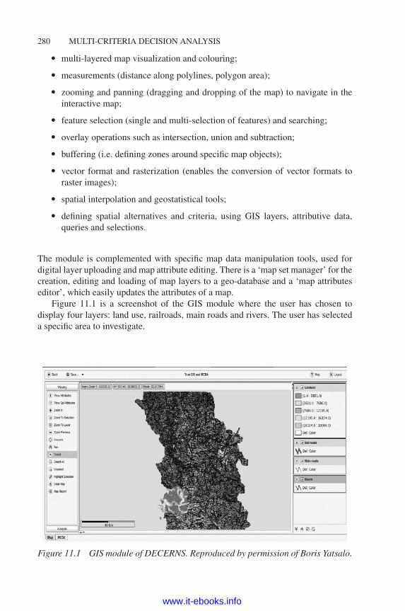
280 MULTI-CRITERIA DECISION ANALYSIS
� multi-layered map visualization and colouring;
� measurements (distance along polylines, polygon area);
� zooming and panning (dragging and dropping of the map) to navigate in theinteractive map;
� feature selection (single and multi-selection of features) and searching;
� overlay operations such as intersection, union and subtraction;
� buffering (i.e. defining zones around specific map objects);
� vector format and rasterization (enables the conversion of vector formats toraster images);
� spatial interpolation and geostatistical tools;
� defining spatial alternatives and criteria, using GIS layers, attributive data,queries and selections.
The module is complemented with specific map data manipulation tools, used fordigital layer uploading and map attribute editing. There is a ‘map set manager’ for thecreation, editing and loading of map layers to a geo-database and a ‘map attributeseditor’, which easily updates the attributes of a map.
Figure 11.1 is a screenshot of the GIS module where the user has chosen todisplay four layers: land use, railroads, main roads and rivers. The user has selecteda specific area to investigate.
Figure 11.1 GIS module of DECERNS. Reproduced by permission of Boris Yatsalo.
www.it-ebooks.info

MULTI-METHOD PLATFORMS 281
11.3.2 The MCDA module
The MCDA module aims to structure a decision problem (i.e. define the criteria andalternatives), evaluate the alternatives and weight the criteria, thereby solving theproblem. First, the decision maker has to choose from the following decision aidmethods:
� ranking methods:
◦ MAUT (see Chapter 4)
◦ MAVT (multi-attribute value theory)
◦ AHP (see Chapter 2)
◦ PROMETHEE (see Chapter 6)
◦ TOPSIS (see Chapter 8)
� sorting method:
◦ FlowSort (see Chapter 6.5.2).
It is not necessary for the input data to be precisely defined. Probabilistic distribu-tions and ‘fuzzy’ numbers can be used in the case of uncertainty. Different graphicaland tabular tools are implemented to introduce probabilistic input/output data (i.e.density distributions). The weights and the evaluations can be roughly defined bymeans of distributions such as the normal, uniform, log-normal and delta distribu-tions. This is illustrated in Figure 11.2. Different graphical and tabular tools are also
Figure 11.2 The probability menu in DECERNS. Reproduced by permission of BorisYatsalo.
www.it-ebooks.info
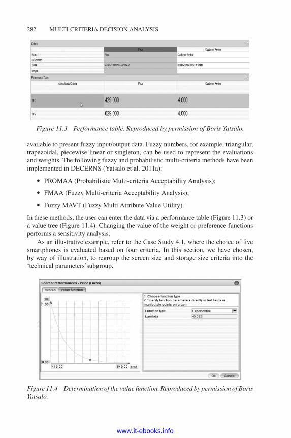
282 MULTI-CRITERIA DECISION ANALYSIS
Figure 11.3 Performance table. Reproduced by permission of Boris Yatsalo.
available to present fuzzy input/output data. Fuzzy numbers, for example, triangular,trapezoidal, piecewise linear or singleton, can be used to represent the evaluationsand weights. The following fuzzy and probabilistic multi-criteria methods have beenimplemented in DECERNS (Yatsalo et al. 2011a):
� PROMAA (Probabilistic Multi-criteria Acceptability Analysis);
� FMAA (Fuzzy Multi-criteria Acceptability Analysis);
� Fuzzy MAVT (Fuzzy Multi Attribute Value Utility).
In these methods, the user can enter the data via a performance table (Figure 11.3) ora value tree (Figure 11.4). Changing the value of the weight or preference functionsperforms a sensitivity analysis.
As an illustrative example, refer to the Case Study 4.1, where the choice of fivesmartphones is evaluated based on four criteria. In this section, we have chosen,by way of illustration, to regroup the screen size and storage size criteria into the‘technical parameters’subgroup.
Figure 11.4 Determination of the value function. Reproduced by permission of BorisYatsalo.
www.it-ebooks.info

MULTI-METHOD PLATFORMS 283
Figure 11.5 Tree structure of a decision problem in DECERNS, showing the Directweighting dialogue as well as the performances of SP5. Reproduced by permissionof Boris Yatsalo.
As illustrated in Figure 11.5, the tree structure gives a user-friendly representationof the decision problem. The task (choice of a smartphone), criteria (price, customerreviews, etc.) and alternatives (SP1, SP2, etc.) can be viewed in this tree.
The dialogue boxes have been added to allow the introduction of direct weightsand performance of alternatives. There is another view of the decision problem, whichdisplays the performance table as in Figure 11.3.
Figure 11.5 shows that the weight determination can be achieved in various ways.The user can choose from:
� direct weight determination;
� the SWING method;
� ranking of the weights;
� rating of the weights;
� pairwise comparison of the weights as with the AHP method (see Chapter 2).
The preference value functions of the criteria can be ‘drawn’ easily accordingto the decision maker’s preference (see Figure 11.4). The user has a choice betweenpiecewise linear functions and exponential functions. The final results are illustratedin Figure 11.6.
www.it-ebooks.info

284 MULTI-CRITERIA DECISION ANALYSIS
Figure 11.6 Results according to the MAUT method. Reproduced by permission ofBoris Yatsalo.
The user can perform two different types of sensitivity analysis by:
� modifying the weights of the criteria or displaying the ‘Line weights’ represen-tation which illustrates which weight value in a specifically chosen criterionchanges the ranking (Figure 11.7);
� modifying the shape of the utility function of a criterion and analysing thecorresponding change in the ranking (Figure 11.8).
The user can easily change the decision aid method, for example, when changingthe decision aid in the TOPSIS method, the user needs to redefine the model-specificparameters, such as the preference functions in PROMETHEE. Figure 11.9 representsthe results obtained with the TOPSIS method while defining identical weight values(the user needs to consider the meaning of the parameters for each method as theyare often different).
Figure 11.10 shows the sensitivity analysis of the result obtained with the TOPSISmethod when changing the weight values. This differs significantly from the analysisobtained with the MAUT method.
11.3.3 The GDSS module
The DECERNS project has a specific GDSS module which permits the creationand administration of online surveys. The results of these surveys are automaticallycollected and analysed. This feature is essential when alternatives have to be assessedby various decision makers.
www.it-ebooks.info

MULTI-METHOD PLATFORMS 285
Figure 11.7 Criterion analysis window. Reproduced by permission of Boris Yatsalo.
Figure 11.8 Value function analysis window. Reproduced by permission of BorisYatsalo.
www.it-ebooks.info

286 MULTI-CRITERIA DECISION ANALYSIS
Figure 11.9 Representation of the results obtained with the TOPSIS method. Repro-duced by permission of Boris Yatsalo.
11.3.4 Integration
As mentioned in the introduction, all modules are fully integrated. This implies that theuser can define areas in a map and define them as alternatives of the decision problem.The alternatives from a map can automatically be transferred into the performancetable and vice versa. This integration is a strong advantage of the decision supportsystem.
Figure 11.10 The criterion analysis window for the TOPSIS results.
www.it-ebooks.info
MULTI-METHOD PLATFORMS 287
References
Bisdorff, R., Meyer, P., and Roubens, M. (2008). Rubis: A bipolar-valued outranking methodfor the choice problem. 4OR, 6(2), 143–165.
Dias, L., and Climaco, J. (2000). Additive aggregation with variable interdependent parame-ters: the VIP analysis software. Journal of the Operational Research Society, 51, 1070–1082.
Dias, L., and Mousseau, V. (2003). IRIS: A DSS for multiple criteria sorting problems. Journalof Multi-Criteria Decision Analysis, 12(4–5), 285–298.
Figueira, J., Greco, S., and Slowinski, R. (2009). Building a set of additive value functionsrepresenting a reference preorder and intensities of preference: GRIP method. EuropeanJournal of Operational Research, 195(2), 460–486.
Grabisch, M., Meyer, P., and Kojadinovic, I. (2012). Kappalab R-Script. Retrieved June 2012,from Kappalab: http://cran.r-project.org/web/packages/kappalab/kappalab.pdf
Grebenkov, A., Yatsalo, B., Sullivan, T., and Linkov, I. (2007). DECERNS: Methodology andSoftware for Risk-Based Land Use Planning and Decision Support (in EnviroInfo). Aachen:Shaker Verlag.
Greco, S., Mousseau, V., and Slowinski, R. (2008). Ordinal regression revisted: Multiplecriteria ranking using a set of additive value functions. European Journal of OperationalResearch, 191, 416–436.
Gritsyuk, S., Yatsalo, B., Babutski, A., Mirzeabasov, O., and Didenko, V. (2011). Multicriteriadecision analysis with the use of DECERNS DSS. MCDM Conference 2011.
Ishizaka, A., Nemery, P., and Lidouh, K. (2013). Location selection for the construction of acasino in the greater London region: A triple multi-criteria approach. Tourism Management,34(1), 211–220.
Sullivan, T., Yatsalo, B., Grebenkov, A., and Linkov, I. (2009). Decision Evaluation forComplex Risk Network Systems (Decerns) software tool. In A. Marcomini, G. W. Suter II,and A Critto (eds), Decision Support Systems for Risk-Based Management of ContaminatedSites. New York: Springer Science + Business Media.
Veneziano, T., Bigaret, S., and Meyer, P. (2009). Diviz: An MCDA components workflowexecution engine. Euro XXIII: 23td Euroepan Conference on Operational Research. Bonn,Germany.
Yatsalo, B. (2007). Decision support system for risk based land management and rehabilita-tion of radioactively contaminated territories: PRANA approach. International Journal ofEmergency Management, 4(3), 504–523.
Yatsalo, B., Didenko, V., Tkachuk, A., and Gritsyuk, S. (2010a). Application to land useplanning. International Journal of Information Systems and Social Change, 1(1), 11–30.
Yatsalo, B., Gritsyuk, S., Didenko, V., Vasilevskaya, M., Mirzeabasov, O., and Babutski, A.(2010b). Land-use planning and risk management with the use of web-based multi-criteriaspatial decision support system (DECERNS). 25th Mini Euro-Conference: Uncertainty andRobustness in Planning and Decision Making. Coimbra, Portugal.
Yatsalo, B., Gritsyuk, S., Mirzeabasov, O., and Vasilvskaya, M. (2011a). Uncertaintytreatment within multicriteria decision analysis with the use of acceptability concept. Controlof Big Systems, 32, 5–30.
Yatsalo, B., Sullivan, T., Didenko, V., and Linkov, I. (2011b). Environmental risk managementfor radiological accidents: Integrating risk assessment and decision analysis for remediationat different spatial scales. Integrated Environmental Assessment and Management, 7(3),393–395.
www.it-ebooks.info

Appendix
Linear optimization
A.1 Problem modelling
Linear optimization (or linear programming) is a mathematical method for determin-ing the value of decision variables in order to obtain the best outcome (e.g. the highestprofit or lowest cost) under given constraints. We will illustrate the method with atransportation problem described in Case Study A.1.
Case study A.1
A company has a transportation problem. It needs to transfer two products, nailsand screws, to a warehouse. The company owns a small van, which can transporta maximum of 5 tonnes in weight and 10 m3 in volume of goods. The transportneeds to take into account the following data: 1 tonne of nails has a volume of1 m3 and brings in a revenue of £200; 1 tonne of screws has a volume of 5 m3 andbrings in a revenue of £300. What quantity of each product should the companytransport in order to maximize the benefit?
The solution to a linear programming problem is achieved in four steps:
1. Identify the objective of the problem.The objective of the problem is to either maximize (e.g. profit) or minimize(e.g. costs) a function. In Case Study A.1, the objective is to maximize thebenefit.
2. Indentify the decision variablesDecision variables are independent variables that are changed until the desiredbenefit is obtained (i.e. maximum or minimum). In Case Study A.1, the weight
Multi-Criteria Decision Analysis: Methods and Software, First Edition. Alessio Ishizaka and Philippe Nemery.© 2013 John Wiley & Sons, Ltd. Published 2013 by John Wiley & Sons, Ltd.
www.it-ebooks.info

APPENDIX: LINEAR OPTIMIZATION 289
of the nails and screws should be adjusted to maximize the benefit under thegiven constraints.
3. Identify the objective functionThe objective function describes a linear relation between the decision vari-ables and the objective of the problem. InCase StudyA.1, we need tomaximizethe weight of nails (x) and screws (y) sold in order to maximize the profit:
max 200x + 300y.
4. Identify the constraintsThe constraints define the limit of the decision variables. They are also linear.In Case Study A.1, the constraints are set by the capacity of the van:
x + y ≤ 5 (constraint on weight)x + 5y ≤ 10 (constraint on volume)x, y ≥ 0 (non-negative constraint)
A.2 Graphical solution
If the problem only contains two decision variables, a solution can be found graphi-cally. Each axis represents a decision variable and the straight lines of the constraints,obtained by replacing the inequality with equality, are sketched:
y = −x + 5 (constraint on weight)y = (−x + 10)/5 (constraint on volume)
These lines determine the feasible region, which is the collection of all the pointsthat satisfy all constraints. The direction of the arrows (left or right of the lines) isdecided by testing one point, generally the origin. If this point satisfies the constraint,then the arrow points in that direction. For example, if we introduce the origin (0,0)in the constraint weight (0 ≤ 5) and volume (0 ≤ 10), both constraints are satisfied.Finally, the coordinates of each corner point should be substituted into the objec-
tive function to determine the optimal value because the solution is necessarily onone of the corner point. In Case Study A.1, the optimal value is 3.75 tonnes of nailsand 1.25 tonnes of screws (Figure A.1).For an analytic solution, where there are more than two decision variables, the
simplex algorithm is used.
A.3 Solution with Microsoft Excel
In Figure A.2 the problem is modelled in Microsoft Excel. The first three lines arethe given data. The variable parameters (Figure A.2) have to be entered in Solver(Figure A.3):
www.it-ebooks.info

290 APPENDIX: LINEAR OPTIMIZATION
y (screws)x + y ≤ 5 (weight)
x + 5y ≤ 10 (volume)
max z = 200x + 300y
optimum
(3.75;1.25)
x (nails)95
5
Figure A.1 Graphical solution.
� The objective of the problem to be maximized is given by the benefit in cellD12.
� The decision variables are set in cells B6 and B7.
� The constraint on weight is given by cell B12 (which must be less than or equalto B14).
� The constraint on volume is given by cell C12 (which must be less than orequal to C14).
The Solver changes the initial data in B6 and B7 until the maximum in D12 isobtained.
Figure A.2 Modelling of the problem inMicrosoft Excel.
www.it-ebooks.info

APPENDIX: LINEAR OPTIMIZATION 291
Figure A.3 Solver parameters.
Exercise A.1
Here you will learn to use theMicrosoft Excel Solver.
Learning Outcomes
� Understand the modelling of a linear optimization problem
� Understand the configuration of Microsoft Excel Solver
Tasks
Open the file Transport.xls. It contains a spreadsheet with the modelling of theproblem of the Case Study A.1.Answer the following questions:
a) In the spreadsheet, find the objective of the problem, the decision variablesand the constraints. (Read the comments in the red square in case of difficulty.)
b) Open the Solver. What is entered in the set target cell? What is entered inthe ‘By Changing Cells’ box? What is entered in the ‘Subject to Constraints’box?
www.it-ebooks.info
Index
123AHP, 20
additive aggregation, 39additive model, 84AHPSort, 53analytic hierarchy process ordering, 44anti-ideal solution, 215assignment, 207
benchmarks, 246benefit hierarchy, 41
central profile, 51, 52, 173Chebyshev goal programming, 232choice problem, 3, 181ChoiceResults, 20classification problems, 1closed system, 39closeness coefficient, 219cluster, 59clusters and pivots method, 51comparative judgment, 118comparison matrix, 18comparisonsmissing, 45
compensation, 180complete ranking, 145, 166concordance, 185concordance index, 195Condorcet paradox, 203
consensus vote, 44consistency, 19, 33, 133consistency ratio, 23constant return to scale, 266correlated criteria, 59correlation, 146cost efficiency, 249cost hierarchy, 41credibility index, 195criteria priorities, 16Criterium, 20CRS efficient frontier, 239CRS model, 237
DEAP, 253DECERNS, 286Decision Deck, 278Decision Lens, 20, 68decision stick, 147, 157, 168description problem, 4design problem, 4deviational variable, 223direct rating, 21discordance index, 196diseconomies of scale, 244, 250distillation, 187distillation, 200distributive mode, 39distributive normalisation, 217DMU, 236, 247
Multi-Criteria Decision Analysis: Methods and Software, First Edition. Alessio Ishizaka and Philippe Nemery.© 2013 John Wiley & Sons, Ltd. Published 2013 by John Wiley & Sons, Ltd.
www.it-ebooks.info

294 INDEX
EasyMind, 20economies of scale, 244, 250efficiency frontier, 236efficient frontier, 127eigenvalue method, 38ELECTRE I, 181ELECTRE II, 182ELECTRE III-IV software, 194ELECTRE IS, 181ELECTRE Iv, 181ELECTRE Tri, 209elicitation problem, 4elimination problem, 4environmental variables, 268Expert Choice, 20exponential marginal utility, 86
feedback, 66flow, 146FlowSort, 176FSGaia, 174fundamental scale, 17
GAHP, 48GAIA, 147, 157, 168, 172Gaussian preference function, 139, 163GDSS, 284geometric mean, 39GIS, 279global alternative priorities, 16global concordance degree, 196global flow, 146global priority, 24goal, 65, 70GRIP, 112group analytic hierarchy process, 48group decision, 95, 172
hard constraint, 223hierarchy, 14, 27, 90hierarchy, 15HIPRE 3+, 20
ideal mode, 39ideal normalisation, 217
ideal solution, 215incoherence, 119incomparability, 42, 163incomparable, 145, 157, 200incompatibility, 120, 125inconsistency, 125, 133inconsistent, 23indifference, 100, 145, 163, 181indifference relation, 82indifference threshold, 142, 185inflexion point, 139influence matrix, 67, 70inner dependency, 64, 70input orientation, 238interval scale, 114, 181
lexicographic goal programming, 230limiting profile, 51, 52, 173, 204linear optimisation, 291linear preference function, 162linear programme, 99, 101, 131linear programming, 288local alternative priorities, 16logarithmic least squares method, 38
Malmquist index, 270marginal utility, 82marginal utility functions, 90Markov chain, 78missing value, 150monotonicity, 101multiplicative aggregation, 40
nadir, 218negative flow, 143, 164negative ideal, 218net flow, 143, 165node, 122non-criteria node, 115normalisation, 85distributive, 217ideal, 217
objective function, 289open system, 39
www.it-ebooks.info

INDEX 295
optimistic assignment, 207ordinal regression, 111outer dependency, 66, 70output orientation, 238outranking degree, 187, 195, 197outranking relation, 183, 194
pairwise, 139pairwise comparison, 17, 114Pareto front, 225partial concordance degree, 195partial discordance degree, 196partial ordinal ranking, 42partial ranking, 166peers, 246pessimistic assignment, 207pie chart, 25pivot, 48positive flow, 142, 164power method, 36preference, 100preference degree, 142, 165preference function, 162preference relation, 82preference threshold, 142, 185preference value functions, 283pre-order, 187principal component analysis,
167priority, 39problem structuring, 27, 69, 115,
122profit efficiency, 249PROMETHEE GDSS, 172PROMETHEE I, 145, 166PROMETHEE II, 145, 166PromSort, 173pseudo-criteria, 182
Questfox, 20
rank reversal, 37, 39, 169, 203ranking problem, 3ratio scale, 28, 114reciprocity, 31
reduced outranking graph, 202rescaling, 85returns to scale, 246revenue efficiency, 249Right Choice, 97right–left inconsistency, 37RightChoiceDSS, 20robustness analysis, 127
Saaty scale, 19scale, 31asymptotic, 30balanced, 30geometric, 29qualitative, 117root square, 29
scale efficiency, 242semantic inconsistency, 120, 126semantic judgment, 118sensitivity analysis, 19, 25, 74, 94, 127,
148shop location, 16slack, 246Smart Picker Pro, 149–160soft constraint, 223solver, 132, 228, 289sorting, 53, 176, 209sorting problem, 3spider diagram, 25stacked bar diagrams, 24sub-criteria, 14, 15SuperDecisions, 76supermatrix, 80supra decision-maker, 47
technical efficiency, 248thermometer view, 156threshold, 142time series data, 270Tobit regression, 268transitivity, 31, 82, 100
unicriterion preference degree,139
UTA, 105
www.it-ebooks.info

296 INDEX
UTA+, 99UTAgms, 111utility function 81
value tree, 115, 122variable returns to scale, 267Ventana Systems, 89verbal comparison, 28verbal scale, 152veto, 182veto threshold, 197Visual Promethee, 149
VisualUTA, 108VRS efficient frontier, 240VRS model, 237
walking weights, 92weight, 29, 47, 112, 153, 268weighted goal programming, 228weighted sum, 2, 21, 72, 83Win4DEAP, 253window analysis, 270
zenith, 218
www.it-ebooks.info