Multi Component Induction
21
© 2012 HALLIBURTON. ALL RIGHTS RESERVED © 2012 HALLIBURTON. ALL RIGHTS RESERVED Multi Component Induction John Savage Halliburton 07/11/2012
Transcript of Multi Component Induction

© 2012 HALLIBURTON. ALL RIGHTS RESERVED © 2012 HALLIBURTON. ALL RIGHTS RESERVED
Multi Component Induction
John Savage Halliburton 07/11/2012

© 2012 HALLIBURTON. ALL RIGHTS RESERVED © 2012 HALLIBURTON. ALL RIGHTS RESERVED
Abstract A new Multi Component Array Induction Resistivity Tool to measure resistive anisotropy and structural dip in thin bedded environments John Savage, Halliburton Halliburton’s Multi Component Array Induction tool measures both the horizontal and vertical resistivity at different depths of investigation providing great value in the evaluation of anisotropic formations like turbidities and thinly laminated sand shale sequences. We will explore and compare the response to that of a standard array induction logging tool, and discuss the additional benefits that this new service provides in these challenging environments. In order to provide reliable answer products at the wellsite, forward modeling is used to create a database that represents most logging conditions. This database is then used to remove the effects caused by the presence of the borehole. The borehole corrected signals are inverted in real time to obtain the desired formation measurements Rh, Rv, Dip and Azimuth. The corrected results show that the borehole compensation based on the multilevel processing and multistep inversion approach is fast, reliable, and robust, enabling it to be accurately used for real-time data processing. The presentation will outline the results from simulated formations with fined laminations and dipping beds, as well as real data from environments in which thin laminations of shale obscure the response of standard array induction tools in what is known as low resistivity pay formations.

© 2012 HALLIBURTON. ALL RIGHTS RESERVED © 2012 HALLIBURTON. ALL RIGHTS RESERVED
Induction Tool Resistivity Accuracy

© 2012 HALLIBURTON. ALL RIGHTS RESERVED © 2012 HALLIBURTON. ALL RIGHTS RESERVED
1000
1010
1020
1030
1040
1050
1060
1 10 100 1000 0.1 1 10 100
Induction logging 0.1 1 10 100
True Conductivity mmh/m
True Resistivity ohm-m
1
80
20
Calibrated tool response mmh/m
Resistivity log ohm-m

© 2012 HALLIBURTON. ALL RIGHTS RESERVED © 2012 HALLIBURTON. ALL RIGHTS RESERVED
Laminated Sand-Shale Sequences
• Fluvial point bars, deltas, submarine fans, turbidites
• Resistivity anisotropy occurs from alternating thin beds or laminations of different resistivity
• Macroscopic anisotropy • Microscopic anisotropy
Rh Rv
• Anisotropy models • Rh is the resistivity parallel to the bedding • Rv is the resistivity perpendicular to the bedding • Rsand • Rshale_horizontal and Rshale_vertical

© 2012 HALLIBURTON. ALL RIGHTS RESERVED © 2012 HALLIBURTON. ALL RIGHTS RESERVED
Conventional Induction Log: Laminated Reservoir
I Rsand
Rshale
1𝑅𝑖𝑖𝑖𝑖𝑖𝑖𝑖𝑖𝑖
=1 − 𝑉𝑙𝑙𝑙𝑅𝑠𝑙𝑖𝑖
+𝑉𝑙𝑙𝑙𝑅𝑠𝑠𝑙𝑙𝑠
𝜎𝑖𝑖𝑖𝑖𝑖𝑖𝑖𝑖𝑖 = 𝜎𝑠𝑙𝑖𝑖 ∙ 1 − 𝑉𝑙𝑙𝑙 + 𝜎𝑠𝑠𝑙𝑙𝑠 ∙ 𝑉𝑙𝑙𝑙

© 2012 HALLIBURTON. ALL RIGHTS RESERVED © 2012 HALLIBURTON. ALL RIGHTS RESERVED
Conventional Induction Log: Laminated Reservoir
0.1 Ω⋅m 1 Ω⋅m 10 Ω⋅m 100 Ω⋅m
𝑅𝑠𝑠𝑙𝑙𝑠 = 1 Ω ∙ 𝑚;𝑉𝑙𝑙𝑙 = 50% 𝑅𝑠𝑙𝑖𝑖 = 10 Ω ∙ 𝑚; 𝑅𝑖𝑖𝑖𝑖𝑖𝑖𝑖𝑖𝑖 =? ? ?
R = 1.82 Ω⋅m σ = 550 mS/m
© 2012 HALLIBURTON. ALL RIGHTS RESERVED © 2012 HALLIBURTON. ALL RIGHTS RESERVED
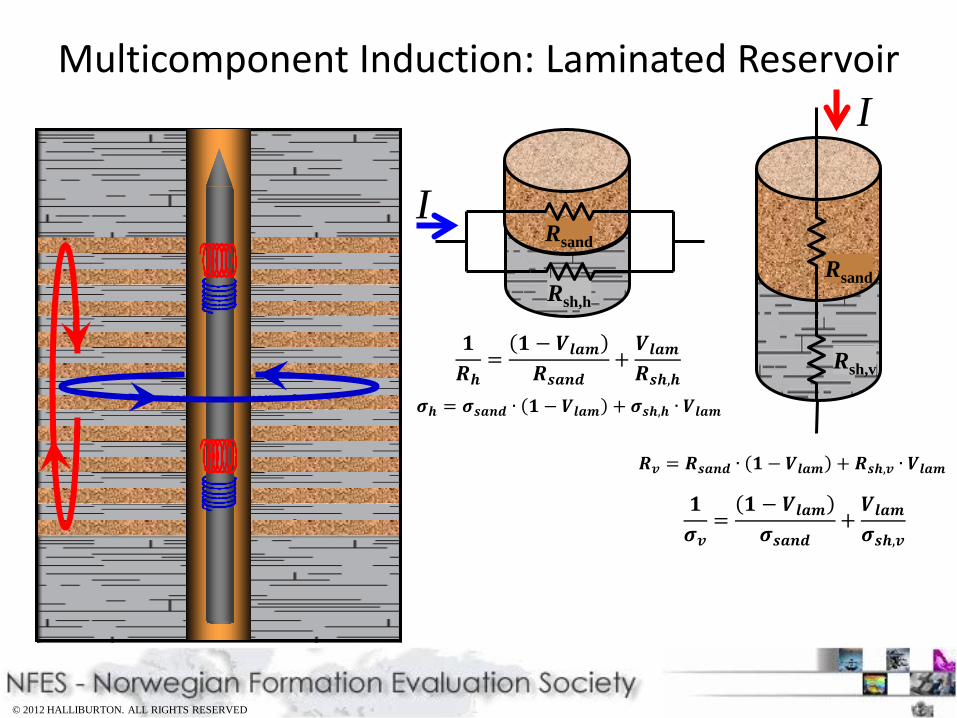
Multicomponent Induction: Laminated Reservoir
Rsand
Rsh,h
𝟏𝑹𝒉
=𝟏 − 𝑽𝒍𝒍𝒍𝑹𝒔𝒍𝒔𝒔
+𝑽𝒍𝒍𝒍𝑹𝒔𝒉,𝒉
𝝈𝒉 = 𝝈𝒔𝒍𝒔𝒔 ∙ 𝟏 − 𝑽𝒍𝒍𝒍 + 𝝈𝒔𝒉,𝒉 ∙ 𝑽𝒍𝒍𝒍
Rsand
Rsh,v
I
I
𝑹𝒗 = 𝑹𝒔𝒍𝒔𝒔 ∙ 𝟏 − 𝑽𝒍𝒍𝒍 + 𝑹𝒔𝒉,𝒗 ∙ 𝑽𝒍𝒍𝒍
𝟏𝝈𝒗
=𝟏 − 𝑽𝒍𝒍𝒍𝝈𝒔𝒍𝒔𝒔
+𝑽𝒍𝒍𝒍𝝈𝒔𝒉,𝒗

© 2012 HALLIBURTON. ALL RIGHTS RESERVED © 2012 HALLIBURTON. ALL RIGHTS RESERVED
0.1 Ω⋅m 1 Ω⋅m 10 Ω⋅m 100 Ω⋅m
𝑅𝑠𝑠,𝑠 = 𝑅𝑠𝑠,𝑣 = 1 Ω ∙ 𝑚;𝑉𝑙𝑙𝑙 = 50% 𝑅𝑠𝑙𝑖𝑖 = 10 Ω ∙ 𝑚
Rh = 1.82 Ω⋅m σh = 550 mS/m
Rv = 5.5 Ω⋅m σv = 181.8 mS/m
Multicomponent Induction: Laminated Reservoir

© 2012 HALLIBURTON. ALL RIGHTS RESERVED © 2012 HALLIBURTON. ALL RIGHTS RESERVED
Tensor Model: from Rv & Rh Rsand & Vlam
Rh
Rv • Vertical Response
• Horizontal response
• Two equations – Tool response: Rv, Rh
– Four unknowns: Rsand, Vlam, Rsh,v, Rsh,h
– Estimate from bounding shale: Rsh,v, Rsh,h
– Solution: Rsand, Vlam
𝑅𝑣 = 𝑅𝑠𝑙𝑖𝑖 ∙ 1 − 𝑉𝑙𝑙𝑙 + 𝑅𝑠𝑠,𝑣 ∙ 𝑉𝑙𝑙𝑙
1𝑅𝑠
=1 − 𝑉𝑙𝑙𝑙𝑅𝑠𝑙𝑖𝑖
+𝑉𝑙𝑙𝑙𝑅𝑠𝑠,𝑠

© 2012 HALLIBURTON. ALL RIGHTS RESERVED © 2012 HALLIBURTON. ALL RIGHTS RESERVED
Graphical Solution of Tensor Model In this plot Rh plots along x-axis and Rv along y-axis. The analyst must input the shale horizontal resistivity Rshh and the shale vertical resistivity Rshv. Mollison’s tensor equation is solved with lines of constant Rsand contoured in red. Lines of constant volume laminated shale are contoured in blue. Note zone of highest gamma ray also has greatest value of Rsand
Horizontal Resistivity
Vert
ical
Res
istiv
ity
Rshv = 11.0 Rshh = 1.3

© 2012 HALLIBURTON. ALL RIGHTS RESERVED © 2012 HALLIBURTON. ALL RIGHTS RESERVED
Thomas-Steiber Shale Distribution Model
Shale Volume, Vsh
Tota
l Por
osity
, φt 10%
20%
30%
φsh
φt,sd
φsd,max
Vlam Vdisp Vsh = Vlam + Vdisp

© 2012 HALLIBURTON. ALL RIGHTS RESERVED © 2012 HALLIBURTON. ALL RIGHTS RESERVED
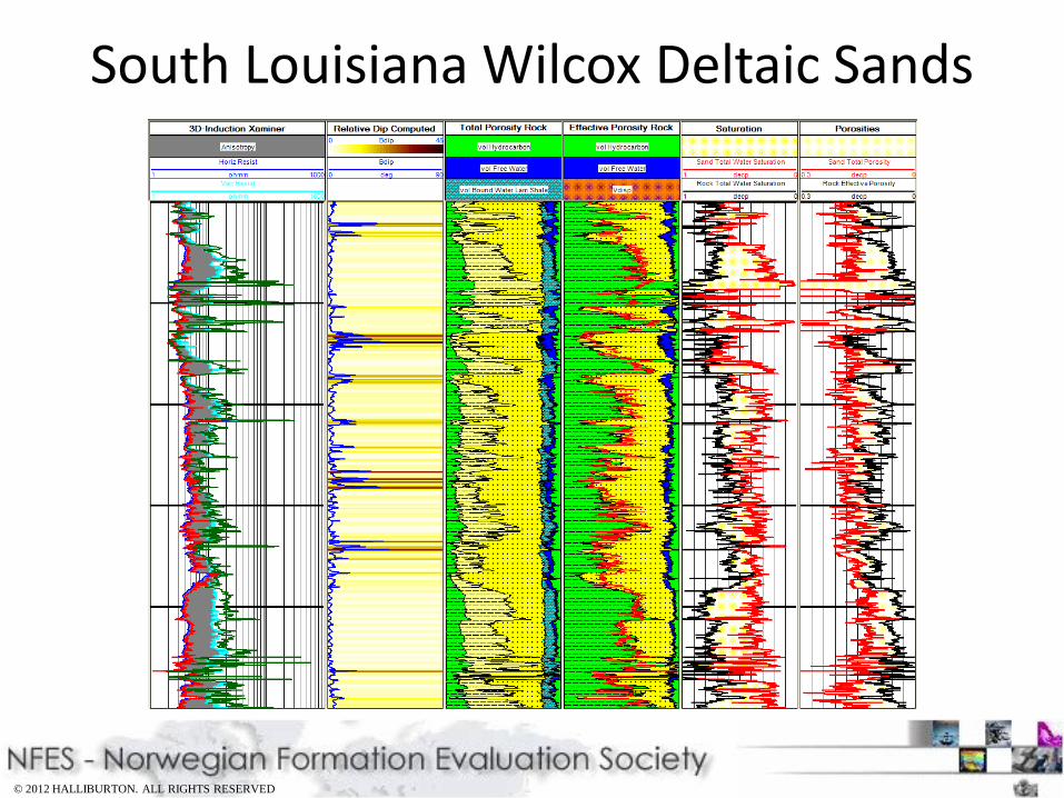
South Louisiana Wilcox Deltaic Sands

© 2012 HALLIBURTON. ALL RIGHTS RESERVED © 2012 HALLIBURTON. ALL RIGHTS RESERVED
South Louisiana Wilcox Deltaic Sands

© 2012 HALLIBURTON. ALL RIGHTS RESERVED © 2012 HALLIBURTON. ALL RIGHTS RESERVED
South Louisiana Wilcox Deltaic Sands
© 2012 HALLIBURTON. ALL RIGHTS RESERVED © 2012 HALLIBURTON. ALL RIGHTS RESERVED
South Louisiana Wilcox Deltaic Sands

© 2012 HALLIBURTON. ALL RIGHTS RESERVED © 2012 HALLIBURTON. ALL RIGHTS RESERVED
Different Resistivity Tool Types and Sensitivity to Anisotropy and Intrinsic Dip

© 2012 HALLIBURTON. ALL RIGHTS RESERVED
What does Multi-Component Induction Provide?
• Resistivity Information – Array Induction log data
• Same spacings, frequencies, processing and answers
– Rh , Rv (Resistive anisotropy ) • 3 Depths of Investigation • Radial 1D inversion • Shoulder bed correction (Vertical 1D
inversion)
• Dipmeter Information – Dip, Azimuth
• 3 Depths of Investigation • Radial 1D inversion • Shoulder Bed correction (Vertical 1D
inversion)
© 2012 HALLIBURTON. ALL RIGHTS RESERVED © 2012 HALLIBURTON. ALL RIGHTS RESERVED
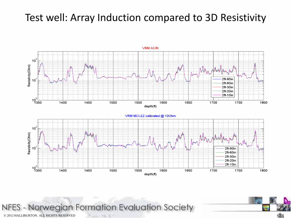
Test well: Array Induction compared to 3D Resistivity

© 2012 HALLIBURTON. ALL RIGHTS RESERVED © 2012 HALLIBURTON. ALL RIGHTS RESERVED
Test well: Array Induction compared to 3D Resistivity

© 2012 HALLIBURTON. ALL RIGHTS RESERVED © 2012 HALLIBURTON. ALL RIGHTS RESERVED
Xaminer™ MCI – Multi Component Array Induction
3D Tx
17″ 3D Rx
29″ 3D Rx
50″ 3D Rx
80″ 3D Rx
6″ & 10″ Z Rx
17.3’
No need for separate Array Induction (ACRt) - Tool provides standard ACRt outputs - Transmitter – Receiver spacing same as ACRt
Tool operates at 3 frequencies (same as ACRt) - Currently Rv, Rh only given at one frequency
1 Collocated Transmitter Triad 4 Collocated Receiver Triads with bucking coils 2 short Z Receivers Currently OBM only Rv, Rh, dip & azimuth provided at wellsite Rsand, Vlam, φsand available from post-processing