Much of the debate in macroeconomics turns on the stickiness
61
Transcript of Much of the debate in macroeconomics turns on the stickiness
1Generally, the relevant theoretical literature adopts amenu cost approach. Caplin and Spulber (1987) show that whenfirms adopt an Ss type policy in price adjustment (whichSheshinski and Weiss had shown to be optimal), and inflationaryshocks are all positive, that money is neutral. Neutrality failswhen monetary shocks can be both positive and negative, as inCaplin and Leahy (1991).
1
Much of the debate in macroeconomics turns on the stickiness
of nominal prices, to which one part of the literature ascribes
monetary non-neutrality and the propagation of demand-side business
fluctuations. Although whether micro level stickiness must lead to
substantial nominal rigidity at the aggregate level remains an open
question, certainly a prerequisite of the `New-Keynesian' approach
is that such rigidity exists at the micro level.1
I document a high degree of nominal rigidity in apartment
rents. Over the period of 1974-1981, twenty nine percent of the
apartments in my sample from the Annual Housing Survey (AHS)
National panel had no change in nominal rent from one year to the
next. About half of that fraction can be attributed to grid
pricing; the rest I interpret as downward rigidity.
The incidence varies with observable determinants in clear,
and intuitive, patterns. Nominal rigidity is higher in years and
in cities that have a low median nominal growth rate. Across
years the incidence is nearly perfectly ranked with the median
growth rate. Units that turn over have a lower, though still
substantial, incidence than those units in which the tenant stays
an additional year; however, most, and perhaps nearly all, of the
2
incidence for turnover units can be ascribed to grid pricing. The
incidence of nominal rigidity is also higher for units located in
smaller buildings.
Others have shown evidence of nominal price rigidity before,
although only for goods that represent a tiny share of consumer
expenditure. Thus Cechetti (1986) showed that even in the high
inflation decade of the 1970s, the newsstand price of magazines
remained unchanged for three and a quarter years, on average.
Kashyap (1995) followed the prices of several items, such as
chamois shirts, and fishing rods in the L. L. Bean, Orvis and
R.E.I. semiannual catalogues, and found that nominal prices
typically lasted for more than a year. Lach and Tsiddon, working
with Israeli data on 26 products - principally wine, fish and meat
-, showed that from 1978 through mid 1979, when the average monthly
inflation rate was 4 percent, the average duration of a nominal
price quotation was nonetheless 2.5-3 months. Evidence of a
different sort is provided by Levy, Bergen, Dutta and Venable
(1997) who in a recent article report for a small sample of
supermarket chains that only 70-80 percent of prices are changed in
response to wholesale price changes.
For Ball and Mankiw (1994), that the individual goods examined
are small budget items is to be expected. "For this theory, the
most important prices are for those goods bought with money, since
the price of goods bought with credit do not directly affect the
3
demand for money. Goods bought with money tend to be small retail
items, such as newspapers and haircuts." (p. 131)
One suspects, nonetheless, that the authors would be glad to
find nominal rigidity in a good that is not a "small retail item".
Indeed, housing is perhaps the one large consumer item that is not
paid with credit. For the renters of the units in my sample,
housing expenditures constitutes 20 to 30 percent of their yearly
income. Aside from the importance of this sector to the economy,
it is especially interesting to find nominal rigidity in a good
whose asset prices are known to be quite volatile.
The manner of price determination in the rental housing market
also distinguishes this good from those examined in prior research.
Unlike the market for magazines or L. L. Bean chamois shirts, where
a single seller of a homogenous good sets a price common to many
consumers, who may purchase at will, the market for rental housing
consists of heterogenous goods for which negotiation typically
attends each transaction. Few apartments are rented in the
anonymous manner of "small retail goods". Price may be tailored by
the landlord to the particular tenant, or it may be determined in
bargaining between the two. Even when a landlord follows a fixed
rent policy, the opportunity to deviate from that policy is
costlessly available, for a new contract must be produced for each
new tenant and at each lease renewal regardless of price. To use
the metaphor of "menu costs", a new menu necessarily attends every
transaction. Given this, the observed nominal rigidity must be the
2Kashyap notes that a price change requires that therelevant catalogue page be recomposed, with the attendant costs. Levy et al is quite explicitly about menu costs, which theymeasure directly. The exception is Cechetti - every magazineissue has a new cover and so could have a new price costlessly! Cechetti ascribes the nominal rigidity to coordination problemsin collusion of the sort that Sweezy’s (1939) kinked demand curveis meant to capture.
4
result of some phenomenon other than menu costs, which is the
leading explanation for nominal rigidity in the earlier studies.2
Indeed, the distribution of nominal rent changes suggests a
form of nominal rigidity more like that of downward price rigidity
than what would be produced by menu costs. Although small price
increases and decreases are relatively rare, as a menu cost
argument would predict (for a single product firm), it is the
scarcity of large negative changes that it is most striking.
Because the rarity of small absolute changes can also be explained
by grid pricing, and, as argued above, the nature of transactions
make the menu cost argument untenable, I reject the menu cost
explanation.
Of course, to speak of a certain type of price changes as
"missing" one must have a notion of what the growth of rents would
look like in the absence of nominal rigidity. In very high
inflationary periods, as in Israel during the period examined by
Lach and Tsiddon, or the Argentina of Tomassi, any change in the
real frictionless real price would typically be swamped by the
effects of inflation. The primary goal of a price setter in these
circumstances is to keep up with inflation, and so the natural

5
benchmark to which to compare nominal price changes is the
inflation rate itself. In our case, inflation was moderately high
while real rent was declining. Over the 1974-1981 period, the
consumer price index rose 84 percent while the median nominal rent
increased by 44.5 percent - or 9.2% and 5.4% annually. Thus some
benchmark other than simply the inflation rate is needed.
In constructing the counterfactual rent growth distribution,
I assume that the observed distribution is the outcome of censoring
of an underlying unobserved distribution in which some negative and
some small positive proportional increases in rent are replaced by
a zero increase in the observed data. Following Card and Hyslop’s
(1996) work on wage rigidity, I assume, additionally, that (a)
there is no censoring above the median, and (b) the underlying
distribution is symmetric. Together, this allows me to construct
the counterfactual distribution from that part of the observed
distribution above the median.
In the following section, I document how nominal rigidity
depends upon the median growth rate in nominal rent, turnover
status and building size. In section 2, I show that these results
reflect nominal rigidity across different contracts and do not
result from within lease interviewing. Section 3 discusses grid
pricing, which, in this market, is the tendency to set prices that
are multiples of certain dollar amounts. Sections 4 and 5 attempt
in various ways to determine the contribution of grid pricing to
nominal rigidity. Section 4 constructs a counterfactual
3The 1973 survey cannot be matched to the later ones. Since1981 the survey has been conducted biannually, so that AHS nowstands for the American Housing Survey. A new sample, based onthe 1980 Census, was drawn in 1985, and a 1990 Census basedsample drawn in 1995.
4SMSAs with rent control are identified primarily byNational Multihousing Council (1981 and 1982), as well as Baar(1983), Downs(1988), Gilderbloom and Applebaum (1988),Gilderbloom and Friends (1981), Capek and Gilderbloom (1992),Block and Olsen (1981), Niebanck (1985), Rydell et al (1981), and
6
distribution function which is used, first, to provide an upper
bound for, and then to explicitly calculate, the contribution of
grid pricing. In Section 5 I estimate a probit regression, thus
providing a multivariate analysis of nominal rigidity. The
regressors include a set of dummy variables for the grid point of
the previous year’s rent. Section 6 considers whether adjustments
along other margins substitute for nominal price adjustments.
Section 7 concludes.
I The Incidence Level, Turnover and Building Size
IA. Some Basic Facts
The Annual Housing Survey, National Sample (1974-1981) is a
panel of housing units, based on the 1970 Census.3 It is an
unbalanced sample, principally because samples of newly constructed
units are added each year, other units are demolished, and a few
interviews are not completed. I restrict the sample to units in
SMSAs (Standard Metropolitan Statistical Areas) with no rent
control restrictions over the 1974-1981 period.4 (The AHS gives no
The Report to Congress on Rent Control (1991).
7
location information below the state level for units outside
SMSAs.) Those cities are listed in Table 1. Of the three largest
American cities, New York City is absent as it has had rent control
of some sort or another over the post-war years, and Los Angeles is
absent since rent control was imposed in 1979, leaving Chicago the
largest city represented. Only units for which rent is paid
monthly and is recorded (rent above $1999 per month is top coded,
and I drop such units), and which are neither in public housing nor
are occupied by tenants whose rent is partly subsidized by the
government are included; these conditions are required to hold for
the year and the previous year. There are 11,418 observations,
each constituting a housing unit and two adjacent years of
completed interviews.
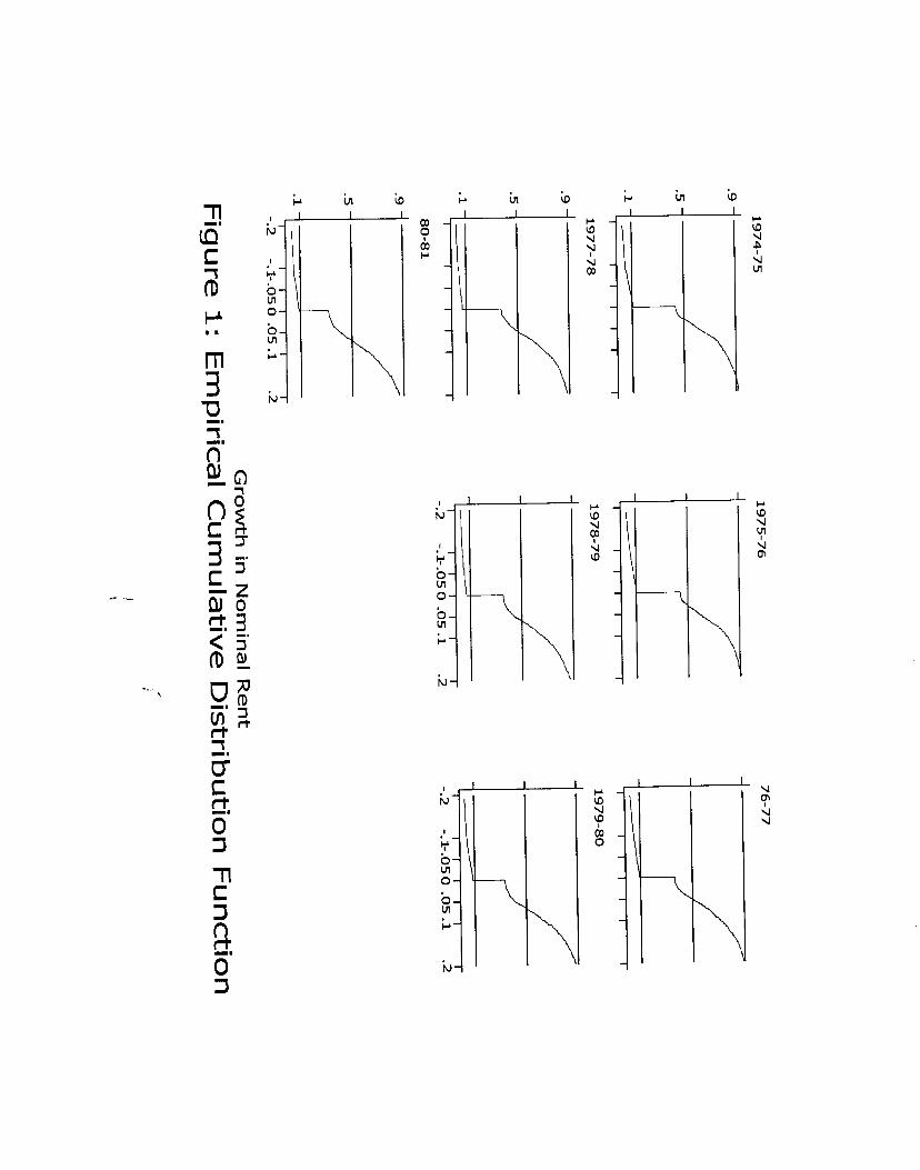
I measure a unit's nominal growth rate by dr / lnRt - lnRt-1 ,
where Rt is the nominal rent in year t. It is obtained from the
answer to the question "What is the monthly rent?" in the year t
interview. Figure 1 displays the empirical cumulative distribution
function of dr, by year. Almost all of the dispersion reflects
differences in growth rates within the SMSAS. In 1981, for
example, the overall variance of dr was .08, while the variance of
the mean dr across SMSAs was a mere .007.
The fraction of units with no nominal rent change is measured
by the length of the vertical line at zero. Clearly, there is a

8
large degree of nominal rigidity in all years. There is no
evidence of real rigidity, that is, a growth rate equal to the
inflation rate, as zero is the only "mass point" in any of the
years.
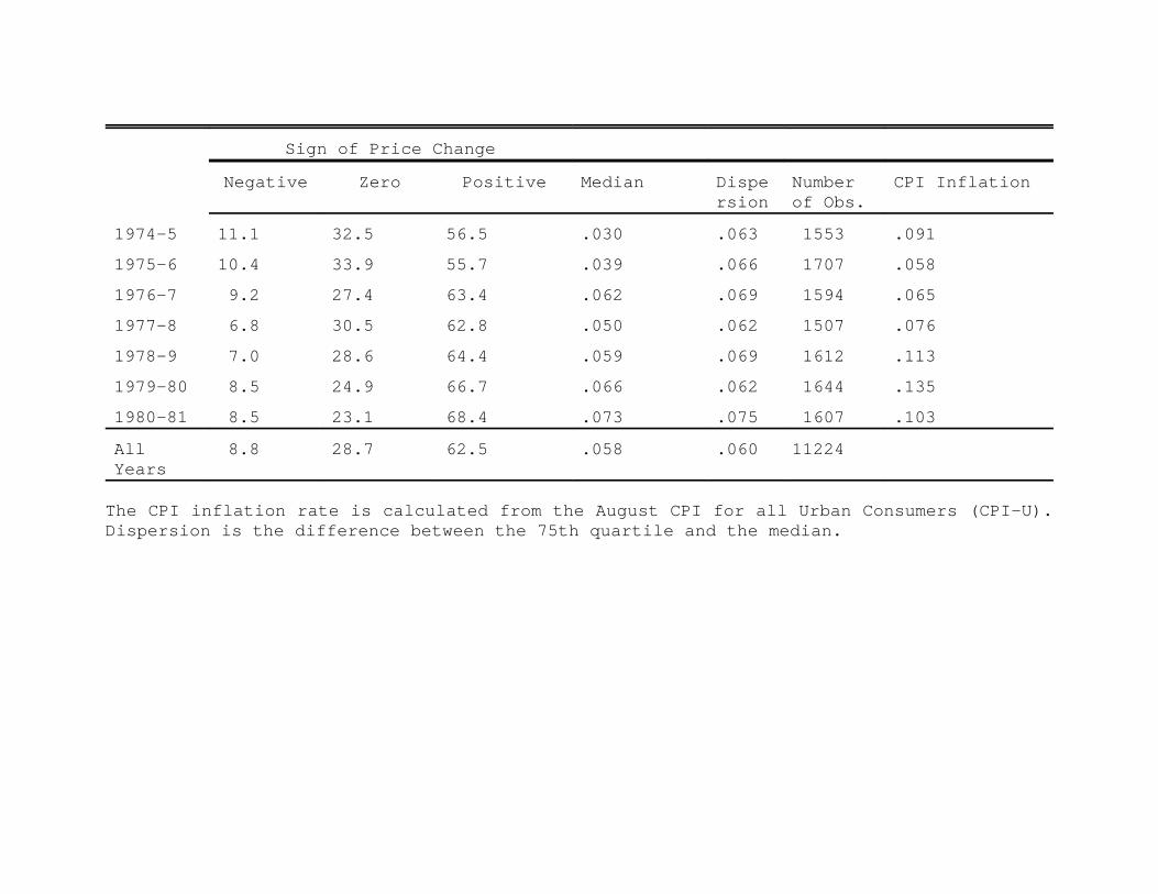
Some summary statistics of the distributions are presented in
Table 2, also by year. The incidence of nominal rigidity varies
between 23 and 34 percent, with an average of 29 percent across all
years.
Table 2 also shows that the incidence of nominal rigidity is
positively correlated with the inflation rate. This is to be
expected: a fixed nominal price is harder to sustain in an
inflationary environment. The incidence is more closely associated
with the median growth rate of nominal rent, with which it is
nearly perfectly ranked. (I choose the median as the indicator of
location, for it is natural to view zero nominal changes as
replacing what would otherwise by decreases or small increases in
the nominal rent, and the median, unlike the mean, is unaffected by
such censoring.)
The incidence of positive nominal growth is also nearly ranked
with the median. But, interestingly, the incidence of a nominal
decrease is not. This is perhaps due to the rarity of this event,
which subjects it to a greater sampling variance. But it also
suggests that much of the negative growth rates represents

5Akerlof, Dickens and Perry (1996)have similarly argued thatmost observed individual negative wage growth (within jobs) ismeasurement error.
9
measurement errors.5 Note that classical measurement error in
responses to questions about the rent level would lead to a
downward bias is measuring nominal rigidity. The table also shows
that the dispersion, measured as the difference between the median
and the 75th percentile, is relatively constant across years. I
use this measure rather than the standard deviation, because the
former is unaffected by censoring below the median.
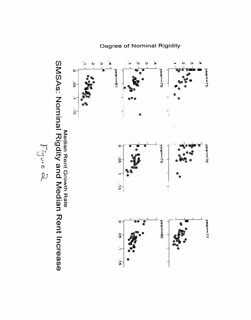
The relationship between the incidence of nominal rigidity and
the overall growth rate can be explored at the SMSA level as well.
Figure 2 plots the two against each other, by year. When the
incidence is sufficiently high, the complication of a zero median
arises, although this occurs for small SMSAS sample sizes only.
Table 3 summarizes these graphs by the regression of the nominal
incidence on the median growth rate. This can either be regarded
as merely a representation of the data, or, under the censoring
interpretation, as casual. In any case, the first column shows
that a one percent increase in the median growth rate decreases the
incidence of nominal rigidity by 1.4 percent - and predicts (out of
sample) that a median growth rate of 17 percent will exhibit no
nominal rigidity at all. Interestingly, Card and Hyslop also find
a one percent increase in inflation decreases the incidence of
nominal wage rigidity by 1.4 percent. Conditioning on SMSA or

6Tn the data for the 1979, 1980 and 1981 surveys, the Bureaucomputes a variable, HHOLD, which keeps a count of the number ofdifferent households since the 1974 survey. Increases in HHOLDcorrespond to the turnover classification described in the text96 percent of the time.
10
year, as in Columns (2) and (3), reduces the effect of median
growth rate, but the coefficient remains significant, both here and
in the remaining columns, which restrict the sample to non-zero
median rents.
IB Turnover Status
Nominal rigidity also varies with turnover status. A unit is
identified as having turned over between the two interviews if the
interviewer checked "Yes" to the statement "Household head moved
here during the last 12 months", after having posed the question:
"When did ... (head) move into this house (apartment)?", which is
answered in the year and month.6 Table 4 presents some statistics
on turnover status. The first row shows that about one-third of
all units turn over every year. The remaining rows pertain to a
subsample in which the turnover status for the previous three years
is ascertainable. They show that the turnover hazard is
decreasing: half of all units change hands after a year; of those
in which the tenant remains, one-third turn over in the year after,
with declining fractions for subsequent years.
Table 5, columns (1) through (3), displays the proportions of
units that experienced a nominal decline, nominal increase and no

11
nominal change, by tenure status and year. Overall, some 36
percent of units in which the tenant remains the same experience no
change in nominal rent, against 14 percent of units in which there
is a new tenant. The incidence of nominal rent rigidity among
continuing tenants is much greater than the fifteen percent that
Card and Hyslop report for nominal wage rigidity among their sample
of non-job changers for 1979-1992 from matched CPS data, or the
seven percent that Kahn reports for her similar, but earlier 1979-
1988 sample from the PSID. In columns (4) - (6) of the same table,
the sample is restricted to units that obtained a new tenant in the
previous year. The general pattern is always the same.
Tables 2 and 4 present two different, but related aspects of
the behavior of rental growth rates. For a complete picture, one
requires the empirical cumulative distribution function, which
Figure 3 displays, by year and by tenure status, for those units
that had turned over in the previous year. The more lightly shaded
curve represents the distribution of turnover units. There are
five noticeable aspects of this figure: (i) There is a large mass
at zero nominal change, larger for the non-turnover units but still
substantial for the turnover units. (ii) Above zero, the two
distributions differ in location only. The median growth rate for
turnover units is about four percent greater than for other units.
Notwithstanding the greater nominal rigidity of the latter units,
the mean growth rate differential is also about four percent.
(iii) Near and above zero, the distributions flatten out,

12
indicating few small positive changes. (iv) The lower tail of the
distributions are indistinguishable, except for the first two pairs
of years. (v) The non-turnover distribution is more stable over
time: variations in the location differential of the two
distributions is due to shifts in the turnover distribution.
My interpretation of the differential in median growth rates
according to tenure is that when tenants remain a second year in
the unit, there is ex-post surplus in the tenant-landlord
relationship, so that the negotiated price differs from the market
price. Furthermore, last year's nominal price represents a focal
point in bargaining. As an explanation for overall nominal
rigidity this explanation is perhaps incomplete, as it appears not
to explain nominal rigidity among turnover units. But one would
expect bargaining there, too, (once landlord and potential tenant
meet there may be some ex-post surplus because of saved search
costs) and it is not unlikely that a new tenant will know last
year's price (as when the new tenant is acquaintated with the old).
Furthermore, we will see that most, and perhaps nearly all, of the
nominal rigidity among such units can be explained by grid pricing.
Admittedly, an efficient turnover view of the housing market
undercuts the macroeconomic significance of a finding of nominal
rigidity. For under this view, using last year’s rent for this
year has only distributive, and no allocative effect.
Nevertheless, one suspects that if individuals allow nominal
concerns to determine distributional outcomes, which are as

13
important to them as allocative ones are, that nominal
considerations will affect allocative outcomes as well.
An alternative explanation is that low rents are associated
with continuing tenants because existing tenants have the first
right of refusal on the offer. Thus, according to this view, rents
determine turnover status. Discriminating between these two
explanations is the concern of another paper, but I will briefly
indicate why I think the alternative explanation is less
convincing. Consider the simplest story along these lines that one
can tell about the first renewal discount: the landlord sets a
price equal to the area wide rental growth rate, plus some random
component. We can think of this componenet as the landlord's
mistake; an equally good interpretation is that it reflects
differing discount rates or search costs among landlords. Tenants
lucky enough to have a landlord who sets a low price are more
likely to remain in the apartment.
The story falters on the dynamic effects of the observed
tenure discount. Not only is the rental growth rate 4 percent less
when the tenant continues on into a second year, it is another 5
percent less when he continues on into a third year - so that at
his second renewal date, a continuing tenant pays nine percent less
than the `market’ level. Label the random component of the rent
level set by the landlord y and the tenant’s disutility of moving
x. Assume that y is i.i.d., with distribution G, and that the
equilibrium distribution of x for (potential) first renewal
14
tenants, F1, either stochastically dominates or is dominated by the
distribution of disutility from moving for (potential) second
renewal tenants, F2. Thus either F1(x) # F2(x)for all x, or F1(x)
$ F2(x) for all x. A tenant will stay if and only if y < x. As
Table 4 showed, half of all tenants remain a second year, and two
thirds of those remain for a third year. Thus by the alternative
hypothesis, IG(x)dF1(x) - IG(x)dF2(x) = .5 - .67 < 0, so, by my
assumption, F2 stochastically dominates F1. The expected rent for
a type a tenant who stays after i years is EG[x | x # a]dFi(a), so
that the differential rent between second year tenants and third
year tenants is EG[y | y # x]d{F1(x) - F2(x)}. By the assumption
on stochastic dominance, this term must be negative. But the
opposite is true for, as I said above, third year tenants pay 5
percent less than second year tenants.
1C. Building Size
Finally, the degree of nominal rigidity also varies with the
number of "living quarters, both occupied and vacant, ..., in [the]
house (building)". Table 6 shows the incidence by building size.
We see that units in smaller buildings have a greater incidence of
nominal rigidity. It is natural to associate the number of living
quarters in the building with the number of units owned by the
landlord. A very natural explanation for this finding, then, is
that small landlords are less "professional" than large ones, so
7For example, among single detached homes, rents that arenot multiples of 5 are quoted only 5 percent of the time,compared to 26 percent of the time among units in buildings of 50or more units. The probit analysis in Section 6 shows that thedependence of nominal rigidity on building size remains, evenwhen grid pricing is controlled for.
15
that nominal rigidity is a manifestation of “irrationality”. That
grid pricing is also more prevalent in smaller buildings provides
some support for this interpretation.7
Alternatively, one might argue that large landlords simply do
not bargain with their tenants, thus eliminating the old nominal
price as a possible outcome due to its role as a focal point.
Tenants do not bargain with large landlords for the same reasons
that consumers do not bargain with large department stores,
although they might with a small retailer, or in the shuk. (These
reasons might include a strategic commitment to a price, or a
principal’s regulation of its agents, i.e., salespeople.) If this
explanation for the differential behavior of large and small
landlords is the correct one, the finding has obvious implications
for the changing sensitivity of economies to nominal shocks as they
develop and large retailing units become more prevalent.
2. Contractual vs. Non-Contractual Rigidity
To what extent does the observed nominal rigidity reflect
fixed prices within a contract? Clearly, none at all for turnover
units; the two reported rents are, by definition, from different

8Hubert's (1995) adverse selection model suggests oneexplanation for why there are so few leases longer than one year.In this model, the term of the lease is used as a screeningdevice, since good tenants will be more willing to accept shorterterm leases - or even "tenant at will" status -, at lower rents,than bad tenants.
16
contracts. For non-turnover units, whether the quoted monthly
rents originate from different contracts or not is not observable.
Unfortunately, the AHS reports neither the term of the lease - or
even if there is a lease - nor the date of the interview.
The Property Owners and Managers Survey (POMS), which was
administered to the owners or managers of a sample of units drawn
from the 1993 American Housing Survey sample, does report the term.
The POMS sample differs from the sample I use from the AHS not only
because of the difference in years, but also because, as the POMS
does not reveal the city, I cannot restrict the sample to the SMSAs
of the principle sample. However, I do drop from the POMS sample
all units not in MSAs, and units under rent control or receiving a
government subsidy.
Table 7 shows the distribution of lease terms, by building
size. Very few leases are for more than a year.8 A substantial
fraction, about fifteen percent, of units have no lease at all. Of
the remainder, about half of all leases are for a year, and half
are for less a year. Units in larger buildings are much more
likely to have a lease, and, conditional on having a lease, are

9Since units in larger buildings are more likely to have thesame lease covering both interviews, any bias resulting out ofthe timing of the interviews cannot explain why they also have alower incidence of nominal rigidity.
17
more likely to have a year-long lease.9
If one could be sure that the AHS interview dates were a year
apart then, given the distribution of lease terms, one could
conclude that the quoted rents were almost surely from different
contracts. Table 8, however, shows that the AHS is conducted in
the fall of the year over more than a one month period. It is thus
conceivable that the interviews for a given unit were conducted
less than one year apart, and so, even with a one year lease,
within the same contractual period (although it is not conclusively
so, because the Census Bureau might have surveyed the units in the
same sequence in both years, and one suspects that most of the
interviewing is concentrated at the beginning of each period). A
difference of less than one year between the two interview dates
would not alter the finding of nominal rigidity, only how much of
it can be ascribed to fixed nominal contracts.
And yet the timing of interviews does not seem to be the
reason for the nominal rigidity finding. First, note that the
reported interview periods for the 1974 and 1975 surveys overlap in
October only, whereas all the remaining pairs of years have a three
or four month overlap. If a substantial part of the nominal
rigidity were due to less than full year interview gaps, we would
expect to see a much greater degree of nominal rigidity, twice or
18
three times as much, in 1975-6 and subsequent years than in 1974-5.
Yet 1974-5 growth rates look very much like the rest.
Second, our earlier result showing that nominal rigidity was
decreasing in the SMSA median growth rate can be used to bound any
bias. There is no reason to suppose that the incidence of two
interview dates within the same lease period is at all dependant on
the median growth rate. Thus the degree of nominal rigidity at the
highest median growth rate is an upper bound to the contribution of
within lease interviewing to observed nominal rigidity. A glance
of Figure 3 shows that figure to be about 7 percent.
That upper bound is far too high, however. In columns (7)
through (9) of Table 5 the sample is restricted to units in which
the previous year's tenant originally moved in during the months of
January through July. If leases are indeed yearly, or shorter,
then interviews for these units in the Fall will capture different
contracts. Yet these columns display no reduction in nominal
rigidity. In fact, none of the results change with the restricted
sample.
The fourth piece of evidence on this point comes from the
micro level data that the Bureau of Labor Statistics collects in
constructing the CPI rent index. The BLS uses a panel of housing
units for this, returning every six months to record the apartment
rent. I have 1988-1992 data. Over those years, the degree of
nominal rigidity measured at eighteen month intervals is 37
10Unfortunately, those data do not record building size andthe tenure status variable lumps together all duration longerthan six months, making further analysis of the data along thelines of this paper impossible.
19
percent,10 which is higher than the 29% incidence that we document
here.
Finally, one also observes nominal rigidity at two year
intervals in the AHS. Ten percent of non-turnover units have the
same nominal rent in year t as in year t-2. This is more than the
seven percent one expect were nominal rigidity in one year
independent of nominal rigidity in the next. Since only 3 percent
of leases are for more than a year, most of these occurrences must
reflect rigidity across different contracts.
Taken together, all these arguments suggest very strongly
that interview gaps of less than a year are not a serious concern,
and that one may safely assume that the reported rents originate
from different leases.
3. Grid Pricing
It is sometimes asserted that observed nominal rigidity is the
outcome of the restriction to pricing on a grid: that if prices
are rounded to the nearest multiple of ten, for example, then small
underlying shocks that would otherwise lead to a change in prices
of four dollars, say, will result in no nominal change. Since what
consequences this would have for monetary neutrality appears to be
an open question, it is important to determine the extent to which
11Unfortunately, I have been unable to find any publisheddiscussion of this issue. It seems to be a matter of oral debateonly.
12Let p be the vector of data in column (a), and define the matrix A = { 1 1/2 1/4 1/12 1/20 1/100
0 1/2 1/4 1/12 1/20 1/1000 0 2/4 2/12 2/20 2/1000 0 0 8/12 8/20 8/1000 0 0 0 8/20 8/1000 0 0 0 0 80/100 }
Then column (c) is the solution to p=Ab. To understand A,consider row 4 of A, which distributes prices on the $10 gridamong the three rounding rules that could yield such an observedmodulus of $10. These are the rule of rounding to the nearest $1(of which the $10 grid provides 8 of its 100 points), a rule that
20
grid pricing is responsible for the incidence of nominal rigidity.11
Grid pricing is clearly present. Columns (a) and (b) of Table
9 shows the distribution of the modulus terms in reported rents in
1975 and 1981, respectively. For example, in 1975, 7.0 percent of
units had rents that were multiples of $100, and 8.4 percent had
rents that were multiples of $50, but not $100. I have ordered the
grid points in what seems a natural hierarchy; for example, where
there is a tendency to price at $10 intervals, there is also a
tendency to price at $25 intervals, but not necessarily vice versa.
Predictably, there is a shift in the distribution over time as
nominal prices and rents increase. Whereas in 1975, 12.8 percent
were not multiples of $5, in 1981 only 8.2 percent were.
Columns (a) and (b) overstate the extent of grid pricing. For
example, some fraction of units priced at $10 intervals reflect a
tendency to price at $5 intervals, not $10. Columns (c) and (d)
adjust for that .12 We see that almost 65 percent of rents in 1975

rounds to the nearest $5 (of which the $10 grid provides 8 of its20 points) and a rule that rounds to the nearest $10 or $25 (ofwhich the $10 grid provides 8 of 12 points - under the assumptionthat $25 is ranked above $10 in the hierarchy).
21
were priced according to a $5 grid, and that pricing on a grid
coarser than $25 was quite rare.
Grid pricing is associated with nominal rigidity. Table 10
shows the incidence of nominal rigidity by grid point. The
incidence is increasing in the hierarchy: only 12 percent of units
on a $1 grid point $1 in 1974 had zero nominal growth over 1975-4,
compared to 39 percent of units on a $100 grid point. This
difference is, of course, understated, given the comment in the
above paragraph.
Could grid pricing explain all of the price rigidity in this
market? The answer must be no. Grid pricing is relevant only to
small desired changes, and it is equally effective in turning both
desired increases and decreases into zero nominal changes. The
comparison between the empirical and the counterfactual
distribution in the next section will make that argument clearer.
4. Counterfactual Rent Growth Distributions
In this section, I construct counterfactual rent growth
distributions in order both to examine how rents would look without
nominal rigidity, and to ascertain how much of the rigidity is due
13Khan (1998) assumes, in contrast, that uncensoreddistributions from different years differ only in a locationparameter. This allows her to uses the location-correcteddistribution of a year with small nominal rigidity as acounterfactual. The method is less useful here, since nominalrigidity is high in all years and as I need a “continuous”counterfactual distribution to predict the extent of gridpricing.
22
to grid pricing.
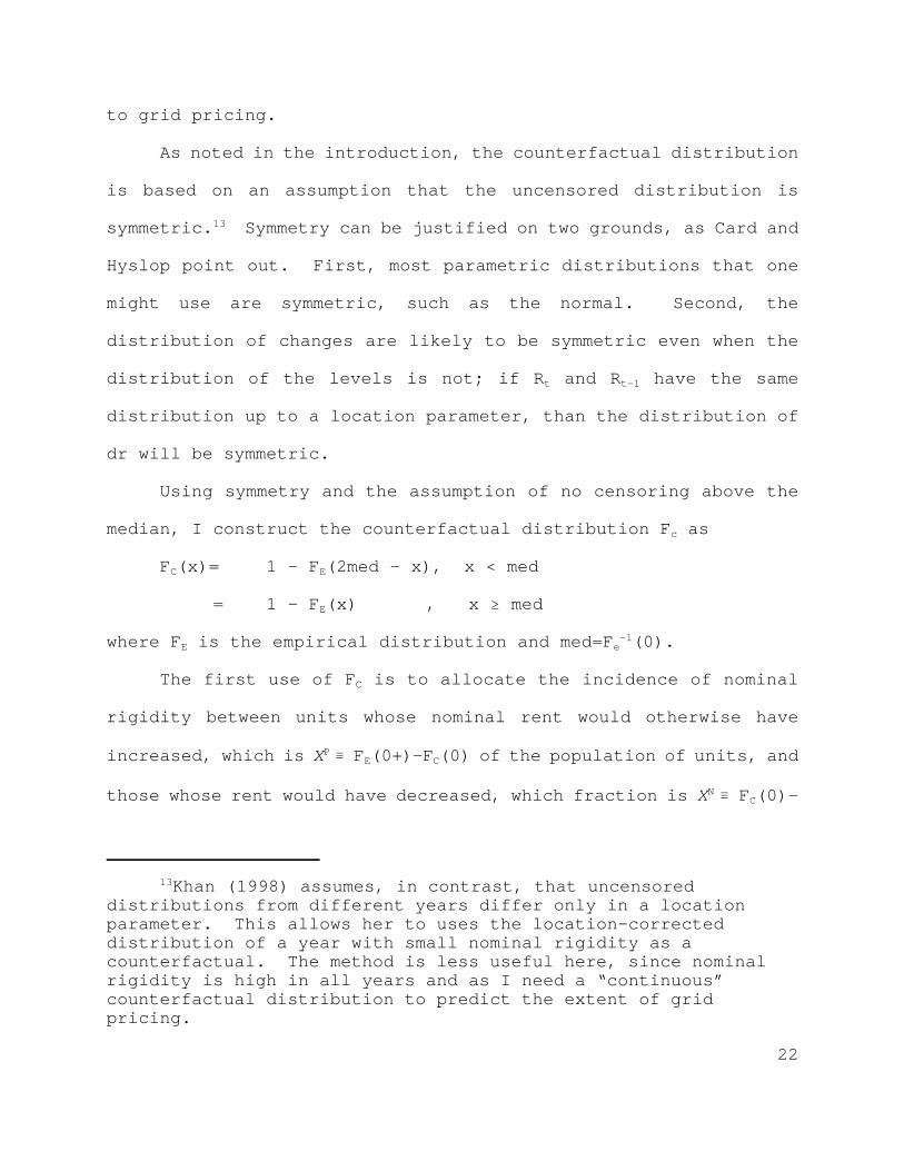
As noted in the introduction, the counterfactual distribution
is based on an assumption that the uncensored distribution is
symmetric.13 Symmetry can be justified on two grounds, as Card and
Hyslop point out. First, most parametric distributions that one
might use are symmetric, such as the normal. Second, the
distribution of changes are likely to be symmetric even when the
distribution of the levels is not; if Rt and Rt-1 have the same
distribution up to a location parameter, than the distribution of
dr will be symmetric.
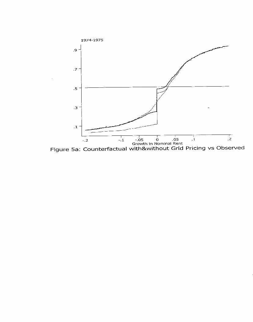
Using symmetry and the assumption of no censoring above the
median, I construct the counterfactual distribution Fc as
FC(x)= 1 - FE(2med - x), x < med
= 1 - FE(x) , x $ med
where FE is the empirical distribution and med=Fe-1(0).
The first use of FC is to allocate the incidence of nominal
rigidity between units whose nominal rent would otherwise have
increased, which is XP / FE(0+)-FC(0) of the population of units, and
those whose rent would have decreased, which fraction is XN / FC(0)-
23
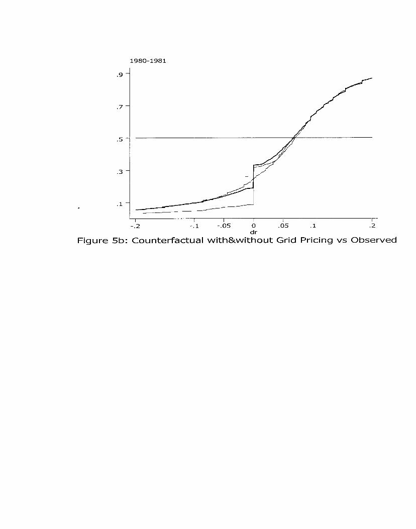
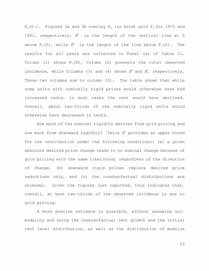
FE(0-). Figures 3a and 3b overlay Fe (in bold) with Fc for 1975 and
1981, respectively. XP is the length of the vertical line at 0
above FC(0), while XN is the length of the line below FC(0). The
results for all years are collected in Panel (a) of Table 11.
Column (1) shows FC(0), Column (2) presents the total observed
incidence, while Columns (3) and (4) shows XP and XN, respectively.
These two columns sum to column (2). The table shows that while
some units with nominally rigid prices would otherwise have had
increased rents, in most cases the rent would have declined.
Overall, about two-thirds of the nominally rigid units would
otherwise have decreased in rents.
How much of the nominal rigidity derives from grid pricing and
how much from downward rigidity? Twice XP provides an upper bound
for the contribution under the following conditions: (a) a given
absolute desired price change leads to no nominal change because of
grid pricing with the same likelihood, regardless of the direction
of change, (b) downward rigid prices replace desired price
reductions only, and (c) the counterfactual distributions are
unimodal. Given the figures just reported, this indicates that,
overall, at most two-thirds of the observed incidence is due to
grid pricing.
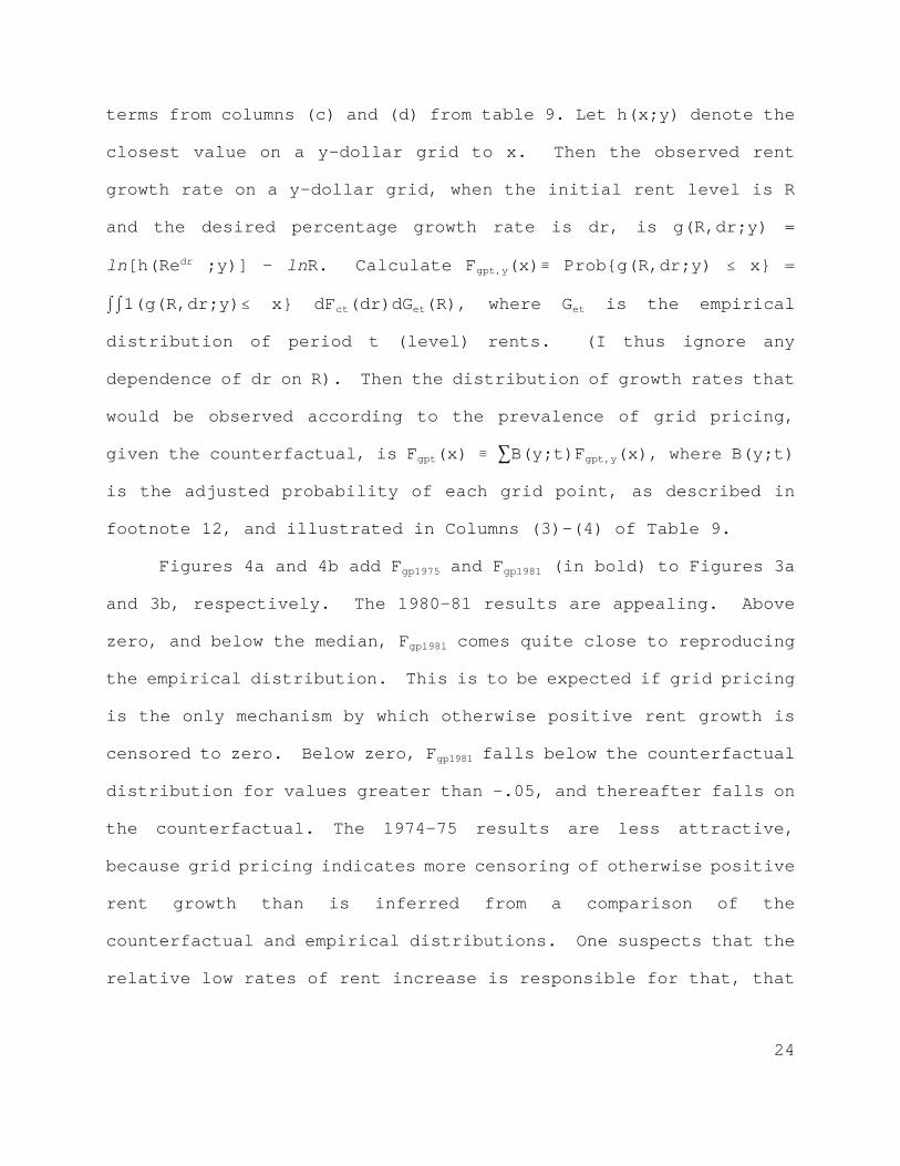
A more precise estimate is possible, without assuming uni-
modality and using the counterfactual rent growth and the initial
rent level distribution, as well as the distribution of modulus
24
terms from columns (c) and (d) from table 9. Let h(x;y) denote the
closest value on a y-dollar grid to x. Then the observed rent
growth rate on a y-dollar grid, when the initial rent level is R
and the desired percentage growth rate is dr, is g(R,dr;y) =
ln[h(Redr ;y)] - lnR. Calculate Fgpt,y(x)/ Prob{g(R,dr;y) # x} =
II1(g(R,dr;y)# x} dFct(dr)dGet(R), where Get is the empirical
distribution of period t (level) rents. (I thus ignore any
dependence of dr on R). Then the distribution of growth rates that
would be observed according to the prevalence of grid pricing,
given the counterfactual, is Fgpt(x) / 3B(y;t)Fgpt,y(x), where B(y;t)
is the adjusted probability of each grid point, as described in
footnote 12, and illustrated in Columns (3)-(4) of Table 9.
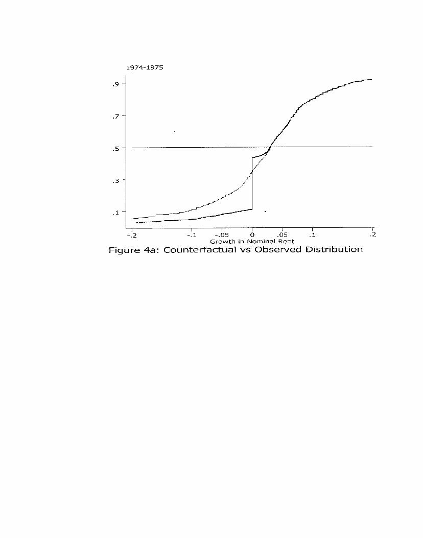
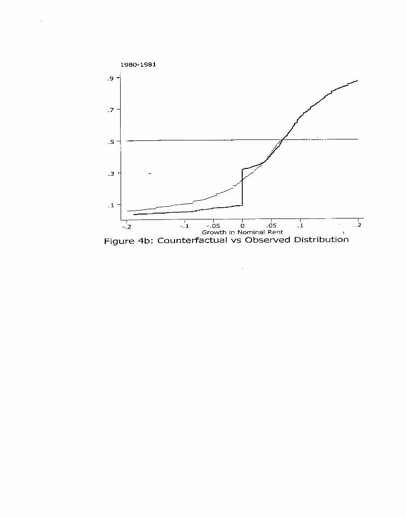
Figures 4a and 4b add Fgp1975 and Fgp1981 (in bold) to Figures 3a
and 3b, respectively. The 1980-81 results are appealing. Above
zero, and below the median, Fgp1981 comes quite close to reproducing
the empirical distribution. This is to be expected if grid pricing
is the only mechanism by which otherwise positive rent growth is
censored to zero. Below zero, Fgp1981 falls below the counterfactual
distribution for values greater than -.05, and thereafter falls on
the counterfactual. The 1974-75 results are less attractive,
because grid pricing indicates more censoring of otherwise positive
rent growth than is inferred from a comparison of the
counterfactual and empirical distributions. One suspects that the
relative low rates of rent increase is responsible for that, that

25
is, censoring occurs above the median.
The predicted nominal rigidity from grid pricing alone is then
Fgpt(0+)-Fgpt(0-), which is shown in Column (5) of Table 11. Column
(6) subtracts Column (5) from Column (2); this is the incidence of
nominal rigidity, net of the predicted amount from grid pricing.
We see that, overall, of the 29 percent incidence, only 11 percent
can not be explained by grid pricing. This is somewhat higher than
the lower bound of nine percent obtained from subtracting twice XP
from Column (2).
If one conditions on turnover status, an interesting pattern
emerges. Panels (b) and (c) of Table 11 restrict the sample to
units that turned over in the previous period. Panel (b)’s sample
is further restricted to units which did not turn over in the
current period, while panel (c) includes the units that did turn
over. Net of predicted rigidity due to grid pricing, the incidence
of nominal rigidity is 21 percent of the continuing units, while
only 3 percent among the turn over units. In other words, grid
pricing can explain somewhat less than half of the nominal rigidity
observed among turnover, while it can explain almost all of it
among continuing units.
5. Multivariate Analysis
The single variate analysis thus far begs the question of
whether any of these relationships are spurious. Because the
26
sample size is not large enough to form cells of an adequate number
of observations in all cases, I consider the ad hoc expedient of a
probit analysis of nominal rigidity.
Estimates from the probit regressions are presented in Table
12. The dependent variable takes the value 1 if the nominal growth
in rent is zero. All the regressors are dummy variables, with the
dummy variables for a $1 grid point, a 50 or more unit building,
1980-1 and a turnover unit serving as the omitted dummies,
depending on the set of dummies included in each regression. Each
of these values correspond to the cell with the lowest nominal
rigidity, as indicated in the previous tables. Jointly, they
define a baseline case, whose probability of nominal rigidity is
given by the row labeled M(constant).
The first three columns use the whole sample. Column (1)
considers only the effect of the modulus t-1 rent. Column (2) adds
dummy variables for the building size. We see that both sets of
variables effect nominal rigidity. Column (3) adds year dummies.
The remaining columns restrict the sample to units that turned
over in the previous year. Columns (4)-(6) repeat the earlier
analysis for the restricted sample. Column (7) adds a dummy
variable for units that did not turn over. The constant term in
that Column indicates that (i) in 1981 (when median rents were
increasing at 7 percent), a unit (ii) in a 50 plus unit building
(iii) which turned over that year, and (iv) for which the previous
year’s price was set on a grid no coarser than one dollar, had only
27
a two percent probability of having an unchanged nominal rent.
Given that none of these variables should be correlated with within
lease interviewing, we can once more conclude that observed nominal
rigidity is not an artifact of within term interviewing, along the
lines of the second point in Section 2.
If the unit was detached, instead, the probability of nominal
rigidity would increase to 12 percent; if it did not turn over, the
probability would be six percent more than the baseline case. A
unit that was both detached and did not turn over, would have an
incidence of nominal rigidity of 28 percent. If, in addition, the
previous year’s price was set on a $100 grid, the probability would
double to 56 percent. Thus, we see that the previous findings are
not the results of spurious correlations. Each factor effects
nominal rigidity in the same way that was demonstrated earlier,
even when controlling for the others.
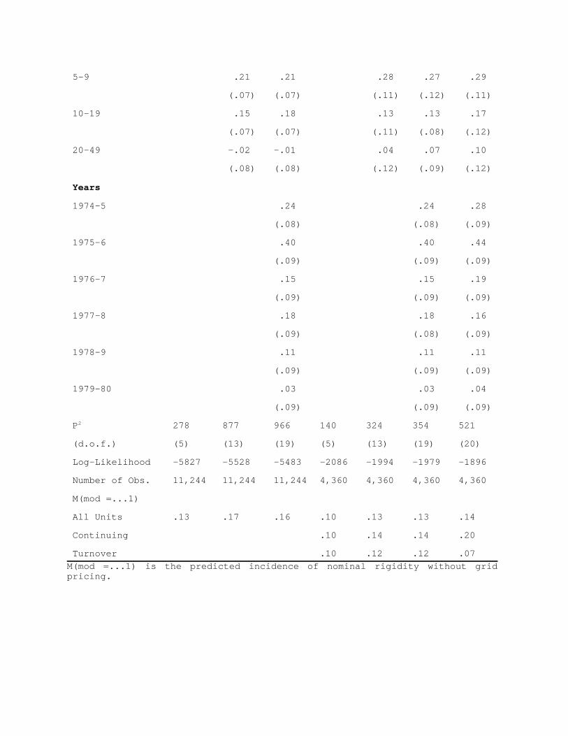
Finally, we can use the probit estimates to predict the degree
of nominal rigidity we would observe in the absence of grid
pricing. This approach has the advantage over constructing a
counterfactual distribution with grid pricing, in that it places
grid pricing and any remaining determinants of nominal rigidity on
an equal footing. In Table 11, in contrast, nominal rigidity that
would have arisen both because of grid pricing and because the unit
was in a small building, say, is allocated to grid pricing.
To get the predicted incidence of nominal rigidity, net of
grid pricing, I sum over the predicted probabilities obtained when

28
the grid point dummies in Table 12 are all set equal to zero, and
all other variables set to their actual values. The mean predicted
incidence is presented in the last rows of the table. As expected,
these are somewhat higher than the values shown in Column (6) of
Table 11. Over all years, we see that the predicted net incidence
is 16 percent in the whole sample (compared to 11 percent from
Table 11). On the sub-sample of units that turned over in the
previous period, it is 20 percent among the continuing units and,
and 7 percent among those that turned over, (compared to 19 percent
and 3 percent from Table 11).
6. Other Margins
The rent is not the only means by which the overall terms of
trade between tenant and landlord might be altered. They are also
determined by the assignment of responsibility for payment of
utilities. As an instrument for splitting the surplus between
landlord and tenant, this is a poor substitute for the rent, of
course. Not only is it coarser than a change in the rent itself
can be, but efficiency considerations will dictate their own
assignment. In an efficient contract, which party pays the heating
bill will depend on the monitoring cost, the price of the fuel and
the elasticity of the demand for heating. The rent is the natural
instrument to distribute the surplus. Nonetheless, there are two
grounds on which to investigate whether these provisions are used

14The quality-adjusted price can also be changed by alteringthe level of maintenance. Likewise, as long as the quality ofthe unit is not a perfect substitute for “other goods” (money),there will be an efficient level of maintenance. I considerchanges in the assignment of responsibility to pay utilities butnot changes in quality, because the former is an objective,whereas the latter, as reported by the tenant, will be verysubjective.
29
as well. First, were nominal rigidity in the rent accompanied by
offsetting changes to other terms of the contract between the
landlord and the tenant, its macroeconomic consequences might be
altered. Second, it would be useful to know if such inefficiencies
arise out of nominal rigidity. Where there is nominal illusion,
there may be inefficient contracts as well. Nominal illusion might
lead to inefficiency in this way.14
Table 13 (14) shows the proportion of units in which the
tenant pays the electricity (gas) bill according to whether the
nominal rent changes or not, and according to which party bore the
responsibility in the previous year. The rows titled “All Units”
show that there is little year to year change in the assignment of
responsibility for paying the fuel bills. The greater likelihood
of a transition from the landlord paying the utility bill to the
tenant than vice versa can be explained by the increase in fuel
prices during this period, as well as the fact that installing
monitoring equipment is a sunk investment.
When the tenant was previously responsible for the electricity
bill, the total real housing cost to the renter can be reduced by
more than the inflation rate when keeping the nominal rent

30
unchanged by levying the electricity bill on the landlord instead.
But the left panel of Table 13 shows that reallocation occurring in
a mere half a percent of the cases in which the nominal rent is
unchanged; furthermore, that is fewer than the proportion of cases
when the nominal rent does change, which is one and a half percent.
Likewise, when the electricity bill was previously paid by the
landlord, the total real housing cost to the renter can be reduced
by less than the inflation rate, or even increased, when keeping
the nominal rent unchanged by levying the electricity bill on the
tenant instead. That is done in only six percent of the relevant
cases; again, this is less often than when there is a nominal
change.
In this discussion, I have described Table 13 only, but the
reader can see that the assignment of responsibility to pay gas
bills follows the same basic patterns. These results clearly
indicate that changes in the assignment of responsibility to pay
the utility bills do not compensate for nominal rigidity, and, if
anything, are complementary to it.
7. Conclusion
This paper has shown that there is substantial nominal
rigidity in apartment rents, and that it varies in definite
patterns. This finding gives credence to macroeconomic models that
rely on such rigidities to explain aggregate economic fluctuations.

31
About half of the incidence can be attributed to grid pricing. It
is an open question whether the macroeconomic consequences of
nominal rigidity are dependent on grid pricing or not.
Although I have motivated this paper by the macro literature
on price stickiness, there are obvious microeconomic issues as
well. Even if grid pricing does not lead to price rigidity at the
macro level, it is still interesting at the micro level as a
manifestation of “irrationality”. Also at the micro level, the
difference between the incidence levels among new and continuing
tenants suggests that the old nominal price is a focal point in
bargaining. This implies that nominal values have distributive
consequences. They will have allocative consequences as well, when
bargaining is not efficient.

32
References
Akerlof, George, William Dickens and George Perry, "TheMacroeconomics of Low Inflation," Brookings Papers on EconomicActivity, 1996, 1 1-76.
Baar, Kenneth 1983. “Guidelines for drafting rent control laws:Lessons of a decade” Rutgers Law Review, 35(4):721-885.
Ball, Lawrence and N. Gregory Mankiw, "A Sticky-Price Manifesto",Carnegie Rochester Conference Series on Public Policy, Vol. 41(1994), 127-151.
Block, W. and E. Olsen, Rent Control: Myths and Realities, TheFraser Institute, Vancouver 1981.
Caballero, R. J. and E. Engel, “Dynamic (S-s) Economies”,Econometrica, 59 (1991), 1659-86.
Capek, Stella M. and John I. Gilderbloom. Community versusCommodity: Tenants and the American City, State University of NewYork Press, Albany 1992.
Caplin, A. and D. Spulber, "Menu Costs and the Neutrality ofMoney", Quarterly Journal of Economics, 102 (1987) 703-725.
Caplin, A. and J. Leahy, "State Dependent Pricing and the Dynamicsof Money and Output," Quarterly Journal of Economics, 106 (1991)683-708.
Card, D. and D. Hyslop, "Does Inflation "Grease the Wheels of theLabor Market?”" in Christina D. Romer and David H. Romer, ReducingInflation: Motivation and Strategy, 1996, 71-120.
Cecchetti, Stephen G. "The Frequency of Price Adjustment: A Studyof the Newsstand Prices of Magazines," Journal of Econometrics 31(1986) 255-274.
Downs, Anthony. Residential Rent Controls: An Evaluation, TheUrban Land Institute, WAshington D.C., 1988.
Gilderbloom John et al. Rent Control: A Source Book, Foundationfor National Progress, Housing Information Center, 1981.
Gilderbloom, John and Richard P. Appelbaum. Rethinking Rental
33
Housing, Temple University Press, 1988.
Hubert, F. "Contracting with Costly Tenants", Regional Science andUrban Economics, 25 (1995) 631-654.
Kahn, S. "Evidence of Nominal Wage Stickiness from Microdata,"American Economic Review, 1998.
Kashyap, "Sticky Prices: New Evidence from Retail Catalogs",Quarterly Journal of Economics, 110 (1995) 245-274.
Lach, S. and D. Tsiddon, "The Behavior of Prices and Inflation:An Empirical Analysis of Disaggregated Price Data", Journal ofPolitical Economy, April 1992 100 (2), 349-89.
Lach, S. and D. Tsiddon, "Staggering and Synchronization in Price-Setting: Evidence from Multiproduct Firms" American EconomicReview, December 1996, 86 (5), 1175-1196.
Levy, Daniel, Mark Bergern, Shantanu Dutta, and Robert Venable."The Magnitude of Menu Costs: Direct Evidence from Large U.S.Supermarket Chains", Quarterly Journal of Economics, August 1997,CX11 (3), 791-826.
Niebanck, Paul L., ed. The Rent Control Debate, The University ofNorth Carolina Pres, Chapel Hill, 1985.
National Multi Housing Council The Spread of Rent Control 1981 and1982, Washington, D.C.
Rydell, Peter C., C. Lance Barnett, Carol E. Hillestad, Michael P.Murray, Kevin Neels and Robert H. Sims, 1981. “The impact of rentcontrol on the Los Angeles Housing Market” N-1747-LA (RAND).
Shesinski, E. and Y. Weiss, "Optimum Pricing Policy UnderStochastic Inflation," Review of Economic Studies, 50 (1983), 513-529.
Sweezy, Paul. “Demand Under Conditions of Oligopoly”, Journal ofPolitical Economy 47: 568-573.
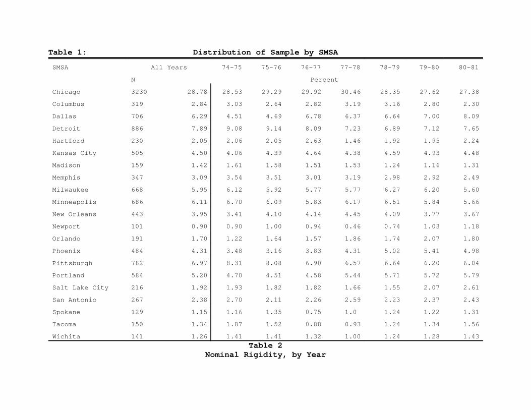
Table 1: Distribution of Sample by SMSA
SMSA All Years 74-75 75-76 76-77 77-78 78-79 79-80 80-81
N Percent
Chicago 3230 28.78 28.53 29.29 29.92 30.46 28.35 27.62 27.38
Columbus 319 2.84 3.03 2.64 2.82 3.19 3.16 2.80 2.30
Dallas 706 6.29 4.51 4.69 6.78 6.37 6.64 7.00 8.09
Detroit 886 7.89 9.08 9.14 8.09 7.23 6.89 7.12 7.65
Hartford 230 2.05 2.06 2.05 2.63 1.46 1.92 1.95 2.24
Kansas City 505 4.50 4.06 4.39 4.64 4.38 4.59 4.93 4.48
Madison 159 1.42 1.61 1.58 1.51 1.53 1.24 1.16 1.31
Memphis 347 3.09 3.54 3.51 3.01 3.19 2.98 2.92 2.49
Milwaukee 668 5.95 6.12 5.92 5.77 5.77 6.27 6.20 5.60
Minneapolis 686 6.11 6.70 6.09 5.83 6.17 6.51 5.84 5.66
New Orleans 443 3.95 3.41 4.10 4.14 4.45 4.09 3.77 3.67
Newport 101 0.90 0.90 1.00 0.94 0.46 0.74 1.03 1.18
Orlando 191 1.70 1.22 1.64 1.57 1.86 1.74 2.07 1.80
Phoenix 484 4.31 3.48 3.16 3.83 4.31 5.02 5.41 4.98
Pittsburgh 782 6.97 8.31 8.08 6.90 6.57 6.64 6.20 6.04
Portland 584 5.20 4.70 4.51 4.58 5.44 5.71 5.72 5.79
Salt Lake City 216 1.92 1.93 1.82 1.82 1.66 1.55 2.07 2.61
San Antonio 267 2.38 2.70 2.11 2.26 2.59 2.23 2.37 2.43
Spokane 129 1.15 1.16 1.35 0.75 1.0 1.24 1.22 1.31
Tacoma 150 1.34 1.87 1.52 0.88 0.93 1.24 1.34 1.56
Wichita 141 1.26 1.41 1.41 1.32 1.00 1.24 1.28 1.43
Table 2Nominal Rigidity, by Year
Sign of Price Change
Negative Zero Positive Median Dispersion
Number of Obs.
CPI Inflation
1974-5 11.1 32.5 56.5 .030 .063 1553 .091
1975-6 10.4 33.9 55.7 .039 .066 1707 .058
1976-7 9.2 27.4 63.4 .062 .069 1594 .065
1977-8 6.8 30.5 62.8 .050 .062 1507 .076
1978-9 7.0 28.6 64.4 .059 .069 1612 .113
1979-80 8.5 24.9 66.7 .066 .062 1644 .135
1980-81 8.5 23.1 68.4 .073 .075 1607 .103
AllYears
8.8 28.7 62.5 .058 .060 11224
The CPI inflation rate is calculated from the August CPI for all Urban Consumers (CPI-U).Dispersion is the difference between the 75th quartile and the median.

Table 3
Nominal Rigidity and Median Rent
Whole Sample Median Rent > 0
(1) (2) (3) (4) (5) (6)
Median Rent -1.36 -1.07 -.92 -1.0 -.84 -.67
(.10) (.10) (.11) (.11) (.11) (.11)
Constant .24 .22 .21
(.01) (.01) (.01)
P2-stat (d.o.f.)
YEAR 7.5 (6) 9.9 (6) 5.6 (6) 7.5 (6)
SMSA 2.6 (39) 2.4 (39)
R2 .46 .55 .70 .66
N 245 245 245 203 203 203
Both the mean and the median of the Median Rent in the whole sample is .05, while thestandard deviation is .03.

Table 4Turnover Status
Percent that turn over inyear t
Number of Obs.
All Units 34.9 11224
Units that last turned overin ...
t - 1 49.4 1819
t - 2 36.3 921
t - 3 29.3 673
t - 4 or earlier 15.9 2155
t - 1 or earlier 31.8 5568

Table 5 Nominal Rigidity by Turnover Status and Year
Whole Sample Unit Turned Over inPrevious Period
January - JulySubsample
(1) (2) (3) (4) (5) (6) (7) (8) (9)
Neg. Zero Pos. Neg. Zero Pos. Neg. Zero Pos.
1974-5 C 9 40 51 10 41 49 9 40 51
T 15 19 67 17 21 62 18 21 61
N 1553 579 883
1975-6 C 10 40 50 8 47 44 10 41 50
T 11 21 68 12 28 60 16 20 65
N 1707 622 837
1976-7 C 9 35 56 11 38 50 9 34 57
T 9 14 77 9 18 73 13 16 71
N 1594 605 880
1977-8 C 6 40 54 7 40 53 10 37 53
T 8 12 80 9 16 75 11 10 80
N 1507 616 833
1978-9 C 7 37 56 7 43 50 9 35 57
T 7 12 81 8 12 80 9 10 81
N 1612 612 870
1979-80 C 8 32 60 10 34 56 9 30 61
T 9 12 79 10 16 74 7 10 82
N 1644 655 1044
1980-1 C 8 30 61 7 35 58 8 33 59
T 9 10 81 10 13 77 8 10 81
N 1607 671 822
The January - July sub-sample (columns (7)-(9))is restricted to observations forwhich the previous year's tenant originally moved into the unit in the months ofJanuary through July.
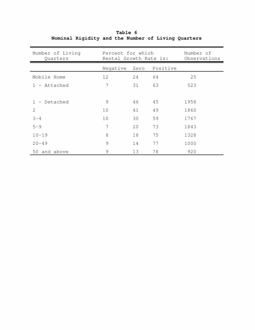
Table 6Nominal Rigidity and the Number of Living Quarters
Number of Living Quarters
Percent for which Rental Growth Rate is:
Number ofObservations
Negative Zero Positive
Mobile Home 12 24 64 25
1 - Attached 7 31 63 523
1 - Detached 9 46 45 1958
2 10 41 49 1860
3-4 10 30 59 1767
5-9 7 20 73 1843
10-19 8 18 75 1328
20-49 9 14 77 1000
50 and above 9 13 78 920
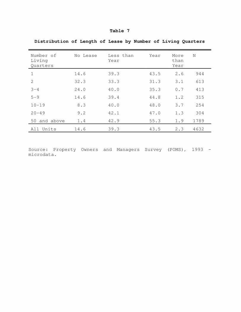
Table 7
Distribution of Length of Lease by Number of Living Quarters
Number ofLiving Quarters
No Lease Less thanYear
Year MorethanYear
N
1 14.6 39.3 43.5 2.6 944
2 32.3 33.3 31.3 3.1 613
3-4 24.0 40.0 35.3 0.7 413
5-9 14.6 39.4 44.8 1.2 315
10-19 8.3 40.0 48.0 3.7 254
20-49 9.2 42.1 47.0 1.3 304
50 and above 1.4 42.9 55.3 1.9 1789
All Units 14.6 39.3 43.5 2.3 4632
Source: Property Owners and Managers Survey (POMS), 1993 -microdata.

Table 8Interview Period of the Annual Housing Survey
Year Interview Period
1974 August-October
1975 October-December
1976 October-December
1977 October-January
1978 October-January
1979 September-December
1980 mid August-December
1981 September- December
Source: Annual Housing Survey, United States and Region Part A:General Housing Characteristics, U.S. Department of CommerceSeries H-150, various years.
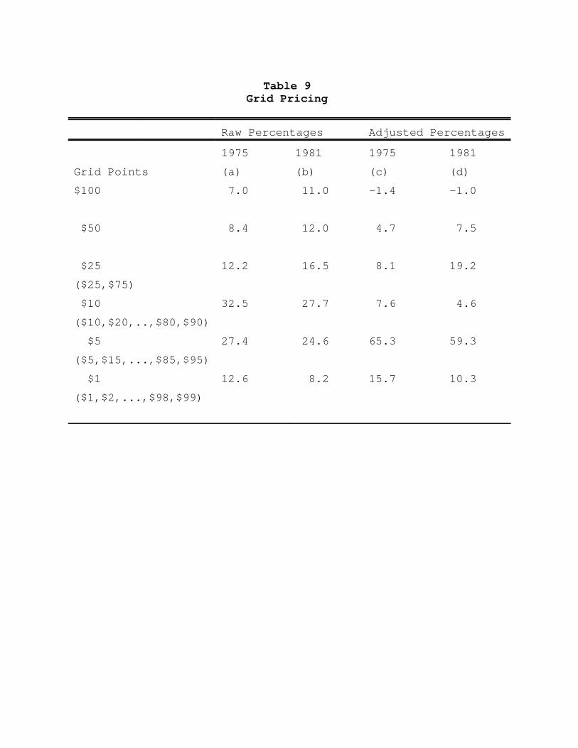
Table 9Grid Pricing
Raw Percentages Adjusted Percentages
1975 1981 1975 1981
Grid Points (a) (b) (c) (d)
$100 7.0 11.0 -1.4 -1.0
$50 8.4 12.0 4.7 7.5
$25 12.2 16.5 8.1 19.2
($25,$75)
$10 32.5 27.7 7.6 4.6
($10,$20,..,$80,$90)
$5 27.4 24.6 65.3 59.3
($5,$15,...,$85,$95)
$1 12.6 8.2 15.7 10.3
($1,$2,...,$98,$99)
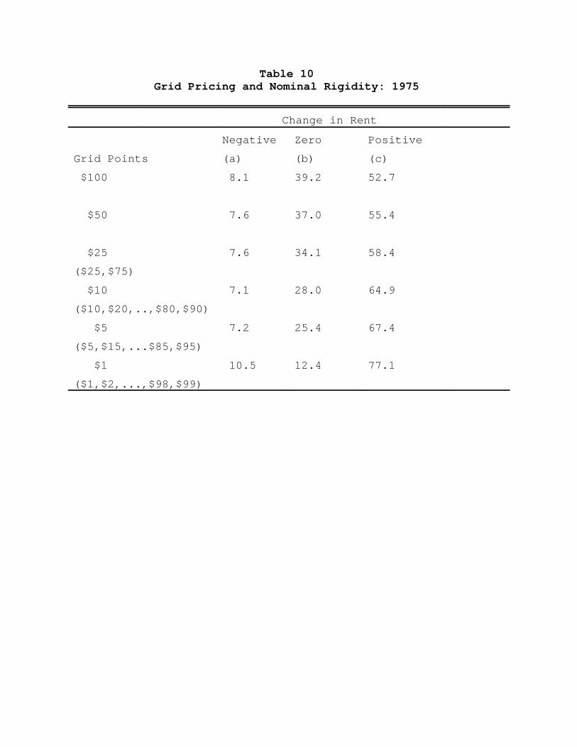
Table 10Grid Pricing and Nominal Rigidity: 1975
Change in Rent
Negative Zero Positive
Grid Points (a) (b) (c)
$100 8.1 39.2 52.7
$50 7.6 37.0 55.4
$25 7.6 34.1 58.4
($25,$75)
$10 7.1 28.0 64.9
($10,$20,..,$80,$90)
$5 7.2 25.4 67.4
($5,$15,...$85,$95)
$1 10.5 12.4 77.1
($1,$2,...,$98,$99)
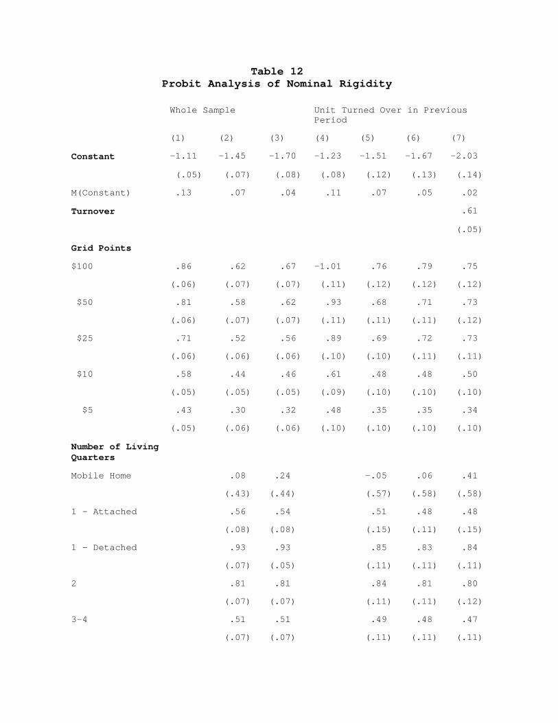
Table 12Probit Analysis of Nominal Rigidity
Whole Sample Unit Turned Over in PreviousPeriod
(1) (2) (3) (4) (5) (6) (7)
Constant -1.11 -1.45 -1.70 -1.23 -1.51 -1.67 -2.03
(.05) (.07) (.08) (.08) (.12) (.13) (.14)
M(Constant) .13 .07 .04 .11 .07 .05 .02
Turnover .61
(.05)
Grid Points
$100 .86 .62 .67 -1.01 .76 .79 .75
(.06) (.07) (.07) (.11) (.12) (.12) (.12)
$50 .81 .58 .62 .93 .68 .71 .73
(.06) (.07) (.07) (.11) (.11) (.11) (.12)
$25 .71 .52 .56 .89 .69 .72 .73
(.06) (.06) (.06) (.10) (.10) (.11) (.11)
$10 .58 .44 .46 .61 .48 .48 .50
(.05) (.05) (.05) (.09) (.10) (.10) (.10)
$5 .43 .30 .32 .48 .35 .35 .34
(.05) (.06) (.06) (.10) (.10) (.10) (.10)
Number of LivingQuarters
Mobile Home .08 .24 -.05 .06 .41
(.43) (.44) (.57) (.58) (.58)
1 - Attached .56 .54 .51 .48 .48
(.08) (.08) (.15) (.11) (.15)
1 - Detached .93 .93 .85 .83 .84
(.07) (.05) (.11) (.11) (.11)
2 .81 .81 .84 .81 .80
(.07) (.07) (.11) (.11) (.12)
3-4 .51 .51 .49 .48 .47
(.07) (.07) (.11) (.11) (.11)
5-9 .21 .21 .28 .27 .29
(.07) (.07) (.11) (.12) (.11)
10-19 .15 .18 .13 .13 .17
(.07) (.07) (.11) (.08) (.12)
20-49 -.02 -.01 .04 .07 .10
(.08) (.08) (.12) (.09) (.12)
Years
1974-5 .24 .24 .28
(.08) (.08) (.09)
1975-6 .40 .40 .44
(.09) (.09) (.09)
1976-7 .15 .15 .19
(.09) (.09) (.09)
1977-8 .18 .18 .16
(.09) (.08) (.09)
1978-9 .11 .11 .11
(.09) (.09) (.09)
1979-80 .03 .03 .04
(.09) (.09) (.09)
P2 278 877 966 140 324 354 521
(d.o.f.) (5) (13) (19) (5) (13) (19) (20)
Log-Likelihood -5827 -5528 -5483 -2086 -1994 -1979 -1896
Number of Obs. 11,244 11,244 11,244 4,360 4,360 4,360 4,360
M(mod =...1)
All Units .13 .17 .16 .10 .13 .13 .14
Continuing .10 .14 .14 .20
Turnover .10 .12 .12 .07
M(mod =...1) is the predicted incidence of nominal rigidity without gridpricing.
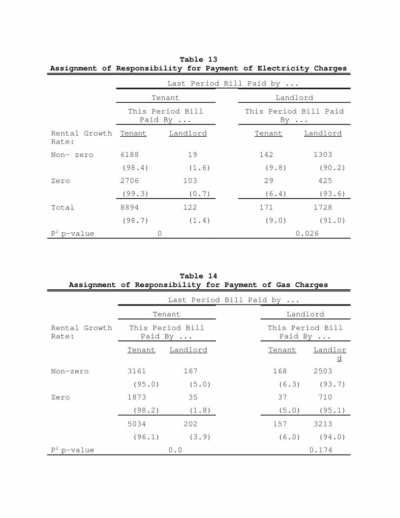
Table 13Assignment of Responsibility for Payment of Electricity Charges
Last Period Bill Paid by ...
Tenant Landlord
This Period BillPaid By ...
This Period Bill PaidBy ...
Rental GrowthRate:
Tenant Landlord Tenant Landlord
Non- zero 6188 19 142 1303
(98.4) (1.6) (9.8) (90.2)
Zero 2706 103 29 425
(99.3) (0.7) (6.4) (93.6)
Total 8894 122 171 1728
(98.7) (1.4) (9.0) (91.0)
P2 p-value 0 0.026
Table 14Assignment of Responsibility for Payment of Gas Charges
Last Period Bill Paid by ...
Tenant Landlord
Rental GrowthRate:
This Period BillPaid By ...
This Period BillPaid By ...
Tenant Landlord Tenant Landlord
Non-zero 3161 167 168 2503
(95.0) (5.0) (6.3) (93.7)
Zero 1873 35 37 710
(98.2) (1.8) (5.0) (95.1)
5034 202 157 3213
(96.1) (3.9) (6.0) (94.0)
P2 p-value 0.0 0.174

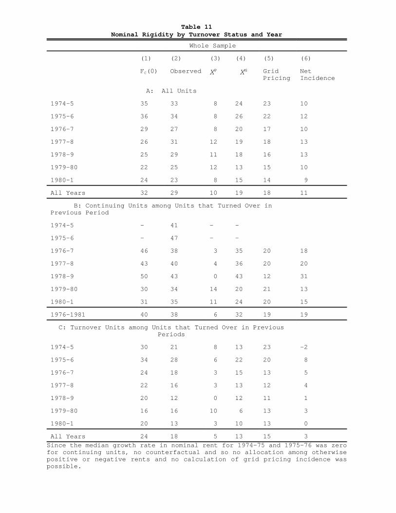
Table 11Nominal Rigidity by Turnover Status and Year
Whole Sample
(1) (2) (3) (4) (5) (6)
FC(0) Observed XP XN Grid Pricing
NetIncidence
A: All Units
1974-5 35 33 8 24 23 10
1975-6 36 34 8 26 22 12
1976-7 29 27 8 20 17 10
1977-8 26 31 12 19 18 13
1978-9 25 29 11 18 16 13
1979-80 22 25 12 13 15 10
1980-1 24 23 8 15 14 9
All Years 32 29 10 19 18 11
B: Continuing Units among Units that Turned Over inPrevious Period
1974-5 - 41 - -
1975-6 - 47 - -
1976-7 46 38 3 35 20 18
1977-8 43 40 4 36 20 20
1978-9 50 43 0 43 12 31
1979-80 30 34 14 20 21 13
1980-1 31 35 11 24 20 15
1976-1981 40 38 6 32 19 19
C: Turnover Units among Units that Turned Over in PreviousPeriods
1974-5 30 21 8 13 23 -2
1975-6 34 28 6 22 20 8
1976-7 24 18 3 15 13 5
1977-8 22 16 3 13 12 4
1978-9 20 12 0 12 11 1
1979-80 16 16 10 6 13 3
1980-1 20 13 3 10 13 0
All Years 24 18 5 13 15 3
Since the median growth rate in nominal rent for 1974-75 and 1975-76 was zerofor continuing units, no counterfactual and so no allocation among otherwisepositive or negative rents and no calculation of grid pricing incidence waspossible.
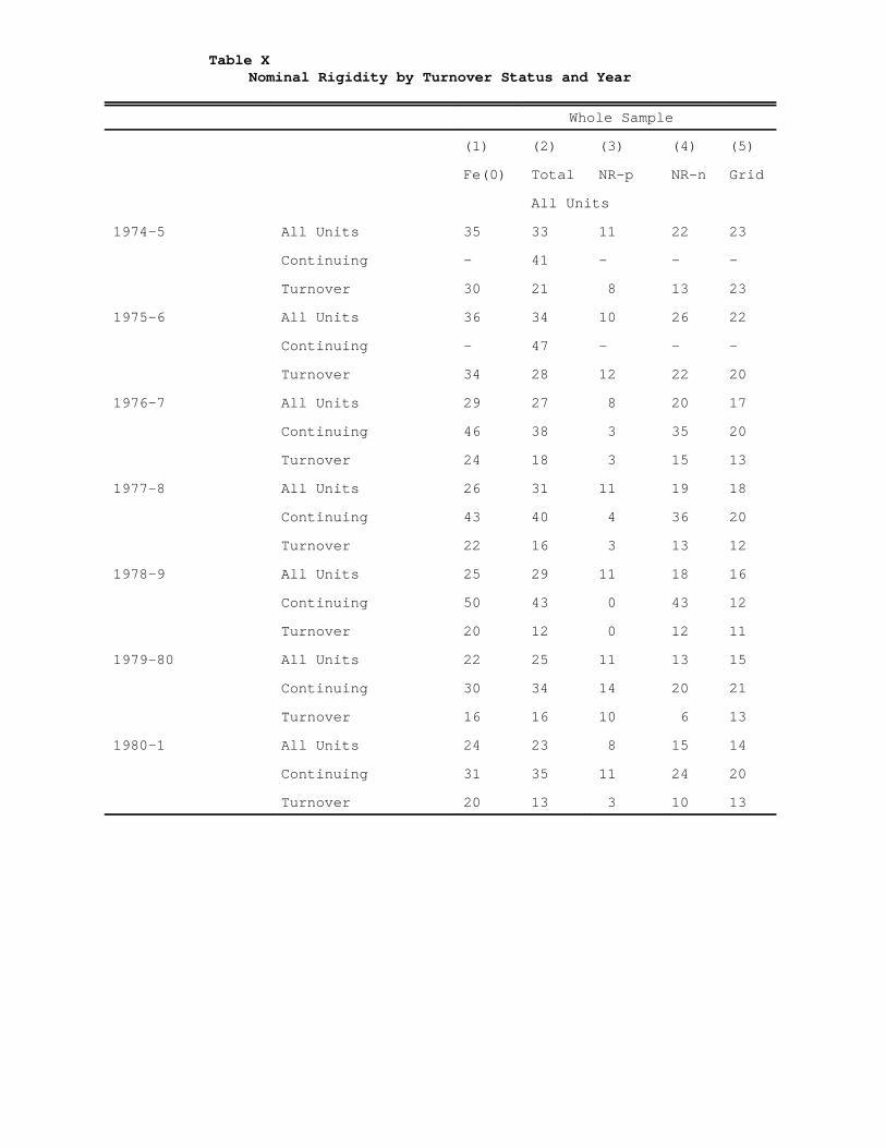
Table XNominal Rigidity by Turnover Status and Year
Whole Sample
(1) (2) (3) (4) (5)
Fe(0) Total NR-p NR-n Grid
All Units
1974-5 All Units 35 33 11 22 23
Continuing - 41 - - -
Turnover 30 21 8 13 23
1975-6 All Units 36 34 10 26 22
Continuing - 47 - - -
Turnover 34 28 12 22 20
1976-7 All Units 29 27 8 20 17
Continuing 46 38 3 35 20
Turnover 24 18 3 15 13
1977-8 All Units 26 31 11 19 18
Continuing 43 40 4 36 20
Turnover 22 16 3 13 12
1978-9 All Units 25 29 11 18 16
Continuing 50 43 0 43 12
Turnover 20 12 0 12 11
1979-80 All Units 22 25 11 13 15
Continuing 30 34 14 20 21
Turnover 16 16 10 6 13
1980-1 All Units 24 23 8 15 14
Continuing 31 35 11 24 20
Turnover 20 13 3 10 13

Table 4bNominal Rigidity by Turnover Status and Year
1974-5 1975-6 1976-7
Neg. Zero Pos. Neg. Zero Pos. Neg. Zero Pos.
C 9 40 51 10 40 50 9 35 56
T 15 19 67 11 21 68 9 14 77
N 15531707 1594
1977-8
1978-9
1979-80
C 6 40 54 7 37 56 8 32 60
T 8 12 80 7 12 81 9 12 79
N 15071612
1644
1980-1
C 8 30 61
T 9 10 81
N 1607
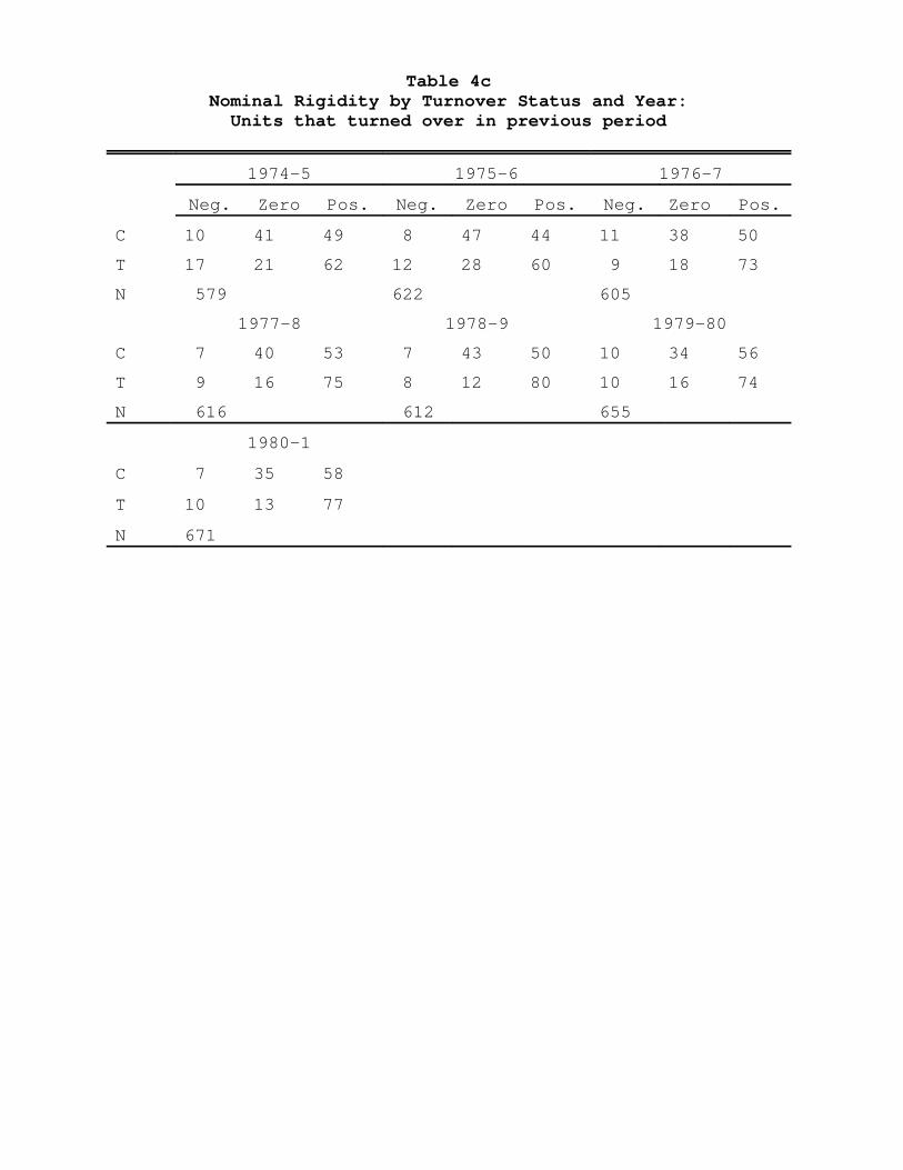
Table 4cNominal Rigidity by Turnover Status and Year:Units that turned over in previous period
1974-5 1975-6 1976-7
Neg. Zero Pos. Neg. Zero Pos. Neg. Zero Pos.
C 10 41 49 8 47 44 11 38 50
T 17 21 62 12 28 60 9 18 73
N 579 622 605
1977-8 1978-9 1979-80
C 7 40 53 7 43 50 10 34 56
T 9 16 75 8 12 80 10 16 74
N 616 612 655
1980-1
C 7 35 58
T 10 13 77
N 671
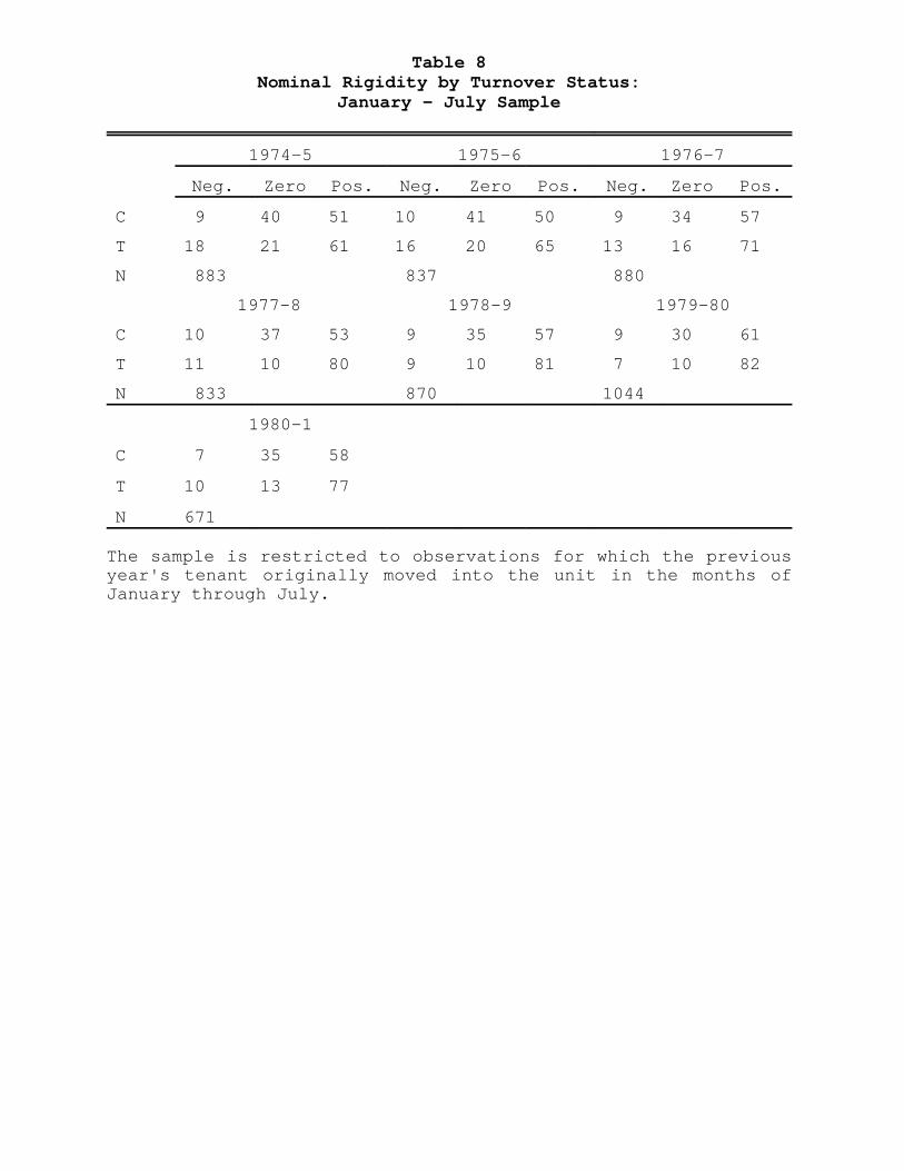
Table 8Nominal Rigidity by Turnover Status:
January - July Sample
1974-5 1975-6 1976-7
Neg. Zero Pos. Neg. Zero Pos. Neg. Zero Pos.
C 9 40 51 10 41 50 9 34 57
T 18 21 61 16 20 65 13 16 71
N 883 837 880
1977-8 1978-9 1979-80
C 10 37 53 9 35 57 9 30 61
T 11 10 80 9 10 81 7 10 82
N 833 870 1044
1980-1
C 7 35 58
T 10 13 77
N 671
The sample is restricted to observations for which the previousyear's tenant originally moved into the unit in the months ofJanuary through July.