
MT4514: Graph Theory - University of St...
59
MT4514: Graph Theory Colva M. Roney-Dougal February 5, 2009
Transcript of MT4514: Graph Theory - University of St...

MT4514: Graph Theory
Colva M. Roney-Dougal
February 5, 2009
Contents
1 Introduction 31 About the course . . . . . . . . . . . . . . . . . . . . . . . . . . . . . 32 Some introductory examples . . . . . . . . . . . . . . . . . . . . . . . 3
2 Basic definitions and isomorphism 81 Some definitions . . . . . . . . . . . . . . . . . . . . . . . . . . . . . 82 Isomorphism . . . . . . . . . . . . . . . . . . . . . . . . . . . . . . . 93 Some families of graphs . . . . . . . . . . . . . . . . . . . . . . . . . 114 Degree sequences . . . . . . . . . . . . . . . . . . . . . . . . . . . . . 11
3 Paths on graphs 151 Definitions . . . . . . . . . . . . . . . . . . . . . . . . . . . . . . . . . 152 Eulerian circuits . . . . . . . . . . . . . . . . . . . . . . . . . . . . . 153 Hamiltonian Circuits . . . . . . . . . . . . . . . . . . . . . . . . . . . 18
4 Planarity and Colouring 211 Euler’s Formula and Kuratowski’s Theorem . . . . . . . . . . . . . . 212 Regular Polyhedra . . . . . . . . . . . . . . . . . . . . . . . . . . . . 233 Colouring Planar Graphs . . . . . . . . . . . . . . . . . . . . . . . . 244 Colouring non-planar graphs . . . . . . . . . . . . . . . . . . . . . . 275 The chromatic polynomial . . . . . . . . . . . . . . . . . . . . . . . . 286 The chromatic number of the line and plane . . . . . . . . . . . . . . 31
5 Marriage, Matchings and Connectivity 331 Hall’s Marriage Theorem . . . . . . . . . . . . . . . . . . . . . . . . . 332 Edge colourings of graphs . . . . . . . . . . . . . . . . . . . . . . . . 343 Factorisation of graphs . . . . . . . . . . . . . . . . . . . . . . . . . . 364 Connectivity of graphs . . . . . . . . . . . . . . . . . . . . . . . . . . 38
6 Trees 421 Characterisation of Trees . . . . . . . . . . . . . . . . . . . . . . . . 422 Counting Trees . . . . . . . . . . . . . . . . . . . . . . . . . . . . . . 43
7 Ramsey Theory 481 Graphs with no triangles . . . . . . . . . . . . . . . . . . . . . . . . . 482 Ramsey Numbers . . . . . . . . . . . . . . . . . . . . . . . . . . . . . 493 Ramsey numbers for several colours . . . . . . . . . . . . . . . . . . 51
8 Adjacency matrices 531 Definitions and basic results . . . . . . . . . . . . . . . . . . . . . . . 532 Eigenvalues . . . . . . . . . . . . . . . . . . . . . . . . . . . . . . . . 543 The eigenvalue method . . . . . . . . . . . . . . . . . . . . . . . . . . 55
2

Chapter 1
Introduction
1. About the course
The course will not be solely based on a single book. Therefore, the best studysource will be the lecture notes. Some useful texts are:
1. Robin Wilson, Introduction to Graph Theory
2. Robin Wilson and John Watkins, Graphs – an Introductory Approach.
3. Frank Harary, Graph Theory.
4. Norman Biggs, Discrete Mathematics
All these books, as well as all tutorial sheets and solutions, will be available inMathematics/Physics library on short loan. Also, any other book containing in itstitle the words such as ‘graph theory’, ‘discrete mathematics’, ‘combinatorics’ islikely to contain material relevant to the course.
It will be useful to bring coloured pens or pencils to lectures, although I’ve hadto do these notes in black and white.
2. Some introductory examples
Graphs are a very useful way of recording information about objects and relation-ships between pairs of objects. A graph consists of a set V of vertices or points anda collection E of edges joining some of the pairs of points.
In this introduction we’ll look at a range of examples to indicate the flavour andvariety of the topic. Graph theory goes back to ancient Greek times, with the studyof the 5 regular platonic solids, but it really started with the following problem.
Example 2.1. Konigsberg Bridge problem. Consider this town plan of Konigsberg(now Kaliningrad) in East Prussia. The river Pregel runs through the middle oftown, and a set of 7 bridges links the banks and two islands in the river. Theproblem is to find a walk through the town that begins and ends at the same place,crossing each bridge exactly once.
3

4 Colva M. Roney-Dougal
Euler in 1736 realised that we can simplify the problem by representing it with thisgraph, with one edge for each bridge, and vertices representing each island and eachbank.
The problem now is to find a path around the graph which begins and ends at thesame vertex and follows each edge exactly once. Looking at this graph, Euler wasable to show that the problem has no solution.
Example 2.2. Knight’s tour. Given an n ×m chessboard, we ask whether it’spossible to find a route for a knight that visits each square on the board exactlyonce. We represent the 3× 4 chessboard with a graph like this, with one vertex foreach square, and edges linking squares that a knight can move between in a singlego:
A knight’s tour corresponds to finding a path on the graph that visits each vertexexactly once. Euler considered the problem of the 8× 8 board.
Example 2.3. Logical games. Consider a game such as noughts and crosses,where there is no element of chance. We can draw a graph whose vertices representall possible positions during a game. The edges of the graph connect each positionto those positions which can be reached by a single move.
A strategic analysis of the game is possible by looking at the paths in the graph.
Example 2.4. Paths on a die. To find a circuit on a die visiting each face exactlyonce we consider this graph:

Graph Theory 5
There is one vertex for each face, and an edge connecting adjacent faces. We wantto find a closed circuit on the graph visiting each vertex exactly once. One solutionis 1, 3, 6, 5, 4, 2, 1.Problem: How many such paths are there?
Example 2.5. Maps. Information on maps can often be presented with a graph,where edges may also be labelled with distances. An example with no distances isthe London underground map. Here we give a more local map with distances:
A famous problem connected with graphs representing maps is the TravellingSalesman Problem: find the shortest path that visits each town at least once andreturns to the start.
Example 2.6. People at a party. Given a group of six people, we can alwaysfind either three who all know each other or three who don’t know each other. Wecan represent this with this graph, with one vertex for each person. We put a rededge between two vertices if the two people know each other, and a green edge ifthey do not.
The previous example is equivalent to the following:
Theorem 2.7. Let (V,E) be a graph with six vertices and an edge between everypair of vertices that is either red or green. Then (V,E) contains either a red triangleor a green triangle.
Proof. Let v ∈ V be any vertex. Then v has five adjacent edges, so either atleast three red edges or at least three green edges leave v. Without loss of generalitywe may assume that at least three red edges leave v, and that they join v to verticesv1, v2, v3:

6 Colva M. Roney-Dougal
Now consider the edges v1v2, v1v3 and v2v3. If any of them, say vivj , is red thenwe have found a red triangle vvivj . If none of them is red then we have found agreen triangle v1v2v3. �
Similarly, in a group of 18 people there are 4 mutual acquaintances or non-acquaintances, and we know that in a group of 17 people there may not be sucha group of four people. In a group of 49 people there are 5 mutual acquaintancesor non-acquaintances, but we do not know if 49 is the smallest number thatguarantees the existence of 5 acquaintances or non-acquaintances: the smallestsuch number may be as low as 43.
Example 2.8. A puzzle: missionaries and cannibals. Two missionaries andtwo cannibals need to cross a river from west to east in a boat holding at most twopeople. To avoid being eaten, if there are any missionaries on a bank then theremust be at least as many missionaries as cannibals.
We make a graph whose vertices are pairs (M,C) describing how many mission-aries and cannibals are on the west bank of the river. We put arrows of one typeindicating boat trips from west to east, and of another type to indicate boat tripsfrom east to west.
To find a solution we need to find a path of alternating types of arrows (as we mustalways bring the boat back from the other side), that starts with the vertex (2, 2)and ends with the vertex (0, 0). A possible solution is:
(2, 2) → (1, 1) → (2, 1) → (0, 1) → (0, 2) → (0, 0).
That is, one missionary and one cannibal cross, the missionary comes back, thentwo missionaries cross, then the cannibal comes back, then both cannibals cross.
Example 2.9. Further examples include
• The internet: vertices for computers and edges for connections, maybe labelledby their bandwidth.
• Graphs of groups, for example the automorphism group of the following graphis A4:

Graph Theory 7
• Chemistry: diagrams of saturated hydrocarbons.
• Management structures.
• Network flows, such as the national grid, the water supply.
Chapter 2
Basic definitions and isomorphism
In this chapter we give some of the formal definitions of graph theory, and establishsome elementary properties of graphs.
1. Some definitions
Definition 1.1. A simple graph G consists of a finite set V of vertices (also calledpoints or nodes) and a set E of edges such that each edge joins a pair of vertices inV . More formally, a simple graph is a pair (V,E) where V is a finite set and E isa set of subsets of V , each of size 2.
When V and E are finite sets we write |G| or |V | to denote the number ofvertices of G. The graph G is finite when V and E are finite. We denote the edgejoining vi and vj by vivj . Note that vivj = vjvi as the edges of a graph do not havea direction.
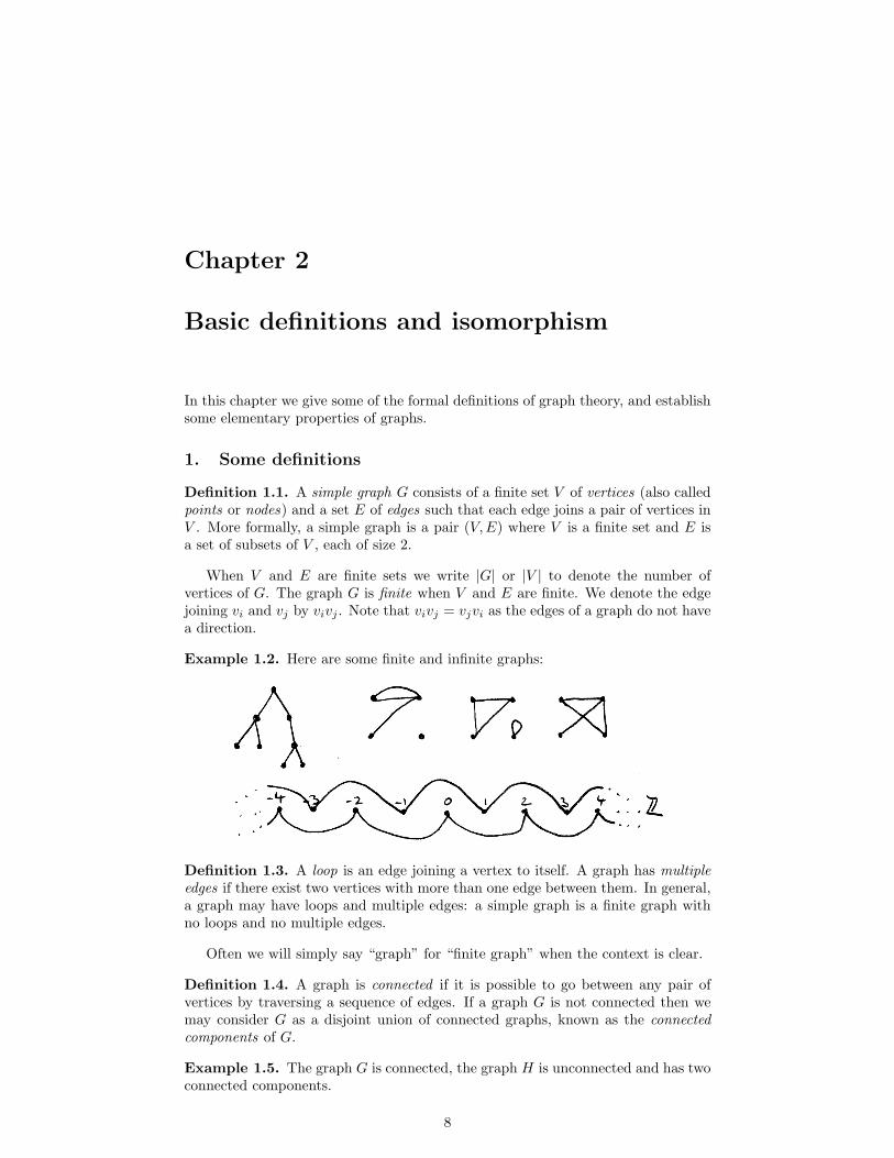
Example 1.2. Here are some finite and infinite graphs:
Definition 1.3. A loop is an edge joining a vertex to itself. A graph has multipleedges if there exist two vertices with more than one edge between them. In general,a graph may have loops and multiple edges: a simple graph is a finite graph withno loops and no multiple edges.
Often we will simply say “graph” for “finite graph” when the context is clear.
Definition 1.4. A graph is connected if it is possible to go between any pair ofvertices by traversing a sequence of edges. If a graph G is not connected then wemay consider G as a disjoint union of connected graphs, known as the connectedcomponents of G.
Example 1.5. The graph G is connected, the graph H is unconnected and has twoconnected components.
8

Graph Theory 9
Definition 1.6. Two vertices v1, v2 ∈ V are adjacent if there is an edge joining v1
to v2. The degree or valency of a vertex v is the number of edges that have one endat v: each loop at a vertex v contributes 2 to the valency of v. The graph is regularif all vertices have the same degree.
Example 1.7. This graph has vertices labelled by their valencies.
Lemma 1.8 (Handshaking lemma) The sum of all of the degrees of all verticesof a finite graph is even.
Proof. This is clear since each edge contributes 1 to the degree of two vertices,or 2 to a single one. �
Definition 1.9. A graph G is planar if G can be drawn in the plane (i.e. on a flatpiece of paper) without the edges crossing.
Example 1.10. G is a planar graph, H is not.
2. Isomorphism
The way that we draw a graph, or the nature of the set V , does not matter when weare studying graphs. Consider the bijection φ between the following graphs, whichshows that they are essentially the same:
10 Colva M. Roney-Dougal
Definition 2.1. The simple graphs G = (V,E) and G′ = (V ′, E′) are isomorphicif there exists a bijection φ : V → V ′ such that v1v2 is an edge of E if and only ifφ(v1)φ(v2) is an edge of E′. If an isomorphism exists then we write G ∼= G′.
Two graphs that are isomorphic share many properties in an obvious way:
• They have the same number of vertices.
• They have the same number of edges.
• Corresponding vertices have equal valencies.
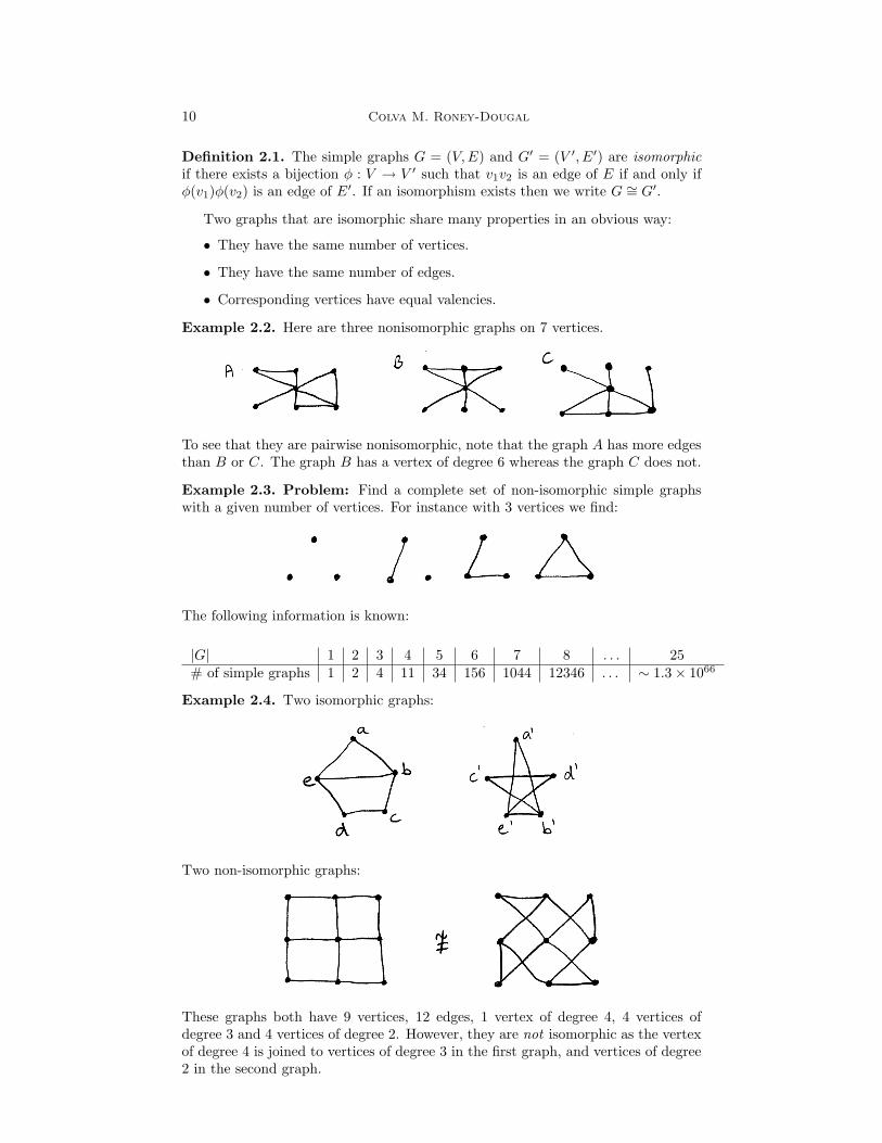
Example 2.2. Here are three nonisomorphic graphs on 7 vertices.
To see that they are pairwise nonisomorphic, note that the graph A has more edgesthan B or C. The graph B has a vertex of degree 6 whereas the graph C does not.
Example 2.3. Problem: Find a complete set of non-isomorphic simple graphswith a given number of vertices. For instance with 3 vertices we find:
The following information is known:
|G| 1 2 3 4 5 6 7 8 . . . 25# of simple graphs 1 2 4 11 34 156 1044 12346 . . . ∼ 1.3× 1066
Example 2.4. Two isomorphic graphs:
Two non-isomorphic graphs:
These graphs both have 9 vertices, 12 edges, 1 vertex of degree 4, 4 vertices ofdegree 3 and 4 vertices of degree 2. However, they are not isomorphic as the vertexof degree 4 is joined to vertices of degree 3 in the first graph, and vertices of degree2 in the second graph.

Graph Theory 11
3. Some families of graphs
Definition 3.1. The complete graph on n vertices is denoted Kn, and is the graphon n vertices where every pair of distinct vertices is joined by an edge.
Every vertex of Kn has degree (n− 1) so there are n(n− 1)/2 edges.
Definition 3.2. A bipartite graph is one where the vertices are divided into twoclasses, R and B say, with the property that every edge has one end in R and theother end in B. For example:
We denote by Km,n the complete bipartite graph with |R| = m and |B| = n andevery vertex of R joined to every vertex of B.
Here are some other kinds of graph.
A tree is a connected graph which contains no circuits.
4. Degree sequences
Definition 4.1. Let G be a simple graph. The degree sequence of G is the list ofdegrees of the vertices of G, usually in decreasing order.
For instance the following graph has degree sequence 4, 3, 3, 2, 2:

12 Colva M. Roney-Dougal
Given a sequence of non-negative integers, how can we tell whether there is agraph with that as a degree sequence? For example, 6, 6, 5, 5, 3, 3, 3, 3 is the degreesequence of a simple graph, but 6, 6, 5, 5, 2, 2, 2, 2 is not.
Theorem 4.2. The following are necessary conditions for d1, . . . , dv to be a degreesequence.
1. The sum of the di is even.
2. We have di ≤ v − 1 for 1 ≤ i ≤ v.
3. At least two vertices have equal degree.
Proof.
1. The sum of the degrees is twice the number of edges (recall the HandshakingLemma, Chapter 1, 1.8).
2. In a simple graph, each vertex can be joined to at most v − 1 others.
3. Suppose not, then by (2) the degrees must be v − 1, v − 2, . . . , 1, 0. Thereforethe vertex of degree v − 1 must be joined to all other vertices, including thatof degree 0.
�
Remark 4.3. Nonisomorphic graphs can have the same degree sequences. Forexample consider the following two graphs:
They both have degree sequence 3, 3, 2, 2, 2 but are nonisomorphic since the firstcontains a triangle but the other does not.
Lemma 4.4. Let a graph G have the degree sequence
s ≥ v1 ≥ v2 ≥ · · · ≥ vs ≥ d1 ≥ · · · ≥ dk
and vertices S, Vi and Dj of corresponding degrees. Then there exists a graph Hwith the same degree sequence such that S is joined to V1, V2, . . . , Vs.
Proof. Suppose that in G, the vertex S is not joined to at least one of the Vi.Then S must be joined to at least one Dj . Recall that vi ≥ dj . If vi = dj then wemay swap the labels Vi and Dj on the graph to get a graph with S joined to onemore of the Vi and one less of the Dj vertices.
Otherwise vi > dj . Then there is some vertex W joined to Vi but not to Dj .Consider the graph G′ obtained from G by removing edges SDj and WVi andreplacing them by edges SVi and WDj :
Graph Theory 13
Then none of the vertex degrees have changed, but S is joined to one more ofthe Vi and one fewer of the Dj vertices. In particular, G′ has degree sequence (1),so we may replace G by G′.
We may then repeat these two processes to get a graph H with S joined to allof the Vi, proving the lemma. �
Theorem 4.5. Consider the sequences
s, v1, v2, . . . , vs, d1, . . . , dk (1)
andv1 − 1, v2 − 1, . . . , vs − 1, d1, d2, . . . , dk (2),
where (1) is written in decreasing order, vi ≥ 1, and vi, di ∈ N for all i. Then (1)is a degree sequence of a simple graph if and only if (2) is the degree sequence of asimple graph.
For example 6, 6, 5, 5, 2, 2, 2, 2 is a degree sequence if and only if 5, 4, 4, 2, 1, 1, 1is a degree sequence, if and only if 3, 3, 1, 1, 0, 0 is a degree sequence, if and only if2, 0, 0, 0, 0 is a degree sequence. Since this final sequence is clearly not the degreesequence of a simple graph, none of the preceding ones are.
Proof.⇐: If (2) is the degree sequence of some graph then by adding one further vertex Sjoined to the vertices of degree v1 − 1, v2 − 1, . . . , vs − 1 we get a graph with degreesequence (1).⇒: Let G have degree sequence (1) and write S, Vi, Dj for the vertices with degreess, vi and dj respectively. The graph H given by Lemma 4.4 has the same degreesequence as G, and in H the vertex S is joined to V1, . . . , Vs. By removing the vertexS and edges SV1, SV2, . . . , SVs we get a graph with degree sequence (2). �
Example 4.6. 1. The sequence 4, 3, 3, 2, 1 is not a degree sequence since thesum is odd.
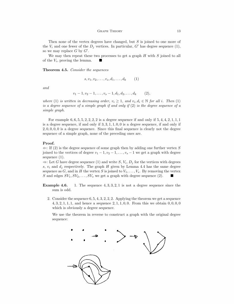
2. Consider the sequence 6, 5, 4, 3, 2, 2, 2. Applying the theorem we get a sequence4, 3, 2, 1, 1, 1, and hence a sequence 2, 1, 1, 0, 0. From this we obtain 0, 0, 0, 0which is obviously a degree sequence.
We use the theorem in reverse to construct a graph with the original degreesequence:

14 Colva M. Roney-Dougal
3. Consider the sequence 7, 7, 7, 6, 6, 5, 2, 2, 1, 1. Applying the theorem we get asequence 6, 6, 5, 5, 4, 1, 1, 1, 1, then 5, 4, 4, 3, 1, 1, 0, 0, and then 3, 3, 2, 0, 0, 0, 0(∗). There is no graph with degree sequence ∗, as in order for a vertex to havedegree 3 there must be at least four vertices of nonzero degree. Hence by thetheorem there is no graph with the original degree sequence.
4. Consider the sequence 7, 7, 6, 5, 4, 4, 4, 2, 1. Applying the theorem we get asequence 6, 5, 4, 3, 3, 3, 1, 1, which yields 4, 3, 2, 2, 2, 1, 0. In turn we now get2, 1, 1, 1, 1, 0 and then 1, 1, 0, 0, 0. This last sequence is the degree sequence ofa graph with 5 vertices and a single edge, so all of these sequences are degreesequences of simple graphs.

Chapter 3
Paths on graphs
1. Definitions
Throughout this chapter, G will be a finite connected graph.
Definition 1.1. A path on G is a sequence of vertices v1, v2, . . . , vn such that vivi+1
is an edge of G for 1 ≤ i ≤ n − 1. A circuit is a path v1, . . . , vn such that vnv1 isalso an edge.
Example 1.2. In the first graph a circuit is marked, in the second a path is marked.
Definition 1.3. A connected graph is Eulerian if there exists a circuit using everyedge exactly once. It is semi-Eulerian if there is a path including every edge exactlyonce. It is Hamiltonian if there exists a circuit including every vertex exactly once,and semi-Hamiltonian if there exists a path including every vertex exactly once.
Example 1.4. Graph 1 is semi-Eulerian and semi-Hamiltonian. Graph 2 is Eule-rian and Hamiltonian (follow the arrows). Graph 3 is Hamiltonian but not Eulerianor semi-Eulerian. Do you recognise graph 3?
2. Eulerian circuits
Theorem 2.1 (Euler’s Theorem) A connected graph is Eulerian if and only ifevery vertex has even degree.
Proof.⇒: A circuit goes into and then out of each vertex an unknown number of times,each time using two edges (one to get in and then one to get out). Thus there arean even number of edges incident to each vertex.
15

16 Colva M. Roney-Dougal
⇐: Start at any vertex v and walk around the graph using no edge more than once.Since each vertex has even degree, we will always have a way out of each vertexuntil we return to vertex v. Call this circuit C1. If C1 contains all of the edges thenwe are done. If not, the remaining edges are such that an even number of then areincident to each vertex, so we may repeat our initial process to get further circuitsC2, C3, . . . , Ck, until all of the edges are used in exactly one of the Ci.
If k > 1 we now join up the circuits to form a single circuit. Since the graph isconnected, C1 must have a vertex in common with at least one Cj for j > 1. Wemay amalgamate C1 and Cj to form a single circuit by rerouting at the commonvertex:
Repeating this we may combine C1, . . . , Ck into a single path including each edgeexactly once. �
Example 2.2. In the following graph, we note that all vertices have even degree,so we may find an Eulerian circuit.
In the final graph we amalgamate C1, C2, C3 to make a single circuit.
Example 2.3. It is immediate from Euler’s theorem that the Bridges of Konigsberggraph from Chapter 1, Example 2.1 has no Eulerian path.
Corollary 2.4. A connected graph is semi-Eulerian but not Eulerian if and only ifit has exactly two vertices of odd degree.
Proof. We start by noting that any Eulerian path must begin at one odd degreevertex and end at another.⇒: Except for the vertices at the start and finish of the path, every time we go intoa vertex along one edge, we go out along another edge. Therefore each time thatwe visit an intermediate vertex we account for two edges. Thus every vertex otherthan the first and last must have even degree.⇐: Let v0, v1 be the two vertices of odd degree in a graph G. Add an edge joiningv0 and v1 to get a graph G′ such that every vertex of G′ has even degree. By Euler’stheorem, G′ has an Eulerian circuit. Removing the edge v0v1 leaves an Eulerianpath on G which begins at v0 and ends at v1, as required. �
Example 2.5. The first of these graphs is Eulerian. The second, with one extraedge, is semi-Eulerian.

Graph Theory 17
Algorithm 2.6. Fleury’s algorithm This is an algorithm for finding Eulerianpaths or circuits in a graph. Given a graph with either two or no vertices of odddegree, start at any vertex in the Eulerian case and at one of the two odd degreevertices in the semi-Eulerian case. Walk around the graph choosing new edges withthe proviso that you never take an edge if it would split the remaining edges intotwo disconnected graphs, and that you don’t use the last edge into the start vertextoo soon.
Example 2.7. Consider the first graph of Example 2.5:

18 Colva M. Roney-Dougal
Remark 2.8. Fleury’s algorithm is common sense, in that if we end up with twodisconnected blocks of edges we clearly cannot complete a circuit.
3. Hamiltonian Circuits
Unlike the Eulerian case, where Euler’s Theorem 2.1 completely classifies the Eule-rian graphs, there is no simple criterion which guarantees the existence of a Hamilto-nian circuit. Many puzzles and problems require one to find a Hamiltonian path, forinstance the Knight’s Tour of Chapter 1, Example 2.2 and the Travelling Salesmanproblem.
Example 3.1. Hamilton’s Round the World ProblemCan you find a Hamiltonian circuit visiting all vertices of a dodecahedron? First wesketch a dodecahedron, which has 20 vertices, 12 pentagonal faces, and 30 edges.Then we give an isomorphic graph to consider:
One can see a Hamiltonian circuit for this graph relatively easily. However, a smallchange gives the following graph, which has no Hamiltonian path or circuit:

Graph Theory 19
To see this, note that although this graph has the same number of vertices andedges as the previous one, to visit the vertices of degree two we must go around themiddle ring of edges. But now any circuit cannot include both the inner and outerrings.
Remark 3.2. In general, one has to argue in a systematic way to show that agraph is not Hamiltonian, or to find a Hamiltonian circuit.
Example 3.3. The Petersen GraphThe Petersen graph is not Hamiltonian.
To prove this, note that up to symmetry there are three ways of passing from theinner to the outer pentagon. In picture (a) we pass at adjacent vertices, in (b) wepass at non-adjacent vertices, and in (c) we pass twice from the inner to the outerpentagon. The passing edges are the non-dotted ones.
In each case, we are forced to traverse certain other edges to guarantee visiting eachvertex. These are the dotted edges. In each case it follows that we cannot completethe circuit.
Intuitively, given a graph, if it has many edges then it is more likely to have aHamiltonian circuit. We formalise this as follows:
Theorem 3.4 (Dirac’s theorem) Let G be a simple graph with n ≥ 3 verticessuch that every vertex has degree at least n/2. Then G has a Hamiltonian circuit.
Proof. We assume that G is a graph with every vertex of degree at least n/2that is not Hamiltonian, and derive a contradiction.
By adding as many edges as possible without making the graph Hamiltonian,we may assume that G is maximal, in the sense that it is non-Hamiltonian butthe addition of any further edges will make it Hamiltonian. Since adding edgesdoesn’t alter the number of vertices, and the complete graph is Hamiltonian, thisassumption is safe.
Let v, w be any pair of non-adjacent vertices of G. There must be a path fromv to w which visits all vertices once, since adding the edge vw would create aHamiltonian circuit, from which we can remove the edge vw. Label the vertices inthis path v = v1, v2, . . . , vn = w.

20 Colva M. Roney-Dougal
Let R be the set of vertices joined to v1, so |R| ≥ n/2, and let B be the set ofvertices that are one before the vertices in R as we go along the path v1, v2, . . . , vn.Note that some vertices may be in both B and R. Then |B| = |R| ≥ n/2 andv1 ∈ B (as v1 is one before v2, and v1v2 is an edge in the path).
The vertex vn is joined to at least n/2 of the n − 2 vertices v2, v3, . . . , vn−1, asvn is not joined to v1 or itself. Since v1 ∈ B and vn 6∈ B, at least n/2 − 1 of thevertices v2, v3, . . . , vn−1 are in B. Since n/2+(n/2−1) > n−2 there exists at leastone vertex vi in v2, v3, . . . , vn−1 that is both in B and joined to vn.
Therefore we have a Hamiltonian circuit v1, v2, . . . , vi, vn, vn−1, vn−2, . . . , vi+1, v1,a contradiction. �
Remark 3.5. Dirac’s theorem does not give a necessary condition. For instancethe cycle with 6 vertices has all vertices of degree 2 (which is less than 6/2) and yethas a Hamiltonian circuit.
A minor modification of the proof of Dirac’s theorem allows one to prove thefollowing:
Theorem 3.6 (Ore’s Theorem) Let G be a simple graph with n ≥ 3 verticessuch that for all non-adjacent vertices v and w we have Degree(v)+Degree(w) ≥ n.Then G has a Hamiltonian circuit.

Chapter 4
Planarity and Colouring
1. Euler’s Formula and Kuratowski’s Theorem
Definition 1.1. A graph G is planar if it can be drawn in the plane without edgescrossing.
Example 1.2. The graph K4 (a) is planar because it is isomorphic to the graph(b) and this second graph has no crossing edges.
We call both graphs planar.
Definition 1.3. The faces of a planar graph are the regions into which the edgesdivide the plane, when the graph is drawn with no crossing edges. We alwaysinclude the unbounded or exterior face.
Example 1.4. The following graph has six faces:
Given a planar graph, we write v, e, f for the number of vertices, edges and facesrespectively. So this graph has v = 6, e = 10 and f = 6.
Theorem 1.5 (Euler’s formula) In every connected planar graph v− e + f = 2.
Proof. We prove this by induction on e.Base case: The connected graph with no edges consists of a single vertex. It has
v = 1, e = 0 and f = 1 so the theorem holds.Inductive step: Assume that the theorem holds for every planar connected graph
with at most n edges. Let G have n+1 edges. Then either G is a tree or G containsa circuit. We consider the two cases separately.
If G is a tree then by removing any edge at the end of a “branch”, along withits terminal vertex, we get a connected graph with n edges.
21

22 Colva M. Roney-Dougal
The value of v is decreased by 1, the value of e is decreased by 1, and the value off is unchanged. So v − e + f is unchanged, and so v − e + f = 2 by the inductivehypothesis and the theorem holds for G.
If G is not a tree, and so contains a circuit, we consider the effect of removingan edge that lies in a circuit, to get a connected graph with n edges.
The value of v is unchanged, e is decreased by 1, and f is decreased by 1 (since twofaces have been merged). So v − e + f is unchanged, and so v − e + f = 2 by theinductive hypothesis and the theorem holds for G.
Therefore the result follows for all e by induction. �
Remark 1.6. Euler’s formula is also valid for graphs drawn on a sphere.
Corollary 1.7. The complete graph K5 is not planar.
Proof. The complete graph K5 has
v = 5 and e =(
52
)= 10.
Therefore by Theorem 1.5 we must have f = 2− v + e = 7 if K5 is planar.The boundary of any face is a circuit. The circuit cannot have a single vertex
as K5 is simple so has no loops. It also cannot have precisely two vertices as K5 issimple so has no multiple edges. Therefore the boundary of each face contains atleast three vertices, and hence at least three edges.
Since each edge separates two faces we have e ≥ 3f/2, that is 10 ≥ 21/2, acontradiction. �
Corollary 1.8. The complete bipartite graph K3,3 is not planar.
Proof. The graph K3,3 has
v = 6 and e = 3× 3 = 9.
Therefore if K3,3 can be drawn in the plane then Theorem 1.5 gives f = 2−v+e = 5.However, since K3,3 is bipartite each face is bounded by at least four edges. Eachedge separates 2 faces, giving e ≥ 4f/2, which gives 9 ≥ 10, a contradiction. �
Remark 1.9. The graphs K3,3 and K5 are the two “basic” non-planar graphs.
Corollary 1.10. Every planar, connected simple graph has at least one vertex ofdegree less than 6.
Proof. Suppose all vertices have degree at least 6. Each edge ends in two vertices,so e ≥ 6v/2 = 3v. However, by Corollary 1.16 we have e ≤ 3v− 6 so 3v ≤ 3v− 6, acontradiction. �

Graph Theory 23
Exercise 1.11. In fact, every such graph with at least four vertices has at leastfour vertices of degree at most 5. Prove this.
Definition 1.12. A subgraph of a graph G is any graph that can be produced fromG by removing edges and vertices. Two graphs G1 and G2 are homeomorphic ifthere exists a graph G such that both G1 and G2 may be produced from G byputting additional vertices of degree 2 along the edges of G. Note that any graphis homeomorphic to itself.
Example 1.13. The first graph is homeomorphic to K3,3, the second is a subgraphof K3,3.
Theorem 1.14 (Kuratowski’s Theorem) A finite connected graph is planar ifand only if it contains no subgraph that is homeomorphic to K3,3 or K5.
Less formally: A finite connected graph G is non-planar if and only if we canfind 5 or 6 vertices in G that are connected together, possibly via other vertices, asK3,3 or K5.Non–proof: One direction follows from Corollaries 1.7 and 1.8. The other directionis too long to be included in the course – see Chapter 11 of the book by Harary.
Example 1.15. The Petersen graph is non-planar because it has a subgraph thatis homeomorphic to K3,3.
Corollary 1.16. Every planar connected simple graph with v ≥ 3 satisfies e ≤3v − 6.
Proof. Apart from the line of length three (for which v = 3, e = 2 so e ≤ 3v−6 =3), every face of such a graph drawn in the plane is bounded by at least three edges,and every edge is adjacent to at most 2 faces (there is only 1 face around an edgeat the end of a branch). Therefore e ≥ 3f/2. We have
2 = v − e + f ≤ v − e + 2e/3 = v − e/3 ⇒ e ≤ 3v − 6.
�
2. Regular Polyhedra
We may use Euler’s formula 1.5 to show that there are just 5 regular polyhedra, orplatonic solids. This method using Euler’s formula is due to Cauchy in 1813.
Definition 2.1. A polyhedron is convex if it has no inward-bending faces. A con-vex polyhedron is regular if every face is a congruent regular polygon and thearrangement of faces at each vertex is the same.

24 Colva M. Roney-Dougal
Theorem 2.2. There are exactly 5 regular polyhedra.
Proof. Let P be a regular polyhedron with all faces regular p-gons (that is,regular p-sided shapes). Assume that d edges meet at each vertex. We can projectthe edges and vertices of P on to the plane to get a corresponding planar graph G.Each vertex of G has degree d and each face of G has p edges. Then e = vd/2 ande = fp/2, as each edge bounds two faces. Therefore v = 2e/d and f = 2e/p.
By Euler’s formula we have
2 = v − e + f =2e
d− e +
2e
p⇒ 2 + e =
2e
d+
2e
p.
Dividing by 2e we get12
+1e
=1d
+1p.
Therefore, 1/2 < 1/d + 1/p, where d and p are integers with d ≥ 3, p ≥ 3. We have
1/2 < 1/d + 1/p ≤ 1/3 + 1/p
and so 1/6 < 1/p and so p < 6. Similarly, d < 6. Thus
(d, p) ∈ {(3, 3), (3, 4), (4, 3), (3, 5), (5, 3)}.
Case 1 d = p = 3. Then we have 1/e = 1/3 + 1/3 − 1/2, so e = 6. Hencev = 2e/d = 4 and f = 2e/p = 4. This is the tetrahedron, or triangle-based pyramid.
Case 2 d = 3, p = 4. We have 1/e = 1/3 + 1/4 − 1/2 so e = 12. Hencev = 2e/d = 8 and f = 2e/p = 6. This is the cube.
Case 3 d = 4, p = 3. This time we have e = 12, v = 6 and f = 8. This is theoctahedron, made by gluing the bottoms of two square-based pyramids together.
Case 4 d = 3, p = 5. Now we have e = 30, v = 20 and f = 12. This is thedodecahedron; a solid whose surface is made by gluing 12 identical regular pentagonstogether.
Case 5 d = 5, p = 3. This gives e = 30, v = 12, f = 20, corresponding tothe icosahedron; a solid whose surface is made by gluing 20 identical equilateraltriangles together. �
3. Colouring Planar Graphs
In 1852 Guthrie asked whether it is possible to colour every map in the plane withat most four colours so that no two countries with a common boundary are thesame colour.
Remark 3.1. Some maps cannot be coloured with less than four colours, for in-stance

Graph Theory 25
The theorem was first announced as proved true by Kempe in 1879. However,Heawood found an error in the proof in 1890. The theorem was finally proved truein 1976 by Appel and Haken, by one of the first lengthy proofs to use a computer.
The problem can easily be rephrased as a problem of colouring the vertices of agraph.
Definition 3.2. A graph G is k-colourable if we may label its vertices with k coloursso that no two adjacent vertices are of the same colour.
Definition 3.3. The chromatic number of a graph G is the least k for which G isk-colourable. We write χ(G) for the chromatic number of G.
Example 3.4. The following graph is 3-colourable:
It is not 2-colourable because it contains triangles.
Example 3.5. A nontrivial bipartite graph G has χ(G) = 2.
Colouring maps is directly related to colouring graphs.
Definition 3.6. Given a map in the plane, the graph of the map is a graph with avertex in each region, and an edge joining a pair of vertices if and only if the regionshave a common boundary.
Property: Every map in the plane has a simple planar graph.The four colour map theorem is therefore equivalent to:
Theorem 3.7 (The four colour theorem) Every planar simple graph is four-colourable.
The proof of this theorem is very long, instead we prove the following.
Theorem 3.8 (The five colour theorem) Every planar simple graph is five-colourable.

26 Colva M. Roney-Dougal
Proof. We prove this by induction on the number n of vertices.For n ≤ 5 the result is trivial as we can simply colour each vertex a distinct
colour. So assume that the result holds for all graphs with fewer than n vertices.Let G be a planar simple graph with n vertices. Since n > 5 it follows from
Corollary 1.10 that G has a vertex A of degree at most 5. Remove A (and all edgesending at A) to get a new graph G′. Since G′ has n− 1 vertices, we can colour G′
with at most 5 colours by induction.If the degree of A is at most 4, then there is a colour not assigned to any vertex
that is adjacent to A in G, so we can take the colouring for G′ and use this remainingcolour on A to finish the colouring of G.
Therefore we need only consider the case where A has degree 5. Let the neigh-bours of A be a1, a2, a3, a4, a5, numbered to go in a clockwise direction around A.If any two of the ai have the same colour, then there is a spare colour available forA and we are done.
Let i denote the colour of the vertex ai, and write Gij for the subgraph of G\{A}consisting of the vertices with colours i and j, and any edges between them thatare in G. We divide into two cases:
Case 1. a1 and a3 are not joined within G1,3.
Then we may interchange colours 1 and 3 on the part of G1,3 connected to a1 togive a 5-colouring of G \ {A} such that a1 now has colour 3. We now can colour Awith colour 1, as none of its neighbours is coloured 1.
Case 2. a1 and a3 are joined by a path in G1,3.
Then a2 and a4 cannot be joined by a path in G2,4 as G is planar so G2,4 cannotcross G1,3 (and cannot share a vertex with G1,3). Therefore we may proceed as incase 1 to recolour a2 with colour 4, and then colour A with colour 2. �
Remark 3.9. 1. Since K4 is planar there are planar graphs which require 4colours.
2. Colouring graphs on more complicated surfaces is easier. Suppose that westart with a sphere, and glue n “handles” onto it. That is, gluing one handleproduces a torus, gluing two produces a double torus and so on. Then anygraph that can be drawn on a surface with n handles can be coloured with atmost N colours, where
N = b7 +√
1 + 48n
2c,

Graph Theory 27
and bxc is the largest integer that is less than or equal to x. Thus for a toruswe require N = 7 colours. This is best possible as K7 can be drawn on thesurface of the torus without crossings.
4. Colouring non-planar graphs
Colouring questions are also of interest for non-planar graphs, even though thesedo not correspond to maps. We define a k-colouring of a graph G and its chromaticnumber χ(G) as in Definitions 3.2 and 3.3.
Example 4.1. We show how to solve a timetabling problem using graph-colouring.Suppose we have the following requirements:
Student Courses1 A, B2 A, C3 C, D4 B, E5 D, E
We wish to schedule classes so that no student has to be in two places at once. Todo so we draw the following graph G, with one node per course and edges joiningtwo courses if they are taken by the same student.
We see that χ(G) = 3. Colouring the graph G with 3 colours gives a timetablingarrangement with each colour corresponding to a timetabling slot.
We now consider some more general estimates on χ.
Proposition 4.2. Let G be a graph with every vertex of degree at most n for somen, then χ(G) ≤ n + 1.
Proof. Label the vertices of G with v1, . . . , vk in any order. Let the colours bec1, . . . , cn+1. We then use the greedy algorithm to colour the graph: consider thevertices in order v1, . . . , vk, and for each vertex vi use the smallest value of j suchthat cj is not the colour of a neighbouring vertex. Since no vertex has more than nneighbours, there will always be at least one colour available. �
Example 4.3. Here’s a worked example:
Here is a more powerful theorem, whose proof is too hard for this course:
Theorem 4.4 (Brooke’s Theorem) Let G be a graph with all vertices of degreeat most n. Then χ(G) ≤ n unless one of the following holds
28 Colva M. Roney-Dougal
1. A connected component of G is Kn+1 where χ(G) = n + 1.
2. We have n = 2 and a connected component of G is a circuit with an oddnumber of vertices, where χ(G) = 3.
5. The chromatic polynomial
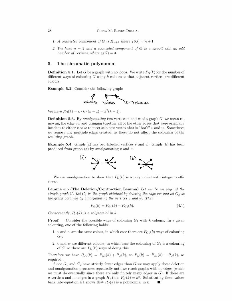
Definition 5.1. Let G be a graph with no loops. We write PG(k) for the number ofdifferent ways of colouring G using k colours so that adjacent vertices are differentcolours.
Example 5.2. Consider the following graph:
We have PG(k) = k · k · (k − 1) = k2(k − 1).
Definition 5.3. By amalgamating two vertices v and w of a graph G, we mean re-moving the edge vw and bringing together all of the other edges that were originallyincident to either v or w to meet at a new vertex that is ”both” v and w. Sometimeswe remove any multiple edges created, as these do not affect the colouring of theresulting graph.
Example 5.4. Graph (a) has two labelled vertices v and w. Graph (b) has beenproduced from graph (a) by amalgamating v and w.
We use amalgamation to show that PG(k) is a polynomial with integer coeffi-cients.
Lemma 5.5 (The Deletion/Contraction Lemma) Let vw be an edge of thesimple graph G. Let G1 be the graph obtained by deleting the edge vw and let G2 bethe graph obtained by amalgamating the vertices v and w. Then
PG(k) = PG1(k)− PG2(k). (4.1)
Consequently, PG(k) is a polynomial in k.
Proof. Consider the possible ways of colouring G1 with k colours. In a givencolouring, one of the following holds:
1. v and w are the same colour, in which case there are PG2(k) ways of colouringG1;
2. v and w are different colours, in which case the colouring of G1 is a colouringof G, so there are PG(k) ways of doing this.
Therefore we have PG1(k) = PG2(k) + PG(k), so PG(k) = PG1(k) − PG(k), asrequired.
Since G1 and G2 have strictly fewer edges than G we may apply these deletionand amalgamation processes repeatedly until we reach graphs with no edges (whichwe must do eventually since there are only finitely many edges in G). If there aren vertices and no edges in a graph H, then PH(k) = kn. Substituting these valuesback into equation 4.1 shows that PG(k) is a polynomial in k. �
Graph Theory 29
Remark 5.6. The chromatic number χ(G) of a graph is the least positive integerk such that PG(k) 6= 0. The deletion/contraction lemma 5.5 gives an algorithmfor chromatic polynomials. We usually just draw diagrams rather than writingequations in PG(k).
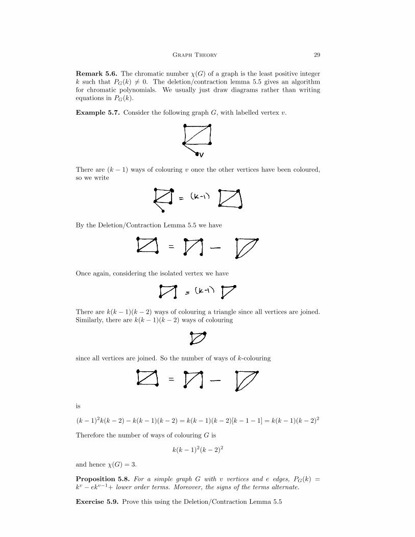
Example 5.7. Consider the following graph G, with labelled vertex v.
There are (k − 1) ways of colouring v once the other vertices have been coloured,so we write
By the Deletion/Contraction Lemma 5.5 we have
Once again, considering the isolated vertex we have
There are k(k − 1)(k − 2) ways of colouring a triangle since all vertices are joined.Similarly, there are k(k − 1)(k − 2) ways of colouring
since all vertices are joined. So the number of ways of k-colouring
is
(k − 1)2k(k − 2)− k(k − 1)(k − 2) = k(k − 1)(k − 2)[k − 1− 1] = k(k − 1)(k − 2)2
Therefore the number of ways of colouring G is
k(k − 1)2(k − 2)2
and hence χ(G) = 3.
Proposition 5.8. For a simple graph G with v vertices and e edges, PG(k) =kv − ekv−1+ lower order terms. Moreover, the signs of the terms alternate.
Exercise 5.9. Prove this using the Deletion/Contraction Lemma 5.5

30 Colva M. Roney-Dougal
Example 5.10. Consider the following graph G, and let us use the deletion/contractionlemma to find Pk(G). We have
So the number of ways of colouring G is
k(k − 1)(k − 2)(k − 1)2 − k(k − 1)(k − 2)2 = k(k − 1)(k − 2)[(k − 1)2 − (k − 2)]= k(k − 1)(k − 2)[k2 − 2k + 1− k + 2]= k(k − 1)(k − 2)[k2 − 3k + 3]
Therefore χ(G) = 3.
Definition 5.11. A polygon is a planar circuit satisfying v = e.
Lemma 5.12. Let G be a graph consisting of the vertices and edges of some poly-gon, together with a set of non-crossing diagonals of the polygon as further edges.Then G is 3-colourable.
Proof. We prove this by induction on the number of vertices. It clearly holdsfor n = 3 vertices:
We assume inductively that the result holds for all graphs of this type with lessthan n vertices. Let G be such a graph with n vertices. If G is itself a polygonthen G is clearly 3-colourable, so assume that G contains at least one diagonal v1v2.Split G into two smaller graphs along v1v2. Each of the two graphs to either sideof the diagonal satisfies the hypotheses of the lemma, and has less than n vertices.Therefore each part may be 3-coloured by induction. By permuting the colours onone of the parts so that v1 and v2 are assigned the same colour on both parts, weget a 3-colouring of G. �
Example 5.13. Guarding an Art Gallery Let an art gallery be in the shape ofa polygon with n sides. What is the least number of guards that can be placed inthe gallery so that they can see every point in the gallery?
The first of these graphs requires at least two guards, the second requires at leastone guard in each shaded region.
Proposition 5.14. A polygonal art gallery with n sides may be guarded by bn/3cguards.

Graph Theory 31
Proof. Break the polygon up into triangles by adding diagonals. A guard stand-ing at the vertex of a triangle can see all of the triangle. By Lemma 5.12 we may3-colour the graph. One of the colours is used at most bn/3c times. Put a guard ateach vertex of that colour. Since each triangle has one vertex of each colour, theseguards cover the whole region. �
Example 5.15. Consider the following art gallery:
We triangulate it, then colour it as as follows:
We have eight vertices, and used colours 1 and 3 both no more than b8/3c = 2times. So placing guards at vertices coloured 1 will do, a total of 2 guards.
6. The chromatic number of the line and plane
Question 6.1. Let G be a graph whose vertices are the points of either R or R2,with a pair of points x, y joined if and only if |x− y| = 1. What is χ(G)?
We may rephrase the question by asking how many colours are needed to colourR (or R2) such that no pair of points which are distance 1 apart are of the samecolour?
Here is a 2-colouring of R, where each interval is [n, n + 1) for n an integer:
Therefore, χ(R) = 2: since some points are distance 1 apart we cannot 1-colour R.The chromatic number of R2 is harder. We prove some bounds.
Lemma 6.2. With this adjacency relation we have χ(R2) ≤ 7.
Proof. Tile the plane with hexagons of diameter slightly less than 1.

32 Colva M. Roney-Dougal
Colour them in a periodic manner to get a 7-colouring. It is clear that any two tilesof the same colour are distance more than 1 apart. �
Lemma 6.3. With these edges we have χ(R2) ≥ 4.
Proof. We may draw the following graph in the plane with all edges of length 1.
In any 3-colouring of this graph, the bottom two vertices have the same colour asthe top one because of the red and green triangles, contradicting the fact that thebottom two vertices are distance 1 apart. Hence this graph has chromatic number4 and so χ(R2) ≥ 4. �
It is unknown whether χ(R2) is 4, 5, 6 or 7.

Chapter 5
Marriage, Matchings and Connectivity
1. Hall’s Marriage Theorem
Many problems involve matching objects from one set with objects in another.
Problem 1.1. [Hall’s Marriage Problem] Given a set B of boys and a set G of girls,some of whom know each other, under what conditions can we marry off the boys sothat each boy marries a girl he knows? (We assume that “knowing” is symmetric,so that if a boy knows a girl then the girl knows him too!)
We can represent this problem with a bipartite graph with vertex sets B and G,where we put an edge joining a boy and a girl if they know each other.
Example 1.2. In this graph a matching is possible.
In this graph a matching is not possible, as boys 1, 3 and 5 only know 2 girls betweenthem.
Definition 1.3. Two edges of a (not necessarily bipartite) graph are called inde-pendent if they do not share a vertex. A perfect matching of a bipartite graph Gis a set of independent edges such that every vertex is incident with one of them.Let G be bipartite, with parts V1 and V2. A matching from V1 to V2 is a set ofindependent edges incident to every vertex in V1.
Thus Hall’s Marriage Problem asks if there is a perfect matching from the girlsto the boys. Clearly, if there is some set of k boys that know fewer than k girls,then no complete matching is possible. Hall’s Marriage Theorem says (surprisingly)that this is the only situation where a matching is not possible.
Theorem 1.4 (Hall’s Marriage Theorem) 1. There is a solution to Hall’sMarriage Problem 1.1 if and only if every set of k boys knows at least k girls,for 1 ≤ k ≤ |B|.
33

34 Colva M. Roney-Dougal
2. Equivalently, let G be a bipartite graph with parts V1 and V2. There is amatching from V1 to V2 if and only if every set S of vertices in V1 is joinedto at least |S| vertices of V2.
Proof. We prove the ‘marriage version’ of the theorem.(⇒): If some set of k boys knows fewer than k girls then we clearly cannot marrythem off.(⇐): We prove the converse by induction on b = |B|. The base case b = 1 is trivial:if there is at least one girl then he can marry. Suppose inductively that the resultholds whenever there are fewer than b boys.
We divide the proof into two cases.Case 1: Every set of k boys (where 1 ≤ k < b) knows at least k +1 girls between
them. Take any of the boys, and marry him to a girl that he knows. Now theremaining b− 1 boys still satisfy the condition, as every set of k of them knows atleast k of the remaining girls. Since there are now only b−1 boys, the result followsby induction.
Case 2: There exists a set B1 of k boys (where 1 ≤ k < b) that know exactly kgirls between them. By induction we can marry the boys in B1 off to the k girls thatthey know, since k < b. For the remaining b−k boys, every set S of i of them mustknow at least i girls, otherwise S ∪B1 is a set of i + k boys that together know lessthan i + k girls. Therefore the remaining b − k boys satisfy Hall’s condition, andso by induction they can be married off to the remaining girls. Everyone is happy,completing the proof. �
Corollary 1.5. 1. If for some r > 0 each boy knows eactly r girls and eachgirl knows exactly r boys, then all of the boys and girls can be married, so|B| = |G|.
2. Equivalently, if G is a regular bipartite graph with parts V1 and V2, and degreer, then |V1| = |V2| and G has a perfect matching.
Proof. We prove the graph version of the corollary. Let A be a set of k vertices,and let F be the set of their neighbours. There are kr edges that are incident withA, and each of them is also incident with F . Since each vertex of F has degree r,there are at least kr/r = k vertices in F . Thus Hall’s condition is satisfied, andthere is a matching from V1 to V2. By symmetry, there is also a matching from V2
to V1, so |V1| = |V2| and the matching is perfect. �
We now consider the possibility that Hall’s condition is not satisfied, but wewould like to marry off as many of the boys as possible. When can we marry allbut d of them? We certainly require that any k of them know at least k − d girls.It turns out that this necessary condition is sufficient.
Corollary 1.6. Suppose the bipartite graph G with vertex sets (V1, V2), with |V1| =m, satisfies the condition that any set S of vertices in V1 has at least |S| − d neigh-bours. Then G contains m− d independent edges.
Proof. Add d vertices to V2, and join them to each vertex in V1. Then the newgraph G∗ satisfies Hall’s condition, and so has a perfect matching. At least m − dof the edges in this matching belong to G. �
2. Edge colourings of graphs
Definition 2.1. An edge colouring of a graph is an assignment of colours to edgessuch that edges that meet at a common vertex are of different colours. A graph is

Graph Theory 35
k-edge-colourable if it has an edge colouring with k colours. If G is k-edge-colourablebut not (k− 1)-edge colourable, then the edge-chromatic number of G is k, and wewrite χe(G) = k.
Here is a result about edge colourings that uses Hall’s Marriage Theorem 1.4.
Theorem 2.2. A bipartite graph with all vertices of degree at most r can be edgecoloured with r colours.
Proof. We prove this by induction. If r = 1 then no edges ever meet at a vertex,and the graph can be edge coloured with a single colour.
Assume that the result holds for all bipartite graphs with maximum vertexdegree less than r, and let G be a graph with maximum vertex degree r.
If any of the vertices of G have degree less than r, add new vertices and edgesto make a regular graph G1 of degree r. If we can edge colour G1 then we canedge colour G. By Corollary 1.5, the graph G1 has a perfect matching, which is aset F of edges. Colour all of the edges in F with colour r, and then delete them.This produces a bipartite graph with maximum vertex degree r − 1, which can becoloured with colours {1, . . . , r − 1} by induction. �
The following result, whose proof is omitted, shows that something similar istrue in general.
Theorem 2.3 (Vizing’s theorem) Let G be a graph without loops, with all ver-tices of degree at most r. Then r ≤ χe(G) ≤ r + 1.
For graphs it is straightforward to decide whether the edge-chromatic numberis r or r + 1. For example, the cycle of length n has edge-chromatic number 2 if nis even and 3 if n is odd.
Theorem 2.4. For n > 1 the number χe(Kn) = n if n is odd, and χe(Kn) = n− 1if n is even.
Proof. If n is odd, then the edges of Kn can be n-coloured by placing the verticesof Kn in the form of a regular n-gon, colouring the edges around the outside witha different colour for each edge. Then colour each remaining edge with the samecolour as the one that you used on the outside edge that is parallel to it. The largestpossible number of edges of the same colour is (n− 1)/2, as each edge touches twovertices and they must all be distinct. There are n(n − 1)/2 edges in Kn, so ncolours are definitely required and hence χe(Kn) = n.
If n is even then think of Kn as the sum of a complete graph Kn−1 and a singlevertex. Colour the edges of Kn−1 using the method above, using n − 1 colours.Since each vertex has n − 2 neighbours within the Kn−1, there will be one colourmissing at it. This colour will be the colour of the outside edge that is opposite it,so all of the missing colours are distinct. Thus the colouring of the edges of Kn cantherefore be completed by colouring the remaining edges with these missing colours.It is clear that this colouring is minimal, so χe(Kn) = n− 1. �
Example 2.5. Here is an edge colouring of K5 using the method of Theorem 2.4.
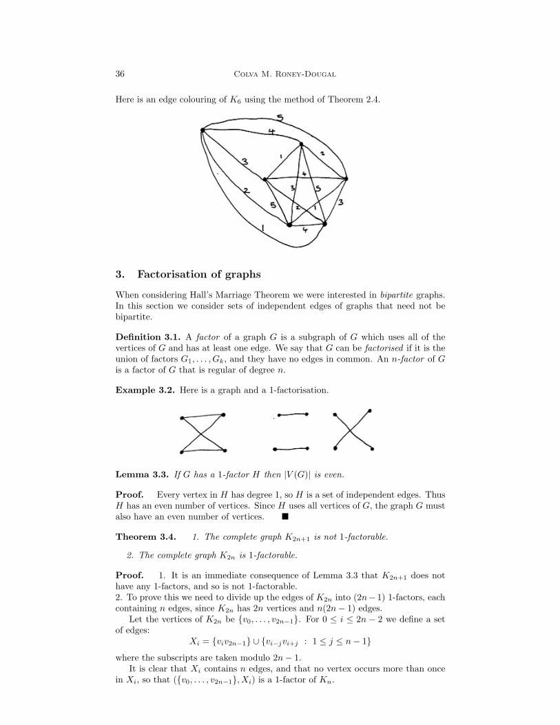
36 Colva M. Roney-Dougal
Here is an edge colouring of K6 using the method of Theorem 2.4.
3. Factorisation of graphs
When considering Hall’s Marriage Theorem we were interested in bipartite graphs.In this section we consider sets of independent edges of graphs that need not bebipartite.
Definition 3.1. A factor of a graph G is a subgraph of G which uses all of thevertices of G and has at least one edge. We say that G can be factorised if it is theunion of factors G1, . . . , Gk, and they have no edges in common. An n-factor of Gis a factor of G that is regular of degree n.
Example 3.2. Here is a graph and a 1-factorisation.
Lemma 3.3. If G has a 1-factor H then |V (G)| is even.
Proof. Every vertex in H has degree 1, so H is a set of independent edges. ThusH has an even number of vertices. Since H uses all vertices of G, the graph G mustalso have an even number of vertices. �
Theorem 3.4. 1. The complete graph K2n+1 is not 1-factorable.
2. The complete graph K2n is 1-factorable.
Proof. 1. It is an immediate consequence of Lemma 3.3 that K2n+1 does nothave any 1-factors, and so is not 1-factorable.2. To prove this we need to divide up the edges of K2n into (2n− 1) 1-factors, eachcontaining n edges, since K2n has 2n vertices and n(2n− 1) edges.
Let the vertices of K2n be {v0, . . . , v2n−1}. For 0 ≤ i ≤ 2n − 2 we define a setof edges:
Xi = {viv2n−1} ∪ {vi−jvi+j : 1 ≤ j ≤ n− 1}
where the subscripts are taken modulo 2n− 1.It is clear that Xi contains n edges, and that no vertex occurs more than once
in Xi, so that ({v0, . . . , v2n−1}, Xi) is a 1-factor of Kn.

Graph Theory 37
We check that no edge occurs in both Xi and Xk, for 0 ≤ i < k ≤ 2n − 2. Lete = vavb be an edge in both Xi and Xk. If a or b is 2n− 1 then the other vertex isvi in Xi and vk 6= vi in Xk, a contradiction. Thus we may assume without loss ofgenerality that a ≡ i− j mod (2n− 1) and b ≡ i + j mod (2n− 1) for some j, andthat {a, b} ≡ {k − l, k + l} mod (2n − 1) for some l. If i − j ≡ k − l mod (2n − 1)and i− j + 2j ≡ i + j ≡ k + l mod (2n− 1) then we deduce that j = l and so i = k,a contradiction. If i− j ≡ k + l mod (2n− 1) and i + j ≡ k − l mod (2n− 1) thenwe deduce that 2l ≡ 0 mod (2n− 1), also a contradiction.
Thus K2n can be 1-factorised as a sum of X0, X1, . . . , X2n−2. �
Example 3.5. Here is a 1-factorisation of K6 using the method of Theorem 3.4
By an odd component of a graph, we mean a connected component with an oddnumber of vertices. A proof of the following can be found in Harary, Theorem 9.4.
Theorem 3.6 (Tutte, 1947) A graph G has a 1-factor if and only if |V (G)| iseven and there is no set S of vertices such that the number of odd components ofG \ S is greater than |S|.
It can be awkward to use this theorem to prove that a 1-factor exists, as onemust consider all possible sets of vertices. However, the following example showsthat we can easily use it to show that a 1-factor does not exist.
Example 3.7. The following graph has an even number of vertices. If the setS = {v1, v2} is removed from G then four isolated vertices (and hence four oddcomponents) are left over, so G does not have a 1-factor.
What about 2-factorisations? If a graph is 2-factorable, then each factor mustbe a union of disjoint cycles, as these are the connected graphs that are regular ofdegree 2.
We have seen that the complete graph K2n is 1-factorable but that K2n+1 is not1-factorable.
Theorem 3.8. 1. The graph K2n is not 2-factorable.

38 Colva M. Roney-Dougal
2. The graph K2n+1 is 2-factorable.
Proof. 1. In K2n all vertices have odd degree, but all vertices of a 2-factorablegraph must have even degree.2. Label the vertices of K2n+1 as v0, v1, . . . , v2n. For 0 ≤ i ≤ n− 1 we construct apath Pi as follows:
Pi = vivi−1vi+1vi−2vi+2 · · · vi+n−1vi−n,
where the subscripts are taken modulo 2n. We then join v2n to the two endpointsof Pi to make a cycle, Zi.
We claim that Zi is a 2-factor, and that every edge lies in exactly one of theZi. It is clear that Pi contains 2n different vertices, none of which are v2n since thesubscripts are taken modulo 2n, therefore Zi is a 2-factor.
Let vavb be an edge in Zi and Zk, and assume (by way of contradiction) thati 6= k. If either of a or b is 2n then the other is either i or i− n in Zi, and either kor k−n in Zk. Since i 6= k we get k ≡ i−n mod 2n, a contradiction. Thus withoutloss of generality we may assume that for some j the pair (a, b) = (vi−j , vi+j)or (vi+j , vi−j−1) and simultaneously for some l the pair (a, b) = (vk−l, vk+l) or(vk+l, vk−l−1). If i − j ≡ k − l mod 2n and i + j ≡ k + l mod 2n, then i = k,a contradiction. If i − j ≡ k + l mod 2n and i + j ≡ k − l − 1 mod 2n, then2l ≡ 1 mod 2n, a contradiction. If i+j ≡ k− l mod 2n and i−j−1 ≡ k+ l mod 2n,then 2l + 2j ≡ 1 mod 2n, a contradiction. If i + j ≡ k + l mod 2n and i− j − 1 ≡k − l − 1 mod 2n, then i = k, a contradiction. Thus Zi and Zk have no edge incommon. �
Example 3.9. Here is a 2-factorisation of K5, using the techniques of Theorem 3.8.
4. Connectivity of graphs
We now discuss a theorem which implies Hall’s Marriage Theorem 1.4 and which hasvery far-reaching practical applications. It concerns the number of paths connectingtwo given vertices v and w in a graph G.
Definition 4.1. Let v and w be vertices of a graph. Several paths from v to w areedge disjoint if different paths have no edges in common. They are vertex disjointif they have no vertices other than v and w in common.
Example 4.2. Here are three edge-disjoint paths from A to Z:

Graph Theory 39
In general we will be interested in finding the maximum number of edge-disjointpaths between two vertices.
Definition 4.3. Let G be a connnected graph, and let v and w be distinct verticesof G. A disconnecting set of G is a set of edges whose removal breaks G into morethan one component. A vw-disconnecting set of G is a set S of edges of G withthe property that any path from v to w includes an edge of S: note that it mustbe a disconnecting set for G. A vw-separating set of G is a set S of vertices (notincluding v or w) such that any path from v to w includes at least one vertex in S.
Theorem 4.4 (Menger’s Theorem (Edge version)) Let v and w be distinctvertices of a connected graph G. The maximum number of edge-disjoint paths be-tween v and w is equal to the size of the smallest vw-disconnecting set.
Proof. The maximum number of edge-disjoint paths from v to w certainly cannotexceed the size of the smallest vw-disconnecting set, as every such path must use adistinct edge from each vw-disconnecting set.
We use induction on the number e of edges of the graph G to show that thesenumbers are equal. If e = 1 then v and w are the only vertices, since G is connected.There is therefore a single path between them, and a single edge in the only vw-disconnecting set.
So suppose that the result holds for all graphs with fewer than e edges, and letG be a graph with e edges and a vw-disconnecting set S of size k, where S is assmall as possible. We must show that the maximum number of edge-disjoint pathsfrom v to w is k. There are two cases to consider.Case 1: Suppose first that not all of the edges in S are incident to v and not allof them are incident to w. The removal from G of the edges in S results in twodisjoint subgraphs U and W containing v and w, respectively.
We now define two new graphs, G1 and G2. The graph G1 is obtained from G byshrinking down all of the vertices in U to a single vertex A, that is incident to allvertices that were incident to vertices of U in G: note that if there was more thanone edge from a vertex in U to a vertex in W then there will be a multiple edgefrom A to W in G1.
The graph G2 is obtained similarly, by shrinking all of the vertices in W downto a single vertex Z, which is incident to all vertices that were incident to verticesof W in G.

40 Colva M. Roney-Dougal
The graphs G1 and G2 have fewer edges than G, because there is at least one edgein U that is not in S, and at least one edge in W that is not in S. Since S is aminimal Aw-disconnecting set in G1 and vZ-disconnecting set in G2, the inductionhypothesis tells us that there are k edge-disjoint paths in G1 from A to w and inG2 from v to Z. The required k edge-disjoint paths in G are then obtained bycombining these paths in the obvious way.Case 2: Suppose that every vw-disconnecting set S of size k consists only of edgesthat are all incident to v or all incident to w. We can assume by induction thatevery edge of G is contained in one of these minimum vw-disconnecting sets, sinceotherwise its removal would not affect the value of k and we could use the inductionhypothesis to obtain k edge-disjoint paths. It follows that if P is any path fromv to w then P must consist of either one or two edges, and therefore contains atmost one edge of any vw-disconnecting set of size k. By removing all edges in Pfrom G, we obtain a graph which contains at least k− 1 edge-disjoint paths (by theinduction hypothesis). These (k − 1) paths, together with P , give the required kpaths in G. �
Theorem 4.5 (Menger’s theorem (vertex version)) Let v and w be distinctnonadjacent vertices of a graph G. The maximum number of vertex disjoint pathsfrom v to w is equal to the minimum number of vertices in a vw-separating set.
Exercise 4.6. The proof of the vertex version of Menger’s theorem is very similarto that of the edge version, try to write it down.
We finish by showing that Hall’s Marriage Theorem 1.4 can be deduced fromthe vertex version of Menger’s theorem.
Theorem 4.7. Theorem 4.5 implies Hall’s Marriage Theorem 1.4.
Proof. Let G be a connected bipartite graph with vertex sets V1 and V2. Wehave to show that it follows from Theorem 4.5 that if each set A ⊂ V1 of verticeshas at least |A| neighbours then there exists a matching from V1 to V2. Make a newgraph G1 by adjoining to G a vertex v that is adjacent to every vertex in V1 and avertex w that is adjacent to every vertex in V2.
Graph Theory 41
A matching from V1 to V2 exists if and only if the number of vertex-disjoint pathsfrom v to w is equal to the number of vertices in V1. Let |V1| = k. By Theorem 4.5,it is therefore enough to show that every vw-separating set contains at least kvertices.
Let S be a vw-separating set, consisting of a subset A of V1 and a subset Bof V2. Since S = A ∪ B is a vw-separating set, there are no edges joining verticesin V1 \ A to vertices in V2 \ B, otherwise there would be paths using these edgesbetween v and w. Therefore, the neighbours of V1 \ A that lie in V2 must all be inB. By assumption, the set V1 \A of vertices has at least |V1 \A| neighbours in V2.We deduce that
|V1 \A| ≤ |B|,
so |S| = |A|+ |B| ≥ |A|+ |V1 \A| = |V1| = k, as required. �

Chapter 6
Trees
1. Characterisation of Trees
In this section we study some properties of trees.
Definition 1.1. A graph with no circuits is a forest. Recall that a tree is a con-nected graph that contains no circuits.
In many ways a tree is the simplest type of graph. They have many nice proper-ties which often enable one to prove results about trees which are too hard to proveabout graphs in general.
There are many equivalent ways of defining trees, the following theorem collectssome of them.
Theorem 1.2. Let G be a graph with v vertices and e edges. The following areequivalent:
1. G is a tree;
2. G contains no circuits and e = v − 1;
3. G is connected and e = v − 1;
4. G is connected but the removal of any edge disconnects G;
5. Any two vertices of G are connected by exactly one path;
6. G contains no circuits, but the addition of any edge creates exactly one circuit.
Proof. If v = 1 then all of these results are trivial, so we assume throughoutthat v ≥ 2.
(1) ⇒ (2): By definition G contains no circuits. We prove by induction thate = v − 1. For v = 2 the only tree has 1 edge, so the result holds. Assume thatthe result is true for all trees with at most v − 1 edges. Let ab be an edge in G,and consider what happens when we remove ab. If there were still a path from ato b then there would originally have been more than one way of getting from ato b, so G would have contained a cycle. Therefore the removal of ab disconnectsG into two components, which are trees on v1 and v2 vertices, with v1 + v2 = v.Inductively these trees have v1 − 1 and v2 − 1 edges, so the total number of edgesin G is (v1 − 1) + (v2 − 1) + 1 = v − 1.
(2) ⇒ (3): Assume that the connected components of G are C1, . . . , Ck, onv1, . . . , vk vertices with v = v1 + v2 + · · ·+ vk. Since G contains no circuits, each Ci
is connected and contains no circuits, so is a tree. Therefore by (1) ⇒ (2) we havee =
∑ki=1(vi − 1) = v − k. Since e = v − 1 we have k = 1, so G is connected.
42

Graph Theory 43
(3) ⇒ (4): The removal of an edge from G produces a graph H with v−2 edges.We prove by induction that any graph with v − 2 edges is disconnected. If v = 2then the result is clear, so assume inductively that the result holds for all graphs onless than v vertices. The sum of the vertex degrees in H is 2(v − 2). If H has anyvertices of degree 0 then H is disconnected and we are done, so all vertices in H areincident to at least one edge. Since 2v > 2(v− 2) there exists at least one vertex, wsay, of H that has degree 1. Consider the graph H ′ produced by removing w andthe edge ending at w. This is a graph with v− 1 vertices and v− 3 edges, so by theinductive hypothesis H ′ is disconnected. Therefore H is disconnected.
(4) ⇒ (5): Since G is connected there exists at least one path from any vertex toany other. If two vertices were connected by more than one path, then it would bepossible to remove an edge from G, lying on one of the paths, without disconnectingG. Therefore any two vertices are connected by exactly one path.
(5) ⇒ (6): If G contained a circuit, then any pair of vertices on the circuit wouldbe connected by at least two chains. If an edge ab is added to G then a circuit willbe created, since there is already a path from a to b. If more than one circuit iscreated then there must be more than one path from a to b in G, a contradiction.
(6) ⇒ (1): If G is disconnected, then the addition of an edge between onecomponent of G and another would not create a circuit, a contradiction. ThereforeG is connected and contains no circuits, so is a tree. �
A vertex of degree 1 is called an endpoint.
Corollary 1.3. 1. Every nontrivial tree has at least two endpoints.
2. Let G be a forest with n vertices and k components, then G has n− k edges.
Exercise 1.4. Prove this corollary.
2. Counting Trees
We have already seen that people are interested in counting graphs. Whilst in gen-eral graph counting problems can be very hard, if we restrict ourselves to countingtrees then there are strong results. In this section we present a famous result byCayley in 1889 on the number of labelled trees.
Definition 2.1. A labelled graph is a pair (G, φ) where G is a graph on v verticesand φ is a bijection from the vertices of G to the set {1, . . . , v}. Less formally,we associate to each vertex of G a distinct number from {1, . . . , v}. Two labelledgraphs (G1, φ1) and (G2, φ2) are isomorphic if there is a graph isomorphism fromG1 to G2 that preserves the labelling of the vertices.
Example 2.2. The first of these graphs is labelled, the second is not.
The first two of these labelled graphs are isomorphic as labelled graphs. The thirdgraph is isomorphic as a graph to the first two, but not as a labelled graph sincethe vertex of degree 4 has a different label.

44 Colva M. Roney-Dougal
We now consider counting isomorphism classes of labelled graphs.
Example 2.3. This picture shows various ways of labelling a tree with four ver-tices:
The second tree is the reverse of the first one, and so is isomorphic to it. Neitherof them is isomorphic to the third tree, as it has a vertex of degree 2 and label 4.It follows that there are (4!)/2 = 12 ways of labelling this tree, since the reverse ofany labelling does not result in a new one.
Similarly, there are four ways of labelling this tree:
since the labelling is completely determined by the label of the middle vertex.Since these are the only trees on four vertices, there are 16 isomorphism classes
of labelled trees on four vertices.
We now consider the general case of labelled trees on n vertices. We will countthe labelled trees on n vertices by establishing a bijection between labelled treeswith n vertices and certain sequences of n− 2 numbers. We assume that n ≥ 3.
Definition 2.4. A Prufer sequence is a sequence of the form (a1, a2, . . . , an−2),where each ai ∈ {1, . . . , n} and repetitions are allowed.
Here is an algorithm which constructs a Prufer sequence from a labelled tree:
1. Look at the vertices of degree 1 and choose the one, w say, with the smallestlabel.
2. Find the vertex adjacent to w and place its label in the first available positionin the sequence.
3. Remove w and its incident edge, leaving a smaller tree.
4. Repeat steps 1 to 3 until there are only two vertices left, at which point asequence of length n− 2 will have been constructed.
Example 2.5. Consider the following labelled tree:

Graph Theory 45
1. The vertices of degree 1 are vertices 3, 5, 6 and 8, the one with the smallestlabel is vertex 3.
2. The vertex adjacent to vertex 3 is vertex 2, so the sequence starts with 2.
3. Removing vertex 3 and its incident edge gives the following tree:
4. The vertices of degree 1 are vertices 5, 6 and 8, the smallest label is vertex 5.
5. The vertex adjacent to vertex 5 is vertex 2, so the next number in the sequenceis 2.
6. Removing vertex 5 and its incident edge gives the following tree:
7. The vertices of degree 1 are vertices 2, 6 and 8, the smallest label is vertex 2.
8. The vertex adjacent to vertex 2 is vertex 4, so the next number in the sequenceis 4.
9. Removing vertex 2 and its incident edge gives the following tree:
10. Continue in the way, removing the edges (6, 1), (1, 4), (4, 7) to get the Prufersequence (2, 2, 4, 1, 4, 7).
In order to reverse the operation, we take a Prufer sequence and apply thefollowing three steps:
1. Draw the n vertices, labelling them from 1 to n, and make a list L of thenumbers from 1 to n.

46 Colva M. Roney-Dougal
2. Find the smallest number a that is in L but not in the Prufer sequence, andalso find the first number in the Prufer sequence. Draw an edge joining thevertices with these labels.
3. Remove the first number from L, and the first number from the Prufer se-quence, leaving a smaller list and sequence.
4. Repeat steps 2 and 3 for the remaining list and sequence until there are onlytwo numbers left in the list. Finish by joining the vertices with these labels.
Example 2.6. Consider the Prufer sequence (2, 2, 4, 1, 4, 7).
1. Since our Prufer sequence contains 8 − 2 = 6 numbers we start with the list[1, 2, 3, 4, 5, 6, 7, 8] and draw the vertices 1 to 8 as shown:
2. The smallest number in the list but not in the Prufer sequence is 3, and thefirst number in the Prufer sequence is 2, so we add an edge joining vertices 2and 3, as shown:
3. Our new list is [1, 2, 4, 5, 6, 7, 8] and our new sequence is (2, 4, 1, 4, 7).
4. The smallest number in the list but not the sequence is 5, and the first numberin the sequence is 2, so we add an edge joining vertices 2 and 5, as shown:
5. Our new list is [1, 2, 4, 6, 7, 8] and our new sequence is (4, 1, 4, 7).
6. The smallest number in the list but not in the sequence is 2, and the firstnumber in the sequence is 4, so we add an edge joining vertices 2 and 4, asshown:

Graph Theory 47
7. Our new list is [1, 4, 6, 7, 8] and our new sequence is (1, 4, 7).
8. The smallest number in the list but not in the sequence is 6, and the firstnumber in the sequence is 1, so we add an edge joining vertices 1 and 6, asshown:
9. Our new list is [1, 4, 7, 8] and our new sequence is (4, 7).
10. We then add an edge between vertices 1 and 4, then one between 4 and 7.Finally our list consists of the two numbers [7, 8], so we join the vertices withthese labels. This gives the following labelled tree:
Note that the labelled tree of this example is isomorphic to the tree of theprevious example. This is true in general: if you start with a tree, find the corre-sponding Prufer sequence, then construct a tree from the sequence, you get backan isomorphic labelled tree.
Theorem 2.7 (Cayley’s Theorem, 1889) There are nn−2 distinct labelled treeson n vertices.
Proof. We consider the above bijection between the set of labelled trees with nvertices and the set of all sequences of the form (a1, . . . , an−2) with ai ∈ {1, . . . , n}.There are exactly n possible values for each number ai, so the total number ofpossible sequences is nn−2, and the same holds for labelled trees. �

Chapter 7
Ramsey Theory
1. Graphs with no triangles
Given a graph, we can consider whether it contains triangles, quadrilaterals, tetra-hedra (triangle-based pyramids) like K4, or other geometric objects.
Example 1.1. The graph K3,3, or any other bipartite graph, contains no triangles,but K3,3 contains lots of quadrilaterals.
Question 1.2. How many edges can a simple graph on n vertices have withoutcontaining a triangle?
Answer: For n even, Kn/2,n/2 has n2/4 edges but no triangles. For n odd,K(n+1)/2,(n−1)/2 has (n2 − 1)/4 edges but no triangles. In fact, these bipartitegraphs give the most edges on n vertices with no triangles.
We prove this claim in the following theorem. Recall that bxc means the largestinteger less than or equal to x, known as the floor of x.
Theorem 1.3 (Turan’s Theorem) Let G be a simple graph on n vertices. If Gcontains no triangles then G has at most bn2/4c edges.
Proof. Let n = 2k be even. We prove the result for even n by induction on k:the proof for n odd is similar.
When k = 1 we have n = 2. The only simple graphs on 2 vertices are the graphwith 2 vertices and no edges and the graph with 2 vertices and one edge. Thesehave no triangles, and at most 22/4 = 1 edge, which starts the induction.
Assume inductively that the conclusion holds for graphs with at most n = 2kvertices. Let G have 2(k + 1) vertices and contain no triangle. Let vw be any edgeof G, and define G′ to be the graph obtained from G by removing the vertices vand w along with all edges ending at v or w.
The graph G′ has 2k vertices and contains no triangles, so by the inductivehypothesis G′ has at most bn2/4c = b(2k)2/4c = k2 edges. Now consider replacingthe removed edges and vertices to recover G. As G contains no triangles, v and wcannot both be joined to the same vertex z of G′ as this would give a triangle. Thenumber of edges we replace is therefore at most the number of vertices in G′, plusthe edge vw. Thus the number of edges in G is the number of edges of G′ plus thenumber of edges we replace, which is at most
k2 + 2k + 1 = (k + 1)2 = b(2(k + 1))2/4c
48

Graph Theory 49
This completes the inductive step, so the number of edges is at most k2 for all k.When n is odd the induction is similar, starting with the graph with one vertex,
no edges, and no triangles. �
Definition 1.4. The complement of a graph G has the same vertices as G, butwhenever G has an edge between two vertices the complement has a non-edgebetween those vertices, and whenever G has no edge between two vertices the com-plement has an edge.
We have seen that it is possible for a graph to have many edges and no triangles.However, in this situation the complement will have many triangles.
Example 1.5. Consider the following graph.
Here we have 6 vertices, 9 edges and no triangle. The complementary graph (withdashed edges) has two triangles.
Ramsey Theory. We proved in Chapter 1, Theorem 2.7 that in a group of sixpeople there are either three who mutually know each other or three who mutuallydon’t know each other. In the previous sentence, we can replace (6, 3) by (18, 4)and it will still be true. These are the prototype Ramsey Theorems. We representpeople by vertices of a complete graph, and colour the edge vw red if v and w knoweach other, and blue otherwise.
Note that we are now talking about colouring the edges of a graph, rather thanthe vertices as in Chapter 4.
Proposition 1.6. If the edges of K18 are all coloured either red or blue, then thereis either a red K4 or a blue K4.
This proposition will follow from a more general result given in the next section.
2. Ramsey Numbers
Definition 2.1. By the Ramsey number R(m,n) we denote the least integer suchthat when the edges of the complete graph KR(m,n) are all coloured either red orblue then the graph contains either a red Km or a blue Kn.
For example, we have seen that R(3, 3) = 6 and claimed that R(4, 4) = 18.
Proposition 2.2. For all m ≥ 2 and n ≥ 2 we have
R(m,n) ≤ R(m,n− 1) + R(m− 1, n).
In particular, R(m,n) is always finite.

50 Colva M. Roney-Dougal
Proof. Consider a complete graph with R(m,n− 1) + R(m− 1, n) vertices, andall edges coloured either red or blue. Each vertex has degree R(m,n− 1) + R(m−1, n)− 1. So for any vertex v, either at least R(m,n− 1) of the edges incident to vare blue or at least R(m− 1, n) of them are red.
Assume first that at least R(m,n−1) of the edges are blue, joining v to verticesv1, v2, . . . , vR(m,n−1) (and possibly some other vertices too). Consider the edgesjoining these vi to one another. They form KR(m,n−1) and so either these verticescontain a red Km, in which case we are done, or they form a blue Kn−1. In thissecond case v and all of the edges that are joined in this Kn−1 form a blue Kn.
By a similar argument, if at least R(m−1, n) of the edges at v are red, we againget either a red Km containing v, or a blue Kn amongst the vertices that are joinedto v by red edges. �
Corollary 2.3. We have
R(m,n) ≤ (m + n− 2)!(m− 1)!(n− 1)!
=(
m + n− 2m− 1
).
Proof. We prove this by double induction using Proposition 2.2. The graph K1
(a single isolated vertex) always contains K1, so we have R(m, 1) = R(1, n) = 1.Therefore
1 = R(m, 1) ≤ (m + 1− 2)!(m− 1)!0!
=(m− 1)!(m− 1)!
= 1.
A similar calculation shows that R(1, n) also satisfies the inequality, so the corollaryis true when either m or n is 1.
The graph Km either contains a red Km or has at least one blue edge, giving ablue K2, so R(m, 2) = m, and similarly R(2, n) = n. Therefore
m = R(m, 2) ≤ (m + 2− 2)!(m− 1)!1!
=m!
(m− 1)!= m,
and similarly for R(2, n). These cases found the induction.Assume inductively the corollary holds for R(i, j) with i ≤ m − 1 and j ≤ n,
and for R(i, j) with i ≤ m and j ≤ n− 1. By Proposition 2.2 we have
R(m,n) ≤ R(m,n− 1) + R(m− 1, n)≤ (m+n−3)!
(m−1)!(n−2)! + (m+n−3)!(m−2)!(n−1)! by the inductive hypothesis
= (m+n−3)!(m−1)!(n−1)! ((n− 1) + (m− 1))
= (m+n−2)!(m−1)!(n−1)!
The result therefore holds for R(m,n) and so for all m and n by induction. �
Remark 2.4. Proposition 2.2 does not always give best results. For example,
9 = R(3, 4) < R(3, 3) + R(2, 4) = 6 + 4 = 10.
Theorem 2.5. The following are values for R(m,n):
R(m,n) m1 2 3 4 5 6 7 8 9 10 . . .
1 1 1 1 1 1 1 1 1 1 1 . . .2 1 2 3 4 5 6 7 8 9 10 . . .3 1 3 6 9 14 18 23 28 36 40–43
n 4 1 4 9 18 25 35–41 49–61 56–845 1 5 14 25 43–496 1 6 18...
...

Graph Theory 51
Challenges Find R(3, 10), R(3, 11), R(4, 6), R(5, 5), . . ..
3. Ramsey numbers for several colours
We write Rk(3) = R(3, 3, . . . , 3) (with k threes) for the smallest number such thatif the edges of the complete graph on Rk(3) vertices are coloured with k coloursthen we can find a monochromatic triangle.
For example, R2(3) = R(3, 3) = 6. We have Rk(3) ≤ (k + 1)!.
Theorem 3.1 (An application to number theory) Let m = Rk(3)− 1. If theintegers 1, 2, . . . ,m are coloured with k colours then the equation x + y = z has asolution with x, y and z all the same colour.
For example, suppose k = 2 and m = 5 (recall that R2(3) = 6), and that wecolour 1 and 3 black and 2, 4 and 5 red. Then 2 + 2 = 4 is a red solution.
Proof. Fix a colouring of the numbers 1, . . . ,m. Label the vertices of KRk(3)
with the integers 1, 2, . . . ,m, m+1 and colour the edge rs the colour of the number|r − s|. Then by definition of Rk(3) we may find a monochromatic triangle in thisgraph, with vertices a, b, c such that
1 ≤ a < b < c ≤ m + 1.
Let x = b− a, y = c− b and z = c− a. Then the numbers x, y, z represent edges inthe triangle, so they all have the same colour. Also,
x + y = (b− a) + (c− b) = c− a = z.
�
Remark 3.2. This theorem also holds for all m ≥ Rk(3)− 1.
Next we consider infinite graphs.
Theorem 3.3 (Ramsey’s Theorem) Let V be a countably infinite set of verticeswith each distinct pair joined by a red or blue edge. Then V has an infinite subsetof vertices {a0, a1, . . .} joined by edges all of the same colour.
Proof. We divide the proof into two casesCase (i): There is an infinite subset A of V such that just finitely many vertices ofA are red-joined to infinitely many other vertices of A.
Delete the vertices of A which have infinite red degree to get an infinite set A′
with all vertices red-joined to only finitely many other vertices of A. We now selectinductively a sequence of vertices ak all blue joined.
Take a0 ∈ A′. Suppose we have selected a0, a1, . . . , ak ∈ A′ all blue joined. Sincethese vertices are joined to only finitely many points of A′ by red edges they arejoined to an infinite number of points of A′ by only blue edges. Therefore we maypick a new point ak+1 ∈ A′ that is blue joined to all of a0, a1, . . . , ak. Continuingin this way we get an infinite sequence of vertices a0, a1, . . . all blue joined.Case (ii): Every infinite subset A of V contains infinitely many vertices red-joinedto infinitely many other vertices of A.
In this case we select inductively a sequence of vertices ak that are all red-joined.Take a0 ∈ V with infinite red degree and let A0 be the infinite set of vertices redjoined to a0. Suppose inductively that there are points a0, a1, . . . , ak all red-joinedand an infinite set of vertices Ak all red-joined to all of a0, a1, . . . , ak. Take a newpoint ak+1 ∈ Ak that is red-joined to infinitely many other vertices of Ak (since
52 Colva M. Roney-Dougal
we are in case (ii)), and let Ak+1 be the infinite subset of Ak of points red joinedto ak+1. Then a0, a1, . . . , ak+1 are all red-joined to each other and to all points ofAk+1. Proceeding in this way gives an infinite sequence of vertices a0, a1, . . . allred-joined. �
Corollary 3.4. Let V be an infinite set of vertices with each pair joined by an edgecoloured by one of k colours. Then V has an infinite subset of vertices {a0, a1, . . .}joined by edges all of the same colour.
Proof. Let the colours be c1, c2, . . . , ck. By Ramsey’s Theorem 3.3, there iseither an infinite set of vertices with all joining edges coloured c1 or an infinite setwith joining edges coloured only by colours c2, . . . , ck. In the latter case, continue toapply Ramsey’s Theorem up to (k− 1) more times until an infinite set with joiningedges of one colour is reached. �
Corollary 3.5. There is an infinite subset S of N such that for all distinct m,n ∈ Sthe number m + n has an even number of prime factors (including multiplicity).
Proof. Consider a graph with vertices the natural numbers. Join m to n by ared edge if m + n has an even number of prime factors. Join m to n by a blue edgeif m + n has an odd number of prime factors. By Ramsey’s theorem either there isan infinite subset of integers all red-joined, in which case the result follows, or thereis an infinite subset T = {a1, a2, . . .} that are all blue-joined. In this case ai + aj
always has an odd number of prime factors, so the set S = {2a1, 2a2, 2a3, . . .} givesthe result. �
Consider a set S with |S| = 3, say S = {3, 7, 18}. Here 3 + 7 = 10 = 2 · 5,3 + 18 = 21 = 3 · 7, 7 + 18 = 25 = 52, so all sums have an even number of factors.Challenge Find a specific infinite set S with the property in the corollary.
Corollary 3.6. Let a1, a2, . . . be an infinite sequence of real numbers. Then thissequence either has an infinite increasing subsequence a′1 ≤ a′2 ≤ . . . or a decreasingsubsequence a′1 ≥ a′2 ≥ . . ..
Proof. Consider a graph whose vertices are the natural numbers. If i > j thenwe red-join i to j if ai ≥ aj and blue-join i to j if ai < aj . By Ramsey’s theoremthere is an infinite subset a′1, a
′2, . . . (in that order) such that either all corresponding
integers are red-joined, in which case a′i ≥ a′j whenever i > j so the sequence isincreasing, or they are all blue-joined in which case a′i < a′j whenever i > j so thesequence is decreasing. �

Chapter 8
Adjacency matrices
Aim: To use results from Linear Algebra to study the structure of graphs.
1. Definitions and basic results
Definition 1.1. Let G be a simple (undirected) graph with v vertices p1, . . . , pv.The adjacency matrix A of G is the v × v square matrix such that
aij = [A]ij ={
1 if pipj is an edge0 otherwise
Thus A records which pairs of vertices are joined by an edge.
Example 1.2. Consider the following graph:
The corresponding adjacency matrix is:
A =
0 1 0 11 0 1 10 1 0 11 1 1 0
We collect some straightforward facts in the following lemma.
Lemma 1.3. Let A be the adjacency matrix of a simple graph with vertices p1, . . . , pv.
1. A is a symmetric matrix with 0s on the diagonal and 0 or 1 elsewhere.
2. For each i, the sum of the entries in the ith row,∑v
j=1 aij, equals the degreeof pi.
3. A2 has (i, j) entry∑v
k=1 aikakj. This sum counts 1 for every vertex pk thatis joined to both pi and pj. This is the number of different paths of length twofrom pi to pj. In particular the diagonal entries of A2 are the degrees of thevertices.
4. Am gives the number of paths of length m between vertices pi and pj, wherewe allow paths to traverse edges several times.
53

54 Colva M. Roney-Dougal
Remark 1.4. We may define adjacency matrices in the same way for non-simplegraphs, with aij = x if pi and pj are joined by x edges, and for directed graphs (inwhich case A is not necessarily symmetric).
Example 1.5. In Example 1.2 we have
A2 =
2 1 2 11 3 1 22 1 2 11 2 1 3
Since [A2]1,3 = 2 there are two paths of length two from p1 to p3 (via p2 or p4).Similarly,
A3 =
2 5 2 55 4 5 52 5 2 55 5 5 4
.
Note that the sum of the diagonal entries gives the number of triangles in the graph,with each triangle counted six times. So the number of triangles in the graph ofExample 1.2 is (2 + 4 + 2 + 4)/6 = 2.
2. Eigenvalues
Recall that λ is an eigenvalue of a square matrix A if
det(A− λI) = 0
and that this holds if and only if there exists a vector x 6= 0 such that
Ax = λx.
Such an x is called an eigenvector.Note that a v × v real matrix A has v real or complex eigenvalues, which are
not necessarily all distinct, since det(A− λI) is a polynomial of degree v in λ.
Lemma 2.1. Let A be a square real matrix and suppose that A satisfies a polyno-mial equation. Then every eigenvalue of A satisfies the same polynomial equation.
Proof. Suppose bnAn + bn−1An−1 + · · ·+ b1A+ b0I = 0. Let λ be any eigenvalue
of A. Then Ax = λx for some vector x 6= 0. Therefore, A2x = λAx = λ2x, andsimilarly Akx = λkx for 2 ≤ k ≤ n. Therefore
0 = 0x= (bnAn + · · ·+ b1A + b0I)x= (bnλn + · · ·+ b1λ + b0)x
Since bnλn + · · ·+ b1λ + b0 is a real or complex number and x is a nonzero vector,this implies that bnλn + · · ·+ b1λ + b0 = 0. �
Recall that the trace of a square matrix is the sum of its diagonal entries.
Lemma 2.2. For any v × v matrix A, the sum of the eigenvalues of A (countedwith multiplicities) is equal to the trace of A.
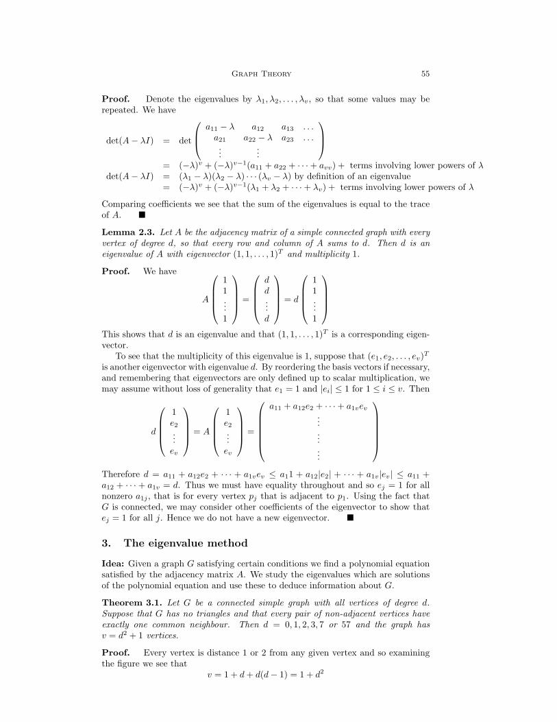
Graph Theory 55
Proof. Denote the eigenvalues by λ1, λ2, . . . , λv, so that some values may berepeated. We have
det(A− λI) = det
a11 − λ a12 a13 . . .a21 a22 − λ a23 . . ....
...
= (−λ)v + (−λ)v−1(a11 + a22 + · · ·+ avv) + terms involving lower powers of λ
det(A− λI) = (λ1 − λ)(λ2 − λ) · · · (λv − λ) by definition of an eigenvalue= (−λ)v + (−λ)v−1(λ1 + λ2 + · · ·+ λv) + terms involving lower powers of λ
Comparing coefficients we see that the sum of the eigenvalues is equal to the traceof A. �
Lemma 2.3. Let A be the adjacency matrix of a simple connected graph with everyvertex of degree d, so that every row and column of A sums to d. Then d is aneigenvalue of A with eigenvector (1, 1, . . . , 1)T and multiplicity 1.
Proof. We have
A
11...1
=
dd...d
= d
11...1
This shows that d is an eigenvalue and that (1, 1, . . . , 1)T is a corresponding eigen-vector.
To see that the multiplicity of this eigenvalue is 1, suppose that (e1, e2, . . . , ev)T
is another eigenvector with eigenvalue d. By reordering the basis vectors if necessary,and remembering that eigenvectors are only defined up to scalar multiplication, wemay assume without loss of generality that e1 = 1 and |ei| ≤ 1 for 1 ≤ i ≤ v. Then
d
1e2
...ev
= A
1e2
...ev
=
a11 + a12e2 + · · ·+ a1vev
...
...
...
Therefore d = a11 + a12e2 + · · · + a1vev ≤ a11 + a12|e2| + · · · + a1v|ev| ≤ a11 +a12 + · · · + a1v = d. Thus we must have equality throughout and so ej = 1 for allnonzero a1j , that is for every vertex pj that is adjacent to p1. Using the fact thatG is connected, we may consider other coefficients of the eigenvector to show thatej = 1 for all j. Hence we do not have a new eigenvector. �
3. The eigenvalue method
Idea: Given a graph G satisfying certain conditions we find a polynomial equationsatisfied by the adjacency matrix A. We study the eigenvalues which are solutionsof the polynomial equation and use these to deduce information about G.
Theorem 3.1. Let G be a connected simple graph with all vertices of degree d.Suppose that G has no triangles and that every pair of non-adjacent vertices haveexactly one common neighbour. Then d = 0, 1, 2, 3, 7 or 57 and the graph hasv = d2 + 1 vertices.
Proof. Every vertex is distance 1 or 2 from any given vertex and so examiningthe figure we see that
v = 1 + d + d(d− 1) = 1 + d2
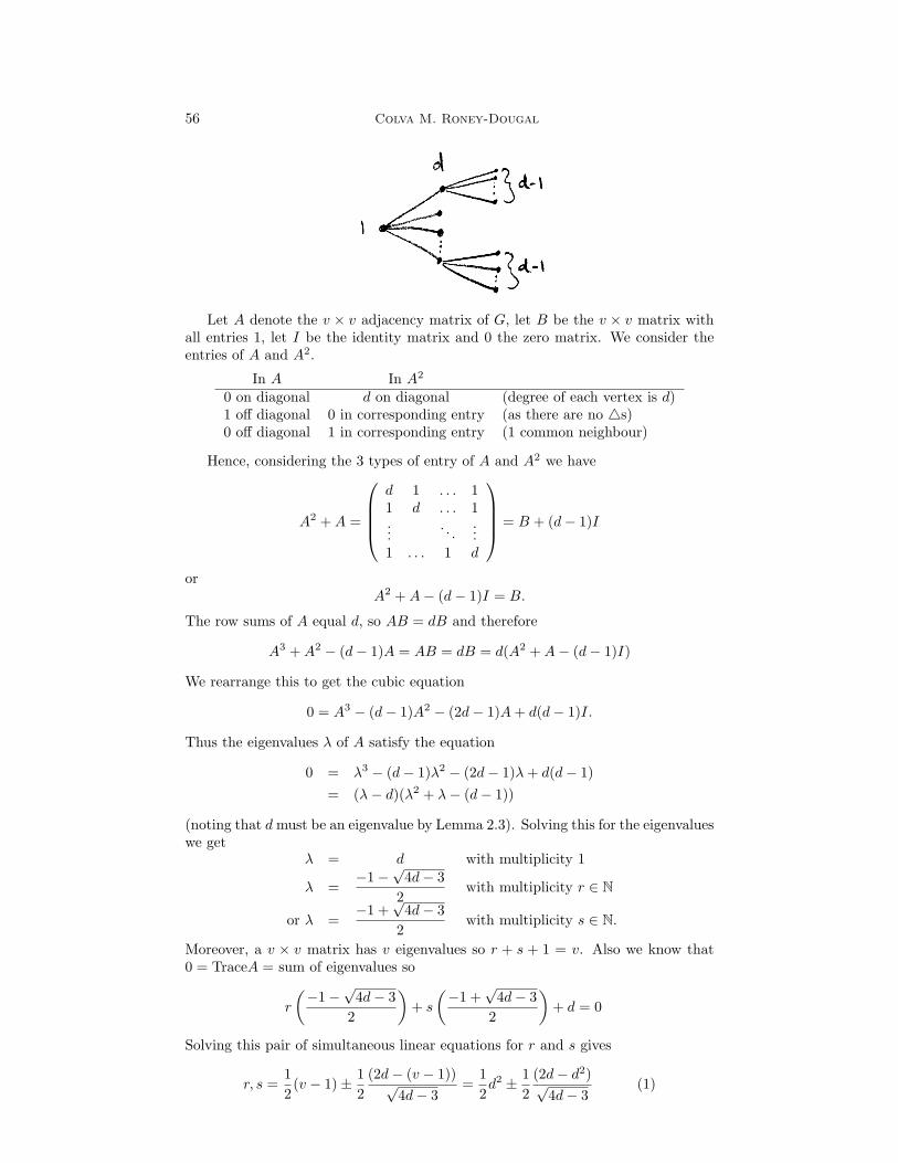
56 Colva M. Roney-Dougal
Let A denote the v × v adjacency matrix of G, let B be the v × v matrix withall entries 1, let I be the identity matrix and 0 the zero matrix. We consider theentries of A and A2.
In A In A2
0 on diagonal d on diagonal (degree of each vertex is d)1 off diagonal 0 in corresponding entry (as there are no 4s)0 off diagonal 1 in corresponding entry (1 common neighbour)
Hence, considering the 3 types of entry of A and A2 we have
A2 + A =
d 1 . . . 11 d . . . 1...
. . ....
1 . . . 1 d
= B + (d− 1)I
orA2 + A− (d− 1)I = B.
The row sums of A equal d, so AB = dB and therefore
A3 + A2 − (d− 1)A = AB = dB = d(A2 + A− (d− 1)I)
We rearrange this to get the cubic equation
0 = A3 − (d− 1)A2 − (2d− 1)A + d(d− 1)I.
Thus the eigenvalues λ of A satisfy the equation
0 = λ3 − (d− 1)λ2 − (2d− 1)λ + d(d− 1)= (λ− d)(λ2 + λ− (d− 1))
(noting that d must be an eigenvalue by Lemma 2.3). Solving this for the eigenvalueswe get
λ = d with multiplicity 1
λ =−1−
√4d− 3
2with multiplicity r ∈ N
or λ =−1 +
√4d− 3
2with multiplicity s ∈ N.
Moreover, a v × v matrix has v eigenvalues so r + s + 1 = v. Also we know that0 = TraceA = sum of eigenvalues so
r
(−1−
√4d− 3
2
)+ s
(−1 +
√4d− 3
2
)+ d = 0
Solving this pair of simultaneous linear equations for r and s gives
r, s =12(v − 1)± 1
2(2d− (v − 1))√
4d− 3=
12d2 ± 1
2(2d− d2)√
4d− 3(1)

Graph Theory 57
since v = 1 + d2.But r and s are integers, so from (1) either (i) (2d− d2) = 0 or (ii) 4d− 3 is a
perfect square (otherwise√
4d− 3, and thus r and s, would be irrational).In case (i), d = 0 (trivial) or d = 2 and v = 5 (giving a pentagon).In case (ii), setting t =
√4d− 3 for some integer t, we get d = 1
4 (t2 +3), so from(1)
s =12
[d2 +
(2d− d2)t
]=
12
[116
(t2 + 3)2 +2× 1
4 (t2 + 3)− 116 (t2 + 3)2
t
],
simplifying tot5 − t4 + 6t3 + 2t2 + (9− 32s)t + 15 = 0.
Thus t divides 15 (the product of the roots of this equation), so ±t = 1, 3, 5 or 15,giving d = 1
4 (t2 + 3) = 1, 3, 7 or 57. �
Now we prove a second, similar result.
Theorem 3.2. Let G be a connected simple graph. Suppose that every edge of Gbelongs to exactly one triangle, and every two non-adjacent vertices have exactly twocommon neighbours (i.e. form the (missing) diagonal of exactly one quadrilateral).Then every vertex has the same degree d, where d = 0, 2, 4, 14, 22, 112 or 974, withthe number of vertices v = 1 + 1
2d2.
Proof. Let v0 be some vertex of G. Then v0 must be the common vertex of nedge-disjoint triangles, T1, . . . , Tn, for some integer n.
Moreover, every pair of vertices (other than v0) from different triangles Ti has onefurther common neighbour. This accounts for all the vertices, as no vertices aredistance more than 2 apart. Counting these vertices
v = 1 + 2n +122n(2n− 2) = 1 + 2n2.

58 Colva M. Roney-Dougal
In particular (since we can count the vertices in this way starting with any vertexv0) every vertex has degree d = 2n for the same integer n.
Let A denote the v × v adjacency matrix of G, let B be the v × v matrix withall entries 1, let I be the identity matrix and 0 be the zero matrix. We collect somefacts about A and A2.
In A In A2
0 on diagonal 2n on diagonal (degree of each vertex is 2n)1 off diagonal 1 in corresponding entry (every edge belongs to 1 4)0 off diagonal 2 in corresponding entry (every non-edge is diagonal of 1 quadrilateral)
Hence, considering the 3 types of entry of A and A2, we have
A2 + A = 2B + (2n− 2)I
orA2 + A− (2n− 2)I = 2B.
We note that AB = 2nB since the row sums of A equal 2n, so
A3 + A2 − (2n− 2)A = 2AB = 4nB = 2n(A2 + A− (2n− 2)I).
Rearranging, we get the cubic
0 = A3 + (1− 2n)A2 + (2− 4n)A + 4n(n− 1)I.
Thus the eigenvalues λ of A satisfy the equation
0 = λ3 + (1− 2n)λ2 + (2− 4n)λ + 4n(n− 1)= (λ− 2n)(λ2 + λ− 2(n− 1))
(noting that d = 2n must be an eigenvalue, so that we can factorise out (λ− 2n)).Solving we find eigenvalues
λ = 2n with multiplicity 1
λ =−1−
√8n− 7
2with multiplicity r ∈ N
or λ =−1 +
√8n− 7
2with multiplicity s ∈ N.
Moreover, a v × v matrix has v eigenvalues so r + s + 1 = v = 1 + 2n2. Also0 =TraceA = sum of eigenvalues so
r
(−1−
√8n− 7
2
)+ s
(−1 +
√8n− 7
2
)+ 2n = 0.
Solving this pair of simultaneous linear equations for r and s gives
r, s = n2 ± (n2 − 2n)√8n− 7
.
But r and s are integers, so either (i) n(n − 2) = 0 or (ii)√
8n− 7 is an integerthat divides n(n − 2) (since the square root of an integer is either an integer or isirrational).
In case (i), n = 0 (trivial) or n = 2 and v = 9.In case (ii), set t =
√8n− 7 for some integer t so 8n = t2+7, and let n(n−2) = kt
for some integer k. Then8n(8n− 16) = 64kt,

Graph Theory 59
so(t2 + 7)(t2 − 9) = 64kt,
that ist4 − 2t2 − 64kt− 63 = 0.
Thus t divides 63 (the product of the roots of this equation), so we have the followingpossibilities:
t =√
8n− 7 : 1 3 7 9 21 63n = (t2 + 7)/8 : 1 2 7 11 56 487
d = 2n : 2 4 14 22 112 974v = 1 + 2n2 : 3 9 99 243 6273 494019
Graphs of this form with d = 2, 4, 22 are known to exist. �
Theorem 3.3. Let G be a connected simple graph with v vertices. Suppose that Gcontains no triangles, but that every pair of non-adjacent vertices have two commonneighbours. Then every vertex has the same degree d = n2 + 1 for some n ∈ N,where n is not a multiple of 4, and v = (n4 + 3n2 + 4)/2.
Proof. See tutorial sheet. �


![Jevgenia Viktorova University of St Andrews E-mail: jv2 [ät] st-and.ac.uk.](https://static.fdocuments.in/doc/165x107/551b46a3550346ae7a8b4d14/jevgenia-viktorova-university-of-st-andrews-e-mail-jv2-aet-st-andacuk.jpg)