MT3D-USGS Version 1: A U.S. Geological Survey … · Evapoconcentration Dissolution Crop ET...
84
Reduction/ Precipitation Soil matrix Sorption Desorption Mass removal Runoff concentration Applied concentration Unsaturated-zone transport Saturated-zone transport Bedrock Streamflow transport Evapoconcentration Dissolution Crop ET Riparian ET Crop ET Return flow loading/ Seepage loading Saturated-zone transport Bedrock Bedrock U.S. Department of the Interior U.S. Geological Survey Techniques and Methods 6-A53 A product of the Groundwater Resources Program Prepared in collaboration with S.S. Papadopulos & Associates, Inc. MT3D-USGS Version 1: A U.S. Geological Survey Release of MT3DMS Updated with New and Expanded Transport Capabilities for Use with MODFLOW
Transcript of MT3D-USGS Version 1: A U.S. Geological Survey … · Evapoconcentration Dissolution Crop ET...

Reduction/Precipitation
Soilmatrix
Sorption
Desorption
Massremoval
Runoffconcentration
Appliedconcentration
Unsaturated-zonetransport
Saturated-zonetransport
Bedrock
Streamflowtransport
Evapoconcentration
Dissolution
Crop ET
RiparianET
Crop ET
Return flow loading/Seepage loading
Saturated-zonetransport
BedrockBedrock
U.S. Department of the InteriorU.S. Geological Survey
Techniques and Methods 6-A53
A product of the Groundwater Resources Program
Prepared in collaboration with S.S. Papadopulos & Associates, Inc.
MT3D-USGS Version 1: A U.S. Geological Survey Release of MT3DMS Updated with New and Expanded Transport Capabilities for Use with MODFLOW

Cover. Conceptualization of salt movement between the Fort Lyon irrigation canal and Arkansas River located in southeastern Colorado. Non-point source pollutant feedback between surface water irrigation systems and alluvial aquifers require sophisticated groundwater solute transport codes. Photograph by Bill Cotton, Colorado State University.

MT3D-USGS Version 1: A U.S. Geological Survey Release of MT3DMS Updated with New and Expanded Transport Capabilities for Use with MODFLOW
By Vivek Bedekar, Eric D. Morway, Christian D. Langevin, Matt Tonkin
Groundwater Resources Program
Prepared in collaboration with S.S. Papadopulos & Associates, Inc.
Techniques and Methods 6-A53
U.S. Department of the InteriorU.S. Geological Survey

U.S. Department of the InteriorSALLY JEWELL, Secretary
U.S. Geological SurveySuzette M. Kimball, Director
U.S. Geological Survey, Reston, Virginia: 2016
For more information on the USGS—the Federal source for science about the Earth, its natural and living resources, natural hazards, and the environment—visit http://www.usgs.gov or call 1–888–ASK–USGS.
For an overview of USGS information products, including maps, imagery, and publications, visit http://www.usgs.gov/pubprod/.
Any use of trade, firm, or product names is for descriptive purposes only and does not imply endorsement by the U.S. Government.
Although this information product, for the most part, is in the public domain, it also may contain copyrighted materials as noted in the text. Permission to reproduce copyrighted items must be secured from the copyright owner.
Suggested citation:Bedekar, Vivek, Morway, E.D., Langevin, C.D., and Tonkin, Matt, 2016, MT3D-USGS version 1: A U.S. Geological Survey release of MT3DMS updated with new and expanded transport capabilities for use with MODFLOW: U.S. Geological Survey Techniques and Methods 6-A53, 69 p., http://dx.doi.org/10.3133/tm6A53.
ISSN 2328-7055 (online)

iii
PrefaceThis report describes an updated version of the MT3DMS computer program, hereafter
referred to as “MT3D-USGS.” MT3D-USGS can be used with many of the new features recently developed for MODFLOW. The overarching goals for developing MT3D-USGS are two fold—to keep pace with advancements in MODFLOW and to provide users of the MT3DMS solute transport simulator with expanded functionality for tackling increasingly complex water-quality issues.
MT3D-USGS has been tested with applications distributed with MT3DMS (obtained from http://hydro.geo.ua.edu/mt3d/), as well as with new applications described herein. As the num-ber of MODFLOW packages has grown, so too has the possibility for various inter-package flow exchanges (for example, water discharging to land surface can be amended to streamflow). Benchmark simulations have been designed to ensure that flow exchanges and associated solute transport work properly. However, as MT3D-USGS is applied to transport problems, previously undetected errors may be identified. In such instances, users are requested to send notifications of suspected errors either in this documentation or the model it describes to the contact listed on the MT3D-USGS webpage. Users are encouraged to check for model updates on the MT3D-USGS webpage (http://dx.doi.org/10.5066/F75T3HKD).
MT3D-USGS is not a replacement for MT3DMS. Separate updates to both codes will likely continue in the future. Therefore, MT3D users should check appropriate webpages for updates and releases of MT3D-USGS and MT3DMS separately.
AcknowledgmentsThe U.S. Geological Survey (USGS) Groundwater Resources Program provided financial
support for much of the work documented herein. We wish to thank Daniel Feinstein of the Wisconsin Water Science Center, Dave Berger of the Nevada Water Science Center, and Gary Curtis of the National Research Program for their thoughtful and constructive reviews of this report. We are especially grateful to Rich Niswonger of the Nevada Water Science Center for supporting and implementing the Link-Mass Transport (LMT) modifications in MODFLOW-NWT and for providing feedback during code development. We also wish to thank George Zyvoloski of the Los Alamos National Laboratory for graciously providing previously pub-lished datasets for the testing of MT3D-USGS.
Some transport capabilities documented in this report were developed to support the applica-tion of MT3D at the U.S. Department of Energy (DOE) Hanford Site under contract to CH2M Hill Plateau Remediation Company (CHPRC); and on behalf of the Zone 7 Water Agency, California. The kinetic reaction capability was developed under a contract to the U.S. Environ-mental Protection Agency (EPA), led by Dr. Jim Weaver.
MT3D, in all of its variations, would not exist without Professor Chunmiao Zheng. MT3D was first developed by Professor Zheng in 1990 while working at S.S. Papadopulos & Asso-ciates, Inc. (SSP&A) with partial support from the U.S. Environmental Protection Agency (USEPA). From the outset, MT3D was released as a pubic domain code, although commercial versions with enhanced capabilities were also developed. MT3DMS—the second generation of MT3D—was developed by Professor Zheng with funding from the U.S. Army Corps of Engineers Waterways Experiment Station under the Strategic Environmental Research and Development Program (SERDP) to possess expanded capabilities including, most critically, a multi-component program structure that accommodated “add-on” packages. Today, MT3DMS is an industry standard, accepted by practitioners and researchers and applied in thousands of studies worldwide. Its multi-component modular design and open-source availability facilitated the development of additional solute transport simulators used around the globe today. The development of MT3D-USGS documented in this report builds upon the continuing vision of Professor Zheng and the contributions and financial support of his many public and private-sector collaborators worldwide.

iv
Contents
Abstract ......................................................................................................................................................... 1Introduction ................................................................................................................................................... 1Mathematical Model and Formulations in MT3D-USGS ....................................................................... 6
Mathematical Model .......................................................................................................................... 6Numerical Formulation ....................................................................................................................... 6Storage Formulation for Saturated Conditions ............................................................................... 7Storage Formulation for Unsaturated Conditions ........................................................................ 10
Modifications to the Existing MT3DMS Program and Packages ...................................................... 12Memory Management ...................................................................................................................... 12Handling of Dry Cells ........................................................................................................................ 12
Original MT3DMS Solution ..................................................................................................... 13Use of the DRYCELL Option ..................................................................................................... 13
Dispersion (DSP) Package ............................................................................................................... 15Source-Sink Mixing (SSM) Package .............................................................................................. 15Reaction (RCT) Package ................................................................................................................... 16
Instantaneous Inter-Species Reactions ............................................................................... 16Monod Kinetics ......................................................................................................................... 16First-Order Parent-Daughter Chain Reactions .................................................................... 17Kinetic Reaction Between Multiple Electron Donors and Acceptors ............................. 17
Multi-Component Reactive Transport in Groundwater ............................................. 18Stoichiometry of Gasoline Component Biodegradation by Multiple
Electron Acceptors ................................................................................... 18Mass Transport Equations .................................................................................... 19Reaction Rates for the Electron Donors ED1 and ED2 ..................................... 20Reaction Rates for ED Utilization by Sequential EAs ........................................ 20Generalized Form of Equations Relating ED Degradation and EA
Consumption .............................................................................................. 22Additional Considerations ..................................................................................... 23
Implementation of Multi-Component Reactive Transport in MT3D-USGS ............. 24Program Structure and Solution of Equations ........................................................... 24
Separate Specification of Solid and Aqueous Phase Partitioning Coefficient in Mobile and Immobile Domains ................................................................................ 24
Hydrocarbon Spill Source (HSS) Package .................................................................................... 25HSS Package Summary ........................................................................................................... 25Finite-Difference Equations .................................................................................................... 25Implementation in MT3D-USGS ............................................................................................. 26Simulation Input Requirements and Instructions ................................................................ 26
New Transport Packages Developed for MT3D-USGS ........................................................................ 26Contaminant Treatment System (CTS) Package .......................................................................... 26
Implementation in MT3D-USGS ............................................................................................. 29Simulation Input Requirements and Instructions ................................................................ 29
Solute Transport Through Generalized Networks ....................................................................... 29Streamflow Transport (SFT) Package .................................................................................... 29

v
Implementation in MT3D-USGS .................................................................................... 31Simulation Input Requirements and Instructions ....................................................... 32
Lake Transport (LKT) ................................................................................................................ 32Implementation in MT3D-USGS .................................................................................... 33Simulation Input Requirements and Instructions ....................................................... 33
Transport within the Unsaturated Zone ......................................................................................... 33Implementation in MT3D-USGS ............................................................................................. 35Simulation Input Requirements and Instructions ................................................................ 35
Incorporation of MODFLOW-2005 Array Utilities Options ........................................................... 35Benchmark Problems and Application Examples ................................................................................. 36
Routing Mass Through Dry Cells .................................................................................................... 36Instantaneous Electron Acceptor and Electron Donor Reaction .............................................. 39Multiple EA and ED Reactions: Verification of Implementation ................................................ 40
Benchmark using Independent Reaction Program and RT3D .......................................... 40Benchmark of a Multiple Electron Donor Case: A Mass Balance Approach ................ 42Two-Dimensional Application Example ................................................................................ 42
Contaminant Treatment System Benchmark Problems .............................................................. 46CTS Benchmark Simulation 1 ................................................................................................. 47Additional CTS Benchmark Simulations ............................................................................... 50
SFT and LKT Benchmark Problems ................................................................................................ 52Streamflow Transport with Groundwater Discharge Example ......................................... 52LAK Example .............................................................................................................................. 55GWT Example ........................................................................................................................... 56
UZT Benchmark Problems ............................................................................................................... 57Variations in Dispersivity ......................................................................................................... 59Nonlinear Equilibrium Sorption .............................................................................................. 59Nonequilibrium Sorption ......................................................................................................... 61Regional Scale UZT Application ............................................................................................ 61
Summary ...................................................................................................................................................... 66References Cited ........................................................................................................................................ 66

vi
Figures 1. Flow chart of the MT3D-USGS functions, illustrating where in the source code new
and updated capabilities have been inserted ............................................................................ 4 2. Graphs showing change in fluid storage volume at each transport step for the original
MT3DMS formulation and the new MT3D-USGS formulation ............................................... 10 3. Schematic diagram of a four-cell model grid showing flow to dry cells in the MT3D-
USGS model ................................................................................................................................... 12 4. Schematic diagram of a twelve-cell model grid showing flow into and out of dry cells
in the MODFLOW model ............................................................................................................... 13 5. Schematic model grid showing the simulated concentration field after 100 days using
MT3DMS, version 5.3, and mass balance summary report ................................................... 14 6. Schematic model grid showing the simulated concentration field after 100 days using
MT3D-USGS and the mass balance summary report ............................................................. 15 7. Schematic diagram showing the conceptual design of an MT3D-USGS Contaminant
Treatment System Package ......................................................................................................... 27 8. Schematic diagram depicting terms of the Stream Transport Package finite-difference
formulation ..................................................................................................................................... 30 9. Schematic diagram showing the saturated portion of a model cell and its volume-
averaged equivalent in MT3D-USGS ......................................................................................... 33 10. Schematic diagram showing two idealized wetting fronts moving downward through
a uniform column of unsaturated material that are approximated by step functions using kinematic waves simulated with the Unsaturated Zone Flow Package ................... 34
11. Diagram showing progression of a hypothetical plume that originates from recharge containing a solute in MT3D-USGS ............................................................................................ 37
12. Graphs showing concentration breakthrough curves located within the lower regional aquifer below the left end of the aquitard and within the lower regional aquifer close to where groundwater flows out of the MODFLOW and MT3D-USGS simulations ..................................................................................................................................... 38
13. Graph showing concentrations of species 1 and 2 with no inter-species reactions simulated during the modeled period in MT3D-USGS ............................................................ 39
14. Graph showing concentrations of species 1 and 2 are shown for the problem where inter-species reactions take place using a stoichiometric ratio of 1.0 in MT3D-USGS ......40
15. Graph showing concentrations of species 1 and 2 are shown for the problem where between-species reactions take place using a stoichiometric ratio of 2.0 in MT3D- USGS ............................................................................................................................................... 41
16. Graph showing plots for the benchmark simulation of a single electron donor in the presence of multiple electron acceptors simulated using MT3D-USGS and RT3D ........... 42
17. Graph showing plots for the benchmark simulation of two electron donors in the presence of multiple electron acceptors simulated using RT3D and MT3D-USGS ........... 43
18. Cell grid showing two-dimensional hypothetical model domain with the location of principal features in MT3D-USGS .............................................................................................. 44
19. Graph showing breakthrough curves at receptor calculated using the multi-species MT3D-USGS transport code with reaction and without reaction ......................................... 45
20. Schematic diagram showing extent of electron donor, BTEX, plume at 50 and 100 days calculated without and with reactive transport using the multi-species MT3D-USGS code ................................................................................................................................................. 45
21. Model grid representing the Contaminant Treatment System Package benchmark problem and the positions of injection and extraction wells ................................................. 46

vii
22. Schematic diagram showing the conceptual representation of the baseline Source- Sink Mixing Package simulated pumping and injection boundary conditions used to verify the Contaminant Treatment System simulation ............................................................ 47
23. Schematic diagram showing the conceptual routing of water and contaminant in the Contaminant Treatment System simulation ............................................................................... 48
24. Graph showing breakthrough curves as predicted by the baseline Source-Sink Mixing Package and equivalent Contaminant Treatment System Package simulations for the four extraction wells ..................................................................................................................... 49
25. Graph showing breakthrough curves as predicted by the baseline Source-Sink Mixing Package and equivalent Contaminant Treatment System simulations for the four injection wells ................................................................................................................. 49
26. Schematic diagram showing the well configuration for the two treatment systems for stress periods 1 and 2 in the Contaminant Treatment System simulation ........................... 50
27. Graph showing constituent concentrations for the four injection wells with no treatment administered ................................................................................................................ 51
28. Graph showing simulated constituent concentrations for four extraction wells using the Contaminant Treatment System Package .......................................................................... 52
29. Graph showing the simulated concentration of water injected into well 5 for the four different treatment options in the Contaminant Treatment System Package ......................53
30. Graph showing One-Dimensional Transport with Inflow and Storage model output and MT3D-USGS simulated concentrations before, during, and after a 3-hour chloride tracer release into Uvas Creek, CA ............................................................................................ 54
31. Graph showing One-Dimensional Transport with Inflow and Storage model output and MT3D-USGS simulated concentrations using a Crank-Nicolson weighting factor of 0.5 ................................................................................................................................................ 55
32. Cell grid showing a 17-row by 17-column by 5-layer grid is used in the Lake Transport benchmark problem in plan and profile views ......................................................................... 56
33. Graph showing the analytical and simulated Lake Transport Package concentrations for the 5,000-day simulation ......................................................................................................... 57
34. Diagrams showing boron isoconcentration contours for layer 1, layer 3, and layer 5 in a connected stream-aquifer system after 25 years for the Groundwater Transport Package and MT3D-USGS ........................................................................................................... 58
35. Graphs showing the simulated concentration profiles after 10 days using the Unsaturated Zone Transport Package in MT3D-USGS ........................................................... 60
36. Graphs showing the concentration front at 20, 40, and 60 days plotted against the analytical solution and displayed using a transformed coordinate,η .................................. 62
37. Graphs showing profile of dissolved and sorbed constituent concentrations in the upper 100 millimeters of the model domain 200 hours after the initial injection of contaminated water ...................................................................................................................... 63
38. Graphs showing progression of a hypothetical plume that originates from infiltration occurring at land surface ............................................................................................................ 64
39. Graphs showing concentration breakthrough curves in the perched aquifer problem with and without simulating transport in the unsaturated zone above the perched aquifer ............................................................................................................................................. 65

viii
Tables 1. Summary of transport capability enhancements and additions in MT3D-USGS .................... 3 2. Numerical model parameter values for the DRYCELL benchmark simulation in the
MT3D-USGS model ....................................................................................................................... 12 3. Parameter values for a two-dimensional (2D) benchmark model simulating a perched
aquifer intercepting and bifurcating contaminated recharge ............................................... 36 4. Transport parameters specified in MT3D-USGS benchmark simulations .............................. 41 5. Parameter values for a two-dimensional (2D) benchmark model simulating an
electron donor and multiple electron acceptors ..................................................................... 43 6. Reactive transport parameter values for a two-dimensional (2D) benchmark model
simulating an electron donor and multiple electron acceptors ............................................ 44 7. Flow and transport model input parameters ............................................................................... 47 8. Simulated pumping rates in the Contaminant Treatment System (CTS) benchmark
simulation ........................................................................................................................................47 9. An example of four types of Contaminant Treatment System (CTS) treatments
available .......................................................................................................................................... 51 10. Simulation values used in OTIS (One-Dimensional Transport with Inflow and Storage)
and MT3D-USGS simulations ...................................................................................................... 53 11. Parameter and property values used in the Groundwater Transport Package (GWT)
benchmark problem used to further evaluate MT3D-USGS results when simulating aquifer-stream-lake (that is, SFT and LKT packages are active) transport processes simultaneously ............................................................................................................................... 57
12. Parameter values for the Unsaturated-Zone Flow and Transport packages (UZF and UZT, respectively) in a benchmark model used for testing two dispersivities .................... 59
13. Parameter values for the flow and transport benchmark model used for testing nonlinear equilibrium controlled sorption in the unsaturated zone ...................................... 61
14. Parameter values for the flow and transport benchmark model used for testing the nonequilibrium controlled sorption problem with flow terms calculated by the Unsaturated Zone Flow (UZF1) Package ................................................................................... 61
15. Unsaturated zone parameter values for a two-dimensional (2D) benchmark model simulating transport through the unsaturated zone in a perched aquifer simulation ............... 64

ix
AbbreviationsADV Advection PackageBTN Basic Transport PackageCr Courant NumberCTS Contaminant Treatment System PackageDSP Dispersion PackageEA Electron acceptorED Electron donorFTL Flow Transport Link PackageGHB General-Head Boundary PackageGWT Groundwater Transport PackageHSS Hydrocarbon Spill-Source PackageKOPT Kinematic Oily Pollutant TransportLKT Lake Transport PackageMNW1 Multi-Node Well Package, version 1MNW2 Multi-Node Well Package, version 2MOC Method of CharacteristicsMT3D Mass Transport in 3-DimensionsMT3DMS Mass Transport in 3-Dimensions Multiple SpeciesOTIS One-Dimensional Transport with Inflow and StorageRCH Recharge PackageRCT Reaction PackageRIV River PackageRT3D Reactive Transport in 3 Dimensions programSFR2 Streamflow Routing PackageSFT Surface-water Transport PackageSSM Source-Sink Mixing PackageSWR Surface-Water Routing PackageTOB Transport Observation PackageTVD Total Variation Diminishing schemeUZF1 Unsaturated-zone Flow PackageUZT Unsaturated-zone Transport PackageWEL Well Package

x

MT3D-USGS Version 1: A U.S. Geological Survey Release of MT3DMS Updated with New and Expanded Transport Capabilities for Use with MODFLOW
By Vivek Bedekar1,2, Eric D. Morway3, Christian D. Langevin3, and Matt J. Tonkin1
AbstractMT3D-USGS, a U.S. Geological Survey updated release
of the groundwater solute transport code MT3DMS, includes new transport modeling capabilities to accommodate flow terms calculated by MODFLOW packages that were previously unsupported by MT3DMS and to provide greater flexibility in the simulation of solute transport and reactive solute transport. Unsaturated-zone transport and transport within streams and lakes, including solute exchange with connected groundwater, are among the new capabilities included in the MT3D-USGS code. MT3D-USGS also includes the capability to route a solute through dry cells that may occur in the Newton-Raphson formulation of MODFLOW (that is, MODFLOW-NWT). New chemical reaction Package options include the ability to simulate inter-species reactions and parent-daughter chain reactions. A new pump-and-treat recirculation package enables the simulation of dynamic recirculation with or without treatment for combinations of wells that are represented in the flow model, mimicking the above-ground treatment of extracted water. A reformulation of the treatment of transient mass storage improves conservation of mass and yields solutions for better agreement with analytical benchmarks. Several additional features of MT3D-USGS are (1) the separate specification of the partitioning coefficient (Kd) within mobile and immobile domains; (2) the capability to assign prescribed concentrations to the top-most active layer; (3) the change in mass storage owing to the change in water volume now appears as its own budget item in the global mass balance summary; (4) the ability to ignore cross-dispersion terms; (5) the definition of Hydrocarbon Spill-Source Package (HSS) mass loading zones using regular and irregular polygons, in addition to the currently supported circular zones; and (6) the ability to specify an absolute minimum thickness rather than the default percent minimum thickness in dry-cell circumstances.
Benchmark problems that implement the new features and packages test the accuracy of new code through comparison to analytical benchmarks, as well as to solutions from other pub-lished codes. The input file structure for MT3D-USGS adheres to MT3DMS conventions for backward compatibility: the new capabilities and packages described herein are readily invoked by adding three-letter package name acronyms to the name file or by setting input flags as needed. Memory is managed in MT3D-USGS using FORTRAN modules in order to simplify code development and expansion.
IntroductionIn 1990, the transport modeling code Mass Transport in
3-Dimensions (MT3D) (Zheng, 1990) was first released. Soon after, enhanced capabilities from commercial venders were made available (Zheng, 1996). More than 2 decades later, the enhancement of MT3D, facilitated by its modular design and motivated by the need for more sophisticated capabilities, continues with the release of U.S. Geological Survey (USGS) designed MT3D-USGS. MT3D-USGS builds upon MT3DMS version 5.3 (Zheng and Wang, 1999) by introducing new capa-bilities (for example, surface-water transport) and enhancing existing functionality.
MT3D-USGS uses the modular design of MT3DMS. This design facilitates rapid integration of custom modules by developers [for example, the Transport Observation Package (TOB) and Hydrocarbon Spill-Source (HSS) package (Zheng, 2010)] and enables users to focus on only those capabilities of the program needed for their application(s). Examples of programs based upon MT3D/MT3DMS include (1) RT3D (Reactive Transport in 3-Dimensions; Clement, 1997), (2) PHT3D (Prommer and others, 2003), (3) SEAM3D (Sequen-tial Electron Acceptor Model in 3-Dimensions; Waddill and Widdowson, 1998) (4) GMT3D (Guerin and Zheng), (5) MT3D99 (Zheng, 1999), and (6) BioRedox-MT3DMS (Carey and others, 1999). Not long after the first release of RT3D, PHT3D (Prommer and others, 2003) debuted the integration of MT3D with PHREEQC-2 (Parkhurst and Appelo, 1999), further extending solute transport capabilities of MT3D to
1S.S. Papadopulos & Associates, Inc.2Department of Civil Engineering, Auburn University.3U.S. Geological Survey.

2 MT3D-USGS: A U.S. Geological Survey Release of MT3DMS Updated with New and Expanded Transport Capabilities
complex geochemical reactions needing to account for pH and reduction potential (pe, redox state). Recently, PHT3D was expanded to include unsaturated zone processes with the debut of PHT3D-UZF (Wu and others, 2016). The SEAM3D code provides biodegradation and microbial growth functionality to the core capabilities of MT3DMS. MT3DMS is also the underlying transport model of the SEAWAT (Langevin and others, 2008) program, which is frequently used for variable-density flow and transport applications, such as saltwater intrusion.
Expanding the multi-species capabilities within MT3DMS, MT3D-USGS simulates reactive inter-species contaminant transport in three dimensions. Moreover, all of the functional-ity described in Zheng and Wang (1999), including numeri-cal schemes, package options, model input files, and model output files, is preserved in MT3D-USGS. MT3D-USGS also includes new packages and input flags to maintain compat-ibility with recent MODFLOW developments. The new packages and new options for existing packages, described in the sections that follow, provide greatly expanded simulation capabilities to tackle water-quality concerns facing water-resource managers.
Although the modular concept is preserved, those familiar with the MT3DMS source code will notice that, to the extent possible, variables within MT3D-USGS are no longer passed to subroutines as arguments. Rather, the FORTRAN module concept, as implemented in MODFLOW-2005 (Harbaugh, 2005), guided the redesign of the MT3D-USGS source code. The new structure streamlines data declaration and sharing among MT3D-USGS subroutines, reducing argument lists and improving code legibility.
This report documents the new and enhanced capabili-ties available with MT3D-USGS; users are referred to the MT3DMS documentation (Zheng and Wang, 1999) for details on the transport capabilities common to MT3D-USGS and MT3DMS, including the solution techniques available for advection and dispersion. This report does not detail the MT3D-USGS input file formats; instead, details on the input file structure for previously existing packages with new parameter amendments and newly available packages are included with the software distribution, which is available for download from the Internet (http://dx.doi.org/10.5066/F75T3HKD).
This report is divided into five sections. The first of these, the Introduction, is followed by a section that summarizes the mathematical and numerical formulations implemented in MT3D-USGS. The third section describes specific modifica-tions intended to enhance existing MT3DMS functionality within the previously published packages. New transport packages that were developed specifically for MT3D-USGS are described in the fourth section titled “New Transport Pack-ages Developed for MT3D-USGS.” The final section pres-ents benchmark problems and application examples, which demonstrate many of the new capabilities available in MT3D-USGS. These problems also can be used to ensure future code customization does not interfere with, or otherwise alter, verified results.
The following is a list of the new features and capabilities that have been added to existing MT3DMS packages, avail-able within MT3D-USGS.
1. The Basic Transport (BTN) Package in MT3D-USGS has a new option that makes solute transport compatible with MODFLOW-NWT (Niswonger and others, 2011) simulations. With this option, MT3D-USGS can route solute mass through dry model cells using the simulated flow rates.
2. The Reaction (RCT) Package has been modified to include the following enhancements:
a. New capabilities for simulating MONOD kinetics;b. A new capability to specify different partitioning
coefficients for the mobile and immobile domains in dual-domain simulations; and
c. Inter-species reactions, including i. Instantaneous reactions between a single
electron donor and single electron acceptor, ii. Kinetic reactions between multiple electron
donors and acceptors, and iii. First-order parent-daughter chain reactions.
3. The Dispersion (DSP) Package has a new option to set the cross-dispersion terms to zero in highly advection-dominated simulations.
4. The Hydrocarbon Spill Source (HSS) Package can be used with irregularly shaped polygons in addition to being used with circular shapes.
The following is a list of the four new simulation packages that have been implemented within MT3D-USGS and are described in detail in this report.
1. The Lake Transport (LKT) Package calculates solute concentrations in lakes. The package uses simulated flows calculated by the Lake (LAK) Package of MOD-FLOW (Merritt and Konikow, 2000). The package works by instantaneously mixing tributary inflow, groundwater inflow, and overland runoff while account-ing for natural or managed outflow(s), evaporation, and seepage from the simulated lake to calculate updated lake concentrations for multiple species. The LKT Pack-age does not currently support coalescing lakes.
2. The Streamflow Transport (SFT) Package simulates solute concentrations in stream reaches, where stream reaches are defined in the Stream-Flow Routing (SFR1) documentation (Prudic and others, 2004). The package uses simulated flows calculated by the SFR2 Package (Niswonger and others, 2005). SFT routes mass through stream networks accounting for convergent flows, exchange with lakes, diversions, groundwater/surface-water exchange, precipitation and evaporation to and from stream surfaces, respectively, and overland runoff.

Introduction 3
3. The Unsaturated Zone Transport (UZT) Package simu-lates solute concentrations in the unsaturated zone. This new package uses flow terms calculated by the Unsatu-rated-Zone Flow (UZF1) (Niswonger and others, 2006) Package available with MODFLOW-2005 and MOD-FLOW-NWT. This capability was originally described in Morway and others (2013).
4. The Contaminant Treatment System (CTS) Package can represent changes in solute concentrations in response to external treatment, prior to injection into the aquifer, such as what occurs within an above-ground pump-and-treat remediation system. The CTS Package works with the well (WEL) Package and the Multi-Node Well (MNW2) Package.
The transfer of solute mass between some of these new packages can also be represented. For example, solute mass that passes between streams and lakes (and vice versa) is handled using exchange terms between the LKT and SFT packages. Overland runoff calculated by UZF1, resulting from land-surface application rates that exceed the specified vertical hydraulic conductivity or from rejected infiltration owing to near-surface saturated conditions, that is routed to a surface-water feature (whether an SFR2 stream segment or LAK Pack-age lake) is passed from the UZT Package to the LKT and (or) SFT packages.
A complete list of the new features available in MT3D-USGS is provided in table 1. Figure 1 depicts the structure of the MT3D-USGS source code and highlights areas of the source code that were changed from the original MT3DMS
Table 1. Summary of transport capability enhancements and additions in MT3D-USGS. [UZF1, Unsaturated-Zone Flow Package; SFR2, Streamflow Routing Package; LAK, Lake Package]
Name Acronym Enhancements and Modifications1
Basic Transport Package BTN
1. Revised storage formulation
2. DRYCELL Option
3. Automatic selection of highest active cell for proper handling of boundary conditions applied to dry cells.
Advection Package ADV 1. No major changes; source code now uses FORTRAN modules for memory management
Dispersion Package DSP 1. Option to set cross dispersion terms to zero
Source-Sink Mixing Package SSM 1. No major changes, source code now uses FORTRAN modules for memory management
Reaction Package RCT
1. Instantaneous inter-species reactions
2. Kinetic inter-species reactions
3. Separate partitioning coefficients in the mobile and immobile domains in dual domain simulations
Generalized Conjugate Gradient Solver Package GCG 1. No major changes; source code now uses FORTRAN modules for memory management
Transport Observation Package TOB 1. No major changes; source code now uses FORTRAN modules for memory management
Flow Model Interface Module FMI
1. Assimilate UZF1-calculated fluxes for the unsaturated zone
2. Assimilate SFR2 reach-by-reach fluxes and associated sources and sinks, including exchanges with lakes, exchanges with groundwater, precipitation, evaporation, or other specified inputs/outputs
3. Assimilate lake-groundwater exchange and streamflow inflow(s) and outflow(s)
4. Assimilate UZF1 discharges (that is, rejected infiltration, groundwater discharge) to streams and lakes
Utility Module UTL 1. Option to use MODFLOW-2005 array readers has been added.
Hydrocarbon Spill Source Package HSS 1. Define regular and irregular polygon spill site configurations
Lake Transport Package LKT
1. Calculates lake concentration based on simulated inputs and outputs (for example, ground-water exchange, stream inflow/outflow, precipitation, evaporation)
2. Optionally, treats groundwater exchange as calculated by the LAK as a boundary condi-tion
Streamflow Transport Package SFT
1. Solves 1D surface-water network transport accounting for groundwater interaction and stream/lake/UZT connections
2. Optionally, treats groundwater exchange as calculated by the SFR2 Package as a boundary condition (solute is not routed downstream)
Unsaturated-Zone Transport Package UZT1. Solves 1D variably saturated transport with and without reactions
2. Assigns a concentration to groundwater discharge and rejected infiltration that is routed to streams and lakes by runoff processes
Contaminant Treatment System Package CTS 1. Provides functionality for simulating pump-and-treat systems1All packages updated with “modules” code design.

4 MT3D-USGS: A U.S. Geological Survey Release of MT3DMS Updated with New and Expanded Transport Capabilities
EXPLANATION
No
More StressPeriods?
Start
Exit
Read Flow Info
Update Variables
Advance TransportTime-Step
ADV1BD
BTN1BD
DSP1BD
SSM1BD
RCT1BD
HSS1BD
= Unmodified
= Includes enhancements
= New functionality
UZT1BD
SFT1BD
CTS1BD
BTN1OT
SSM1OT
TOB1OT
FLASHREACT
Yes
Formulate
Converge?
No
No
No
Solve Each Species
Execute Linear Solver
More Species?
Operator Split Calculations
Calculate Mass Budget
Write Output
More TransportSteps?
Deallocate Memory
More FlowSteps?
Allocate and Read
Get Stress Timing Info
BTN1OPEN BTN1AR
Yes
Yes
No
Yes
Yes
Itera
tion
Loop
Spec
ies
Loop
Tran
spor
t Ste
p Lo
op
Flow
Tim
e St
ep L
oop
Stre
ss P
erio
d Lo
op
RCT1ARGCG1AR LKT1AR LKT1RPADV1AR
DSP1AR TOB1AR HSS1AR SFT1AR SFT1RP
FMI1ARSSM1AR CTS1AR UZT1AR
BTN1ST
UZT1RPSSM1RP LKT1SS
CTS1RP SFT1SS
FMI1RP1 FMI1RP2
ADVQC1RPDSP1CF
BTN1AD LKT1AD SFT1AD2
SFT1ADUZT1AD THETA2AD
BTN1SVADV1SV
RCT1CF2RCT1CF1 RCT1CF3
ADV1FM SSM1FM UZT1FM LKT1FM
BTN1FM RCT1FM GNT1FM
DSP1FM HSS1FM CTS1FM
GCG1AP
Update Coefficients
Define Simulation
Read Boundary Conditions
LKT1BD
ADVQC1BD
ADVQC1FM
Model packages
This figure is related to figure 22 in Zheng and Wang (1999).Function names are color coded according to changes from the base MT3DMS (v5.3) code as follows: unmodified (orange); modified, including enhancements (green); new functionality (blue). Changes that are a part of the code modernization effort were applied uniformly to the entire code and are not reflected by the color codes.
Figure 1. Flow chart of the MT3D-USGS functions, illustrating where in the source code new and updated capabilities have been inserted.

Introduction 5
(v 5.3) code in order to accommodate new features and capabilities. Function names are color-coded to indicate those that remain unchanged (orange), were modified (green), or are entirely new (blue).
Some of the new simulation capabilities may increase com-putational demand and simulation complexity. For example, a key enhancement in MT3D-USGS is the ability to simulate mass-conservative solute transport in a surface-water network that is connected to groundwater. Historically, surface-water influences on groundwater quality were typically represented in MT3D as fixed boundary conditions. In the new code, the surface-water concentration is no longer restricted to a fixed value specified prior to model execution; rather, the calculated concentration in a stream segment can be updated during model run time, if desired. Thus, users have the option to let upstream surface and groundwater exchanges affect down-stream constituent concentrations in the stream and aquifer. This capability is critical to models for which the effects of alternative surface-water or conjunctive management schemes, or future projections of streamflow constituent concentra-tions, are sought. Therefore, the new functionality available in MT3D-USGS should be adopted only after careful consider-ation of project goals.
Use of the new features in MT3D-USGS requires MOD-FLOW-NWT version 1.1.0 or later to ensure that the necessary flow terms (that is, unsaturated-zone fluxes; surface-water fluxes between stream reaches, as well as between stream seg-ments and lakes) are saved to the flow-transport link (FTL) file accordingly. Like MT3DMS, MT3D-USGS is designed as a generalized groundwater solute transport code for use with any block-centered finite-difference groundwater flow model. As such, the user needs to ensure that groundwater and surface-water flow- and storage-related terms are properly assembled in the FTL file. For information on how to assemble saturated thickness, fluxes across cell interfaces, and locations and flow rates of the various sources and sinks, readers are referred to Appendix C of Zheng and Wang (1999), as well as the supplemental information distributed with MT3D-USGS. The MT3D-USGS version documented in this report cannot be used in its present form with output from MODFLOW-USG (Panday and others, 2013).
6 MT3D-USGS: A U.S. Geological Survey Release of MT3DMS Updated with New and Expanded Transport Capabilities
Mathematical Model and Formulations in MT3D-USGS Since MT3D-USGS is an enhancement of MT3DMS, the formulation within MT3D-USGS builds upon that implemented in
MT3DMS, as described below.
Mathematical Model
Like MT3DMS, MT3D-USGS solves the following advection-dispersion-reaction equation in a groundwater flow system under generalized hydrogeologic conditions using
k
bkk
skss
ki
ij
k
iji
k
b
k
CCCqCqCvxx
CDxt
CC ρλθλθθρθ 21' −−−+
∂∂−
∂∂
∂∂=
∂∂+∂
∂t (1)where θ is porosity or volume averaged water content (-),
C k is the dissolved concentration of species k, in units of mass per volume (M/L3),
t is time (T),
ρb is the bulk density of the subsurface material (M/L3),
C—k is the concentration of species k sorbed to the subsurface material, as mass/mass (M/M),
xi and xj is the distance along the respective Cartesian coordinate axis, as length (L),
Dij is the dispersion coefficient tensor, as area/time (L2/T),
vi is the linear pore water velocity (L/T),
qs is the volumetric flow rate per unit volume representing sources or sinks (T),
Csk is the source or sink concentration of species k (M/L3),
q s′ is the change in water storage per unit volume (1/T),
λ1 is the first-order reaction rate for the dissolved phase (1/T),
λ2 is the first-order reaction rate for the sorbed (solid) phase (1/T), and
∂ signifies the partial derivative of the variable that follows.
Previous versions of MT3D deal only with the saturated zone, where θ is assumed equal to porosity. This is also true with MT3D-USGS, unless the UZT Package is used to simulate transport through the unsaturated zone. As described later, if the UZT Package is active, then θ represents the volume averaged water content for those cells above, and including, the water table.
Though MT3D-USGS solves the same general governing equation as MT3DMS, MT3D-USGS implements a corrected formulation of the transient storage term, as will be described in the “Storage Formulation for Saturated Conditions” section. The primary groundwater transport packages framework of MT3DMS, commonly referred to using three-letter acronyms, such as BTN, ADV (Advection Package), DSP, SSM (Source-Sink Mixing Package), and RCT, are retained by MT3D-USGS. Thus, users can convert existing MT3DMS models to MT3D-USGS (that is, backward compatibility is assured) and continue to use previously available options while taking advantage of new features, if desired.
Numerical Formulation
The finite-difference approximation for the three-dimensional advective-dispersive-reactive governing equation is derived in Zheng and Wang (1999) as
kjin
kjikjin
kjikjin
kjikji
ni−1, j−1,kkji
nkjikji
nkjikji
nkjikji
nkjikji
nkjikji
nkjikji
nkjikji
nkjikji
nkjikji
nkjikji
nkjikji
nkjikji
nkjikji
nkjikji
nkjikji
RHSCACACA
CACACACACA
CACACACACA
CACACACACACA
,,1
,1,119
,,1
,1,118
,,1
,1,117
,,
116,,
11,,1
15,,
11,1,
14,,
11,1,
13,,
11,,1
12,,
11,,1
11,,
11,1,
10,,
11,1,
9,,
11,,1
8,,
1,1,
7,,
1,1,
6,,
1,,1
5,,
1,,1
4,,
11,,
3,,
11,,
2,,
1,,
1,,
=+++
+++++
+++++
+++++
+++
+−+
++−
++++
+++
++−
++−
+−+
+−+
+−−
+−−
++
+−
++
+−
++
+−
+
(2)

Mathematical Model and Formulations in MT3D-USGS 7
where A is the coefficient matrix, RHS is the right-hand side vector containing all known quantities, either fixed or calculated in previous transport step, the indices i, j, k correspond to the row, column, layer indeces, respectively, and n+1 is the new time for which concentrations are being solved. Descritions of the 19 coefficients of the A matrix and the entries in the known right-hand side vector RHS can be found in equation 66 of Zheng and Wang (1999). Modifications to existing routines and incorporation of new features affects the way equation 2 is filled, as described in this report.
Storage Formulation for Saturated Conditions
In MT3DMS, the left-hand side of equation 1 represents the change in mass storage for both the dissolved and sorbed phases at any given time. Further, the qs′ C k term on the right-hand side of equation 1 represents the change in storage owing to the change in the volume of water in storage. Consider the change in mass in storage with respect to time,
( )t
Mt
Mt
MMtMt +=+=∂ ∂ ∂ ∂
∂ ∂ ∂∂ (3)
where Mt is the total mass in the system, M is the amount of dissolved (aqueous) phase mass, and M— is the amount of sorbed (solid) phase mass.Considering the two terms shown on the right side of equation 3, the first can be rewritten as
∂M ∂ (CVw)∂t ∂t= (4)
where C is the dissolved concentration of the species being solved for and Vw is the volume of water in the cell. Adopting a finite-difference approximation, equation 4 can be rewritten as
t∂∂ (CVw)
≈(C nVw
n − Cnn−1Vw
n−1)∆t (5)
where superscripts n and n-1 represent the current and previous time steps, respectively, and ∆t is the discrete transport time step size. The constituent concentration C n is calculated at every transport time step. The concentration C n−1 is stored in MT3D-USGS memory because it is the calculated concentration from the previous time step. The two volumes, Vw
n and Vwn−1 represent
the volume of water at the end of transport time steps n and n−1. These volume terms are derived from the flow terms passed to MT3D-USGS via the FTL file. If the transport simulation uses finer time steps than the flow simulation, as often is the case, the volume of water at transport time steps n and n−1 is interpolated as discussed later in this section. The term Vw
n−1 appearing in equation 5 requires a small calculation because MT3D-USGS does not store flow terms from the previous transport step. Thus, Vw
n−1 is calculated using the volume of water at the end of the transport step in the cell, Vwn, and the corresponding change in fluid
storage for the current flow step, ∆Vw, that is passed to MT3D-USGS:
wn
wn
w VVV =−1 Δ− (6)Substituting equation 6 into equation 5 gives
( ) ( )[ ] ( )[ ]ΔVCCCVΔVVCVC
Δt Δt ΔtVCVC w
nnnnww
nw
nnw
nnw
nnw
n +==
11111 −−−−−− − − − (7)
or
( ) VCCV
Δt Δt ΔtVCVC wnn
w
nw
nnw
n
+=−1 −1
−1− Δ Δ (8)
Equation 8 represents the change in dissolved mass storage over each transport time step.
The change in storage in the sorbed phase is represented by the second term of equation 3, which can be rewritten as
( ( ))
tCCVK
tVC
tM satdbsatb
∂∂=
∂∂=
∂∂ ρρ
(9)
where Vsat is the saturated bulk volume of the model cell (L3) and Kd is the partitioning coefficient (L3/M) that describes the linear partitioning between the dissolved and sorbed phases, as shown in equation 10,

8 MT3D-USGS: A U.S. Geological Survey Release of MT3DMS Updated with New and Expanded Transport Capabilities
C— = KdC (10)
In MT3D-USGS, both the bulk density and partitioning coefficient remain fixed throughout the simulation and therefore can be moved outside the derivative,
( ) ( )KK satdb
satdb
∂t∂=
∂t∂ ρρ CV CV (11)
Applying a finite-difference approximation to equation 11 that uses the same n and n-1 superscripts as described above, as well as the substitution Vsat
n−1 by Vsatn − ∆Vsat akin to equation 6, since no memory of Vsat
n−1 is retained by the code, yields the follow-ing finite-difference approximation for the transient storage change of sorbed mass,
( ) ( ) ( )[ ]
∆∆+
∆∆=
=∆
∆−−=∆−≈
∂∂
−
−−−
tVC
tCVK
tVVCVCK
tVCVCK
tK
satnnsatdb
satn
satnn
satn
db
nsat
nnsat
n
dbsat
db
1
111
ρ
ρρρ CV
...
... (12)
Substituting equations 8 and 12 back into equation 3 gives
satnsat
∂t∂M
∂t∂M
wnw VV
∂t+++= ∆C ∆C
∆t ∆t ∆t ∆t∆V ∆V−− CKC n
dbn 11 ρ∂Mt
(13)
Equation 13 gives the total change in mass storage over time. Because MT3D and its derivatives considered only the saturated zone up until now, Vw implicitly equaled θVsat. Substituting θVsat for Vw in equation 13 gives
satn
satsatn
sat VθV∂t
+++= ∆C ∆C∆t ∆t ∆t ∆t
θ∆V ∆V−− CKC ndb
n 11 ρ∂Mt
(14)
Rearranging terms gives
C∆t∆C
∆t∆VV n−1
satsat
∂t∂Mt += ( +θ db Kρ ) ( +θ db Kρ )n
(15)
Using the retardation term (R), defined as
R = 1+ θdb Kρ
(16)
and substituting into equation 15 gives
θRC satnsat∂t
+= ∆C∆t ∆t
∆V−n 1∂Mt θRV (17)
The second term on the right hand side of equation 17 replaces the term qs’Ck in equation 1. Because the second term is calcu-lated from the known concentration from the previous transport time step, this term is added to the RHS vector during matrix assembly. This formulation is different from MT3D, which adds qs’C to the coefficient matrix.
Conceptually, the second term on the right hand side of equation 17 represents the redistributed mass within the changed vol-ume ∆Vsat over the transport time step ∆t. This change in constituent mass is composed of the dissolved mass and the adsorbed mass. For instantaneous equilibrium adsorption, the mass residing on soil is either “lost” to the dewatered portion of model cell as the head falls or is “gained” within the newly resaturated portion of the model cell as head rises within a time step. This loss or gain of adsorbed mass is accounted for by adding a term to the right hand side of equation 17.

Mathematical Model and Formulations in MT3D-USGS 9
MT3D-USGS conceptualizes the gain and loss of the adsorbed mass owing to ∆Vsat in two ways: (1) by storing the mass on soil within the non-saturated portion of a model cell, that is the height of the model cell between the top elevation of the model cell and the head within the cell, in a “reservoir,” which provides for the adsorbed mass gained as the water table rises and which becomes a sink for the adsorbed mass as water table drops (this option is the default option in MT3D-USGS) and (2) by instantaneously creating mass as the water table rises and by losing mass as the water table drops via an accounting process so that the mass is conserved (this option is provided as an alternate formulation). The adsorbed mass Msorb that is lost or gained within the dewatered/resaturated portion of the model for the default option 1 is given by equation 18,
∆Vsat
Mstor f
−=
∆t
−
rising head
falling headCMsorb
n)1 1(Rθ
∆t
∆t
− (18)
The rate at which sorbed mass Msorb is lost or gained for an alternate formation is given by equation 19,
−
∆Vsat
∆Vsat
−=
∆t
−
rising headC(R
falling headCMsorb
n
n
)1
)1 1
θ
(Rθ
∆t
∆t (19)
where Mstor is the mass stored within the reservoir of the non-saturated portion of the model cell and f is the fraction of the non-saturated zone that gets re-saturated over a transport time step. Note that the equation for the falling head is the same in both of the above options, whereas equations for the rising head differ. For the first option, which is the default option, mass entering the saturated portion comes from the stored reservoir, whereas for the second option, mass is created on the basis of the constituent concentration at the end of the transport time step C n. The alternate formulation that is pre-sented above can be invoked from within the BTN Package by selecting the appropriate options that are detailed in the input instructions.
The amount of dissolved mass accumulated to (or released from) storage under transient conditions has until now (2015) relied upon the flow model’s calculated head (and volume) at the end of the flow time step. However, owing to stability considerations associated with solute transport [for example, Peclet and Courant numbers (Zheng and Bennett, 2002; Zheng and Wang, 1999)], the user, as well as the model itself, may reduce the length of the transport time step to a value shorter than the flow model time step. Under these circumstances, use of the head value (and volume) at the end of the flow time-step will lead to errors in the calculated amount of mass in the system, resulting in incorrect mass computation (the result of this approach is depicted in figures 2A and 2C with the origi-nal MT3DMS formulation for a simple one-cell model with a fluctuating water table). The original MT3DMS formulation
is left as an option should users need to evaluate the effect of the updated transient mass storage calculation on previously reported findings. MT3D-USGS uses the new formulation as the default. In cases where the transport time step length is less than the flow time step, accurate calculation of the mass in the transport problem is found by adjusting the amount of fluid available for storage, Vw
n, using the rate of change of fluid storage. Equation 20 shows how this adjustment is applied by the source code,
( )22 TIMEQVV storagem
wn
w −−= HT (20)
where Qstorage is the volumetric flow rate (L3/T) released from or accumulated in transient groundwater storage (positive for release and negative for accumulation), and HT2 is the time at the end of the flow time step, whereas TIME2 is the time at the end of transport time step n, and Vw
m is the volume of water at the end of a flow time step m. In previous MT3D versions, Vw
m was used as the volume of water available for storage. If instead Qstorage multiplied by HT2 − TIME2 is subtracted from Vw
m, then the change in storage needed in equation 6 is calculated on the basis of the amount of time remaining between the end of the current transport step and flow time step in which the transport step resides.
A simple one-cell model is used to demonstrate the new storage formulation. The model cell is a cube with a length of 10 meters (m). The model cell starts completely satu-rated by setting the initial head equal to the top elevation of the cell. Porosity is set to 0.1. Hence, the total volume of the model cell and the initial volume of water in the model are 1,000 cubic meters (m3) and 100 m3, respectively. A conservative solute with an initial dissolved concentra-tion of 100 grams per cubic meter (g/m3) (a total mass of 10,000 grams) is simulated. Water is removed at a rate of 25 m3/day for 2 days, and then 50 m3 of water with no solute is injected at the same rate over a period of 2 days. In the first half of the simulation (2 days of extraction), half of the dis-solved mass is removed from the system without affecting the concentration; in the second half of the simulation (2 days of injection of zero-concentration water), the total solute mass remains constant, but the concentration decreases owing to dilution.
Figure 2 includes three measures for this problem—the fluid volume within the cell (figs. 2A and 2B), the known and simulated solute mass (figs. 2C and 2D), and the known and simulated solute concentration (figs. 2E and 2F)—that clearly highlight the differences between the old and new transient mass storage formulation on the model results. Using the new formulation, the simulated concentrations (and mass) match the expected responses (figs. 2B, 2D, and 2F), which can be calculated using simple mixing equations. The correct responses were simulated with MT3D-USGS because the lin-ear interpolation applied to the volume of water corresponds to the current transport-step length.

10 MT3D-USGS: A U.S. Geological Survey Release of MT3DMS Updated with New and Expanded Transport Capabilities
Using the new storage formulation for saturated conditions, the contributions to the diagonal of the coefficient matrix A and right-hand side vector RHS, respectively, are
∆t−∆t∆−−∆t− VRRV
A =sat
nsat θθ )1( option 2 rising head
all other optionsRV nsatθ (21)
MVRCVRCRHS sorbn
satn
satn
∆t+∆t−∆t∆=
−−
11 θθ (22)
where the Vsat as defined earlier, is the saturated bulk volume that is either less than the total model cell volume for uncon-fined flow conditions or equal to the total model cell volume for confined flow conditions. Because the term Msorb/Δt is added to the RHS, it is equal to zero for option 2, rising head.
Storage Formulation for Unsaturated Conditions
MT3D-USGS simulates variably saturated transport using unsaturated-zone flow and storage terms calculated using the UZF1 Package in MODFLOW. In active MT3D-USGS cells that are above the water table, the water content and change in unsaturated-zone water storage, as calculated by UZF1, are used in equation 17 for θ and change in fluid storage, respec-tively. Recall that previously, θ was assumed equal to the porosity in saturated-only transport simulations.
MODFLOW models that simulate unsaturated conditions will necessarily calculate the location of the water table in at least some of the numerical grid cells. Thus, there will be a layer of cells containing the water table (though not always in the same layer for each row–column index). In these cells, both saturated and unsaturated conditions are passed to MT3D-USGS through the FTL file and require an additional
Time, in days Time, in days0 0.5 1.0 1.5 2.0 2.5 3.0 3.5 4.0 0 0.5 1.0 1.5 2.0 2.5 3.0 3.5 4.0
0
20
40
60
80
100
0
2,000
4,000
6,000
8,000
10,000
0
20
40
60
80
100
Volu
me,
in c
ubic
met
ers
Mas
s, in
kilo
gram
sCo
ncen
trat
ion,
in k
ilogr
ams
per c
ubic
met
ers
AnalyticalMT3DMSMT3D-USGS
A
C
E
B
D
F
EXPLANATION
Figure 2. Change in fluid storage volume at each transport step for A, the original MT3DMS formulation and B, the new MT3D-USGS formulation. Differences between the analytical solution and simulated mass for, C, the original storage formulation are at times significant. D, The new MT3D-USGS formulation matches the analytical solution. The calculated constituent concentration under the, E, original transient storage formulation is inaccurate owing to the use of Cn. F, The simulated constituent concentration matches the analytical solution using the new MT3D-USGS formulation.

Mathematical Model and Formulations in MT3D-USGS 11
calculation that resolves the saturated and unsaturated portions of the cell into an equivalent water content. The described calculation effectively “smears” the water in the saturated portion of the cell over the entire grid cell, resulting in a depth averaged water content, θw, that is greater than the original unsaturated-zone water content (because the original θ is amended by the saturated water) but less than effective poros-ity over the entire depth of the model cell. Referred to here-after as the “volume-average approach,” a single θ is carried through the calculations for each grid cell containing the water table. In areas requiring detailed simulation of solute transport between the unsaturated and saturated zones, increased verti-cal discretization in both the flow and transport models may be necessary to overcome some of the limitations associated with the volume-average approach.
For unsaturated-zone transport, equation 13 can be rewrit-ten as
∂t∂M
∂t∂M
wcellV cellV cellV∂t ++= ∆C ∆C
∆t ∆t ∆t∆θ Kdb
−C n 1 ρ∂Mt
wθn
(23)
where Vcell is the total volume of the model cell and θwn is the
water content at the end of a transport time step. Water content θw
n is calculated by linear interpolation of water content at the beginning and at the end of a flow time step. Note that in equation 23, the complete cell volume is available for storing mass on soil, that is, adsorption sites available for sorbed mass are not scaled by the amount of saturation. This formulation is based on the understanding that a continuous film of water covers the soil particles in the unsaturated zone assuming that the water content in the unsaturated zone cannot become lower than the residual water content.
The retardation factor of the unsaturated zone given by equation 16 needs to be updated for each transport time step, and therefore, the notation used for retardation factor R has a superscript n, indicating that Rn is the retardation factor calcu-lated at the end of transport time step,
w
db
θKρRn=1+ n (24)
The final finite-difference approximation for the storage term within the unsaturated zone is
∆t
CV∆t∆CRV
∂t∂M wn−1
cellnw
ncell
t +∆θ
θ=~ (25)
Equations 26 and 27 incorporate equation 25 into the coef-ficient matrix A and right-hand side vector RHS, respectively, as follows:
V
∆tR cell
nw
nθA = − (26)
∆θ∆t
C∆t
wRHS = −VcellVcellCn−1 Rn n
wθn−1
(27)

12 MT3D-USGS: A U.S. Geological Survey Release of MT3DMS Updated with New and Expanded Transport Capabilities
Modifications to the Existing MT3DMS Program and Packages
This section describes changes that were made to existing packages and routines that are part of the MT3DMS program. The next section presents new packages that were created for MT3D-USGS. Many of the enhanced and new features described in the following sections were tested using a variety of problems specifically designed to stress the new functional-ity, including comparison to analytical solutions along with results obtained using existing codes, to verify the proper function of the new features of MT3D-USGS.
Memory ManagementMT3D-USGS uses FORTRAN modules to store most
variables and arrays. The design is based on the approach described in Chapter 9 of the MODFLOW-2005 documenta-tion (Harbaugh, 2005). Instead of allocating a large block of memory to contain all of the floating point arrays and another block of memory to contain all of the integer arrays as is done in MT3DMS, each individual array in MT3D-USGS is dynamically allocated using the required array dimensions for the specific problem. These variables and arrays are stored within a FORTRAN module, which allows them to be used anywhere in the program without having to pass them as array arguments. This updated design will make it easier to add new capabilities to MT3D-USGS in the future.
Handling of Dry Cells As MT3DMS reads flow information from the FTL file,
cells flagged as having less than a minimum saturated thick-ness are deactivated for solute transport, and fluxes into or out of these cells are reset to zero. If the flow solution was calculated using MODFLOW-2005 (or an earlier version of MODFLOW), then this is a reasonable approach. However, this approach does not work with output from MODFLOW-NWT because flow will often occur through “dry” cells. Dry cells (that is, cells that remain above the water table for the entirety of a flow time step) are no longer deactivated (that is, IBOUND is no longer set to 0) in MODFLOW-NWT but instead remain active even though the calculated head is below the bottom of the cell.
For the conceptual head distribution shown in figure 3, a flow pattern will develop in MODFLOW-NWT that moves fluid from the top-left cell to the top-right cell, which then flows to layer 2. Thus, to prevent mass accumulation in the upper-left cell and enforce mass conservation over the entire modeled domain, an option for handling flow through dry cells was added to MT3D-USGS. If this option is invoked through the use of the keyword “DRYCELL” in the BTN file, a corresponding message is written to the standard output file documenting its activation. The keyword should be added to the first non-commented line (commented lines start with the “#” character) of the BTN input file and is available only if the
Layer 1
Layer 2
Layer 1 HeadLayer 2 Head
Layer 1 HeadLayer 2 Head
Flow to dry cell
Figure 3. Four-cell model grid showing flow to dry cells in the
finite-difference method (MIXELM = 0) or the Total Variation Diminishing (TVD) scheme (MIXELM = −1) is selected in the ADV Package. With the DRYCELL keyword option acti-vated, dissolved mass can exit an active cell(s), enter adjacent dry cells, and subsequently re-enter the active domain (that is, cells with a greater than a minimum saturated thickness, ICBUND≠0). The DRYCELL keyword option will likely not affect the solution in saturated-only simulations. In simula-tions that use UZT, whether over the entire model domain or a small subsection of it, cells with zero saturated thickness (and therefore inactive in saturated-only simulations) are already active to enable unsaturated-zone transport, thereby allowing mass from neighboring cells to move in and out of these cells.
To illustrate, figure 4 depicts a simple 12-cell model grid specifically designed to show how dry cells degrade the MT3DMS transport solution using a MODFLOW-NWT-generated FTL file. Table 2 provides a summary of the model
MT3D-USGS model. In the original MT3D code, the flow passing from the top-left cell to the top-right dry cell would be reset to zero owing to the saturated thickness equal to zero. As a result, the mass that should be routed through this cell as drainage to the cell below accumulates in the top-left cell.
Table 2. Numerical model parameter values for the DRYCELL benchmark simulation in the MT3D-USGS model. [ft, feet; ft/d, feet per day; —, no value; mg/L, milligrams per liter]
Model parameter Value
Cell width along rows (Δx) 10 ft
Cell width along columns (Δy) 10 ft
Layer thickness (Δz) 10 ft
Hydraulic conductivity of the aquifer (K) 100 ft/d
Porosity (ϕ; unitless) 0.2
*Longitudinal dispersivity (αL) —
Left constant-head elevation 15 ft
Right constant-head elevation 2 ft
Constant concentration cell value 100 mg/L*For simplicity, the Dispersion Package (DSP) is not used in this demonstration model.

Modifications to the Existing MT3DMS Program and Packages 13
parameter values and boundary conditions. The simulation is a steady flow problem with the final calculated water-table elevation shown in figure 4 as a blue line.
In the upper layer of this model, flow enters the third cell from the right from its neighbor on the left before draining to the cell below. Because MODFLOW-NWT keeps all cells in the model domain active (Niswonger and others, 2011), despite the absence of the water table, it both calculates the fluxes through dry cells and passes them to MT3D-USGS through the FTL file. In MT3DMS, the absence of the water table (by virtue of the head below the cell bottom elevation reported in the FTL file) would signal the code to inactivate the cell, thereby causing errors in the calculated concentration, as will be described shortly. Larger MODFLOW-NWT appli-cations with a high degree of water-table elevation variability, meaning the water table rises and falls through numerical grid layers during the course of the simulation, may be more sus-ceptible to solute transport mass balance errors resulting from flow through dry cells. Thus, this new functionality may prove most valuable in unconfined simulations.
After running the flow simulation, both MT3DMS and MT3D-USGS were run using the boundary conditions and parameter values listed in table 2. Figure 4 gives the location of the constant concentration cell that introduces solute into the simulated domain. The next two sections highlight the dif-ferences between (1) the original MT3DMS solution with no accounting of fluid fluxes through dry cells and (2) activation of the DRYCELL option in MT3D-USGS.
Original MT3DMS SolutionFigure 5 shows the simulated concentrations at the end
of the 100-day simulation period. Because dry model cells are inactivated by MT3DMS and flow into and out of these cells is reset to zero by MT3DMS, mass accumulates in the cell upstream from the deactivated cell as a result of the local
flow imbalance created by MT3DMS. This is a physically unrealistic result that is not consistent with the flow solu-tion from MODFLOW-NWT. Though this small benchmark problem was manufactured in such a way so as to amplify the dry cell problem, it nevertheless calls attention to an impor-tant limitation of MT3DMS when used in conjunction with MODFLOW-NWT.
Use of the DRYCELL OptionThe new DRYCELL option in MT3D-USGS prevents
flows entering and exiting dry cells from being reset to zero when MODFLOW-NWT provides the flow solution. As noted above, the DRYCELL keyword is added to the first non-commented line of the BTN file. The keyword DRYCELL is not case sensitive and can appear in any order when used in concert with other keyword options specified on this line (that is, MODFLOWStyleArrays).
As a result of invoking the DRYCELL option, a maximum concentration of 100 milligrams per liter (mg/L) was simu-lated in the cell discharging to the dry cell, which corresponds to the constant concentration boundary of the cell discharging to it. Thus, simulated concentrations are not artificially inflated in cells upgradient from a dry cell. Mass that enters dry cells is reported in the global mass balance summary found in the standard output file [highlighted by the red text in fig. 6 that reads, “INACTIVE CELLS (ICBUND=0):”].
As would be expected, the MT3D-USGS DRYCELL option further enables dissolved mass to re-enter the simulation from a dry cell(s) (that is, exiting and reentering the “active” domain), corresponding to the MODFLOW-NWT flow solu-tion. This approach ensures that mass is conserved. Note that, in this example, mass is routed instantaneously through a dry cell or vertical column of dry cells; there is no possibility of reaction (that is, sorption) as the solute travels through a dry cell(s).
Layer 1
Layer 2
Flow into dry cell
Flow out ofdry cell
Dry cellsConstant concentration
Blue shaded cells are constant-head boundary conditions, the red cell is a constant-concentration cell, and all other cells do not have any associated boundary conditions. The right-sloping blue line is the interpolated water table.
Figure 4. Twelve-cell model grid showing flow into and out of dry cells in the MODFLOW model. Layout of the benchmark model for testing the DRYCELL keyword option available in MT3D-USGS.

14 MT3D-USGS: A U.S. Geological Survey Release of MT3DMS Updated with New and Expanded Transport Capabilities
0102030405060708090
100120
IN OUT---------------- ----------------
CONSTANT CONCENTRATION: 8011347. 0.000000CONSTANT HEAD: 0.000000 -7984894.
MASS STORAGE (SOLUTE): 0.000000 -26452.50---------------------------------------------------------------------------
[TOTAL]: 8011347. LB -8011347. LB
NET (IN - OUT): 0.000000 DISCREPANCY (PERCENT): 0.000000
Maximumconcentration =219 milligrams
per liter
Dissolved-solids concentration, in milligrams per liter
EXPLANATION
(LB, pounds; Although LB is the mass units specified in the BTN file in this example, MT3D-USGS gives users the freedom to specify alternate units of mass, similar to MT3DMS. Specification of units does not affect the calculations.)
Figure 5. Model grid showing the simulated concentration field after 100 days using MT3DMS, version 5.3, and mass balance summary report. The mass balance summary report indicates that the solution is balanced, yet a significant concentration anomaly (shown by the red cell) exists in the final concentration field.
Figure 6 shows the simulated concentrations across the model domain after 100 days. Note the conservation of mass as reported in the mass balance summary provided in figure 6. The instantaneous movement of mass through dry cells associ-ated with the DRYCELL option creates an additional non-linearity in the transport solution. To overcome this, multiple non-linear (outer) iterations may be needed. It is recommended that the user set the maximum number of outer iterations [vari-able MXITER in the General Conjugate Gradient (GCG) input file] to be larger than 1 to achieve convergence.
MT3D-USGS identifies cells that are converted from active to inactive within each flow time step on the basis of the saturated thicknesses reported in the FTL file. Equipped with this information, the converted cells are ordered such that the cells receiving water from other converted cells are consid-ered for calculation only after the calculation is performed on “upstream” cells that also receive their water from active cells. This ensures accurate computation of blended concentrations (Cblended) from all cells discharging to dry cells. Flow into and out of these cells is saved in a separate array.
MT3D-USGS calculates the blended concentration as
stor
nbc
bcbc
ii
storstor
nbc
bcbcbc
iii
QQQ
CQCQCQCblended
++
++=∑
=
+
=
+
=
+
=
+
1
6
1
1
6
1
∑ ∑
∑ (28)
where Qi
+ is the flow entering a dry cell across face i, Ci is the concentration of the model cell from which
mass is entering,Qbc
+ and Cbc are the inflowing boundary condition flow rate and concentration, respectively, for each boundary condition, bc, that enters the cell,
nbc is the number of boundary conditions entering the cell,
Qstor is the rate of change of volume of water within the cell; this term is ignored in Version 1 of MT3D-USGS, and
Cstor is the concentration of the dry cell before it becomes dry.
The solute mass flowing from dry cells to active cells is treated as a mass injection boundary and is therefore added to the right-hand side vector. Because the calculated value of Cblended may depend on the contributing concentration from several cells for the current transport time step, additional non-linearity is introduced to the transport equation. As previously mentioned, the number of outer iterations (MXITER) should be set larger than 1 to allow for solution convergence.

Modifications to the Existing MT3DMS Program and Packages 15
0102030405060708090
100120
Maximumconcentration =100 milligrams
per liter
Dissolved-solids concentration, in milligrams per liter
EXPLANATION
IN OUT ---------------- ---------------- CONSTANT CONCENTRATION: 8011340. 0.000000 CONSTANT HEAD: 0.000000 -7991622. INACTIVE CELLS(ICBND=0): 3397203. -3397192. MASS STOR (FLOW MODEL): 0.000000 0.000000 MASS STORAGE (SOLUTE): 0.000000 -19718.21--------------------------------------------------------------------------- [TOTAL]: 0.1140854E+08 LB -0.1140853E+08 LB NET (IN - OUT): 11.00000 ISCREPANCY (PERCENT): 0.9641902E-04
(LB, pounds; Although LB is the mass units specified in the BTN file in this example, MT3D-USGS gives users the freedom to specify alternate units of mass, similar to MT3DMS. Specification of units does not affect the calculations.)
More mass is seen owing to
DRYCELL option
Figure 6. Schematic model grid showing the simulated concentration field after 100 days using MT3D-USGS and the mass balance summary report. The mass balance line highlighted in red (“Treatment System”) reveals that all mass entering the dry cell left. With the DRYCELL option activated, more mass was transmitted down to layer 2.
Dispersion (DSP) Package
Treatment of dispersion in MT3D-USGS remains largely the same as in MT3DMS (Zheng and Wang, 1999). As it is currently (2015) formulated, the dispersion tensor consists of principal components Dxx, Dyy, and Dzz and the cross terms Dxy, Dxz, Dyx, Dyz, Dzx, and Dzy. The NCRS option in the GCG Pack-age (see input instruction distributed with model for descrip-tion) provides an option to use a full dispersion tensor or to lump all cross-dispersion terms to the right hand side. Even lumped cross dispersion terms, in certain situations, can cause negative concentrations. To help alleviate the issue of negative concentrations owing to cross dispersion in MT3D-USGS, a new option was added to MT3DMS that enables the user to omit cross-dispersion terms from the formulation. A keyword NOCROSS was implemented in the DSP package to accom-modate this option. When invoked, the NOCROSS option sets the cross dispersion terms Dxy, Dxz, Dyx, Dyz, Dzx, and Dzy to zero. For most simulations, users should retain the cross-dispersion terms because they typically improve accuracy. For complex problems resulting in negative concentrations, the NOCROSS option provides a way to determine the cause of the negative concentrations.
Source-Sink Mixing (SSM) Package
MT3D-USGS contains a new capability for specifying a prescribed concentration boundary to the top-most active layer. This option is related to and based on the recharge option of MODFLOW, in which a user may choose to apply recharge to the highest active model cell. When the Recharge Package (RCH) is used with MODFLOW, the FTL file will contain an array of integers indicating the layer to which the recharge is applied (referred to as the IRCH array), followed by an array of the corresponding recharge rates (RECH). Next, MT3D-USGS uses the layer information recorded in the FTL file to guide where (which layer, row, and column) the prescribed concentration boundary is applied. To invoke the option that assigns a user-specified concentration to the top-most active cells where areal recharge occurs, ensure that 0 (zero) is specified as the layer number in the SSM input file; the prescribed concentration boundary will then be assigned to the appropriate layer to which the recharge flux is applied. This capability is useful when a prescribed concentration boundary is to be defined at the water table but the layer in which the water table resides is not known prior to running the flow model.

16 MT3D-USGS: A U.S. Geological Survey Release of MT3DMS Updated with New and Expanded Transport Capabilities
Reaction (RCT) Package
In some modeling applications, successful simulation of solute transport may not be possible if chemical reactions are not adequately represented. Historically, MT3D has provided a number of solute reaction capabilities, including (1) equi-librium-controlled linear and nonlinear sorption (for example, linear, Freundlich, and Langmuir isotherms), (2) nonequilib-rium sorption (that is, the local equilibrium approximation is not valid), and (3) radioactive decay and biodegradation. Where chemical reactions including inter-species reactions, or geochemically and (or) biologically driven processes occur that could not be adequately simulated by base MT3D capabilities, other codes were developed [for example, RT3D (Clement, 1997), PHT3D (Prommer and others, 2003) and SEAM3D (Waddill and Widdowson, 1998)].
MT3D-USGS features several new RCT Package options. These include
1. Instantaneous reactions between one electron donor and one electron acceptor,
2. Monod kinetics,
3. Sequential first-order reactions,
4. Kinetic reaction between multiple electron donors and acceptors, and
5. Separate specification of the solid-aqueous phase parti-tioning coefficient in mobile and immobile domains.
Although these capabilities offer some overlap with other MT3D-based codes such as RT3D and SEAM3D, it has been beneficial to integrate these capabilities into the MT3D-USGS code that supports recent releases of MODFLOW, including the Newton-Raphson [MODFLOW-NWT; Niswonger and oth-ers, (2011)] formulation and other updates.
Instantaneous Inter-Species ReactionsThe instantaneous reaction option simulates the consump-
tion of one species through the interaction with another spe-cies and the potential formation of a third species as a result. This can be used, for example, to simulate the consumption of an electron donor (ED) by an electron acceptor (EA) and the potential formation of a daughter product. A common example of this type of reaction is the injection of ethanol (the electron donor) to produce conditions within the subsurface that will reduce chromium present in its toxic hexavalent form [Cr(VI): the electron acceptor] to its less toxic trivalent form [Cr(III)]. This new reaction option does not simulate the transport and fate of the species formed from the reaction—in this case, Cr(III).
Full input instructions to implement this reaction option are provided with the program distribution files. In general terms, the new input required from the user to implement the instan-taneous inter-species reaction functionality is a mass fraction F, that is a ratio at which the EA will consume the ED (that is, the stoichiometric relation between the two simulated species).
This reaction option is implemented, assuming that the reaction is instantaneous; kinetic processes are not accounted for. Furthermore, this option uses a simple mass balance approach to instantaneously deplete the mass of an ED on the basis of the mass of an EA and the mass ratio between them. Inter-species reactions are solved using the operator-split (OS) numerical scheme (Clement, 1997; Yeh and Tripathi, 1989) at the end of each transport step before budget calculations are made.
EA and ED mass depleted from the system is reported in the mass balance summary in the standard output file as a new term called “EA-ED REACTION:”. Because the reactions are only expected to deplete mass, the new term associated with the EA-ED reactions in the global mass balance summary is expected only to appear as a sink.
Monod KineticsMonod (1949) presents a general kinetic expression for
describing biodegradation of a particular constituent as
CKCµµs +
= max (29)
where µ is the specific growth rate of the in-situ microbial
population (1/T), µmax is the maximum specific growth rate (1/T), C is the concentration of the constituent affected by
microbial activity (M/L3), and Ks is a constant, described by Alexander (1994),
called the half-saturation constant, and is equal to the constituent concentration (M/L3) at which the microbial growth rate is half of µmax (Zheng and Bennett, 2002).

Modifications to the Existing MT3DMS Program and Packages 17
When Ks is much larger or much smaller than the con-stituent concentration in the aquifer, equation 29 approaches either a first-order or zero-order reaction. For example, where Ks>>C, equation 29 can be simplified to
KCµµ
s= max (30)
and is equal to the first-order irreversible kinetic reaction term λ1θC appearing on the right-hand side of equation 1, where
Kµλ1
s= max (31)
Alternatively, if Ks<<C, then equation 29 becomes a zero-order kinetic reaction that is described by
μ = μmax (32)
Equipped with these relations and simplifying equation 1 by considering only the dissolved phase for first-order kinetic reactions and replacing the advection, dispersion, and fluid source/sink terms with L(C), we are left with
tC =∂∂ L(C) − λC (33)
Replacing the second term, λC, with the Monod growth func-tion (equation 29) that describes the decrease of an organic compound by microbial consumption (Rifai and others, 2000) gives
tC =∂∂ L(C) − Mictµmax
CKs + C (34)
where Mict is the total microbial concentration (M/L3). It is important to note that the microbial concentration depends on many chemical and biological considerations and is there-fore difficult to estimate. The total microbial concentration is assumed constant in this implementation. Nevertheless, Mict, µmax, and Ks require specification by the user and need to be carefully considered during model calibration procedures. Finally, the Monod kinetics are available only for dissolved-phase organic compounds and do not consider sorbed concen-trations, though reduction in dissolved concentrations result-ing from microbial remediation may lead to desorption and a consequent rebound of concentration.
First-Order Parent-Daughter Chain ReactionsMT3D-USGS gives users the option of simulating first-
order parent-daughter reactions. Using the same L(C) place holder for advective, dispersive, and fluid source/sink terms as described above, the first-order chain decay reactions (with species denoted by superscripts 1 through k) are described by,
tC 1
∂∂ = L(C 1) − λ1C 1 (35)
tC 2
∂∂ = L(C 2) − λ2C 2+ Y1/2λ
1C 1 (36)
tC k
∂∂ = L(C k) − λkC k+ Yk−1/kλ
k−1C k−1 (37)
where λk specifies the first-order reaction coefficient for spe-cies k and Yk−1/k sets the yield coefficient between species k−1 and k. Yield coefficients are based on stoichiometric relations between the species for which relations are specified.
Kinetic Reaction Between Multiple Electron Donors and Acceptors
In addition to simulating the instantaneous reaction between two species, MT3D-USGS can simulate kinetic reac-tions between multiple EDs and multiple EAs. This capabil-ity uses a Monod-type formulation with inhibition after Lu and others (1999) and was developed under contract to the U.S. Environmental Protection Agency (EPA) with particular emphasis on the simulation of the degradation of gasoline compounds following their release from underground storage tanks (USTs). The simulation of such releases requires simula-tion of the reactive transport of hydrocarbons, oxygenates, and other fuel components that have entered the groundwater sys-tem, together with the role that multiple EAs play in the degra-dation of those compounds. The development of this simula-tion capability is therefore described in the context of the transport and fate of gasoline releases. However, though this capability was developed with emphasis on gasoline releases, the resulting code implements the following processes that are applicable to many transport applications:
1. Sequential Chain decay,
2. Inhibition, and
3. Stoichiometry.

18 MT3D-USGS: A U.S. Geological Survey Release of MT3DMS Updated with New and Expanded Transport Capabilities
Fuel releases containing benzene, toluene, ethylbenzene, and xylenes (BTEX) or ethanol, methyl-tertiary-butyl-ether (MTBE) and other fuel oxygenates are a common source of contamination. Assessment of the fate and transport of these chemicals can require simulation of the transport of light non-aqueous phase liquids (LNAPLs), followed by their dis-solution and transport in groundwater. Several models have been developed to assess the fate and transport of contamina-tion from fuel leaks. A Monod-type formulation was used by Lu and others (1999) to describe the degradation of a single BTEX compound in groundwater in the presence of multiple electron acceptors that inhibit the ability of each other to degrade the contaminant plume. The method described by Lu and others (1999), which considers degradation of BTEX via aerobic respiration, de-nitrification, iron reduction, sulfate reduction, and methanogenesis, was programmed into RT3D (Clement, 1997). The RT3D implementation considers the degradation of a single species, although RT3D enables users to develop additional and more sophisticated reaction pack-ages. Lu and others (1999) demonstrate their method using data collected at Hill Air Force Base, Utah, and illustrate that selection of certain values for the half-saturation and inhibition parameters can enable the method to simulate zero- to first-order dependence of the reaction with respect to the electron acceptor.
Multi-Component Reactive Transport in GroundwaterThis section describes the development of the governing
equations for multi-component reactive transport in groundwa-ter in the presence of multiple electron acceptors by consider-ing a system with two electron donors, ED1 and ED2, and five electron acceptors—oxygen (aerobic respiration), nitrate (denitrification), iron (iron reduction), sulfate (sulfate reduc-tion), and organic carbon (methanogenesis). The model pre-sented by Lu and others (1999) provides the starting point for this development. The development of the equations consists of the following sections:1. Stoichiometry of gasoline component degradation by
multiple electron acceptors;
2. Statements of mass conservation (mass transport equa-tions);
3. Reaction rates for the electron donors, ED1 and ED2;
4. Reaction rates for electron donor utilization by sequen-tial electron acceptors and transformation to methane, including effects of inhibition; and
5. Generalized form of equations relating electron donor degradation and electron acceptor consumption (or deg-radation product formation).
Stoichiometry of Gasoline Component Biodegradation by Multiple Electron Acceptors
The stoichiometry of the degradation reactions associated with various gasoline components coupled to specific electron acceptors follow the treatment presented by Lu and others (1999, Eqs 7–11). The chemical reactions that accompany benzene (C6H6) degradation are described in the following example.
During aerobic respiration, oxygen (O) is consumed and carbon dioxide (CO2) is produced:
C6H6 + 7.5O2 → 6CO2 + 3H2O (38)
In addition, denitrification concurrently consumes nitrate (NO3) and produces nitrogen gas (N2):
C6H6 + 6NO3− + 6H+ → 6CO2 + 6H2O + 3N2 (39)
Solid oxide/hydroxide phase ferric iron [Fe3+ or Fe(III)] is reduced to dissolved ferrous iron (Fe2+):
C6H6 + 30Fe(OH)3 + 60H+ → 6CO2 + 78H2O + 30Fe2+ (40)
Sulfate (SO42−) is consumed, resulting in the production of
hydrogen sulfide (H2S):
C6H6 + 3.75SO42− + 7.5H+ → 6CO2 + 3H2O + 3.75H2S (41)
Carbon dioxide and methane (CH4) are produced during methanogenesis:
C6H6 + 4.5H2O → 2.25CO2 + 3.75CH4 (42)
The statement of these reactions is significant with respect to model parameterization because their stoichiometry fixes the values of the yield coefficients for each combination of electron donor and electron acceptor. Stoichiometric coef-ficients for other electron donors can be developed similarly. Similar equations can be developed for other electron accep-tor processes like manganese reduction of Mn(IV) to Mn(II) or for the degradation of a another ED concurrently being depleted by available EAs.
Modifications to the Existing MT3DMS Program and Packages 19
Mass Transport Equations
The following equations are derived by Lu and others (1999, Eqs 1–6), with equations 43 and 44 accounting for ED1 and ED2:
[ ] [ ] [ ]( ) [ ]sED1qsED1viED1DijRED1 rED1++∂−∂xj
∂∂xi ∂xi
∂=∂t
∂θ
ED1 (43)
[ ] [ ] [ ]( ) [ ]sED2qsED2viED2DijRED2 rED2++∂−∂xj
∂∂xi ∂xi
∂=∂t
∂θ
ED2 (44)
where rED is the is the total reaction (destruction) rate of ED via all aerobic and anaerobic degradation pathways. Equations 45 and 46 account for oxygen and nitrate, respectively.
[ ] [ ] [ ]( ) [ ]sO2qsO2vi
O2DijRO2rED1,O2
+ rED2,O2++∂−
∂xj
∂∂xi ∂xi
∂=∂t
∂θ
O2 (45)
[ ] [ ] [ ]( ) [ ]sqsviDijRNO3
rED1,NO3++∂−
∂xj
∂∂xi ∂xi
∂=∂t
∂θ
NO3 NO3 NO3 NO3 rED2,NO3+ (46)
For ferrous iron, Lu and others (1999, Eqn 4) present terms that consider both the ferrous iron (Fe2+) and ferric iron (Fe3+):
[ ] [ ] [ ]( ) [ ]s
qsviFe2+
DijRFe2+ rBTEX,Fe3+++∂−∂xj
∂∂xi ∂xi
∂=∂t
∂θ
Fe2+
Fe2+ Fe2+ (47)
The electron acceptor in this case is ferric iron [Fe3+ or Fe(III)] in the solid (immobile) phase. Lu and others (1999) suggest that ferric iron (Fe3+) concentrations cannot be measured in the field and chose to simulate the assimilative capacity for iron reduction in terms of the maximum expressible ferrous iron (Fe2+) concentration by tracking the soluble product Fe2+ (Lu and others, 1999, Eq 17):
(Fe3+) = (Fe2+max) − (Fe2+) (48)
In other words, the assimilative capacity owing to iron reduction is treated as a property of the groundwater, whereas it is actually a property of the aquifer matrix. In certain scenarios, this could lead to over-prediction of gasoline degradation resulting from iron reduction because the iron depleted zone would be transported away from the source area as groundwater flows past the spill. In reality, the iron depleted zone would grow downgradient from the source area because solid phase ferric iron would not be replenished once depleted.
In MT3D-USGS, an alternative approach was chosen. The assimilative capacity resulting from iron reduction in the aquifer at any location at a given time is represented by Fe(III) and is a stationary property of the aquifer matrix, whereas the expressed assimilative capacity resulting from iron reduction in groundwater is transported with groundwater and is represented by Fe(II). When oxygen and nitrate have been depleted, Fe(III) is transformed to Fe(II) by reaction with dissolved gasoline components until either the gasoline or Fe(III) are depleted. Although the iron-coupled reaction is correctly interpreted as being between the electron donor and Fe(III), the appropriate form of the transport equation for the Fe2+ produced from two electron donors is
[ ] [ ] [ ]( ) [ ]sqsviDijRFe rED1,Fe++∂−
∂xj
∂∂xi ∂xi
∂=∂t
∂θ
Fe2+ Fe2+
rED2,Fe+Fe2+ Fe2+ (49)

20 MT3D-USGS: A U.S. Geological Survey Release of MT3DMS Updated with New and Expanded Transport Capabilities
and for sulfate is
[ ] [ ] [ ]( ) [ ] s
qsviDijRSO4rED1,SO4++∂−
∂xj
∂∂xi ∂xi
∂=∂t
∂θ
SO24−
rED2,SO4+SO24−
SO24− SO2
4−
(50)
Similar to ferrous iron, methane is produced as a result of the degradation of gasoline, thus
[ ] [ ] [ ]( ) [ ]
4
44CH 4
CH CH sij i s
q∂ ∂∂ ∂ ∂ ∂
∂ ∂R D v= − + + +4 4 4ED1,CH ED2,CHr rCH CH
t x x xi j i θ (51)
Reaction Rates for the Electron Donors ED1 and ED2
After Lu and others (1999, Eq 19), the combined (or total) reaction rate for each electron donor is represented as the sum of the reaction rates determined with respect to each electron acceptor. Thus, for the two electron donors ED1 and ED2, this equates to
rED1 = rED1,O2 + rED1,NO3
− + rED1,Fe + rED1,SO4 + rED1,CH4
(52)
rED2 = rED2,O2 + rED2,NO3
− + rED2,Fe + rED2,SO4 + rED2,CH4
(53)
Here, rBTEX,Fe2+ is replaced with rED1,Fe and rED2,Fe to be consistent with the developments presented above. The actual reaction rates for each ED with respect to each EA are a func-tion of several elements, which are described in section “Reac-tion Rates for ED Utilization by Sequential EAs.”
Reaction Rates for ED Utilization by Sequential EAs
Reaction rates are cast in terms of the variables listed below.
1. Yield coefficients (YEA): these are determined from the reaction stoichiometry and are calculated as the concen-tration of EA degraded per unit concentration of ED for each ED–EA reaction. See equation 69.
2. Half saturation constants (KEA,ED): the half saturation constant of the EA represents the growth-limiting sub-strate concentration that allows microorganisms to react with the ED at one-half its maximum growth rate.
3. Inhibition constants (Ki,EA): the inhibition term repre-sents the concept that the availability of any electron acceptor may inhibit the use of other electron acceptors that provide less Gibbs free energy. Consistent with the equations presented above, the thermodynamic order for the electron accepting redox reactions is gener-ally (1) aerobic respiration, (2) denitrification, (3) iron reduction, (4) sulfate reduction, and (5) methanogenic fermentation (Alvarez and Illman, 2006; Schlesinger, 1997), although redox zones may overlap.
Considering the biodegradation of two electron donor spe-cies, ED1 and ED2, the following can be derived, following the presentation of Lu and others (1999, equations 12–16):
ED1,O2r [ED1]= −kO2ED1 KO2,ED1 + [O2]
[O2] (54)
ED2,O2r [ED2]= –kO2ED2 KO2,ED2 + [O2]
[O2] (55)
ED1,NO3r [ED1]×= −kNO3ED1 KNO3,ED2 + [NO3
−][NO3
−]Ki,O2
+ [O2]Ki,O2× (56)
rED2,NO3 = −kNO3,ED2[ED2]× KNO3,ED2 + [NO3
−] Ki,O2 + [O2]
Ki,O2×[NO3−]
(57)
Modifications to the Existing MT3DMS Program and Packages 21
rED1,Fe = −kFe,ED1[ED1]× KFe,ED1 + [Fe(III)] Ki,O2
+ [O2]Ki,O2×
Ki,NO3 + [NO3
−]Ki,NO3×[Fe(III)]
(58)
rED2,Fe = −kFe,ED2[ED2]× KFe,ED2 + [Fe(III)] Ki,O2
+ [O2]Ki,O2×
Ki,NO3 + [NO3
−]Ki,NO3×[Fe(III)]
(59)
where kEA,ED is the first order degradation (or decay) rate constant for an ED using an EA, and rED,EA is the reaction rate for an electron donor relative to a given electron acceptor.
For sulfate (SO4), Lu and others (1999) cast nitrate inhibition in terms of NO4−. Results of our review indicate that the expres-
sion for the reaction rate be cast in terms of nitrate concentration, that is,
[ ] [ ]
32
4 4
24 3
2-4 i,NOi,O i,Fe
ED1,SO SO ,ED1 2- –i,O 2 i,FeSO ,ED1 4 i,NO 3
SO[ED1]
O Fe(III)SO NOKK K
r kK KK K
= − × × × ×+ + + +
(60)
[ ] [ ]32
4 4
24 3
2-4 i,NOi,O i,Fe
ED2,SO SO ,ED2 2- –i,O 2 i,FeSO ,ED2 4 i,NO 3
SO[ED2]
O Fe(III)SO NOKK K
r kK KK K
= − × × × ×+ + + +
(61)
With regard to methane, the expression for the reaction rate for methanogenesis in Lu and others (1999, Eq 16) is cast in terms of CO2 rather than methane. The equation is
rBTEX,Me = −kMe[BTEX] × [CO2] Ki,O2 Ki,NO3
−
KCH4 + [CO2] Ki,O2 + [O2] Ki,NO3− + [NO3
−]Ki,Fe3+
Ki,Fe3+ + [Fe3+]× × × × Ki,SO4−
Ki,SO4− + [SO4
−] (62)
where rBTEX,Me is the reaction rate via methanogenesis and KMe is the decay constant resulting from methanogenesis. Equation 62 indicates that the concentration of carbon dioxide (CO2) cannot be routinely measured as described by Lu and others (1999) (although it can in principle be determined from alkalinity and pH) and can only be inferred from the expressed and maximum (max) expressible methane concentration:
[CO2] = [CH4 max] − [CH4] (63)
This depicts carbon dioxide as acting as the electron acceptor in the biodegradation of BTEX under methanogenic conditions. However, this is not consistent with current models of hydrocarbon degradation. Currently, methanogenesis is considered a two-step fermentation process. In the first reaction, hydrocarbon fermentation to organic acid [for example, acetic acid (CH3COOH)] is considered
C6H6 + 6 H2O → 3 CH3COOH + 3 H2 (64)
followed by acetoclastic fermentation,
CH3COOH → CO2 + CH4 (65)
In the first fermentation step there is no electron acceptor, and the process is redox neutral. The products of the reaction are hydrogen gas (H2) and acetic acid. Acetoclastic fermentation refers to the process of bacteria utilizing acetic acid to produce methane under anaerobic conditions. As with the first fermentation reaction, no electron acceptor is involved. The first fermen-tation is generally considered to be the rate-limiting step. Hydrogen gas produced in the first step reacts rapidly with carbon dioxide produced in the second step; therefore, hydrogen gas is a pool that gets turned over quickly. Carbon dioxide is produced

22 MT3D-USGS: A U.S. Geological Survey Release of MT3DMS Updated with New and Expanded Transport Capabilities
in excess of its consumption and is never limiting (Wiedemeier and others, 1999). Methanogenesis is therefore represented in MT3D-USGS as a reaction with a Monod-like zero-order to first-order dependence on electron donor concentration. The metha-nogenic degradation rates for ED1 and ED2 are therefore
rED1,CH4 = −kED1,CH4 [ED1]× KED1,CH4 + [CO2] Ki,O2
+ [O2]Ki,O2×
Ki,NO3 + [NO3
−]Ki,NO3×
Ki,SO4 + [SO4
−]Ki,SO4×
Ki,Fe + [Fe3+]Ki,Fe×[CO2]
(66)
and
rED2,CH4 = −kED2,CH4 [ED2]× KED2,CH4 + [CO2] Ki,O2
+ [O2]Ki,O2×
Ki,NO3 + [NO3
−]Ki,NO3×
Ki,SO4 + [SO4
−]Ki,SO4×
Ki,Fe + [Fe3+]Ki,Fe×[CO2]
(67)
Generalized Form of Equations Relating ED Degradation and EA Consumption
As demonstrated above, the approach described by Lu and others (1999) for a single electron donor can be expanded and generalized to consider the (bio-)degradation of multiple electron donors. First presented is a general form from Lu and others (1999, equation 19), which describes the rate of change in concentration of the electron donor, it is denoted here as ED,
!1+
×+
−×=∂t∂ED ∑
nEA
EAn−1
KiEAn−1
EAnKEAn
EAnkEAnRED n=1 KiEAn−1
(68)
where ED is the concentration of the electron donor (M/L3), EA is the concentration electron acceptor (M/L3), nEA is the total number of electron acceptors, RED is the retardation rate of the ED, kEAn is the first order decay rate of the ED consuming EAn, KiEAn is the inhibition constant for EAn, and KEAn is the half saturation constant for EAn.
The exclamation mark indicates that terms in the preceding parentheses are a series: that is, the inhibition terms are calculated for each and every EA in the decay series, in sequence.
As described by Lu and others (1999), small values of inhibition constants would simulate pure sequential process, whereas setting inhibition constants to a very large value as compared to the maximum concentration of the EA species would make the inhibition function 1, thus simulating simultaneous use of EAs.
Next, a general form modified from Lu and others (1999, Eqns 20–24) is presented, which describes the rate of change in concentration of the electron acceptor, denoted here as EA:
!1+
×+
×××=∂t∂EAn
EAn−1
KiEAn−1
EAnKEAn
EAnkEAnREAn KiEAn−1
YEAn ED (69)
where YEAn is the yield coefficient for EAn through destruction of that ED. As with equation 68, the exclamation mark indicates that terms in the preceding parentheses are a series. That is, inhibition terms are calculated for each and every higher-level elec-tron acceptor in the decay series, in sequence.

Modifications to the Existing MT3DMS Program and Packages 23
Inspection of equations 68 and 69 indicates that most terms on the right hand side of each equation are equivalent. The only difference between equations 68 and 69 is that when calculating the change in the concentration of the electron acceptor (equation 69), the terms common to equation 68 are pre-multiplied by the quantity (YEAn × ED), the yield coef-ficient multiplied by the concentration of the electron donor. As implemented in MT3D-USGS, this is actually ∂ED/∂t, the change of the electron donor’s concentration over the cor-responding transport step. Developers will notice from the MT3D-USGS that the common base of equations 68 and 69 forms the basis of the implementation of the kinetic reaction between multiple electron donors and acceptors.
Finally, in practical field problems involving the transport and fate of gasoline contaminants, degradation of a higher-order ED can, on some occasions, lead to the production of a lower-order ED: for example, the degradation of MTBE can produce tert-butyl alcohol (TBA). When simulating the (bio-)degradation of multiple EDs, MT3D-USGS can simulate this production of lower-order EDs (that is, daughters): the user accomplishes this by specifying a yield coefficient to produce the appropriate quantity of the lower-order ED through degra-dation of the higher-order ED.
Additional Considerations
The user needs to be aware of the following considerations when using the new multi-species simulation capability. First, it is not practical to directly measure the assimilative capacity owing to Fe3+ in the field because it resides initially within the solid aquifer matrix. Lu and others (1999) use the maximum expressed field capacity based on observed dissolved Fe2+ con-centrations, assuming this is representative of the (finite) res-ervoir of available Fe3+ that is converted to dissolved Fe2+ that can accumulate in groundwater up to the maximum observed concentration. In a similar manner, it is difficult to estimate or measure the assimilative capacity owing to methanogenesis. Lu and others (1999) use a maximum expressed field capacity based on observed concentrations of methane in groundwater. For comparability with RT3D and the work of Lu and others (1999), MT3D-USGS offers alternate options for iron and methane, depending on the preference of the user. In either instance, iron and methane are treated as special components, with different options for the other EAs. In both cases, use of the option “MAXEC” (see input instructions provided with the program for further details) will mimic the formulation presented by Lu and others (1999), using a maximum express-ible concentration. As such, for equivalent inputs, as described by Lu and others (1999), and provided with RT3D, equiva-lent results will be obtained for a single electron donor using MT3D-USGS (see section “Benchmark Problems and Appli-cation Examples” for this comparison).
With regard to iron, an alternate formulation is provided using the option “SOLID”: when the user selects this option, an additional species is used to represent solid-phase iron (Fe3+) (this additional species must be indicated in the BTN
Package input file by adding 1 to MCOMP). With this option, Fe3+ is explicitly simulated as an immobile (that is, solid phase) reservoir, incorporating calculations to transfer mass from this reservoir to dissolved Fe2+ by dissimilatory iron reduction as a terminal electron accepting process (TEAP) until the Fe3+ is depleted, at which point the TEAP can no longer occur. The initial concentration specified for this spe-cies represents the initial solid-phase (immobile) concentra-tion of iron as Fe3+ that is present in each model cell at the commencement of the simulation. As Fe2+ is generated, this reservoir of Fe3+ is reduced (that is, consumed). This formula-tion enables the user to simulate a formation-specific, spa-tially varying reservoir of Fe3+ such as might be encountered within a layered sequence of sands and clays, for example. As presently implemented within MT3D-USGS, the Fe2+ is transported with the groundwater, whereas the Fe3+ is an immobile property of the aquifer matrix. The Fe3+ can only be consumed; it cannot be replenished as might occur in some circumstances where Fe2+ oxidizes to form Fe3+, for example, where water with high dissolved concentrations of Fe2+ may migrate into areas of low Fe3+ concentration such as at the leading edge of a migrating plume that is reaching steady state. Note also that this iron reaction is composed of iron and manganese, though it is usually dominated by iron. If the user wishes to sum the concentrations of iron and manganese, the reaction coefficients for the combined species would need to be calculated accordingly.
With regard to methane, on some occasions the potential for generation of methane gas is of particular interest, such as in proximity to gasoline releases, particularly those contain-ing large percentages of ethanol. Selection by the user of the option “STORE” will prompt MT3D-USGS to record within a two-dimensional array the accumulation of methane that exceeded the maximum expressible capacity (usually the solu-bility) within groundwater. The formulation that is used when “STORE” is selected is equivalent to the formulation used when “MAXEC” is selected. As such, the dissolved concentra-tions of methane calculated will be equivalent. However, an additional output file records the accumulated excess meth-ane that has “degassed.” Methane produced by fermentation will accumulate in groundwater in a manner similar to that used by Lu and others (1999) until an upper limit in concen-tration, typically corresponding to its aqueous solubility, is reached. Methane production via fermentation can continue as long as substrate is available: any mass in excess of solubil-ity that is degassed is stored by MT3D-USGS. As presently implemented within MT3D-USGS, the mass stored in this file cannot be interpreted in a sensible manner as a soil-gas concentration of methane: it simply represents a spatially varying, relative, abundance of excess methane generated through the degradation of the electron donors that might, under certain field conditions, be available to migrate into soil vapor as gaseous phase methane. The degassed methane is not considered to be mobile and does not move with the groundwater. In contrast, the dissolved methane is mobile, and as such, groundwater with low methane concentrations may

24 MT3D-USGS: A U.S. Geological Survey Release of MT3DMS Updated with New and Expanded Transport Capabilities
enter a row-column location at which methane was previously produced that exceeded the expressed capacity. In MT3D-USGS this reaction is not reversible: the methane cannot dis-solve back into the groundwater. This simplification is not too limiting for the original application for which this capability was developed, that is, the simulation of leaking underground storage tanks (LUSTs) and their effects on the water table, and the representation of areas of relative concern for meth-ane production in soil vapor. In that case, methane production would most likely occur at or close to the water table where movement into soil vapor and exposure to vapors is a concern. In this case, the representation in MT3D-USGS is probably reasonable. However, this simplification would become more limiting at much greater depths below the water table.
Implementation of Multi-Component Reactive Transport in MT3D-USGS
RT3D (Clement, 1997) was expanded by implementing the equations described by Lu and others (1999), in which reaction terms are calculated following the calculation of all other terms and solved using an ordinary differential equa-tion (ODE) solver that is separate and distinct from the GCG solver. In doing so, RT3D does not manipulate the left hand side matrix (A) or the right hand side vector (RHS): rather, RT3D manipulates arrays that store the old (COLD) and new (CNEW) concentrations, respectively. The separate ODE solver promotes solution stability for the non-linear reactive transport equations but requires that the simulation code be compiled together with a separate ODE solver, giving rise to additional maintenance and possible future compatibility concerns.
In MT3D-USGS, these new developments are implemented within the more familiar structure of MT3D program flow (albeit with updated coding techniques) without a separate solver. In doing so, it is assumed that the EDs decay con-currently and that the EAs are consumed sequentially. The standard calculation loop of MT3D-USGS, which executes sequentially for each active species, is retained and the reac-tion terms are solved with all other terms using the standard GCG solver. Results from several example applications indicate that when concentrations are relatively high and the transport step is relatively small, this approach is both stable and accurate. When concentrations are relatively low and the transport step is relatively large, however, this approach can lead to instability at solution points where the concentration of any species becomes negative. If the simulated concentration of any species participating in the simulated reactions becomes negative, a correction is made during the budget calculations that “zeros-out” negative concentrations to avoid the creation of erroneous concentrations. Since this condition occurs only at very low concentrations, mass balance errors resulting from this correction to ED/EA chain reactions are expected to be small and limited to the model cells in which the concentra-tions become negative. Moreover, this type of error is further limited to the transport time-step in which the concentration
turned negative and will not affect concentrations in subse-quent time steps (that is, it does not accumulate). It is noted that the explicit TVD advection solution scheme [in fact the standard finite difference (FD) method in its entirety for solv-ing the advective-dispersive-reactive transport equations] is not unconditionally non-negative.
Program Structure and Solution of Equations MT3D-USGS formulates the transport equations using
the standard left-hand-side (A) and right-hand-side (RHS) matrices. Updates to these matrices with terms corresponding to the reactions occur in the MT3D-USGS within the subrou-tine RCT1FM, where FM indicates formulation of the matrix terms.
Inspection of equations 68 and 69 reveals that implementa-tion of the desired reactions requires a subroutine that calcu-lates the following common element that forms the kernel of the calculations:
!+
×+ EAn−1
KiEAn−1
EAn
EAnkEAn KEAn KiEAn−1
(70)
The second parenthetical term is a series that is imple-mented for each n−1 preceding electron acceptors. Consistent with the MT3DMS program structure, the developments described here are implemented in the RCT1FM subroutine within MT3D-USGS. This is accomplished by (1) develop-ing a separate subroutine “reaction_sub” that implements the equations in their general form as described above and (2) the addition of a code within the subroutine RCT1FM that calls the reactive transport subroutine to perform the calculations and updates the A and RHS matrices accordingly.
Separate Specification of Solid and Aqueous Phase Partitioning Coefficient in Mobile and Immobile Domains
MT3D-USGS provides a reaction package option to simu-late a dual domain system with adsorption in both the mobile and immobile domains. The option is made available by set-ting ISOTHM in the RCT Package to 6. When dual-domain adsorption is simulated with MT3DMS, the same partition-ing (distribution) coefficient is used for both the mobile and immobile domains. A cell-by-cell spatially distributed partitioning coefficient, Kd, potentially can be entered, but it is implicitly assumed that the mobile partitioning coeffi-cient, Kdm, is equal to the coefficient that describes the solute partitioning with immobile Kdim. A new option was added to MT3D-USGS that removes this restriction. In settings that require different partitioning coefficients for the mobile and immobile domains, users can now set the ISOTHM flag to -6, thereby allowing users to specify Kdm on a cell-by-cell basis, similar to the way Kd would be entered in MT3DMS. Instructions on how to set Kdim can be found in the model input instructions.
Modifications to the Existing MT3DMS Program and Packages 25
Hydrocarbon Spill Source (HSS) Package
Although MT3D simulates the movement of dissolved sol-utes in groundwater, in the case of groundwater contamination studies, the source of these solutes is often a multi-component non-aqueous phase liquid (NAPL). For water-table aquifers, the source of the NAPL is often a fuel spill, such as one that arises from LUSTs. These spills often result in a NAPL that is lighter than water (LNAPL). The HSS Package was developed to link capabilities of the EPA Hydrocarbon Spill Screen-ing Model (HSSM) (Charbeneau and others, 1995; Weaver and others, 1994) to Version 5 of MT3DMS. The HSSM is a screening-level simulation program designed to calculate the movement of LNAPL vertically through the vadose zone, the formation of an LNAPL lens upon and beneath the water table, and dissolution and migration of soluble components of the LNAPL within the underlying groundwater. The HSSM program simulates dissolved-phase transport using an analyti-cal solution to the advection-dispersion equation. The EPA sought to integrate the vadose-zone simulation capabilities of the HSSM with the more sophisticated finite-difference dissolved-phase transport capabilities of MT3DMS. As part of that project, the MT3DMS HSS Package was specifi-cally developed to enable a modeler to define an arbitrary mass-loading time series over a defined area that is read and directly input to the MT3D source term matrix: when executed together with a dynamic linked library (DLL) version of the vadose zone transport components of HSSM, the source of this mass-loading time series is the HSSM program, which meets the requirements of the EPA project. However, the HSS Package was developed in a general manner so that the source of the mass-loading time series can be defined using any number of simulators either linked with MT3D or executed prior to an MT3D simulation. Through the HSS Package, the effect of one or more user-defined, time-varying mass-loading sources can thus be directly incorporated into MT3D-USGS simulations.
Detailed documentation of the HSS Package developed under EPA Contract #RFQ-RT-03-00390-0 was provided via an addendum to the MT3DMS version 5.3 manual (Zheng, 2010). The following subsections summarize the original HSS Package capabilities and subsequent enhancements to those capabilities that are incorporated within MT3D-USGS.
HSS Package SummaryThis summary describes the input requirements for a user
of MT3D-USGS for incorporating the capabilities of the HSS Package in a simulation, assuming that the mass-loading time series is readily available to the user and is not obtained via a linkage with MT3D-USGS program. Readers interested in executing MT3D-USGS with the HSS Package using a simu-lator that is linked to the MT3D-USGS program code directly can refer to Zheng and others (2008) for reference on how this can be accomplished. Example simulations executed using the
HSS Package are not provided herein but are detailed in Zheng and others (2008).
In the original HSS Package (Zheng and others, 2008), each HSS source is assumed to be circular so that its location and size can be described by center coordinates and a (pos-sibly time-varying) radius. The finite difference cells used by MODFLOW and MT3D-USGS are rectangular. The center of each HSS source is assumed to be at the center of the finite difference cell in which it is located. If the source circle of the HSS Package does not cross a cell boundary, the full HSS source remains within a single cell, and the full mass load-ing rate is applied to that single cell. If the source circle of the HSS Package crosses one or more cell boundaries, mass must be allocated among these cells in a mass-conserved and numerically continuous manner. To accomplish this, area weighting is used: when the radius of an HSS source is greater than the half-width of the cell in either direction, the new cell(s) becomes the active HSS source cell, and an allocation algorithm discretizes the perimeter of the HSS source as a polyline, computes the area of overlap of the HSS source with each intercepted finite-difference cell, and applies an area-weighted flux for each cell on the basis of overlap area. The default number of discrete points (NPOINT=51) and sub-grid rows and columns (NSUBGRID=25) used in this procedure can be modified in the subroutine HSS1AR. Large values lead to more accurate results in computing overlap areas at the expense of longer computational times. Numerical “spread-ing” of simulated groundwater solutes, similar in appearance but not mechanism to numerical dispersion, can result from specifying finite-difference cells that are significantly larger than the HSS source radius: the HSS source radius and cell dimensions need to be evaluated to mitigate this possible spreading behavior.
Since the release of the first version of the HSS Package, described in Zheng and others (2008), the following enhance-ment was made within the HSS Package provided with MT3D-USGS. Each HSS source can now be defined using the circle, as was previously available, or using either a regular or irregular polygon. A regular polygon is defined by the number of vertices of the polygon, and the shape of the regular poly-gon is automatically calculated by MT3D-USGS. To define an irregular polygon, the user is expected to enter the coordinates for each polygon vertex. An area-based weighting strategy allocates mass loading between multiple finite-difference cells and remains essentially unchanged, with the noted exception that the algorithm can accommodate these new geometries.
Finite-Difference EquationsThe HSS Package is implemented through an implicit
formulation. That is, for each transport step in the aquifer, the location and (potentially time-varying) rate of dissolved mass loading from a source into the aquifer is processed by the HSS Package directly into the MT3D-USGS matrix equations that account for the contribution to mass fluxes from various source terms. The mass-loading sources defined by the HSS

26 MT3D-USGS: A U.S. Geological Survey Release of MT3DMS Updated with New and Expanded Transport Capabilities
Package are then solved implicitly along with all other source and sink stresses using the GCG solver (Zheng and Wang, 1999). With the implicit formulation, there is no transport step-size limitation on the accommodation of different source strengths. The contribution to the right-hand side vector of equation 2 from one or more HSS sources can be expressed as follows:
RHSi,j,k = RHSi,j,k − qnc (i,j,k) (71)
where the term qcn(i,j,k) is the mass loading rate of the HSS
sources at time step n and model cell (i, j, k) (M/T). The time-dependent mass loading rates of any HSS source are computed by the Hydrocarbon Spill Screening Model – KOPT OILENS (HSSM-KO; Weaver and others, 1994) module and saved in a “source definition file” (see the description of this file in Input Instructions for the module). If the mass loading rate is required at an arbitrary time, t, between any two HSSM time steps (say, t1 and t2), linear interpolation of the mass loading rates at t1 and t2 is performed to obtain the mass loading rate at time t.
Implementation in MT3D-USGSThe HSS Package consists of four primary subroutines,
HSS1AL, HSS1RP, HSS1FM, and HSS1BD, where the integer 1 indicates the new MT3D-USGS version number. HSS1AL allocates memory space for data and working arrays; HSS1RP reads input data for the HSS Package and calls subroutines and functions to determine the area-based weight-ing. HSS1FM formulates and adds the HSS source term to the implicit finite-difference equations, and HSS1BD calculates mass budgets associated with the HSS source term(s).
Simulation Input Requirements and InstructionsInput for the HSS Package is read from a file with “HSS”
as the file type in the file name. The input data are read in free format. To activate the HSS Package, insert a line in the MT3D-USGS name file as shown below:
HSS iunit input_file_name .
HSS is the keyword for the HSS Package, iunit is the input unit number for the HSS Package, and input_file_name is the name of an input file for the HSS Package, for example,
HSS 0 test1.hss .
Note that unit number “0” instructs MT3D-USGS to use preset default unit numbers. Full input instructions for the HSS Package, including instructions for the format of one or more source definition files are provided in the input instruction distributed with MT3D-USGS.
New Transport Packages Developed for MT3D-USGS
Newly developed transport packages specific to MT3D-USGS are described in the sections that follow. New transport packages facilitate solute transport in surface-water networks; flow solutions are provided by the LAK and SFR2 Packages available in MODFLOW. The two MT3D-USGS transport packages for use with MODFLOW’s LAK and SFR2 are the LKT and SFT Packages, respectively. In addition to simulating solute transport in surface-water systems, MT3D-USGS simu-lates unsaturated-zone solute transport using fluxes calculated by the UZF1 Package. Moreover, MT3D-USGS allows simu-lation of solute transport accompanying any simulated flow interaction between the two surface-water packages, LAK and SFR2, and the UZF1 Package. For example, groundwater discharge (that is, discharge from springs) and rejected/excess infiltration can be routed to lakes and streams. Note, however, that unsaturated-zone transport beneath streams and lakes can-not be simulated in this first release of MT3D-USGS. The new Contaminant Treatment System (CTS) Package for simulating pump-and-treat systems is described first.
Contaminant Treatment System (CTS) Package
A new package referred to as the "Contaminant Treatment System (CTS) Package" in keeping with the three letter nam-ing convention commonly used to identify specific MT3D packages, simulates pump-and-treat groundwater remediation. In simulating pump-and-treat systems, the quality of injected water depends upon the quality of the extracted water as well as the level of treatment. As the simulation moves forward in time, both will dynamically change; prior knowledge of injected constituent concentrations in pump-and-treat systems is lacking and therefore cannot be specified with the required degree of accuracy before model execution. In other words, attempts to treat injection well concentrations associated with pump-and-treat systems as boundary conditions will lead to erroneous results in certain situations. To deal with this issue, pump-and-treat systems are meant to be holistically implemented in the solute transport simulation to avoid rigid boundary condition restrictions and to ensure mass conserva-tion. In this way, extraction and injection well concentrations are internal circulation components of the groundwater system and are not subject to “best guesses” of what the injected concentration might be. Pumping-related fluxes required by the CTS Package are provided by the WEL or MNW2 Pack-ages in the companion MODFLOW model. Users invoking the CTS Package need to ensure that the MODFLOW-calculated pumped volumes entering a CTS system are balanced by the volumes injected into the aquifer, bearing in mind that a flow balance error would lead to solute mass balance error.
The CTS module incorporates extraction and injection flow terms calculated by the groundwater model, as well as

New Transport Packages Developed for MT3D-USGS 27
user-specified mixing and treatment, to simulate the remedia-tion process. A schematic showing the conceptualization of the CTS module is presented in figure 7.
As shown in figure 7, the CTS Package is capable of handling water from several extraction wells within a single treatment system. For flexibility, the CTS Package gives users the option of adding water from a source outside the model domain. This provision is useful for large pump-and-treat systems where some of the wells are located beyond the model extents. Water from these wells can significantly affect
the quality of the blended water and are therefore important to include in the treatment. Total volumetric flow rate enter-ing the treatment system, Qmix, is the sum of all the various sources, including flows from external sources, Qgan, and simulated extraction wells, Σ
i=1
nQi, where n is the number of
simulated extraction wells supplying the CTS. Total volumet-ric flow is calculated using
Qmix = Qgan + Σn
i=1 Qi (72)
QganCgan
Contaminant Treatment System
Qmix = Qe1+Qe2
+…+
Cmix = Qe1*Ce1
+…+
Qen+Qgan
Qgan*Cgan
Qmix
QlosClos
Treatment options add/remove concentration/mass
Qi1Ci1
Qi2Ci2
QimCim
Injection wells
Qe1
Ce1
Qe2
Ce2
Qen
Cen
Extraction wells
Qgan Gain in flow , that is, imported waterCgan Concentration of imported waterQlos Loss in flow, that is, water exported from the simulation domainClos Concentration of exported waterQmix Total inflow entering the Contaminant Treatment System, including extraction wells and imported waterCmix Concentration of blended water in the Contaminant Treatment SystemQe1
Flow from extraction well 1Qe2
Flow from extraction well 2Qen
From from extraction well nCe1
Concentration of the water extracted in well 1Ce2
Concentration of the water extracted in well 2Cen
Concentration of the water extracted in well nQi1 Flow entering injection well 1Qi2 Flow entering injection well 2Qim Flow entering injection well mCi1 Concentration of the water injected into well 1Ci2 Concentration of the water injected into well 2Cim Concentration of the water injected into well m
EXPLANATIONAlternative 1—Same level of treatment for all injection wells
Alternative 2—Varying level of treatment for all injection wells
Figure 7. The conceptual design of an MT3D-USGS Contaminant Treatment System Package.

28 MT3D-USGS: A U.S. Geological Survey Release of MT3DMS Updated with New and Expanded Transport Capabilities
The blended concentration (Cmix) of the CTS is calculated using
QganCgan + ΣQiCi
Cmix =
n
Qmix
i=1 (73)
where Cmix is the blended concentration in the treatment system, Cgan is the concentration of imported water, and Ci is the concentration of each extraction well
contributing to the CTS.
Users can choose whether treated water leaving the CTS is injected into the groundwater system through the speci-fied injection wells or whether it is exported from the model domain. Three treatment alternatives are provided in the module: (1) no treatment to the blended water, (2) common treatment to the blended water, or (3) different treatment applied to each injection well. In cases where no treatment is selected, the concentration of the injected water will be equal to the blended water concentration, Cmix.
Under treatment options 2 and 3, indicating common treat-ment to the blended water or well-specific treatment, respec-tively, the user can further refine how treatment is simulated using one of the following four refinement options:
1. Specify a percent addition or removal of either the con-stituent concentration or mass to the treated water,
2. Add or remove a specified concentration (that is, the specified concentration is deducted from the concen-tration of the blended water when removing concen-tration),
3. Add or remove a prescribed mass, and
4. Treat to a specified concentration.Refinement 1, indicating that a percent removal or addition
of concentration (or mass) is to be applied, employs the fol-lowing equation to calculate the constituent concentration in the injected water,
Cs,j = Cmix + (Cmix × Fracadd/rem) (74)
where Cs,j is the treated concentration of the water injected to
well j in treatment system s and
Fracadd/rem is the percent addition or removal of the concentration resulting from the treatment.
The sign convention used in this package is to treat a positive value for Frac as addition and a negative value as removal. The same equation is used to specify a fraction of mass removal or addition because the amount of water is the same in either case.
If the chosen treatment is to add or remove a specified con-centration (refinement 2), then equation 75 is used to calculate the constituent concentration in the injected water,
Csj = Cmix + Cadd/rem (75)
where Cadd/rem is the concentration to be added or removed. When a specified amount of mass is to be added or removed, the constituent concentration in the injected water is instead calculated as
(QmixCmix + Madd/rem)Cs, j = Qmix
(76)
where Madd/rem is the amount of mass added or removed. If mass is to be added or removed at different treatment levels for each of the injection wells under refinement option 3, equation 76 is modified to
(Qs, jCmix + Mj,add/rem)Cs, j = Qs, j
(77)
where Mj ,add/rem is the amount of mass added or removed from the water injected into well j. Qs,j is the volume of water injected into well j of treatment system s.
Finally, if the selected treatment reaches the specified concentration (refinement 4), the user can specify the post-treatment concentration, Cspec, which is injected into well j,
Cs,j = Cspec (78)
Also, users can choose whether refinement option 4 is applied for the duration of the simulation or, optionally, provide treatment only when the blended concentration of the treatment system exceeds a specified “not-to-exceed” concentration. Although treatment systems usually remove contaminants, the CTS Package allows for the addition of con-taminants to the aquifer. In some circumstances, it may be a necessary option. Built-in error checks ensure that the selected treatment options do not remove more concentration or mass than is present in the blended water. If this situation happens, concentrations are set to zero.
Several independent treatment systems may be imple-mented in a model. Within each system, extraction and injection wells, and treatment options and levels, are specified independently of one another. Further, the number of speci-fied extraction and injection wells, the treatment alternatives (for example, no treatment, common treatment to the blended water), and the refinement options (for example, add/remove a specified mass, treat to a specified concentration) within each treatment system can vary by stress period. The CTS module was designed and implemented with a general framework to provide maximum flexibility on the basis of project needs.
Maintaining water and constituent mass balance through the treatment systems at all times is essential. The amount of mass leaving and entering the groundwater system for all treatment systems is reported in the global mass balance sum-mary of the MT3DMS output file. A separate mass balance summary is also reported for each treatment system. The sum-mary includes mass terms entering each treatment system from

New Transport Packages Developed for MT3D-USGS 29
the extraction wells and external sources associated with that system, the addition or removal of mass owing to the applied treatment, and the amount of mass exiting the treatment sys-tem that is injected into the groundwater system via injection wells or leaves the model via an external sink. If user-specified flow rates associated with imported or exported water do not balance, a flow error term is reported in the output file. A sepa-rate well-by-well output file is provided.
The main limitation of this module is that the transfer of water and contaminants through a treatment system is assumed to be instantaneous. Storage in the treatment system is ignored. The current version of the module can discharge treated water into the groundwater only via injection wells as point discharge but cannot discharge the treated water in a spatially distributed manner as in the case of irrigation.
Implementation in MT3D-USGSThe CTS Package consists of four primary subroutines,
CTS1AR, CTS1RP, CTS1FM, and CTS1BD, where the integer 1 indicates the new MT3D-USGS version number. CTS1AR allocates computer memory for data and working arrays after reading the user-specified input in the CTS input file. CTS1RP reads transient input data for the CTS Package. CTS1FM formulates and adds the CTS source term to the implicit finite-difference equations by adjusting the contribu-tions to the coefficient matrix A and right-hand side vector RHS, as follows:
A1i,j,k = A1
i,j,k + Q –PTi,j,k
(79)
RHSi,j,k = RHSi,j,k − Q+PTi,j,k Cinj (80)
where Q+PTi,j,k and Q –
PTi,j,k are the volumetric flow rates of water
injected (+) and extracted (−) from cells with indices i, j, and k, respectively. The concentration of treated and injected water, Cinj, is calculated internally on the basis of the user-specified pump-and-treat parameters and the constituent concentration in water entering the pump-and-treat system. CTS1BD calculates constituent mass budgets associated with the CTS treatment level(s) and the CTS source and sink terms for the overall groundwater mass balance.
Simulation Input Requirements and InstructionsInput for the CTS Package is read from a file listed in the
name file with “CTS” as the file type. The input data are read in free format. To activate the CTS Package, insert a line to the MT3D-USGS name file as shown below:
CTS iunit input_file_name ,
where CTS is the keyword for the CTS Package; iunit is the input unit number for the CTS Package; and input_file_name is the name of an input file for the CTS Package, for example,
CTS 0 test1.cts .
Note that unit number “0” instructs MT3D-USGS to use preset default unit numbers. Full input instructions for the CTS Package are provided in the input instruction distributed with MT3D-USGS.
Solute Transport Through Generalized NetworksA series of new packages, each one described in a section
below, constitute the generalized network transport functional-ity for solving solute transport in connected linear features. Included with this release of MT3D-USGS are the SFT and LKT Packages. Future code development may include trans-port in surface-water networks represented by the Surface-Water Routing (SWR) Package for MODFLOW (Hughes and others, 2012). Though not included in this release of MT3D-USGS, future efforts may extend the generalized network capabilities to intra-borehole transport problems (Konikow and Hornberger, 2006; Neville and Tonkin, 2004; Neville and Zhang, 2010). This could be implemented by applying the generalized network solution to the linear network of well nodes (that is, well bores that effectively connect multiple model nodes, as in the case of long well screens that span multiple model layers). Intra-borehole fluxes calculated by the Multi-Node Well (MNW1 or MNW2, Halford and Hanson, 2002; Konikow and others, 2009) Packages would be passed to MT3D-USGS using the FTL file.
Streamflow Transport (SFT) PackageIn previous versions of MT3D, surface-water systems
could be represented with boundary conditions, for example the River (RIV) or General-Head Boundary (GHB) Packages. Now, however, contaminated groundwater discharging to a stream will not only affect the contaminant concentration in the streamflow, but may subsequently contribute mass back to the aquifer at downstream locations where seepage occurs. SFT Package makes this an internal calculation, alleviating the need to specify concentrations associated with surface-water boundaries prior to model execution.
The concentrations of up to n solutes may be simulated in the stream network. Changes in constituent concentration in streamflow owing to confluences with other streams in the network, lake interaction (entering and exiting), groundwater exchange, precipitation, evaporation, and overland runoff are simulated. The concentration of surface water entering a diver-sion is set equal to the concentration of the waterway from which it is diverted. Consequently, MT3D-USGS offers users a single integrated platform with the ability to pursue water-quality investigations of spatially and temporally variable surface-water constituent concentrations that affect groundwa-ter analyses.
An important limitation with the SFR2 and SFT approaches implemented in MODFLOW and MT3D-USGS, respectively, is that streamflow with transport is one dimensional. This may not be appropriate for deep or wide streams and rivers because SFT will calculate an average concentration for the entire

30 MT3D-USGS: A U.S. Geological Survey Release of MT3DMS Updated with New and Expanded Transport Capabilities
reach. Therefore, it will not be possible to simulate solute stratification within a deep river or lateral variations in solute concentration for wide rivers. Furthermore, regional models that use the SFR2 Package may have reaches that are too large to be used for solute transport research. Users should carefully consider these issues and determine whether or not these trans-port capabilities are sufficient for a particular problem.
Information pertaining to stream segment and lake inter-connections in the SFR2 and LAK Packages is passed to MT3D-USGS through the FTL file. Before activating SFT, a MODFLOW model with the Link-Mass Transport (LMT) Package (Zheng and others, 2001) and the SFR2 Package must be run; doing so will ensure surface-water fluxes are written to the FTL file. SFR2 calculates surface flows on a per reach basis, where reaches compose a stream segment and where stream segments constitute the non-lake portion of the surface-water network. Each reach is associated with a single finite-difference cell to facilitate simulation of spatially variable accretions and depletion along a stream segment. Depending on the size of the surface-water network, the additional flux terms passed via the FTL file may quickly increase the overall file size.
Transport in the surface-water network is solved using the sparse matrix solver library, χMD, distributed with MODFLOW-NWT (Niswonger and others, 2011). The one-dimensional advection-dispersion equation solved in the SFT Package takes the form of a mass balance equation:
QsCsDA +∆x∆C+∆(QC )=
∆tA∆x∆C (81)
where A is the stream cross-sectional area (L2); ∆x is the length of a stream reach (fig. 8) (L); ∆t is the time-step length (T); Q is the streamflow rate (L3/T); D is the stream dispersion coefficient (L2/T); C is the stream constituent concentration (M/L3); Qs is the stream source/sink flow rate (L3/T), including
exchange with groundwater; and Cs is the stream source/sink concentration (M/L3).
This formulation does not facilitate reactive transport within SFT.
Plan View
Profile View
Segment
Stream
Reach
Finite-difference cells
Ai-1, Di-1, Ci-1
Interfacei-1,i
Interfacei,i+1
Qi-1,i Qi,i+1
Ai , Di, Ci Ai+1, Di+1, Ci+1
Δxi-1 Δxi Δxi+1
Ai-1 Cross-sectional area of stream reach upstream (i+1) from current reach (i)Ci-1 Concentration in the stream reach upstream (i+1) from current stream reach (i)Di-1 Stream dispersion coefficient in the reach upstream (i+1) from the current stream reach (i)Δxi-1 Length of the reach upstream (i+1) from the current stream reach (i)Qi-1,i Surface flow exchange between the upstream reach (i-1) and the current stream reach (i)Ai Cross-sectional area of the current stream reach (i)Ci Concentration in the current stream reach (i)Di Stream dispersion coefficient in the current stream reach (i)Δxi Length of the current reach (i)Qi,i+1 Surface flow exchange between the current stream reach (i) and downstream reach (i+1)Ai+1 Cross-sectional area of stream reach downstream (i+1) from current stream reach (i+1)Ci+1 Concentration in the stream reach downstream (i+1) from current stream reach (i)Di+1 Stream dispersion coefficient in the reach downstream (i+1) from the current stream reach (i)Δxi+1 Length of the reach downstream (i+1) from the current stream reach (i)
EXPLANATION
Figure 8. Terms of the Stream Transport Package finite-difference formulation.

New Transport Packages Developed for MT3D-USGS 31
Applying spatial and temporal weighting schemes to equation 81, the finite-difference expansion of equation 81 is
∆xi + ∆xi+1
QiQi−1
Di−1,iAi−1,i
Ai∆xiCni − Ai∆xiCn
i −1 =
+
∆xi−1 + ∆xi
Qi−1 (α∆xi−1+ ∆xi) ∆t ∙ (ωaCni −1 −1+ (1− ωa)Cn
i −1) +
∆t ∙ (ωaCni + (1− ωa)Cn
i −1) +
∆t ∙ (ωdCni + (1− ωd)Cn
i −1) −
∆t ∙ (ωdCni −1 + (1− ωd)Cn
i −1) +(∆xi−1 + ∆xi)/2 −1
((
(∆xi−1 + ∆xi) ))
(1− α)∆xi−1 − (α∆xi+ ∆xi+1)
−Di−1,iAi−1,i Di,i+1Ai,i+1
(∆xi−1 + ∆xi)/2 (∆xi + ∆xi+1)/2
∆xi + ∆xi+1
Qi (1− α)∆xi ∆t ∙ (ωaCni +1+( 1− ωa)Cn
i −1) ++1
Di,i+1Ai,i+1
(∆xi + ∆xi+1)/2∆t ∙ (ωdCn
i + (1− ωd)Cni
−1) + QsCs+1 +1
(82)
where α is a user-defined spatial weighting factor; ω is a user-defined temporal weighting factor;n−1 and n are the previous and current transport time steps,
respectively; and i is a stream reach index.
Depending upon the SFT application, users may need to experiment with the value of the temporal weighting term, ω. Setting ω equal to 1 results in a fully implicit (Zheng and Bennett, 2002, pg 179) solution and is unconditionally stable, especially when used in conjunction with upstream weight-ing (α = 1). Although ω = 0.5 also is stable, the solution may suffer from oscillations at the leading front if Courant number (Cr) constraints are violated. In situations where oscillations persist, negative surface-water concentrations may result. To mitigate this problem, time-step controls may help maintain Courant number compliance (Cr = v —Δt
Δx ≤ 2). Long-duration time steps (for example, monthly, annual) facilitate the use of a fully implicit solution. In applications attempting to match temporal swings in concentrations over shorter time intervals (that is, daily or shorter), use of ω = 0.5 is recommended in addition to keeping a close eye on time-step lengths.
Implementation in MT3D-USGSThe SFT Package consists of four primary subroutines,
SFT1AR, SFT1RP, SFT1FM, and SFT1BD, where the integer 1 indicates the new MT3D-USGS version number. SFT1AR allocates computer memory for data and working arrays after reading the user-specified input in the SFT input file. SFT1RP reads transient input data for the SFT Package.
The solution of the SFT Package is explicitly coupled with the groundwater transport solution of MT3D-USGS. That is, the concentration at the ith stream reach, Cswi, is solved by assembling a matrix of a linear system of equations in order to solve equation 82. Mass discharging from the groundwater cells to each connected surface-water reach is accounted for using the calculated constituent concentration in the ground-water from the previous outer iteration level. The system of equations formulated exclusively for the stream reaches is solved using the χMD linear solver (Niswonger and others, 2011). The solution obtained for stream reaches is then used to formulate the groundwater system of equations as shown in equations 83 and 84. SFT1FM formulates and adds the SFT source term to the implicit finite-difference equations by adjusting the coefficient matrix, A, and right-hand side vector, RHS, as follows:
A1i,j,k = A1
i,j,k + Q−GWSWi,j,k
(83)
RHSi,j,k = RHSi,j,k − Q+GWSWi,j,k Cswi (84)
where Q+GWSWi,j,k and Q−
GWSWi,j,k are the volumetric flow rates of groundwater/surface-water (GWSW) exchange, with “+” sig-nifying seepage from the surface-water system to the aquifer and “−” indicative of groundwater discharge to the stream net-work for cells with indices i, j, and k. The concentration of the seeped surface water, Cswi, is calculated by the SFT Package and will be updated with each outer iteration. As a result of the explicit coupling of the transport solution of stream reaches and groundwater cells, it is imperative that the number of
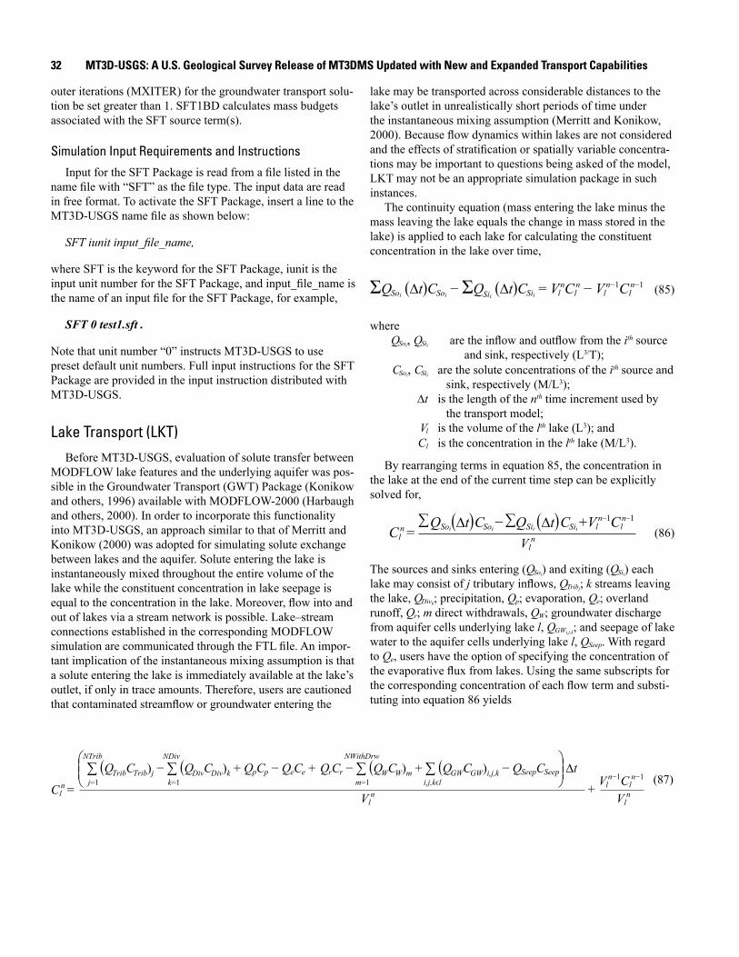
32 MT3D-USGS: A U.S. Geological Survey Release of MT3DMS Updated with New and Expanded Transport Capabilities
outer iterations (MXITER) for the groundwater transport solu-tion be set greater than 1. SFT1BD calculates mass budgets associated with the SFT source term(s).
Simulation Input Requirements and InstructionsInput for the SFT Package is read from a file listed in the
name file with “SFT” as the file type. The input data are read in free format. To activate the SFT Package, insert a line to the MT3D-USGS name file as shown below:
SFT iunit input_file_name,
where SFT is the keyword for the SFT Package, iunit is the input unit number for the SFT Package, and input_file_name is the name of an input file for the SFT Package, for example,
SFT 0 test1.sft .
Note that unit number “0” instructs MT3D-USGS to use preset default unit numbers. Full input instructions for the SFT Package are provided in the input instruction distributed with MT3D-USGS.
Lake Transport (LKT)Before MT3D-USGS, evaluation of solute transfer between
MODFLOW lake features and the underlying aquifer was pos-sible in the Groundwater Transport (GWT) Package (Konikow and others, 1996) available with MODFLOW-2000 (Harbaugh and others, 2000). In order to incorporate this functionality into MT3D-USGS, an approach similar to that of Merritt and Konikow (2000) was adopted for simulating solute exchange between lakes and the aquifer. Solute entering the lake is instantaneously mixed throughout the entire volume of the lake while the constituent concentration in lake seepage is equal to the concentration in the lake. Moreover, flow into and out of lakes via a stream network is possible. Lake–stream connections established in the corresponding MODFLOW simulation are communicated through the FTL file. An impor-tant implication of the instantaneous mixing assumption is that a solute entering the lake is immediately available at the lake’s outlet, if only in trace amounts. Therefore, users are cautioned that contaminated streamflow or groundwater entering the
lake may be transported across considerable distances to the lake’s outlet in unrealistically short periods of time under the instantaneous mixing assumption (Merritt and Konikow, 2000). Because flow dynamics within lakes are not considered and the effects of stratification or spatially variable concentra-tions may be important to questions being asked of the model, LKT may not be an appropriate simulation package in such instances.
The continuity equation (mass entering the lake minus the mass leaving the lake equals the change in mass stored in the lake) is applied to each lake for calculating the constituent concentration in the lake over time,
ΣQSoi (∆t)CSoi − ΣQSii (∆t)CSii = VlnCl
n − Vln−1Cl
n−1 (85)
where QSoi, QSii are the inflow and outflow from the ith source
and sink, respectively (L3/T); CSoi, CSii are the solute concentrations of the ith source and
sink, respectively (M/L3); ∆t is the length of the nth time increment used by
the transport model; Vl is the volume of the lth lake (L3); and Cl is the concentration in the lth lake (M/L3).
By rearranging terms in equation 85, the concentration in the lake at the end of the current time step can be explicitly solved for,
Cln =
(∆t)(∆t)Vl
n
Vln−1Cl
n−1CSiiQSiiCSoiQSoi +−∑∑ (86)
The sources and sinks entering (QSoi) and exiting (QSii) each lake may consist of j tributary inflows, QTribj; k streams leaving the lake, QDivk; precipitation, Qp; evaporation, Qe; overland runoff, Qr; m direct withdrawals, QW; groundwater discharge from aquifer cells underlying lake l, QGWi,j,k; and seepage of lake water to the aquifer cells underlying lake l, QSeep. With regard to Qe, users have the option of specifying the concentration of the evaporative flux from lakes. Using the same subscripts for the corresponding concentration of each flow term and substi-tuting into equation 86 yields
NTrib
j=1
NWithDrw
m=1 i,j,kϵl
NDiv
k=1∑ (QTribCTrib)j − ∑ (QDivCDiv)k + QpCp − QeCe + QrCr − ∑ (QWCW)m + ∑ (QGWCGW)i,j,k − QSeepCSeep
Cln =
∆t
+Vl
n Vln
Vln−1Cl
n−1 (87)

New Transport Packages Developed for MT3D-USGS 33
Equation 87 accommodates NTrib tributaries entering lake l. In applications with multiple streams or managed diversions flowing out of lake l, NDiv may be greater than 1. In these instances, CDiv = Cl
n. In a similar fashion, the concentration of each direct withdrawal, CW, from lake l, will be set equal to Cl
n. NWithDrw specifies the total number of direct withdrawals. Users have the option of entering non-zero concentrations for precipitation (Cp) and evaporation (Ce) as called for by the application. If values are not specified, Cp and Ce default to zero. Where groundwater is discharging to the lake (QGW), the concentration of the flux crossing the lake–aquifer interface is equal to the calculated concentration of the aquifer cell from which the discharge originates, QGWi,j,k. It is necessary to account for each cell discharging to a lake individually; the notation Σ
i,j,k ϵ l implies sum of each i,j,k index connected to the lth
lake. In contrast, wherever the lake is recharging the aquifer, the concentration of the lake seepage, CSeep, is equal to the calculated concentration of the lth lake, Cl
n. An important consideration to keep in mind when using
LKT is that MODFLOW allows lakes to coalesce and sepa-rate as stages rise and fall. This presents an additional level of calculation needed in the transport code that is unavailable with the first release of MT3D-USGS. Therefore, users who have simulated coalescing and separating lakes in their flow models are directed to GWT (Konikow and others, 1996) as an alternative until this functionality is added to MT3D-USGS.
Implementation in MT3D-USGSThe LKT Package consists of four primary subroutines,
LKT1AR, LKT1RP, LKT1FM, and LKT1BD, where the integer 1 indicates the new MT3D-USGS version number. LKT1AR allocates computer memory for data and working arrays after reading the user-specified input in the LKT input file. LKT1RP reads transient input data for the LKT Package. LKT1FM formulates and adds the LKT source term to the implicit finite-difference equations by adjusting the coefficient matrix, A, and right-hand side vector, RHS, as follows:
+=i,j,kGWLKi,j,ki,j,k QAA 11 −
RHSi,j,k = RHSi,j,k − Q+
where Q+GWLKi,j,k and Q−
GWLKi,j,k are the volumetric flow rates of groundwater/lake-water (GWLK) exchange, with “+” signify-ing seepage from the lake to the aquifer and “−” indicative of groundwater discharge to a lake for the cell(s) with indices i, j, and k. The concentration of the seeped lake water, CLK, is calculated by the LKT Package and will be updated with each outer iteration. LKT1BD calculates mass budgets associated with the LKT source term(s).
Simulation Input Requirements and InstructionsInput for the LKT Package is read from a file listed in the
name file with “LKT” as the file type. The input data are read in free format. To activate the LKT Package, insert a line to the MT3D-USGS name file as shown below:
LKT iunit input_file_name ,
where LKT is the keyword for the LKT Package, iunit is the input unit number for the LKT Package, and input_file_name is the name of an input file for the LKT Package, for example,
LKT 0 test1.lkt .
Note that unit number “0” instructs MT3D-USGS to use preset default unit numbers. Full input instructions for the LKT Package are provided in the input instruction distributed with MT3D-USGS.
Transport within the Unsaturated Zone
Morway and others (2013) document the expansion of MT3DMS to include unsaturated zone transport. That effort, referred to as “UZF-MT3DMS,” has been incorporated into MT3D-USGS. Transport in the unsaturated zone is facilitated by calculating volume-averaged water content on the basis of saturated and unsaturated water volumes in a finite-difference cell containing the water table. Under this assumption, water occupying the saturated portion of the cell is conceptual-ized as being “smeared” over the entire thickness of the cell (fig. 9), resulting in an equivalent water content that is used in the unsaturated-zone solute transport equations solved by MT3D-USGS. As a result of this approach, the calculated concentration in cells containing the water table is reflective
(88)
GWLKi,j,k CLK (89)
Figure 9. Saturated portion of a model cell (left) and its volume-averaged equivalent (right) in MT3D-USGS. An equivalent water content for cells containing the water table is calculated when the Unsaturated Zone Flow Package is active. The equivalent water content will be greater than the water content in the unsaturated portion of the cell but less than saturation, as a result of this approximation.

34 MT3D-USGS: A U.S. Geological Survey Release of MT3DMS Updated with New and Expanded Transport Capabilities
of the volume-averaged water content and is not meant to be interpreted as the concentration of water recharging the groundwater. In regional-scale problems using a relatively coarse vertical numerical grid, simulated arrival times of an infiltrating solute to the saturated zone could be the result of grid design, which does not accurately reflect the system it is meant to model. In non-point source applications wherein a ubiquitous contaminant persists, vertical grid refinement near the water table may be less of a concern.
The UZT Package relies on flux and storage terms cal-culated in the UZF1 (Niswonger and others, 2006) Package available in MODFLOW-2005 (Harbaugh, 2005) and MOD-FLOW-NWT (Niswonger and others, 2011). UZF1 solves unsaturated-zone flow processes using the method of charac-teristics technique to solve the kinematic wave approximation for one-dimensional downward vertical flow in the unsaturated zone. This approach neglects the diffusive term found in Richards’ equation (Richards, 1931), resulting in sharp wetting fronts and precludes the ability to simulate capillary pressures that draw water upward. However, the approach is numeri-cally efficient and stable; the method has provided reasonable results where Richards’ equation has historically struggled (Harman and others, 2011; McGrath and others, 2008a; McGrath and others, 2008b; Ross, 1990; Struthers and others, 2006; Van Dam and Feddes, 2000) and therefore is a viable alternative.
UZF1 uses the Method of Characteristics (MOC) (Smith and Hebbert, 1983; Smith, 1983) to solve the kinematic wave equation for routing flow through the unsaturated zone while also partitioning the infiltrating water into evapotranspiration (ET), recharge, runoff [either rejected infiltration (application rates in excess of the vertical hydraulic conductivity and (or) saturation induced runoff) or groundwater discharge (spring flow)], and unsaturated-zone storage changes. Because the discretization scheme within UZF1 is distinct from the MOD-FLOW grid, an intermediate step that maps the UZF1 fluid fluxes and calculated storage changes onto the MODFLOW grid for use by MT3D-USGS is required. MODFLOW’s LMT7 Package takes care of this intermediate step and records the appropriate values in the FTL file. To illustrate this, figure 10A shows two idealized (smooth) moisture contents at times t1 and t2, where t2 is greater than t1, and the corre-sponding step function (dashed lines) calculated and updated by UZF1 that approximates the idealized moisture content profiles. In figure 10B, the flux between layers 1 (L1) and 2 (L2) is greater than 0, whereas between L2 and L3, L3 and L4, and L4 and L5 there is no flux to record. The advancing wetting front has not yet crossed these layer interfaces, and the moisture within these cells is at residual. In figure 10C, a non-zero downward flux persists between L1 and L2, and between L2 and L3. The downward flux recorded in the FTL file will remain 0 between L3 and L4, and between L4 and L5. Owing
A CR S R S R S
B
Vertical griddiscretization
L1L1
L2L2
L3L3
L4L4
L5L5
L6L6
θS
θREXPLANATION
L1 Labels L1 to L6 indicate layer and number
Equivalent θmapped to
MODFLOW grid
θRθS
Wetting front at t1
Wetting/drying profile at t2
UZF1 approximation of wetting front at t1
UZF2 approximation of wetting/drying profile at t2
Residual water contentSaturated water content
Figure 10. A, two idealized wetting fronts moving downward through a uniform column of unsaturated material (smooth lines) that are approximated by step functions (dashed lines) using kinematic waves simulated with the Unsaturated Zone Flow Package (UZF1). Because wetting and drying waves are maintained by UZF1, which does not make use of the finite-difference grid, water content, θ, and between-layer fluxes must be mapped to the MODFLOW grid for use by MT3D-USGS. In B and C, the darker shades of blue indicate cells with higher moisture contents (θ closer to θs) than cells with lighter shades of blue (θ closer to θR). The discretization employed by UZF1 for simulating wetting and drying fronts will, in many model applications, be maintained at a finer resolution than the finite-difference grid. Therefore, multiple UZF1-calculated water contents may exist within the span of a single finite-difference cell. The equivalent water content that is passed to MT3D-USGS via the FTL file accounts for this heterogeneity.

New Transport Packages Developed for MT3D-USGS 35
to the trailing drying waves that form at t2, the volumetric flux rate between L1 and L2 will decrease in addition to the decrease in unsaturated-zone storage in L1.
In addition to UZF1-calculated fluxes and storage terms passed to MT3D-USGS via the FTL file, a few new user-specified inputs are required by the UZT Package. New inputs include initial saturated thickness and water contents entered into the UZT input file. Concentrations associated with the UZF1-related terms are entered in the UZT input file and include the concentration of (1) unsaturated-zone ET, (2) groundwater ET, and (3) surface leakage (that is, groundwater discharge). The ability to specify the constituent concentra-tion in ET flux is in keeping with traditional MT3DMS input formats. ET and surface leakage are the only types of sinks whose concentrations may be specified externally. The con-centration in ET occurring from the saturated and unsaturated zones defaults to zero if not specified by the user. In contrast, the concentration in spring discharge defaults to the calculated concentration in the groundwater in that cell. MT3D-USGS also requires that the ICBUND (see input instructions for description of ICBUND) array used to track the boundary con-dition type for each cell be set equal to 1 for partially saturated cells.
Readers are referred to the example models distributed with MT3D-USGS for exploring UZT functionality. When the UZT Package is active, MOC approaches available in saturated-only simulations (that is, MIXELM = 1, 2, or 3 in the ADV Package; see input instruction for description of MIXELM) cannot be used as they are left unsupported with version 1 of MT3D-USGS. Thus, users are limited to the implicit finite dif-ference and TVD solution techniques when using UZT.
Implementation in MT3D-USGSThe UZT Package consists of four primary subroutines,
UZT1AR, UZT1RP, UZT1FM, and UZT1BD, where the integer 1 indicates the new MT3D-USGS version number. UZT1AR allocates computer memory for data and working arrays after reading the user-specified input in the UZT input file. UZT1RP reads transient input data for the UZT Pack-age. UZT1FM formulates and adds the UZT source and sink terms to the implicit finite-difference equations depending on which of the four types of sources and sinks simulated by MODFLOW’s UZF1 Package are occurring in a cell. Infiltra-tion, unsaturated-zone ET, ET originating from the saturated zone, and groundwater discharge to land surface (for example, spring discharge) act as sources and sinks that adjust the coef-ficient matrix, A, and right-hand side vector, RHS, as follows:
A1i,j,k = A1
i,j,k + Q−si,j,k (90)
RHSi,j,k = RHSi,j,k − Q+si,j,k CINFi,j,k (91)
where Q+si,j,k and Q−
si,j,k are the volumetric flow rates of fluid sources (that is, infiltration) and sinks (that is, ET occurring from the unsaturated and saturated zones and groundwater
discharge to land surface), respectively. CINFi,j,k is the constitu-ent concentration in the infiltrating water at location i,j,k. The concentration in ET occurring from the saturated and unsaturated zones defaults to zero if not specified by the user. In contrast, the concentration in spring discharge defaults to the calculated concentration in the groundwater in that cell. UZT1BD calculates constituent mass budgets associated with the UZT source term(s).
Simulation Input Requirements and InstructionsInput for the UZT Package is read from a file listed in the
name file with “UZT” as the file type. The input data are read in free format. To activate the HSS Package, insert a line to the MT3D-USGS name file as shown below:
UZT iunit input_file_name ,
where UZT is the keyword for the UZT Package, iunit is the input unit number for the UZT Package, and input_file_name is the name of an input file for the UZT Package, for example,
UZT 0 test1.uzt .
Note that unit number “0” instructs MT3D-USGS to use preset default unit numbers. Full input instructions for the UZT Package are provided in the input instruction distributed with MT3D-USGS.
Incorporation of MODFLOW-2005 Array Utilities Options
The array reading utility functions included in the original release of MT3D had their own nuanced differences relative to the array readers included with MODFLOW. The MODFLOW array reader utility functions are included with MT3D-USGS. With the first release of MT3D-USGS, the MT3D- and MODFLOW-style array reader formats were available to the user. Note, however, that future releases of MT3D-USGS likely will not include the original MT3D-style array reader; instead MT3D-USGS likely will remain consistent with USGS-released versions of MODFLOW. A warning message is printed to the standard MT3D-USGS output file reminding users of this pending change in future versions of MT3D-USGS. Documentation of the MODFLOW-style array readers can be found on pages 8–57 of Harbaugh (2005). To enable MODFLOW-style array reader utilities in MT3D-USGS, enter the keyword “MODFLOWSTYLEARRAYS” on the first line of the BTN input file.

36 MT3D-USGS: A U.S. Geological Survey Release of MT3DMS Updated with New and Expanded Transport Capabilities
Benchmark Problems and Application Examples
A wide variety of benchmark problems are included with the MT3D-USGS distribution files. Reasons for including a large suite of benchmark problems are three fold. First, the models provide baseline benchmarks to verify that future code changes, by the USGS or otherwise, do not alter model results or performance. Second, model results discussed next for each of the benchmark models verifies that the code is working properly. Third, the included benchmarks serve as examples that demonstrate functionality of the MT3D-USGS program.
All of the model input files, whether associated with the MODFLOW or MT3D-USGS are provided among the MT3D-USGS distribution files. Those new to MODFLOW and MT3D are encouraged to familiarize themselves with the benchmark problems before pursuing larger, site-specific applications of their own.
The MT3D-USGS code has been tested with the bench-mark problems distributed with MT3DMS version 5.3. Doing so verified that the modifications and enhancements did not significantly alter the simulated results, except for cases where the revised storage formulation had an effect. Because backward-compatibility is maintained with the first release of MT3D-USGS, the original MT3DMS example models, as well as any existing MT3DMS simulation that does not rely on customized modifications, were run as-is using MT3D-USGS. Results from these benchmarks are not described in this report. Readers are directed to Zheng and Wang (1999) for additional information on those example problems.
Routing Mass Through Dry Cells
The model first published in Keating and Zyvoloski (2009) and described under the heading, “Extension to Mixed Vadose/Saturated Zone Simulations,” is solved with MODFLOW-NWT and MT3D-USGS to demonstrate the routing of solute mass through dry cells. In this problem, an aquitard above the underlying regional flow intercepts recharge and forms a perched aquifer. Under steady-state flow conditions, perched groundwater flows over the edges of the aquitard, and MOD-FLOW-NWT instantaneously applies this water to the top of the underlying aquifer. In the transport problem, the initial concentration is zero throughout the entire domain. Water entering and exiting the domain through the left and right boundaries, respectively, is assigned a concentration of 0. Only the recharge, specified in layer 1 (note that the highest active layer is 8) is specified with a non-zero concentration equal to 100 mg/L for the first 730 days of the simulation. Thus, the solute arrives first in the perched aquifer before eventually spilling over the sides of the aquitard and entering the lower aquifer. It is the new DRYCELL keyword functionality in MT3D-USGS that makes this type of simulation possible. Once in the lower aquifer, the solute is transported toward the
right boundary in response to groundwater flow patterns and in this way is routed through the perched and lower regional aquifers. Parameters for this model are given in table 3.
The MODFLOW-NWT simulation is steady-state; how-ever, 100 time steps, each 100 days long, are used in MT3D-USGS to represent the transient response of solute added to the top of the model. Figure 11 shows the migration of the plume at 100, 1,000, and 3,000 days (fig. 11A, B, and C, respectively). Once the solute reaches the lower aquifer, it migrates to the right. Figure 12 shows the breakthrough curves at two locations in the lower aquifer (fig. 11A), one below the left edge of the aquitard and the other near the right edge of the simulation, just upstream from the area where water exits the model. The standard output listing file shows the mass balance for the movement of mass through otherwise dry, and therefore inactive, cells in MT3D-USGS and confirms the mass concentration of the new functionality.
Table 3. Parameter values for a two-dimensional (2D) benchmark model simulating a perched aquifer intercepting and bifurcating contaminated recharge. [Aquifer properties are uniform except for the aquitard denoted in figure 12. ft, feet; ft/d, feet per day; mg/L, milligrams per liter]
Parameter Value
Cell width along rows (Δx) 25.0 ftCell width along columns (Δy) 25.0 ftAquifer hydraulic conductivity 0.8476 ft/dAquitard hydraulic conductivity 8.476 x 10⁻⁷ ft/dAnisotropy 1.0Porosity (ϕ; unitless) 0.10Recharge rate 0.072 ft/dRecharge concentration 100.0 mg/L

Benchmark Problems and Application Examples 37
Concentrations, in milligrams per liter0.01 0.10 0.50 0.90 0.99
2,000 4,000 6,000 8,000 10,0000
2,000
1,500
1,000
500
0
2,000
1,500
1,000
500
0
2,000
1,500
1,000
500
0
EXPLANATION
Saturated zone
Aquitard
Recharge boundary
Aquitard
Aquitard
A
B
C
See Figure 12A
See Figure 12B
Distance, in meters
Elev
atio
n, in
met
ers
100 days
1,000 days
3,000 days
Figure 11. Progression of a hypothetical plume that originates from recharge containing a solute in MT3D-USGS. A, 100 days after the solute first arrives in the perched aquifer. B, At 1,000 days, the solute has spilled over the sides of the aquitard and has migrated downward into the lower aquifer. C, After 3,000 days, the plume migrates toward the right model boundary.

38 MT3D-USGS: A U.S. Geological Survey Release of MT3DMS Updated with New and Expanded Transport Capabilities
0
0.1
0.2
0.3
0.4
0.5
0.6
0.7
0.8
Conc
entr
atio
n, in
mill
igra
ms
per l
iter
0 1,000 2,000 3,000 4,000 5,000 6,000 7,000 8,000Time, in hours
Conc
entr
atio
n, in
mill
igra
ms
per l
iter
Time, in hours
Keating and Zyvoloski (2009) resultsMT3D-USGS
0
0.02
0.04
0.06
0.08
0.10
0.12
0.14
0.16
0.18
0 5,000 10,000 15,000 20,000 25,000 30,000 35,000 40,000
A
B
EXPLANATION
Figure 12. Concentration breakthrough curves located A, within the lower regional aquifer below the left end of the aquitard and B, within the lower regional aquifer close to where groundwater flows out of the MODFLOW and MT3D-USGS simulations. Locations of the simulated breakthrough curves are shown in figure 11A. MT3D-USGS results are shown with results first published in Keating and Zyvoloski (2009).

Benchmark Problems and Application Examples 39
Instantaneous Electron Acceptor and Electron Donor Reaction
A simple example is presented to demonstrate the simula-tion of an ED in the presence of an EA and the instantaneous reaction that results. Results are compared to a known analyti-cal solution.
A single-cell numerical model was constructed with the cell length, width, and height being equal to 10 m with a constant porosity of 0.2 over the model domain. A transient flow and transport simulation was designed such that the volume of water in the model does not change with time. Thus, the initial saturated thickness is maintained throughout the simulation. To force this condition, water was injected at the same rate as water was removed by ET. The ET concentration remained at its default value of zero. As a result, the mass introduced to the system does not leave the model domain, and the volume of water in the model remains constant.
The transport simulation was performed with two solutes—the first an EA and the second an ED. In all of the benchmark problem variants described next, the initial concentration of the first acceptor species was set equal to 1,000 milligrams per cubic meter (mg/m3), whereas the initial concentration
of the second donor species was set equal to zero. Species 2 was introduced through the injection boundary at a rate of 2000 mg/d. Adding species two at this injection rate to the constant volume of 200 m3 supports a concentration build-up rate of 10 milligrams per cubic meter per day (mg/m3/d) in the absence of reactions.
The first variant of this benchmark problem held species 1 at the initial concentration and did not allow any reac-tion between the two species. Figure 13 shows the resulting concentration in the cell for species 1 and 2 and verifies that the initial and boundary conditions are simulated in the desired manner for the duration of the simulation. As a result, the con-centration of species 2 at the end of the simulation (500 days) is 5,000 mg/m3.
The next variant of the EA/ED benchmark problem is a modification of the first example that allows the two species to react with one another. The stoichiometric ratio between the two simulated constituents was set equal to 1.0, meaning that a unit of species 1 consumes a unit of species 2. The simulated concentration is shown in figure 14 where it can be seen that species 2 consumes species 1 until it is completely consumed at 100 days. After this time, the concentration of species 2 accumulates at the injection rate of 10 mg/m3/d.
Time, in days0 100 200 300 400 500
0
2,000
2,500
1,000
1,500
500
3,000
3,500
4,000
4,500
5,000
Conc
entr
atio
n, in
mill
igra
ms
per c
ubic
met
er
MT3D-USGS species 1MT3D-USGS species 2
EXPLANATION
Figure 13. Concentrations of species 1 and 2 with no inter-species reactions simulated during the modeled period in MT3D-USGS.

40 MT3D-USGS: A U.S. Geological Survey Release of MT3DMS Updated with New and Expanded Transport Capabilities
Time, in days0 100 200 300 400 500
0
2,000
2,500
1,000
1,500
500
3,000
3,500
4,000
4,500
5,000
Conc
entr
atio
n, in
mill
igra
ms
per c
ubic
met
er
MT3D-USGS species 1MT3D-USGS species 2
EXPLANATION
Figure 14. Concentrations of species 1 and 2 are shown for the problem where inter-species reactions take place using a stoichiometric ratio of 1.0 in MT3D-USGS.
The third and final variant of the EA/ED benchmark problem modified the stoichiometric ratio to 2.0, meaning that 1 unit of species 1 is consumed by 2 units of species 2. In so doing, the time to total consumption of species 2 is doubled and now occurs 200 days after the start of the simulation (fig. 15). As with the first two variants of this benchmark prob-lem, the concentration of species 2 builds up at the injection rate (10 mg/m3/d) after species 1 is completely consumed.
Multiple EA and ED Reactions: Verification of Implementation
Verification of the new reaction package implementa-tion within MT3D-USGS is demonstrated with two example problems.
Benchmark using Independent Reaction Program and RT3D
The first example is designed to verify that the reaction module was correctly coupled with MT3D-USGS and is cor-rectly executed by MT3D-USGS at run-time. The problem was first described by Lu and others (1999) and is solved with RT3D when simulating a single ED. This benchmark example ensures that MT3D-USGS, incorporating parent-daughter reactions, matches RT3D results when simulating a single ED
and employing transport variables and options analogous to those offered by the RT3D program.
A simple two-cell MODFLOW model was used to provide a FTL file suitable for use with both MT3D-USGS—incor-porating the new reaction package—and RT3D. Using a flow model that simulates no net flow and executing both MT3D-USGS and RT3D using only their respective Source-Sink Mix-ing (SSM) and Reaction (RCT) Packages (that is, neglecting dispersion), the calculations performed by MT3D-USGS and RT3D are essentially isolated “batch” reaction calculations. As such, for a single ED and five EAs, including the use of Fe(II) and methane (as described in the section “Kinetic Reac-tion Between Multiple Electron Donors and Acceptors”), as employed by RT3D, MT3D-USGS incorporating the reaction module should produce results identical to those from RT3D.
Table 4 lists the transport parameters specified for use in this benchmark analysis. Figure 16 shows plots of the degrada-tion of the single ED in the presence of multiple EAs, as cal-culated by MT3D-USGS, incorporating the reaction equations as a subroutine and RT3D. Because the equations developed in the earlier sections used benzene as an example reactant, in this example BTEX is the constituent being simulated and is predominantly composed of benzene. A comparison of the results clearly shows that when MT3D-USGS uses equivalent treatments for iron and methane as RT3D, the results are iden-tical between the two programs.

Benchmark Problems and Application Examples 41
Time, in days0 100 200 300 400 500
0
2,000
2,500
1,000
1,500
500
3,000
3,500
4,000
4,500
5,000
Conc
entr
atio
n, in
mill
igra
ms
per c
ubic
met
ers
MT3D-USGS species 1MT3D-USGS species 2
EXPLANATION
Figure 15. Concentrations of species 1 and 2 are shown for the problem where between-species reactions take place using a stoichiometric ratio of 2.0 in MT3D-USGS.
Table 4. Transport parameters specified in MT3D-USGS benchmark simulations.[BTEX, benzene toluene ethylbenzene and xylene; O2, oxygen; NO3, nitrate; Fe2+, iron(II); SO4, sulfate; CH4, methane; n/a, not applicable]
Species Initial concentration
Yield coefficient
Inhibition constant
Half saturation constant
Maximum expressible
concentrationDecay rate
BTEX 10.0 n/a n/a n/a n/a 0.00168O2 6.0 3.14 0.01 0.5 n/a 0.00168NO3 17.0 4.9 0.01 0.5 n/a 0.00168Fe2+ 0.001 -21.8 0.01 0.5 50.5 0.00168SO4 100 4.7 0.01 0.5 n/a 0.00168CH4 0.0001 -0.78 n/a 0.5 2.05 0.00168

42 MT3D-USGS: A U.S. Geological Survey Release of MT3DMS Updated with New and Expanded Transport Capabilities
Time, in hours
0 500 1,000 1,500 2,000 3,0002,500
Conc
entr
atio
n, in
mill
igra
ms
per l
iter
Met
hane
con
cent
ratio
n, in
10–4
mill
igra
ms
per l
iter
0
0.5
1.0
1.5
2.0
3.0
2.5
0
20
40
60
80
100
120
RT3D, volatile organic compoundsRT3D, oxygenRT3D, nitrateRT3D, ironRT3D, sulfateRT3D, methaneEquivalent MT3D-USGS (by color)
EXPLANATION
RT3D, Reactive Transport in 3 Dimensions program
Figure 16. Plots for the benchmark simulation of a single electron donor in the presence of multiple electron acceptors simulated using MT3D-USGS and RT3D. The spacing between MT3D-USGS simulated equivalents (denoted by “x”) does not imply time-step length; intermittent simulated equivalents are plotted to reduce clutter.
Benchmark of a Multiple Electron Donor Case: A Mass Balance Approach
Because the published version of RT3D considers the degradation of a single ED, it is not possible to use RT3D to verify the simulation of more than one ED. Therefore, the sec-ond benchmark exercise consists of a simple simulation aimed at identifying whether the multiple-ED reaction equations execute as expected.
This benchmark is based on the premise that the consump-tion of EAs by a single ED that has an initial concentration of 1.0 unit should be equivalent (at least, until such time as diminishingly small concentrations occur) to the consump-tion of EAs by two EDs that have an initial concentration of 0.5 unit. That is, it is assumed that in the general case the effect of one ED is equivalent to the summed effect of two EDs that have equivalent properties.
The transport parameters specified for use in this bench-mark analysis (table 4) are identical to those used in the first benchmark simulation. Figure 17 shows the plots of the deg-radation of the two EDs in the presence of multiple EAs cal-culated by MT3D-USGS incorporating the reaction equations as a subroutine. Also plotted is the degradation of the single
ED in the presence of the same EAs; degradation was calcu-lated by the stand alone reaction program. Review of figure 17 reveals that, as expected by inference, the consumption of EAs by two EDs that possess initial concentrations of 0.5 units is equivalent to the consumption of EAs by one ED that has an initial concentration of 1.0 unit.
Two-Dimensional Application ExampleThe next example is a two-dimensional demonstration that
is based upon the applications described in this report and the linkage of the Kinematic Oily Pollutant Transport (KOPT) and the OILENS (Weaver and others, 1994) modules of the original HSSM program to MT3DMS (Zheng and others, 2008). However, in the current example application, each of the two sources of contaminants is considered to consist of a multi-component LNAPL, represented in this example as a single ED; the reactive transport of a subset of these com-ponents is simulated. The example simulation is a simplified two-dimensional flow-and-transport problem, which demon-strates that the new MT3D-USGS reaction package achieves three functions.

Benchmark Problems and Application Examples 43
Time, hours
0 500 1,000 1,500 2,000 3,0002,500
Conc
entr
atio
n, in
mill
igra
ms
per l
iter
Met
hane
con
cent
ratio
n, in
10–4
mill
igra
ms
per l
iter
0
0.5
1.0
1.5
2.0
3.0
2.5
0
20
40
60
80
100
120
RT3D, volatile organic compounds*RT3D, oxygenRT3D, nitrateRT3D, ironRT3D, sulfateRT3D, methaneEquivalent MT3D-USGS (by color)
* Represented by 2 electron donors in MT3D-USGS
EXPLANATIONRT3D, Reactive Transport in 3 Dimensions program
Figure 17. Plots for the benchmark simulation of two electron donors in the presence of multiple electron acceptors simulated using RT3D and MT3D-USGS.
1. MT3D-USGS correctly loads the parameters that define the transport characteristics of the multiple components.
2. It accurately solves the transient mass-transport equation using the GCG solver to implicitly update the source matrix over time.
3. It simulates the degradation of the electron donor (ED), and consumption of the electron acceptors and the gen-eration of products emanating from electron acceptors (both commonly referred to as EAs). The terms EDs and EAs are used to demonstrate the generic nature of the reaction package added to MT3D-USGS.
A hypothetical subsurface release of a gasoline fuel is simu-lated using (1) a simple advective-dispersive transport model and (2) the new MT3D-USGS reactive transport code. For the latter, transport of a single ED and five EAs is simulated. Aquifer and transport parameters used for this benchmark simulation are listed in table 5. Reactive transport parameters associated with the new package are listed in table 6. The input instructions distributed with the source code and model executable provide additional detail for formatting multiple EA/ED input files.
Table 5. Parameter values for a two-dimensional (2D) benchmark model simulating an electron donor and multiple electron acceptors. [ft/d, feet per day; ft, feet]
Parameter Value
Hydraulic conductivity 200 ft/d
Recharge 1.67 ft/d
Porosity (ϕ; unitless) 0.3
Longitudinal dispersivity (unitless) 6.63
Transverse dispersivity 0.663 ft
The model domain is a regular finite difference grid com-posed of 1 layer, 161 rows, and 161 columns (fig. 18). The flow field (that is hydraulic gradient) is maintained constant throughout the simulation using constant head (Dirichlet) conditions on the upgradient (right) and downgradient (left) boundaries. The TVD scheme is used to solve the advection component of the partitioned transport equation to minimize numerical dispersion (Zheng and Wang, 1999). The dissolved phase concentration of the arbitrary ED is monitored at a hypothetical monitoring (receptor) well placed downgradient

44 MT3D-USGS: A U.S. Geological Survey Release of MT3DMS Updated with New and Expanded Transport Capabilities
Table 6. Reactive transport parameter values for a two-dimensional (2D) benchmark model simulating an electron donor and multiple electron acceptors. [EA, electron acceptor; ED, electron donor; n/a, not applicable]
Constituent Decay rate Yield coefficient
Inhibition constant
Initial concentra-
tion
Electron acceptor 1 (EA1) -0.008 25 0.01 1
Electron acceptor 2 (EA2) -0.008 50 0.01 1
Electron acceptor 3 (EA3) -0.008 -5 0.01 0.01
Electron acceptor 4 (EA4) -0.008 300 0.01 1
Electron acceptor 5 (EA5)1 -0.008 -15 n/a 0.1
Electron donor 1 (ED1) n/a 0 n/a 2101Product of an electron accepting reaction, demonstrating the effect of the base electron
acceptor on consuming the ED.2Source concentration (initial concentration is 0).
from the north LNAPL source. In this simulation, the sources are identical, and results, including breakthrough curves and plume extents (figs. 19 and 20, respectively), are shown for the upper source (fig. 18) only. The total simulation time is 100 days. The source is activated at t=0.0 days (that is at time zero).
Because the purpose of this example is to demonstrate that the new reaction package is working as expected, parameter values associated with the new package were chosen fairly arbitrarily in order to clearly demonstrate that the developed code simulated degradation of the ED, consumption of EAs 1, 2, and 4 (notionally representing oxygen, nitrate, and sulfate) and the effect of EAs (notionally representing the ferric iron and organic carbon) represented by the production of reaction products of EAs 3 and 5 (notionally representing the ferrous iron and methane). EAs 1, 2, and 4 had different positive yield coefficients to demonstrate consumption of EAs at different
Groundwater flowGroundwater flow
Simulated source (not to scale)Receptor (monitoring well) (not to scale)Constant head
EXPLANATION
Figure 18. Two-dimensional hypothetical model domain with the location of principal features in MT3D-USGS.

Benchmark Problems and Application Examples 45
Time, in hours
Conc
entr
atio
n, E
As,
in m
illig
ram
s pe
r lite
r
Conc
entr
atio
n, E
D, i
n m
illig
ram
s pe
r lite
r
0
0.2
0.4
0.6
0.8
1.0
1.2
0
1
2
3
4
5
6
7
8
0 20 40 60 80 100
Electron donor (ED) (Reaction)Electron donor (No reaction)Electron acceptor (EA) 1Electron acceptor 2Electron acceptor 3Electron acceptor 4Electron acceptor 5
EXPLANATION
EA, electron acceptor; ED, electron donor
Figure 19. Breakthrough curves at receptor calculated using the multi-species MT3D-USGS transport code with reaction (solid black line) and without reaction (dashed black line).
Time (t) = 50 days
Time (t) = 100 days
SourceElectron acceptor (EA) 1Electron acceptor 2Electron acceptor 3Electron acceptor 4Electron acceptor 5Electron donor (ED) (non-reactive)Electron donor (reactive)Receptor well
Low High
EXPLANATION
A
B
Concentration of ED [benzene toluene ethylbenzene xylene (BTEX)]
EA, electron acceptor; ED, electron donor; BTEX, benzene toluene ethylbenzene xylene
multi-species MT3D-USGS code. Figure 20. Extent of electron donor, BTEX, plume at 50 and 100 days calculated A, without and B, with reactive transport using the

46 MT3D-USGS: A U.S. Geological Survey Release of MT3DMS Updated with New and Expanded Transport Capabilities
rates. EAs 3 and 5 had different negative yield coefficients to demonstrate production of these products resulting from EA reactions at different rates.
The concentration breakthrough curves at the receptor well for the ED and each of the 5 EAs is presented in figure 19. A comparison of the reactive and the non-reactive ED break-through curves in figure 19 reveals that the ED was consumed. The amount of consumption (the difference between these two curves) is controlled by the decay rate used for each EA. In addition, the consumption or production of the different EAs and their products occurred in correspondence with their order in the input file. For example, consumption of EA1 occurred first, followed by EA2.
The areal extents of the ED and the EAs after 50 days and 100 days are presented in figure 20. Arbitrary contour intervals are used to clearly depict the ED degradation and EA consumption/production. The contour level for the ED corresponds to a concentration of 0.001 mg/L. The contour levels for the EAs that are consumed correspond to a concen-tration of 0.95 mg/L, which in turn corresponds to 5-percent consumption from the original concentration of 1.0 mg/L. The extents of the EAs representing the product of electron accep-tors that are produced correspond to a concentration value slightly higher than their initial concentrations. For EA3, this concentration is 0.015 mg/L, and for EA5 this concentration is 0.11 mg/L.
As expected, the extent of the ED plume under reactive conditions is less than its extent under non-reactive condi-tions. The difference is small because only a relatively small fraction (about 5%) of the ED was degraded in this simulation (see fig. 19). The extent of EA1 depletion is the largest of the EAs, followed by EA2, EA3, EA4, and EA5. The extent of EA4 depletion is greater than that of EA3 because its yield coefficient is significantly greater. That is, after EA4 begins to degrade, it does so at a greater rate. As expected, the extents of each of the plumes increased between the 50 and 100 days owing to the longer migration time.
Contaminant Treatment System Benchmark Problems
The benchmark problems designed for the new CTS mod-ule serves a four-fold purpose. First, the benchmark problems ensure that mass is preserved under each of the treatment options. Second, each treatment option also provides a bench-mark for testing future CTS enhancements. Third, the CTS benchmark models provide an input format template. Fourth, the benchmark models demonstrate the effect of each of the available treatment options on the final solution. All four of the benchmark models use the same model setup—a cluster of four extraction wells on the left side of the model domain and four injection wells on the right (fig. 21). Contaminated water
C = 40, concentration is 40 milligrams per liter (mg/L); C = 60, 60 mg/L; C = 80, 80 mg/L; C = 100, 100 mg/L
Well 1
Well 2
Well 3
Well 4
Well 5
Well 6
Well 7
Well 8
C = 40
C = 60
C = 80
C = 100
Prescribed concentration
Extraction well
Injection well
Constant-head boundary
EXPLANATION
Figure 21. Model grid representing the Contaminant Treatment System Package benchmark problem and the positions of injection and extraction wells.

Benchmark Problems and Application Examples 47
extracted from the aquifer and collected in one of the two treatment systems included in benchmark simulations receives various treatment for testing each of the available treatment options. The treatment systems present users with an option to treat extracted water or to leave it untreated. In addition, extracted water may be blended or left unblended before being sent back to the injection wells. The various treatment options for the extracted water are also explored in the discussion of the benchmark simulations that follow.
CTS Benchmark Simulation 1The first CTS benchmark problem tests whether the CTS
module was implemented as intended. Four extraction wells withdraw contaminated water in a confined single layer model. Four injection wells simultaneously inject contaminated water back into the confined aquifer at the injection sites. For verifi-cation purposes, results from the CTS simulation are com-pared with predicted output from a simulation that uses the Source-Sink Mixing (SSM) Package of MT3DMS to represent a simplified treatment option.
The numerical grid consists of 31 rows, 31 columns, and 1 layer. Spatial and temporal discretization of the model is pro-vided in table 7. Note that this recirculation simulation is an extension of a benchmark problem described in Section 7 of the MT3DMS manual (Zheng and Wang, 1999). Note the four prescribed concentration cells (with specified concentrations, from top to bottom, of 40, 60, 80, and 100 mg/L, respectively)
next to the extraction wells (fig. 21) that serve as the source of the aquifer contamination. Use of the specified concentration cells forces a known concentration to enter the CTS systems and facilitates verification of the treatment system. During stress period two, the prescribed concentration cells are altered such that their concentrations, from top to bottom respectively, are 30, 50, 70, and 90 mg/L. This forces the concentration in the extraction well to respond to transient boundary conditions and once again enables quick viewing of the model response to ensure that it is working as expected. Extracted water is treated by one of two treatment systems, as alluded to above, and injected into the aquifer via the injection wells. Table 8 shows the rates of extraction and injection for each of the eight wells.
The baseline simulation invoking SSM, to which CTS results are compared, extracts water from the model with a constituent concentration equal to the simulated constituent concentration in groundwater from which water is withdrawn. Moreover, the constituent concentration in the injected water is prescribed as 50 and 60 mg/L during the first and second stress periods, respectively. Figure 22 depicts a conceptual representation of this setup. Note the use of two CTS sys-tems; the first exports the contaminated groundwater from the simulation, thereby emulating the extraction boundary condi-tions imposed by the pumped wells in the SSM simulation. The second CTS system pumps water back into the aquifer
Table 7. Flow and transport model input parameters. [ft, feet; ft/s, feet per second; yr, year]
Model parameter Value
Cell width along rows (Δx) 900 ft
Cell width along columns (Δy) 900 ft
Layer thickness (Δz) 20 ft
Hydraulic conductivity of the aquifer (K) 0.005 ft/s
Porosity (ϕ; unitless) 0.3
Longitudinal dispersivity (αL) 100 ft
Ratio of transverse to longitudinal dispersivity (αL/ αT) 1.0
Length of the first stress period 2.5 yr
Length of the second stress period 7.5 yr
Table 8. Simulated pumping rates in the Contaminant Treatment System (CTS) benchmark simulation. [ft3/s, cubic feet per second]
Well number
Pumping rate (ft3/s) 1
Stress period 1 (912.5 days)
Stress period 2 (2,737.5 days)
1 -5.0 -6.0
2 -3.0 -4.0
3 -2.0 -3.0
4 -1.0 -2.0
5 0.5 1.5
6 1.5 2.5
7 3.5 4.5
8 5.5 6.51Negative rates indicate extraction, whereas positive rates indicate injection.
Extraction pumping rates and associatedconcentration as boundary condition
Extraction wells
Q1, Q2, Q3, Q4C1, C2, C3, C4
Injection wells
Q5, Q6, Q7, Q8C5, C6, C7, C8
Land surface
Injection pumping rates and associatedconcentration as a boundary condition
Figure 22. Conceptual representation of the baseline Source-Sink Mixing Package simulated pumping and injection boundary conditions used to verify the Contaminant Treatment System simulation.

48 MT3D-USGS: A U.S. Geological Survey Release of MT3DMS Updated with New and Expanded Transport Capabilities
via the four injection wells at constituent concentration levels described previously and in so doing mimics the injection wells in the SSM simulation. Figure 23 shows how each CTS is configured in this simulation.
Breakthrough curves at the well locations as predicted by the SSM baseline and CTS simulation are compared for assessing the performance of the CTS Package. Figure 24 shows the extraction well breakthrough curves for both
simulations. The first stress period extends from 0 to 912.5 days, at which point the second stress period begins. Results presented in figure 24 show that the CTS Pack-age is working as expected. The concentration of the water extracted from wells 1 through 4 (fig. 21) drops in response to a 10 mg/L lowering of the specified concentration cells. Similarly, the four injection well breakthrough curves high-light excellent agreement between the baseline SSM and CTS simulations (fig. 25).
Treatment System 1
Treatment System 2
Implemented route in example
Possible route not implemented in example
Injection wellsExtraction wells
Injection wellsExtraction wells
QesnkCesnk
QesrcCesrc
QesnkCesnk
QesrcCesrc
EXPLANATION
Q1 Q2 Q3 Q4C1 C2 C3 C4
Q5 Q6 Q7 Q8C5 C6 C7 C8
Q1 Q2 Q3 Q4C1 C2 C3 C4
Q5 Q6 Q7 Q8C5 C6 C7 C8
Qesrc Flow entering simulation domain from an external sourceQesnk Flow exported from the simulation domain to an external sinkQ1 Flow pumped from well 1Q2 Flow pumped from well 2Q3 Flow pumped from well 3Q4 Flow pumped from well 4Q5 Flow injected into well 5Q6 Flow injected into well 6Q7 Flow injected into well 7Q8 Flow injected into well 8Cesrc Concentration of flow entering the simulation domain from an external sourceCesnk Concentration of flow exported from the simulation domain to an external sinkC1 Concentration of flow pumped from well 1C2 Concentration of flow pumped from well 2C3 Concentration of flow pumped from well 3C4 Concentration of flow pumped from well 4C5 Concentration of water injected into well 5C6 Concentration of water injected into well 6C7 Concentration of water injected into well 7C8 Concentration of water injected into well 8
Figure 23. Conceptual routing of water and contaminant in the Contaminant Treatment System simulation. Extracted water is exported during the simulation by the first Contaminant Treatment System (CTS), whereas the second CTS (Treatment System 2) injects water at a prescribed concentration.
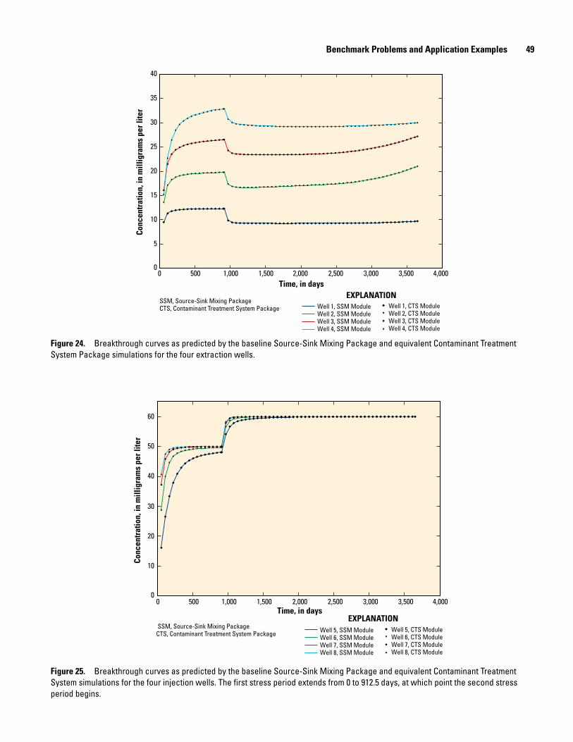
Benchmark Problems and Application Examples 49
Time, in days0 500 1,000 1,500 2,000 3,0002,500 4,0003,500
Conc
entr
atio
n, in
mill
igra
ms
per l
iter
0
5
10
15
20
25
30
35
40
Well 1, SSM ModuleWell 2, SSM ModuleWell 3, SSM ModuleWell 4, SSM Module
Well 1, CTS ModuleWell 2, CTS ModuleWell 3, CTS ModuleWell 4, CTS Module
EXPLANATIONSSM, Source-Sink Mixing PackageCTS, Contaminant Treatment System Package
Figure 24. Breakthrough curves as predicted by the baseline Source-Sink Mixing Package and equivalent Contaminant Treatment System Package simulations for the four extraction wells.
Time, in days0 500 1,000 1,500 2,000 3,0002,500 4,0003,500
Conc
entr
atio
n, in
mill
igra
ms
per l
iter
0
10
20
30
60
50
40
Well 5, SSM ModuleWell 6, SSM ModuleWell 7, SSM ModuleWell 8, SSM Module
Well 5, CTS ModuleWell 6, CTS ModuleWell 7, CTS ModuleWell 8, CTS Module
EXPLANATION SSM, Source-Sink Mixing PackageCTS, Contaminant Treatment System Package
Figure 25. Breakthrough curves as predicted by the baseline Source-Sink Mixing Package and equivalent Contaminant Treatment System simulations for the four injection wells. The first stress period extends from 0 to 912.5 days, at which point the second stress period begins.

50 MT3D-USGS: A U.S. Geological Survey Release of MT3DMS Updated with New and Expanded Transport Capabilities
During each of the stress periods, the constituent concentration in the extracted water begins to rise in response to the con-taminated injection water. At the four injection well locations (that is, wells 5, 6, 7, and 8), constituent concentrations in groundwater approach the prescribed injection concentrations of 50 and 60 mg/L during the first and second stress periods, respectively. Constituent mass budgets for the baseline SSM and CTS simulations are identical.
Additional CTS Benchmark SimulationsThe next several benchmark problems are presented to
demonstrate the simulation of various treatment options avail-able in the CTS Package. The same model setup as shown in figure 21 is used in the following examples; however, the configuration of the two treatment systems is altered (fig. 26). To highlight some of the CTS capabilities, the flow rates at extraction and injection wells associated with the two treat-ment systems are altered between stress periods. During the
first stress period, extraction wells 1, 2, and 4 are connected to treatment system 1. Extraction well 3 is connected to treat-ment system 2. Effluent from treatment system 1 is injected into wells 7 and 8, whereas effluent from treatment system 2 is injected into wells 5 and 6. In stress period 2, treatment system 1 treats water from well 1 and subsequently injects its effluent into wells 5 and 7. Treatment system 2 treats water extracted from wells 2, 3, and 4 and then injects the treated effluent into wells 6 and 8. In this particular set of benchmark problems, there are no external sources or sinks of mass to and from the treatment systems.
Five simulations were run to introduce and verify vari-ous treatment options available in the CTS Package. In the first simulation, no treatment was provided by either of the treatment systems. Figure 27 shows the resulting break-through curves at each of the four injection wells using the no treatment option. The first stress period extends from 0 to 912.5 days, at which point the second stress period begins. The MT3D-USGS solution was compared to simulated values
TreatmentSystem 1
TreatmentSystem 1
TreatmentSystem 2
TreatmentSystem 2
Stress period 1 Stress period 2
Injection wellsInjection wellsExtraction wells Extraction wells
Q1 Q2C1 C2
Q1C1
Q7 Q8C7 C8
Q4C4
Q5 Q7C5 C7
Injection wellsInjection wellsExtraction wells Extraction wells
Q2 Q3 Q4C2 C3 C4
Q5 Q6C5 C6
Q3C3
Q6 Q8C6 C8
Implemented route in example
EXPLANATION
Q1 Flow pumped from well 1Q2 Flow pumped from well 2Q3 Flow pumped from well 3Q4 Flow pumped from well 4Q5 Flow injected into well 5Q6 Flow injected into well 6Q7 Flow injected into well 7Q8 Flow injected into well 8
C1 Concentration of flow pumped from well 1C2 Concentration of flow pumped from well 2C3 Concentration of flow pumped from well 3C4 Concentration of flow pumped from well 4C5 Concentration of water injected into well 5C6 Concentration of water injected into well 6C7 Concentration of water injected into well 7C8 Concentration of water injected into well 8
Figure 26. Well configuration for the two treatment systems for stress periods 1 and 2 in the Contaminant Treatment System simulation.

Benchmark Problems and Application Examples 51
Time, in days0 500 1,000 1,500 2,000 3,0002,500 4,0003,500
Conc
entr
atio
n, in
mill
igra
ms
per l
iter
Well 5, MT3D-SSPAWell 6, MT3D-SSPAWell 7, MT3D-SSPAWell 8, MT3D-SSPA
Well 5, MT3D-USGSWell 6, MT3D-USGSWell 7, MT3D-USGSWell 8, MT3D-USGS
0
5
10
15
20
25
30
35
EXPLANATIONS.S. Papadopulos & Associates (SSPA) is the solution calculated using a code developed in a collaborative effort between CH2M and SSPA (CH2M Hill Plateau Remediation Company, 2010). Locations of the four extraction wells are shown in figure 21
Figure 27. Constituent concentrations for the four injection wells with no treatment administered.
generated by a previously published code, referred to as MT3D-SSPA, a version of MT3D maintained by S.S. Papa-dopulos & Associates (SSPA) and developed in a collabora-tive effort between CH2M and SSPA (CH2M Hill Plateau Remediation Company, 2010). It is important to note that the constituent concentrations shown in figure 27 correspond to the concentration of the injected water and not the simulated concentration in the aquifer. In this example, the concentra-tions in the wells are higher than the simulated concentrations in the aquifer. Concentrations in the aquifer are reflected by the concentrations in the water removed by the extraction wells, as shown in figure 28.
During stress period 1 of the “no treatment” option, water of time-varying quality is extracted from wells 1, 2, and 4 by treatment system 1 (fig. 26). Next, the collected water is blended and injected into wells 7 and 8. Water pumped from well 3 is circulated through treatment system 2 and injected into wells 5 and 6. It is no surprise that the concentrations in injection wells 7 and 8 are identical as they receive the same blend of water extracted from wells 1, 2, and 4. Similarly, concentrations in injections wells 5 and 6 are identical and are the same as concentrations noted in extraction well 3 in stress period 1. At the outset of stress period 2, the configuration of wells for treatment systems 1 and 2 is changed, as shown in figure 26. The concentrations in injection wells 5 and 7 are identical to the concentration of water extracted from well 1
during stress period 2. The concentrations in water injected into wells 6 and 8 result from the blending of water extracted from wells 2, 3, and 4.
The next four simulations use the configuration just described but have different treatment options selected to dem-onstrate the “out-of-the-box” functionality provided in CTS. Treatment options can either be applied to an entire treatment system, effectively providing treatment to all of the wells serviced by that treatment system, or well-specific treatment can be pursued where needed. Table 9 summarizes the type of treatments simulated in benchmark simulations that follow.
Table 9. An example of four types of Contaminant Treatment System (CTS) treatments available. [CTS treatments are applied to benchmark simulations. IOPT, variable name for selec-tion of treatment option; %, percent; mg/L, milligrams per liter; kg/d, kilograms per day]
Treatment option (IOPT)
Description
1 Treatment with 50% efficiency (50% concentration/mass removal)
2 Specified concentration reduction of 10 mg/L
3 Specified mass removal of 28.3 kg/d
4 Concentration treatment to a specified level of 15 mg/L only if the blended concentration exceeds 15 mg/L

52 MT3D-USGS: A U.S. Geological Survey Release of MT3DMS Updated with New and Expanded Transport Capabilities
Time, in days0 500 1,000 1,500 2,000 3,0002,500 4,0003,500
Conc
entr
atio
n, in
mill
igra
ms
per l
iter
0
5
10
15
20
25
30
35
Well 1, MT3D-SSPAWell 2, MT3D-SSPAWell 3, MT3D-SSPAWell 4, MT3D-SSPA
Well 1, MT3D-USGSWell 2, MT3D-USGSWell 3, MT3D-USGSWell 4, MT3D-USGS
EXPLANATIONS.S. Papadopulos & Associates (SSPA) is the solution calculated using a code developed in a collaborative effort between CH2M and SSPA (CH2M Hill Plateau Remediation Company, 2010). Locations of the four extraction wells are shown in figure 21
Figure 28. Simulated constituent concentrations for four extraction wells using the Contaminant Treatment System Package. There is no treatment in this simulation. The first stress period extends from 0 to 912.5 days, at which point the second stress period begins.
Results for injection well 5 for each of the simulated treatment options are shown in figure 29. The “no treatment” option originally plotted in figure 27 for well 5 is replotted in figure 29 (blue line) and serves as the baseline to which the other results can be compared. Readers are reminded that “no treatment” results in the blended concentration being sent out to injection wells connected to such treatment systems.
The first treatment option removes 50 percent of the mass (or concentration) from the blended water. Thus, the con-centration in well 5 is half that of the “no treatment” option results. Under the second treatment (IOPT=2), the resulting concentration in well 5 is 10 mg/L less than the simulated “no treatment” option results. During the second stress period, the requested 10-mg/L reduction of the injected water is reduced such that it equals the concentration of the blended water in the treatment system because negative concentrations can-not occur. The third treatment option (IOPT=3) simulates the removal of 28.3 kg/d of mass from the blended water before it is injected. Figure 29 shows the effect this treatment has on the concentration of the injected water. Finally, under the fourth treatment option (IOPT=4), the concentration of the injected water is set equal to 15 mg/L, meaning that the treatment sys-tem removed mass from the pumped and blended water such that its concentration prior to injection is equal to 15 mg/L. During the second stress period the baseline concentration falls below 15 mg/L even without treatment; it is no surprise,
then, that the concentration in the injected water in IOPT=4 is equal to the original “no treatment” concentration calculated for this stress period.
SFT and LKT Benchmark Problems
To demonstrate the utility and accuracy of the SFT and LKT functionality, three benchmark problems are described. The first problem compares MT3D-USGS output for an SFT-only simulation in which groundwater is entering a stream. In the second benchmark problem, a LKT-only simulation is presented to verify accurate simulation of lake concentrations assuming instantaneous mixing throughout the lake. The third benchmark problem originally appeared in Merritt and Koni-kow (2000) under the heading “Test Simulation 4: Simulation of Solute Concentrations,” then again in Prudic and others (2004) under the heading “Test 2: Stream-Lake Interaction with Solute Transport.”
Streamflow Transport with Groundwater Discharge Example
The first benchmark problem for the new streamflow transport capabilities was to compare MT3D-USGS output with results from a published One-Dimensional Transport
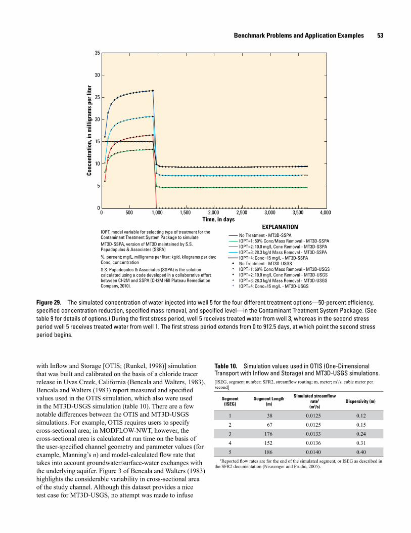
Benchmark Problems and Application Examples 53
Time, in days0 500 1,000 1,500 2,000 3,0002,500 4,0003,500
Conc
entr
atio
n, in
mill
igra
ms
per l
iter
0
5
10
15
20
25
30
35
No Treatment - MT3D-SSPAIOPT=1; 50% Conc/Mass Removal - MT3D-SSPAIOPT=2; 10.0 mg/L Conc Removal - MT3D-SSPAIOPT=3; 28.3 kg/d Mass Removal - MT3D-SSPAIOPT=4; Conc=15 mg/L - MT3D-SSPANo Treatment - MT3D-USGSIOPT=1; 50% Conc/Mass Removal - MT3D-USGSIOPT=2; 10.0 mg/L Conc Removal - MT3D-USGSIOPT=3; 28.3 kg/d Mass Removal - MT3D-USGSIOPT=4; Conc=15 mg/L - MT3D-USGS
EXPLANATIONIOPT, model variable for selecting type of treatment for the Contaminant Treatment System Package to simulateMT3D-SSPA, version of MT3D maintained by S.S. Papadopulos & Associates (SSPA)
%, percent; mg/L, milligrams per liter; kg/d, kilograms per day; Conc, concentration
S.S. Papadopulos & Associates (SSPA) is the solution calculated using a code developed in a collaborative effort between CH2M and SSPA (CH2M Hill Plateau Remediation Company, 2010).
Figure 29. The simulated concentration of water injected into well 5 for the four different treatment options—50-percent efficiency, specified concentration reduction, specified mass removal, and specified level—in the Contaminant Treatment System Package. (See table 9 for details of options.) During the first stress period, well 5 receives treated water from well 3, whereas in the second stress period well 5 receives treated water from well 1. The first stress period extends from 0 to 912.5 days, at which point the second stress period begins.
with Inflow and Storage [OTIS; (Runkel, 1998)] simulation that was built and calibrated on the basis of a chloride tracer release in Uvas Creek, California (Bencala and Walters, 1983). Bencala and Walters (1983) report measured and specified values used in the OTIS simulation, which also were used in the MT3D-USGS simulation (table 10). There are a few notable differences between the OTIS and MT3D-USGS simulations. For example, OTIS requires users to specify cross-sectional area; in MODFLOW-NWT, however, the cross-sectional area is calculated at run time on the basis of the user-specified channel geometry and parameter values (for example, Manning’s n) and model-calculated flow rate that takes into account groundwater/surface-water exchanges with the underlying aquifer. Figure 3 of Bencala and Walters (1983) highlights the considerable variability in cross-sectional area of the study channel. Although this dataset provides a nice test case for MT3D-USGS, no attempt was made to infuse
Table 10. Simulation values used in OTIS (One-Dimensional Transport with Inflow and Storage) and MT3D-USGS simulations. [ISEG, segment number; SFR2, streamflow routing; m, meter; m3/s, cubic meter per second]
Segment (ISEG)
Segment Length (m)
Simulated streamflow rate1
(m3/s)Dispersivity (m)
1 38 0.0125 0.12
2 67 0.0125 0.15
3 176 0.0133 0.24
4 152 0.0136 0.31
5 186 0.0140 0.401Reported flow rates are for the end of the simulated segment, or ISEG as described in
the SFR2 documentation (Niswonger and Prudic, 2005).
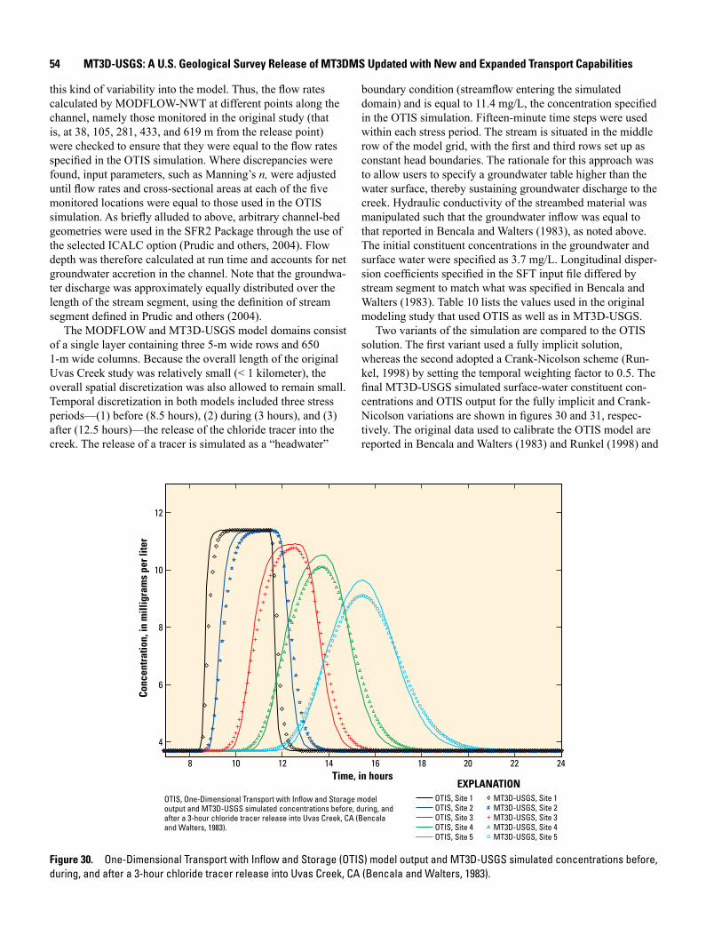
54 MT3D-USGS: A U.S. Geological Survey Release of MT3DMS Updated with New and Expanded Transport Capabilities
this kind of variability into the model. Thus, the flow rates calculated by MODFLOW-NWT at different points along the channel, namely those monitored in the original study (that is, at 38, 105, 281, 433, and 619 m from the release point) were checked to ensure that they were equal to the flow rates specified in the OTIS simulation. Where discrepancies were found, input parameters, such as Manning’s n, were adjusted until flow rates and cross-sectional areas at each of the five monitored locations were equal to those used in the OTIS simulation. As briefly alluded to above, arbitrary channel-bed geometries were used in the SFR2 Package through the use of the selected ICALC option (Prudic and others, 2004). Flow depth was therefore calculated at run time and accounts for net groundwater accretion in the channel. Note that the groundwa-ter discharge was approximately equally distributed over the length of the stream segment, using the definition of stream segment defined in Prudic and others (2004).
The MODFLOW and MT3D-USGS model domains consist of a single layer containing three 5-m wide rows and 650 1-m wide columns. Because the overall length of the original Uvas Creek study was relatively small (< 1 kilometer), the overall spatial discretization was also allowed to remain small. Temporal discretization in both models included three stress periods—(1) before (8.5 hours), (2) during (3 hours), and (3) after (12.5 hours)—the release of the chloride tracer into the creek. The release of a tracer is simulated as a “headwater”
boundary condition (streamflow entering the simulated domain) and is equal to 11.4 mg/L, the concentration specified in the OTIS simulation. Fifteen-minute time steps were used within each stress period. The stream is situated in the middle row of the model grid, with the first and third rows set up as constant head boundaries. The rationale for this approach was to allow users to specify a groundwater table higher than the water surface, thereby sustaining groundwater discharge to the creek. Hydraulic conductivity of the streambed material was manipulated such that the groundwater inflow was equal to that reported in Bencala and Walters (1983), as noted above. The initial constituent concentrations in the groundwater and surface water were specified as 3.7 mg/L. Longitudinal disper-sion coefficients specified in the SFT input file differed by stream segment to match what was specified in Bencala and Walters (1983). Table 10 lists the values used in the original modeling study that used OTIS as well as in MT3D-USGS.
Two variants of the simulation are compared to the OTIS solution. The first variant used a fully implicit solution, whereas the second adopted a Crank-Nicolson scheme (Run-kel, 1998) by setting the temporal weighting factor to 0.5. The final MT3D-USGS simulated surface-water constituent con-centrations and OTIS output for the fully implicit and Crank-Nicolson variations are shown in figures 30 and 31, respec-tively. The original data used to calibrate the OTIS model are reported in Bencala and Walters (1983) and Runkel (1998) and
Time, in hours
Conc
entr
atio
n, in
mill
igra
ms
per l
iter
8 10 12 14 16 18 20 22 24
4
6
8
10
12
OTIS, Site 1OTIS, Site 2OTIS, Site 3OTIS, Site 4OTIS, Site 5
EXPLANATIONMT3D-USGS, Site 1MT3D-USGS, Site 2MT3D-USGS, Site 3MT3D-USGS, Site 4MT3D-USGS, Site 5
OTIS, One-Dimensional Transport with Inflow and Storage model output and MT3D-USGS simulated concentrations before, during, and after a 3-hour chloride tracer release into Uvas Creek, CA (Bencala and Walters, 1983).
Figure 30. One-Dimensional Transport with Inflow and Storage (OTIS) model output and MT3D-USGS simulated concentrations before, during, and after a 3-hour chloride tracer release into Uvas Creek, CA (Bencala and Walters, 1983).

Benchmark Problems and Application Examples 55
are not replotted in figures 30 and 31. As stated previously, the purpose of this exercise was to verify the accuracy of the MT3D-USGS numerical simulation by comparing the results to output predicted by published codes.
Using the Crank-Nicoloson scheme yielded results that closely match those calculated by OTIS and first reported in Runkel (1998), which also uses a Crank-Nicolson scheme. Using a fully implicit scheme led to more dispersion in the final MT3D-USGS solution compared to the OTIS output.
LAK ExampleA simple lake transport problem is presented to verify the
accuracy of the LKT Package. This problem is described in Merritt and Konikow (2000) in the section “Test Simulation 1.” In this particular problem, a 5,000-day transient simulation period is divided into 100 time steps. Plan and profile views of the grid discretization are shown in figures 32A and 32B, respectively, with shaded cells showing the location of the lake within the model domain.
In this simple benchmark problem, initial groundwater concentrations are set equal to zero. Upon execution of the simulation, groundwater begins flowing into the lake as a result of a lake stage that is 50 ft below fixed groundwater
heads on the left edge of the model boundary. The initial constituent concentration in the lake is 100 mg/L. Thus, the discharge of “clean” groundwater to the lake dilutes the lake concentrations for the remainder of the simulation. Streams entering or exiting the lake are not simulated. Precipitation and evaporation rates of 0.0115 ft/d and 0.0103 ft/d, respectively, remain constant throughout the simulation and have associated concentrations equal to zero. Thus, the analytical solution for this problem is easy to calculate and is shown as the black line in figure 33. The simulated LKT concentrations, depicted as green color-filled circles in figure 33, demonstrate the accu-racy of MT3D-USGS.
As the lake fills, seepage from the lake to the surficial aquifer begins to occur at approximately 1,230 days into the simulation, when the lake stage rises sufficiently above the fixed head boundary along the right-hand edge of the model domain. Furthermore, after 3,000 simulation days, the amount of precipitation falling on the lake, which has a significantly expanded surface area by this point in the simulation, plus groundwater inflow to the lake is roughly balanced by the combination of evaporation and seepage losses to the surficial aquifer below the lake. Hence, even after the lake stage levels off, the lake constituent concentration continues to drop as solute is continually lost to the groundwater system through seepage occurring in parts of the lakebed, and is diluted by
Time, in hours
Conc
entr
atio
n, in
mill
igra
ms
per l
iter
8 10 12 14 16 18 20 22 24
4
6
8
10
12
OTIS, Site 1OTIS, Site 2OTIS, Site 3OTIS, Site 4OTIS, Site 5
EXPLANATIONMT3D-USGS, Site 1MT3D-USGS, Site 2MT3D-USGS, Site 3MT3D-USGS, Site 4MT3D-USGS, Site 5
OTIS, One-Dimensional Transport with Inflow and Storage
Figure 31. One-Dimensional Transport with Inflow and Storage (OTIS) model output and MT3D-USGS simulated concentrations using a Crank-Nicolson weighting factor of 0.5. MT3D-USGS using a weighting factor of 0.5, achieved a much better fit to the OTIS output than MT3D-USGS without the weighting factor at the five monitored locations.

56 MT3D-USGS: A U.S. Geological Survey Release of MT3DMS Updated with New and Expanded Transport Capabilities
13,000 feet
50 feet
13,000 feet
Layer
1
2
3
4
5
EXPLANATIONA
B
LAK cell
Figure 32. A 17-row by 17-column by 5-layer grid is used in the Lake Transport benchmark problem in A, plan and B, profile views. This problem first appeared in Merritt and Konikow (2000).
precipitation and by groundwater inflow occurring in other parts of the lakebed with zero (or very low) concentrations. The simulation maintains a good mass balance and verifies lake transport related calculations in the absence of lake–stream interaction.
GWT Example Test Simulation 2 of the SFR1 documentation (Prudic
and others, 2004), also appearing as Test Simulation 4 in the LAK Package documentation (Merritt and Konikow, 2000), was used to verify accurate simulation of stream–lake–aqui-fer interaction, where (1) groundwater to lake, (2) lake to groundwater, (3) stream to lake, (4) lake to stream, and (5) stream to groundwater exchanges are concurrently simulated in a groundwater/surface-water simulation. As stated in Mer-ritt and Konikow (2000), this problem is based on a sewage plume migrating through a sand and gravel aquifer on Cape Cod, Massachusetts (LeBlanc, 1984). Because observations of boron concentrations in both the sewage release and the
resulting plume were available, boron is the simulated species in this example. Though this simulation is not calibrated and is therefore not intended to be an accurate simulation of the contaminant migration, it nevertheless provides a good test case for groundwater/surface-water exchange and associated consequences on solute exchange between these two inte-grated systems. Migration of the contaminant is simulated over a 25-year period. Simulation values used in GWT and MT3D-USGS are provided in table 11.
At the beginning of the simulation, leaked sewage began migrating away from a spill site located near the top of the model domain; the leaked sewage migrated southward and intersected, or at least passed under, Ashumet Pond (Lake 1), the location of which is shown by yellow cells in figure 34. In the SFR1 presentation of the benchmark problem, creeks entering and exiting the lake are also simulated (fig. 34). Owing to the instantaneous mixing assumption in the lake, contaminated groundwater discharged to the lake is imme-diately available as a contaminant source to the underly-ing aquifer in locations where the lake is discharging to the groundwater system (note the higher isoconcentration lines in

Benchmark Problems and Application Examples 57
Time, in days0 5,0001,000 2,000 3,000 4,000
Conc
entr
atio
n, in
mill
igra
ms
per l
iter
0
20
40
60
80
100
1,000
2,000
3,000
4,000
5,000
6,000
7,000
Volu
me,
in a
cre
feet
Analytical solutionSimulated LKT concentrationSimulated LKT volume
EXPLANATION
LKT, Lake Transport Package
Figure 33. The analytical and simulated Lake Transport Package concentrations for the 5,000-day simulation. Groundwater discharge acts to dilute the lake concentrations. No other flows (for example, precipitation, evaporation, streamflow) enter or exit the lake. The red line, depicting total inundated lake volume, corresponds to the right y-axis.
Table 11. Parameter and property values used in the Groundwater Transport Package (GWT) benchmark problem used to further evaluate MT3D-USGS results when simulating aquifer-stream-lake (that is, SFT and LKT packages are active) transport processes simultaneously. [ft/d, feet per day; ft, feet; d, day; ft2/d, square feet per day; µg/L, micrograms per liter]
Model parameter Value
Horizontal hydraulic conductivity 250 ft/d
Vertical hydraulic conductivity 125 ft/d
Storage coefficient1 0
Aquifer thickness 120 ft
Porosity (ϕ; unitless) 0.30
Recharge rate 4.79 x 10⁻³ ft/d
Lakebed leakance 1 1/d
Streambed hydraulic conductivity 100 ft/d
Streambed thickness 1 ft
Longitudinal dispersivity 20 ft
Horizontal transverse dispersivity 2 ft
Vertical transverse dispersivity 0.20 ft
Diffusion coefficient 0 ft2/d
Initial concentration 0 μg/L
Source concentration 500 μg/L1Storage coefficient is set equal to 0 owing to the steady state nature of the simulation.
the vicinity where stream segment 2 exits the lake). Moreover, because stream segment 2 is a losing segment, contaminated lake water exiting the lake via the stream labeled “2” (fig. 34) will contaminate the downgradient areas of the aquifer much faster than groundwater contaminant transport alone would predict. More generally, contaminant discharging to a surface-water system, albeit at low levels, acts as a short circuit allow-ing the contaminant to move rapidly through a modeled sys-tem. Thus, capabilities for simulating both the aquifer and the surface-water system provide a powerful tool for simulating contaminant transport in connected stream–aquifer systems.
UZT Benchmark Problems
Three sets of one-dimensional analytical solutions reported in Vanderborght and others (2005) are used to confirm the accuracy of MT3D-USGS as applied to variably saturated con-ditions. The first benchmark problem includes only variations in dispersivity; the reaction package is inactive. The second and third benchmark problems demonstrate that the UZT Package works properly when reactions (in this case, sorption) are simulated in the unsaturated zone. The second problem can be solved analytically; it incorporates nonlinear sorption when the equilibrium assumption is appropriate. Sorption

58 MT3D-USGS: A U.S. Geological Survey Release of MT3DMS Updated with New and Expanded Transport Capabilities
Inactive cells
Constant head at 50.0 feet, and concentration in fluid source is zero
Constant head from 50.10 to 50.15 feet, and constant concentration in fluid source of 500 micrograms per liter
Constant head at 28.0 feet
Lake 1
Lake 2
Stream and segment number
Isoconcentration contour lines as calcuated by the software GWT and number, in grams per liter
Isoconcentration contour lines as calculated by MT3D-USGS and number, in grams per liter
No-flow boundary (frame around cell grid)
Layer 1 Layer 3Columns
Layer 5 Columns
Columns
1
10
20
30
36
Row
s
1
10
20
30
36
Row
s
1 5 10 15 20 23 1 5 10 15 20 23
10
20
30
36
Row
s
1 5 10 15 20 23
1
EXPLANATION
4
4
2
3
1
4
23
1
4
23
1250
2525
100
10
10
25
1
1
250
250
250
25
25
25
2525
25
100
100
100
100
100
10
1010
1010
10
1
1
1
1
11
25
25
1
1
10
10
10
1010
1
1
25
25
100
100
250
1
1
100
GWT data are from Merritt and Konikow (2000) and Prudic and others (2004)
Figure 34. Boron isoconcentration contours for A, layer 1, B, layer 3, and C, layer 5 in a connected stream-aquifer system after 25 years for the Groundwater Transport Package and MT3D-USGS.

Benchmark Problems and Application Examples 59
occurs when dissolved phase mass is converted to solid phase mass by fixing onto the porous medium through which the fluid is traveling. When the transfer of mass between the dis-solved and solid phases happens sufficiently fast relative to groundwater velocity, the equilibrium-controlled assumption is valid (Zheng and Bennett, 2002). In conditions where the equilibrium assumption is invalid (that is, sorption and desorp-tion processes do not occur sufficiently fast relative to the time in which solute and porous media are in contact with one another), MT3D-USGS, as with MT3D, can simulate nonequi-librium controlled reactions. This type of reaction is tested by the third benchmark problem of this section solved analyti-cally and with MT3D-USGS.
Variations in DispersivityThe first UZT benchmark problem explores the perfor-
mance of the UZT Package under two different dispersivi-ties separated by two orders of magnitude. A steady-flow, one-dimensional model spanning 200 centimeters (cm) was created for comparison with the analytical benchmark. Vertical discretization is 1 cm; other model parameters are listed in table 12 and are specified on the basis of the analyti-cal solution described by Vanderborght and others (2005). Simulated output for dispersivities (αL) of 0.1 and 10 cm are compared to the respective analytical solutions reported in Vanderborght and others (2005). Peclet numbers (Δx/αL) for the 0.1- and 10-cm dispersivity benchmark models are 10 and 0.1, respectively. Zheng and Bennett (2002) recommend grid Peclet numbers be kept below 2; otherwise, artificial numeri-cal oscillations may result from sharp concentration fronts. Because the benchmark problem with αL equal to 0.1 cm results in a Peclet number of 10, the model was run twice. In the first simulation, the advection and dispersion terms are solved using the implicit finite-difference method. The second simulation invoked the TVD scheme and the implicit finite-difference method to solve the advection term. This was done
to overcome numerical difficulties associated with the high Peclet number. As with the first variant of this benchmark simulation, the dispersion term is solved using the implicit finite-difference method.
Results for the simulation with αL equal to 0.1 cm are shown in figure 35. As expected, the simulated concentrations without the use of the TVD scheme led to artificial oscilla-tions. As a result, negative concentrations are a part of the final solution (see figure 35A inset). With the TVD option activated, the MT3D-USGS solution achieved an excellent match to the analytical solution.
For the simulation with αL equal to 10.0 cm (Peclet num-ber equal to 0.1), the simulated concentration matched the analytical solution over most of the 200-cm profile. Concen-trations are slightly over predicted near the bottom boundary (190–200 cm), which may be due to the proximity of the model boundary, which is 10 cm (or 1 αL) beyond the interval over which the analytical solution was calculated. Despite the misfit near the boundary of the simulated domain, there is good agreement between the analytical and simulated concen-trations for the simulation with αL equal to 10 cm.
Nonlinear Equilibrium SorptionAn analytical solution for non-linear equilibrium con-
trolled reaction under variably saturated conditions described in Vanderborght and others (2005) is used to verify MT3D-USGS results when both the UZT and RCT Packages are active. Model parameter values and boundary conditions that are congruent with the specified analytical solution values are listed in table 13. The Freundlich isotherm, which assumes that the aquifer material has infinite storage capacity (Zheng and Bennett, 2002), was used to simulate retardation in this problem. Because the shape of the downward advancing concentration front remains constant with time (Vanderborght and others, 2005), the analytical solution was provided for transformed depth coordinates, the equation for which is given in Vanderborght and others (2005). In addition to the analyti-cal solution, a variably saturated two-dimensional transport [VS2DT; (Healy, 1990; Lappala and others, 1987)] solution was calculated to show the advance of the concentration front with time (20, 40, and 60 days) using untransformed coordi-nates. The MT3D-USGS solution matches well the analyti-cal benchmark solution (fig. 36A) and the VS2DT solution (fig. 36B).
Table 12. Parameter values for the Unsaturated-Zone Flow and Transport packages (UZF and UZT, respectively) in a benchmark model used for testing two dispersivities. [mg/L, milligrams per liter; cm/d, centimeters per day; cm, centimeters; >, greater than; <, less than; ≤, less than or equal to]
Model parameter Value
Initial water content 0.378639
Initial concentration 0.00 mg/L
Infiltrating flux 5 cm/d
Vertical hydraulic conductivity 50.0 cm/d
Saturated water content 0.43
Residual water content 0.08
Dispersivity (αL) 0.1, 10 cm
Concentration of infiltrating water
0 < t ≤ 1 day 100 mg/L
t > 1 day 0 mg/L
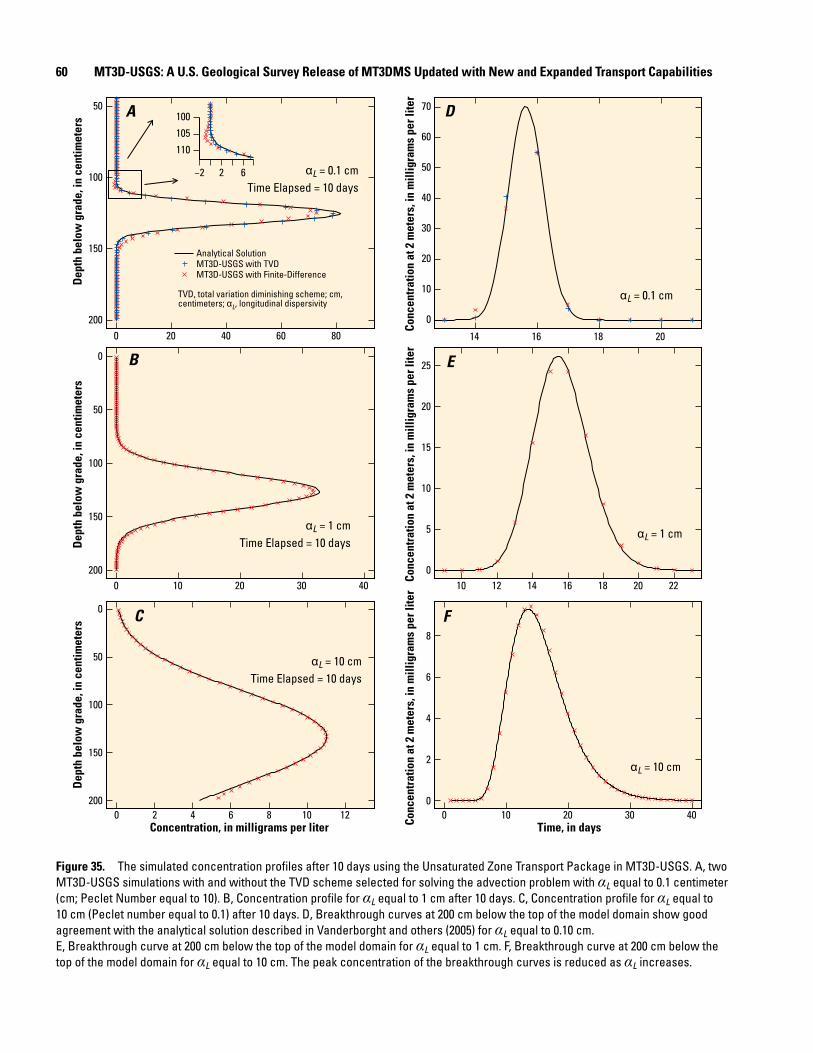
60 MT3D-USGS: A U.S. Geological Survey Release of MT3DMS Updated with New and Expanded Transport CapabilitiesD
epth
bel
ow g
rade
, in
cent
imet
ers
Dep
th b
elow
gra
de, i
n ce
ntim
eter
sD
epth
bel
ow g
rade
, in
cent
imet
ers
200
150
100
50
200
150
100
50
0
200
150
100
50
0
0 20 40 60 80
A D
0
10
20
30
40
50
60
70
14 16 18 20
E
0
5
10
15
20
25
10 20 30 40 10 12 14 16 18 20 22
B
C F
0 2 4 6 8 10 12 0 10 20 30 40Time, in daysConcentration, in milligrams per liter
Time Elapsed = 10 days
Conc
entr
atio
n at
2 m
eter
s, in
mill
igra
ms
per l
iter
Conc
entr
atio
n at
2 m
eter
s, in
mill
igra
ms
per l
iter
Conc
entr
atio
n at
2 m
eter
s, in
mill
igra
ms
per l
iter
0
0
2
4
6
8
Time Elapsed = 10 days
Time Elapsed = 10 days
αL = 10 cm
αL = 0.1 cm
110
105
100
−2 2 6
Analytical SolutionMT3D-USGS with TVDMT3D-USGS with Finite-Difference
TVD, total variation diminishing scheme; cm, centimeters; αL, longitudinal dispersivity
αL = 10 cm
αL = 1 cmαL = 1 cm
αL = 0.1 cm
Figure 35. The simulated concentration profiles after 10 days using the Unsaturated Zone Transport Package in MT3D-USGS. A, two MT3D-USGS simulations with and without the TVD scheme selected for solving the advection problem with αL equal to 0.1 centimeter (cm; Peclet Number equal to 10). B, Concentration profile for αL equal to 1 cm after 10 days. C, Concentration profile for αL equal to 10 cm (Peclet number equal to 0.1) after 10 days. D, Breakthrough curves at 200 cm below the top of the model domain show good agreement with the analytical solution described in Vanderborght and others (2005) for αL equal to 0.10 cm. E, Breakthrough curve at 200 cm below the top of the model domain for αL equal to 1 cm. F, Breakthrough curve at 200 cm below the top of the model domain for αL equal to 10 cm. The peak concentration of the breakthrough curves is reduced as αL increases.

Benchmark Problems and Application Examples 61
Table 13. Parameter values for the flow and transport bench-mark model used for testing nonlinear equilibrium controlled sorption in the unsaturated zone. [mg/L, milligrams per liter; cm/d, centimeters per day; cm, centimeters; g/mL, grams per milliliter; mg/mL, milligrams per milliliter]
Model parameter Value
Initial water content 0.40
Initial concentration 0.00 mg/L
Infiltrating flux 2 cm/d
Vertical hydraulic conductivity 3.0 cm/d
Saturated water content 0.43
Residual water content 0.08
Dispersivity (αL) 1.0 cm
Bulk density (ρb) 1.0 g/mL
Freundlich isotherm parameter1 (a) 2/3
Partitioning coefficient1 (Kf) 1 mL/(g/mga-1)
Concentration of infiltrating water (t > 0) 10 mg/mL1The parameters ρb and a are used to calculate the retardation coefficient, R, for the
Freundlich isotherm expressed in the form R = 1 +(—ρb
θ )aKƒCa−1.
Nonequilibrium SorptionSome field conditions may render the equilibrium assump-
tion inappropriate. In this situation, reactions (that is, sorption and desorption) can be simulated using first-order revers-ible kinetic reactions. As with the previous two examples, an analytical benchmark problem first appearing in Vander-borght and others (2005) is used to confirm that MT3D-USGS accurately models dissolved and sorbed concentrations when retardation (that is, sorption and desorption) is rate limited (nonequilibrium). Model parameter values used in this simula-tion are listed in table 14. Infiltration is steady and equal to the vertical hydraulic conductivity. Constant head boundaries were used to fix the water table below the upper 10 cm of the model domain, the region of the published analytical solu-tion (Vanderborght and others, 2005). After the equivalent of 20 pore volumes (200 1/hr) passed through the upper 10 cm of the model domain, inflow was interrupted long enough to allow the dissolved and sorbed concentration to equilibrate. Naturally occurring gravity drainage was prevented by replac-ing the 480-hour stop-flow period flux terms with zeroes in the FTL file. After the stop-flow period, infiltration and subse-quent drainage resumed pre-stop-flow rates.
The dissolved and sorbed concentration profiles closely match the analytical solution calculated for the moment preceding the stop-flow period (that is, 200 hour; fig. 37A). Figure 37B shows the concentration breakthrough curve with pore volumes marking elapsed time in order to easily account for the stop-flow period. A slight bump in the concentration at 100 mm below grade when flow resumes (that is, 20 pore vol-umes) results from the release of sorbed mass during the stop-flow period that subsequently flows past the observation depth. Good agreement between MT3D-USGS and the analytical solution is achieved throughout the simulated period.
Table 14. Parameter values for the flow and transport benchmark model used for testing the nonequilibrium controlled sorption problem with flow terms calculated by the Unsaturated Zone Flow (UZF1) Package. [mg/L, milligrams per liter; cm/hr, centimeters per hour; cm, centimeters; g/mL, grams per milliliter; mL/g, milliliter per gram; mg/mL, milligrams per milliliter; hr, hour(s); >, greater than; <, less than; ≤, less than or equal to; t, time; C, concentration; C—, sorbed concentration]
Model parameter Value
Initial water content 0.50
Initial concentration 0.00 mg/L
Infiltrating flux 0.5 cm/hr
Vertical hydraulic conductivity 0.5 cm/hr
Saturated water content 0.50
Residual water content 0.15
Dispersivity (αL) 1.0 cm
Bulk density (ρb) 1.0 g/mL
1st order mass transfer rate1 (β) 0.10 1/hr
Partitioning coefficient1 (Kd) 10. mL/g
Concentration of infiltrating water
0 < t ≤ 1 day 100,000 mg/mL
t > 1 day 0 mg/mL1The parameters Kd and β are used to calculate non-equilibrium sorption using the
equation β∂∂ρb Kd
CCtC = where C— is the concentration of the sorbed phase. The mass
transfer coefficient αs used in equation 12 of Vanderborght and others (2005) and equal to 0.01 1/hr in the original benchmark problem differs from β used in MT3D-USGS by a factor of ρbKd (Zheng and Wang, 1999).
Regional Scale UZT ApplicationAlthough helpful for demonstrating accuracy, the three
previous UZT example applications rely on one-dimensional simulations. Here, the problem that first appeared in Keating and Zyvoloski (2009) and used in the “Routing Mass through Dry Cells” section is modified by adding unsaturated-zone transport in the cells above the perched aquifer. This applica-tion uses the parameter values listed in table 3 plus the new unsaturated-zone parameters listed in table 15. Figures 38A, 38B, and 38C show snapshots of the spread of the contami-nation through the unsaturated and saturated zones of the regional aquifer at 730, 2,500, and 9,000 days, respectively. Alterations in the concentration breakthrough curves result-ing from explicit simulation of unsaturated-zone transport are shown in figures 39A and 39B, where lengthy delays (>> 1,000 days) in the peak breakthrough concentrations are noted. The locations of the observations points are given in figures 11A and 38A.
This example highlights a current limitation in both the UZF1 and UZT Packages; unsaturated-zone transport is simulated only between the area where infiltration is speci-fied in the flow model (commonly land surface) and the first encounter with a saturated cell. Subsequent unsaturated-zone flow and transport, for example where the perched aquifer spills over the edge of the aquitard, is not supported by the UZF1 flow package and, therefore, cannot be simulated in this
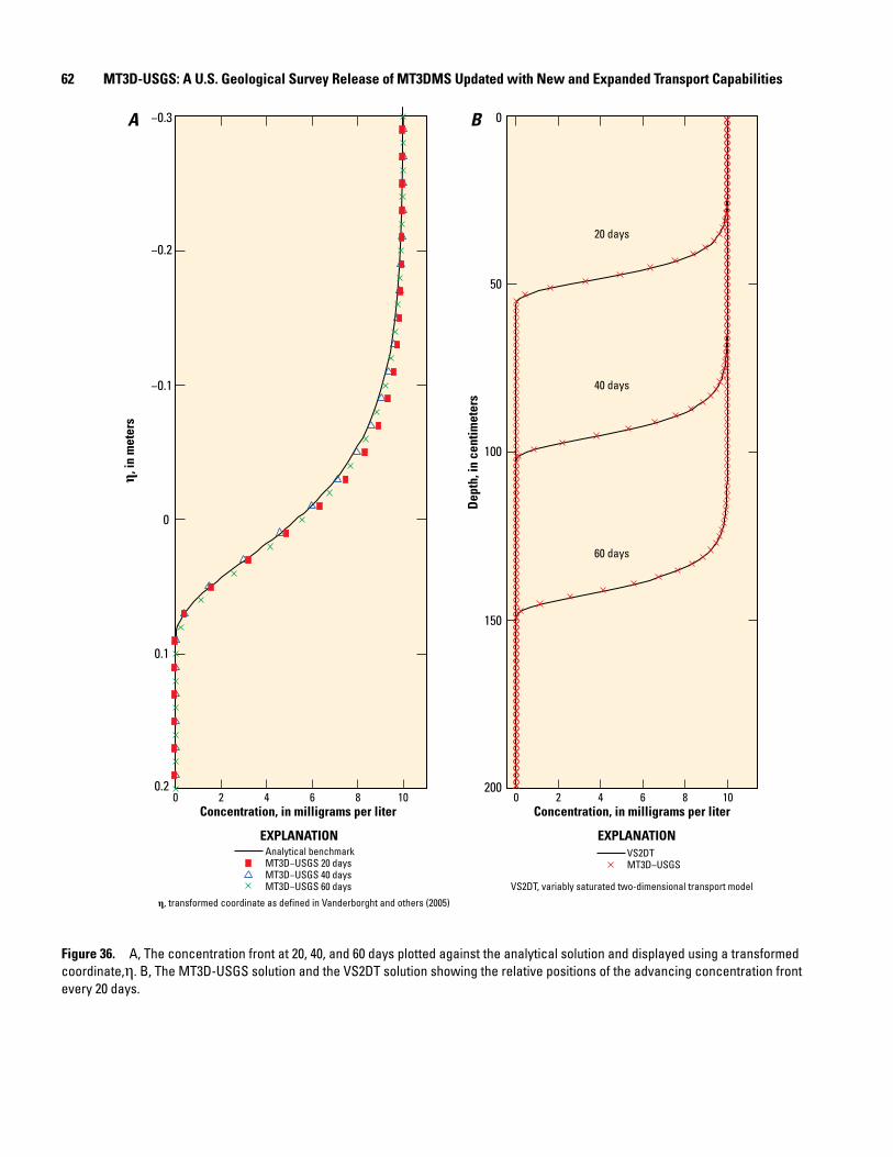
62 MT3D-USGS: A U.S. Geological Survey Release of MT3DMS Updated with New and Expanded Transport Capabilities
Dep
th, i
n ce
ntim
eter
s
η, in
met
ers
A B
Concentration, in milligrams per liter Concentration, in milligrams per liter0 2 4 6 8 10 0 2 4 6 8 10
200
150
100
50
0
0.2
0.1
−0.1
−0.2
−0.3
0
20 days
40 days
60 days
Analytical benchmarkMT3D−USGS 20 daysMT3D−USGS 40 daysMT3D−USGS 60 days
VS2DTMT3D−USGS
EXPLANATION EXPLANATION
VS2DT, variably saturated two-dimensional transport model
η, transformed coordinate as defined in Vanderborght and others (2005)
Figure 36. A, The concentration front at 20, 40, and 60 days plotted against the analytical solution and displayed using a transformed coordinate,η. B, The MT3D-USGS solution and the VS2DT solution showing the relative positions of the advancing concentration front every 20 days.

Benchmark Problems and Application Examples 63D
epth
, in
mill
imet
ers
A B
Concentration, in milligrams per liter
Conc
entr
atio
n, in
mill
igra
ms
per l
iter
0 10 20 30 40 500 5 10 15 20Pore Volumes (T)
100
80
60
40
20
0
0
5
10
15
20
25
30
Analytical dissolved concentrationAnalytical sorbed concentrationMT3D−USGS dissolved concentrationMT3D−USGS sorbed concentration
1.5
1.6
1.7
1.8
1.9
2.0
2.1
0
10
20
30
40
0 1 2 20 21 22
Analytical benchmarkMT3D−USGS
EXPLANATION EXPLANATION
T, time which in this example is quantified by the passage of pore volumes
Figure 37. A, Profile of dissolved and sorbed constituent concentrations in the upper 100 millimeters of the model domain 200 hours after the initial injection of contaminated water. Infiltrating water was assigned a concentration of 100,000 milligrams per liter for a duration of 0.01 hour (36 seconds) and 0.0 afterward. B, Breakthrough concentrations at 100-millimeter depth. The bump in concentration at 20 pore volumes follows the stop-flow period and is due to the release of sorbed mass to the dissolved phase during the stop-flow period.

64 MT3D-USGS: A U.S. Geological Survey Release of MT3DMS Updated with New and Expanded Transport Capabilities
Table 15. Unsaturated zone parameter values for a two-dimensional (2D) benchmark model simulating transport through the unsaturated zone in a perched aquifer simulation. [mg/L, milligrams per liter; ft/d, feet per day; ft, feet; t, time; >, greater than; <, less than; ≤, less than or equal to]
Model parameter Value
Initial water content 0.254
Initial concentration 0.0 mg/L
Infiltrating flux 0.072 ft/d
Vertical hydraulic conductivity of unsaturated zone 0.85 ft/d
Saturated water content 0.3
Residual water content 0.2
Brooks-Corey exponent (ε) 4
Dispersivity (αL) 1 ft
Concentration in infiltrating water
0 < t ≤ 730 day 1 mg/L
t > 730 day 0 mg/L
Concentration, in milligrams per liter0.01 0.10 0.50 0.90 0.99
2,000 4,000 6,000 8,000 10,0000
2,000
1,500
1,000
500
0
2,000
1,500
1,000
500
02,000
1,500
1,000
500
0
EXPLANATION
Saturated zone
Observation point
A
B
C
See Figure 39A
See Figure 39B
Aquitard
Aquitard
Aquitard
Distance, in meters
Elev
atio
n, in
met
ers
730 days
2,500 days
9,000 days
Figure 38. Progression of a hypothetical plume that originates from infiltration occurring at land surface. A, Solute travels downward under variably saturated conditions toward the perched aquifer and B, eventually reaches the perched aquifer, spreads throughout it, and begins spilling over the sides of the aquitard. C, After arrival in the lower part of the regional aquifer, the plume migrates toward the right model boundary.
release of MT3D-USGS. However, use of the DRYCELL key-word option ensures that the mass spilling over the sides of the aquitard is reintroduced to the lower regional aquifer; without the use of this option, mass would accumulate in the perched aquifer owing to dry cells blocking its downward migration. As previously described, transport occurs instantaneously through cells separating the perched and regional aquifers.

Benchmark Problems and Application Examples 65
0
0.1
0.2
0.3
0.4
0.5
0.6
0.7
0.8
Conc
entr
atio
n, in
mill
igra
ms
per l
iter
0 1,000 2,000 3,000 4,000 5,000 6,000 7,000 8,000Time, in days
Conc
entr
atio
n, in
mill
igra
ms
per l
iter
Time, in days
MT3D-USGS, UZT inactiveMT3D-USGS, UZT active
0
0.05
0.10
0.15
0.20
0 5,000 10,000 15,000 20,000 25,000 30,000 35,000 40,000
A
B
EXPLANATION
UZT, Unsaturated Zone Transport Package
Figure 39. Concentration breakthrough curves in the perched aquifer problem with and without simulating transport in the unsaturated zone above the perched aquifer. Breakthrough curves are for two points located A, within the lower regional aquifer below the left end of the aquitard and B, within the lower regional aquifer close to where groundwater flows out of the MODFLOW and MT3D-USGS simulations. Location of the observations points are shown in figure 38A.

66 MT3D-USGS: A U.S. Geological Survey Release of MT3DMS Updated with New and Expanded Transport Capabilities
SummaryThis report describes modifications made to the popular
MT3DMS v5.3 program, resulting in a new version of MT3D called MT3D-USGS. As new packages have been added to MODFLOW over the years, solute transport support for the flow terms calculated within these packages (for example, UZF1) was needed. Thus, nearly all of the enhancements to existing MT3DMS packages, as well as the new packages, are a result of practical application problems using recent versions of MODFLOW.
MT3D-USGS is backward compatible, making it pos-sible to run existing MT3DMS models within MT3D-USGS. Programmers will note that MT3D-USGS source code was rewritten such that the modules programming approach, described in the MODFLOW-2005 documentation, is now adopted. Several enhancements to existing MT3DMS pack-ages have been described, most notably the ability to simulate transport through dry cells for use with MODFLOW-NWT simulations and inter-species reactions within the RCT pack-age. Several new packages support the simulation of solute transport in lakes, streams, and the unsaturated zone, and are referred to as the LKT, SFT, and UZT Packages, respectively. These new packages not only route solutes through their respective domains, but account for solute exchange with the groundwater system. In addition, solute exchange among these packages, including streams contributing dissolved constitu-ents to lakes (SFT to LKT exchange), contaminated lake outflows into streams (LKT to SFT exchange), and overland runoff from non-infiltrated water and groundwater discharge into either streams or lakes (UZT to SFT and (or) UZT to LKT exchange), is supported. A fourth package available with MT3D-USGS, referred to as the CTS Package, facili-tates simulation of pump-and-treat systems for groundwater remediation. The features and capabilities of the MT3D-USGS program are demonstrated using several example problems.
References Cited
Alexander, M., 1994, Biodegradation and bioremediation: San Diego, Calif., Academic Press, 302 p.
Alvarez, P.J., and Illman, W.A., 2006, Bioremediation and natural attenuation: Process fundamentals and math-ematical models: Hoboken, N.J., John Wiley & Sons, Inc., 609 p.
Bencala, K.E., and Walters, R.A., 1983, Simulation of solute transport in a mountain pool-and-riffle stream: A Transient Storage Model: Water Resources Research, v. 19, no. 3, p. 718–724.
Carey, G.R., Van Geel, P.J., and Murphy, J.R., 1999, BioRe-dox-MT3DMS Version 2.0: A coupled biodegrada-tion-redox model for simulating natural and enhanced bioremediation of organic pollutants—User’s guide: Waterloo, Ontario, Canada: Conestoga-Rovers & Associates.
CH2M Hill Plateau Remediation Company, 2010, MOD-FLOW and Related Codes Software Management Plan: Report prepared under contract no. 00258 Rev 2 for the U.S. Department of Energy, Richland, Washington.
Charbeneau, R.J., Weaver, J.W., and Lien, B.K., 1995, The hydrocarbon spill screening model (HSSM), Vol-ume 2: Theoretical background and source codes: EPA/600/R-94/039b, Robert S. Kerr Environmental Research Laboratory, U.S. Environmental Protection Agency, Ada, Oklahoma.
Clement, T.P., 1997, A modular computer code for simulat-ing reactive multispecies transport in 3-dimensional groundwater systems: Technical Report PNNL-SA-11720, Pacific Northwest National Laboratory, Richland, Wash.
Guerin, M., and Zheng, C., 1998, GMT3D—Coupling multicomponent, three-dimensional transport with geochemistry, in, E.P., Zheng, C., and Hill, M.C., eds., Proceedings of the MODFLOW'98 International Conference, Colorado, Colorado School of Mines.
Halford, K.J., and Hanson, R.T., 2002, MODFLOW-2000, User guide for the drawdown-limited, Multi-Node Well (MNW) Package for the U.S. Geological Survey’s modular three-dimensional ground-water flow model, versions MODFLOW-96 and MOD-FLOW-2000: U.S. Geological Survey Open-File Report 02–293, p. 39.
Harbaugh, A.W., 2005, MODFLOW-2005: The U.S. Geo-logical Survey Modular Ground-water Model–the Ground-water Flow Process: U.S. Geological Survey Techniques and Methods 6-A16, p. 253.
Harbaugh, A.W., Banta, E.R., Hill, M.C., and McDonald, M.G., 2000, MODFLOW-2000, the U.S. Geological Survey modular ground-water model: User guide to modularization concepts and the ground-water flow process: U.S. Geological Survey Open-File Report 00–92 p. 121.
Harman, C., Rao, P., Basu, N., McGrath, G., Kumar, P., and Sivapalan, M., 2011, Climate, soil, and vegetation controls on the temporal variability of vadose zone transport: Water Resources Research, v. 47, no. 1, p. W00J13.

References Cited 67
Healy, R.W., 1990, Simulation of solute transport in variably saturated porous media with supplemental informa-tion on modification to the U.S. Geological Survey’s computer program VS2D: U.S. Geological Survey Water-Resources Investigations Report 90–4025, 130 p.
Hughes, J.D., Langevin, C.D., Chartier, K.L., and White, J.T., 2012, Documentation of the Surface-Water Routing (SWR1) Process for Modeling Surface-Water Flow with the U.S. Geological Survey Modular Ground-Water Model (MODFLOW-2005): U.S. Geological Survey Techniques and Methods book 6, chap. 40 (version 1.0), p. 113.
Keating, E., and Zyvoloski, G., 2009, A stable and efficient numerical algorithm for unconfined aquifer analysis: Groundwater, v. 47, no. 4, p. 569–579.
Konikow, L.F., Goode, D.J., and Hornberger, G.Z., 1996, A three-dimensional method-of-characteristics solute-transport model (MOC3D): U.S. Geological Survey Water-Resources Investigations Report 96–4267, p. 87.
Konikow, L.F., and Hornberger, G.Z., 2006, Modeling effects of multinode wells on solute transport: Ground Water, v. 44, no. 5, p. 648–660.
Konikow, L.F., Hornberger, G.Z., Halford, K.J., and Hanson, R.T., 2009, Revised Multi-Node Well (MNW2) Pack-age for MODFLOW ground-water flow model: U.S. Geological Survey Techniques and Methods 6–A30, p. 67.
Langevin, C.D., Thorne, D.T., Dausman, A.M., Sukop, M.C., and Guo, W., 2008, SEAWAT version 4: A computer program for simulation of Multi-Species Solute and Heat Transport: U.S. Geological Survey Techniques and Methods Book 6–A22, 39 p.
Lappala, E.G., Healy, R.W., and Weeks, E.P., 1987, Documen-tation of computer program VS2D to solve the equa-tions of fluid flow in variably saturated porous media: U.S. Geological Survey Water-Resources Investiga-tions Report 83–4238, p. 193.
LeBlanc, D.R., 1984, Sewage plume in a sand and gravel aquifer, Cape Cod, Massachusetts: U.S. Geological Survey Water-Supply Paper 2218, p. 28.
Lu, G., Clement, T.P., Zheng, C., and Wiedemeier, T.H., 1999, Natural attenuation of BTEX compounds: Model development and field-scale application: Ground Water, v. 37, no. 5, p. 707–717.
McGrath, G., Hinz, C., and Sivapalan, M., 2008a, Modelling the impact of within storm variability of rainfall on the loading of solutes to preferential flow pathways: European Journal of Soil Science, v. 59, no. 1, p. 24–33.
McGrath, G.S., Hinz, C., and Sivapalan, M., 2008b, Model-ing the effect of rainfall intermittency on the vari-ability of solute persistence at the soil surface: Water Resources Research, v. 44, no. 9, p. W09432, doi:09410.01029/02007WR006652.
Merritt, M.L., and Konikow, L.F., 2000, Documentation of a computer program to simulate lake-aquifer inter-action using the MODFLOW ground-water flow model and the MOC3D solute-transport model: U.S. Geological Survey Water-Resources Investigations Report 00–4167, 146 p.
Monod, J., 1949, The growth of bacterial cultures: Annual Reviews in Microbiology, v. 3, p. 371–394.
Morway, E.D., Niswonger, R.G., Langevin, C.D., Bailey, R.T., and Healy, R.W., 2013, Modeling variably saturated subsurface solute transport with MODFLOW-UZF and MT3DMS: Groundwater, v. 51, no. 2, p. 237–251.
Neville, C.J., and Tonkin, M.J., 2004, Modeling multiaquifer wells with MODFLOW: Ground Water, v. 42, no. 6, p. 910–919.
Neville, C.J., and Zhang, J., 2010, Benchmark analysis of sol-ute transport with multiaquifer wells: Ground Water, v. 48, no. 6, p. 884–891.
Niswonger, R., Panday, S., and Ibaraki, M., 2011, MOD-FLOW-NWT, A Newton formulation for MOD-FLOW-2005: U.S. Geological Survey Techniques and Methods 6–A37, 44 p.
Niswonger, R.G., Prudic, D.E., and Regan, R.S., 2006, Docu-mentation of the Unsaturated-Zone Flow (UZF1) Package for modeling unsaturated flow between the land surface and the water table with MOD-FLOW-2005: U.S. Geological Survey Techniques and Methods 6–A19, 62 p.
Panday, S., Langevin, C.D., Niswonger, R.G., Ibaraki, M., and Hughes, J.D., 2013, MODFLOW–USG version 1: An unstructured grid version of MODFLOW for simulat-ing groundwater flow and tightly coupled processes using a control volume finite-difference formulation: U.S. Geological Survey Techniques and Methods, book 6–A45, 66 p.
68 MT3D-USGS: A U.S. Geological Survey Release of MT3DMS Updated with New and Expanded Transport Capabilities
Parkhurst, D.L., and Appelo, C., 1999, User’s guide to PHREEQC (Version 2): A computer program for speciation, batch-reaction, one-dimensional transport, and inverse geochemical calculations: U.S. Geologi-cal Survey Water-Resources Investigations Report 99–4259, 312 p.
Prommer, H., Barry, D.A., and Zheng, C., 2003, MODFLOW/MT3DMS Based Reactive Multicomponent Transport Modeling: Ground Water, v. 41, no. 2, p. 247–257.
Prudic, D.E., Konikow, L.F., and Banta, E.R., 2004, A new Streamflow-Routing (SFR1) Package to simulate stream-aquifer interaction with MODFLOW-2000: U.S. Geological Survey Open-File Report 2004–1042, 96 p.
Richards, L.A., 1931, Capillary conduction of liquids through porous mediums: Journal of Applied Physics, v. 1, no. 5, p. 318–333.
Rifai, H.S., Newell, C.J., Gonzales, J.R., and Wilson, J.T., 2000, Modeling natural attenuation of fuels with BIOPLUME III: Journal of Environmental Engineer-ing, v. 126, no. 5, p. 428–438.
Ross, P.J., 1990, Efficient numerical methods for infiltration using Richards’ equation: Water Resources Research, v. 26, no. 2, p. 279–290.
Runkel, R.L., 1998, One-Dimensional Transport with Inflow and Storage (OTIS): A Solute Transport Model for Streams and Rivers: U.S. Geological Survey Water-Resources Investigations Report 98–4018, 73 p.
Schlesinger, W.H., 1997, Biogeochemistry: An analysis of global change (2d ed.): San Diego, Calif., Academic Press.
Smith, R., and Hebbert, R., 1983, Mathematical simulation of interdependent surface and subsurface hydrologic processes: Water Resources Research, v. 19, no. 4, p. 987–1001.
Smith, R.E., 1983, Approximate sediment water movement by kinematic characteristics: Soil Science Socity of America Journal, v. 47, p. 3–8.
Struthers, I., Hinz, C., and Sivapalan, M., 2006, A multiple wetting front gravitational infiltration and redistri-bution model for water balance applications: Water Resources Research, v. 42, no. 6, p. W06406.
Van Dam, J.C., and Feddes, R.A., 2000, Numerical simulation of infiltration, evaporation and shallow groundwater levels with the Richards equation: Journal of Hydrol-ogy, v. 233, no. 1–4, p. 72–85.
Vanderborght, J., Kasteel, R., Herbst, M., Javaux, M., Thiery, D., Vanclooster, M., Mouvet, C., and Vereecken, H., 2005, A set of analytical benchmarks to test numeri-cal models of flow and transport in soils: Vadose Zone Journal, v. 4, no. 1, p. 206–221.
Waddill, D.W., and Widdowson, M.A., 1998, SEAM3D: A numerical model for three-dimensional solute trans-port and sequential electron acceptor-based bioreme-diation in groundwater: Technical Report, Virginia Tech., Blacksburg, Virginia, accessed June 14, 2015, at ftp://weppi.gsf.fi/mirrors/gms/gms/gms3.0/docs/SEAM3Dv2.pdf.
Weaver, J.W., Charbeneau, R.J., Tauxe, J.D., Lien, B.K., and Provost, J.B., 1994, The hydrocarbon spill screening model (HSSM) Volume 1: User’s guide: EPA/600/R-94/039a, Robert S. Kerr Environmental Research Laboratory, U.S. Environmental Protection Agency, Ada, Oklahoma, accessed June 14, 2015, at http://sdi.odu.edu/mbin/hssm/windows/hssm1.pdf.
Wiedemeier, T.H., Rifai, H.S., Newell, C.J., and Wilson, J.T., 1999, Natural attenuation of fuels and chlorinated solvents in the subsurface: New York, John Wiley & Sons, Inc.
Wu, M.Z., Post, V.E.A., Salmon, S.U., Morway, E.D., and Prommer, 2015, PHT3D-UZF: A reactive transport model for variably-saturated porous media: Ground-water. doi: 10.1111/gwat.12318, accessed June 14, 2016, at http://onlinelibrary.wiley.com/doi/10.1111/gwat.12318/full.
Yeh, G., and Tripathi, V., 1989, A critical evaluation of recent developments in hydrogeochemical transport mod-els of reactive multichemical components: Water Resources Research, v. 25, no. 1, p. 93–108.
Zheng, C., 1990, MT3D, A modular three-dimensional trans-port model for simulation of advection, dispersion and chemical reactions of contaminants in groundwa-ter systems: Report to the U.S. Environmental Protec-tion Agency, Robert S. Kerr Environmental Research Laboratory, Ada, Oklahoma.
Zheng, C., 1996, MT3D96: A modular three-dimensional transport model for simulation of advection, disper-sion, and checmical reactions of contaminants in groundwater systems: Bethesda, Md., S.S. Papadopu-los & Associates, Inc.
Zheng, C., 1999, MT3D99, A Modular 3D Multispecies Trans-port Simulator, User’s Guide: Bethesda, Md., S.S. Papadopulos & Associates, Inc.

References Cited 69
Zheng, C., 2010, MT3DMS v. 5.3 Supplemental User’s Guide, Technical Report to the U.S. Army Engineer Research and Development Center: Department of Geological Sciences, University of Alabama, 220 p.
Zheng, C., and Bennett, G.D., 2002, Applied contaminant transport modeling (2d ed.): New York, Wiley-Inter-science, 621 p.
Zheng, C., Hill, M.C., and Hsieh, P.A., 2001, MOD-FLOW-2000, the U.S. Geological Survey Modular Ground-Water Model: User Guide to the LMT6 Pack-age, the Linkage with MT3DMS for Multi-species Mass Transport Modeling: U.S. Geological Survey Open-File Report 01–82, 43 p.
Zheng, C., and Wang, P., 1999, MT3DMS: A modular three-dimensional multispecies transport model for simula-tion of advection, dispersion, and chemical reactions of contaminants in groundwater systems; Documen-tation and user’s guide: Contract Report SERDP-99-1: Vicksburg, Miss., U. S. Army Engineer Research and Development Center.
Zheng, C., Weaver, J.W., and Tonkin, M.J., 2008, MT3DMS, A modular three-dimensional multispecies transport model, User guide to the Hydrocarbon Spill Source (HSS) Package: Prepared for the U.S. Environmental Protection Agency under ESEPA Contract #RFQ-RT-03-00390-0, Athens, Ga.


Cover4 Report Title
Bedekar and others—M
T3D-U
SGS Version 1: A
U.S. G
eological Survey Release of MT3D
MS U
pdated with N
ew and Expanded Transport Capabilities for U
se w
ith MO
DFLO
W—
Techniques and Methods 6-A53
ISSN 2328-7055 (online)http://dx.doi.org/10.3133/tm6A53
![DuPont Crop Protection - laca1.org Session... · Portfolio March 23, 2011. ... Microsoft PowerPoint - ET Session - Dupont Crop Protection - Mike Edwards.ppt [Compatibility Mode] Author:](https://static.fdocuments.in/doc/165x107/5fdeace975bc9b4cbd47bdd5/dupont-crop-protection-laca1org-session-portfolio-march-23-2011-microsoft.jpg)