MS&E 226: Fundamentals of Data Science · MS&E 226: Fundamentals of Data Science Lecture 14:...

MS&E 226: Fundamentals of Data ScienceLecture 14: Introduction to causal inference

Ramesh Johari

1 / 27

Causation vs. association

2 / 27

Two examples

Suppose you are considering whether a new diet is linked to lowerrisk of inflammatory arthritis.

You observe that in a given sample:

I A small fraction of individuals on the diet have inflammatoryarthritis.

I A large fraction of individuals not on the diet haveinflammatory arthritis.

You recommend that everyone pursue this new diet, but rates ofinflammatory arthritis are unaffected.

What happened?

3 / 27

Two examples

Suppose you are considering whether a new e-mail promotion youjust ran is useful to your business.

You see that those who received the e-mail promotion did notconvert at substantially higher rates than those who did not receivethe e-mail.

So you give up...and later, another product manager runs anexperiment with a similar idea, and conclusively demonstrates thepromotion raises conversion rates.

What happened?

4 / 27

Association vs. causation

In each case, you were unable to see what would have happened toeach individual if the alternative action had been applied.

I In the arthritis example, suppose only individuals predisposedto being healthy do the diet in the first place. Then youcannot see either what happens to an unhealthy person whodoes the diet, or a healthy person who does not do the diet.

I In the e-mail example, suppose only individuals who areunlikely to convert received your e-mail. Then you cannot seeeither what happens to an individual who is likely to convertwho receives the promotion, or an individual who is not likelyto convert who does not receive the promotion.

The lack of this information is what prevents inference aboutcausation from association.

5 / 27

The “potential outcomes” model

6 / 27

Counterfactuals and potential outcomes

In our examples, the unseen information about each individual isthe counterfactual.

Without reasoning about the counterfactual, we can’t draw causalinferences—or worse, we draw the wrong causal inferences!

The potential outcomes model is a way to formally think aboutcounterfactuals and causal inference.

7 / 27

Potential outcomes

Suppose there are two possible actions that can be applied to anindividual:

I 1 (“treatment”)

I 0 (“control”)

(What are these in our examples?)

For each individual in the population, there are two associatedpotential outcomes:

I Y (1) : outcome if treatment applied

I Y (0) : outcome if control applied

8 / 27

Potential outcomes

Suppose there are two possible actions that can be applied to anindividual:

I 1 (“treatment”)

I 0 (“control”)

(What are these in our examples?)For each individual in the population, there are two associatedpotential outcomes:

I Y (1) : outcome if treatment applied

I Y (0) : outcome if control applied

8 / 27

Causal effects

The causal effect of the action for an individual is the differencebetween the outcome if they are assigned treatment or control:

causal effect = Y (1)− Y (0).

The fundamental problem of causal inference is this:

In any example, for each individual, we only get to observeone of the two potential outcomes!

In other words, this approach treats causal inference as a problemof missing data.

9 / 27

Assignment

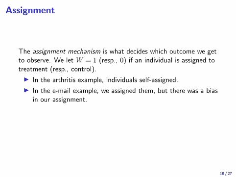
The assignment mechanism is what decides which outcome we getto observe. We let W = 1 (resp., 0) if an individual is assigned totreatment (resp., control).

I In the arthritis example, individuals self-assigned.

I In the e-mail example, we assigned them, but there was a biasin our assignment.

I Randomized assignment chooses assignment to treatment orcontrol at random.

10 / 27

Example 1: Potential outcomes

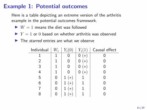
Here is a table depicting an extreme version of the arthritisexample in the potential outcomes framework.

I W = 1 means the diet was followed

I Y = 1 or 0 based on whether arthritis was observed

I The starred entries are what we observe

Individual Wi Yi(0) Yi(1) Causal effect

1 1 0 0 (∗) 02 1 0 0 (∗) 03 1 0 0 (∗) 04 1 0 0 (∗) 05 0 1 (∗) 1 06 0 1 (∗) 1 07 0 1 (∗) 1 08 0 1 (∗) 1 0

11 / 27

Example 2: Potential outcomes

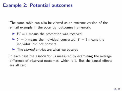
The same table can also be viewed as an extreme version of thee-mail example in the potential outcomes framework.

I W = 1 means the promotion was received

I Y = 0 means the individual converted; Y = 1 means theindividual did not convert.

I The starred entries are what we observe

In each case the association is measured by examining the averagedifference of observed outcomes, which is 1. But the causal effectsare all zero.

12 / 27

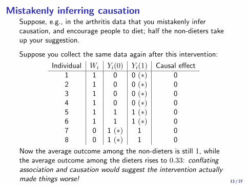
Mistakenly inferring causationSuppose, e.g., in the arthritis data that you mistakenly infercausation, and encourage people to diet; half the non-dieters takeup your suggestion.

Suppose you collect the same data again after this intervention:


1 1 0 0 (∗) 02 1 0 0 (∗) 03 1 0 0 (∗) 04 1 0 0 (∗) 05 1 1 1 (∗) 06 1 1 1 (∗) 07 0 1 (∗) 1 08 0 1 (∗) 1 0

Now the average outcome among the non-dieters is still 1, whilethe average outcome among the dieters rises to 0.33: conflatingassociation and causation would suggest the intervention actuallymade things worse!

13 / 27

Mistakenly inferring causationSuppose, e.g., in the arthritis data that you mistakenly infercausation, and encourage people to diet; half the non-dieters takeup your suggestion.

Suppose you collect the same data again after this intervention:


1 1 0 0 (∗) 02 1 0 0 (∗) 03 1 0 0 (∗) 04 1 0 0 (∗) 05 1 1 1 (∗) 06 1 1 1 (∗) 07 0 1 (∗) 1 08 0 1 (∗) 1 0

Now the average outcome among the non-dieters is still 1, whilethe average outcome among the dieters rises to 0.33: conflatingassociation and causation would suggest the intervention actuallymade things worse! 13 / 27

Estimation of causal effects

14 / 27

“Solving” the fundamental problem

We can’t observe both potential outcomes for each individual.

So we have to get around it in some way. Some examples:

I Observe the same individual at different points in time

I Observe two individuals who are nearly identical to each other,and give one treatment and the other control

Both are obviously of limited applicability. What else could we do?

15 / 27

The average treatment effect

One possibility is to estimate the average treatment effect (ATE)in the population:

ATE = E[Y (1)]− E[Y (0)].

In doing so we lose individual information, but now we have areasonable chance of getting an estimate of both terms in theexpectation.

16 / 27

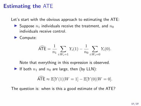
Estimating the ATE

Let’s start with the obvious approach to estimating the ATE:

I Suppose n1 individuals receive the treatment, and n0individuals receive control.

I Compute:

ATE =1

n1

∑i:Wi=1

Yi(1)−1

n0

∑i:Wi=0

Yi(0).

Note that everything in this expression is observed.

I If both n1 and n0 are large, then (by LLN):

ATE ≈ E[Y (1)|W = 1]− E[Y (0)|W = 0].

The question is: when is this a good estimate of the ATE?

17 / 27

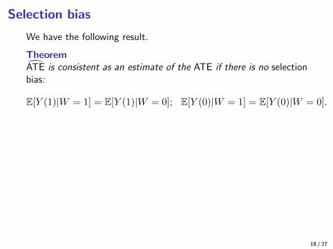
Selection bias

We have the following result.

TheoremATE is consistent as an estimate of the ATE if there is no selectionbias:

E[Y (1)|W = 1] = E[Y (1)|W = 0]; E[Y (0)|W = 1] = E[Y (0)|W = 0].

I In words: assignment to treatment should be uncorrelatedwith the outcome.

I This requirement is automatically satisfied if W is assignedrandomly, since then W and the outcomes are independent.This is the case in a randomized experiment.

I It is not satisfied in the two examples we discussed.

18 / 27

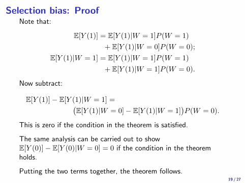
Selection bias: ProofNote that:

E[Y (1)] = E[Y (1)|W = 1]P (W = 1)

+ E[Y (1)|W = 0]P (W = 0);

E[Y (1)|W = 1] = E[Y (1)|W = 1]P (W = 1)

+ E[Y (1)|W = 1]P (W = 0).

Now subtract:

E[Y (1)]− E[Y (1)|W = 1] =(E[Y (1)|W = 0]− E[Y (1)|W = 1]

)P (W = 0).

This is zero if the condition in the theorem is satisfied.

The same analysis can be carried out to showE[Y (0)]− E[Y (0)|W = 0] = 0 if the condition in the theoremholds.

Putting the two terms together, the theorem follows.19 / 27

The implication

Selection bias is rampant in conflating association and causation.

Remember to think carefully about selection bias in any causalclaims that you read!

This is the reason why randomized experiments are the “goldstandard” of causal inference: they remove any possible selectionbias.

20 / 27

Randomized experiments

21 / 27

Randomization

In what we study now, we will focus on causal inference when thedata is generated by a randomized experiment.1

In a randomized experiment, the assignment mechanism is random,and in particular independent of the potential outcomes.

How do we analyze the data from such an experiment?

1Other names: randomized controlled trial; A/B test22 / 27

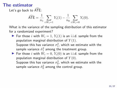
The estimatorLet’s go back to ATE:

ATE =1

n1

∑i:Wi=1

Yi(1)−1

n0

∑i:Wi=0

Yi(0).

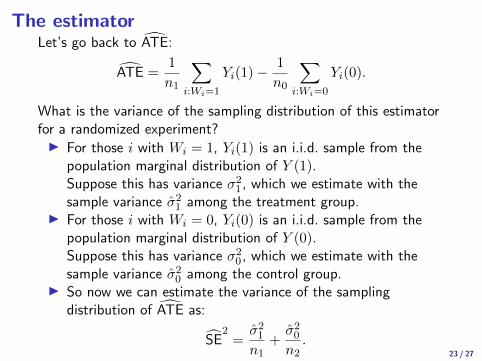
What is the variance of the sampling distribution of this estimatorfor a randomized experiment?

I For those i with Wi = 1, Yi(1) is an i.i.d. sample from thepopulation marginal distribution of Y (1).Suppose this has variance σ21, which we estimate with thesample variance σ21 among the treatment group.

I For those i with Wi = 0, Yi(0) is an i.i.d. sample from thepopulation marginal distribution of Y (0).Suppose this has variance σ20, which we estimate with thesample variance σ20 among the control group.

I So now we can estimate the variance of the samplingdistribution of ATE as:

SE2=σ21n1

+σ20n2.

23 / 27

The estimatorLet’s go back to ATE:

ATE =1

n1

∑i:Wi=1

Yi(1)−1

n0

∑i:Wi=0

Yi(0).

What is the variance of the sampling distribution of this estimatorfor a randomized experiment?I For those i with Wi = 1, Yi(1) is an i.i.d. sample from the

population marginal distribution of Y (1).Suppose this has variance σ21, which we estimate with thesample variance σ21 among the treatment group.

I For those i with Wi = 0, Yi(0) is an i.i.d. sample from thepopulation marginal distribution of Y (0).Suppose this has variance σ20, which we estimate with thesample variance σ20 among the control group.

I So now we can estimate the variance of the samplingdistribution of ATE as:

SE2=σ21n1

+σ20n2.

23 / 27

Asymptotic normality

For large n1, n0, the central limit theorem tells us that thesampling distribution fo ATE is approximately normal:

I with mean ATE (because it is consistent when the experimentis randomized)

I with standard error SE from the previous slide.

We can use these facts to analyze the experiment using the toolswe’ve developed.

24 / 27

CIs, hypothesis testing, p-values

Using asymptotic normality, we can:

I Build a 95% confidence interval for ATE, as:

[ATE− 1.96SE, ATE + 1.96SE].

I Test the null hypothesis that ATE = 0, by checking if zero isin the confidence interval or not (this is the Wald test).

I Compute a p-value for the resulting test, as the probability ofobserving an estimate as extreme as ATE if the nullhypothesis were true.

25 / 27

An alternative: Regression analysis

Another approach to analyzing an experiment is to use linearregression.

In particular, suppose we use OLS to fit the following model:

Yi ≈ β0 + β1Wi.

In a randomized experiment, Wi = 0 or Wi = 1.

Therefore:

I β0 is the average outcome in the control group.

I β0 + β1 is the average outcome in the treatment group.

I So β1 = ATE!

We will have more to say about this approach next lecture.

26 / 27

An example in R

I constructed an “experiment” where n1 = n0 = 100, and:

Yi = 10 + 0.5×Wi + εi,

where εi ∼ N (0, 1). (Question: what is the true ATE?)

lm(formula = Y ~ 1 + W, data = df)

coef.est coef.se

(Intercept) 9.9647 0.0953

W1 0.4213 0.1348

---

n = 200, k = 2

residual sd = 0.9532, R-Squared = 0.05

The estimated standard error on β1 = ATE is the same as theestimated standard error we computed earlier.

27 / 27

MS&E 226: Fundamentals of Data Science · MS&E 226: Fundamentals of Data Science Lecture 14:...

Documents

Transcript of MS&E 226: Fundamentals of Data Science · MS&E 226: Fundamentals of Data Science Lecture 14:...