MSc Thesis Process Algebraic - Performance...
78
TU Delft & Continental Engineering Services Master Thesis 1 MSc Thesis Process Algebraic - Performance Modeling of Embedded Software Ravindra Seetharama Aithal Abstract A compiler for embedded platforms has many optimization flags providing code size and speed improvement. Traditional profiling methods take lot of time to identify the best combination of the compiler flags to suit the requirement, especially if the software stack is very huge. AUTOSAR is one such growing software market in which there is a need for rapid performance assessment. In this thesis a means to estimate the performance of a program using the process algebraic language (PEPA) is investigated. The assembly program from trace is converted in to the PEPA model and the performance measures obtained by solving the model is verified against the actual execution time of the program. The experimental results provide valuable insights on the methodology. Master Thesis Number : CE-MS-2013-11 Faculty of Electrical Engineering, Mathematics and Computer Science, TU Delft
Transcript of MSc Thesis Process Algebraic - Performance...

TU Delft & Continental Engineering Services Master Thesis
1
MSc Thesis
Process Algebraic - Performance Modeling of Embedded Software
Ravindra Seetharama Aithal
Abstract
A compiler for embedded platforms has many optimization flags providing code size and
speed improvement. Traditional profiling methods take lot of time to identify the best
combination of the compiler flags to suit the requirement, especially if the software stack is
very huge. AUTOSAR is one such growing software market in which there is a need for rapid
performance assessment. In this thesis a means to estimate the performance of a program
using the process algebraic language (PEPA) is investigated. The assembly program from
trace is converted in to the PEPA model and the performance measures obtained by solving
the model is verified against the actual execution time of the program. The experimental
results provide valuable insights on the methodology.
Master Thesis Number : CE-MS-2013-11
Faculty of Electrical Engineering, Mathematics and Computer Science, TU Delft

TU Delft & Continental Engineering Services Master Thesis
2
MSc Thesis
Process Algebraic - Performance Modeling of Embedded Software
Submitted in partial fulfillment of the requirements for the degree of
MASTER OF SCIENCE
in
EMBEDDED SYSTEMS
by
Ravindra Seetharama Aithal
born in Bengaluru, India
Continental Engineering Services GmBH
AUTOSAR Center
Regensburg, Germany
Computer Engineering Department of Electrical Engineering Faculty of Electrical Engineering, Mathematics and Computer Science Delft University of Technology

TU Delft & Continental Engineering Services Master Thesis
3
MSc Thesis
Process Algebraic - Performance Modeling of Embedded Software
Laboratory : Computer Engineering
Master Thesis Number : CE-MS-2013-11
Committee Members :
Advisor : Arjan van Genderen , CE , TU Delft
Chairperson : Stephan Wong , CE , TU Delft
Member : Anne Remke , DACS , TU Twente
Member : Herbert Hofmann , CES-AC, Regensburg

TU Delft & Continental Engineering Services Master Thesis
4
Contents:
1. Introduction ……………………………………………………………………………. 5
2. Instruction Pipeline ………………………………………………………………….. 15
3. Cache ………………………………………………………………………………………..17
4. Probability Theory & Stochastic Processes…………………………………21
5. Performance Modeling………………………………………………………………30
6. PEPA…………………………………………………………………………………………..33
7. Design………………………………………………………………………………………...41
8. Experiments……………………………………………………………………………….66
9. Results……………………………………………………………………………………….67
10. Conclusion & Future Work………………………………………………………. 75
11. References………………………………………………………………………………..76
12. Appendix………………………………………………………………………………….78

TU Delft & Continental Engineering Services Master Thesis
5
1. Introduction:
1.1 Motivation
The state-of-art automotive vehicle (Passenger Car / Commercial Vechicle ) houses many
embedded systems like Enginer Management System (EMS) , Exhaust Gas Treatment ,
Adaptive Cruise Control (ACC) , Advanced Driver Assistance System (ADAS) etc offering
safety and comfort features. The basic embedded system unit of a vehicle is the Electronics
Control Unit (ECU). A typical car houses about 80-100 ECUs and about 30% cost of the
vehicle is attributed to the ECU. A ECU basically is a application specific hardware and
software co-design. The complexity of the automotive software is increasing year by year ,
with contribution of the number of patents for the software techniques being highest
combined with rapid innovation in the vehicle safety and comfort features.
The volume of the in-vehicle software is expected to increase by 30-40% in the coming years
[23]. Automotive applications correspond to about 17% of the embedded market . From
2012 to 2013 the automotive applications have increased by 2%[23].According to the survey
about 44% of the applications are started from scratch in 2013, and remaing 56% are the
upgrades or improvement on the earlier project. One of the main catalyst to the the rapid
changes in the automotive embedded market is AUTOSAR[1].
With increasing complexity of electronics in modern vehicle systems, the AUTOSAR
(AUTmotive Open System Architecture) community was born. The goal was to reduce this
complexity by means of standardized software modules and a layered architecture. The side-
effect of the standardization was that modules have to be developed in a generic way and
cannot be optimized for each single project as it was the case in the past. Although the
modules are highly configurable, the footprint and CPU load of AUTOSAR ECUs are strongly
increasing.
In AUTOSAR, the software modules are rapidly developed/reused/configured and delivered.
The entire automotive industry is migrating to the AUTOSAR. The software development
model doesn’t include a process of optimizing the software modules or any ad-hoc research
in between. Although numerous guidelines (MISRA [2] )are available to the developer, they
only address compliance to safety. Guidelines for optimization are not the same among
different hardware platforms. Hence the need of the hour is to develop a tool or
methodologies in which the developer can rapidly asses the performance of the software
modules validate the software reviews based on statistical measures. This project attempts
to provide the prototype of such a tool.

TU Delft & Continental Engineering Services Master Thesis
6
Continental Engineering Services GmBH – AUTOSAR Center is one of the members of the
AUTOSAR consortium. The R&D team of the company extensively reserches on the compiler
optimization flags and coding guidelines for the best performance result .The team also
specializes in developing, configuring the AUTOSAR modules , tailored to the needs of the
Original Equipment Manufacturers (OEM’S like BMW, VOLVO, etc) and delivering for the
series production.
1.2 Overview
Vowing to the rapid prototyping and validation of the software modules in AUTOSAR, and
the large time consumed by the traditional profiling methods, the need is to investigate the
possibility of assessing the performance measure with the help of modeling techniques.
Hence the problem statement is “development of a methodology for rapid code profiling
using process algebraic modeling language”.
In this project we statically evaluate embedded system software for different optimization
strategies/coding styles to meet the best performance without actually running on the
platform; Essentially a Static Code Analysis [3] .The source code is first fed through the
compiler with a particular optimization set or with a certain coding style. The compiler does
a transformation on the code and the assembly/trace file is generated. This intrinsically
provides information on how fast the hardware is going to run the code. A model (explained
in the subsequent sections) can be generated from the assembly code using the PEPA [4]
terminology.
PEPA stands for Performance Evaluation Process Algebra, is a tool supporting performance
modeling techniques. It’s simply an algebraic language which can be used to build a model of
the system and ascertain its performance matrix. We chose PEPA because it is a high-level
model specification language for low-level stochastic models, which allows the model of the
system to be developed as a number of interacting components undertaking certain
activities. A PEPA model has a finite set of components that correspond to indefinable parts
or roles of the system. PEPA allows us to model different actors of a system (for example in a
processor , instruction fetch unit, decode unit, execution unit, cache fetching etc.) and
analyze the effect of each of these different actors in unison or independently.
The hardware properties basically refer to the basic properties like single fetch or
superscalar processor, type and amount of cycles consumed by each instructions. Once we
obtain the performance ratings, the source code and the compiler can be tuned for the best
optimization results. In this case the performance can be obtained in the view of optimal
speed. For validating the model we can later run the actual code on the platform and
compare the results and as a feedback fine tune the model or the code.

TU Delft & Continental Engineering Services Master Thesis
7
Figure 1: Overview
A program can be visualized as a set of basic blocks with each consuming different time for
execution. The rate of execution of the basic blocks depends on
1) Distribution of the type of instructions in the blocks: In the sense the amount
of cycles that each of the instructions in the block consumes.
2) Memory segment in which the block is available: In the sense the availability
of the block in the main memory ( cache miss ) or in cache ( cache hit).
3) The property of the hardware in which the program is run: In the sense the
type of pipeline structure used (single fetch pipeline or dual fetch pipeline)
and also the amount of cycles consumed by each memory or cache access.
Correspondingly, based on these three classification, we can define three type of execution
rates.
1) Instruction Execution Rate : It’s the rate (1/time) at which the block of instruction
is executed by the processor.
2) Access Rate : It’s the rate at which the block is accessed either from memory or
from Cache
3) Effective rate: It’s the combined rate of execution of the instruction block.
The figure 2 shows the basic representation of the program in terms of blocks of instructions
, where r1,r2,r3…rN are the Instruction execution rate , AR1,AR2,AR3,…ARN are the Access
rates and ER1,ER2,ER3…ERN are the Effective rate before transformation. Similarly
r’1,r’2,r’3…r’N are the Instruction execution rate , AR’1,AR’2,AR’3,…AR’N are the Access rates
and ER’1,ER’2,ER’3…ER’N are the Effective rate after transformation.

TU Delft & Continental Engineering Services Master Thesis
8
Figure 2: Program representation in terms or basic blocks
Block access rate can be the memory access (MA) or cache access (CA). In order to identify
the change in rates of the basic blocks, CTMC (Continues Time Markov Chain) terminologies
are used with the help of the modeling language PEPA. The above representation of the
system can in turn be represented like a CTMC as shown in the following figure (with a
possible memory / cache access scenario).
Figure 3: CTMC representation of basic blocks
Each block is represented as a state in the CTMC with, exit rates being the rate at which the
block is executed and at the end of execution the state changes to the next block. The entry
rate to a state depends on the rate of accesses (CA/MA) and the exit rate from the preceding
state. From a CTMC, number of mathematical measure can be derived like the transient /

TU Delft & Continental Engineering Services Master Thesis
9
steady state probability matrices, Average response time, Cumulative distribution function
etc. which in turn gives the performance of the system. A compiler flag or combination of
compiler flags may alter the execution rate of the basic block of a program by
1) changing the type of instructions used ,
or
2) by shifting the memory in which the instruction is stored(in case of a Instruction
Cache)
and such changes can be easily identified in the performance measure of the CTMC. In order
to evaluate the performance measures we need to convert the assembly program in to a
process algebraic language model which can evaluate the performance measures. The
number of instructions in a basic block and rate of cache and memory access is directly
dependent on the issue fetching capability of the hardware platform. In the following
chapters we will discuss important performance measures, methodology and tools used for
performance estimation and the obtained results.
1.3 Challenges
The optimization criteria are the Speed of execution and the Memory consumption. Since
memory consumption estimation is already available in the current project setup we will
only consider estimating the speed of execution. A tool which can develop the PEPA script
from the assembly / trace file needs to be developed which would make methodology
scalable and less time consuming. Initial work can be dedicated to manual scripting and then
can be extended to automated scripting. If it becomes necessary to analyze the Boolean
predicate code then we also need to develop a script for the conversion to PEPA model.
If we use only assembly file for the analysis then it’s tedious to trace back the original source
in C and if we used Boolean predicate code [9] although it becomes easy to trace the source
in C, we miss the compiler optimization effects which can only be seen in the assembly file.
The best use-case is expected to be obtained during the experimentation. We start modeling
for a simple CPU like (single core, single pipeline, and single thread [10]) and in the near
future scale it to higher level systems.
1.4 Outcomes & Expectations
This method in a way produces the performance model [11] of the source code and the
compiler or the developers. They can estimate the effect of different coding styles, and
compiler optimizations (individually or in unison) statically & rapidly. The user can run the
tool interactively and can include CSL (Continuous Stochastic Logic) formula [12] checks to
evaluate satisfiability of stochastic criteria or estimate a stochastic measure.
This kind of static performance estimation is of high importance as they are less costly and
less time consuming. The entire setup will be rapid because of the fast solvers available in
the PEPA supported compilers and plug-in and easily scalable if we can develop tool for

TU Delft & Continental Engineering Services Master Thesis
10
conversion to the PEPA model from the respective sources. As an extension of the thesis, we
can test the project on some dedicated platforms to evaluate it further.
1.5 Background
a) AUTOSAR
AUTOSAR (AUTomotive Open System ARchitecture) is a worldwide development partnership
of car manufacturers, suppliers and other companies from the electronics, semiconductor
and software industry.
Paves the way for innovative electronic systems that further improve performance,
safety and environmental friendliness
Is a strong global partnership that creates one common standard: "Cooperate on
standards, compete on implementation"
Is a key enabling technology to manage the growing electrics/electronics complexity.
It aims to be prepared for the upcoming technologies and to improve cost-efficiency
without making any compromise with respect to quality
Facilitates the exchange and update of software and hardware over the service life of
the vehicle
AUTOSAR provides a common platform in which OEM’s , suppliers , tool providers etc can
collaborate with benefit that complexity of integration is reduced while improving the
flexibility , quality and reliability. The OEM’S benefit by enhanced design flexibility , reuse of
software modules across variants,simplified integration and reduced development costs. The
suppliers benefit from reduction of version proliferation and the ease of function
development. The tool developers can produce seamless and optimized landscapes for
tools.Thus AUTOSAR allows for smoother portability between different platforms. The car
production of AUTOSAR OEM members covers ~81% of the total cars produced worldwide.A
rapid growth of AUTOSAR’s market penetration between 2012 to 2016 is predicted such that
least 25% of the total number of ECUs produced in 2016 will have AUTOSAR inside[1]

TU Delft & Continental Engineering Services Master Thesis
11
Figure 4: From 4th AUTOSAR open conference[1]
b) Code analysis & Profiling
There are basically two types of analyisis that can be performed on a code.
1) Static analyisis. : is a technique of analyzing the source code statically without
actually running the program on the hardware.These techniques extract the
information about the oppertunity for the optimization in the source code by
analysis. Such technique are usually faster than the dynamic analysis but they are less
precise.
2) Dynamic analysis : is a technique of analyzing the source code by running it on a real
or virtual processor and profiling it. Profiling the program consists of collecting the
oppertunities during the execution of the program in order to guide effective
optimization.The optimizations can be performed either on the source code,
assembly code or by re-compilation guided by the collected information.There are
two types of dynamic analysis
a. By Instrumentation : In this technique several instructions are inserted in
source level or assembly level or in the binary level. Instrumentation adds
code to increment counters at the entry or exit function which will simulate
the harware performance counters or even simulate hardware to get
synthetic event counts. The instrumentation technique may dramatically
increase the execution time such that the time measurement become
redundant. It also becomes time inefficient in case of a huge software stack
making profiling itself time consuming. Example MAQAO[31].
b. By Sampling : In this method measurement points are inserted during short
time intervals.The validity of the result depends on the choice of the
measurement.Example Prof and Gprof.

TU Delft & Continental Engineering Services Master Thesis
12
c) Process algebra
Process algebra is a method for formally modeling concurrent systems. Process algebra
provides a tool for the high-level description of interactions, communications, and
synchronizations between a collection of independent agents or processes. They also
provide algebraic laws that allow process descriptions to be manipulated and analyzed,
and permit formal reasoning about equivalences between processes. Examples of
process calculi include CSP, CCS, ACP, LOTOS ,π-calculus, the ambient calculus, PEPA, the
fusion calculus and the join-calculus [37].
d) Model checking
Given a model of a system, Model checking refers to exhaustively and automatically
checking whether the model meets a given specification.In general Model checking delas
with verifying the correctness of a finite state systems.In order to achieve this , the
model of the system and the specifications are fomulated in terms of precise
mathematical language.
1.6 Related Work
Emphirical/Process algebraic model based performance prediction system for compiler
optimization evaluation is an exclusive area of reaseach and it’s the topic for the literature
survey.
Qualitative analysis tools using model checking are available. Model checking and static
analysis are automated techniques promising to ensure that the correctness of the software
and to find certain class of bugs automatically. One of the drawbacks of the model checker is
that they typically operate on a low level semantic abstraction making them suitable for
small software stack, but less so for larger stack and when the soundness is paramount as in
the case of industrial C/C++ code containing pointer arithmetic , unions templates and alike.
Goanna is built on an automata based static analysis framework as described in [25].The tool
maps the C/C++ program to its Control Flow Graph (CFG) and labels the CFG with
occurrences of syntactic constructs of interests automatically. The CFG together with the
labels can be seen as a transition system with atomic propositions, which can be easily
mapped to the input of a model checker (NuSMV) or translated in to a Kripke structure. The
basic checks which can be performed by Goanna are access violations, memory leaks array
and string overruns, division by zero, unspecified, non-portable, and/or dangerous
constructs and security vulnerabilities. Model checking has also been used to check the
malicious code patterns by [26]

TU Delft & Continental Engineering Services Master Thesis
13
One of the quantitative measures of a program execution is its Worst Case Execution Time
WCET. METAMOC [27] (Modular Execution Time Analysis using Model Checking) is a
modular method based on model checking and static analysis , that determines the safe and
tight WCET for programs running on platforms featuring caching and pipelining. The method
works by constructing the UPPAAL [28] model of the program being analyzed and annotating
the model with information from the interprocedural value analysis. The program model is
then combined with a model of the hardware platform and the model checked for the
WCET. The tool is retargetable for platforms ARM7,ARM9 and ATMEL AVR 8-bit. The pipeline
and cache behavior are modeled in UPPAAL. In [29] it is debated that model checking is not
suitable for WCET analysis but in [30] its shown that model checking can actually improve
the WCET estimates for hardware with caching. In the master thesis [38] modeling the
Analytical Software Design blocks as queueing systems is investigated in order to reduce the
implementation errors in the integration phase of the software project.
Qualitative performance measure of a code produced by the compiler is essential to get high
performance. Previously the quantitative measure was assesed by the number of
instructions. With recent generation of micro processors the matrices are no longer
valid.The number of branches , use of specific instructions , Caches which have been
introduced to improve the temporal locality and other architectural feature like instruction
prefecting are responsible for the performance. Modular Assembler Quality Analyzer and
Optimizer (MAQAO) [31] is a tool performing the static analyis on the assembly code. The
tool takes assembly as input, constructs the CFG , call flow graph, loop structure . Furthur
analysis can be scripted using the SQL scripting symantics. Some of the analysis that can be
performed by MAQAO are gathering statistics like number of NOPs,number of bundles with
three way branching or number of loops, generating the histogram of basic blocks size in a
function or histogram of the IPC (instruction per count) , code pattern such as defecient
sequence,missing prefetches detection , detection of the optimization performed by the
compiler etc.
The lack of statically available information may prevent user to apply different compiler
optimization or program transformation aggressively or applying them together.
Performance aware compilation systems address this problem by a combination of run-time
testing and static information. Dynamic compilation systems such as [32] enable the code
generation at the runtime allowing the compiler to exploit the knowledge about the input
values and hence generate more efficient code. In another case [33] at run-time the best
combination of the optimizations is chosen by evaluating the performance of each of the
versions. In case of performance prediction systems, empherical model of the code is used
as static estimators to guide the application of the program transformations with goal to
select the highest possible performance as done in [34]. In several other cases the
performance of the application is modeled based on analytical expressions as done in [35].

TU Delft & Continental Engineering Services Master Thesis
14
Performance oriented modeling techniques [36] offer an alternative way of enabling the
compiler to derive and select a set of program transformations . This modeling approach is
valuable in scenarios in which the application takes extremely long time to execute making
profiling impractical or even predict the performance on future architectures. Using the
target architecture description in terms of the number of functional units , pipelines and
their depth the compiler can derive a set of performance analytical expression for a set of
scenarios and determine for each of these scenarios what the expected performance is in
terms of consumed clock cycles and peak performance and execution of the code section
would take. For example if one of the various memory references in the basic block casues a
TLB miss that leads to pipeline stall (due to data dependencies) this leads to a substantial
decrease in overall performance.For different scenario emperical model can be obtained or
by target architecture cycle level accurate simulations.

TU Delft & Continental Engineering Services Master Thesis
15
2. Instruction Pipeline
2.1 Pipelines:
A assembly program is a contiguous set of instructions derived from the original C program.
Each instruction in an assembly program takes certain cycles for execution. An instruction
pipeline is a technique used in the design of computers architecture to increase their
instruction throughput (the number of instructions that can be executed in a unit of time).
Pipelining does not reduce the time to complete an instruction, but increases the number of
instructions that can be processed at once.
Each instruction is split into a sequence of dependent steps. The first step is always to fetch
the instruction from memory; the final step is usually writing the results of the instruction to
processor registers or to memory. Pipelining seeks to let the processor work on as many
instructions as there are dependent steps, rather than waiting until the current instruction is
executed before admitting the next one. Pipelining lets the computer's cycle time be the
time of the slowest step, and ideally lets one instruction complete in every cycle.
A pipeline typically includes the following 5 steps
1. Instruction fetch (IF)
2. Instruction decode and register fetch (ID)
3. Execute (EX)
4. Memory access (MEM)
5. Register write back (WB)
The following diagram shows the typical 5-stage instruction pipeline and the way the
instruction is processed in each stage.

TU Delft & Continental Engineering Services Master Thesis
16
Figure 5 : Single Fetch Instruction Pipeline
2.2 Superscalar CPU
A superscalar CPU incorporates instruction level parallelism within a single processor and
hence achieving faster throughput than a single fetch processor. A superscalar processor
executes more than one instruction during clock cycle by simultaneously dispatching
multiple instructions
The following diagram shows the typical dual fetch 5-stage instruction pipeline.
Figure 6 : Dual Fetch Instruction Pipeline
Similar to the single fetch CPU even in a dual fetch CPU, the instructions are fetched
sequentially . The CPU checks dynamically the data dependencies between instructions at
the run time

TU Delft & Continental Engineering Services Master Thesis
17
3. Cache
A cache is a small amount of memory which operates more quickly than main memory. Data
is moved from the main memory to the cache, so that it can be accessed faster. The cache
memory performance is the most significant factor in achieving high processor performance.
Cache works by storing a small subset of the external memory contents, typically out of its
original order. Data and instructions that are being used frequently, such as a data array or a
small instruction loop, are stored in the cache and can be read quickly without having to
access the main memory. Cache runs at the same speed as the rest of the processor, which is
typically much faster than the external RAM operates at. This means that if data is in the
cache, accessing it is faster than accessing memory.
When the processor needs to read from or write to a location in main memory, it first checks
whether a copy of that data is in the cache. If so, the processor immediately reads from or
writes to the cache, which is much faster than reading from or writing to main memory. A hit
in a cache is when the processor finds data in the cache that it is looking for. A miss is when
the processor looks for data in the cache, but the data is not available. In the event of a miss,
the cache controller unit must gather the data from the main memory, which can cost more
time for the processor. Most modern CPUs have at least three independent caches: an
instruction cache to speed up executable instruction fetch, a data cache to speed up data
fetch and store, and a translation look aside buffer (TLB) used to speed up virtual-to-physical
address translation for both executable instructions and data. The data cache is usually
organized as a hierarchy of more cache levels
3.1 Cache Entry
Data is transferred between memory and cache in blocks of fixed size, called cache lines.
When a cache line is copied from memory into the cache, a cache entry is created. The cache
entry will include the copied data as well as the requested memory location which is called
as a tag.
When the processor needs to read or write a location in main memory, it first checks for a
corresponding entry in the cache. The cache checks for the contents of the requested
memory location in any cache lines that might contain that address. If the processor finds
that the memory location is in the cache, a cache hit has occurred (otherwise, a cache
misses).

TU Delft & Continental Engineering Services Master Thesis
18
In the case of
a cache hit, the processor immediately reads or writes the data in the cache line.
a cache miss, the cache allocates a new entry, and copies in data from main memory.
Then, the request is fulfilled from the contents of the cache
Cache row entries usually have the following structure:
The data block (cache line) contains the actual data fetched from the main memory. The tag
contains a part of the address of the actual data fetched from the main memory. Flag bits
indicate whether a cache block has been loaded with a valid data(valid bit).A instruction
cache has only one flag bit(valid bit) per cache row where as a data cache has two flag bits
(valid bit and dirty bit) per cache row.
The size of the cache is the amount of main memory data it can hold. This size can be
calculated as the number of bytes stored in each data block times the number of blocks
stored in the cache. (The number of tag and flag bits is irrelevant to this calculation, although
it does affect the physical area of a cache).
An effective memory address is split (MSB to LSB) into the tag, the index and the block
offset.
The index describes which cache row (which cache line) that the data has been put in. The
index length is log2(cache rows) bits. The block offset specifies the desired data within the
stored data block within the cache row. Typically the effective address is in bytes, so the
block offset length is log2(byte per data block) bits. The tag contains the most significant bits
of the address, which are checked against the current row (the row has been retrieved by
index) to see if it is the one we need or another, irrelevant memory location that happened
to have the same index bits as the one we want. The tag length in bits is (address_length –
index_length – block_offset_length).

TU Delft & Continental Engineering Services Master Thesis
19
3.2 Cache Replacement Policy
In order to make room for the new entry on a cache miss, the cache may have to evict one of
the existing entries. The heuristic that it uses to choose the entry to evict is called the
replacement policy. The fundamental problem with any replacement policy is that it must
predict which existing cache entry is least likely to be used in the future. Predicting the
future is difficult, so there is no perfect way to choose among the variety of replacement
policies available. The following replacement policies exist.
Least Recently Used (LRU)
Round Robin (or FIFO)
Most Recently Used (MRU)
Random Replacement
3.3 Cache Associativity
The replacement policy decides where in the cache a copy of a particular entry of main
memory will go. If the replacement policy is free to choose any entry in the cache to hold the
copy, the cache is called fully associative. Accordingly there are 2-way,4-way associative
cache. If each entry in main memory can go in just one place in the cache, the cache is called
to be directly mapped.
3.4 Cache Performance:
A processor with a cache first looks in the cache for data (or instructions). On a miss, the
processor then fetches the data (or instructions) from main memory. On a miss, this process
takes longer time than an equivalent processor without a cache.
There are three ways a cache gives better net performance than a processor without a
cache:
A hit (read from the cache) is faster than the time it takes a processor without a
cache to fetch from main memory. The trick is to design the cache so we get hits
often enough that their increase in performance more than makes up for the loss in
performance on the occasional miss. (This requires a cache that is faster than main
memory).
Multiprocessor computers with a shared main memory often have a bottleneck
accessing main memory. When a local cache succeeds in satisfying memory
operations without going all the way to main memory, main memory bandwidth is
freed up for the other processors, and the local processor doesn't need to wait for
the other processors to finish their memory operations.
Many systems are designed so the processor often read multiple items from cache
simultaneously -- either 3 separate caches for instruction, data, and TLB; or a multi

TU Delft & Continental Engineering Services Master Thesis
20
ported cache; or both -- which takes less time than reading the same items from
main memory one at a time.
A processor without a cache has a constant memory reference time, = + E
A processor with a cache has an average memory access time, = m * + + E
where
m is the miss ratio
is the time to make a main memory reference
is the time to make a cache reference on a hit
E accounts for various secondary factors (memory refresh time, multiprocessor
contention, etc.)
Cache hit/miss is evident in any assembly program and both the programmer and the
compiler are the reason for the cache miss in a program. Depending on the cache
configuration, the cache hit miss scenario can be modeled from the assembly program and
the overall delay can be evaluated statically the best configuration can be selected.

TU Delft & Continental Engineering Services Master Thesis
21
4. Probability Theory & Stochastic Processes
4.1 Probability
If n is the number of possible outcomes of an system, each of them equally likely, nA is the
number of events in favor of event A , the Pr[A] = nA / A. Set of all possible outcomes is called
the sample space S. The following axioms hold good.
Pr [S] =1
Given A ∩ B = φ , events A & B are mutually exclusive then Pr [A U B] = Pr[A] + Pr[B]
& Pr [A U B] = Pr[A] + Pr[B] - Pr [A ∩ B]
If two events A and B are independent Pr [A ∩ B] = Pr [A] Pr [B] .
Conditional probability Pr [A | B] = Pr [A ∩ B] / Pr [B]
Law of total probability Pr [A ] = ∑
, Bk ∩ Bj = φ
4.2 Random Variables
A variable whose possible values are the numerical outcome of a random phenomenon is
called as a random variable. More formally a random variable is a measurable function from
a probability space (s,Ṩ,P) into a measurable space (s’, Ṩ’) known as the state space. Also a
random variable X is a real function whose domain is the probability space s and such that:
1. The set {X ≤ x} is an event for any real number x.
2. The probability of the events { X = +∞} and {X = -∞ } equals zero.
There are two types of random variables,
Discrete time random variable takes values in discrete steps denoted as X[k] where k=
0,1,2,3… ∞ .
Continuous time random variable takes in continuous steps denoted as X(t) where 0≤t<∞
4.2.1 Cumulative Distribution Function
A cumulative distribution function describes the probability that a real valued random
variable X with a given probability distribution will be found at a value less than or equal to x
F(x) = Pr(X≤x)

TU Delft & Continental Engineering Services Master Thesis
22
4.2.2 Probability Density Function
A probability density function describes the relative likelihood for the random variable to
take a given value.
f(x) =
(Fx)
4.3 Probability Distribution Functions
1) Exponential Distribution
A random variable X is said to be exponentially distributed if it satisfies the probability
density function f(x) = α e-αx α,x ≥ 0 where α is the rate at which the event occurs .
The cumulative distribution function is F(x) = 1 - α e-αx
The mean , or average of the distribution ,μ = 1/α . Variance Var[X] = 1/α2.
Exponential distribution satisfies memoryless property , Pr[X≥t +T | X > t] = Pr[X > T ]
2) Poisson Distribution
A random variable X is said to be Poisson distributed if its satisfies the probability density
function ,
f(x,k) = λk e-λ / k!.
The cumulative distribution function F(x,k) = e-λ ∑
μ = Var[X] = λ
4.4 Discrete Time Markov Chain
A stochastic process formally denoted as { X(t) , t ∈ T} is a sequence of random variables X(t)
, where the parameter t – time runs over an index set T. The state space of the stochastic
process is the set of all possible values of the random variables X(t) and each of these
possible values is called the state of the process. If the index set T is a countable set , X [k] is
a discrete stochastic process. If T is continuous X(t) is a continuous stochastic process.
A stochastic process { X(t) , t ∈ T} is a Markov process if the future state of the process only
depends on the current state of the process and not on its past history. Formally, a
stochastic process { X(t) , t ∈ T} is a continuous time Markov process if for all t0 < t1 < t2 <
……tn+1 of the index set T and for any set {x0,x1,x2,….xn+1} of the state space it holds that

TU Delft & Continental Engineering Services Master Thesis
23
Pr[X(tn+1)= |X(t0)= ,….,X(tn)= ]=Pr[X(tn+1)= |X(tn)= ]
The Markov property states that at any times s > t > 0, the conditional probability
distribution of the process at time s given the whole history of the process up to and
including time t, depends only on the state of the process at time t. In effect, the state of the
process at time s is conditionally independent of the history of the process before time t,
given the state of the process at time t.
A discrete time Markov chain { X [k], k ∈ T} is a stochastic process whose state space is
finite or countably infinite set with index set T = {0, 1, 2….} obeying
Pr[ = | = ,…., = ]=Pr[ = | = ]
A Markov process is called a Markov chain if its state space is discrete. The conditional
probabilities Pr [ = j| = i] are called the transition probabilities of the Markov chain.
In general, these transition probabilities can depend on the (discrete) time k. A Markov chain
is entirely defined by the transition probabilities and the initial distribution of the Markov
chain Pr [ = ] .
By using the definition of the conditional probability it can be shown that the complete
information of the Markov chain is obtained if, apart from the initial distribution, all time
depending transition probabilities are known as per the formula.
Pr[ = ,…., = ] = ∏
If the transition probabilities are independent of time k i.e if = Pr [ = j| = i] the
Markov chain is called stationary. In a state space S with N states (where N = dim(S) can be
infinite) Since Xk can take N possible values, we denote the corresponding state vector at
discrete-time k by s[k] = [s1[k] s2[k] · · · sN [k]] with s(i)[k] = Pr[Xi = k].Hence, s[k] is a 1 × N
vector. Since the state Xk at discrete-time k must be in one of the N possible states and
hence ,
∑
or,
in vector notation, s[k].u = ∑ where uT = [1 1 · · · · · · · 1].
In a stationary Markov chain the states Xk+1 and Xk are connected by the equation of total
probability Pr[Xk+1 = j] = ∑
for all j or in vector notation s[k+1] = s[k].
P where P is the transition probability matrix and it must hold that ∑
, means
that at discrete-time k, there certainly occurs a transition in the Markov chain, possibly to
the same state as at time k-1. A matrix P satisfying this relation is called stochastic matrix. If
Pij is independent of k then its called time homogeneous Markov chain.
Given an initial state vector s[0], the general solution of s[k] = s[0] .Pk and s[k+n] = s[0].Pk+n

TU Delft & Continental Engineering Services Master Thesis
24
The elements of matrix Pn are called n-step transition probabilities,
= Pr[ = j | =i]
The transition probability matrix P is of the form
Figure 7 : Transition probability matrix
Since it must hold for any initial state vector s[0], by choosing s[0] = [0 …..0 1 0…….0] (all
column zero except for ith column ) which expresses that Markov chain starts from one of
the possible states , say state i , then s[1] = [Pi1 Pi2 Pi3 ………PiN]
4.4.1 The hitting time and Sojourn time
If A is a subset of states , A ⊂ S , the hitting time TA is the first positive time the Markov
chain is in a state of set A , thus for k ≥ 0 , TA = min(k : ∈ A ). The sojourn time of state i
in a Markov chain is the amount of time the system spends in state i before leaving to state
j≠i.
4.4.2 Transient ,Recurrent and Absorbing states
The probability that a Markov chain , starting at state i will come to state j is given as
= Pr[ < ∞| X0 = j] .
If i = j then , is the probability of returning to state in i. If Pii =1 then the state is a
recurrent and if < 1 , then the state is transient. If = 1 and = 0 for i≠j then it’s called
an absorbing state.
4.4.3 The steady state vector
The state of the system with k→∞ is called the steady state and the vector = lim k→∞ s[k]
is called the steady state vector and it must hold that or for each component
= ∑

TU Delft & Continental Engineering Services Master Thesis
25
for 1≤j≤N = such that ∑
The solution of is obtained from the following equation
4.5 Continuous Time Markov Chain
For the continuous-time Markov chain {X(t),t≥ 0} with N states, the Markov property can be
written as
Pr[X(t + τ)=j|X(τ)=i, X(u)=x(u), 0≤u< τ) ] = Pr[X(t + τ)= j|X(τ)= i ]
and reflects the fact that the future state at time t+ τ only depends on the current state at
time τ . Similarly as for the discrete-time Markov chain, we assume that the transition
probabilities for the continuous-time Markov chain {X(t),t≥ 0} are stationary, i.e.
independent of a point τ in time,
Pij(t) = Pr[X(t + τ) = j|X(τ) = i] = Pr[X(t) = j|X(0) = i]
Similar to discrete time Markov chain, the state vector s(t) in continuous time components
sk(t) = Pr[Xk = k ] , with P(t) being the transition probability matrix ,satisfies
s(t+ τ) = s(τ) P(t) & P(t+ u) = P(t) . P(u)= P(u).P(t)
Since Markov chain should be in one of the N states
∑
, with P(0) = .
Given the infinitesimal generator Q = P’(0) =
the transition probability matrix
is differentiable for all t≥0 and hence ,
P’(t) = P(t) Q = Q P(t)

TU Delft & Continental Engineering Services Master Thesis
26
It can be proved that ∑
where =
≥ 0 and ≤ 0 ,
which implies that sum of rows of Q is zero . of Q are the derivatives of the probabilities
and they reflect the change in the probability from state i towards state j and are called
rates.
4.5.1 Properties of
If = - ≥ 0 then, ∑
. This demonstrates that Q is bounded if and only
if the rates are bounded. For finite state Markov processes, are finite (since qij are
finite), but, if = ∞, the state is called instantaneous since when the process enters this
state, it immediately leaves the state. Continuous-time Markov chains with all states non-
instantaneous are called conservative.
4.5.2 Properties of Q
Q has the property that P(t) = eQt = (
)
and can be explicitly given as follows
Figure 8: Infinitesimal generator matrix
4.5.3 Steady state
If the finite state Markov chain is irreducible, the steady state exists. Since steady state
vector doesn’t change over time
P’(t) =0 implies that Q(Pl) = (Pl)Q = 0 , where Pl=
P(t). Similar to the argument with discrete time markov chain , the steady state (row) vector
is solution of Q = 0. Since
sk(t) = and
s’k(t) = 0.
Alternatively = s(0) (Pl) =
(0) eQt
The main difference between discrete and continuous-time Markov chains lies, apart from
the concept of time, in the determination of the number of transitions. In case of a
continuous time Markov chain, the sojourn time in a discrete chain is deterministic and all

TU Delft & Continental Engineering Services Master Thesis
27
times are equal to 1. The sojourn times τj of a continuous-time Markov process in a state j
are independent, exponential random variables with mean 1/
4.6 Embedded Markov chain :
A method of finding π of an ergodic continuous-time Markov chain, Q, is by first finding its
embedded Markov chain (EMC). EMC is a regular discrete-time Markov chain, also called as a
jump process. Each element of the one-step transition probability matrix of the EMC, S, is
denoted by sij, and represents the conditional probability of transitioning from state i into
state j.The relation between the steady state vector of the continuous time Markov chain
and its corresponding embedded discrete time markov chain v are,
= / ∑
and = ( ) / ∑
The classification in the discrete-time case into transient and recurrent can be transferred
via the embedded Markov chain to continuous Markov processes.
4.7 Uniformization:
Uniformization is a method to compute the transient solution of a finite state CTMC. The
method involves construction of analogous DTMC , where transition occur to an exponential
distribution with the same parameter in every state and hence the name uniformization.
For a continuous time Markov chain with infinitesimal generator matrix Q , the uniformized
transition matrix P( ) is given as follows
{
∑
Where q is a rate value which is chosen to be greater than the magnitude of all the rates
within the generator matrix , i.e q ≥ . In matrix notiation it can be written as
,
P =
, where I is the Identity matrix
For a starting distribution , the distribution at time t, with system having completed n
hops can be derived as

TU Delft & Continental Engineering Services Master Thesis
28
∑
This representation shows, that “a continuous time Markov Chain can be described by a
discrete Markov Chain with transition matrix P as defined above where jumps occur
according to a Poisson process with intensity qt”
4.8 First Passage Time Analysis
Consider a finite, irreducible , CTMC with n states {1,2,3…..n} and the infinitesimal generator
matrix Q. If X(t) denotes the state of the CTMC at time t (t≥0) , then the first passage time
from a source state i into a non-empty set of target states is given as
T (t) = inf{u > 0 : X(t+u) ∈
| X(0) = i } ∀ t≥0
For stationary time-homogeneous CTMC T is independent of t, so T
(t) = inf{u > 0 : X(u)
∈ | X(0) = i } . T
is associated with probability density function, f(x) of the random
variable by the relation
Pr(a< T <b) = ∫
(0≤ a < b)
The cumulative density function (CDF) of passage is obtained by multiplying the probability
of being in a target state j after exactly n hops within time t by the probability of performing
n within the time t,
∑
The probability density function (PDF) of a passage is the probability of performing n hops at
exactly time t to reach state j is given as
Hence the Passage time equations for CDF and PDF are as follows,
∑ ( (∑
))
∑ ( (∑
))

TU Delft & Continental Engineering Services Master Thesis
29
4.9 Poisson process
A continuous time stochastic process {X(t) , t≤0} satisfying the following properties is called a
poisson process
(i) X(0) = 0
(ii) ∀ t0 = 0 < t1 < t2….<tn , the increments X(t1) – X(t0) , X(t2) – X(t1) , ….,X( tn) – X(tn-1)
are independent random variables
(iii) For t≥ 0, s > 0 and non negative integers k, the increments have Poisson
distribution
Then Pr[ X(t+s) – X(s) = k ] = (λt)k e- λt/ k! ,
λ is the rate of the Poisson process with mean of the process = λt
The above process is a homogenous Poisson process where the number of events in an
interval (t, t+τ) follows a poisson distribution.
4.9.1 Properties
1) A Poisson process {X(t) , t ≥0} with rate λ > 0 and denoted by t0 = 0 <t1<t2…. the
successive occurrence times of events, then the interarrival times τn = tn – (tn -1) are
independent identically distributed exponential random variables with mean 1/λ . In other
words, the cumulative distribution function , F(x) = Pr[τn ≤ x] = 1 – e-λx
2) If X(t) and Y(t) are two independent poisson processes with rates λx and λy , then
Z(t) = X(t) + Y(t) is also a poisson process with rate λx + λy
3) A Poisson process is the most basic form of a CTMC, i.e a chain of independent
identically distributed states with mean sojurn time of 1/qj

TU Delft & Continental Engineering Services Master Thesis
30
5. Performance modeling
Performance modeling is a process of modeling system performance considering various
sytem parameters with the objective of proactively predicting the performance statically. To
obtain the performance model of a system, its required to denote the system in abstract
form of which represents average behavior. In order to perform this several operational laws
are applied. The advantages of the laws are that,
1) They are very general and make no assumptions about the behavior of the random
variables characterizing the system.
2) They are very simple meaning that they can be applied quickly and easily by almost
anyone.
Based on a few simple observations of the system , by applying these simple laws, we can
derive more information. Using this information as input , we can gradually build up a more
complete picture of the behavior of the system.
Operational laws are built on observable variables. These are values which we could derive
from watching a system over a finite period of time. Consider a system receiving requests
from its environment. Each requests generates a job in the system . when the job has been
processed by the system the system responds to the environment with the completion of
the requests. Based on this analogy , we can identify the following variables
Figure 9 : A sample system model
T : the length of time we observe the system
A : the number of request arrivals we observe
C : the number of request completions we observe
B : the total amount of time during which the system is busy (B<T)
N : The average number of jobs in the system.

TU Delft & Continental Engineering Services Master Thesis
31
From these observed values we can derive the following four quantities:
λ = A/T, the arrival rate,
X = C/T, the throughput or completion rate,
U = B/T, the utilization,
S = B/C, the mean service time per completed job
Response time = Service time + Wait time , where response time is the time between the
initiation and completion of the response to a request and wait time is the time between the
submission of the request and initiation of the response. We assume that the system is job
flow balanced , meaning that number of arrivals is equal to number of completions during
an observation period and hence A = C => λ = X.
5.1 Little’s Law
It states that the average number of jobs in a system is equal to the product of the
throughput of the system and the average time spent in that system by a job
If average number of jobs in the system is N , and W is the average residence time of the
jobs in the system , then the throughput of the system X = N / W
5.2 Forced flow law
It states that the throughput at the ith resource is equal to the product of the throughput of
the system and the visit count at that resource.
If is the visit count of the ith resource , the ratio of number of completions at that
resource to the number of system completions is = /C. Hence if is the throughput of
the system at ith resource then = X.
5.3 Utilization Law
It states that the utilization of a resource is equal to the product of the throughput of that
resource and the average service requirement at that resource.
The total amount of the service Si that a system job generates at the ith resource is called
the service demand . = . The utilization of a resource is the percentage of time that
the ith resource is in use processing the job
= = X .

TU Delft & Continental Engineering Services Master Thesis
32
5.4 Residence Time Law
It states that the average residence time or average response time of a job in the system will
be the sum of the product of its average residence time at each resource and the number of
visits it makes to that resource.
W = ∑
5.5 Queueing theory
Queueing theory describes basic phenomena such as the waiting time, the throughput, the
losses, the number of queueing items, etc. in queueing systems. A queueing system basically
consists of a) Arrival process b) Queueing process c) Service process and d) Departure
Process
Figure 10 : Queueing model
The general syntax is A/B/n/K/m, where A specifies the interarrival process, B the service
process, n the number of servers, K the number of positions in the queue and m restricts the
number of allowed arrivals in the queueing system. Examples for both the interarrival
distribution A and the service distribution B are M (memoryless or Markovian) for the
exponential distribution, G for a general distribution and D for a deterministic distribution.
The traffic intensity of a Queueing system , also called Load or Utilization ρ = E[x]/ E[τ] = λ/μ
, where λ is the mean interarrival rate and μ is the mean service rate. Applying Little’s law ,
the average number of jobs in the system E[Ns] equals to the average arrival rate λ times the
average time spend in the system E[T], E[Ns] = λ . E[T].
5.6 Queueing Models
The M/M/1 queue (with unlimited positions in the queue , which will not be indicated in the
notation) consists of a Poisson arrival process of jobs with exponentially distributed
interarrival times, a service process with exponentially distributed service time, one server
and an infinitely long queue. Similarly M/M/1/K queue consists of a Poisson arrival process
of jobs with exponentially distributed interarrival times , a service process with exponentially
distributed service time, one server and with a queue capacity of K.The following tables
summarizes different performance measures of M/M/1 and M/M/1/K queue

TU Delft & Continental Engineering Services Master Thesis
33
Performance Measures M/M/1 M/M/1/K
Traffic intensity, ρ λ/ μ λ/ μ
Utilization , U (per server) Ρ ρ(1 – ((1- ρ). ρK/(1- ρK+1))
Average number of jobs in the system , E[Ns]
ρ/(1- ρ) ρ/(1- ρ) – ((K+1). ρ(K+1))/ (1- ρK+1))
Average response time, E[T] 1/ μ (1- ρ) N/ λ*1/(1- ((1- ρ). ρK /(1- ρK+1))
Table 1 : Queueing model parameters
6. PEPA
PEPA is a stochastic process algebra designed for modeling computer and communication
systems introduced by Jane Hillston. The language extends classical process algebras such as
Milner's CCS and Hoare's CSP by introducing probabilistic branching and timing of
transitions.
PEPA consists of set of agents which engage in action . Models can be constructed from
components which engaged in activities. The structured operational (interleaving ) semantics
of language is used to generate a labeled transition system (LTS) . The behavior of the model
is dictated by the semantic rules (Structure Operational Semantics) governing the
combinator of the language. The possible evolutions of a model are captured by applying the
rules exhaustively generating a labeled transition system. The resulting system can be
viewed as a graph in which each node can be viewed as a state of the model and the arcs
representing the actions which can cause the model to move from one state to another i.e a
CTMC .
Figure 11 : PEPA overview
Rates are drawn from the exponential distribution and PEPA models are finite-state and so
give rise to a stochastic process (CTMC). Thus the language can be used to study quantitative
properties of models of computer and communication systems such as throughput,
utilization and response time as well as qualitative properties such as freedom from
deadlock. The language is formally defined using a structured operational semantics in the
style invented by Gordon Plotkin.

TU Delft & Continental Engineering Services Master Thesis
34
PEPA has four combinators, prefix, choice, co-operation and hiding. Prefix is the basic
building block of a sequential component: the process (a, r).P performs activity a at a rate r
before evolving to behave as component P. Choice sets up a competition between two
possible alternatives: in the process (a, r).P + (b, s).Q either a wins the race (and the process
subsequently behaves as P) or b wins the race (and the process subsequently behaves as Q).
The co-operation operator requires the two "co-operands" to join for those activities which
are specified in the co-operation set: in the process P < a, b> Q the processes P and Q must
co-operate on activities a and b, but any other activities may be performed independently.
Finally, the process P/{a} hides the activity a from view (and prevents other processes from
joining with it).
6.1 Syntax & Properties
Given a set of action names, the set of CCS processes is defined by the following BNF
grammar:
P ::= (a, λ).P | P + Q | P <L> Q| P/L | A
The parts of the syntax are, in the order given above
(i) action :
The process (a, λ).P can perform an action a at a rate λ and continue as the process P.
(ii) choice :
The process P+Q may behave as either the process P or the process Q.
(iii) Cooperation :
The processes P and Q exist simultaneously and behave independently for actions whose
names do not appear in <>. For actions whose names appear in <>, the action must be
carried out jointly and a race condition determines the time this takes. E.g. P< a,b >Q : P
and Q are synchronized over a and b
(iv) Parallel :
The processes P and Q exist simultaneously and behave independently. E.g. P < > Q.
(v) Hiding:
The process P behaves as usual for action names not in L, and performs a action for action
names that appear in < L >. E.g. P/{a}.
(vi) Process identifier:
write to use the identifier A to refer to the process P.
TU Delft & Continental Engineering Services Master Thesis
35
6.1.1 Synchronization
PEPA has a bounded capacity for synchronization . When two activates with different rates
are synchronized by co-operation operator, the rate of the shared activity is reduced to the
minimum of the apparent rates of the activity in the co-operating components.
6.1.2 Activity Rate
When an activity α is enabled by a process P = (α, λ ) , the completion of the activity is
delayed for a period determined by the associated exponential distribution. The probability
that the activity α happens within a period of time t , is given by the cumulative distribution
function F(t) = 1 - .If several activities are enabled at the same time each will have their
own associated timer.When the time t expires the activity is said to be completed w.r.t an
external observer. A activity is preempted or aborted if another activity completes first.
The apparent rate of a component P with respect to the action type α , is the total capacity
of the component P to carry out activities of type α , denoted by rα(P)
6.1.3 Time Homogeneity
PEPA models are time-homogeneous , since all the activities are time-homogeneous, i.e the
rate and type of activates enabled by a component are independent of time.
6.1.4 Irreducibility & Positive recurrence
Only the PEPA models with finite number of states are solved, i.e the models should be
irreducible and positive recurrent (strongly connected) which are expressed in terms of the
derivation graph. This means that in the system whenever we chose a path it must
eventually return to the point where the original choice is made possibly with different
outcome
6.1.5 Exponential Property
The memory less property of the exponential distribution makes the recording of the
residual time of an activity redundant.
6.1.6 Structured Operation Semantics
PEPA is defined using Plotkin-style structured operational semantics. The rules are described
as follows
Prefix (α ,r ). E → E

TU Delft & Continental Engineering Services Master Thesis
36
Choice
→
→
,
→
→
Cooperation
→
→
, α not belongs to L
→
→
→
, αϵL ,
where R = r1/rα(E) . r1/rα(F) min( rα(E) , rα(F) ) .
Hiding
→
→
, α not belongs to L
→
→
, αϵL
Constant
→
→
6.1.7 Multiway co-operation
Co-operation in PEPA can be multiway. Two , three , four or more partners may cooperate
and they all need to synchronize for the activity to happen.
6.1.8 Solving PEPA
The generated CTMC are solved using the linear algebra in terms of the equilibrium
behavior. IPC and PEPA eclipse plugin solve the equations and derives the performance
measures.
6.1.9 State space Explosion problem
The solver in PEPA relies on constructing the N*N infinitesimal generation matrix Q and N
dimensional probability vector π , where N is the size of the state space. Sometimes the size
exceeds what could be handled by the memory and its called states space explosion
problem.
It can be avoided by three methods
State space reduction by Aggregation
Stochastic simulation over discrete state space
Fluid approximation of the state space

TU Delft & Continental Engineering Services Master Thesis
37
We use Aggregation method , in which the states space is partitioned in to number of
smaller states, and replace each set by a macro state. By using the Markov property “The
sojourn times τj of a continuous-time Markov process in a state j are independent,
exponential random variables with mean 1/qj” , we can view the macro state as a state in a
new CTMC.
6.2 PEPA Plug-in project:
The PEPA Plug-in Project [14] is a software tool for the Markovian analysis of PEPA models.
The tool is implemented as a collection of plug-ins for Eclipse.The PEPA Plug-in contributes
an editor for the language and views which assist the user during the entire cycle of model
development. Static analysis is used for checking the well-formedness of a model and
detecting potential errors prior to inferring the derivation graph of the system. A well-
formed model can be derived, i.e. the underlying Markov process is extracted and the
corresponding state space can thus be navigated and iterated via the State Space view.
Finally, the CTMC view allows numerical steady-state analyses such as activity throughput
and component utilization.
The plug-in will report errors in the model function:
deadlock,
absorbing states,
static synchronization mismatch (co-operations which do not involve active
participants).
The plug-in also generates the transition graph of the model , computes the number of
states, formulates the Markov process matrix Q , communicates the matrix to a solver. The
plug-in provides a simple pattern language for selecting states from the stationary
distribution
The plug-in integrates the Hydra [15] compiler which can be used to process the well formed
PEPA model for performance measures like
Transient Analysis & Steady State analysis : Measures the transient and steady state
probabilities of the system
Passage Time Analysis : Measures the probability of the system response time to be
at a certain value.
Throughput, Utilization & Population: Measures the percentage occupation and
utilization of the action components of the system.

TU Delft & Continental Engineering Services Master Thesis
38
6.3 IPC
Ipc stands for Imperial PEPA Compiler. It’s a compiler for solving PEPA models and for performing various measurements. In ipc there are five general kinds of measurements that can be specified.
Steady-state
Passage-time
Average response time
Transient
Count measures Special probe components are used to specify complex performance measurements and use the simpler interface of specifying activities of interest. The first four kinds of measurements require ’start’ and ’stop’ actions to be given by the user, while a count measure requires only one set of action names. A passage-time measurement is used to measure between two events. The user specifies a set of start actions, the observation of the model performing any one of these actions will start the measurement. The user also specifies a set of stop actions and the measurement is terminated when the model performs any actions within that set. This can be done with the following command line:
ipc --source <source actions> --target <target actions> <PEPA file name>
In addition to this, the start , stop and time step can also be specified in the command line as follows
ipc --source <source actions> --target <target actions> --start-time <start time> --stop-time <stop time> --time-step <time step> <PEPA file name>
The average response time measurement is also used to measure between two events, with
a start and end action or a set of start and end actions with the following command
ipc --source <source action> --target <target action> --average-response <PEPA file name>
The following command can be issued to generate the state space view of the model
ipc --dot-file <PEPA file name >

TU Delft & Continental Engineering Services Master Thesis
39
The ipc compiler is integrated in to the tool for analysis of the 1-PIPELINE , 2-PIPELINE &
Cache PEPA models. We use both Passage time measurement and Average response time
measurement for the analysis.
6.4 PEPA Example
The following PEPA script models 2 processes, P and Q synchronizing over actions b and c
r = 1.0; s = 2.0; t = 1.5; // Rate of transitions P1 = (a, r).P2; // Transition P1 - > P2 P2 = (b ,r).P3 + (c ,s).P4; // System can do a Transition P2 -> P3 or P2 ->P4 (it has a choice) P3 = (d ,r).P4; // Transition P3 -> P4 P4 = (e ,r).P1; // Transition P4 -> P1 Q1 = (b, t).Q2; // Transition Q1 -> Q2 Q2 = (c, t).Q1; // Transition Q2 -> Q1 P1<b,c>Q1 // P1 & Q1 paths synchronize over actions b & c , i.e b & c should be //performed at the same time in both P1 & Q1 Figure 14 : Example PEPA script
In the first stage the model is parsed and checked for errors. The tool generated CTMC is as
shown below.
Figure 14 : Abstract State space View
The system has 2 components P & Q , which will co-operate / synchronize over actions b & c
. By synchronization it means that P & Q will adjust each other to carry out actions b & c in
unison where as in other cases they can carry out their actions independently but no actions
can be missed.
The Passage time cumulative distribution with source action as a and target action as c is as
shown in the Figure 15. This measure indicates, (as described in the section 4.8 ) the
probability that the system starting from the state with action a , reaches state with action c
(the number of hops determined by the actions) within a specific time. The effect of change
in the rates r, s & t on the time to reach the target state with 99.99% probability is as shown
below.

TU Delft & Continental Engineering Services Master Thesis
40
Figure 12 : Passage time CDF
The average response time (ART) of the model with source action as a and target action as c
with different values of r,t and s along with time to reach 99.99% probability are as
tabulated below. From the table its certain that the model runs faster when the rates
arer=2,t=1 & s=1.
Table 2 : Rate vs ART
0
0.1
0.2
0.3
0.4
0.5
0.6
0.7
0.8
0.9
1
0 1 2 3 4 5 6 7 8 9 10 11 12 13 14 15
Pro
bab
ility
Time
CDF
r=1,t=1.5,s=1
r=2,t=1,s=1
r=2,t=1,s=1.5
r=1,t=1.5,s=2
Rate Average Response Time
Time to reach 99.99% probability
r = 1.0 , t =1.5, s= 1.0 2.5 9.8
r = 2.0 , t =1.0, s= 1.0 1.75 7.8
r = 2.0 , t =1.0, s= 1.5 1.75 7.8
r = 1.0 , t =1.5, s= 2.0 2.333 9.73

TU Delft & Continental Engineering Services Master Thesis
41
7. Design
In this chapter the different modeling approaches and the performance measures obtained in each is discussed.
7.1 Single fetch Pipeline Modeling
A typical 5 stage pipeline instruction execution sequence is as shown in the figure 5. For the
sake of PEPA modeling we consider each instruction is made to undergo three actions.
1) Fetch : if
2) Decode :id
3) Execution : exe
The execution action can involve Memory Read/Write and or register Read/Write actions
which is abstracted to a single exe action. The rate of execution (r) for each action is the
inverse of the cycle taken for completion. Hence rate of if = 1, rate of id = 1 and rate of exe =
(1/C). In an instruction set, each type of instruction has its own cycle of execution which is
directly used in the PEPA equations.
Each instruction execution is imagined to be a Process component P(i) , which will
synchronize with each subsequent instructions P(i+1) , P(i+2 )….etc. As we can see from the
figure 2, the if, id of instruction 2 must synchronize with id , exe (MEM,WB) of instruction
1. Similarly Instruction 3 must synchronize with the respective actions of instruction 1 & 2.
However we can see that till the id actions , the rate of the synchronized action matches ,
but with exe action, the rate will be different for different type of instructions. PEPA assumes
bounded capacity: that is, a component cannot be made to perform an activity faster by
cooperation, so the rate of a shared activity is the minimum of the apparent rates of the
activity in the cooperating components. So if we synchronize with exe can execute at the
rate of 1 or ½=0.5 or ⅓ =0.333 or ¼=0.25 etc , we tend to pull the combined exe,if,id rate to
the lowest of the set. (For example if we are synchronizing actions with rates 1,0.5,0.333
then the combined rate of execution is min{1,0.5,0.333}=0.333). This will be wrong
interpretation of the system. However for the sake of experiments we will also model the
system by synchronizing the exe. It should also be noted that while synchronizing the actions
we should maintain common name for the actions to be synchronized. The following
approaches are possible for modeling.
The number of instructions for modeling is limited to 4 because
beyond 4 processes, the PEPA undergoes a population explosion in some approaches.
In order to maintain uniformity in experimentation

TU Delft & Continental Engineering Services Master Thesis
42
Consider the following set of 4 instructions to be executed in a 5 stage pipeline
mr r5, r6
stmw r7,r8
mr r4, r8
bl r7
Approach 1:
The model of the system in approach 1 is as shown in the figure 19. In this approach we
synchronize only the if and id stages of the instructions.
Figure 13 : Approach 1 overview

TU Delft & Continental Engineering Services Master Thesis
43
Figure 14 : Approach 1 state space
Approach 2:
The model of the system in approach 21 is as shown in the figure. In this approach we
synchronize the if, id and exe of the instructions.
Figure 15 : Approach 2 overview

TU Delft & Continental Engineering Services Master Thesis
44
Figure 16: Approach 2 state space
The following table summarizes the Average response time measure for each approach. We
use if as the source action and the set of all the exe’s as the target action to evaluate ART.
Table 3 : Comparison
0
0.1
0.2
0.3
0.4
0.5
I0 I1 I2 I3
% P
op
ula
tio
n
Processes
Population
Approach 1
Approach 2
Type Average Response Time
Approach 1 2.94
Approach 2 3.40

TU Delft & Continental Engineering Services Master Thesis
45
Similar to the evaluation of ART use if as the source action and the set of all the exe’s as the
target action to evaluate Passage time CDF.
Figure 17 : Population, Throughput & Passage time CDF comparison
0.145
0.15
0.155
0.16
0.165
0.17
bl3 cm cm1 cm2 cm3 if mr0 mr2 stmw1
% T
hro
ugh
pu
t
Actions
Throughput
Approach 1
Approach 2
0
0.2
0.4
0.6
0.8
1
0 1 2 3 4 5 6 7 8 9 101112131415161718192021222324252627282930
Pro
bab
ility
Time
Passage time CDF
Approach 1
Approach 2

TU Delft & Continental Engineering Services Master Thesis
46
7.2 Dual fetch 1-Pipeline Modeling
A typical dual fetch-5 stage pipeline instruction execution sequence is as shown in the below
figure 26. For the sake of PEPA modeling we consider each instruction is made to undergo
three actions.
1) Fetch : if
2) Decode :id
3) Execution : exe
In case of a dual fetch pipeline, two instructions are fetched simultaneously and are executed in parallel. Each instruction in a first set , execution is imagined to be a Process component P(i) , which will synchronize with each subsequent instructions P(i+1) , P(i+2 )….etc. As we can see from the figure 2, the if of the two instructions fetched is common and should synchronize; id of instruction 2 must synchronize. Similarly Instruction 3 must synchronize with the respective actions of instruction 4. However we can see that till the id actions , the rate of the synchronized action matches. Also id action on both the instruction set can be synchronized. Depending on the actions used for synchronization there are 2 approaches. Approach 1
In this approach the if of the first two instructions will synchronize with each other, followed by id of the first 2 instructions along with the if of the 2nd instruction set, followed by the id of the 2nd instructions set.
Figure 18 : Approach 1 overview

TU Delft & Continental Engineering Services Master Thesis
47
Figure 19: Approach 1 state space
Approach 2
In this approach the if of the first two instructions will synchronize, followed by id of the first 2 instructions along with the if of the 2nd instruction set, followed by the exe of the 1st set with the id of the 2nd instructions set , followed by the exe of the 2nd set.
Figure 20 : Approach 2 overview

TU Delft & Continental Engineering Services Master Thesis
48
Figure 21: Approach 2 state space
Approach 3
In this approach the if of the first two instructions will synchronize, followed by id of the first 2 instructions. Along with the similar actions of the 2nd instruction set.
Figure 22 : Approach 3 overview
Figure 23 : Approach 3 state space

TU Delft & Continental Engineering Services Master Thesis
49
Figure 24: Population, throughput & passage time CDF comparison
0
0.2
0.4
0.6
0.8
I0 I1 I2 I3
% P
op
ula
tio
n
Processes
Population
Approach 1
Approach 2
Approach 3
0
0.1
0.2
0.3
0.4
0.5
bl3 cm cm2 if mr0 mr2 stmw1 cm1
% T
hro
ugh
pu
t
Actions
Throughput
Approach 1
Approach 2
Approach 3
0.00E+00
2.00E-01
4.00E-01
6.00E-01
8.00E-01
1.00E+00
0 5 10 15 20
Pro
bab
ility
Time
Passage Time CDF
Approach 1
Approach 2
Approach 3

TU Delft & Continental Engineering Services Master Thesis
50
The average response time of models in three different approaches is as shown in the
following table. We use if as the source action and the set of all the exe’s as the target action
to evaluate ART.
Type Average Response Time
Approach 1 3.28
Approach 2 3.18
Approach 3 2.47
Table 4 : Comparison
In order to choose the best approach, we compare the traditional performance measure i.e
Cycle per instruction (CPI) with ART of the corresponding PEPA model. The cycle per
instruction is given by the formula
CPI = ∑
Where ICi : Number of Instructions of type i
Ci : Number of cycles consumed by instruction of type i
IC : Total instruction count
In the below table I0,I1,I2,I3 in sequence are the number of execution cycles (EXE) of the instructions. For 4 instructions the value of CPI for a single fetch 5 stage pipeline can be calculated using the formula , CPI = ( Total Cycles taken for I0 + I1 + I2 + I3 ) / 4 Total cycle taken by an Instruction = cycle for IF+ cycle for ID + Cycle for EXE . In case of a dual fetch CPU the CPI is 0.5 times the CPI of a single fetch CPU.

TU Delft & Continental Engineering Services Master Thesis
51
Table 5 : CPI vs ART comparison

TU Delft & Continental Engineering Services Master Thesis
52
The following graph shows the variation of the CPI and ART with different combination of
the instruction cycles.
Figure 25 : CPI vs ART comparison
We take different combination of the instruction types with number of instructions being 4
and compare the variation of the CPI in case of the single fetch & dual fetch pipeline
execution model, against the corresponding average response time. Only for Approach 1 in
case of single fetch , and approach 3 in case of dual fetch pipeline, the CPI is in proportion to
the average response time as shown in the figure 25. Along with this reason, those two
models also avoid the bounded rate capacity drawback of the PEPA. Hence we choose
approach 1 of single fetch and approach 3 of dual fetch for final modeling. Since the plots of
CPI and ART are proportional, this could be the closest possible model of program execution
by the processor.
0 1 2 3 4 5 6 7 8 9 10 11 12 13 14 15 16 17 18 19 20 21 22 23 24 25 26 27 28 29 30 31 32 33 34 35 36 37
0
1
2
3
4
5
6
7
Instruction combination
CP
I & A
RT
Comparison of ART & CPI
Single Fetch CPI
Single Fetch ART
Dual Fetch CPI
Dual Fetch ART

TU Delft & Continental Engineering Services Master Thesis
53
7.3 Single fetch Cache Memory Access Modeling
A typical single fetch -5 stage pipeline instruction execution, along with cache and memory
action sequence is as shown in the figure 26. For the sake of PEPA modeling we consider
each instruction is made to undergo the following actions.
1) Cache access : ca
2) Memory Access :ma
3) Fetch : if
4) Decode :id
5) Execution : exe
In case of a single fetch pipeline, single instruction is fetched. The synchronization of actions as described in 1-pipeline modeling is followed. The algorithm for finding if the instruction is available in cache or in memory as shown in the figure 36 is used. If the instruction is available in the cache, then ca action appears in the equation else ma action appears in the equation. For showing the modeling example, we assume a scenario that 1st and 3rd instructions are available in cache and 2nd and 4th instructions are available in memory. We also assume to a show a distinctive rates of execution of the instruction blocks , that cache access takes 4 cycles and memory access takes 10 cycles.
Figure 26 : Overview

TU Delft & Continental Engineering Services Master Thesis
54
Average response time = 6.43
Figure 27: Population, throughput & passage time CDF
0
0.1
0.2
0.3
0.4
0.5
0.6
I0 I1 I2 I3
%p
op
ula
tio
n
Processes
Population
single fetch
0.00E+00
2.00E-02
4.00E-02
6.00E-02
8.00E-02
1.00E-01
1.20E-01
%th
rou
ghp
ut
Actions
Throughput
Throughput
0
0.2
0.4
0.6
0.8
1
0 20 40 60 80 100 120 140
Pro
bab
ility
Time
Passage Time CDF
single fetch

TU Delft & Continental Engineering Services Master Thesis
55
7.4 Dual fetch Cache Memory Access Modeling
A typical dual fetch -5 stage pipeline instruction execution, along with cache and memory
action sequence is as shown in the figure 28. For the sake of PEPA modeling we consider
each instruction is made to undergo three actions.
1) Cache access : ca
2) Memory Access :ma
3) Fetch : if
4) Decode :id
5) Execution : exe
In case of a dual fetch pipeline, two instructions are fetched simultaneously and are executed in parallel. The synchronization of actions as described in dual fetch 1-pipeline modeling is followed. The algorithm for finding if the instruction is available in cache or in memory as shown in the figure 36 is used. If the instruction is available in the cache, then ca action appears in the equation else ma action appears in the equation. For showing the modeling example, we assume a scenario that 1st and 2nd instructions are available in cache and 3rd and 4th instructions are available in memory. We also assume to a show a distinctive rates of execution of the instruction blocks, that cache access takes 4 cycles and memory access takes 10 cycles.
Figure 28 : Overview

TU Delft & Continental Engineering Services Master Thesis
56
Figure 29 : State space
0
0.2
0.4
0.6
I0 I1 I2 I3
%P
op
ula
tio
n
Processes
Population
dual fetch
0.00E+00
5.00E-02
1.00E-01
1.50E-01
2.00E-01
2.50E-01
bl3 ca cm cm2 if ma mr0 mr2 stmw1
% T
hro
ugh
pu
t
Actions
Throughput
dual fetch

TU Delft & Continental Engineering Services Master Thesis
57
Figure 30 : Population, Throughput & passage Time CDF
Average Response time = 6.90985
7.5 Observations from the models
From the state space of the models we can observe that ,starting from the initial
state we cannot miss any actions and hence the corresponding rate of finishing it
Synchronized action must be performed & hence can verify and validated model
from trace
Over synchronization reduces the state-space and gives lower average response time
In CTMC or in a exponential distribution the mean expectation time = E[Tx]=μ= 1/λ
where is the rate (parameter of an exponential distribution). Hence,
o Higher the cycle taken by the instruction block=> lower the rate => Higher
the response time of the model
o Lower the cycle taken by the instruction block => higher the rate => Lower the
response time of the model
For the passage time CDF the same analogy as for the average response time holds
good
0
0.1
0.2
0.3
0.4
0.5
0.6
0.7
0.8
0.9
1
0 20 40 60 80 100 120 140
Pro
bab
ility
Time
Passage Time CDF
Dual fetch

TU Delft & Continental Engineering Services Master Thesis
58
7.7 Assembly to Pipelined PEPA model conversion
Given a assembly program, we can visualize each block B(i) {i=1,2,3,….N} as a independent Poisson process with a mean rate defined by λi= (1/ARTi). Each such block itself is comprised of instruction fetch process, decode process and execute process ,executed at a mean rate λ. From the postulate of the CTMC which states that “The sojourn times τj of a continuous-time Markov process in a state j are independent, exponential random variables with mean 1/qj”. The converse implies that if the sojourn times of a random stochastic process are distributed with the mean rate of 1/qi then it must be CTMC and CTMC is a strong Poisson process. In a Poisson process time between each events is exponentially distributed. From PEPA modeling, we can observe that each activity is assigned a time that is exponentially distributed. From these we can obtain the following inferences.
1. Each block of the system can then be visualized as a part of Periodic CTMC , in which each state X(t) corresponds to the execution of the each block B(i).
2. Finding the stochastic measures of the CTMC gives us the performance measures of the program. Passage time analysis is one such stochastic measure used to find the time between the occurrences of two events in the stochastic process.
3. Passage time analysis evaluates how fast , starting from an initial state B0 the system
can jump to state Bn . i.e t at P(t)≥99.99% with source action as blk0 and target action as blkn. With change in the compiler flags used, we expect a change in the value of t.
Figure 31 : Assembly to CTMC conversion

TU Delft & Continental Engineering Services Master Thesis
59
Vowing to the limitation in the number of instructions being used for modeling because of the states space explosion problem in PEPA and also the delay in producing the Average response time (ART ) by the IPC and PEPA plugin , we can visualize a scenario as shown in the figure 33. We divide the assembly program in to blocks of 4 as fetched by the processor, convert them to PEPA model and calculate ART for each block. We then can visualize that the each block executes at a rate defined by (1/ART), (by the property of CTMC). With the rates of each block available we can then view each block as a macro- state component in the abstract block model. Solving the abstract block model provides the performance measure of the whole system.The last equation BlkN = (blkN,rN).Blk1 ; basically indicates that there is choice for the system to continue the execution from the beginning. The scripting is divided in to two parts
1) Assembly to PEPA instruction model construction and evaluation of ART 2) Conversion of PEPA instruction model to Abstract block model and evaluation
of final performance measure.
Figure 33: Performance Measurement

TU Delft & Continental Engineering Services Master Thesis
60
7.6 Hardware Details The SPC56ELxx microcontroller is based on the e200z4 Power Architecture and targets the
electric power steering, chassis, and safety applications that require a high safety integrity
level. The e200z4 processor family is a set of CPU cores that implement low-cost versions of
the Power Architecture technology. The e200z4 core is a dual-issue, 32-bit design with 64 -
bit general purpose registers (GPRs). The host processor core of the SPC56ELxx is a CPU from
the e200z4 family of compatible Power Architecture cores. The device’s 5-stage pipeline dual
issue core provides a high efficiency allowing high performance with minimum power
dissipation.
The processor integrates a pair of integer execution units, a branch control unit, instruction
fetch unit and load/store unit, and a multi-ported register file capable of sustaining six read
and three write operations per clock cycle. Most integer instructions execute in a single clock
cycle. Branch target perfecting is performed by the branch unit to allow single-cycle
branches in many cases.
Figure 33: Block Diagram of e200z4

TU Delft & Continental Engineering Services Master Thesis
61
The key features of e200z4 can be summarized as follows
Dual issue , 32-bit power ISA-compliant core
Implementation of the VLE for reduced code foot print
In-order execution and termination
Precise exception handling
Branch processor unit (BPU)
Dedicated branch address calculation adder
Branch target perfecting using and 8-entry branch target buffer (BTB)
Supports independent instruction and data access to different memory subsystems,
such as SRAM and flash memory by means of independent instruction and data bus
interface units
Load/store unit
64-bit general-purpose register file
4Kbyte , 2/4-way set-associative instruction cache
From the block diagram of the hardware it can be seen that , the instruction memory unit fetches 2/4 instructions from the memory or cache , and the instruction fetch unit fetches 2 instructions at a time executing in a pipelines structure as shown in the figure 7. The hardware can be configured to fetch 4 instructions at a time which suits our modeling approach.
7.7 Methematical Analysis Lets assume that we have 3 blocks of instructions executing at the rate r1,r2, & r3.According to the figure 46, the corresponding PEPA model would be Blk0 = (blk0,r1).Blk1; Blk1 = (blk1,r2).Blk2; Blk2 = (blk2,r3).Blk0; Blk0 The following table summarizes the ARTs & time to reach 99.99% probability with source action as blk0 and target action as blk2 for few variations of r1,r2,&r3
r1 r2 r3 ART Time to reach
99.99% probability
1 1 1 2 10
1 1 0.5 3 16
1 0.5 1 3 11.2
1 0.5 0.5 4 19.4
Table 6 : Rate comparison

TU Delft & Continental Engineering Services Master Thesis
62
Lower the block execution rate, higher is the cycles consumed by the block and hence higher the time consumed by the block. In such scenario, if we have a set of blocks with lower block execution rate, the cycle consumed by the block set is higher. But the corresponding ART & time to reach 99.99% probability is higher. Hence we need to consider the case with higher ART or higher time to reach 99.99% probability as the scenario with higher execution time of the program.
Mathematically ,we can analyze the situation as follows. From the equation of the passage time CDF we have
∑
In each of the cases we mention in the table q value varies depending on the rate distribution in the CTMC. For a fixed value of rate q , the t has to increase such that becomes close to 0 making F(q,t)~ 99.99%. In other words in case of higher execution time of the programs, q is lower such that t will increase to reach 99.99% probability.

TU Delft & Continental Engineering Services Master Thesis
63
Figure 34: instruction trace (PowerPC)
Figure 35 : Assembly instructions (PowerPC)

TU Delft & Continental Engineering Services Master Thesis
64
The flow chart for the identification of cache hit/miss and cache entry if the replacement
policy is FIFO is as follows.
No
Yes
Yes
No
Yes
No
Yes
Figure 36: FIFO Replacement Algorithm
Input Cachesize ,Block
Size, associativity, Trace
file
Filter trace file (remove
invalid strings, numbers etc)
Read Address & Instructions
No of blocks = Cache Size / Block Size No of sets = Cache Size ( Associativity * Block Size)
Initialize Cache_Array (No of Sets) ( Associativity) & FIFO_Array(No of Sets)
If not end
of file
Set = (Address / Block Size) % No of set Tag = (Address/(Block Size * No of set)
i = 0
i < associativity & Cache_Array(set)(i) =tag
Found = 1
If found ==1
Use ca action with
corresponding rate
Use ma action with
corresponding rate
Insert FIFO_Array(set) in
Cache_Array(Set)(tag)
Increment FIFO_Array(set)
If FIFO_Array(set) == Associativity
FIFO_Array(set)
=0
END
i + +

TU Delft & Continental Engineering Services Master Thesis
65
8. Experiments
In order to evaluate the tool we compiled some random programs provided under WCET
benchmark suit [37] . This benchmark suit provides programs having different combinations
of the 10 different software properties namely : I ,E,S,L,N,A,B,R,U,F where
I = uses include files. E = calls external library routines. S = always single path program (no potential flow dependency on external variables). L = contains loops. N = contains nested loops, A = uses arrays and/or matrixes. B = uses bit operations. R = contains recursion. U = contains unstructured code. F = uses floating point calculation.
Results obtained with the modeling the programs available in this suite give assurance that
the methodology is scalable and we can apply the techniques on any program.We use
instruction trace file generated by the WindRiver DIAB tool as the input to a script which
converts it to the corresponding PEPA model.From the tool we generate the ART and the
Passage Time CDF with time to reach 99.99% probability as the performance measures for
comparison. We use the dual fetch configurations described in the design chapter for
modeling.We apply different compilation flag combination initially and see the actual run
time on the hardware and the modeled results.. A summary of the compilation flags is given
in the appendix. We use iTrace/PRO profiler/debugger to measure the program execution times.
The instruction trace is generated by the wind-river DIAB compiler tool using the ELF file as the
input.
In another experiment we compiled some random programs with the loop-unroll
optimization compared against no-unroll , with linear search compared against binary search
We use all the 4 configurations described in the design chapter and under each configuration
we experiment with both optimized and un-optimized versions and compare the values

TU Delft & Continental Engineering Services Master Thesis
66
9. Results
9.1 Modeling Simple Programs
The following table shows the comparison of ARTs and the Peak passage time for each of the
different configuration for the different code optimization implementation for a program
which counts the number of bits in a given digit and binary and linear search algorithms.
Figure 52 : Loop unroll vs No unroll

TU Delft & Continental Engineering Services Master Thesis
67
Figure 53 : Linear Search vs Binary Search
9.1.1 Result Analysis
From the plot 51, it can be seen that the response of the program rises steeply (increase in
the slope , more faster to reach 100% probability) from no optimization to unroll
optimization in all the 8 configurations. The slope of the graph increase from single fetch to
dual fetch vindicating the fact that the throughput of the processor indeed increases from
single fetch to dual fetch. However the effect of cache & memory reduces the slope of the
graph as the access time to memory and cache are added to the model and the combined
execution time increases due to this effect. Nevertheless we can observe that the unroll
configuration has a better cache/memory access response compared to the cache memory
response of the un-optimized version. Also the cache memory response of the dual fetch
version is much better than the single fetch version.

TU Delft & Continental Engineering Services Master Thesis
68
9.2 Modeling Benchmark Programs
a) bs.c ( Property : L = contains loops & A = uses arrays and/or matrixes )
Figure 39: bs with different compiler combination
From the table it can be seen that the program doesn’t change much w.r.t different
combination of the compiler flags (means inherently optimized). The execution time ,ART
and t at P(t) =99.99% are flat lines
0
20
40
60
80
100
120
140
0 1 2 3 4 5 6 7 8 9 10 11 12 13 14 15
Tim
e
Compiler flag combination
bs
Execution time (ns)
ART
t at P(t)≥99.99%

TU Delft & Continental Engineering Services Master Thesis
69
b) countbit.c ( Property : L = contains loops , B = uses bit operations )
Figure 40: countbit with different compiler combination
It can be seen that the ART and t at P(t) ≥99.99% follow close proportional relation w.r.t the
execution time and we can easily identify that Xsize-opt + Xwhole-prog-opt=0x9 is the best
optimization.
0
20
40
60
80
100
120
140
160
180
200
0 1 2 3 4 5 6 7 8 9 10 11 12 13 14 15
Tim
e
Compiler flag combination
countbit
Execution time (ns)
ART
t at P(t)≥99.99%
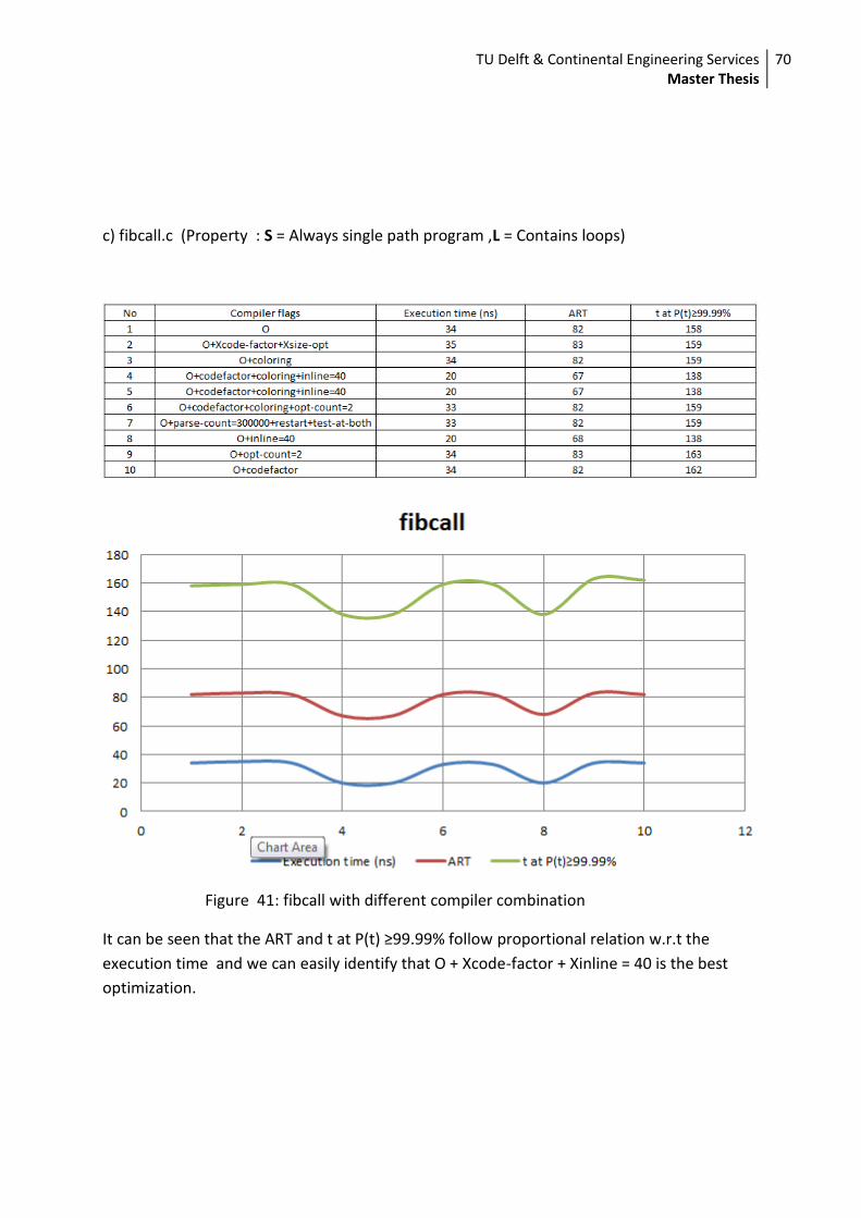
TU Delft & Continental Engineering Services Master Thesis
70
c) fibcall.c (Property : S = Always single path program ,L = Contains loops)
Figure 41: fibcall with different compiler combination
It can be seen that the ART and t at P(t) ≥99.99% follow proportional relation w.r.t the
execution time and we can easily identify that O + Xcode-factor + Xinline = 40 is the best
optimization.

TU Delft & Continental Engineering Services Master Thesis
71
d) jcomplex.c (Property : S = always single path program , L = contains loops , N =
contains nested loops)
Figure 42: jcomplex with different compiler combination
It can be seen that the ART and t at P(t) ≥99.99% follow proportional relation w.r.t the
execution time and we can easily identify that O + Xcode-factor + Xcoloring+Xopt-count=2
is the best optimization.

TU Delft & Continental Engineering Services Master Thesis
72
e) fac.c (Property : S = always single path program, L = contains loops , R = contains
recursion)
Figure 43: countbit with different compiler combination
It can be seen that the ART and t at P(t) ≥99.99% follow proportional relation w.r.t the
execution time and we can easily identify that O + Xcode-factor + Xinline=40 is the best
optimization.

TU Delft & Continental Engineering Services Master Thesis
73
f) crc.c (Property : S = always single path program, L = contains loops , A = uses arrays
and/or matrixes , B = uses bit operations )
Figure 44: countbit with different compiler combination
It can be seen that the ART and t at P(t) ≥99.99% follow proprotional; relation w.r.t the
execution time and we can easily identify that O + Xcode-factor + Xinline=20 is the best
optimization.

TU Delft & Continental Engineering Services Master Thesis
74
10. Conclusions & Future work
The work presented attempts to provide the developer with process algebraic model of a
static performance analyzer using the PEPA modeling language. We tried to model different
hardware properties (like single fetch, dual fetch pipelines, with/ without cache effect) and
take the effect on the performance of the program under different compiler flags usage. We
faced the problem of state space explosion when using more than 4 instructions, but we
incorporated a different modeling approach so that we could still be able to read the
performance of the program. We modeled simple programs running on a dual fetch
processor with L1 instruction cache. However it’s also interesting to ascertain the
performance even in the case of a data cache, which can be taken up in the future work. The
tool was accelerated by incorporating the multi-threaded python programming. We used the
simple program trace with predictable modeling but this would already give us the indication
of how the program would execute , hence we need to develop a methodology where we
can incorporate control flow graph, data flow graph, interprocedural value analysis methods
to predict the program path apriori (from ELF file) and then model it. This would give us
better prediction on the performance of the program.
The time taken in PEPA to parse a model and evaluate the performance measures is in order
of 3m for Length of code~=100. There are tools which address software compliance checking
and bug detection using model checking algorithms like Goanna, but the performance issues
are addressed in this work. Although the system is as good as the model theory still holds
good, this tool provides distinct statistical measures among different coding strategies and
identifies the best use case.
10.1 Future work
The following points were identified for the future work. 1. Modeling in case of several other superscalar processors can be investigated and the performance can be predicted
2. The results are currently verified for smaller with predictable control flow , but in the future work we can compare the code profiler values against the PEPA performance measures using inter procedural data/control flow value analysis on huge programs.
4. Modeling techniques in case of presence of a data cache of higher levels (L2,L3)needs also to be investigated with. 5. We can also investigate modeling the program execution in case of multicore, multiple
hardware units (Floating point unit, Digital signal processors).

TU Delft & Continental Engineering Services Master Thesis
75
11. References
[1] AUTOSAR : http://www.autosar.org/ ,
[2] MISRA : http://automotive.roger.free.fr/articles/miscprev.pdf
[3] Static Code Analysis : http://en.wikipedia.org/wiki/Static_program_analysis
[4] PEPA : http://www.dcs.ed.ac.uk/pepa/ , [5] Model Checking :
http://en.wikipedia.org/wiki/Model_checking
[6] Process Algebra: http://www.few.vu.nl/~wanf/BOOKS/procalg.pdf
[7] Goanna : http://redlizards.com/goanna-and-software-model-checking/
[8] Assembly Code Analysis Using Stochast P A a La a j an L a , P ,
n t a , , A . tat -Unis, 78000 Versailles
[9] Boolean Predicate Code : http://research.microsoft.com/pubs/69821/tr-2000-115.pdf
[10] Single Thread benchmarks : http://www.cpubenchmark.net/singleThread.html
[11] Performance modelling: http://researcher.watson.ibm.com/researcher/view_pic.php?id=150
[12] Continuous Stochastic Logic : http://eprints.eemcs.utwente.nl/11189/01/formats.pdf
[13] CTMC : http://www.columbia.edu/~ks20/stochastic-I/stochastic-I-CTMC.pdf
[14] PEPA Plug-in Project : http://www.dcs.ed.ac.uk/pepa/
[15] Hydra Compiler : http://pubs.doc.ic.ac.uk/ipc-hydra-qest/
[16] Python 3.1 : http://docs.python.org/3.1/
[17] Windriver DIAB compiler :
http://www.windriver.com/products/development_suite/wind_river_compiler/
[18] T’ P C L60 :http://www.st.com/st-web-
ui/static/active/en/resource/technical/document/reference_manual/CD00219702.pdf
[19] PowerPC Architecture : http://en.wikipedia.org/wiki/PowerPC &
http://www.ibm.com/developerworks/systems/library/es-archguide-v2.html
[20] GNU GCC Compiler : http://gcc.gnu.org/
[21] Core i5: http://www.intel.com/content/www/us/en/processors/core/core-i5-processor.html
[22] I64 Architecture : http://www.intel.com/content/www/us/en/architecture-and-
technology/microarchitecture/intel-64-architecture-general.html
[31] MAQAO , [32] Calpa , [33] HPCview , [34]ADAPT , [35] Dynamo ,

TU Delft & Continental Engineering Services Master Thesis
76
[23] Survey of embedded market : { http://images.content.ubmtechelectronics.com/Web/UBMTechElectronics/%7Ba7a91f0e-87c0-4a6d-
b861-d4147707f831%7D_2013EmbeddedMarketStudyb.pdf?elq=~~eloqua..type--emailfield..syntax--
recipientid~~&elqCampaignId=~~eloqua..type--campaign..campaignid--0..fieldname--id~~ }
[24]Beyond AUTOSAR – Optimized AUTOSAR Compliant Basic Software Modules {
http://www.researchgate.net/publication/228408165_Beyond_AUTOSAROptimized_AUTOSAR_Com
pliant_Basic_Software_Modules , Thomas M Galla}
[25]Goanna : Static Software Model Checker{ http://www.ssrg.nicta.com.au/publications/papers/Fehnker_HJLR_06.pdf , In proceedings of 11th International Workshop on Formal Methods for Industrial Critical Systems (FMICS 2006)} [26] Detecting Malicious Code by Model Checking {
http://www7.in.tum.de/um/bibdb/kinder/mcodedimva05.pdf , Johannes Kinder, Stefan
Katzenbeisser, Christian Schallhart, Helmut Veith}
[27] METAMOC http://metamoc.dk/ , [28] UPPAL http://www.uppaal.com/
[29] Why AI + ILP Is Good for WCET, but MC Is Not, Nor ILP Alone
{http://link.springer.com/chapter/10.1007%2F978-3-540-24622-0_25#page-1, Volume 2937, 2004,
pp 309-322 }
[30] Why Model Checking Can Improve WCET Analysis{
http://link.springer.com/chapter/10.1007%2F978-3-540-27813-9_26#page-1}
[36] Compiler Approach to Performance Prediction using Empherical-based Modeling{
http://dl.acm.org/citation.cfm?id=1762519 , Proceeding ICC’03 Proceedings of he 2003 international
conference on computational science : Part III}
[37] A brief history of process algebra { http://www.win.tue.nl/fm/0402history.pdf}
[38] Performance Analysis for Embedded Software Design {
http://www.utwente.nl/ewi/dacs/assignments/completed/master/reports/2010_hettinga.pdf}

TU Delft & Continental Engineering Services Master Thesis
77
12. Appendix
12.1 Optimizations
Examples of the different coding guidelines used for experiment are provided below.
a) Inverse index optimization :
Loop variable increments are reversed to decrement towards zero
for (i=0; i<10; i++) { Converted to => for (i=10; i>0; i--) {
sum = *arp; arp++; sum += *arp; arp++;
} }
It is quicker to process i-- as the test condition, which says "Is i non-zero? If so,
decrement it and continue". For the original code, the processor has to calculate
"Subtract i from 10. Is the result non-zero? If so, increment i and continue.". In tight
loops, this makes a considerable difference.
b) Loop unroll:
Small loops are unrolled to reduce the loop overhead and increase opportunities
for rescheduling.
for (i=10; i>0; i--){ Converted to => for (i=10; i>0; i-=2){
sum += *arp; sum += *arp;
arp++; sum += *(arp+1);
arp += 2;
} }
c) Common sub expression elimination :
Sub expressions, once computed, are held in registers and not re-computed the next time the sub expressions occur. Memory references are also held in registers. if (p->op == A) Converted to => tmp = p->op;
... if (tmp == A)
else if (p->op == B) ... else if (tmp == B)

TU Delft & Continental Engineering Services Master Thesis
78
12.2 Power PC compilation flags
Xsize-opt
Optimize for size rather than speed when there is a choice. Optimizations affected, include inlining, loop unrolling, and branch to small code
Xwhole-prog-opt=0x9 Save module information for use in link-time optimization & enable link time object file cache.
Xwhole-prog-opt=0x8
Enable link-time object-file cache. At link time, allow the linker to reuse object files that have been optimized in previous links
Xcoloring Use a graph coloring algorithm to optimize register allocation
Xcodefactor
Find common code sequences at link time and share them, reducing code size at the cost of inserting some additional branches
Xcga-min
When a global variable is accessed repeatedly within a conditional statement, the compiler can replace the global variable with a temporary local copy (which can be stored in a register), then reassign the local variable to the global variable when the conditional finishes execution.
Xconservative-static-live
Optimize static and global variable access conservatively. Make optimizations of static and global variable accessing less aggressive; for example, do not delete assignments to such variables in infinite loops from which there is no apparent return.
XO Enable all standard optimizations plus the O,Xinline,Xparse-count,Xrestart,Xtest-at-both.
O optimize the code
Xinline = 40 Set the limit on the number of nodes for automatic inlining