
MRI: from Physics to Signal Processingbig · TABLE OF CONTENT 2 Physics Excitation & Relaxation...
14
MRI: from Physics to Signal Processing Matthieu Guerquin-Kern Biomedical Imaging Group Institute of Micro-engineering EPFL, Lausanne, Switzerland Internal presentation, June 2008
Transcript of MRI: from Physics to Signal Processingbig · TABLE OF CONTENT 2 Physics Excitation & Relaxation...
MRI: from Physics to Signal Processing
Matthieu Guerquin-Kern
Biomedical Imaging Group
Institute of Micro-engineeringEPFL, Lausanne, Switzerland
Internal presentation, June 2008
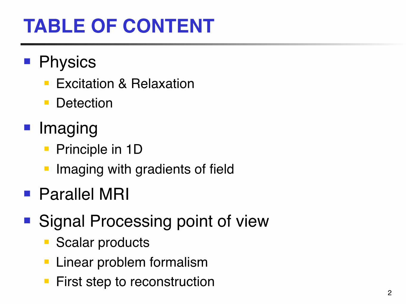
TABLE OF CONTENT
2
Physics Excitation & Relaxation Detection
Imaging Principle in 1D Imaging with gradients of field
Parallel MRI Signal Processing point of view
Scalar products Linear problem formalism First step to reconstruction
Physics
3
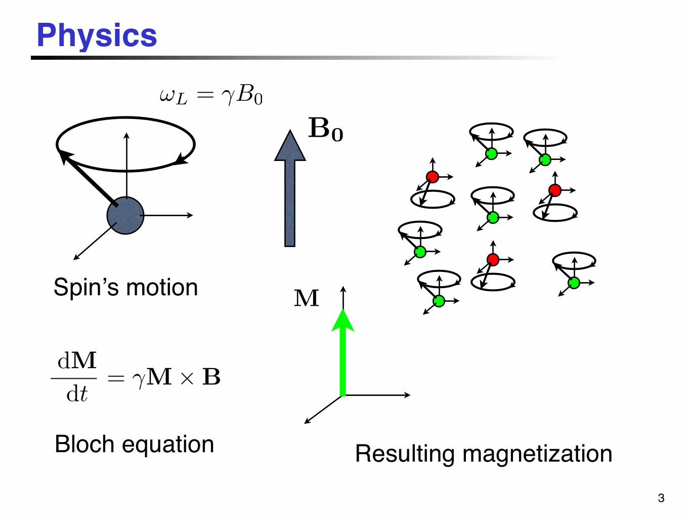
Resulting magnetization
Spinʼs motion
B0
M
dMdt
= !M!B
Bloch equation
!L = "B0
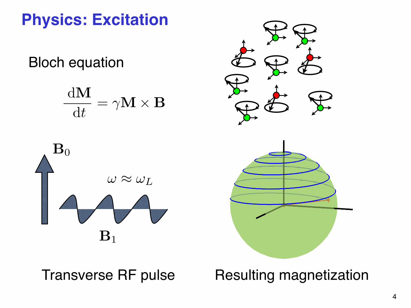
B1
B0
! ! !L
Physics: Excitation
4
Resulting magnetization
dMdt
= !M!B
Bloch equation
Transverse RF pulse

−1 −0.8 −0.6 −0.4 −0.2 0 0.2 0.4 0.6 0.8 1−1
−0.8
−0.6
−0.4
−0.2
0
0.2
0.4
0.6
0.8
1
X−component of the magnetization
Y−co
mpo
nent
of t
he m
agne
tizat
ion
100 200 300 400 500 600 700−1
−0.8
−0.6
−0.4
−0.2
0
0.2
0.4
0.6
0.8
1
time in ps
X−co
mpo
nent
of t
he m
agne
tizat
ion
T2*
63%
0 200 400 600 800 1000 1200 1400 1600 1800 20000
0.1
0.2
0.3
0.4
0.5
0.6
0.7
0.8
0.9
1
time in ps
Z−co
mpo
nent
of t
he m
agne
tizat
ion
T1
63%
Free induction decay
Physics: Relaxation
5
B0
MR detection
6
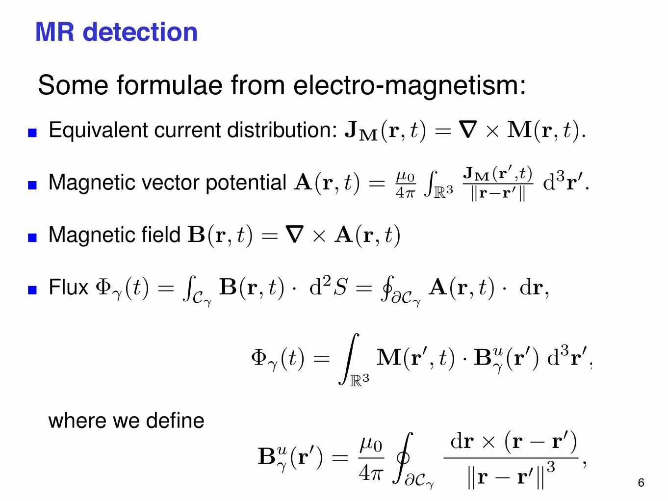
Some formulae from electro-magnetism:Equivalent current distribution: JM(r, t) =!!!"M(r, t).
Magnetic vector potential A(r, t) = µ04!
!R3
JM(r!,t)!r"r!! d3r#.
Magnetic field B(r, t) =!!!"A(r, t)
Flux !"(t) =!C!
B(r, t) · d2S ="
#C!A(r, t) · dr,
!"(t) =#
R3M(r#, t) · Bu
"(r#) d3r#,
where we define
Bu"(r#) =
µ0
4!
$
#C!
dr" (r# r#)$r# r#$3
,

7
MR detection By
Bx
B
I
!!(t) =!
R3M(r!, t) · Bu
!(r!) d3r!Flux
Synchronous demodulation
m!(t) ! !0
!
R3M(r, 0)e!j
R t0 !"(r,#) d#S!(r) d3r
Complex notations:M(r, t) = Mx(r, t) + jMy(r, t) = M(r, 0)e!j
R t0 !(r,") d"
S!(r) = Bu!,x(r)! jBu
!,y(r)
e!(t) = ! d!!
dt(t)
" ! Im!
!0
"
R3M(r, 0)e!j
R t0 "(r,#) d#S!(r) d3r
#Emf
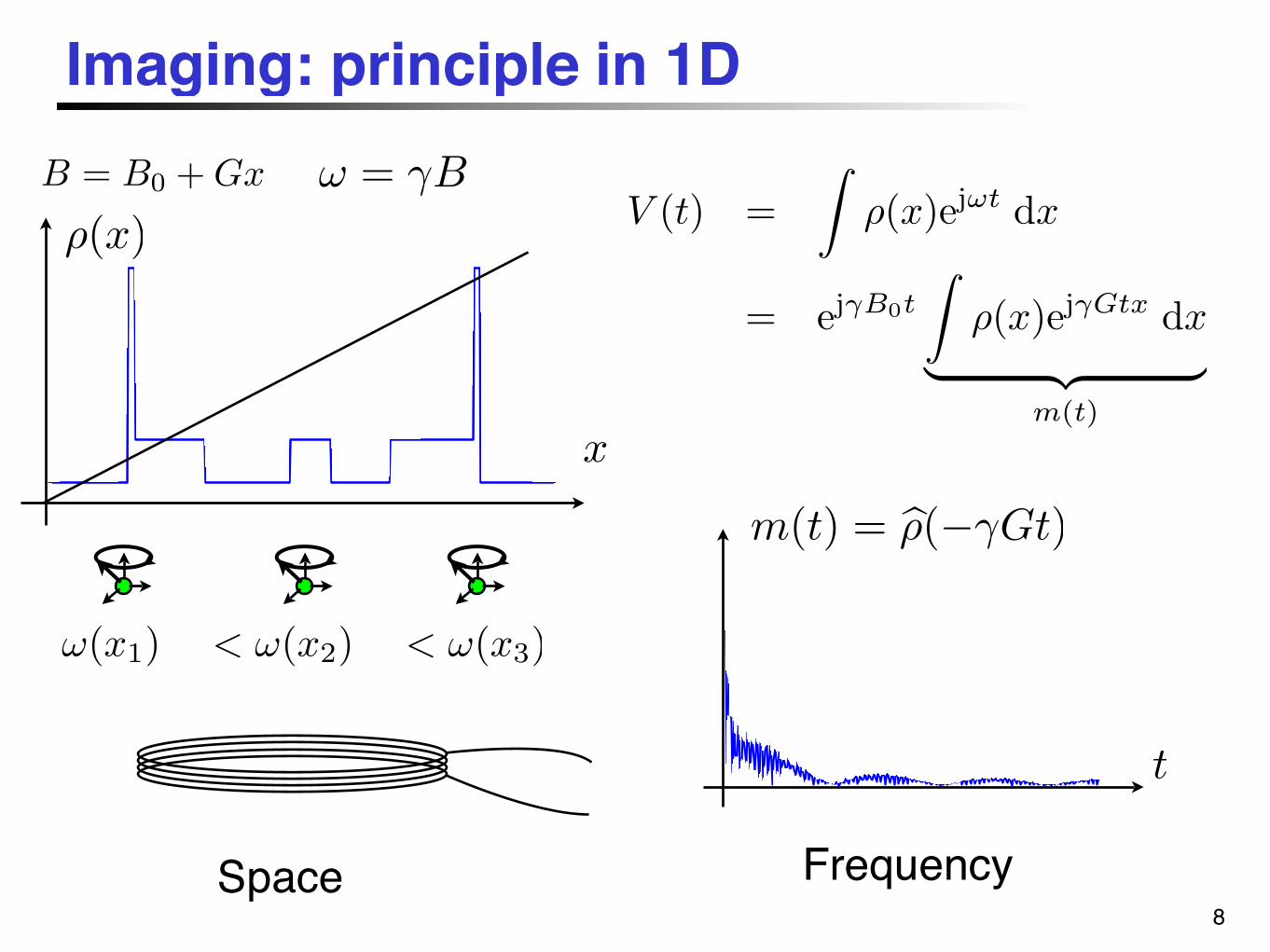
Imaging: principle in 1D
8Space
B = B0 + Gx
x
! = "BV (t) =
!!(x)ej!t dx
= ej"B0t
!!(x)ej"Gtx dx
" #$ %m(t)
Frequency
t
m(t) = !!(!"Gt)
!(x)
!(x1) < !(x2) < !(x3)
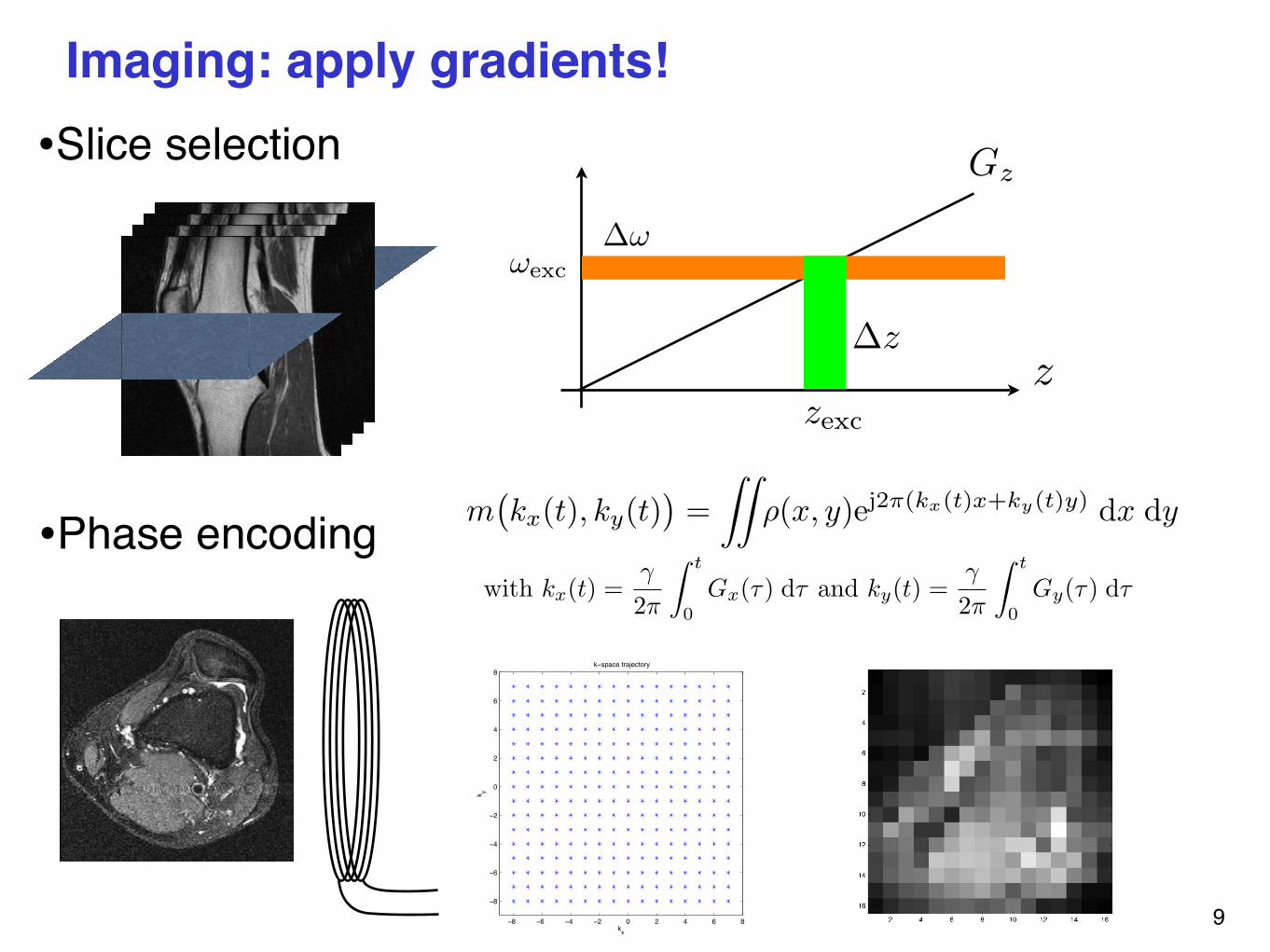
Imaging: apply gradients!
9
z
Gz
!exc
!!
!z
zexc
•Slice selection
•Phase encoding m!kx(t), ky(t)
"=
##!(x, y)ej2!(kx(t)x+ky(t)y) dx dy
with kx(t) =!
2"
! t
0Gx(#) d# and ky(t) =
!
2"
! t
0Gy(#) d#
−8 −6 −4 −2 0 2 4 6 8
−8
−6
−4
−2
0
2
4
6
8 k−space trajectory
kx
k y
10
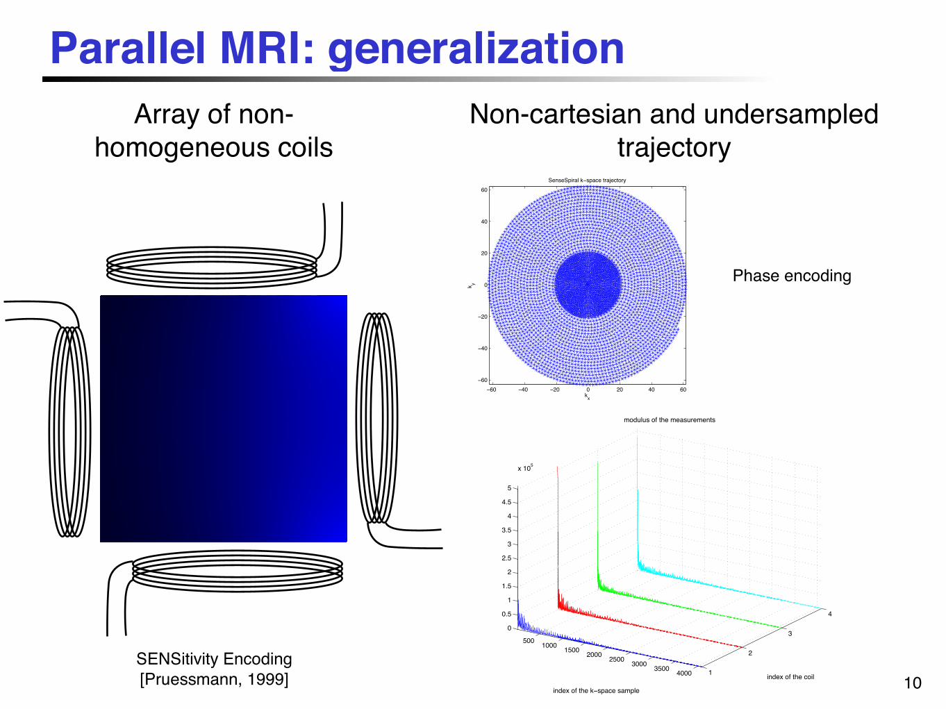
Array of non-homogeneous coils
Non-cartesian and undersampled trajectory
SENSitivity Encoding[Pruessmann, 1999]
Phase encoding
−60 −40 −20 0 20 40 60−60
−40
−20
0
20
40
60
SenseSpiral k−space trajectory
kx
k y
500 1000 1500 2000 2500 3000 3500 4000 1
2
3
4
0
0.5
1
1.5
2
2.5
3
3.5
4
4.5
5
x 105
index of the coil
modulus of the measurements
index of the k−space sample
Parallel MRI: generalization

SP point of view: projection
11
with !!,k(r) = S!!(r)e"2j"k·rm!(k) = !!!,k , ""
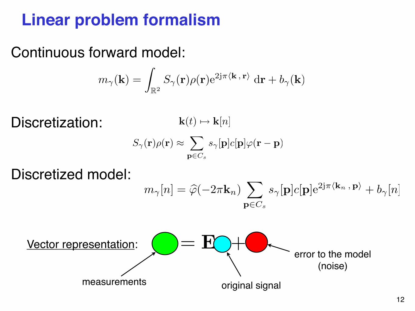
Linear problem formalism
12
Continuous forward model:
Discretization: k(t) !" k[n]
S!(r)!(r) !!
p!Cs
s! [p]c[p]"(r" p)
Discretized model:
m!(k) =!
R2S!(r)!(r)e2j"!k , r" dr + b!(k)
m! [n] = !!(!2"kn)"
p!Cs
s! [p]c[p]e2j""kn , p# + b! [n]
Vector representation: m = Ec + b
measurements original signal
error to the model(noise)

First step to reconstruction
13
Reconstruction often requires the adjoint operator to be computed...
MRI adjoint: MRIH {m!}(r) = S!!(r)
!
Rm!(t)e2j""k(t) , r# dt
MRI measurement followed by adjoint:MRIH MRI{!}(r) = S!
!(r) (g ! S!!) (r)
with g(r) =!
Re2j!!k(t) , r" dt
and "g(!!!) =!
R"(!!! + 2#k(t)) dt

Questions?
14
Thanks for your attention!
Any question?