MR-based pseudo-CT generation using water-fat...

2017

UNIVERSIDADE DE LISBOA

FACULDADE DE CIÊNCIAS

DEPARTAMENTO DE FÍSICA

MR-based pseudo-CT generation using water-fat decomposition

and Gaussian mixture regression

Joaquim Manuel Faria Martins da Costa

Mestrado Integrado em Engenharia Biomédica e Biofísica

Perfil em Radiações em Diagnóstico e Terapia

Dissertação orientada por:

Prof. Dr. Peter Seevinck

Prof. Dr. Alexandre Andrade

i

Resumo

O uso de tomografia computorizada (CT) é considerado como a prática clínica adequada para

aplicações clínicas onde a simulação da atenuação de radiação pelos tecidos corporais é necessária, tais

como a correcção de atenuação dos fotões em Tomografia de Emissão de Positrões (PET) e no cálculo

da dosagem a ser administrada durante o planeamento de radioterapia (RTP).

Imagens de ressonância magnética (MRI) têm vindo a substituir o uso de TC em algumas

aplicações, sobretudo devido ao seu superior contraste entre tecidos moles e ao facto de não usar

radiação ionizante. Desta forma, técnicas como PET-MRI e o planeamento de radioterapia apenas com

recurso a imagens de ressonância magnética são alvo de uma crescente atenção. No entanto, estas

técnicas estão limitadas pelo facto de imagens de ressonância magnética não fornecerem informação

acerca da atenuação e absorção de radiação pelos tecidos.

Normalmente, de forma a solucionar este problema, uma imagem de tomografia computorizada

é adquirida de forma a realizar a correcção da atenuação dos fotões, assim como a dose a ser entregue

em radioterapia. No entanto, esta prática introduz erros aquando do alinhamento entre as imagens de

MRI e CT, que serão propagados durante todo o procedimento. Por outro lado, o uso de radiação

ionizante e os custos adicionais e tempo de aquisição associado à obtenção de múltiplas modalidades de

imagem limitam a aplicação clínica destas práticas.

Assim, o seguimento natural prende-se com a completa substituição do uso de CT por MRI. Desta

forma, o desenvolvimento de um método para a obtenção de uma imagem equivalente a CT usando MRI

é necessário, sendo a imagem resultante designada de pseudo-CT.

Vários métodos foram desenvolvidos de forma a construir pseudo-CT, usando métodos baseados

na anatomia do paciente ou em métodos de regressão entre CT e MRI. No entanto, no primeiro caso,

erros significativos são frequentes devido ao difícil alinhamento entre as imagens em casos em que a

geometria do paciente é muito diferente da presente no atlas. No segundo caso, a ausência de sinal no

osso cortical em MRI, torna-o indistinguível do ar. Sequências que usam um tempo de eco muito curto

são normalmente utilizadas para distinguir osso cortical de ar. No entanto, para áreas com maior

dimensão, como a área pélvica, dificuldades relacionadas com o equipamento e com o ruído limitam a

sua aplicação nestas áreas. Por outro lado, estes métodos utilizam frequentemente diferentes imagens de

MRI de forma a obter diferentes contrastes, aumentando assim o tempo de aquisição das imagens.

Nesta dissertação, é proposto um método para a obtenção de um pseudo-CT baseado na

combinação de um algoritmo de decomposição de água e gordura e um modelo de regressão de mistura

gaussiana para a região pélvica através da aquisição de sequências de MRI convencionais. Desta forma,

a aquisição de diferentes contrastes é obtida por pós-processamento das imagens originais.

Desta forma, uma imagem ponderada em T1 foi adquirida com 3 tempos de eco. Um algoritmo

de decomposição do sinal de ressonância magnética em sinal proveniente de água e gordura foi utilizado,

permitindo a obtenção de duas imagens, cada uma representando apenas o sinal da água e gordura,

respectivamente. Usando estas duas imagens, uma imagem da fracção de gordura em cada voxel foi

também calculada. Por outro lado, usando o primeiro e o terceiro eco foi possível calcular o decaimento

de sinal devido a efeitos relacionados com o decaimento T2*. O método para gerar o pseudo-CT baseia-

ii

se num modelo de regressão duplo entre as variáveis relacionadas com MRI e CT. Assim, o primeiro

modelo aplica-se aos tecidos moles, enquanto que o segundo modelo se aplica aos tecidos ósseos. A

segmentação entre estes tecidos foi realizada através da delineação manual dos tecidos ósseos. No caso

do modelo de regressão para os tecidos moles, o modelo consiste numa regressão polinomial entre as

imagens da fracção de gordura e os valores de CT. A ordem do polinómio usada foi obtida pela

minimização do erro absoluto médio. No caso do modelo de regressão para os tecidos ósseos, um modelo

de regressão de mistura gaussiana foi aplicado usando as imagens de gordura, água, de fracção de

gordura e de R2*. Estas variáveis foram selecionadas, uma vez que estudos prévios correlacionam esta

com a densidade mineral óssea, que por sua vez está relacionada com as intensidades em CT. A

influência de incluir no modelo de regressão informação acerca da vizinhança foi estudada através da

inclusão de imagens do desvio padrão nos 27 voxéis na vizinhança das variáveis previamente incluídas

no modelo. O número de componentes a usar no modelo de regressão de mistura gaussiana foi obtido

através da minimização do critério de Akaike. O pseudo-CT final foi obtido pela sobreposição das

imagens obtidas através do duplo modelo de regressão, seguido da aplicação de um filtro gaussiano com

desvio padrão de 0.5 de forma a mitigar os erros na segmentação dos tecidos ósseos. Este método foi

validado usando imagens da zona pélvica de 6 pacientes usando um procedimento leave-one-out-cross-

validation (LOOCV). Durante este procedimento, o modelo foi estimado através das variáveis de 5

pacientes (imagens de treino) e aplicado às variáveis relacionadas com MRI do paciente restante

(imagem de validação), de forma a gerar o pseudo-CT. Este procedimento foi repetido para todas as

seis combinações de imagens de treino e de validação e os pseudo-CT obtidos foram comparados com

a imagem TC correspondente.

No caso do modelo para os tecidos moles, verificou-se que a utilização de um polinómio de

segundo grau permitia a obtenção de melhores resultados. Da mesma forma, verificou-se que a inclusão

de informação acerca da vizinhança permitia uma melhor estimativa dos valores de pseudo-CT no caso

dos tecidos ósseos. A segmentação dos tecidos ósseos foi considerada adequada uma vez que o valor

médio do coeficiente de Dice entre estes tecidos e o osso em CT foi de 0.91 ±0.02. O valor médio do

erro absoluto entre o pseudo-CT e a correspondente CT para todos os pacientes foi de 37.76±3.11 HU,

enquanto que no caso dos tecidos ósseos o valor foi de 96.61±10.49 HU. Um erro médio de -2.68 ± 6.32

HU foi obtido, denotando a presença de bias no processo. Por outro lado, valores médios de peak-to-

signal-noise-ratio (PSNR) e strucutre similarity índex (SSIM) de 23.92±1.62 dB e 0.91±0.01 foram

obtidos, respectivamente. Os maiores erros foram encontrados no recto, uma vez que o ar não foi

considerado neste método, nas interfaces entre diferentes tecidos, devido a erros no alinhamento das

imagens, e nos tecidos ósseos.

Desta forma, o método de obtenção de um pseudo-CT proposto nesta dissertação demonstrou ter

potencial para permitir uma correcta estimativa da intensidade em CT. Os resultados obtidos

demonstram uma melhoria significativa quando comparados com outros métodos encontrados na

literatura que se baseiam num método relacionado com a intensidade, enquanto que se encontram na

mesma ordem de magnitude de métodos baseados na anatomia do paciente. Para além disso, quando

comparados com os primeiros, este método tem a vantagem de apenas uma sequência MRI ser utilizada,

levando a uma redução no tempo de aquisição e nos custos associados. Por outro lado, a principal

limitação deste método prende-se com a segmentação manual dos tecidos ósseos, o que dificulta a sua

implementação clínica. Desta forma, o desenvolvimento de técnicas de segmentação automáticas dos

tecidos ósseos torna-se necessária, sendo exemplos destas técnicas a criação de um shape model ou

através da segmentação baseada num atlas. A combinação destes métodos com o método descrito nesta

dissertação pode permitir a obtenção de uma alternativa às imagens de CT para o cálculo das doses em

radioterapia e correcção de atenuação em PET-MRI.

iii

Palavras-Chave: Ressonância Magnética, Tomografia Computorizada, pseudo-CT, Decomposição de

água e gordura, Regressão de mistura gaussiana

iv

Abstract

Purpose: Methods for deriving computed tomography (CT) equivalent information from MRI are

needed for attenuation correction in PET-MRI applications, as well as for dose planning in MRI based

radiation therapy workflows, due to the lack of correlation between the MR signal and the electron

density of different tissues. This dissertation presents a method to generate a pseudo-CT from MR

images acquired with a conventional MR pulse sequence.

Methods: A T1-weighted Fast Field Echo sequence with 3 echo times was used. A 3-point water-fat

decomposition algorithm was applied to the original MR images to obtain water and fat-only images as

well as a quantitative fat fraction image. A R2* image was calculated using a mono-exponential fit

between the first and third echo of the original MR images. The method for generating the pseudo-CT

includes a dual-model regression between the MR features and a matched CT image. The first model

was applied to soft tissues, while the second-model was applied to the bone anatomy that were

previously segmented. The soft-tissue regression model consists of a second-order polynomial

regression between the fat fraction values in soft tissue and the HU values in the CT image, while the

bone regression model consists of a Gaussian mixture regression including the water, fat, fat fraction

and R2* values in bone tissues. Neighbourhood information was also included in the bone regression

model by calculating an image of the standard deviation of 27-neighbourhood of each voxel in each MR

related feature. The final pseudo-CT was generated by combining the pseudo-CTs from both models

followed by the application of a Gaussian filter for additional smoothing. This method was validated

using datasets covering the pelvic area of six patients and applying a leave-one-out-cross-validation

(LOOCV) procedure. During LOOCV, the model was estimated from the MR related features and the

CT data of 5 patients (training set) and applied to the MR features of the remaining patient (validation

set) to generate a pseudo-CT image. This procedure was repeated for the all six training and validation

data combinations and the pseudo-CTs were compared to the corresponding CT image.

Results: The average mean absolute error for the HU values in the body for all patients was 37.76±3.11

HU, while the average mean absolute error in the bone anatomy was 96.61±10.49 HU. No large

differences in method accuracy were noted for the different patients, except for the air in the rectum

which was classified as soft tissue. The largest errors were found in the rectum and in the interfaces

between different tissue types.

Conclusions: The pseudo-CT generation method here proposed has the potential to provide an accurate

estimation of HU values. The results here reported are substantially better than other voxel-based

methods proposed. However, they are in the same range as the results presented in anatomy-based

methods. Further investigation in automatic MRI bone segmentation methods is necessary to allow the

automatic application of this method into clinical practice. The combination of these automatic bone

segmentation methods with the model here reported is expected to provide an alternative to CT images

for dose planning in radiotherapy and attenuation correction in PET-MRI.

Keywords: Magnetic Resonance, Computed Tomography, pseudo-CT, water-fat decomposition,

Gaussian mixture regression

v

Acknowledgments

Firstly, I would like to start by thanking my supervisor Peter Seevinck from the University

Medical Center (UMC) Utrecht, who gave me the opportunity to join his research group to perform this

amazing project. During this internship, he was a great motivator, patient and he was always available

to teach me everything that I wanted to know and basically for all the guidance during my stay at UMC

Utrecht. I learned a lot because of him and he was not just a good supervisor but also a great friend. I

have nothing more than absolute respect and admiration for him and I wish him all the best in the world.

I also want to thank Marijn van Stralen who was essential for my work for always being there to help

me and advise me. His expertise, understanding and patience added considerably to my project and I

have the most respect for him and his work and dedication.

I would also like to thank Matteo Maspero and Frank Zijlstra for all the support and great

advises that were essential for a better understanding of this project. Furthermore, a big thanks to Harry

Hu, Chen Cui and Joshua Kim for being available to clarify my doubts about their methods throughout

the project.

A big thank you to everybody in the Image Science Institute from UMC who received me so well

and who made me feel that I was at home every day. A special thanks to Valerio Manippa and Luis

Alberto for being my office buddies, for their friendship and for the great moments and happy times.

I would also like to thank to my supervisor Alexandre Andrade, for all the support and for being

always available to help me regarding the problem! I must also acknowledge the Reitoria da

Universidade de Lisboa for the financial support, under the ERASMUS program, that made this

internship possible.

In addition, a very special thantks to all the people I met in Utrecht, especially Richard Heery,

Hugo Suberbie, Adrien Damseaux and Samuel Bradley for the wonderful adventures we had. Also,

all the people from the Bilstraat family and the UCU guys, you’ll never be forgotten.

To all my friends in Portugal, from Lisbon to Guimarães, from FCUL, to RUEM, passing by

Anexo and finishing in the Arco guys, I could not thank you enough for what you’ve done for me!

Last but not least, there are no words to describe how grateful I am to my wonderful parents

Joaquim and Maria for all the support and for making the person that I am, to my sister and nephew

Marisa and Andre. A big and special thanks to my brother Miguel for all the support and for being

always an example and a tutor for me!

vi

List of Acronyms

2D – Two dimensional

3D – Three dimensional

AIC – Akaike’s Information Criterium

CT – Computed Tomography

dB - Decibel

dUTE – Differential Ultrashort Echo Time

EM – Expectation Maximization

FF – Fat Fraction

FFE – Fast Field Echo

FID – Free Inductive Decay

FOV – Field of View

GE – Gradient Echo

GMM – Gaussian Mixture Model

GMR – Gaussian Mixture Regression

HU – Hounsfield Unit

IDEAL – Iterative Decomposition of Water and Fat with Echo Asymmetry and Least Squares

Estimation

IP – In Phase

ISI – Image Sciences Institute

LOOCV – Leave-One-Out-Cross-Validation

MAE – Mean Absolute Error

ME – Mean Error

mm- millimetre

MR – Magnetic Resonance

MRI – Magnetic Resonance Imaging

ms – millisecond

MSE – Mean Square Error

NMR – Nuclear Magnetic Resonance

NSA – Number of Samples Average

vii

NSSD – Local Sum of Squared Differences

OP – Out of Phase

PD – Proton Density

PET – Positron Emission Tomography

PSNR – Peak Signal-to-Noise Ratio

QSM – Quantitative Susceptibility Mapping

RF - Radiofrequency

ROI – Region of Interest

RTP – Radiotherapy Planning

SE – Spin Echo

SNR – Signal-to-Noise Ratio

SSIM – Structure Similarity Index

STIR – Short-Tau Inversion Recovery

T - Tesla

TE – Echo Time

TR - Repetition Time

UMC – University Medical Centre

UTE – Ultrashort Echo Time

viii

List of Figures

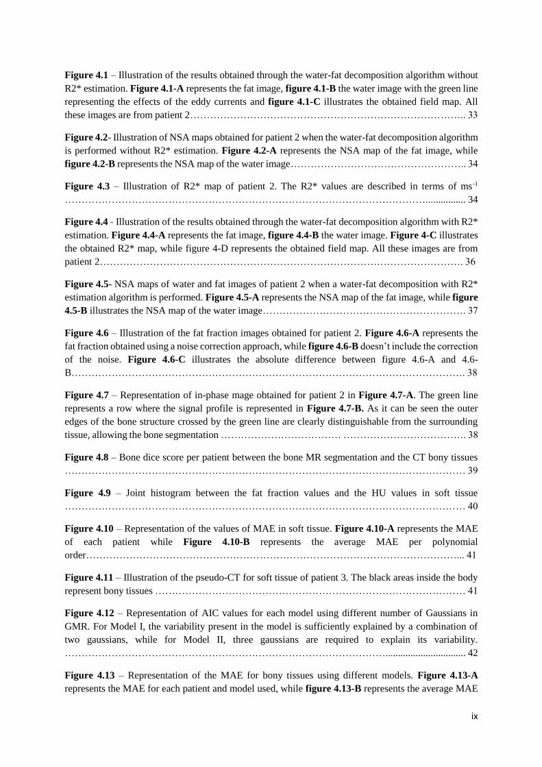
Figure 2.1 - HU values for different tissue types in human body. y-scale represents the HU

scale…………………………………………………………………………………………………….. 4

Figure 2.2 – Illustration of a single particle momentum and resulting magnetization vector when there

is no external force applied. ……………………………………………………………. …………….. 5

Figure 2.3 – Illustration of a single particle momentum and resulting magnetization vector when there

B0 magnetic field is applied……………………………………………………………………………. 6

Figure 1.4 – Illustration of a single particle momentum and resulting magnetization vector when the

RF-pulse (B1 field) is applied ……………………………………………………………. …………… 7

Figure 2.5 – Illustration of the resonance spectrum of water and fat at 3 Tesla. The stars represent the

additional peaks of fat………………………………………………………………………………..... 10

Figure 2.6 – Workflow of an atlas-based approach to generate a pseudo-CT………………………… 15

Figure 2.7 – Several Types of manual bulk density assignment……………………………………… 17

Figure 2.8 – Illustration of the workflow of pseudo-CT generation using a fuzzy c-means algorithm

………………………………………………………………………………………………………… 19

Figure 2.9 - Illustration of GMR using a simple univariate input and output. Left: Data generated by

adding Gaussian noise to 3 linear functions. Middle: A GMM consisting of K=3 components is

estimated using the EM algorithm with K-means initialization, mean values are marked as red dots.

Right: GMR estimation of the expected value of y (green line). ……………………………………. 22

Figure 2.10 – Illustration of GMR using different number of components. Data is the same as in figure

2.9. Left: The GMM has been estimated using 25 components (over-fitting). Right: The GMM has been

estimated using 2 components (under-fitting)………………………………………………………… 23

Figure 3.1- Representation of the derivation of the CT bone binary mask. Figure 3.1-A represents the

CT image. Figure 3.1 -B represents the bone binary mask after the thresholding. Figure 3.1-C

represents the binary mask after the removal of the spurious objects and figure 3.1-D represents the

final bone binary mask after the morphological hole filling operation……………………. ………… 25

Figure 3.2 – Workflow of the masking in MR features………………………………………………. 27

Figure 3.3 – Bone segmentation according the IP image using Mevislab. Purple structures represent the

segmented bony tissues………………………………………………………….................................. 28

Figure 3.4 – Workflow of model selection and pseudo-CT construction in the bone using a GMR

procedure. The left side of the scheme represents the pseudo-CT construction using a model which

doesn´t include neighbourhood information, while in the right side, the workflow of generating a bone

pseudo-CT through a model which includes neighbourhood information is explained……………… 30

Figure 3.5 – Illustration of the workflow to obtain the final pseudo-CT. After estimating the dual-model

regression parameters for soft and bony tissues, the resulting pseudo-CTs were overlapped. After, a

Gaussian filter is applied for smoothing. …………………………………………………..…………. 31

ix

Figure 4.1 – Illustration of the results obtained through the water-fat decomposition algorithm without

R2* estimation. Figure 4.1-A represents the fat image, figure 4.1-B the water image with the green line

representing the effects of the eddy currents and figure 4.1-C illustrates the obtained field map. All

these images are from patient 2……………………………………………………………………….. 33

Figure 4.2- Illustration of NSA maps obtained for patient 2 when the water-fat decomposition algorithm

is performed without R2* estimation. Figure 4.2-A represents the NSA map of the fat image, while

figure 4.2-B represents the NSA map of the water image…………………………………………….. 34

Figure 4.3 – Illustration of R2* map of patient 2. The R2* values are described in terms of ms-1

………………………………………………………………………………………………................ 34

Figure 4.4 - Illustration of the results obtained through the water-fat decomposition algorithm with R2*

estimation. Figure 4.4-A represents the fat image, figure 4.4-B the water image. Figure 4-C illustrates

the obtained R2* map, while figure 4-D represents the obtained field map. All these images are from

patient 2………………………………………………………………………………………………. 36

Figure 4.5- NSA maps of water and fat images of patient 2 when a water-fat decomposition with R2*

estimation algorithm is performed. Figure 4.5-A represents the NSA map of the fat image, while figure

4.5-B illustrates the NSA map of the water image……………………………………………………. 37

Figure 4.6 – Illustration of the fat fraction images obtained for patient 2. Figure 4.6-A represents the

fat fraction obtained using a noise correction approach, while figure 4.6-B doesn’t include the correction

of the noise. Figure 4.6-C illustrates the absolute difference between figure 4.6-A and 4.6-

B………………………………………………………………………………………………………. 38

Figure 4.7 – Representation of in-phase mage obtained for patient 2 in Figure 4.7-A. The green line

represents a row where the signal profile is represented in Figure 4.7-B. As it can be seen the outer

edges of the bone structure crossed by the green line are clearly distinguishable from the surrounding

tissue, allowing the bone segmentation ……………………………… ………………………………. 38

Figure 4.8 – Bone dice score per patient between the bone MR segmentation and the CT bony tissues

………………………………………………………………………………………………………… 39

Figure 4.9 – Joint histogram between the fat fraction values and the HU values in soft tissue

………………………………………………………………………………………………………… 40

Figure 4.10 – Representation of the values of MAE in soft tissue. Figure 4.10-A represents the MAE

of each patient while Figure 4.10-B represents the average MAE per polynomial

order…………………………………………………………………………………………………... 41

Figure 4.11 – Illustration of the pseudo-CT for soft tissue of patient 3. The black areas inside the body

represent bony tissues ………………………………………………………………………………… 41

Figure 4.12 – Representation of AIC values for each model using different number of Gaussians in

GMR. For Model I, the variability present in the model is sufficiently explained by a combination of

two gaussians, while for Model II, three gaussians are required to explain its variability.

……………………………………………………………………………………................................ 42

Figure 4.13 – Representation of the MAE for bony tissues using different models. Figure 4.13-A

represents the MAE for each patient and model used, while figure 4.13-B represents the average MAE

x

using each model for bony tissues HU estimation. As it is possible to see, Model II exhibits superior

predicting performance in terms of MAE for all the patients used in this

study…………………………………………………………………………………………………... 43

Figure 4.14 – Illustration of the pseudo-CT obtained for bony tissues of patient 3…………………. 43

Figure 4.15 – Representation of the obtained pseudo-CTs (first column, figures A, D, G, J, M), the

corresponding CT slices (second column, figures B, E, H, K, N) and the absolute difference between

the pseudo-CT and CT (third column, figures C, F, I, L, O). The first three rows represent transverse

slices for patient 3,5 and 6, respectively. The fourth and fifth rows represent sagittal and coronal slices

from patient 5, respectively. The upper scale bar belongs to the pseudo-CT and the real CT whereas the

lower belongs to the absolute difference images……………………………………………………… 45

Figure 4.16 – Relation between the MAE and the true CT values, showing that the higher the HU, higher

the MAE, excepting for the air (-1000 HU) which was not considered in the soft tissue regression

model………………………………………………………………………………………………….. 46

Figure 4.17 – Mean Absolute Error between the pseudo-CT and CT before and after the application of

the Gaussian filter. Figure 4.17-A represents the MAE in the body for all the patients, while figure

4.17-B represents the MAE in bony tissue for all the

patients……………………………………………… ………………………………………………...46

Figure 4.18-A and figure 4.18-B – Representation of the obtained value for each patient of the SSIM

and the PSNR, respectively, before and after the application of the Gaussian filter ………………… 47

Figure 4.19 – Joint histogram between the true CT number and the predicted CT number. The green

line represents the ideal scenario where the pseudo-CT is exactly equal to the real CT. Points below this

line indicate a higher HU in the real CT compared to the pseudo-CT, while points above indicate a

higher HU in the pseudo-CT compared to the real CT. ………………………………………………. 48

xi

Contents

Resumo ..................................................................................................................................................... i

Abstract .................................................................................................................................................. iv

Acknowledgments ................................................................................................................................... v

List of Acronyms .................................................................................................................................... vi

List of Figures ...................................................................................................................................... viii

1. Introduction ............................................................................................................................... 1

2. Background ............................................................................................................................... 4

2.1. CT imaging .............................................................................................................................. 4

2.2. MR Imaging ............................................................................................................................ 5

2.2.1. Physical Principles .......................................................................................................... 5

2.2.2. Fat and water Magnetic Resonance Imaging ................................................................... 9

2.2.2.1. Physics of water-fat imaging ................................................................................. 10

2.2.2.1.1. NMR Spectrum of water and fat ........................................................................ 10

2.2.2.1.2. B0 Inhomogeneities ............................................................................................ 10

2.2.2.2. Water-Fat Separation Techniques ......................................................................... 11

2.2.2.2.1. Chemical shift based water-fat separation .......................................................... 11

2.2.2.2.1.1. Graph Cut Water-Fat decomposition algorithm .......................................... 12

2.2.2.2.1.2. Fat Fraction ................................................................................................. 14

2.3. Estimating HU values from MR data .................................................................................... 14

2.3.1. Anatomy-based methods ............................................................................................... 15

2.3.1.1. Atlas-based method ............................................................................................... 15

2.3.1.2. Patch-based method ............................................................................................... 16

2.3.2. Voxel-based methods .................................................................................................... 17

2.3.2.1. Manual Bulk Density Assignment ......................................................................... 17

2.3.2.2. Direct Voxelwise Conversion ................................................................................ 17

2.4. Gaussian Mixture Regression ................................................................................................ 20

2.4.1. Gaussian Mixture Model ............................................................................................... 20

2.4.2. Regression using a Gaussian Mixture Model ................................................................ 21

2.4.3. Impact of changing the number of components ............................................................ 22

3. Methods and Materials ............................................................................................................ 24

3.1. Data Specification ................................................................................................................. 24

3.1.1. CT acquisition ............................................................................................................... 24

3.1.2. MR acquisition .............................................................................................................. 24

xii

3.2. MR/CT Registration .............................................................................................................. 24

3.3. Water/Fat Decomposition and R2* estimation ...................................................................... 26

3.4. MR and CT masking ............................................................................................................. 27

3.5. Pseudo-CT generation and Validation................................................................................... 28

3.5.1. MRI bone segmentation ................................................................................................ 28

3.5.2. Soft tissue HU conversion model .................................................................................. 29

3.5.3. HU conversion model for bone anatomy ....................................................................... 29

3.5.4. Final Pseudo-CT generation and metrics of evaluation ................................................. 31

4. Results and Discussion ............................................................................................................. 33

4.1. Water-Fat Decomposition and R2* estimation ...................................................................... 33

4.2. Pseudo-CT generation ........................................................................................................... 39

4.2.1. MRI bone segmentation ................................................................................................ 39

4.2.2. Soft tissue HU conversion model .................................................................................. 39

4.2.3. HU conversion model for bone anatomy ....................................................................... 41

4.2.4. Final pseudo-CT generation and evaluation .................................................................. 43

5. Conclusions and Future Work .................................................................................................. 49

References ............................................................................................................................................. 51

Appendix ............................................................................................................................................... 57

Appendix I ......................................................................................................................................... 57

1

Chapter 1

Introduction

Computed tomography (CT), with its high availability and geometric accuracy, has proven to be

an invaluable tool for many clinical applications where radiation transport simulation is necessary. Since

the voxel’s intensity of a CT image is related to the tissue electron density, CT images may be used to

quantify the attenuation of X-rays within a tissue, which, in turn, is necessary to simulate radiation

transport. For this reason, CT is considered as the golden standard technique of both radiotherapy

planning (RTP) and attenuation correction of Positron Emission Tomography (PET) images [1] [2].

Despite the many advantages of CT, Magnetic Resonance Imaging (MRI) is starting to replace

the use of CT in some applications, mainly due to improved soft tissue contrast and the lack of ionizing

radiation.

PET-MRI is an emerging technology with enormous potential for improvements over PET-CT

for staging, multiparametric therapy planning and functional assessment of treatment response. PET-

MRI was shown to outperform PET-CT in the diagnostic and evaluation of some lesions and diseases,

such as breast cancer, prostate cancer and the detection of soft tissue lesions in the brain, liver and lymph

nodes [3] [4] [5]. However, current PET-MRI systems lack accurate attenuation correction, which is the

most significant of all the corrections applied during PET image reconstruction[6] [7] [8] [9]. Since the MRI

voxel’s intensity is governed by the proton density and relaxation effects, there is no relation between

the MRI voxel’s intensity and the tissue electron density, necessary to perform the attenuation

correction[10].

MR-based RTP and integrated MRI treatment machines, such as MRI linear accelerator

combinations, are another emerging technologies, with the potential to improve tumour visualization

during treatment compared to conventional systems that use ionizing radiation[11] [12] [13]. Several studies

have shown the superiority of MRI for contouring tumour and organs at risk volumes in terms of target

volume delineation[14] [15] [16]. However, similar to the attenuation correction for PET-MRI, radiation

absorption in tissue depends on photon interaction with electrons, and MRI does not directly relate to

such effects.

Traditionally, to overcome these problems, CT is also performed in order to calculate the

attenuation correction map as well as the dose to be delivered. However, this practice introduces

systematic errors in MRI-CT registration, that will cause ambiguities in the following PET-MRI and

MR-RTP procedures. Furthermore, the use of ionizing radiation and the additional costs and scanning

time associated with obtaining and using multiple imaging modalities are serious limitations of this

practice[17].

Thus, the natural follow-up is to completely replace the use of CT by MRI. When residing to

MRI-only techniques, there must be an accurate method to derive CT equivalent data from the MR data

to be able to perform attenuation correction and dose calculations in the same way as it is done when

using a real CT image. MRI-based CT-equivalent images are generally called pseudo-CT images (or

synthetic CT or substitute CT). This approach brings many benefits including the reduction of imaging

2

acquisition costs and radiation exposure, as well as the elimination of the registrations errors between

different imaging modalities[18].

Several methods were developed in order to generate a pseudo-CT, either by using an anatomy-

based approach or a voxel-based approach. The main challenge for the first case lies in the difficulty of

accurate registration when the patient’s geometry is very different from the atlas, which will lead to

significant errors. When using a voxel-based approach, one of the main problems is the lack of signal in

cortical bone, making it indistinguishable from the air[18]. Ultrashort Echo Time (UTE) sequences have

been proposed to distinguish bone and air[19]. However, for areas with a large field of view (FOV), such

as the pelvic area, difficulties related to the hardware and noise considerations associated with UTE

sequences make them unsuitable for clinical application[20]. Furthermore, most of these methods also

acquire different MR sequences in order to obtain different contrasts to generate the pseudo-CT, which

leads to an increase in scanning time[21] [22] [23].

In this dissertation, we propose to develop a MRI conversion approach for the generation of

pseudo-CTs using a combination of an MR-based water-fat decomposition algorithm with a Gaussian

mixture regression algorithm for the pelvic area. In this way, the acquisition of different sequences to

obtain different contrasts will be replaced by contrasts that could be obtained through post-processing

of images from a single acquisition. Specifically, water and fat images may be obtained from a water-

fat-decomposition algorithm. Moreover, other semi-quantitative images may be obtained by the

conjugation of these two images, such as a fat fraction image, that may provide a different contrast

between voxels. Furthermore, as a gradient-echo sequence is used, an estimation of the T2* decay is

possible. In this work, a dual-model regression is applied, with one model applied to soft tissue and the

second model tuned to the bone anatomy obtained by segmentation. As soft tissues are mainly

constituted by water and fat, the use of a water-fat decomposition scheme seems obvious for the

separation of these two species in the MR images, followed by HU values assignment through

regression. Regarding the bone anatomy, it was demonstrated the correlation of the T2* decay as well

as proportion of the fat signal in a voxel with the bone mineral density [17][24] [25] [26] [27]. Furthermore, the

correlation between the HU values and the bone mineral density was also demonstrated, with higher

bone mineral density tissues, normally caused by the presence of minerals such as calcium, representing

denser bones [28]. By including the water and fat information together with information about the T2*

decay in a Gaussian mixture regression procedure, it is expected to obtain a good estimation of the HU

units in the bone anatomy. Also, the influence of including neighbourhood information for HU

estimating in the bone anatomy is investigated. This approach was evaluated on six patient datasets for

which CT and MR images were available for prostate sites, by using a leave-one-out-cross-validation

procedure. The pseudo-CTs were obtained for the six patients and were compared to the corresponding

CT images.

The goal of this project was to investigate if the conversion of MR-data into CT equivalent data

could be established without prior CT information and by a better fundamental understanding of the MR

signal itself, aiming at completely removing CT acquisitions of the traditional workflow of PET-MRI

and MR-RTP.

This dissertation describes the work performed at Image Sciences Institute (ISI), part of the

University Medical Center (UMC) of Utrecht, The Netherlands, during a 10 months internship. The

work is here organized in 5 chapters. Chapter 2 provides background information about CT imaging,

MR imaging and MR-based water-fat decomposition, different approaches to derive a pseudo-CT and

Gaussian mixture regression. Chapter 3 describes the data, software and methods used in this work.

3

Chapter 4 presents the relevant results and also the discussion. Finally, Chapter 5 summarizes the main

conclusions and possible future work.

4

Chapter 2

Background

2.1. CT imaging

In CT, transaxial X-ray projections are computed to create cross-sectional images of the human

body. In a CT scanner, the X-ray tube rotates around the body, while the beams pass through the patient

at different angles. The intensity of the attenuated beams is measured and then converted into an electric

signal using detectors placed on the opposite side of the X-ray tube. After processing, these signals are

transformed into attenuation values consisting of the CT raw data[29]. This data is then converted into an

image using one of several possible a CT reconstruction algorithms, of which the filtered back-

projection algorithm is the most widely used[30]. As a final result, each voxel of the reconstructed CT

image represents a scanned voxel with a specific Hounsfield Unit (HU), describing the degree of

attenuation relative to water[31]:

HU(i, j) = 1000 ×

μ(i, j) − μwμw

(2.1)

where μ(i, j) represents the linear attenuation coefficient of the voxel (i, j) and μw is the linear

attenuation coefficient for water at the same spectrum of photon energies.

The HU is a measure that describes the absorption properties of the tissue relative to water.

Therefore, different HU values are responsible for creating different contrasts in a CT image, as it can

be seen in figure 2.1[31]. Generally, bone appears brighter since it has the highest HU values (ranging

from 400 to 1800 HU), air is black as it presents the smallest HU values (-1000 HU), while soft tissues

present different shades of grey according to their HU values[32] [33]. The similarity in HU values for

different soft tissues makes the distinction between tumours and healthy tissues difficult.

Figure 2.1 - HU values for different tissue types in human body. y-scale represents the HU scale [33].

5

The accuracy of attenuation correction and dose calculations based on CT images is determined

by the precision of HUs to relative electron densities conversion. This relationship is called calibration

curve[34].

2.2. MR Imaging

2.2.1. Physical Principles

Due to the magnetic properties of the atomic nuclei, protons and neutrons present a spin angular

momentum and an associated magnetic moment 𝜇. In Nuclear Magnetic Resonance (NMR), instead of

a single particle, it is important to study all particles[35]. Thus, it is important to convert from the magnetic

momentum of a single particle to a measure that represents the sum of all magnetic momenta. This sum

can be represented by a vector called magnetization, �⃗⃗⃗�:

�⃗⃗⃗� = ∑𝜇𝑖⃗⃗⃗⃗

(2.2)

For NMR’s studies, two components of �⃗⃗⃗� are important: 𝑀𝑥𝑦⃗⃗ ⃗⃗ ⃗⃗ ⃗⃗⃗, the transverse magnetization, and

𝑀𝑧⃗⃗ ⃗⃗⃗⃗ , the longitudinal magnetization. In a state without any external force applied, the magnetic

momentum of each particle is random, and therefore �⃗⃗⃗� is equal to 0, as it can be seen in figure 2.2[35]

[36].

When an external magnetic field B0 is applied (normally in z-component), the magnetic

momentum of each particle will align with the direction of B0, and therefore the magnetization vector

in the z-direction is not 0, as represented in figure 2.3. For 1H, which is the most typical isotope used in

NMR, only two magnetic momenta are allowed (±1/2) and therefore two energy states are allowed,

having the same energy. However, if the proton is placed into B0, the angular momentum will align with

Figure 2.2 – Illustration of a single particle momentum and resulting magnetization vector when there is no external force

applied [36].

6

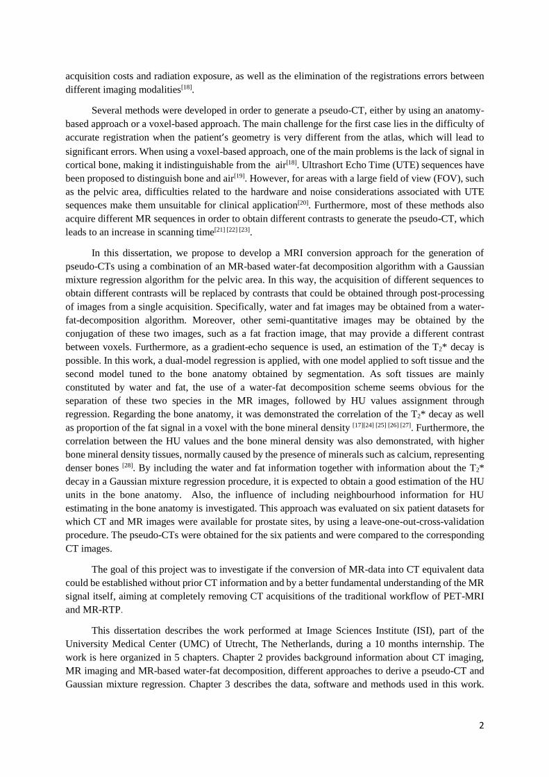
the field direction, making that the resultant magnetic momentum does not have the same energy for

both states. The state with the z-component parallel to B0 presents a lower energy than the state with the

z-component anti-parallel. In this way, there are more particles align parallel to B0 than anti-parallel and

�⃗⃗⃗� will be parallel to B0 [36][37].

It is possible that spin transition from one state to the other one happens by supplying energy to

the system. This energy has to be equal to the difference of energy of both states. This energy supplying

can be done by applying a radio frequency (RF) pulse with frequency equals to

𝜔0 = 𝛾𝐵0 (2.3)

Where 𝜔0 is named Larmor frequency and 𝛾 is the gyromagnetic ratio, that is specific to the used

isotope (for 1H, γ/2π=43 MHz/T).

When the RF pulse (B1 field) is applied in the xy-plane with the Larmor frequency, the particles

in the spin-up state can, therefore, transit to the spin-down state. Adding to this effect, the individual

particles will rotate (precession movement) in phase (phase coherence) allowing a transverse

magnetization to appear, as represented in figure 2.4. Regarding �⃗⃗⃗�, the RF pulse will lead the rotation

of this vector, and the angle of rotation (flip angle, α) will only depend on the amplitude of the B1 field

and the duration of the pulse (t):

𝛼 = 𝛾𝐵1𝑡 (2.4)

Figure 2.3 – Illustration of a single particle momentum and resulting magnetization vector when there B0 magnetic field is

applied [36].

7

As the RF pulse is stopped, the particles return to the rest state as well as �⃗⃗⃗�. For this to happen,

the particles emit a RF wave with the Larmor frequency, called the free inductive decay (FID). The

return to the equilibrium state is called relaxation and is governed by two physical phenomena: spin-

lattice relaxation and spin-spin relaxation[36][37] [38].

As the spins return to the spin-up state, 𝑀𝑧⃗⃗ ⃗⃗⃗⃗ returns to the rest state (spin-lattice relaxation) due to

energy dissipation to the spins’ surroundings. This process is called T1 recovery, described by

𝑀𝑍 = 𝑀0 (1 − 𝑒−𝑡/𝑇1)

(2.5)

Where 𝑀0 is the magnetization at t=0, and T1 is the spin-lattice relaxation time or longitudinal

time.

Moreover, after stimulation, the net magnetization starts to dephase (spin-spin relaxation), due to

the inhomogeneities of B0 and the interaction between the spins. This process is called T2 decay and it

is described by

𝑀𝑥𝑦 = 𝑀𝑥𝑦0 𝑒−𝑡/𝑇2

(2.6)

Where T2 is the spin-spin relaxation time or transverse relaxation time.

Although relaxation is the result of stochastic processes, some deterministic conditions, such as

the inhomogeneity of B0, causes different spins to precess with different resonance frequencies. The B0

inhomogeneities may be caused by the presence of mineral such as iron and calcium, that create

distortion in B0[37]. Thus, the spins will dephase, causing the decay of the total transversal magnetization.

In this way, the effective transversal relaxation time will be referred as T2* and it is defined as

1

𝑇2∗ =

1

𝑇2+1

𝑇2′

(2.7)

Figure 2.4 – Illustration of a single particle momentum and resulting magnetization vector when the RF-pulse (B1 field) is

applied [36].

8

Where T2 is the stochastic contribution and T2’ the deterministic. By definition, T2* is always

shorter than T2.

T1, T2 and T2* relaxation times are dependent on the material composition and consequently also

the acquired NMR signal.

However, as the FID signal quickly vanishes due to the T2* decay, it is difficult to acquire.

Therefore, MRI pulse sequences are used for rephasing the spins. The coherent signal that is emitted

after rephasing is designed by echo. In practice, the pulse sequences are always repeated with a fixed

repetition time (TR) in order to reduce the noise and to achieve different space encoding in the different

repetitions. There are two fundamental types of MR pulse sequences: Spin Echo (SE) and Gradient Echo

(GE) sequences[37]. The remaining developed MR sequences derive in some way from the combination

of the SE and GE sequences.

In a SE sequence, after applying a 90° RF-pulse, the transversal magnetization will decay

exponentially according to T2*, due to differences in the frequency precession of different spins. If a

second RF-pulse with a flip angle of 180° is applied, all spins will rotate 180° around the direction of

the B1 field, causing the inversion of the relative phases of the spins in the transversal plane, while the

longitudinal magnetization continues unchanged. In this way, faster spins that were leading in-phase

will now be lagging in phase. After the 180° pulse, these spins will catch up with the slower spins,

causing the rephasing of the spins. This rephasing results in an echo signal. The time between the 90°

pulse and the emission of the echo is called echo time (TE) [37].

Gradient echo sequences are created using a magnetic field gradient instead of a RF-pulse. After

the excitation pulse, typically smaller than 90°, a gradient is switched on, causing the dephasing of the

spins. Then, the polarity of the gradient is reversed, causing the spins’ rephasing and the formation of

an echo. As the spins’ rephasing occurs only with respect to the gradient, and not to other sources of

dephasing, the signal amplitude is dependent on the T2* decay[37].

This T2* decay can be quantified in GE sequences using:

1

𝑇2∗ = 𝑅2

∗ = −log 𝑆(𝑇𝐸𝑛) − log 𝑆(𝑇𝐸1)

𝑇𝐸𝑛 − 𝑇𝐸1

(2.8)

where 𝑆(𝑇𝐸𝑛) is the signal intensity when the TE was equal to the nth echo of the acquisition,

𝑇𝐸𝑛 is the echo time of the nth echo of the acquisition. 𝑆(𝑇𝐸1) is the signal intensity of the first echo of

the acquisition acquired at 𝑇𝐸1.

In this way, MR intensities can be correlated with proton densities, which are related to the

number of hydrogen atoms in a volume, and tissue relaxation properties rather than with the attenuation

properties of the tissues such as in CT. The density and relaxation time of protons in different tissues is

used to create the required contrast and signal intensity for diagnostic purpose in MR images by changes

in TE and TR. The contrasts are created based on a linear look up table, where magnitudes of the

measured signals are converted to a grey tone.

Thus, there are 3 different types of contrasts in MR images that can be created by changing TE

and TR: T2-weighted images, T1- weighted images and proton-density (PD) weighted images[39]. In T2-

weighted images, the TR and TE are both long and tissues with long T2, such as fluids, present the

highest signal intensities, producing a bright appearance. T2 images are often called as “pathology

images” as the abnormal fluids appear bright against the dark normal tissue. In T1-weighted images,

long T1 tissues give the weakest signal and appear dark, as fluids, and bright pixels are associated with

9

short T1 values, such as fat based tissues. This contrast can be achieved by using short TR and TE. T1

images are often called anatomy scans as they display clearly the boundaries between different tissues.

PD-weighted images give a quantitative summary of the number of protons per unit tissue. The higher

the number of protons in a tissue, the brighter the tissue will appear on the image. This contrast can be

achieved by using a long TR and a short TE[39].

As for CT, MRI generates cross-sectional images of the human body. The RF pulse is therefore

delivered only to the slice that is needed to be imaged. Slice position will be selected according to the

central frequency of the applied RF pulse. After selecting slice thickness and position, the spatial

position of the MR signal needs to be identified which is accomplished using spatial encoding. Spatial

encoding comprises two steps, phase encoding and frequency encoding, requiring the application of

additional gradients that will change the magnetic field strength along the x and y axis enabling unique

spatial identification of each voxel. The raw-data space which is used to store the digitized MR signals

during acquisition is called k-space. The k-space has two axes with the horizontal axis (kx) representing

the frequency information and the vertical axis (ky) the phase information. The final MR image will be

created from the raw data by applying the 2D- Fourier Transformation to the k-space after the scan is

over[39].

2.2.2. Fat and water Magnetic Resonance Imaging

Most clinical magnetic resonance imaging applications detect the signal from protons, which

compromise over 90% of nuclei in the human body. The detected protons are either part of water, bound

to molecules or carbohydrates, or fat. Their respective signal intensities in imaging voxels results from

a combination of their spin density, longitudinal and transverse relaxation times (T1 and T2,

respectively), and the parameters of the imaging sequence used. By exploiting the particular

characteristics of hydrogen, MRI can provide excellent contrast between soft tissue, according to

whether they are bound to water or lipid molecules[40].

With its relatively short T1 relaxation time, fat signal often appears bright in many important

clinical imaging sequences and can obscure underlying pathology such as edema, inflammation, or

enhancing tumours. For this reason, water-fat decomposition methods are necessary to supress or detect

fat signal and improve visualization of these abnormalities[40].

Several techniques of water-fat decomposition were proposed such as the chemical shift

saturation pulse and the short-tau inversion recovery (STIR). In the first technique, a frequency selective

RF pulse and a spoiler gradient pulse are used in conjunction to first excite and then saturate the fat

magnetization before water is excited during imaging[41]. In STIR, the longitudinal magnetization of fat

is first flipped 180° by an inversion pulse and then allowed to relax back to its equilibrium along the

magnetic field direction. Water magnetization, which is usually also flipped 180° by the same inversion

pulse, is excited when the longitudinal magnetization of fat crosses the null point. Due to the short T1

relaxation time of fat, water has usually relaxed only partially along the longitudinal axis at the time of

excitation[42] [43].

Although the previous techniques can obtain a reliable fat suppression, for pseudo-CT generation

purposes, detection rather than suppression is more valuable, once quantification of water and fat is

necessary, since they present different HU values, as it can be seen in figure 2.1. Also, it was

demonstrated that the quantitative fat fraction is correlated with bone mineral density, which is

correlated with the HU values of bone[26] [28].

10

In this way, methods that could quantify the signal of water and fat are preferred over suppression

techniques. These methods that are able to perform separation as well as quantification are referred as

chemical shift water-fat decomposition techniques[40] [44].

2.2.2.1. Physics of water-fat imaging

2.2.2.1.1. NMR Spectrum of water and fat

The electronic shielding of the protons in fat molecules is greater than that experienced by protons

in water molecules, resulting in different microscopic magnetic fields, and subsequently different proton

resonance frequencies. Fat has a complex spectrum with multiple peaks, the largest of which is shifted

downfield by ≈ 3.5 ppm from the water peak[40] [45].

The resulting chemical shift, Δfcs in the resonance frequency is linearly related to the magnetic

field strength B0:

∆𝑓𝑐𝑠 =𝛾

2𝜋𝐵0 × ∆𝛿 [𝑝𝑝𝑚] ×10

−6

(2.9)

As the chemical shift is directly proportional to B0, the chemical shift at 1.5 T is -210 Hz (fat

precesses slower than water), while at 3 T, it doubles to -420 Hz at body temperature (37°C), as

represented in figure 2.5[46].

2.2.2.1.2. B0 Inhomogeneities

Most of the water-fat separation techniques rely on the assumption that there are constant

frequencies for fat and water across the image. However, in practical applications many factors can

create inhomogeneities in the B0 field that violate this assumption and result in imperfection suppression

of fat[40].

Although the main magnet itself may have an imperfect magnetic homogeneity, this is a minor

effect since modern MR scanners are shimmed to homogeneity within 1 ppm across the field of view

(FOV). Magnetic susceptibility introduced by the patient leads to more significative B0 inhomogeneities

and it can be caused by several sources, such as air/tissue interfaces, ears or the bowel gas. These B0

Figure 2.5 – Illustration of the resonance spectrum of water and fat at 3 Tesla. The stars represent the additional peaks of

fat [40].

11

inhomogeneities have three main effects: distortion in the readout gradient, accelerated T2* decay for

gradient echo imaging and failed fat suppression which is the most relevant for the context of this

work[40].

2.2.2.2. Water-Fat Separation Techniques

2.2.2.2.1. Chemical shift based water-fat separation

Chemical shift based water-fat separation methods comprise a class of approaches commonly

known as “Dixon” water-fat separation. As for the frequency selective approach, the Dixon techniques

rely on the water-fat chemical shift difference. However, the Dixon techniques encode the chemical shift

difference into the signal difference with a modified data acquisition and then achieve the water/fat

separation through post-processing. In its original approach, Dixon acquired an image with water and

fat signal in-phase and another image with the signal 180° out-of-phase[44] [47]. The choice of the echo

times to achieve these two images is done using

𝑇𝐸 =

𝜃

2𝜋 ∆𝑓𝑐𝑠

(2.10)

where θ is the phase shift between water and fat signal. In this way, the Dixon technique can be

described by the following equation system:

{𝐼𝑃 = 𝑊 + 𝐹𝑂𝑃 = 𝑊 − 𝐹

<=> {𝑊 =

(𝐼𝑃 + 𝑂𝑃)

2

𝐹 =(𝐼𝑃 − 𝑂𝑃)

2

(2.11)

where IP represents the in-phase image, OP the out-of-phase image, F the fat image and W the

water image. As this approach only requires two images, it is considered a “two-point” method.

Unfortunately, Dixon’s original approach was sensitive to B0 inhomogeneities that resulted in

water-fat swapping in the image[40]. Thus, this approach was subsequently modified to include a third

image that was used to compensate for B0 inhomogeneities. This three-point method acquire images at

TE values that generate phase shifts of 0, +π and -π between the water and fat[48]. The additional

information can be used to calculate a B0 field inhomogeneity map (field map). By using phase

unwrapping algorithms, this approach is able to remove the effects of field distortions, thereby avoiding

water-fat swapping, turning this method more robust[44] [49] [50]. However, this technique increases the

scan time and doesn’t allow flexibility in the sequence design since the images have to be acquired at

specific TE values[40].

To allow more flexibility in the pulse sequence design and, consequently, reduce the scan time,

several methods were developed that allow arbitrary TE values to accomplishing the water-fat

separation, such as the iterative decomposition of water and fat with echo asymmetry and least squares

estimation (IDEAL)[51]. This method uses images acquired at arbitrary TE values together with an

iterative least square estimation of the field map to accomplish a voxel-independent water-fat separation.

However, in areas with severe field inhomogeneities this method still fails to obtain an accurate field

map since, with this technique, the field map can be directly estimated only if the true field map ranges

between ± Δfcs/2. In practice, the field inhomogeneity may exceed this range[52]. Furthermore, these

techniques normally use an alternating bipolar readout gradient to achieve scan efficiency and reduce

12

the echo spacing. The use of this alternating bipolar gradient turns the estimation of the field map

susceptible to eddy-currents, which manifest itself as phase errors[53] [54] [55].

More recently, a water-fat separation method that uses a graph-cut algorithm to jointly estimate

water/fat images and the field map was proposed[56]. In this approach, the estimation of the field map at

all voxels is formulated as the minimization of a global criterion, which is the linear combination of the

sum of the voxel-independent criteria and a field map smoothing penalty, and solve it using an iterative

graph cut algorithm. This algorithm is further explained below.

2.2.2.2.1.1. Graph Cut Water-Fat decomposition algorithm

The graph cut water-fat estimation algorithm uses a multi-echo water and fat decomposition

scheme, where a sequence of images is collected with different echo time shifts, t1, t2, tn. The signal at

each individual voxel is described by the following model[51] [56]:

𝑠(𝑟, 𝑡𝑛) = (𝜌𝑤𝑎𝑡𝑒𝑟(𝑟) + 𝜌𝑓𝑎𝑡(𝑟)𝑒𝑗2𝜋∆𝑓𝑐𝑠𝑡𝑛)𝑒−𝜑(𝑟)𝑡𝑛 , 𝑛 = 1,… , 𝑁 (2.12)

where ρwater(r) and ρfat(r) are complex-valued concentrations of water and fat, respectively. The

field map, f(r), is consolidated in 𝜑(𝑟) through

𝜑(𝑟) = [𝑗2𝜋 f(𝑟)]

(2.13)

From this signal model, it is possible to observe that there are 2 complex unknows, ρwater(r) and

ρfat(r), and 1 real unknown, f(r), in a total of 5 (each complex unknown has a real and imaginary

unknown). As each image contributes with a real and imaginary measurement, constituting two

measurements per TE value, at least 3 images at different TE values have to be acquired, since the

number of measurements has to be always equal or higher than the number of unknown parameters.

Also, in this signal model, it is assumed that fat only presents a single resonance frequency.

However, fat has several peaks. In particular, the spectral peak from olefinic proton (5.3 ppm) is close

to the water resonance frequency, which can cause some water-fat swapping[57]. One possible solution

is to include in the signal model a weighted sum of the amplitudes of the fat peaks, by changing equation

2.12 to:

𝑠(𝑟, 𝑡𝑛) = (𝜌𝑤𝑎𝑡𝑒𝑟(𝑟) + 𝜌𝑓𝑎𝑡(𝑟) [∑𝛽𝑖𝑒𝑗2𝜋∆𝑓𝑐𝑠𝑖𝑡𝑛

𝑀

𝑖=1

]) 𝑒−𝜑(𝑟)𝑡𝑛 , 𝑛 = 1,… , 𝑁

(2.14)

Here, the fat signal is modelled using an M (usually 6) peak model, where ∆𝑓𝑐𝑠𝑖 is the chemical

shift between the ith fat peak and water (Hz), and βi >0 is the relative weight of each peak. However, this

model would require N ≥ M+2 images to estimate the unknown parameters, which is not practical due

to the increased scan time. In this way, it is assumed that βi are known. Thus, the number of unknown

parameters remains the same as the single peak model[56] [57]. Consequently, only 3 images have to be

acquired.

However, this multi-peak signal model doesn’t account for T2* decay. Although for many

applications the T2* decay may be neglected, for imaging with substantially shortened T2*, it is

important to consider the effects from both fat and T2*, as they may interfere with the estimation of each

other. Therefore, it is possible to estimate the R2* map, i.e. R2* =1/ T2*, by including it in the signal

13

model[57] [58]. This can be done by modelling the B0 field inhomogeneity and the T2* decay in a complex

field map term, by changing equation 2.13 to:

𝜑(𝑟) = [1 𝑇2∗(𝑟)⁄ − 𝑗2𝜋𝑓(𝑟)]

(2.15)

In this way, the number of unknown parameters increases to 6, thus 3 images acquired at different

TE values should be enough for obtaining all the unknown parameters. However, as the number of

complex acquired images is equal to the number of unknown parameters, the estimation can be very

sensitive to noise. For a better performance, typically 6 echoes are acquired. Furthermore, for pseudo-

CT generation, besides the importance of the R2* estimation for water-fat decomposition, some studies

prove the correlation between R2* values and HU values, especially in bone tissues. This is mainly due

to the correlation between R2* values and bone mineral density, since bone minerals as calcium create

local inhomogeneities that are reflected by R2* values [27].

The model in equation 2.14 can be written in a matrix form as:

[ 𝑒−(𝜑(𝑟)𝑡1) 𝑒−(𝜑(𝑟)𝑡1) (∑𝛽𝑖𝑒

−𝑗2𝜋𝛿𝑖𝑡1

𝑀

𝑖=1

)

𝑒−(𝜑(𝑟)𝑡𝑛) 𝑒−(𝜑(𝑟)𝑡𝑛) (∑𝛽𝑖𝑒−𝑗2𝜋𝛿𝑖𝑡𝑛

𝑀

𝑖=1

)]

⏟ 𝐴𝜑

∗ [𝜌𝑤𝑎𝑡𝑒𝑟𝜌𝑓𝑎𝑡

]⏟

𝑔

= [𝑠[1]

𝑠[𝑁]]

⏟ 𝑠

(2.16)

The unknown parameters are obtained by minimizing the least-square errors between the model

and the measured data:

{𝜌𝑤𝑎𝑡𝑒𝑟 , 𝜌𝑓𝑎𝑡 , 𝜑} = arg min𝜌𝑤𝑎𝑡𝑒𝑟,𝜌𝑓𝑎𝑡,𝜑

‖𝐴𝜑𝑔 − 𝑠‖2 (2.17)

Since the above minimization is dependent on many parameters, the criterion is minimized with

respect to some variables by assuming the other to be fixed, thus eliminating them from the

optimization[59]. Minimizing the above cost function with respect to the concentrations, assuming ϕ to

be fixed, we obtain the optimal concentration estimates as 𝑔𝑜𝑝𝑡 = (𝐴𝜑𝑇𝐴𝜑)

−1𝐴𝜑𝑇 𝑠. Replacing the

optimal concentrations back in the previous cost function, and solving for ϕ, we obtain

𝜑(𝑟) = argmin

𝜑‖𝐴𝜑(𝐴𝜑

𝑇𝐴𝜑)−1𝐴𝜑𝑇 𝑠(𝑟) − 𝑠(𝑟)‖⏟

𝐶(𝑟,𝜑)

2

(2.18)

In case of necessity of R2* estimation, again it is possible to minimize the expression with respect

to T2* to obtain a cost function that is only dependent on f:

𝑓(𝑟) = argmin𝑓min𝑇2∗𝐶(𝑟, 𝜑)

⏟ 𝐷(𝑟,𝑓)

(2.19)

Since the estimation of T2* values doesn’t suffer from ambiguities, an exhaustive search over

possible T2* values can be performed to obtain D from C.

14

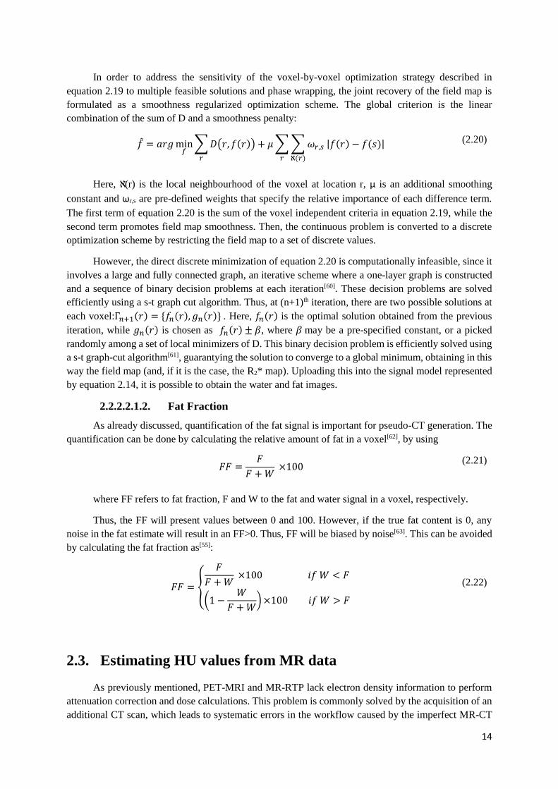
In order to address the sensitivity of the voxel-by-voxel optimization strategy described in

equation 2.19 to multiple feasible solutions and phase wrapping, the joint recovery of the field map is

formulated as a smoothness regularized optimization scheme. The global criterion is the linear

combination of the sum of D and a smoothness penalty:

𝑓 = 𝑎𝑟𝑔min𝑓∑𝐷(𝑟, 𝑓(𝑟))

𝑟

+ 𝜇∑∑𝜔𝑟,𝑠 |𝑓(𝑟) − 𝑓(𝑠)|

ℵ(𝑟)𝑟

(2.20)

Here, ℵ(r) is the local neighbourhood of the voxel at location r, μ is an additional smoothing

constant and ωr,s are pre-defined weights that specify the relative importance of each difference term.

The first term of equation 2.20 is the sum of the voxel independent criteria in equation 2.19, while the

second term promotes field map smoothness. Then, the continuous problem is converted to a discrete

optimization scheme by restricting the field map to a set of discrete values.

However, the direct discrete minimization of equation 2.20 is computationally infeasible, since it

involves a large and fully connected graph, an iterative scheme where a one-layer graph is constructed

and a sequence of binary decision problems at each iteration[60]. These decision problems are solved

efficiently using a s-t graph cut algorithm. Thus, at (n+1)th iteration, there are two possible solutions at

each voxel:Γ𝑛+1(𝑟) = {𝑓𝑛(𝑟), 𝑔𝑛(𝑟)} . Here, 𝑓𝑛(𝑟) is the optimal solution obtained from the previous

iteration, while 𝑔𝑛(𝑟) is chosen as 𝑓𝑛(𝑟) ± 𝛽, where 𝛽 may be a pre-specified constant, or a picked

randomly among a set of local minimizers of D. This binary decision problem is efficiently solved using

a s-t graph-cut algorithm[61], guarantying the solution to converge to a global minimum, obtaining in this

way the field map (and, if it is the case, the R2* map). Uploading this into the signal model represented

by equation 2.14, it is possible to obtain the water and fat images.

2.2.2.2.1.2. Fat Fraction

As already discussed, quantification of the fat signal is important for pseudo-CT generation. The

quantification can be done by calculating the relative amount of fat in a voxel[62], by using

𝐹𝐹 =

𝐹

𝐹 +𝑊 ×100

(2.21)

where FF refers to fat fraction, F and W to the fat and water signal in a voxel, respectively.

Thus, the FF will present values between 0 and 100. However, if the true fat content is 0, any

noise in the fat estimate will result in an FF>0. Thus, FF will be biased by noise[63]. This can be avoided

by calculating the fat fraction as[55]:

𝐹𝐹 = {

𝐹

𝐹 +𝑊 ×100 𝑖𝑓 𝑊 < 𝐹

(1 −𝑊

𝐹 +𝑊)×100 𝑖𝑓 𝑊 > 𝐹

(2.22)

2.3. Estimating HU values from MR data

As previously mentioned, PET-MRI and MR-RTP lack electron density information to perform

attenuation correction and dose calculations. This problem is commonly solved by the acquisition of an

additional CT scan, which leads to systematic errors in the workflow caused by the imperfect MR-CT

15

registration. Thus, the estimation of HU values from MR data is a crucial step in PET-MRI and MR-

RTP workflow.

Several approaches were developed to solve this problem. It is possible to group the several

approaches into two main groups: anatomy-based approaches and voxel-based approaches[18]. The

anatomy-based method generally uses a non-rigid registration between a library of MR reference images

and a new patient MRI to warp a reference CT to match the anatomy of the new patient data[64] [65] [66]

[67]. This method leads to significant errors when the new patient MRI geometry is very different

compared to the geometry of the MR atlas[18]. The voxel-based method could be divided into two types.

The first one involves a direct characterization into different tissue classes by manual segmentation

followed by bulk assignments of HU values[68] [69]. The second one comprises a direct conversion of

MRI voxels values to HU values by introducing a prior correlation between MRI and CT [17] [22] [23] [70]

[71].

2.3.1. Anatomy-based methods

The anatomy-based method could be divided into two main approaches: the atlas-based method[64]

[65] [66] [66] and the patch-based method[72].

2.3.1.1. Atlas-based method

The atlas-based method uses information from the whole image and can be divided in 3 steps, as

illustrated in figure 2.6:

1. First, every CT and MR image from the atlas dataset are aligned using non-deformable

registration (elastic deformation) to enable intra-subject alignment and producing multiple conjugated

CT-MR atlas image pairs[64] [66].

2. Then, a registration between all MR atlas images and the MRI of a new patient is performed

using non-deformable and deformable transformations, enabling the alignment between the MRI of the

new patient and the MR atlas[64] [65].

3. The transformation matrices and deformation fields used in step 2 are also applied to the CT

images in the atlas, building the pseudo-CT, according to different strategies of atlas fusion for HU value

assignment [64] [65].

Figure 2.6 – Workflow of an atlas-based approach to generate a pseudo-CT [64].

16

The HU value for each voxel in the obtained pseudo-CT can be obtained using a simple mean

process[64] [66] or a weighted average based on similarity measures[67].

Using a simple mean process, the pseudo-CT intensity (μ) of a voxel at the position x0 is calculated

using the mean of those at the same location in all deformed CT images in the CT atlas[64]:

𝜇(𝑥0) =1

𝑁𝑎×∑𝑦𝑖(𝑥0)

𝑁𝑎

𝑖=1

(2.23)

Where Na is the number of atlases and yi the HU value in all CT images in the atlas.

In the weighted average based on similarity measures method, the MRI of the new patient is

matched with the MRI atlas database using deformable registration and local image similarity measures

such as the local sum of squared differences (NSSD) and the structural similarity index extended to

regions of interest (ROI-SSIM). The similarity results are ranked across all MR images in the atlas

according to the quality of the registration. The ranks in each nth subject and each voxel �⃗�, 𝑅𝑛�⃗⃗�, are then

converted to weights, 𝑊𝑛�⃗⃗�. Better registration results lead to a higher weight by applying a negative

exponential decay function[67]:

𝑊𝑛�⃗⃗� = 𝑒−𝛽×𝑅𝑛�⃗⃗⃗� (2.24)

Where β is a constant weighting factor. Then the intensity at each voxel of the pseudo-CT is

calculated using

𝐼�⃗⃗�𝑝𝐶𝑇

=∑ 𝑊𝑛�⃗⃗�×𝐽𝑛�⃗⃗�

𝐶𝑇𝑁𝑎𝑛=1

∑ 𝑊𝑛�⃗⃗�𝑁𝑎𝑛=1

(2.25)

Where 𝐽𝑛�⃗⃗�𝐶𝑇 is the atlas CT image from subject n at voxel �⃗�.

2.3.1.2. Patch-based method

The patch-based method involves the use of a rigidly aligned CT-MRI atlas as database but it

excludes the use of deformable registrations. In this method, 3D patches are extracted from the target

MRI followed by a spatial local search of the most intensity similar patches in the MRI database[72].

Thus, the use of deformable registrations is replaced by the patch resemblance search.

The patches extracted from the MRI atlas are centred on an arbitrary spatial location x, PS(x), and

the HU value on position x in the aligned CT is designed by TS(x). Then, using this database, an intensity

based nearest neighbour search is performed using:

𝑑(𝑠, 𝑥) = ‖𝑃(𝑦) − 𝑃𝑆(𝑥)‖2

(2.26)

where P(y) represents the patch at the target MRI. Then, the search is done aiming at finding the

patch that minimizes 𝑑(𝑠, 𝑥). After this search, the corresponding HU value in the CT atlas at the same

spatial location is stored as 𝑇𝑠𝑘𝑚𝑖𝑛(𝑥𝑘𝑚𝑖𝑛). Then, the HU value in the pseudo-CT at position y is

calculated using a weighted average:

𝑝𝐶𝑇(𝑦) =

∑ 𝑤𝑘×𝑇𝑠𝑘𝑚𝑖𝑛(𝑥𝑘𝑚𝑖𝑛)𝑘

∑ 𝑤𝑘𝑘

(2.27)

17

Where the weights, 𝑤𝑘, are calculated by:

𝑤𝑘 = exp(

−𝑑(𝑠𝑘𝑚𝑖𝑛, 𝑥𝑘

𝑚𝑖𝑛

min𝑘𝑑(𝑠𝑘

𝑚𝑖𝑛, 𝑥𝑘𝑚𝑖𝑛

)

(2.28)

2.3.2. Voxel-based methods

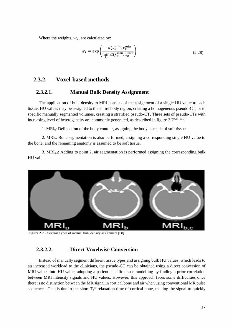
2.3.2.1. Manual Bulk Density Assignment

The application of bulk density to MRI consists of the assignment of a single HU value to each

tissue. HU values may be assigned to the entire body region, creating a homogeneous pseudo-CT, or to

specific manually segmented volumes, creating a stratified pseudo-CT. Three sets of pseudo-CTs with

increasing level of heterogeneity are commonly generated, as described in figure 2.7[68] [69]:

1. MRIu: Delineation of the body contour, assigning the body as made of soft tissue.

2. MRIb: Bone segmentation is also performed, assigning a corresponding single HU value to

the bone, and the remaining anatomy is assumed to be soft tissue.

3. MRIb,c: Adding to point 2, air segmentation is performed assigning the corresponding bulk

HU value.

2.3.2.2. Direct Voxelwise Conversion

Instead of manually segment different tissue types and assigning bulk HU values, which leads to

an increased workload to the clinicians, the pseudo-CT can be obtained using a direct conversion of

MRI values into HU value, adopting a patient specific tissue modelling by finding a prior correlation

between MRI intensity signals and HU values. However, this approach faces some difficulties once

there is no distinction between the MR signal in cortical bone and air when using conventional MR pulse

sequences. This is due to the short T2* relaxation time of cortical bone, making the signal to quickly

Figure 2.7 – Several Types of manual bulk density assignment [68]

18

disappears, and the low proton density of air. Thus, both areas appear as dark in a MRI. To overcome

this problem, UTE sequences were developed[19].

In UTE imaging, the signal is sampled during the FID, allowing the acquisition of the MR signal

in the cortical bone before the signal vanishes. Thus, this pulse sequence uses TEs ranging between

0.008 ms and 0.15 ms, being 10 to 200 times shorter than conventional sequences, by using a hard-

rectangular RF pulse with a small flip angle in combination with a radial, center-out k-space sampling.

Here, the FID is mainly proton-density weighted, lack soft tissue contrast, but providing contrast

between bone and air. In order to obtain more soft tissue contrast, the acquisition of another echo is

needed. The addition of a new echo to the pulse sequence followed by its image subtraction from the

first echo is called differential UTE (dUTE) imaging, enabling the distinction between short T2* species

(bone and air) and long T2* species[25].

For the generation of pseudo-CTs using UTE sequences, automatic segmentation using bulk

density assignment [25] or continuous model based methods may be used[17] [22] [23] [70] [71].

Regarding the bulk density assignment, a pseudo-CT may be constructed using dUTE imaging

with 2 TEs, followed by the calculation of a R2* map using equation 2.8. Then, a simple segmentation

by thresholding is performed, segmenting the R2* map into 3 tissue types: air, bone and soft tissue.

Then, a bulk HU value is assigned to each one of the tissues creating a stratified pseudo-CT [25].

The use of continuous model based conversion methods relies on statistical models, describing

the relationship between the voxel intensities in MR and CT data. The application of these statistical

models involves using a set of CT and MR images co-registered to each other and resampled to the same

resolution. Several statistical models were applied for pseudo-CT generation, namely a fuzzy c-means

clustering technique and a Gaussian mixture regression procedure. For the first case, a dUTE sequence

is acquired with three TEs. Then, an R2* map is constructed using the first and third echo through

equation 2.8. Also, a water-fat separation is also performed using a 2-point Dixon technique with the

second and third echo, using equation 2.11. Then, for each image voxel, a probability between 0 and 1

of belonging to one of the tissue classes defined (air, bone, water and fat) is calculated. The pseudo-CT

value of a voxel is then obtained by the product of the posterior probability of each voxel belonging to

each one of tissue types defined and the mean HU value of each tissue class. The final pseudo-CT is

obtained by summing the results across all classes. As a result, the probability weighted sum of the

attenuation properties of each voxel yields an attenuation map capable of producing a pseudo-CT based

on MR information of a new patient (figure 2.8)[17]. Regarding the use of a Gaussian mixture regression

procedure, three sequences were acquired, two dual echo UTE sequences with different flip angles and

one T2 weighted spin echo sequence. Thus, five images are obtained. For each of the obtained images,

two new images are derived by calculating the mean and standard deviation in a 27-voxel neighbourhood

around each voxel, increasing the number of images to 16. Then, the joint distribution of these sixteen

images and the CT image was calculated using a Gaussian mixture regression procedure (as explained

in section 2.4), allowing the creation of a pseudo-CT[22].

19

These methods were successfully applied to areas with a small FOV, such as the head and neck.

However, its application in areas with larger FOV, such as the pelvic area, become difficult due to

questions related to the hardware tweaking and noise considerations. Thus, some methods were

developed using conventional sequences. These methods focus on developing a conversion model

between the MR data and CT data, excluding the automatic bone segmentation as normally a manually

segmentation of the bone is performed[73] [74]. Methods of bone segmentation such as anatomy-based

segmentation or the development of a shape model of the bone can be added to the conversion models

in order to obtain a fully-automated method. Furthermore, these methods usually consider the air in the

rectum as soft tissue, due to the difficulty in segmenting it from areas with low T1 relaxation time, such

as the liquid in the bladder. However, it has been proven that the this fact doesn’t introduce significant

errors in dose calculation as well as attenuation correction[70].

One of these methods acquires three MR pulse sequences, namely: a 3D T1 weighted Fast Field

Echo (FFE) sequence, a 3D T2-weighted turbo spin echo sequence and 3D balanced turbo field echo

sequence[23]. Then after the manual segmentation of the bone anatomy (cortical bone and bone marrow),

the voxel intensity in the resulting pseudo-CT is obtained using:

𝐼𝑝𝐶𝑇 =∑𝑤𝑖𝑀𝑖

3

𝑖=1

(2.29)

Where 𝑀𝑖 represents the MR voxel intensity in the ith MR image acquired and 𝑤𝑖 the weight

assigned to it. This weight can be calculated using the following procedure:

1. The weights are initialized with random values

2. Pseudo-CT is generated

3. The difference between the obtained pseudo-CT and the CT is calculated

4. Minimization of the Euclidean Distance

5. Resulting weights are used to build the new pseudo-CT

Another method for generating a pseudo-CT for the pelvic area is based on a dual-model

conversion method for the bone segment and for outside the bone segment, that are defined after manual

segmentation, using a T1/ T2* -weighted sequence[70] [71]. For the model outside the bone segment, the

MR image intensity was segmented into 3 classes, urine, fat and water, and the HU assignment for this

area was made by linear interpolation. For the bone model, this method takes advantage of the complex

relation between T2* and HU, by generating a simplified model to explain it. First, the signal in the bone

anatomy is normalized to the signal from water. Finally, a second order polynomial regression is

Figure 2.8 – Illustration of the workflow of pseudo-CT generation using a fuzzy c-means algorithm [21].

20

performed between the HU values in the bone and the normalized values. The result of this regression

can then be applied to other subjects to obtain the bone pseudo-CT. The final pseudo-CT is generated

by the simple overlapping of the two images obtained.

2.4. Gaussian Mixture Regression

2.4.1. Gaussian Mixture Model

The foundation for doing Gaussian mixture regression (GMR) is to model the joint density of the

input/output (X/Y) space by a weighted sum of K multivariate Gaussian probability density functions

(pdfs)[75]:

𝑓𝑋,𝑌(𝑥, 𝑦) =∑𝜋𝑗𝜙(𝑥, 𝑦; 𝜇𝑗, Σ𝑗)

𝐾

𝑗=1

(2.30)

Where 𝜋𝑗 is a prior weight subject to the constraint ∑ 𝜋𝑗𝐾𝐽=1 = 1 and 𝜙 is a multivariate Gaussian

pdf with mean 𝜇𝑗 = [𝜇𝑗𝑋𝜇𝑗𝑌] and covariance matrix Σ𝑗 = [

Σ𝑗𝑋𝑋 Σ𝑗𝑋𝑌Σ𝑗𝑌𝑋 Σ𝑗𝑌𝑌

]. By definition Σ𝑗 is symmetric so

Σ𝑗𝑋𝑌 = Σ𝑗𝑌𝑋. 𝑥 and 𝑦 are spatially corresponding voxel values in the input and output, respectively.

Equation 2.30 represents a Gaussian mixture model (GMM). Each Gaussian, or component, in the model

is sought to explain the distribution of a sub-population in the data.

The parameters 𝜃𝑗 = (𝜋𝑗, 𝜇𝑗 , Σ𝑗) of each Gaussian in the GMM are often not known in advance

and needs to be estimated from the data at hand. A common way of doing this is by maximizing the log-

likelihood function which explains the probability of the data given the parameters:

𝜃 = argmax𝜃(𝑝(𝑋, 𝑌|𝜃) (2.31)

The expectation maximization (EM) algorithm can be used to achieve this[76]. This optimization

method iteratively estimates the maximum likelihood parameters from an initial guess of the parameter

values. Although it is beyond the scope of this dissertation to go into details on how the EM algorithm

optimizes the log-likelihood, this algorithm estimates the best parameters in two steps. Thus, the EM

iteration alternates between performing an expectation step, which creates a function for the expectation

of the log-likelihood evaluated using the current estimate of the parameters, and a maximization step,

which computes parameters maximizing the expected log-likelihood found in the expectation step.

Then, the estimated parameters are then used to determine the distribution of the latent variables in the

next iteration of the expectation step. Furthermore, two important things should be noted about the

method. Firstly, the EM algorithm cannot determine the number of components to use. This means that,

for a good estimation of the GMM, one needs a prior knowledge of the number of components or sub-

populations that exist in the data. Also, the EM method may converge to a local (and not global)

maximum of the log-likelihood function depending on the initial starting point. Hence, the initial

parameter guess is quite important as it may affect which optimum is found. In order to come up with a

qualified initial guess on the composition of the components in the GMM, a k-means clustering

algorithm can be applied to the data to make a rough estimation of 𝜃 [77].

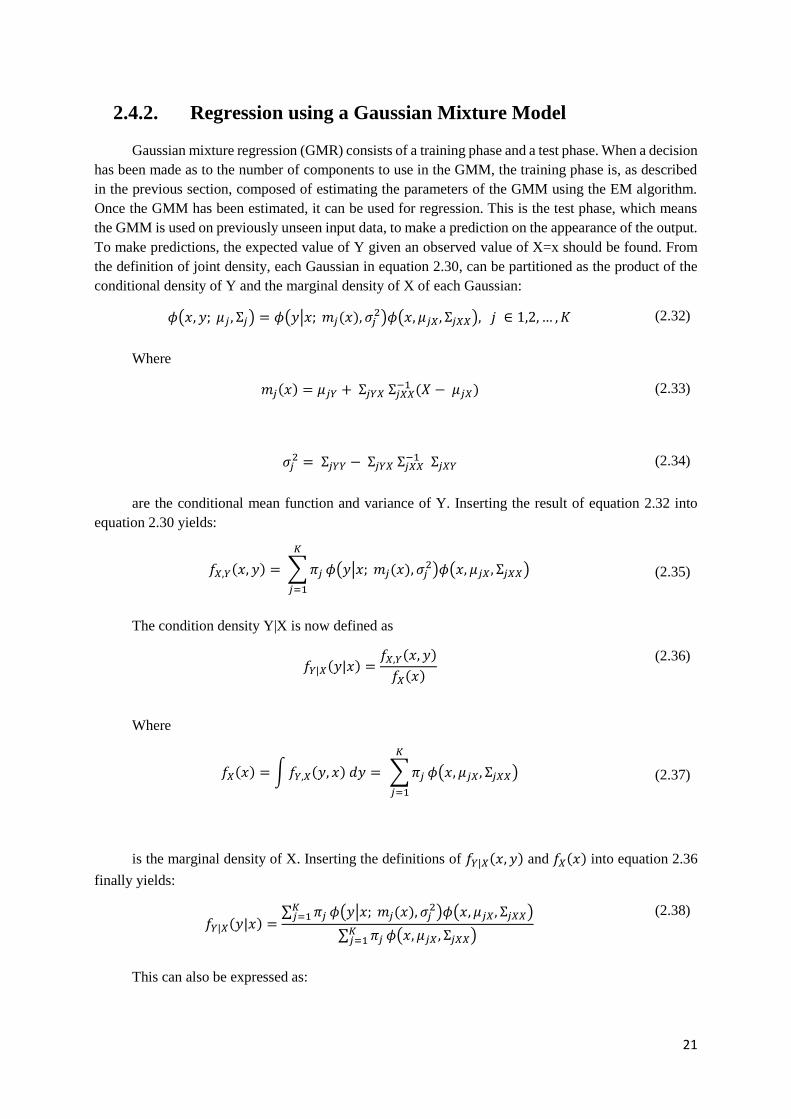
21

2.4.2. Regression using a Gaussian Mixture Model

Gaussian mixture regression (GMR) consists of a training phase and a test phase. When a decision

has been made as to the number of components to use in the GMM, the training phase is, as described

in the previous section, composed of estimating the parameters of the GMM using the EM algorithm.

Once the GMM has been estimated, it can be used for regression. This is the test phase, which means

the GMM is used on previously unseen input data, to make a prediction on the appearance of the output.

To make predictions, the expected value of Y given an observed value of X=x should be found. From

the definition of joint density, each Gaussian in equation 2.30, can be partitioned as the product of the

conditional density of Y and the marginal density of X of each Gaussian:

𝜙(𝑥, 𝑦; 𝜇𝑗 , Σ𝑗) = 𝜙(𝑦|𝑥; 𝑚𝑗(𝑥), 𝜎𝑗2)𝜙(𝑥, 𝜇𝑗𝑋, Σ𝑗𝑋𝑋), 𝑗 ∈ 1,2,… , 𝐾

(2.32)

Where

𝑚𝑗(𝑥) = 𝜇𝑗𝑌 + Σ𝑗𝑌𝑋 Σ𝑗𝑋𝑋−1 (𝑋 − 𝜇𝑗𝑋)

(2.33)

𝜎𝑗2 = Σ𝑗𝑌𝑌 − Σ𝑗𝑌𝑋 Σ𝑗𝑋𝑋

−1 Σ𝑗𝑋𝑌

(2.34)

are the conditional mean function and variance of Y. Inserting the result of equation 2.32 into

equation 2.30 yields:

𝑓𝑋,𝑌(𝑥, 𝑦) = ∑𝜋𝑗

𝐾

𝑗=1

𝜙(𝑦|𝑥; 𝑚𝑗(𝑥), 𝜎𝑗2)𝜙(𝑥, 𝜇𝑗𝑋, Σ𝑗𝑋𝑋)

(2.35)

The condition density Y|X is now defined as

𝑓𝑌|𝑋(𝑦|𝑥) =

𝑓𝑋,𝑌(𝑥, 𝑦)

𝑓𝑋(𝑥)

(2.36)

Where

𝑓𝑋(𝑥) = ∫𝑓𝑌,𝑋(𝑦, 𝑥) 𝑑𝑦 = ∑𝜋𝑗

𝐾

𝑗=1

𝜙(𝑥, 𝜇𝑗𝑋, Σ𝑗𝑋𝑋)

(2.37)

is the marginal density of X. Inserting the definitions of 𝑓𝑌|𝑋(𝑥, 𝑦) and 𝑓𝑋(𝑥) into equation 2.36

finally yields:

𝑓𝑌|𝑋(𝑦|𝑥) =

∑ 𝜋𝑗𝐾𝑗=1 𝜙(𝑦|𝑥; 𝑚𝑗(𝑥), 𝜎𝑗

2)𝜙(𝑥, 𝜇𝑗𝑋, Σ𝑗𝑋𝑋)

∑ 𝜋𝑗𝐾𝑗=1 𝜙(𝑥, 𝜇𝑗𝑋 , Σ𝑗𝑋𝑋)

(2.38)

This can also be expressed as:

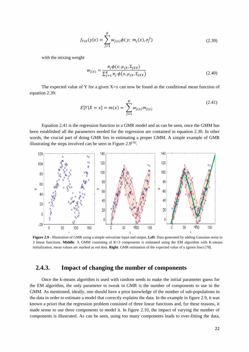
22

𝑓𝑌|𝑋(𝑦|𝑥) =∑𝑤𝑗(𝑥)𝜙(

𝐾

𝑗=1

𝑦; 𝑚𝑗(𝑥), 𝜎𝑗2)

(2.39)

with the mixing weight

𝑤𝑗(𝑥) =

𝜋𝑗𝜙(𝑥; 𝜇𝑗𝑋 , Σ𝑗𝑋𝑋)

∑ 𝜋𝑗𝐾𝑗=1 𝜙(𝑥, 𝜇𝑗𝑋, Σ𝑗𝑋𝑋)

(2.40)

The expected value of Y for a given X=x can now be found as the conditional mean function of

equation 2.39:

𝐸[𝑌|𝑋 = 𝑥] = 𝑚(𝑥) = ∑𝑤𝑗(𝑥)𝑚𝑗(𝑥)

𝐾

𝑗=1

(2.41)

Equation 2.41 is the regression function in a GMR model and as can be seen, once the GMM has

been established all the parameters needed for the regression are contained in equation 2.30. In other

words, the crucial part of doing GMR lies in estimating a proper GMM. A simple example of GMR

illustrating the steps involved can be seen in Figure 2.9[78].

2.4.3. Impact of changing the number of components

Once the k-means algorithm is used with random seeds to make the initial parameter guess for

the EM algorithm, the only parameter to tweak in GMR is the number of components to use in the

GMM. As mentioned, ideally, one should have a prior knowledge of the number of sub-populations in

the data in order to estimate a model that correctly explains the data. In the example in figure 2.9, it was

known a priori that the regression problem consisted of three linear functions and, for these reasons, it

made sense to use three components to model it. In figure 2.10, the impact of varying the number of

components is illustrated. As can be seen, using too many components leads to over-fitting the data,

Figure 2.9 - Illustration of GMR using a simple univariate input and output. Left: Data generated by adding Gaussian noise to

3 linear functions. Middle: A GMM consisting of K=3 components is estimated using the EM algorithm with K-means

initialization, mean values are marked as red dots. Right: GMR estimation of the expected value of y (green line) [78].

23

which is undesirable if noise is present. Also, over-fitting also leads to a more complex model, making

more difficult the correct estimation of the model and the comprehension of it. On the other hand, using

too few components leads to a higher degree of smoothing of the data, which may mean that important

variations are missed. This is called under-fitting. Thus, the goal is to choose a model that is simple as

possible by choosing the smallest number of components that can explain all the important variations in

the data. However, with real-world multidimensional data, it can be difficult to know how many

components should be used. A way to find the optimal number of components is to set up a measure of

regression accuracy, evaluate different models and choose the one that performs best[78].

The Akaike information criterion (AIC) is a measure of the relative quality of statistical models

for a given set of data[79]. Given a collection of models for the data, AIC estimates the quality of each

model, relative to each of the other models. Thus, AIC can be calculated using

𝐴𝐼𝐶 = 2𝑘 − 2 ln(�̂�)

(2.42)

Where k is the number of components in GMM and �̂� = 𝑝(𝑋, 𝑌|𝜃), designed by likelihood. Given

a set of candidate models for the data, the preferred model is the one with the minimum AIC value. AIC

rewards goodness of fit (as assessed by the likelihood function), but it also includes a penalty that is an

increasing function of the number of estimated parameters. The penalty discourages over-fitting,

because increasing the number of parameters in the model almost always improves the goodness of fit.

In this way, the simplest model as possible that can explain the data can be determined.

Figure 2.10 – Illustration of GMR using different number of components. Data is the same as in figure 2.9. Left: The GMM

has been estimated using 25 components (over-fitting). Right: The GMM has been estimated using 2 components (under-

fitting) [78].

24

Chapter 3

Methods and Materials

3.1. Data Specification

This study includes data from 6 anonymized prostate cancer patients (Patients 1 to 6). The datasets

for each patient include a 3D CT image and a 3D MRI dataset, which were not acquired on the same

day. Small discrepancies o the anatomy of the patient may be observed due to inter-scan variation caused

by repositioning and the non-simultaneity of the acquisitions.

3.1.1. CT acquisition

Pelvic CT images were acquired using a Brilliance Big Bore (Philips Medical Systems, Best, The

Netherlands) scanner operated at 120 KVp, with a 512 x 512 in-plane reconstruction. For patient 1, 1.28

x 1.28 mm2 in-plane image dimensions with a slice thickness of 5 mm were used. For the remaining

patients, 0.84 x 0.84 mm2 in-plane image dimensions with a slice thickness of 5 mm were used. Specific

immobilization devices, such as a knee wedge and a flat table top, were used during imaging.

3.1.2. MR acquisition

Pelvic MR images were acquired using an Ingenia 3.0 T system (Philips Medical Systems, Best,

The Netherlands. A T1-weighted Fast Field Echo sequence was acquired for all the patients using three

echoes (TE=2.1/3.5/4.9 ms, TR=6.8 ms, Flip angle= 10°, Bandwidth=1122 Hz/pixel). The images were

reconstructed with 336 x 336 x 75 matrix dimensions with an isotropic voxel size of 1.2 x 1.2 x 1.2 mm3.

3.2. MR/CT Registration

The MR/CT image registration was done using the Elastix Registration software (Image Science

Institute, Utrecht, The Netherlands)[80]. The MR data was considered as reference due to its smaller slice

thickness. The process of registration was accomplished using two transformations, both using a mutual

information algorithm.

First, in order to obtain a first alignment between the MR and CT data, the CT image was first

registered using a rigid transformation[81]. However, due to inter-scan variation, some differences in

patient’s anatomy that could not be solved by a rigid registration were found.

Thus, a non-rigid registration was applied using a cubic bspline transformation[82]. However, bone

anatomy is rigid and, therefore, a non-rigid registration cannot be applied to it, as it may cause unreal

deformations. By applying a rigidity penalty, this problem may be solved[83]. The rigidity penalty defines

areas where the registration should be governed by a rigid transformation by including a binary mask of

these areas as an input to the registration process. Thus, a bone binary mask was derived, using the

following procedure, as illustrated in figure 3.1:

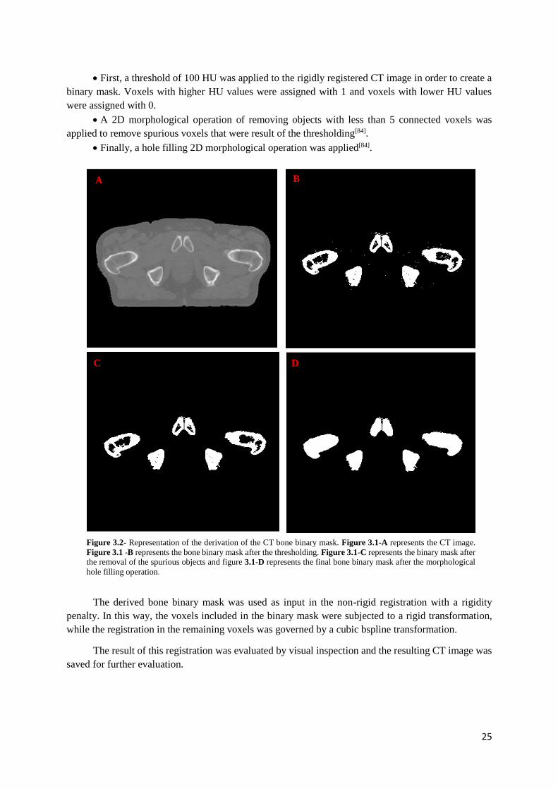
25

• First, a threshold of 100 HU was applied to the rigidly registered CT image in order to create a

binary mask. Voxels with higher HU values were assigned with 1 and voxels with lower HU values

were assigned with 0.

• A 2D morphological operation of removing objects with less than 5 connected voxels was

applied to remove spurious voxels that were result of the thresholding[84].

• Finally, a hole filling 2D morphological operation was applied[84].

The derived bone binary mask was used as input in the non-rigid registration with a rigidity

penalty. In this way, the voxels included in the binary mask were subjected to a rigid transformation,

while the registration in the remaining voxels was governed by a cubic bspline transformation.

The result of this registration was evaluated by visual inspection and the resulting CT image was

saved for further evaluation.

Figure 3.2- Representation of the derivation of the CT bone binary mask. Figure 3.1-A represents the CT image.

Figure 3.1 -B represents the bone binary mask after the thresholding. Figure 3.1-C represents the binary mask after

the removal of the spurious objects and figure 3.1-D represents the final bone binary mask after the morphological

hole filling operation.

A B

C D

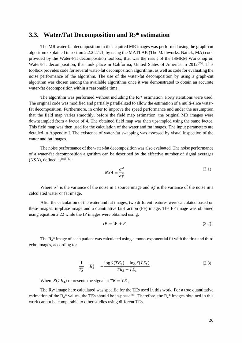
26

3.3. Water/Fat Decomposition and R2* estimation

The MR water-fat decomposition in the acquired MR images was performed using the graph-cut

algorithm explained in section 2.2.2.2.1.1, by using the MATLAB (The Mathworks, Natick, MA) code

provided by the Water-Fat decomposition toolbox, that was the result of the ISMRM Workshop on

Water/Fat decomposition, that took place in California, United States of America in 2012[85]. This

toolbox provides code for several water-fat decomposition algorithms, as well as code for evaluating the

noise performance of the algorithm. The use of the water-fat decomposition by using a graph-cut

algorithm was chosen among the available algorithms once it was demonstrated to obtain an accurate

water-fat decomposition within a reasonable time.

The algorithm was performed without including the R2* estimation. Forty iterations were used.

The original code was modified and partially parallelized to allow the estimation of a multi-slice water-

fat decomposition. Furthermore, in order to improve the speed performance and under the assumption

that the field map varies smoothly, before the field map estimation, the original MR images were

downsampled from a factor of 4. The obtained field map was then upsampled using the same factor.

This field map was then used for the calculation of the water and fat images. The input parameters are

detailed in Appendix I. The existence of water-fat swapping was assessed by visual inspection of the

water and fat images.

The noise performance of the water-fat decomposition was also evaluated. The noise performance

of a water-fat decomposition algorithm can be described by the effective number of signal averages

(NSA), defined as[86] [87]:

𝑁𝑆𝐴 =

𝜎2

𝜎𝑃2

(3.1)

Where 𝜎2 is the variance of the noise in a source image and 𝜎𝑃2 is the variance of the noise in a

calculated water or fat image.

After the calculation of the water and fat images, two different features were calculated based on

these images: in-phase image and a quantitative fat-fraction (FF) image. The FF image was obtained

using equation 2.22 while the IP images were obtained using:

𝐼𝑃 = 𝑊 + 𝐹 (3.2)

The R2* image of each patient was calculated using a mono-exponential fit with the first and third

echo images, according to:

1

𝑇2∗ = 𝑅2

∗ = −log 𝑆(𝑇𝐸3) − log 𝑆(𝑇𝐸1)

𝑇𝐸3 − 𝑇𝐸1

(3.3)

Where 𝑆(𝑇𝐸3) represents the signal at 𝑇𝐸 = 𝑇𝐸3.

The R2* image here calculated was specific for the TEs used in this work. For a true quantitative

estimation of the R2* values, the TEs should be in-phase[88]. Therefore, the R2* images obtained in this

work cannot be comparable to other studies using different TEs.

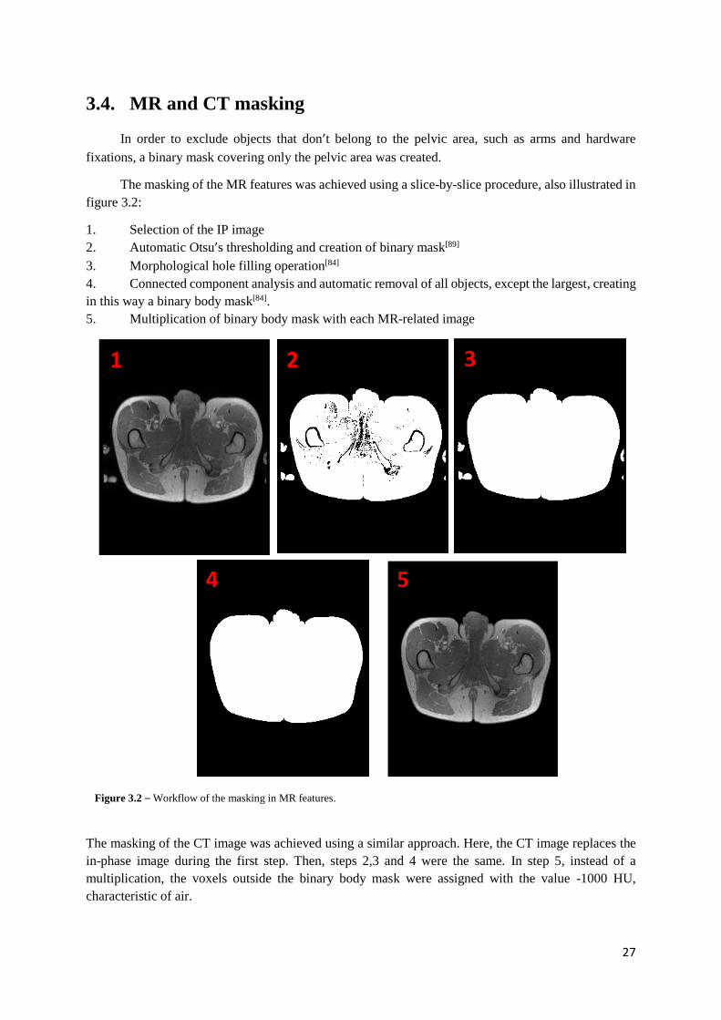
27

3.4. MR and CT masking

In order to exclude objects that don’t belong to the pelvic area, such as arms and hardware

fixations, a binary mask covering only the pelvic area was created.

The masking of the MR features was achieved using a slice-by-slice procedure, also illustrated in

figure 3.2:

1. Selection of the IP image

2. Automatic Otsu’s thresholding and creation of binary mask[89]

3. Morphological hole filling operation[84]

4. Connected component analysis and automatic removal of all objects, except the largest, creating

in this way a binary body mask[84].

5. Multiplication of binary body mask with each MR-related image

The masking of the CT image was achieved using a similar approach. Here, the CT image replaces the

in-phase image during the first step. Then, steps 2,3 and 4 were the same. In step 5, instead of a

multiplication, the voxels outside the binary body mask were assigned with the value -1000 HU,

characteristic of air.

1 2 3

4 5

Figure 3.2 – Workflow of the masking in MR features.

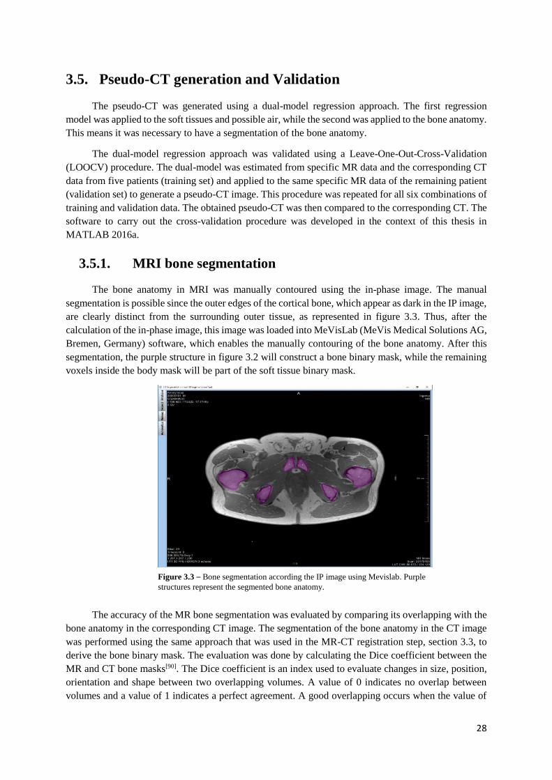
28

3.5. Pseudo-CT generation and Validation

The pseudo-CT was generated using a dual-model regression approach. The first regression

model was applied to the soft tissues and possible air, while the second was applied to the bone anatomy.

This means it was necessary to have a segmentation of the bone anatomy.

The dual-model regression approach was validated using a Leave-One-Out-Cross-Validation

(LOOCV) procedure. The dual-model was estimated from specific MR data and the corresponding CT

data from five patients (training set) and applied to the same specific MR data of the remaining patient

(validation set) to generate a pseudo-CT image. This procedure was repeated for all six combinations of

training and validation data. The obtained pseudo-CT was then compared to the corresponding CT. The

software to carry out the cross-validation procedure was developed in the context of this thesis in

MATLAB 2016a.

3.5.1. MRI bone segmentation

The bone anatomy in MRI was manually contoured using the in-phase image. The manual

segmentation is possible since the outer edges of the cortical bone, which appear as dark in the IP image,

are clearly distinct from the surrounding outer tissue, as represented in figure 3.3. Thus, after the

calculation of the in-phase image, this image was loaded into MeVisLab (MeVis Medical Solutions AG,

Bremen, Germany) software, which enables the manually contouring of the bone anatomy. After this

segmentation, the purple structure in figure 3.2 will construct a bone binary mask, while the remaining

voxels inside the body mask will be part of the soft tissue binary mask.

The accuracy of the MR bone segmentation was evaluated by comparing its overlapping with the

bone anatomy in the corresponding CT image. The segmentation of the bone anatomy in the CT image

was performed using the same approach that was used in the MR-CT registration step, section 3.3, to

derive the bone binary mask. The evaluation was done by calculating the Dice coefficient between the

MR and CT bone masks[90]. The Dice coefficient is an index used to evaluate changes in size, position,

orientation and shape between two overlapping volumes. A value of 0 indicates no overlap between

volumes and a value of 1 indicates a perfect agreement. A good overlapping occurs when the value of

Figure 3.3 – Bone segmentation according the IP image using Mevislab. Purple

structures represent the segmented bone anatomy.

29

the Dice coefficient is higher than 0.7[91]. In the context of this work, the Dice coefficient was calculated

as following:

𝐷𝑖𝑐𝑒 𝑐𝑜𝑒𝑓𝑓𝑖𝑐𝑖𝑒𝑛𝑡 =

2(𝐵𝑜𝑛𝑒𝐶𝑇 ∩ 𝐵𝑜𝑛𝑒𝑀𝑅)

𝐵𝑜𝑛𝑒𝐶𝑇 ∪ 𝐵𝑜𝑛𝑒𝑀𝑅

(3.4)

Where 𝐵𝑜𝑛𝑒𝐶𝑇 represents the bone mask in the CT image and 𝐵𝑜𝑛𝑒𝑀𝑅 the bone mask that was

manually segmented.

3.5.2. Soft tissue HU conversion model

The possibility to construct a pelvic soft tissue HU conversion model was investigated by

comparing the quantitative FF values in soft tissue with the corresponding HU values in the CT image.

As soft tissues are mainly constituted by water (muscle) or fat, a relative measure of the amount of water

and fat signal within a voxel was considered sufficient. Possible existing air was also included in this

model. The relation between FF values in soft tissue and HU values was obtained through a polynomial

fit:

𝐻𝑈 = 𝑎 + 𝑏×𝐹𝐹 + 𝑐×𝐹𝐹2 + …

(3.5)

Where 𝑎, 𝑏, 𝑐 are the fitting parameters of the polynomial model and FF is the fat fraction in a

voxel.

The order for the polynomial fit was chosen based on the minimization of the mean absolute error

(MAE) between the obtained pseudo-CT and the real CT. Further description of MAE is provided in

section 3.6.4. Thus, the LOOCV procedure was carried out for soft tissue areas using different

polynomial orders. Then, the polynomial order that leads to a lower MAE was chosen to be used in the

pseudo-CT generation procedure, and the results were saved for future application.

3.5.3. HU conversion model for bone anatomy

A MATLAB implementation of Gaussian mixture regression was used throughout this project[92].

This implementation used the built-in k-means function of the MATLAB Statistics toolbox to give an

initial estimate of the component mean values and covariance matrices for the EM algorithm. EM was

stopped when the increase in the log-likelihood value was smaller than 10-10. The input variables (X)

were MR related features while the output (Y) is the CT image. This toolbox was used instead of the

MATLAB built-in functions due to its superior speed performance.

The R2*, fat, water and fat fraction images that were previously calculated were included in the

bone regression model. The inclusion of this set of variables as an intuitive explanation. The R2* image

provides information about the T2* decay, which was proven to be correlated with the bone mineral

density[17][24] [25] [26] [27]. Moreover, the FF image provides information about the relative presence of fat

or water within a voxel and it was also proven to be correlated with the bone mineral density. At last,

the water and fat images provide information about the signal intensity of these species when they are

in-phase. As the MR sequence used in this project was a gradient-echo sequence type and the signal

intensity is governed by the T2* decay, the water and fat images can also provide information about it,

at the same time that they provide information about the source of the signal.

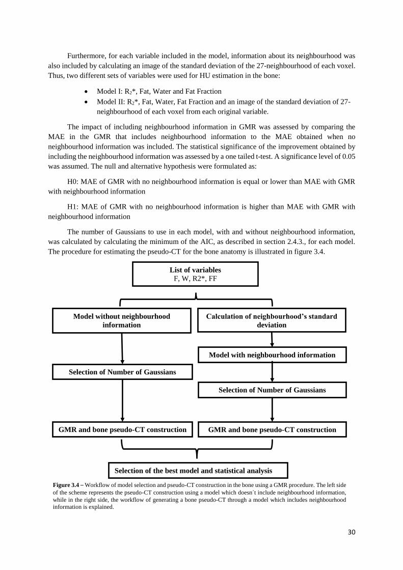
30

Furthermore, for each variable included in the model, information about its neighbourhood was

also included by calculating an image of the standard deviation of the 27-neighbourhood of each voxel.

Thus, two different sets of variables were used for HU estimation in the bone:

• Model I: R2*, Fat, Water and Fat Fraction

• Model II: R2*, Fat, Water, Fat Fraction and an image of the standard deviation of 27-

neighbourhood of each voxel from each original variable.

The impact of including neighbourhood information in GMR was assessed by comparing the

MAE in the GMR that includes neighbourhood information to the MAE obtained when no

neighbourhood information was included. The statistical significance of the improvement obtained by

including the neighbourhood information was assessed by a one tailed t-test. A significance level of 0.05

was assumed. The null and alternative hypothesis were formulated as:

H0: MAE of GMR with no neighbourhood information is equal or lower than MAE with GMR

with neighbourhood information

H1: MAE of GMR with no neighbourhood information is higher than MAE with GMR with

neighbourhood information

The number of Gaussians to use in each model, with and without neighbourhood information,

was calculated by calculating the minimum of the AIC, as described in section 2.4.3., for each model.

The procedure for estimating the pseudo-CT for the bone anatomy is illustrated in figure 3.4.

List of variables F, W, R2*, FF

Model with neighbourhood information

Calculation of neighbourhood’s standard

deviation

GMR and bone pseudo-CT construction

Selection of the best model and statistical analysis

Model without neighbourhood

information

Selection of Number of Gaussians

GMR and bone pseudo-CT construction

Selection of Number of Gaussians

Figure 3.4 – Workflow of model selection and pseudo-CT construction in the bone using a GMR procedure. The left side

of the scheme represents the pseudo-CT construction using a model which doesn´t include neighbourhood information,

while in the right side, the workflow of generating a bone pseudo-CT through a model which includes neighbourhood

information is explained.

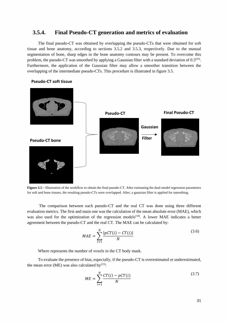
31

3.5.4. Final Pseudo-CT generation and metrics of evaluation

The final pseudo-CT was obtained by overlapping the pseudo-CTs that were obtained for soft

tissue and bone anatomy, according to sections 3.5.2 and 3.5.3, respectively. Due to the manual

segmentation of bone, sharp edges in the bone anatomy contours may be present. To overcome this

problem, the pseudo-CT was smoothed by applying a Gaussian filter with a standard deviation of 0.5[93].

Furthermore, the application of the Gaussian filter may allow a smoother transition between the

overlapping of the intermediate pseudo-CTs. This procedure is illustrated in figure 3.5.

The comparison between each pseudo-CT and the real CT was done using three different

evaluation metrics. The first and main one was the calculation of the mean absolute error (MAE), which

was also used for the optimization of the regression models[18]. A lower MAE indicates a better

agreement between the pseudo-CT and the real CT. The MAE can be calculated by:

𝑀𝐴𝐸 =∑|𝑝𝐶𝑇(𝑖) − 𝐶𝑇(𝑖)|

𝑁

𝑁

𝑖=1

(3.6)

Where represents the number of voxels in the CT body mask.

To evaluate the presence of bias, especially, if the pseudo-CT is overestimated or underestimated,

the mean error (ME) was also calculated by[23]:

𝑀𝐸 =∑𝐶𝑇(𝑖) − 𝑝𝐶𝑇(𝑖)

𝑁

𝑁

𝑖=1

(3.7)

Final Pseudo-CT

Gaussian Filter

Pseudo-CT soft tissue

Pseudo-CT bone

Pseudo-CT

Figure 3.5 – Illustration of the workflow to obtain the final pseudo-CT. After estimating the dual-model regression parameters

for soft and bone tissues, the resulting pseudo-CTs were overlapped. After, a gaussian filter is applied for smoothing.

32

Furthermore, the peak signal.to-noise-ratio, PSNR, was also computed. This metric calculates the

ratio between the maximum possible power of a signal or image and the power of corrupting noise that

affects the fidelity of its representation. A higher value of PSNR represents a better reconstruction.

PSNR is usually expressed in terms of the logarithmic decibel (dB) scale and it can be calculated by:

𝑃𝑆𝑁𝑅 = 10 log10 (

𝑀𝐴𝑋2(𝐶𝑇)

𝑀𝑆𝐸)

(3.8)

Where 𝑀𝐴𝑋(𝐶𝑇) represents the maximum HU value in CT image and MSE the mean squared

error:

𝑀𝑆𝐸 =∑(𝐶𝑇(𝑖) − 𝑝𝐶𝑇(𝑖)

𝑁)

2𝑁

𝑖=1

(3.9)

Furthermore, the structural similarity (SSIM) index was also used for measuring the similarity

between the pseudo-CT and the real CT. This metric, in contrast to the other methods, also incorporates

perceptual phenomena, including both luminance and contrast in the calculation. Higher values of SSIM

demonstrate a better agreement between the two images. SSIM can be calculated using:

𝑆𝑆𝐼𝑀(𝑝𝐶𝑇, 𝐶𝑇) =

(2𝜇𝑝𝐶𝑇𝜇𝐶𝑇 + 𝐶1)(2𝜎𝑝𝐶𝑇,𝐶𝑇 + 𝐶2)

(𝜇𝑝𝐶𝑇2 + 𝜇𝐶𝑇

2 + 𝐶1)(𝜎𝑝𝐶𝑇2 + 𝜎𝐶𝑇

2 + 𝐶2)

(3.10)

Where 𝜇𝑝𝐶𝑇 , 𝜇𝐶𝑇 and 𝜎𝑝𝐶𝑇2 , 𝜎𝐶𝑇

2 are the average and variance values of the pseudo-CT and CT,

respectively, 𝜎𝑝𝐶𝑇,𝐶𝑇 is the covariance between the pseudo-CT and the CT. 𝐶1 = (𝑘1𝐿)2 and 𝐶2 =

(𝑘2𝐿)2 are two variables to stabilize the division, where 𝐿 is the dynamic range of the pixel-values. By

default, 𝑘1 = 0.01 and 𝑘2 = 0.03.

33

Chapter 4

Results and Discussion

4.1. Water-Fat Decomposition and R2* estimation

Figure 4.1 shows the obtained maps by performing the water-fat decomposition without R2* estimation.

Figure 4.1-A and 4.1-B represent the fat and water-only images, respectively. As it can be seen in these

figures, an accurate separation of the water and fat signal was achieved. Also, no water-fat swapping

was found by visual inspection. Although no water-fat swaps were seen, some leakage of the fat signal

into the water image was observed, as represented by the green arrow in figure 4.1-B. This leakage of

the fat signal can be explained by the bipolar readout gradient that was used in this study to increase the

scan efficiency and to allow the use of a shorter echo spacing, in order to eventually decrease the

scanning time. When using bipolar readout gradients, the field map may comprise significant

contributions from eddy currents caused by the bipolar readout gradient, that alternate with the readout

gradient and thus violate the linear relation between the field map and TE assumed by a 3-echo method.

An eddy-current correction method may be applied to correct for the presence of eddy-currents, but it

was beyond the scope of this project[54]. Figure 4.1-C represents the field map obtained. As, a smooth

field map was obtained, excepting for some tissue-air interfaces. The presence of air complicates the

estimation of the field map. However, it did not result in water-fat swaps.

The noise performance of this algorithm was also studied, by calculating the NSA map for the fat and

water images, as illustrated in figure 4.2-A and 4.2-B, respectively. Theoretically, for a water-fat

B A C

Figure 4.1 – Illustration of the results obtained through the water-fat decomposition algorithm without R2* estimation. Figure

4.1-A represents the fat image, figure 4.1-B the water image with the green arrow representing the effect of eddy currents

and figure 4.1-C illustrates the obtained field map in Hertz. All these images are from patient 2.

34

algorithm that uses 3 echoes, the maximum value of NSA that can be obtained is 3, since only 3 echoes

are used. As it can be seen in those figures, most voxels have values higher than 2 and close to 3. For

the 6 patients used in this study, an average NSA of 2.64 ± 0.03 was achieved for the water images.

Regarding the fat images, the average NSA was 2.66 ± 0.05 for the 6 patients. These values prove that

the use of a graph-cut algorithm for water-fat decomposition without R2* estimation has a noise

performance close to the optimal values when only 3 echoes are used, proving the high SNR

performance of this algorithm.

Then, the R2* map was calculated, as it can be seen in figure 4.3. This R2* map is specific for the

TEs used in this project. Normally, an R2* value is specific for each tissue, regarding all the acquisition

parameters, if the calculation is performed when the water and fat signal are in-phase. If this happens,

the R2* map can be used for the assessment of iron concentration among other applications[26]. The TEs

of the first and third echo used in this study are not completely in-phase, causing the R2* values to

depend on the actual TE values. However, as it can be seen in figure 4.3, this “apparent” R2* map is

capable of providing contrast between the different tissue types. This is clearly visible from the figure

4.3, showing that water, fat and bone tissues present different R2* values.

A B

Figure 4.2- Illustration of NSA maps obtained for patient 2 when the water-fat decomposition algorithm is performed without

R2* estimation. Figure 4.2-A represents the NSA map of the fat image, while figure 4.2-B represents the NSA map of the

water image.

Figure 4.3 – Illustration of R2* map of patient 2. The R2* values are

described in terms of ms-1

35

A possible solution to estimate a “true” R2* image relies on estimating it jointly with the water

and fat images, by including it in the decomposition algorithm. As already referred, the water-fat

decomposition algorithm allows the R2* estimation. Theoretically, the simultaneous water-fat

decomposition and R2* estimation may be performed using three echoes. However, in the presence of

noise, the algorithm may become very unstable when only three images are acquired. Figure 4.4

illustrates the results obtained by using the water-fat decomposition algorithm that includes the R2*

estimation. It is possible to observe that the water and fat images, figures 4.4-A and 4.4-B respectively,

present a noisier decomposition, especially the water image. In this image, we can see that the left part

of the body presents more troubles, since the issues related to the leakage of the fat signal are even more

visible. Also, the R2* estimation is not accurate, since there are discrepancies in the estimated R2* values

for a single tissue type. It is well known that a single tissue type should have a homogeneous R2* value.

As it can be seen in figure 4.4-C, the R2* values are different for the same tissue type, varying from the

left part of the body to the right part. This discrepancy is especially visible in muscle, where in the left

part of the body, the R2* values are clearly distinguishable from the surrounding tissues, while in the

right part, there is no contrast between the R2* value of muscle and the R2* values of the surrounding

fat. It is also important to notice that, while in the water image it is the left part of the body that is more

affected by the presence of noise, in the R2* map it is the right part of body that presents these difficulties.

The fact that the water-fat decomposition with R2* estimation is noisier than the one performed without

R2* estimation is most likely caused by its high sensitivity to noise when only 3 echoes are collected.

As referred before, each echo contributes with an imaginary and a real image. Thus, the number of input

images to include in the water-fat decomposition algorithm is 6. If the R2* estimation is included in the

procedure, the number of unknows to estimate is 6 (real and imaginary fat, real and imaginary water,

field map and R2* map), while without R2* estimation the number of unknows is only 5. Although

theoretically, to obtain an accurate water-fat decomposition as well as the R2* map, the number of input

images has to be equal or higher than the number of unknows, this may not hold when noise is present.

Thus, using 6 input images to obtain 6 unknowns may turn the algorithm very sensitive to noise. When

only 5 unknowns are estimated, the remaining input image may be used for noise compensation. In this

way, it can be concluded that for performing the R2* estimation, the number of input images used in the

algorithm has to be always higher than the number of unknowns to be estimated. Acquiring one more

echo, it would be possible to estimate the R2* map without having problems related to noise

performance. However, this would increase the scanning time. In figure 4.4-D, we can see the obtained

field map. This field map is similar to the field map obtained when no R2* estimation is made. Since the

field map estimation is the first step of the water-fat decomposition algorithm, it is less influenced by

noise.

36

The influence of noise in water-fat decomposition including the R2* estimation was also evaluated

by calculating the NSA maps of the water and fat images in order to evaluate the noise performance.

Figures 4.5-A and 4.5-B illustrate these NSA maps of the fat and water images, respectively. It is visible

that the NSA values for both images are significantly lower than the optimal value of 3 for 3-echoes

water-fat decomposition algorithms[87]. An average NSA value of 1.18±0.07 for the NSA map of the fat

image, while the average NSA value of the water image was 0.67±0.10. By comparing these NSA values

with the ones obtained using the water-fat decomposition algorithm without R2* estimation, it is possible

to conclude that the inclusion of the R2* estimation leads to a poorer noise performance when only

3echoes are included, as well as an inaccurate R2* map.

B

D C

A

Figure 4.4 - Illustration of the results obtained through the water-fat decomposition algorithm with R2* estimation. Figure

4.4-A represents the fat image, figure 4.4-B the water image. Figure 4-C illustrates the obtained R2* map, while figure

4-D represents the obtained field map (Hertz). All these images are from patient 2.

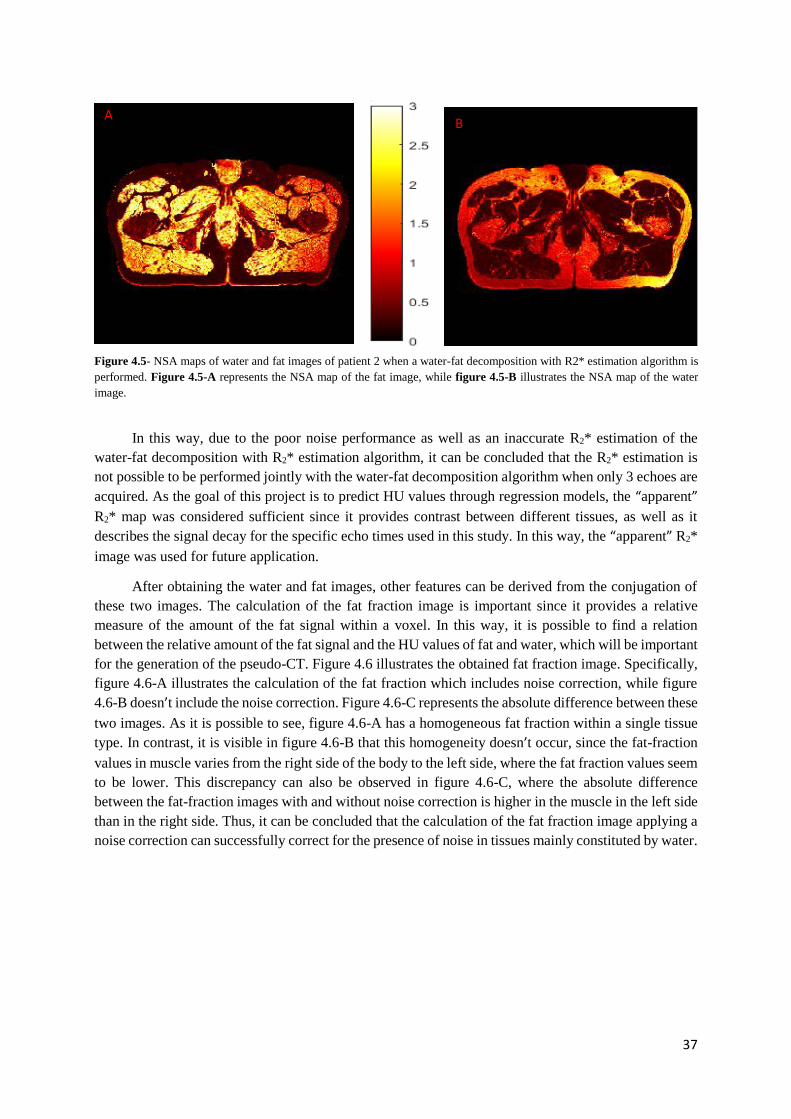
37

In this way, due to the poor noise performance as well as an inaccurate R2* estimation of the

water-fat decomposition with R2* estimation algorithm, it can be concluded that the R2* estimation is

not possible to be performed jointly with the water-fat decomposition algorithm when only 3 echoes are

acquired. As the goal of this project is to predict HU values through regression models, the “apparent”

R2* map was considered sufficient since it provides contrast between different tissues, as well as it

describes the signal decay for the specific echo times used in this study. In this way, the “apparent” R2*

image was used for future application.

After obtaining the water and fat images, other features can be derived from the conjugation of

these two images. The calculation of the fat fraction image is important since it provides a relative

measure of the amount of the fat signal within a voxel. In this way, it is possible to find a relation

between the relative amount of the fat signal and the HU values of fat and water, which will be important

for the generation of the pseudo-CT. Figure 4.6 illustrates the obtained fat fraction image. Specifically,

figure 4.6-A illustrates the calculation of the fat fraction which includes noise correction, while figure

4.6-B doesn’t include the noise correction. Figure 4.6-C represents the absolute difference between these

two images. As it is possible to see, figure 4.6-A has a homogeneous fat fraction within a single tissue

type. In contrast, it is visible in figure 4.6-B that this homogeneity doesn’t occur, since the fat-fraction

values in muscle varies from the right side of the body to the left side, where the fat fraction values seem

to be lower. This discrepancy can also be observed in figure 4.6-C, where the absolute difference

between the fat-fraction images with and without noise correction is higher in the muscle in the left side

than in the right side. Thus, it can be concluded that the calculation of the fat fraction image applying a

noise correction can successfully correct for the presence of noise in tissues mainly constituted by water.

A B

Figure 4.5- NSA maps of water and fat images of patient 2 when a water-fat decomposition with R2* estimation algorithm is

performed. Figure 4.5-A represents the NSA map of the fat image, while figure 4.5-B illustrates the NSA map of the water

image.

38

Furthermore, also the in-phase image was calculated based on the water and fat images. The in-

phase image allows the distinction between low-signal and high-signal areas, as it can be seen in figure

4.7-A. In this figure, it is possible to see that the cortical bone appears as dark due to its fast T2* decay.

This facilitates the manual segmentation of the bone, since there is a contrast between the outer edge of

the cortical bone and the surrounding tissue, as it can be seen from the figure 4.7-B. In this figure, the

signal profile along a line that crosses a bone structure (green line in figure 4.7-A) is represented,

allowing to see the contrast between the outer edges of the bone structures and the surrounding tissue.

Outer

edge

of

bone

Outer

edge of

bone

Figure 4.7 – Representation of in-phase mage obtained for patient 2 in Figure 4.7-A. The green line represents a row

where the signal profile is represented in Figure 4.7-B. As it can be seen the outer edges of the bone structure crossed by

the green line are clearly distinguishable from the surrounding tissue, allowing the bone segmentation.

A B

A B C

Figure 4.6 – Illustration of the fat fraction images obtained for patient 2. Figure 4.6-A represents the fat fraction obtained

using a noise correction approach, while figure 4.6-B doesn’t include the correction of the noise. Figure 4.6-C illustrates the

absolute difference between figure 4.6-A and 4.7-B.

39

The estimation of the water-fat decomposition related images, as well as the R2* image was

performed using an Intel 7 Core computer, with 2.6 GHz and 16 Gb of RAM, and for each patient, it

had the duration of 217 seconds.

4.2. Pseudo-CT generation

4.2.1. MRI bone segmentation

The accuracy of the manual bone segmentation that was performed using the in-phase image was

evaluated by calculating the Dice Score, having as reference the previously segmented bone anatomy in

the CT image.

Figure 4.8 illustrates the obtained Dice Score per patient. An average Dice Score of 0.91±0.02

was obtained for all the patients, showing a good agreement between the bone segmentation in CT and

MRI. The errors that were obtained may be explained by the natural ambiguity that the manual

segmentation has, leading to imperfections when contouring the bone anatomy. Also, registrations errors

are an important source of error, since a perfect alignment between the CT image and the MRI is almost

impossible to obtain. Furthermore, the quality of the registration was assessed by visual inspection,

leading to errors related to the subjectivity of the human condition. These contouring and registration

errors will not be only important in the evaluation of the bone segmentation, but also in the subsequent

steps of the pseudo-CT, since the errors are propagated throughout the whole pseudo-CT generation

procedure.

4.2.2. Soft tissue HU conversion model

As soft tissues are mainly constituted by water (muscle) and/or fat, a quantitative measure of the

MR signal present in a voxel may be useful to estimate the HU values in soft tissues. As the fat fraction

provides the relative amount of fat signal in a voxel, it may be used for HU estimation.

Figure 4.8 – Bone dice score per patient between the bone MR segmentation and the CT

bone tissues

40

Thus, Figure 4.9 represents the joint histogram of the fat fraction and the HU units in the soft

tissue mask. As it can be seen, most of the tissues with a lower fat fraction (FF<50%), representing

tissues mostly constituted by water, have a HU between 0 and 100, which is the typical value for mainly

consisting of water, such as the muscle. Also, fatty tissues (FF>=50%) have HUs between 0 and -100

HU, which again, is the typical values for these tissues in a CT image. Thus, a negative linear correlation

between the HUs and fat fraction values can be found, having a Pearson Correlation Coefficient of -

0.63.

Furthermore, in this joint histogram, it is possible to see the presence of high HU values, typical

of bone, that are related to low fat fractions. The presence of these voxels in the soft tissue mask is due

to the errors in the bone countering which makes that not all the bone tissues in CT are overlapped with

the MR bone mask. Moreover, in the bottom of the joint histogram it is possible to see the presence of

air in the CT images (-1000 HU). This air is located in the rectum. The inclusion of air voxels in the

soft tissue model may be explained for several reasons. First, the urine in the bladder (with HU close to

the water) presents a very long T1 relaxation time, which makes it to appear as dark in T1-weighted

images. In this way, the distinction between the bladder and the air in the rectum becomes difficult.

Also, as the MR and CT images were acquired at different time points and with different patient

positioning, differences in the position and volume of the air in the rectum were observed. These

differences would lead to higher errors when the air MRI and CT air does not overlap consistently. At

last, for dose calculation and attenuation correction purposes, it was proven that the assignment of a soft

tissue HU value to the air in the rectum during pseudo-CT generation didn’t lead to significant errors[70].

However, if a bone HU value was assigned, the error in dose calculations and in attenuation correction

calculations would be significant, proving the necessity of bone segmentation. Thus, it was decided to

include air voxels in the soft tissue conversion model.

The order of the polynomial fit to use in the soft tissue regression model was chosen based on the

minimization of the MAE in soft tissue using the LOOCV procedure. In figure 4.10-A, we can see the

MAE per patient using the first four polynomial orders, while figure 4.10-B illustrates the average MAE

per polynomial order. As it can be seen in these two figures, using the first polynomial leads to a higher

MAE in all patients when compared to the others polynomial orders, which was proven to be statistically

significant (p-value=0.002). In contrast, there was no statistical difference between the means of MAE

Figure 4.9 – Joint histogram between the fat fraction values and the HU values in soft

tissue

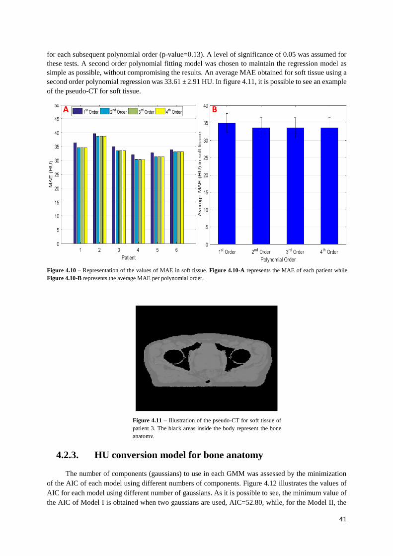
41

for each subsequent polynomial order (p-value=0.13). A level of significance of 0.05 was assumed for

these tests. A second order polynomial fitting model was chosen to maintain the regression model as

simple as possible, without compromising the results. An average MAE obtained for soft tissue using a

second order polynomial regression was 33.61 ± 2.91 HU. In figure 4.11, it is possible to see an example

of the pseudo-CT for soft tissue.

4.2.3. HU conversion model for bone anatomy

The number of components (gaussians) to use in each GMM was assessed by the minimization

of the AIC of each model using different numbers of components. Figure 4.12 illustrates the values of

AIC for each model using different number of gaussians. As it is possible to see, the minimum value of

the AIC of Model I is obtained when two gaussians are used, AIC=52.80, while, for the Model II, the

B A

Figure 4.10 – Representation of the values of MAE in soft tissue. Figure 4.10-A represents the MAE of each patient while

Figure 4.10-B represents the average MAE per polynomial order.

Figure 4.11 – Illustration of the pseudo-CT for soft tissue of

patient 3. The black areas inside the body represent the bone

anatomy.

42

minimum value is obtained when three gaussians are used, AIC=86.70. In this way, Model I, which

doesn’t include neighbourhood information, is modelled by a mixture of two subpopulations. Since, in

contrast to other bone tissues, there is no signal in the cortical bone, the existence of two subpopulations

may be explained. Regarding Model II, which includes neighbourhood information by calculating the

standard deviation of the 27-neighbourhood of each voxel of the MRI features, it is modelled by three

populations. Thus, the inclusion of neighbourhood information may turn the distinction of another

subpopulation of voxels possible. This may be explained by the fact that non-cortical bone tissues may

be divided in bone marrow and cancellous bone, of which the cancellous bone has higher HU values. In

this way, the inclusion of neighbourhood information is capable of modelling these different bone

tissues.

Figure 4.13-A and figure 4.13-B represent the MAE in bone anatomy for each patient and the

average MAE in all the patients, respectively. As it is possible to see, Model II, which includes

neighbourhood information, presents a lower MAE for every patient as well as a lower average MAE

than Model I, which doesn’t include the neighbourhood information. The average MAE of Model II was

101.49±10.80 HU, while the MAE obtained for Model I was 113.99±17.72 HU. Thus, it is possible to

conclude that the inclusion of neighbourhood information in GMR leads to a significantly lower MAE,

p-value=0.02, using a significance level of 0.05. However, the superior predicting performance of the

the model including neighbourhood information may be related to the fact that more Gaussian

components are used in the parameter estimation, which usually leads to an increase in the log-likelihood

function, even though the AIC criterium suggests that two gaussians are sufficient to explain the

variability in the model which doesn’t include neighbourhood information. To depict for this possibility,

the LOOCV was also performed for Model I using 3 gaussians. The average MAE, in this case, was

113.45±18.42 HU, which doesn’t introduce significant improvements.

Figure 4.12 – Representation of AIC values for each model using different number

of Gaussians in GMR. For Model I, the variability present in the model is sufficiently

explained by a combination of two gaussians, while for Model II, three gaussians are

required to explain its variability.

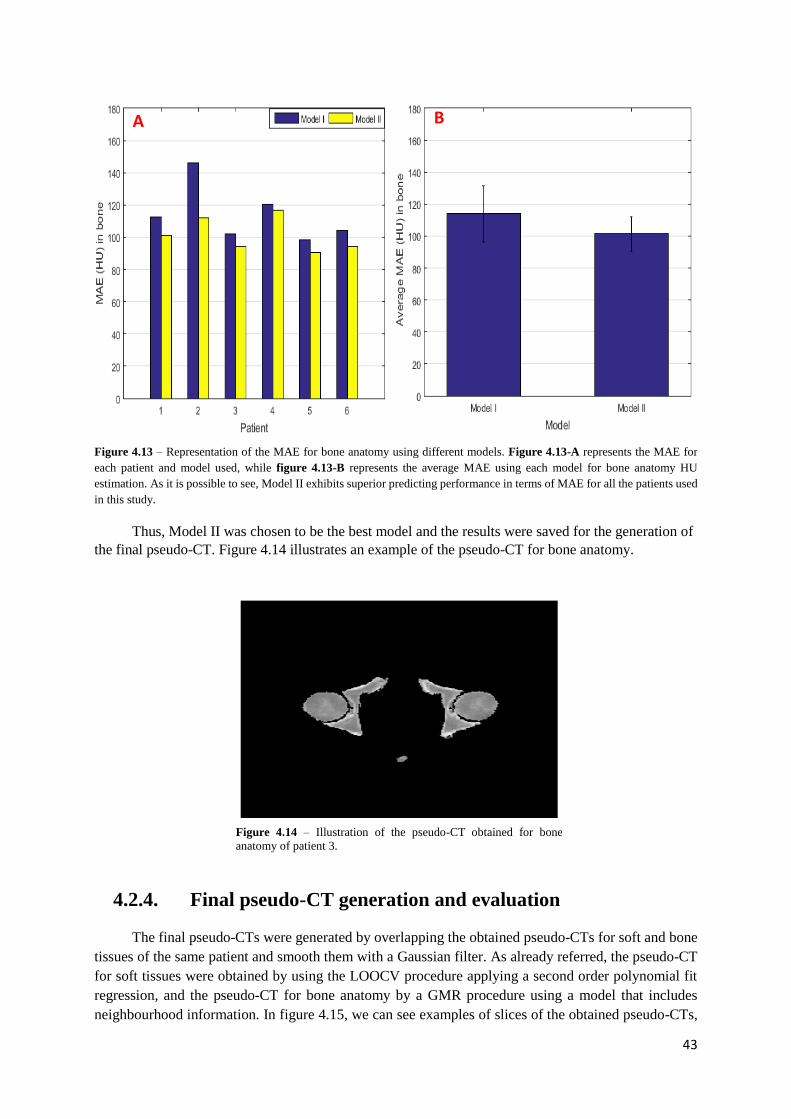
43

Thus, Model II was chosen to be the best model and the results were saved for the generation of

the final pseudo-CT. Figure 4.14 illustrates an example of the pseudo-CT for bone anatomy.

4.2.4. Final pseudo-CT generation and evaluation

The final pseudo-CTs were generated by overlapping the obtained pseudo-CTs for soft and bone

tissues of the same patient and smooth them with a Gaussian filter. As already referred, the pseudo-CT

for soft tissues were obtained by using the LOOCV procedure applying a second order polynomial fit

regression, and the pseudo-CT for bone anatomy by a GMR procedure using a model that includes

neighbourhood information. In figure 4.15, we can see examples of slices of the obtained pseudo-CTs,

B A

Figure 4.13 – Representation of the MAE for bone anatomy using different models. Figure 4.13-A represents the MAE for

each patient and model used, while figure 4.13-B represents the average MAE using each model for bone anatomy HU

estimation. As it is possible to see, Model II exhibits superior predicting performance in terms of MAE for all the patients used

in this study.

Figure 4.14 – Illustration of the pseudo-CT obtained for bone

anatomy of patient 3.

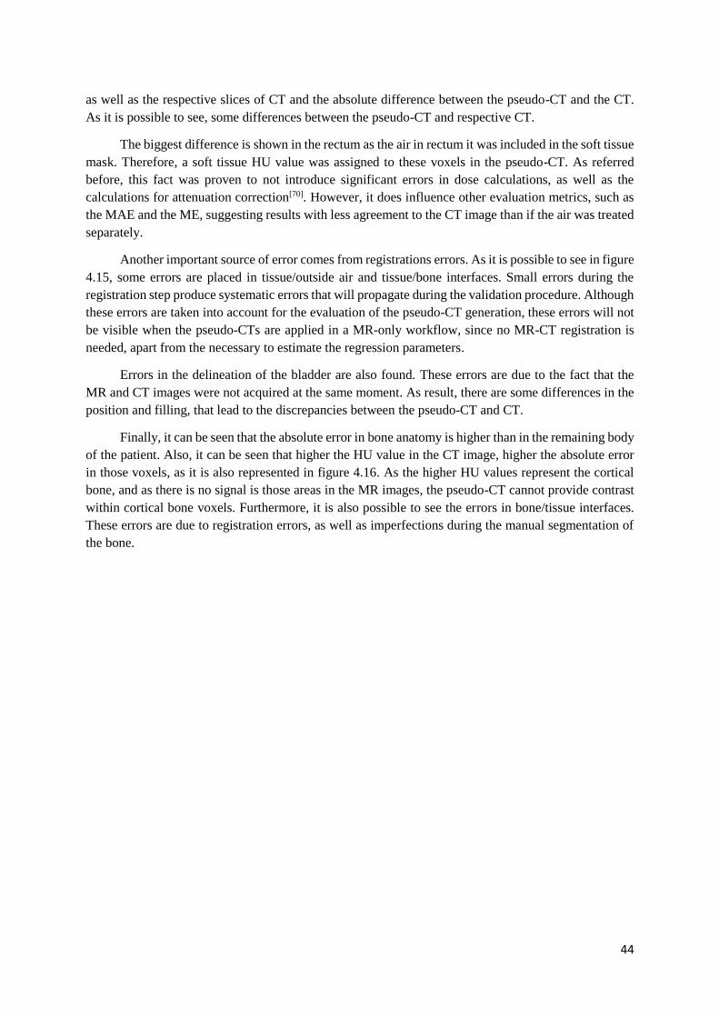
44

as well as the respective slices of CT and the absolute difference between the pseudo-CT and the CT.

As it is possible to see, some differences between the pseudo-CT and respective CT.

The biggest difference is shown in the rectum as the air in rectum it was included in the soft tissue

mask. Therefore, a soft tissue HU value was assigned to these voxels in the pseudo-CT. As referred

before, this fact was proven to not introduce significant errors in dose calculations, as well as the

calculations for attenuation correction[70]. However, it does influence other evaluation metrics, such as

the MAE and the ME, suggesting results with less agreement to the CT image than if the air was treated

separately.

Another important source of error comes from registrations errors. As it is possible to see in figure

4.15, some errors are placed in tissue/outside air and tissue/bone interfaces. Small errors during the

registration step produce systematic errors that will propagate during the validation procedure. Although

these errors are taken into account for the evaluation of the pseudo-CT generation, these errors will not

be visible when the pseudo-CTs are applied in a MR-only workflow, since no MR-CT registration is

needed, apart from the necessary to estimate the regression parameters.

Errors in the delineation of the bladder are also found. These errors are due to the fact that the

MR and CT images were not acquired at the same moment. As result, there are some differences in the

position and filling, that lead to the discrepancies between the pseudo-CT and CT.

Finally, it can be seen that the absolute error in bone anatomy is higher than in the remaining body

of the patient. Also, it can be seen that higher the HU value in the CT image, higher the absolute error

in those voxels, as it is also represented in figure 4.16. As the higher HU values represent the cortical

bone, and as there is no signal is those areas in the MR images, the pseudo-CT cannot provide contrast

within cortical bone voxels. Furthermore, it is also possible to see the errors in bone/tissue interfaces.

These errors are due to registration errors, as well as imperfections during the manual segmentation of

the bone.

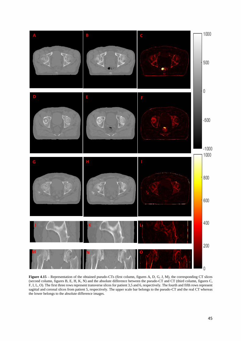
45

A B C

D

O N M

L K J

I H G

F E

Figure 4.15 – Representation of the obtained pseudo-CTs (first column, figures A, D, G, J, M), the corresponding CT slices

(second column, figures B, E, H, K, N) and the absolute difference between the pseudo-CT and CT (third column, figures C,

F, I, L, O). The first three rows represent transverse slices for patient 3,5 and 6, respectively. The fourth and fifth rows represent

sagittal and coronal slices from patient 5, respectively. The upper scale bar belongs to the pseudo-CT and the real CT whereas

the lower belongs to the absolute difference images.

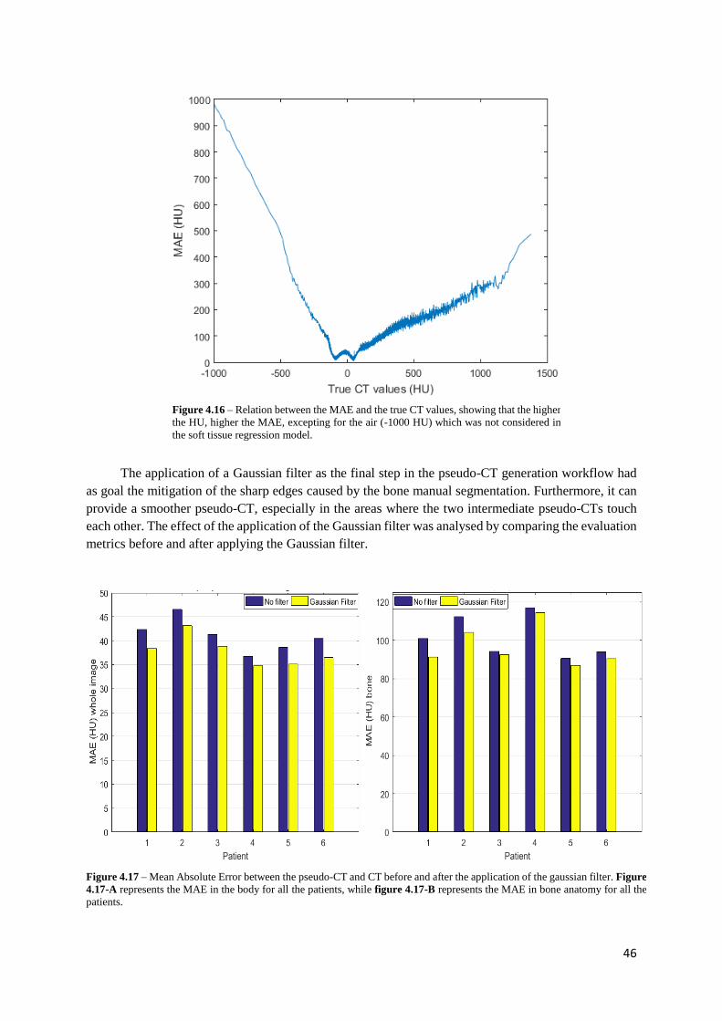
46

The application of a Gaussian filter as the final step in the pseudo-CT generation workflow had

as goal the mitigation of the sharp edges caused by the bone manual segmentation. Furthermore, it can

provide a smoother pseudo-CT, especially in the areas where the two intermediate pseudo-CTs touch

each other. The effect of the application of the Gaussian filter was analysed by comparing the evaluation

metrics before and after applying the Gaussian filter.

Figure 4.16 – Relation between the MAE and the true CT values, showing that the higher

the HU, higher the MAE, excepting for the air (-1000 HU) which was not considered in

the soft tissue regression model.

Figure 4.17 – Mean Absolute Error between the pseudo-CT and CT before and after the application of the gaussian filter. Figure

4.17-A represents the MAE in the body for all the patients, while figure 4.17-B represents the MAE in bone anatomy for all the

patients.

47

Figure 4.17-A represents the MAE in the body of the patient before and after applying the

Gaussian filter, while figure 4.17-B represents the MAE in bone anatomy in the same conditions. As it

can be seen, the application of the Gaussian filter results in a lower MAE for the whole body of the

patient, as well as for the bone anatomy. For the whole-body evaluation, an average MAE of 43.32 ±

4.01 HU was found before the application of the Gaussian filter, while after an average MAE of 37.76

± 4.01 HU was obtained. Also, an average ME of -2.68 ± 6.32 HU was found after the application of

the Gaussian filter, meaning that there is small bias in the pseudo-CT estimation. For bone anatomy, an

average MAE of 101.49±10.80 HU was found before the application of the Gaussian filter, while after

an average MAE of 96.61±10.49 HU was obtained. The average ME after the application of the

Gaussian filter was -10.01±48.04 HU, meaning that the estimation of the HU in bone anatomy is

underestimated, mainly due to the presence of cortical bone.

The pseudo-CT was also evaluated using different evaluation metrics as the SSIM and the PSNR.

Figure 4.18-A represents the SSIM of the whole body of each patient before and after the application of

the Gaussian filter, while figure 4.18-B illustrates the PSNR under the same conditions. As it can be

seen in both figures, the application of the Gaussian filter results in higher values of SSIM and PSNR.

An average SSIM value of 0.90±0.01 was obtained before the application of the Gaussian filter, while

after its application an average SSIM value of 0.91±0.01 was obtained. This fact means that a higher

structural resemblance between the pseudo-CT and the respective CT after the application of the

Gaussian filter. In the same way, an average PSNR of 23.42±1.43 dB was found before applying the

filter, while after a higher average PSNR of 23.92±1.62 dB was obtained. These values of PSNR mean

that the reconstruction of the pseudo-CT is less affected by the corrupting errors when the Gaussian

filter is applied.

The higher performances in terms of MAE, SSIM and PSNR leads to the conclusion that the

application of the Gaussian filter can mitigate the sharp edges caused by the manual segmentation by

smoothing the interfaces between different tissue types. In this way, a smoother pseudo-CT is obtained.

Figure 4.18-A and figure 4.18-B – Representation of the obtained value for each patient of the SSIM and the PSNR,

respectively, before and after the application of the gaussian filter

48

Figure 4.19 represents the joint histogram between the true HU values and the predicted HU

values. The green line in this histogram represents the ideal case where the predicted HU values are

exactly the same as the true HU values. This green line means that the points above this line are

overestimated, while the points below this green are underestimated. Also, further the distance of each

point to the green line, higher the difference of that value to the true HU value. Analysing this joint

histogram, a good correlation between the predicted and true HU values may be found. Also, some of

the problems that were already discussed may be visible. It can be seen the presence of underestimation

of the higher HU values, corresponding to cortical bone, once the majority of the points in this area in

the joint histogram are below the green line. Also, it can be seen that the air in the CT image was

classified as soft tissue, as it was already discussed. Furthermore, the effect of misregistrations is here

represented by the horizontal deviations from the green line in the area of the soft tissue (-100 HU to

100 HU).

The full process of training and validation in the LOOCV had the duration of 6 minutes to perform

all the patients, excluding the manual segmentation of the bone. Specifically, the training phase lasted

for 5 minutes, while the validation phase only last 1 minute to be performed. The majority of the time

required is spent in the bone pseudo-CT generation, once the Gaussian mixture regression is

computationally much more expensive than a simple polynomial regression.

Figure 4.19 – Joint histogram between the true CT number and the predicted

CT number. The green line represents the ideal scenario where the pseudo-CT

is exactly equal to the real CT. Points below this line indicate a higher HU in

the real CT compared to the pseudo-CT, while points above indicate a higher

HU in the pseudo-CT compared to the real CT.

49

Chapter 5

Conclusions and Future Work

MRI is receiving a lot of attention due to its wide range of applications which can bring benefits

for techniques such as PET and RTP. However, the lack of correlation between the MR-signal and the

attenuation properties of the tissues necessary for calculating the attenuation correction in PET and doses

in RTP is a challenge that needs to be overcome to enable PET-MRI and MR-RTP procedures without

the use of a CT scan.

In this thesis, a novel pseudo-CT generation method for the pelvic area was developed relying on

the exploitation of prior knowledge of the characteristics of the MR signal formation and tissue

properties. This method is based on a dual-model regression approach, one for the soft tissues and

another one for the bone anatomy based on the water and fat signal and the T2* decay to construct the

pseudo-CT. The input of both models includes the fat fraction image, for the soft tissue regression

model, and the fat fraction, water and fat, and R2* images for the bone regression model. These images

were obtained from multi-gradient echo data, whereas the aim of the models was to accurately reproduce

the HU estimation as in a traditional CT scan, by constructing pseudo-CT images. Furthermore, it was

demonstrated that the inclusion of neighbourhood information, obtained by calculating the standard

deviation of each voxel in the 27-neighbourhood, in the regression model for the bone anatomy can

significantly improve the estimation of HU values in those areas.

The results obtained in this project present large improvements when compared to other voxel-

based methods used for the pelvic area. In this work, an average MAE of 37.76 ± 4.01 HU was obtained.

Kim et al. obtained a MAE of 75 HU using several different MR sequences[23], and Korhonen et al.

obtained a MAE of 125 HU, by using a T1/ T2* weighted MR sequence[70]. This fact proves the superior

predicting capability of this approach. Furthermore, it is possible to compare the results with anatomy-

based methods. Dowling et al. obtained a MAE of 40.5 HU[66], while Burgos et al. obtained a MAE of

42.9 HU. Burgos et al. also reported a MAE in bone around 100 HU[67]. These results are in the same

order in the same order as the ones that were obtained in the method here presented. Thus, it can be

concluded that this method allows the generation of a pseudo-CT for the pelvic area with better or

identical agreement with the real CT than the methods described in literature. However, the validation

in an independent and bigger training and validation group should be performed.

This method presents several advantages over other methods present in literature. First, no

registration is needed avoiding the ambiguities caused by registration errors, excepting for the

registration errors during the parameter estimation[66] [67]. Moreover, the entire set of features (water, fat,

fat fraction and R2* images) used in this method are obtained through post-processing of a single MR

scan, as opposed to multiple scans with different contrasts, which makes it robust against interscan

motion and renders the method fast[23]. Furthermore, the computational burden of this method may be

reduced in institutions who possess an integrated water-fat decomposition scheme provided by the

vendor. In this case, the water-fat decomposition algorithm may be replaced by the water and fat images

that are already reconstructed. Thus, the parameter estimation should be performed once per institution

and machine in order to overcome possible differences in the hardware and software used.

50

However, this method also presents some drawbacks. The major limitation of this method is that

the bone segmentation is performed manually, increasing the workload and preventing a fully automatic

clinical introduction of the method. This drawback is not exclusive of our method, since most voxel-

based methods present in literature also rely on manual segmentation[23] [70]. Another limitation of this

study is related to the R2* estimation, which is specific for the echo times used in this project. Although

it is expected that the method may be possible to apply with different echo times (requiring the parameter

estimation for each set of values used), this hypothesis still needs to be validated. At last, the number of

patients used in the training sets is relatively low. By increasing the number of patients in the training

set, it is expected to obtain more robust results.

Some improvements to the presented method can be done in order to obtain better results as well

as a fully automatic method. First, the acquisition of more data will provide more robust training sets

which it is expected to lead to a better HU values estimation.

Also, the inclusion of an automatic MRI bone segmentation method is necessary to turn this

method completely automatic and, therefore, can be used in clinical practice without requiring an extra

workload for the clinicians. Although, this is still an active area of research, the inclusion of an atlas

based segmentation of the bone or the construction of a shape model of the bone are possible solutions

to turn this method fully automatic[73] [74]. The resulting method would be a hybrid method, by combining

the anatomical information of the bone with the voxelwise conversion of the MR related features into

HU values.

Furthermore, the inclusion of other MR features into the bone regression model is possible,

allowing a better HU estimation in bone anatomy. Quantitative Susceptibility Mapping (QSM) is a post-

processing MR technique which allows the quantification of the susceptibility in different tissues[94] [95].

It is well known that susceptibility values are correlated with the bone mineral density[27]. In this way,

another variable may be added to the model. Furthermore, recent advances in QSM techniques allow

the quantification of susceptibility values in air and cortical bone even if no signal is available in these

areas[96]. As cortical bone and air present different susceptibility values, the segmentation of these tissues

may be possible without requiring any anatomic information[97]. Also, it may be possible with the

inclusion of this variable that the GMR may be applied to the whole image, allowing the distinction

between bone, fat, water and air, and therefore obtain a more accurate pseudo-CT.

At last, it was recently demonstrated that the use of a multi-gradient echo scheme, as well as

water-fat reconstructions were useful for the identification of fiducial markers in prostate that are

necessary for radiotherapy[98] [99]. In this way, the development of a complete MR-only RTP procedure

may be possible only using the features used in this project.

As a final conclusion, we envision that this method may facilitate the development of PET-MRI

and MR-only RTP workflows by providing a method to completely replace the use of CT acquisitions,

reducing costs associated with its acquisition and sparing the patient to radiation exposure.

51

References

[1] P. E. Kinahan, B. H. Hasegawa, and T. Beyer, ‘X-ray-based attenuation correction for positron

emission tomography/computed tomography scanners’, Semin. Nucl. Med., vol. 33, no. 3, pp. 166–

179, Jul. 2003.

[2] W. Skrzyński, S. Zielińska-Dabrowska, M. Wachowicz, W. Slusarczyk-Kacprzyk, P. F.

Kukołowicz, and W. Bulski, ‘Computed tomography as a source of electron density information

for radiation treatment planning’, Strahlenther. Onkol. Organ Dtsch. Rontgengesellschaft Al, vol.

186, no. 6, pp. 327–333, Jun. 2010.

[3] E. Teplinsky, A. Pujara, F. J. Esteva, L. Moy, A. Melsaether, and K. L. Jhaveri, ‘Detection of

metastases in breast cancer: Is whole body PET/MR better than PET/CT?’, J. Clin. Oncol., vol.

32, no. 26_suppl, pp. 15–15, Sep. 2014.

[4] A. Afshar-Oromieh et al., ‘Comparison of PET/CT and PET/MRI hybrid systems using a 68Ga-

labelled PSMA ligand for the diagnosis of recurrent prostate cancer: initial experience’, Eur. J.

Nucl. Med. Mol. Imaging, vol. 41, no. 5, pp. 887–897, May 2014.

[5] M. Souvatzoglou et al., ‘Comparison of integrated whole-body [11C]choline PET/MR with

PET/CT in patients with prostate cancer’, Eur. J. Nucl. Med. Mol. Imaging, vol. 40, no. 10, pp.

1486–1499, Oct. 2013.

[6] J. C. Dickson, C. O’Meara, and A. Barnes, ‘A comparison of CT- and MR-based attenuation

correction in neurological PET’, Eur. J. Nucl. Med. Mol. Imaging, vol. 41, no. 6, pp. 1176–1189,

Jun. 2014.

[7] A. Samarin et al., ‘PET/MR imaging of bone lesions--implications for PET quantification from

imperfect attenuation correction’, Eur. J. Nucl. Med. Mol. Imaging, vol. 39, no. 7, pp. 1154–1160,

Jul. 2012.

[8] D. Izquierdo-Garcia et al., ‘Comparison of MR-based attenuation correction and CT-based

attenuation correction of whole-body PET/MR imaging’, Eur. J. Nucl. Med. Mol. Imaging, vol.

41, no. 8, pp. 1574–1584, Aug. 2014.

[9] S. Hitz et al., ‘Systematic Comparison of the Performance of Integrated Whole-Body PET/MR

Imaging to Conventional PET/CT for 18F-FDG Brain Imaging in Patients Examined for Suspected

Dementia’, J. Nucl. Med. Off. Publ. Soc. Nucl. Med., vol. 55, no. 6, pp. 923–931, Jun. 2014.

[10] M. Hofmann, B. Pichler, B. Schölkopf, and T. Beyer, ‘Towards quantitative PET/MRI: a review

of MR-based attenuation correction techniques’, Eur. J. Nucl. Med. Mol. Imaging, vol. 36 Suppl

1, pp. S93-104, Mar. 2009.

[11] A. Sciarra et al., ‘Advances in magnetic resonance imaging: how they are changing the

management of prostate cancer’, Eur. Urol., vol. 59, no. 6, pp. 962–977, Jun. 2011.

[12] V. S. Khoo and D. L. Joon, ‘New developments in MRI for target volume delineation in

radiotherapy’, Br. J. Radiol., vol. 79 Spec No 1, pp. S2-15, Sep. 2006.

[13] B. G. Fallone et al., ‘First MR images obtained during megavoltage photon irradiation from a

prototype integrated linac-MR system’, Med. Phys., vol. 36, no. 6, pp. 2084–2088, Jun. 2009.

[14] C. Rasch, R. Steenbakkers, and M. van Herk, ‘Target definition in prostate, head, and neck’,

Semin. Radiat. Oncol., vol. 15, no. 3, pp. 136–145, Jul. 2005.

[15] Prabhakar, ‘Comparison of computed tomography and magnetic resonance based target volume

in brain tumors’. [Online]. Available: http://www.cancerjournal.net/article.asp?issn=0973-

1482;year=2007;volume=3;issue=2;spage=121;epage=123;aulast=Prabhakar. [Accessed: 12-

Sep-2017].

52

[16] A. Fiorentino, R. Caivano, P. Pedicini, and V. Fusco, ‘Clinical target volume definition for

glioblastoma radiotherapy planning: magnetic resonance imaging and computed tomography’,

Clin. Transl. Oncol. Off. Publ. Fed. Span. Oncol. Soc. Natl. Cancer Inst. Mex., vol. 15, no. 9, pp.

754–758, Sep. 2013.

[17] K.-H. Su et al., ‘Generation of brain pseudo-CTs using an undersampled, single-acquisition UTE-

mDixon pulse sequence and unsupervised clustering’, Med. Phys., vol. 42, no. 8, pp. 4974–4986,

Aug. 2015.

[18] J. M. Edmund and T. Nyholm, ‘A review of substitute CT generation for MRI-only radiation

therapy’, Radiat. Oncol., vol. 12, p. 28, Jan. 2017.

[19] J. E. Holmes and G. M. Bydder, ‘MR imaging with ultrashort TE (UTE) pulse sequences: Basic

principles’, Radiography, vol. 11, no. 3, pp. 163–174, Aug. 2005.

[20] T. Nyholm and J. Jonsson, ‘Counterpoint: Opportunities and challenges of a magnetic resonance

imaging-only radiotherapy work flow’, Semin. Radiat. Oncol., vol. 24, no. 3, pp. 175–180, Jul.

2014.

[21] S.-H. Hsu, Y. Cao, K. Huang, M. Feng, and J. M. Balter, ‘Investigation of a method for generating

synthetic CT models from MRI scans of the head and neck for radiation therapy’, Phys. Med. Biol.,

vol. 58, no. 23, pp. 8419–8435, Dec. 2013.

[22] A. Johansson, M. Karlsson, and T. Nyholm, ‘CT substitute derived from MRI sequences with

ultrashort echo time’, Med. Phys., vol. 38, no. 5, pp. 2708–2714, May 2011.

[23] J. Kim, C. Glide-Hurst, A. Doemer, N. Wen, B. Movsas, and I. J. Chetty, ‘Implementation of a

novel algorithm for generating synthetic CT images from magnetic resonance imaging data sets

for prostate cancer radiation therapy’, Int. J. Radiat. Oncol. Biol. Phys., vol. 91, no. 1, pp. 39–47,

Jan. 2015.

[24] M. H. Arokoski, J. P. A. Arokoski, P. Vainio, L. H. Niemitukia, H. Kröger, and J. S. Jurvelin,

‘Comparison of DXA and MRI methods for interpreting femoral neck bone mineral density’, J.

Clin. Densitom. Off. J. Int. Soc. Clin. Densitom., vol. 5, no. 3, pp. 289–296, 2002.

[25] V. Keereman, Y. Fierens, T. Broux, Y. De Deene, M. Lonneux, and S. Vandenberghe, ‘MRI-based

attenuation correction for PET/MRI using ultrashort echo time sequences’, J. Nucl. Med. Off. Publ.

Soc. Nucl. Med., vol. 51, no. 5, pp. 812–818, May 2010.

[26] J.-P. Kühn et al., ‘Proton-density fat fraction and simultaneous R2* estimation as an MRI tool for

assessment of osteoporosis’, Eur. Radiol., vol. 23, no. 12, pp. 3432–3439, Dec. 2013.

[27] A. V. Dimov, Z. Liu, P. Spincemaille, M. R. Prince, J. Du, and Y. Wang, ‘Bone quantitative

susceptibility mapping using a chemical species-specific R2* signal model with ultrashort and

conventional echo data’, Magn. Reson. Med., Mar. 2017.

[28] S. Lee, C. K. Chung, S. H. Oh, and S. B. Park, ‘Correlation between Bone Mineral Density

Measured by Dual-Energy X-Ray Absorptiometry and Hounsfield Units Measured by Diagnostic

CT in Lumbar Spine’, J. Korean Neurosurg. Soc., vol. 54, no. 5, pp. 384–389, Nov. 2013.

[29] P. Hoskin and V. Goh, Eds., Radiotherapy in Practice - Imaging. Oxford, New York: Oxford

University Press, 2010.

[30] J. T. Bushberg, J. A. Seibert, E. M. Leidholdt, and J. M. Boone, The Essential Physics of Medical

Imaging. Lippincott Williams & Wilkins, 2011.

[31] W. R. Hendee and E. R. Ritenour, Medical Imaging Physics. John Wiley & Sons, 2003.

[32] M. Goitein, Radiation Oncology: A Physicist’s-Eye View. Springer Science & Business Media,

2007.

[33] A. Oppelt, Imaging Systems for Medical Diagnostics: Fundamentals, Technical Solutions and

Applications for Systems Applying Ionizing Radiation, Nuclear Magnetic Resonance and

Ultrasound. John Wiley & Sons, 2011.

53

[34] U. Schneider, E. Pedroni, and A. Lomax, ‘The calibration of CT Hounsfield units for radiotherapy

treatment planning’, Phys. Med. Biol., vol. 41, no. 1, pp. 111–124, Jan. 1996.

[35] H. Günther, NMR Spectroscopy: Basic Principles, Concepts and Applications in Chemistry, 3

edition. Weinheim: Wiley-VCH, 2013.

[36] A. Ribeiro, ‘Bone recognition in UTE MR images by artificial neural networks for attenuation

correction of brain imaging in MR/PET scanners’, MSc, University of Lisbon, Lisbon, 2012.

[37] M. A. Brown and R. C. Semelka, MRI: Basic Principles and Applications, 4 edition. Hoboken,

N.J: Wiley-Blackwell, 2010.

[38] D. Weishaupt, V. D. Koechli, and B. Marincek, How does MRI work?: An Introduction to the

Physics and Function of Magnetic Resonance Imaging, 2nd edition. Berlin ; New York: Springer,

2008.

[39] D. W. McRobbie, E. A. Moore, M. J. Graves, and M. R. Prince, MRI from Picture to Proton, 2

edition. Cambridge, UK ; New York: Cambridge University Press, 2007.

[40] T. A. Bley, O. Wieben, C. J. François, J. H. Brittain, and S. B. Reeder, ‘Fat and water magnetic

resonance imaging’, J. Magn. Reson. Imaging JMRI, vol. 31, no. 1, pp. 4–18, Jan. 2010.

[41] A. Haase, J. Frahm, W. Hänicke, and D. Matthaei, ‘1H NMR chemical shift selective (CHESS)

imaging’, Phys. Med. Biol., vol. 30, no. 4, pp. 341–344, Apr. 1985.

[42] G. M. Bydder, J. M. Pennock, R. E. Steiner, S. Khenia, J. A. Payne, and I. R. Young, ‘The short

TI inversion recovery sequence--an approach to MR imaging of the abdomen’, Magn. Reson.

Imaging, vol. 3, no. 3, pp. 251–254, 1985.

[43] M. Dousset et al., ‘Short TI inversion-recovery imaging of the liver: pulse-sequence optimization

and comparison with spin-echo imaging’, Radiology, vol. 171, no. 2, pp. 327–333, May 1989.

[44] J. Ma, ‘Dixon techniques for water and fat imaging’, J. Magn. Reson. Imaging JMRI, vol. 28, no.

3, pp. 543–558, Sep. 2008.

[45] G. Brix, S. Heiland, M. E. Bellemann, T. Koch, and W. J. Lorenz, ‘MR imaging of fat-containing

tissues: valuation of two quantitative imaging techniques in comparison with localized proton

spectroscopy’, Magn. Reson. Imaging, vol. 11, no. 7, pp. 977–991, 1993.

[46] Q. S. Xiang and L. An, ‘Water-fat imaging with direct phase encoding’, J. Magn. Reson. Imaging

JMRI, vol. 7, no. 6, pp. 1002–1015, Dec. 1997.

[47] W. T. Dixon, ‘Simple proton spectroscopic imaging’, Radiology, vol. 153, no. 1, pp. 189–194,

Oct. 1984.

[48] G. H. Glover and E. Schneider, ‘Three-point Dixon technique for true water/fat decomposition

with B0 inhomogeneity correction’, Magn. Reson. Med., vol. 18, no. 2, pp. 371–383, Apr. 1991.

[49] D. C. Ghiglia and M. D. Pritt, Two-Dimensional Phase Unwrapping: Theory, Algorithms, and

Software, 1 edition. New York: Wiley-Interscience, 1998.

[50] S. Moon-Ho Song, S. Napel, N. J. Pelc, and G. H. Glover, ‘Phase unwrapping of MR phase images

using Poisson equation’, IEEE Trans. Image Process. Publ. IEEE Signal Process. Soc., vol. 4, no.

5, pp. 667–676, 1995.

[51] S. B. Reeder et al., ‘Iterative decomposition of water and fat with echo asymmetry and least-

squares estimation (IDEAL): application with fast spin-echo imaging’, Magn. Reson. Med., vol.

54, no. 3, pp. 636–644, Sep. 2005.

[52] H. Yu, S. B. Reeder, A. Shimakawa, J. H. Brittain, and N. J. Pelc, ‘Field map estimation with a

region growing scheme for iterative 3-point water-fat decomposition’, Magn. Reson. Med., vol.

54, no. 4, pp. 1032–1039, Oct. 2005.

[53] H. Yu et al., ‘Combination of complex-based and magnitude-based multiecho water-fat separation

for accurate quantification of fat-fraction’, Magn. Reson. Med., vol. 66, no. 1, pp. 199–206, Jul.

2011.

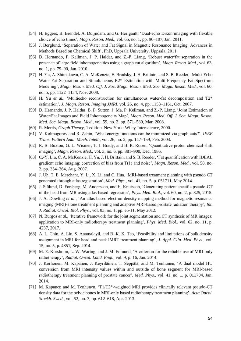
54

[54] H. Eggers, B. Brendel, A. Duijndam, and G. Herigault, ‘Dual-echo Dixon imaging with flexible

choice of echo times’, Magn. Reson. Med., vol. 65, no. 1, pp. 96–107, Jan. 2011.

[55] J. Berglund, ‘Separation of Water and Fat Signal in Magnetic Resonance Imaging: Advances in

Methods Based on Chemical Shift’, PhD, Uppsala University, Uppsala, 2011.

[56] D. Hernando, P. Kellman, J. P. Haldar, and Z.-P. Liang, ‘Robust water/fat separation in the

presence of large field inhomogeneities using a graph cut algorithm’, Magn. Reson. Med., vol. 63,

no. 1, pp. 79–90, Jan. 2010.

[57] H. Yu, A. Shimakawa, C. A. McKenzie, E. Brodsky, J. H. Brittain, and S. B. Reeder, ‘Multi-Echo

Water-Fat Separation and Simultaneous R2* Estimation with Multi-Frequency Fat Spectrum

Modeling’, Magn. Reson. Med. Off. J. Soc. Magn. Reson. Med. Soc. Magn. Reson. Med., vol. 60,

no. 5, pp. 1122–1134, Nov. 2008.

[58] H. Yu et al., ‘Multiecho reconstruction for simultaneous water-fat decomposition and T2*

estimation’, J. Magn. Reson. Imaging JMRI, vol. 26, no. 4, pp. 1153–1161, Oct. 2007.

[59] D. Hernando, J. P. Haldar, B. P. Sutton, J. Ma, P. Kellman, and Z.-P. Liang, ‘Joint Estimation of

Water/Fat Images and Field Inhomogeneity Map’, Magn. Reson. Med. Off. J. Soc. Magn. Reson.

Med. Soc. Magn. Reson. Med., vol. 59, no. 3, pp. 571–580, Mar. 2008.

[60] R. Merris, Graph Theory, 1 edition. New York: Wiley-Interscience, 2000.

[61] V. Kolmogorov and R. Zabin, ‘What energy functions can be minimized via graph cuts?’, IEEE

Trans. Pattern Anal. Mach. Intell., vol. 26, no. 2, pp. 147–159, Feb. 2004.

[62] R. B. Buxton, G. L. Wismer, T. J. Brady, and B. R. Rosen, ‘Quantitative proton chemical-shift

imaging’, Magn. Reson. Med., vol. 3, no. 6, pp. 881–900, Dec. 1986.

[63] C.-Y. Liu, C. A. McKenzie, H. Yu, J. H. Brittain, and S. B. Reeder, ‘Fat quantification with IDEAL

gradient echo imaging: correction of bias from T(1) and noise’, Magn. Reson. Med., vol. 58, no.

2, pp. 354–364, Aug. 2007.

[64] J. Uh, T. E. Merchant, Y. Li, X. Li, and C. Hua, ‘MRI-based treatment planning with pseudo CT

generated through atlas registration’, Med. Phys., vol. 41, no. 5, p. 051711, May 2014.

[65] J. Sjölund, D. Forsberg, M. Andersson, and H. Knutsson, ‘Generating patient specific pseudo-CT

of the head from MR using atlas-based regression’, Phys. Med. Biol., vol. 60, no. 2, p. 825, 2015.

[66] J. A. Dowling et al., ‘An atlas-based electron density mapping method for magnetic resonance

imaging (MRI)-alone treatment planning and adaptive MRI-based prostate radiation therapy’, Int.

J. Radiat. Oncol. Biol. Phys., vol. 83, no. 1, pp. e5-11, May 2012.

[67] N. Burgos et al., ‘Iterative framework for the joint segmentation and CT synthesis of MR images:

application to MRI-only radiotherapy treatment planning’, Phys. Med. Biol., vol. 62, no. 11, p.

4237, 2017.

[68] A. L. Chin, A. Lin, S. Anamalayil, and B.-K. K. Teo, ‘Feasibility and limitations of bulk density

assignment in MRI for head and neck IMRT treatment planning’, J. Appl. Clin. Med. Phys., vol.

15, no. 5, p. 4851, Sep. 2014.

[69] M. E. Korsholm, L. W. Waring, and J. M. Edmund, ‘A criterion for the reliable use of MRI-only

radiotherapy’, Radiat. Oncol. Lond. Engl., vol. 9, p. 16, Jan. 2014.

[70] J. Korhonen, M. Kapanen, J. Keyriläinen, T. Seppälä, and M. Tenhunen, ‘A dual model HU

conversion from MRI intensity values within and outside of bone segment for MRI-based

radiotherapy treatment planning of prostate cancer’, Med. Phys., vol. 41, no. 1, p. 011704, Jan.

2014.

[71] M. Kapanen and M. Tenhunen, ‘T1/T2*-weighted MRI provides clinically relevant pseudo-CT

density data for the pelvic bones in MRI-only based radiotherapy treatment planning’, Acta Oncol.

Stockh. Swed., vol. 52, no. 3, pp. 612–618, Apr. 2013.

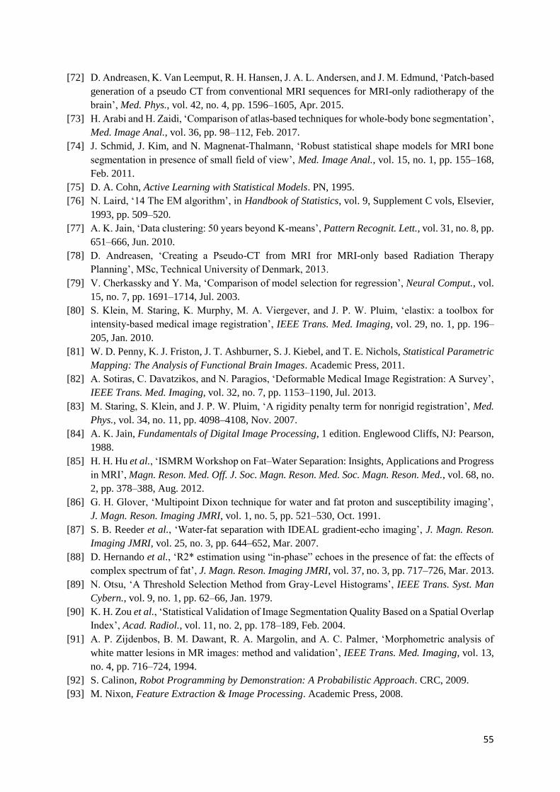
55

[72] D. Andreasen, K. Van Leemput, R. H. Hansen, J. A. L. Andersen, and J. M. Edmund, ‘Patch-based

generation of a pseudo CT from conventional MRI sequences for MRI-only radiotherapy of the

brain’, Med. Phys., vol. 42, no. 4, pp. 1596–1605, Apr. 2015.

[73] H. Arabi and H. Zaidi, ‘Comparison of atlas-based techniques for whole-body bone segmentation’,

Med. Image Anal., vol. 36, pp. 98–112, Feb. 2017.

[74] J. Schmid, J. Kim, and N. Magnenat-Thalmann, ‘Robust statistical shape models for MRI bone

segmentation in presence of small field of view’, Med. Image Anal., vol. 15, no. 1, pp. 155–168,

Feb. 2011.

[75] D. A. Cohn, Active Learning with Statistical Models. PN, 1995.

[76] N. Laird, ‘14 The EM algorithm’, in Handbook of Statistics, vol. 9, Supplement C vols, Elsevier,

1993, pp. 509–520.

[77] A. K. Jain, ‘Data clustering: 50 years beyond K-means’, Pattern Recognit. Lett., vol. 31, no. 8, pp.

651–666, Jun. 2010.

[78] D. Andreasen, ‘Creating a Pseudo-CT from MRI fror MRI-only based Radiation Therapy

Planning’, MSc, Technical University of Denmark, 2013.

[79] V. Cherkassky and Y. Ma, ‘Comparison of model selection for regression’, Neural Comput., vol.

15, no. 7, pp. 1691–1714, Jul. 2003.

[80] S. Klein, M. Staring, K. Murphy, M. A. Viergever, and J. P. W. Pluim, ‘elastix: a toolbox for

intensity-based medical image registration’, IEEE Trans. Med. Imaging, vol. 29, no. 1, pp. 196–

205, Jan. 2010.

[81] W. D. Penny, K. J. Friston, J. T. Ashburner, S. J. Kiebel, and T. E. Nichols, Statistical Parametric

Mapping: The Analysis of Functional Brain Images. Academic Press, 2011.

[82] A. Sotiras, C. Davatzikos, and N. Paragios, ‘Deformable Medical Image Registration: A Survey’,

IEEE Trans. Med. Imaging, vol. 32, no. 7, pp. 1153–1190, Jul. 2013.

[83] M. Staring, S. Klein, and J. P. W. Pluim, ‘A rigidity penalty term for nonrigid registration’, Med.

Phys., vol. 34, no. 11, pp. 4098–4108, Nov. 2007.

[84] A. K. Jain, Fundamentals of Digital Image Processing, 1 edition. Englewood Cliffs, NJ: Pearson,

1988.

[85] H. H. Hu et al., ‘ISMRM Workshop on Fat–Water Separation: Insights, Applications and Progress

in MRI’, Magn. Reson. Med. Off. J. Soc. Magn. Reson. Med. Soc. Magn. Reson. Med., vol. 68, no.

2, pp. 378–388, Aug. 2012.

[86] G. H. Glover, ‘Multipoint Dixon technique for water and fat proton and susceptibility imaging’,

J. Magn. Reson. Imaging JMRI, vol. 1, no. 5, pp. 521–530, Oct. 1991.

[87] S. B. Reeder et al., ‘Water-fat separation with IDEAL gradient-echo imaging’, J. Magn. Reson.

Imaging JMRI, vol. 25, no. 3, pp. 644–652, Mar. 2007.

[88] D. Hernando et al., ‘R2* estimation using “in-phase” echoes in the presence of fat: the effects of

complex spectrum of fat’, J. Magn. Reson. Imaging JMRI, vol. 37, no. 3, pp. 717–726, Mar. 2013.

[89] N. Otsu, ‘A Threshold Selection Method from Gray-Level Histograms’, IEEE Trans. Syst. Man

Cybern., vol. 9, no. 1, pp. 62–66, Jan. 1979.

[90] K. H. Zou et al., ‘Statistical Validation of Image Segmentation Quality Based on a Spatial Overlap

Index’, Acad. Radiol., vol. 11, no. 2, pp. 178–189, Feb. 2004.

[91] A. P. Zijdenbos, B. M. Dawant, R. A. Margolin, and A. C. Palmer, ‘Morphometric analysis of

white matter lesions in MR images: method and validation’, IEEE Trans. Med. Imaging, vol. 13,

no. 4, pp. 716–724, 1994.

[92] S. Calinon, Robot Programming by Demonstration: A Probabilistic Approach. CRC, 2009.

[93] M. Nixon, Feature Extraction & Image Processing. Academic Press, 2008.

56

[94] Y. Wang and T. Liu, ‘Quantitative susceptibility mapping (QSM): Decoding MRI data for a tissue

magnetic biomarker’, Magn. Reson. Med., vol. 73, no. 1, pp. 82–101, Jan. 2015.

[95] J. R. Reichenbach, F. Schweser, B. Serres, and A. Deistung, ‘Quantitative Susceptibility Mapping:

Concepts and Applications’, Clin. Neuroradiol., vol. 25 Suppl 2, pp. 225–230, Oct. 2015.

[96] Z. Liu, Y. Kee, D. Zhou, Y. Wang, and P. Spincemaille, ‘Preconditioned total field inversion (TFI)

method for quantitative susceptibility mapping’, Magn. Reson. Med., vol. 78, no. 1, pp. 303–315,

Jul. 2017.

[97] S. Buch, S. Liu, Y. Ye, Y.-C. N. Cheng, J. Neelavalli, and E. M. Haacke, ‘Susceptibility mapping

of air, bone, and calcium in the head’, Magn. Reson. Med., vol. 73, no. 6, pp. 2185–2194, Jun.

2015.

[98] M. Kapanen, J. Collan, A. Beule, T. Seppälä, K. Saarilahti, and M. Tenhunen, ‘Commissioning of

MRI-only based treatment planning procedure for external beam radiotherapy of prostate’, Magn.

Reson. Med., vol. 70, no. 1, pp. 127–135, Jul. 2013.

[99] M. Maspero et al., ‘Evaluation of an automatic MR-based gold fiducial marker localisation method

for MR-only prostate radiotherapy’, Phys. Med. Biol., Aug. 2017.

57

Appendix

Appendix I

This appendix presents the MATLAB list of input parameters for the water-fat decomposition

algorithm used in this project.

algoParams.species(1).name = 'water';

algoParams.species(1).frequency = 0;

algoParams.species(1).relAmps = 1;

algoParams.species(2).name = 'fat';

algoParams.species(2).frequency = [-3.80, -3.40, -2.60, -1.94, -

0.39, 0.60];

algoParams.species(2).relAmps = [0.087 0.693 0.128 0.004 0.039

0.048];

algoParams.size_clique = 1; algoParams.range_r2star = [0 0]; % Range

of R2* values

algoParams.NUM_R2STARS = 1; % Number of R2* values for quantization

algoParams.range_fm = [-700 700]; % Range of field map values

algoParams.NUM_FMS = 301; % Number of field map values to discretize

algoParams.NUM_ITERS = 40; % Number of graph cut iterations

algoParams.SUBSAMPLE =4; % Spatial subsampling for field map

estimation (for speed)

algoParams.DO_OT = 0; % 0,1 flag to enable optimization transfer

descent (final stage of field map estimation)

algoParams.LMAP_POWER = 2; % Spatially-varying regularization (2

gives ~ uniformn resolution)

algoParams.lambda = 0.05; % Regularization parameter

algoParams.LMAP_EXTRA = 0.02; % More smoothing for low-signal

regions

algoParams.TRY_PERIODIC_RESIDUAL = 0;

MR-based pseudo-CT generation using water-fat...

Documents

Transcript of MR-based pseudo-CT generation using water-fat...