EVENT BY EVENT AVERAGES IN HEAVY ION COLLISIONS

M. J. TANNENBAUM and J. T. MITCHELL Department of Physics, 510c, Brookhaven National Laboratory,

Upton, NY 11973-5000 , USA

'

.. ·• ';

' · .

.

NA49 (Pb+Pb, CERN) , PHENIX and STAR (Au+Au, BNL) have presented measurements of the event-by-event average PT (denoted MPT) in relativistic heavy ion collisions. Event-by­event averages are most useful to resolve the case of two or several classes of events with e.g. different temperature parameters. The distribution of MPT is discussed, with emphasis on the case of statistically independent emission according to the semi-inclusive PT and charged multiplicity distributions. Deviations from statistically independent emission are quantified in terms of a simple two component model, with the individual components being Gamma distributions.

1 Semi-Inclusive Distributions

In p-p and heavy ion collisions, the semi-inclusive distributions of charged multiplicity, n, and transverse momentum, pr, for a given centrality class (or impact parameter) , summing over all events in a class, are typically Negative Binomial Distributions (NBD) and Gamma Distribu­tions, respectively. l ,2 The NBD is the first departure from a Poisson distribution (for repeated independent trials, each with the same probability for a given outcome) which forms the basis of most physicist's 'intuition' for the statistics of random processes. The NBD allows some correlation, which is represented by a parameter parameter, l/k, which is zero for a Poisson distribution:

1 k

( 1 )

where (x) is the mean and u� i s the variance (ux i s the standard deviation) of the quantity x : (2)

The Gamma distribution has particularly simple properties under convolutions and scale transformations and for these reasons has proved useful in the study of 'Er' distributions. 3 The

3 89

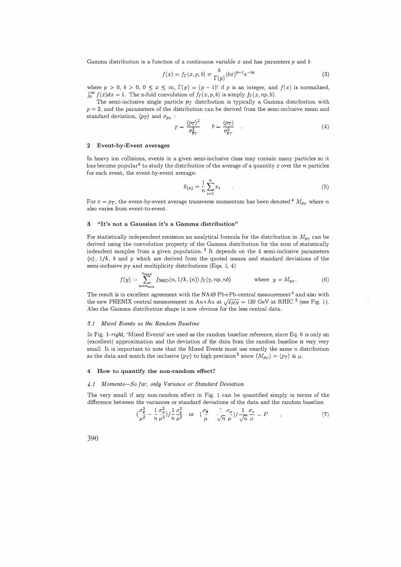
Gamma distribution is a function of a continuous variable x and has paramters p and b b

J(x) = fr (x, p , b) = r(p)

(bxr1e-bx (3)

where p > 0, b > 0, 0 ::; x ::; oo , r(p) = (p - 1) ! if p is an integer, and f(x) is normalized, J000 J(x)dx = l . The n-fold convolution of Jr(x, p, b) is simply fr(x, np, b) .

The semi-inclusive single particle PT distribution is typically a Gamma distribution with p = 2, and the parameters of the distribution can be derived from the semi-inclusive mean and standard deviation, (pr) and l7pr

(4)

2 Event-by-Event averages

In heavy ion collisions, events in a given semi-inclusive class may contain many particles so it has become popular4 to study the distribution of the average of a quantity x over the n particles for each event, the event-by-event average:

1 n X(n) = - L Xi (5)

n i=l

For x = py , the event-by-event average transverse momentum has been denoted 4 Mpr where n also varies from event-to-event.

3 "It's not a Gaussian it's a Gamma distribution"

For statistically independent emission an analytical formula for the distribution in Mpr can be derived using the convolution property of the Gamma distribution for the sum of statistically indendent samples from a given population. 2 It depends on the 4 semi-inclusive parameters (n) , l/k , b and p which are derived from the quoted means and standard deviations of the semi-inclusive PT and multiplicity distributions (Eqs. 1, 4)

J(y) = L fNBD (n, 1/k, (n)) Jr (Y, np, nb) where y = MPT . (6) n=nmin

The result is in excellent agreement with the NA49 Pb+ Pb-central measurement 4 and also with the new PHENIX central measurement in Au+Au at ftNN = 130 GeV at RHIC. 5 (see Fig. 1 ) . Also the Gamma distribution shape i s now obvious for the less central data.

3. 1 Mixed Events as the Random Baseline

In Fig. I-right, 'Mixed Events' are used as the random baseline reference, since Eq. 6 is only an (excellent) approximation and the deviation of the data from the random baseline is very very small. It is important to note that the Mixed Events must use exactly the same n distribution as the data and match the inclusive (pr) to high precision 5 since (Mpy) = (pr) = µ.

4 How to quantify the non-random effect?

4. 1 Moments-So far, only Variance or Standard Deviation

The very small if any non-random effect in Fig. 1 can be quantified simply in terms of the difference between the variances or standard deviations of the data and the random baseline:

390

2 1 2 1 2 ( x - - 17 x ) / - 17 x or µ2 n µ2 n µ2 (7)

IO' IO

0.3 0.4 0.5 M(pT) (GeV/c) "­,,.r---------,

'" '"

D 0.1 0.2 0.3 0.4 0.5 0.6 0.7 O.B 0.9 1 M,, (GeV/c)

N���·r-"--------� 0-5%

10'

10'

I I I

0 0.1 0.2 0.3 0.4 o.s 0.6 0.7 0.8 0.9 1 MPr (GeV/c) 10

'

10-20% 10

'

10'

o 0.1 0.2 o.3 o.4 o.s o.e 0.1 o.8 o.9 1 MPr (GeV/c)

N.,,."r-"--------� ,, 0·10"/o ,,.

10'

0 0.1 0.2 0.3 0.4 O.S 0.6 0.7 0.8 0.9 I Mp.(GeV!c}

20-30%

0 0.1 0.2 0.3 0.4 0.5 0,6 0.7 0.8 0.9 1 MPr(GeV/c) Figure 1: top left: Gamma Distribution for MPT (light line) compared to Gaussian with same (PT) and aMPT (darker line) for NA49 measurement. bottom left: Eq. 6 with PHENIX Au+Au central (top 53) data. right: PHENIX Au+Au data for 6..P = 1.02, 1'71 < 0.35 vs centrality. The dotted curves are mixed event distributions.

where for the random case a� = a�/n. Groups argue over whether the variance or standard deviation is better, however for small effects, these measures are equivalent:

In terms of F, the fractional difference of the data and random standard deviations, the PHENIX re­sults from Fig. 1 for centralities 0-53 ( (n) = 59.6) , 0-103 (53 .9 ) , 1 0-203 (36.6) and 20-303 (25 .0) are F = 0.019 ± 0.02 1 , 0.020 ± 0 .025, 0.021 ± 0.022, 0.018 ± 0.030 respectively, very small indeed, where the error is dominantly systematic. Note that F is independent of centrality, an effect also observed by STAR 6 (Fig. 2) , although for the same value of (n) the STAR preliminary result for F is 6 times larger than PHENIX, possibly due to the larger solid angle of the measurement in STAR (ti.ii? = 27!', 177 1 < 0.75) . A starkly different dependence of F on

Sl AR ;1,11,-Au ,:.,,,,.:: 130 (ic\' PRELIMINARY

0.05 0 o 1 oo 200 300 400 500 aoo 100 aoo

Fig. 2: Star results for F vs n, assuming

"fPr),.iat /µ2 = l/(np) = 1/2n, in which case the label on the y axis is equal to F

(8)

(n) is predicted for the case 7 of a temperature parameter T = l/b which varies event-by-event with mean and variance, (T) , a} , clearly not observed by either PHENIX or STAR:

p .

0'2 F = - ( (n) - l) _L__

2 (T)2

4.2 Two-Component Model for the MPT distribution

(9)

The event-by-event average is most useful to resolve the case of e.g. 2 classes of events with different PT distributions of which only one component appears on any given event. We represent

3 9 1

N .... ,.

,,.

,,

·-...... , __ _ ·, ... _'-... ...

'·.

Model A t.T=SO MeV

�' ·-....

N""""'"

,.• ··"·····.,,

,,.

N .... ,, " Model A

Model A t. T = SOMeV t.T=150 MeV

,,.

N ...... ,..

,,.

,,.

Model A t.T = 1 50 MeV .

= 1 . I

o 0.2 o.4 o.s o.8 1 1.2 1.4 1.s 1 . a 2 o 0.2 o.4 o.6 o.s 1 1.2 1.4 1.s 1.1 2 o 0.1 0.2 o.3 0.4 o.s o.8 0 1 0.a o.9 1 o 0.1 a.2 0.3 o., o.s o.6 0.1 o.a o.9 1 Mp, (GeV/c) M.,, (GeV/c) M,.. (GeV/c) M.,, (GeV/c)

N,,00,. N""""" N, N,1��i'-"-------� 10' Model B Model B

,,.

,,· ,,.

Model B !J.T:BO MeV

,,.

,,.

t. T = 20 MeV t. T = BO MeV

,,.

,,.

. , h

0 0,2 0.4 0.6 0.8 1 1.2 1.4 1 8 1.8 2 Mp, (GeV/c)

o 0.2 o.4 o.8 o.s 1 1.2 u 1.6 1.1' 2 o o.i 0.2 o.3 o.4 o.s o.s o.7 o.s o.9 , Mp, {GeVlc) Mp, (GeV/c)

0 0.1 0.2 0.3 0.4 0.5 0.6 0.7 08 0.9 1 Mp, (GeV/c)

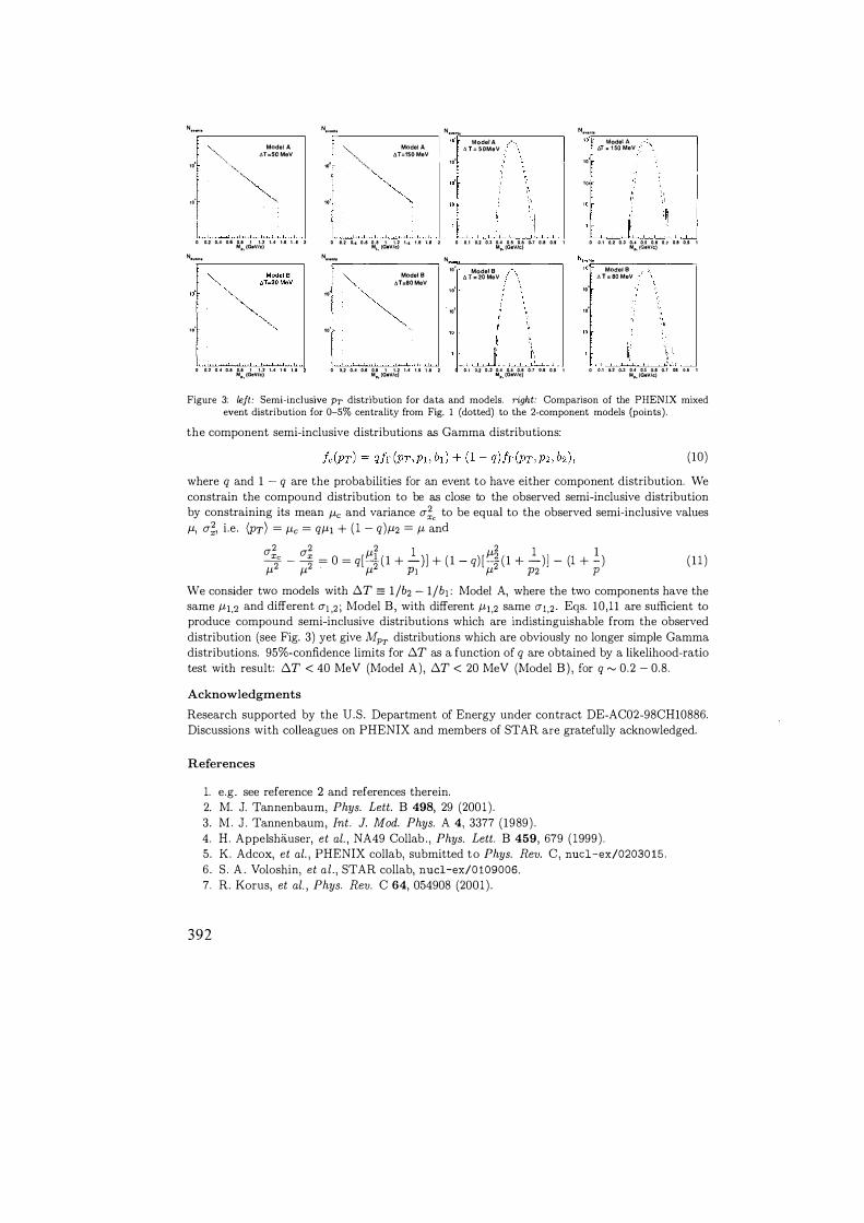
Figure 3: left: Semi-inclusive PT distribution for data and models. right: Comparison of the PHENIX mixed event distribution for 0-53 centrality from Fig. 1 (dotted) to the 2-component models (points) .

the component semi-inclusive distributions as Gamma distributions:

(10)

where q and 1 - q are the probabilities for an event to have either component distribution. We constrain the compound distribution to be as close to the observed semi-inclusive distribution by constraining its mean µc and variance u;, to be equal to the observed semi-inclusive values µ, u;, i .e. (pr) = µc = qµ1 + ( 1 - q)µ2 = µ and

u2 u2 µ2 1 µ2 1 1 � - ____'O. = 0 = q[__l. ( 1 + -)] + ( l - q) [ --2 ( 1 + -)] - (1 + - ) ( 1 1 ) µ2 µ2 . µ2 PI µ2 p2 p

We consider two models with 6,.T = l/b2 - l/b1 : Model A, where the two components have the same µ1,2 and different u1 ,2 ; Model B, with different µi,2 same u1,2 . Eqs. 10 ,11 are sufficient to produce compound semi-inclusive distributions which are indistinguishable from the observed distribution (see Fig. 3) yet give Mpr distributions which are obviously no longer simple Gamma distributions. 953-confidence limits for 6,.T as a function of q are obtained by a likelihood-ratio test with result: 6,.T < 40 MeV (Model A) , 6,.T < 20 MeV (Model B) , for q � 0.2 - 0.8 .

Acknowledgments

Research supported by the U.S. Department of Energy under contract DE-AC02-98CH10886. Discussions with colleagues on PHENIX and members of STAR are gratefully acknowledged.

References

1. e.g. see reference 2 and references therein. 2. M. J. Tannenbaum, Phys. Lett. B 498, 29 (2001 ) . 3. M. J . Tannenbaum, Int. J. Mod. Phys. A 4, 3377 (1989 ) . 4. H. Appelshauser, et al. , NA49 Collab. , Phys. Lett. B 459, 679 ( 1999 ) . 5. K. Adcox, et al. , PHENIX collab, submitted to Phys. Rev. C, nucl-ex/02030 15.

6 . S . A . Voloshin, et al . , STAR collab, nucl-ex/0 109006.

7. R. Korus, et al. , Phys. Rev. C 64, 054908 (2001 ) .

392