MPO 674 Lecture 20

3/26/15

3d-Var vs 4d-Var

Ensemble Kalman Filters

• Want flow-dependent, dynamical covariances• Several different types of Kalman filter exist, all of

which have a linear inference. Non-linear filters are too hard. Seek simple approximations ...

• Ensemble Kalman filters use Pf = Zf ZfT

Zf is an n x k matrix containing k ensemble perturbations (about a mean state) of length n.

Perturbation

Pf = Zf ZfT

(u’1)1 (u’1)2 (u’1)3

(v’1)1 (v’1)2 (v’1)3

(T’1)1 (T’1)2 (T’1)3

(p’1)1 (p’1)2 (p’1)3

(u’2)1 (u’2)2 (u’2)3

(v’2)1 (v’2)2 (v’2)3

(T’2)1 (T’2)2 (T’2)3

(p’2)1 (p’2)2 (p’2)3

(u’3)1 (u’3)2 (u’3)3

… … …

… … …

(u’1)1 (v’1)1 (T’1)1 (p’1)1 (u’2)1 (v’2)1 (T’2)1 (p’2)1 (u’3)1

(u’1)2 (v’1)2 (T’1)2 (p’1)2 (u’2)2 (v’2)2 (T’2)2 (p’2)2 (u’3)2

(u’1)3 (v’1)3 (T’1)3 (p’1)3 (u’2)3 (v’2)3 (T’2)3 (p’2)3 (u’3)3

1 2 3 Ensemble members

Pf = Zf ZfT

(u’1)1 (v’1)1 (T’1)1 (p’1)1 (u’2)1 (v’2)1 (T’2)1 (p’2)1 (u’3)1

(u’1)2 (v’1)2 (T’1)2 (p’1)2 (u’2)2 (v’2)2 (T’2)2 (p’2)2 (u’3)2

(u’1)3 (v’1)3 (T’1)3 (p’1)3 (u’2)3 (v’2)3 (T’2)3 (p’2)3 (u’3)3

(u’1)1 (u’1)2 (u’1)3

(v’1)1 (v’1)2 (v’1)3

(T’1)1 (T’1)2 (T’1)3

(p’1)1 (p’1)2 (p’1)3

(u’2)1 (u’2)2 (u’2)3

(v’2)1 (v’2)2 (v’2)3

(T’2)1 (T’2)2 (T’2)3

(p’2)1 (p’2)2 (p’2)3

(u’3)1 (u’3)2 (u’3)3

… … …

… … …

1 2 3 Ensemble members

Pf = Zf ZfT

(u’1)1 (v’1)1 (T’1)1 (p’1)1 (u’2)1 (v’2)1 (T’2)1 (p’2)1 (u’3)1

(u’1)2 (v’1)2 (T’1)2 (p’1)2 (u’2)2 (v’2)2 (T’2)2 (p’2)2 (u’3)2

(u’1)3 (v’1)3 (T’1)3 (p’1)3 (u’2)3 (v’2)3 (T’2)3 (p’2)3 (u’3)3

1 2 3 Ensemble members

(u’1)1 (u’1)2 (u’1)3

(v’1)1 (v’1)2 (v’1)3

(T’1)1 (T’1)2 (T’1)3

(p’1)1 (p’1)2 (p’1)3

(u’2)1 (u’2)2 (u’2)3

(v’2)1 (v’2)2 (v’2)3

(T’2)1 (T’2)2 (T’2)3

(p’2)1 (p’2)2 (p’2)3

(u’3)1 (u’3)2 (u’3)3

… … …

… … …

Sampling Errorand Covariance Localization

Petrie (1998, MS Thesis)

Example of covariance localization

Background-error correlations estimated from 25 members of a 200-member ensemble exhibit a large amount of structure that does not appear to have any physical meaning. Without correction, an observation at the dotted location would produce increments across the globe.

Proposed solution is element-wise multiplication of the ensemble estimates (a) with a smooth correlation function (c) to produce (d), which now resembles thelarge-ensemble estimate (b). This has been dubbed “covariance localization.”

from Hamill, Chapter 6 of “Predictability of Weather and Climate”

obslocation

Filter Divergence

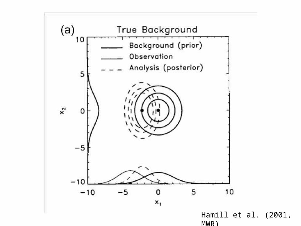
Hamill et al. (2001, MWR)

Hamill et al. (2001, MWR)