MPO 674 Lecture 15

3/3/15

Bayesian update

Jeff Anderson’s Tutorial• A | C = Prior based on previous information C• A | BC = Posterior based on previous

information C and new information B• B = New observational information

A | BC B | AC A | CPosterior Observation Prior

B

A | C A | BC

Courtesy Tom Hamill (NOAA/ESRL)

Forecast Model Cycle

MODEL “FIRST GUESS”

OBSERVATION PREPARATION

DATA ASSIMILATION

INITIAL CONDITIONS00 UTC

MODEL “FIRST GUESS”

OBSERVATION PREPARATION

DATA ASSIMILATION

INITIAL CONDITIONS06 UTC

MODEL “FIRST GUESS”

OBSERVATION PREPARATION

DATA ASSIMILATION

INITIAL CONDITIONS12 UTC

MODEL “FIRST GUESS”

OBSERVATION PREPARATION

DATA ASSIMILATION

INITIAL CONDITIONS18 UTC

Integrate 6 hours

Integrate 6 hours

Integrate 6 hours

Integrate 6 hours

FORECAST

Locations of meteorological stations from which Richardson obtained upper-air observations for his first numerical weather prediction. Squares marked 'P' provided atmospheric pressure values; those marked 'M' gave atmospheric momentum.

“Perhaps some day in the dim future it will be possible to advance the computations faster than the weather advances and at a cost less than the saving to mankind due to the information gained. But that is a dream.” L. F. Richardson

Subjective Analysis Objective Analysis

700 hPa Z

Gilchrist and Cressman (1954)

Successive Corrections: Cressman Analysis

Cressman Analysis

Three kinds of observation handled by the Cressman successive corrections scheme: height only, wind only, and height and wind together. R is the scan radius and d is the distance from the gridpoint at the center of the circle to the observation: height alone (i index), wind only (j index), height and wind (k index). The radius of influence is R; its value decreases on successive scans.

Cressman Analysis

• Advantages– Simple and computationally fast– Uses forecast information in background field

• Disadvantages– Does not include observation errors (bad obs?)– Does not account for distribution of observations– Level of detail depends on observation density– How to analyze wind versus height?– Does not account for background error

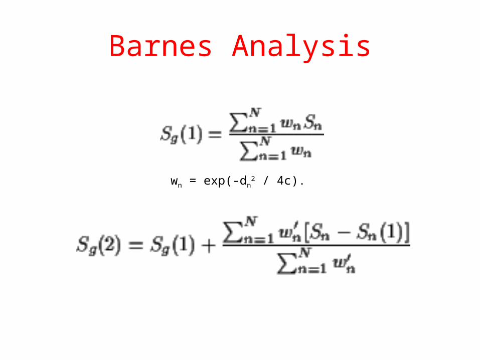
Barnes Analysis

wn = exp(-dn2 / 4c).

Barnes Analysis

• Advantages– No need for a model– No need to set influence radius– Control of fine-scale analysis

• Disadvantages– Same as for Cressman analysis

Nudging• Adds a “nudging” term to the prognostic equations

for the field variables.

• Initialize with first guess (background field) and integrate forward.

• Nudging term forces integration towards observations.

• Balanced initial conditions.• Good for small-scale obs (e.g. radar).• No covariance matrices.