Dynamic Assessment of Bridge Deck Performance Considering Realistic Bridge-Traffic Interaction

MPC 17-333 | Y. Zhou and S. Chen

Colorado State University North Dakota State University South Dakota State University

University of Colorado Denver University of Denver University of Utah

Utah State UniversityUniversity of Wyoming

A University Transportation Center sponsored by the U.S. Department of Transportation serving theMountain-Plains Region. Consortium members:

Dynamic Assessment of Bridge Deck Performance Considering Realistic Bridge-Traffic Interaction

Yufen Zhou

Suren Chen

Department of Civil and Environmental Engineering

Colorado State University

Fort Collins, Colorado

September 2017

Acknowledgements

The funds for this study were provided by the United States Department of Transportation to the

Mountain-Plains Consortium (MPC).

Disclaimer

The contents of this report reflect the views of the authors, who are responsible for the facts and the

accuracy of the information presented herein. This document is disseminated in the interest of information

exchange. The report is funded, partially or entirely, by a grant from the U.S. Department of

Transportation’s University Transportation Centers Program. However, the U.S. Government assumes no

liability for the contents or use thereof.

NDSU does not discriminate in its programs and activities on the basis of age, color, gender expression/identity, genetic information, marital status, national origin, participation in lawful off-campus activity, physical or mental disability, pregnancy, public assistance status, race, religion, sex, sexual orientation, spousal relationship to current employee, or veteran status, as applicable. Direct inquiries to Vice Provost for Title IX/ADA Coordinator, Old Main 201, NDSU Main Campus, 701-231-7708, ndsu.eoaa.@ndsu.edu.

ABSTRACT

Concrete bridge decks are directly exposed to daily traffic loads and may experience some surface

cracking caused by excessive stress or fatigue accumulation, which requires repair or replacement.

Among typical bridges in North America, bridge decks are considered the most expensive component to

construct and repair, not only because of direct repair cost repair, but also due to the indirect cost from the

traffic disruption during the repair action. In order to rationally predict the bridge deck response and the

damage risk, some appropriate analytical tools are needed to consider the dynamic effects between the

bridge and multiple vehicles moving in a realistic way. Such an analytical tool should be able to provide

rational prediction of the bridge global and local responses, such as displacement and stress on bridge

decks in addition to other members, which can be used for fatigue or other damage assessment. In the

present study, a hybrid dynamic analytical approach is developed for a typical multi-span concrete bridge

and stochastic traffic flow by considering the excitation from road roughness. Based on the dynamic

response results, the fatigue assessment is conducted with a focus on providing insights on vulnerable

locations and the impacts from varied traffic and road roughness conditions.

TABLE OF CONTENTS

1. INTRODUCTION AND LITERATURE REVIEW ......................................................................... 1

1.1 Background .................................................................................................................................... 1

1.2 Literature Review ........................................................................................................................... 1

1.2.1 Bridge-Vehicle Dynamic Interaction Analysis ................................................................. 1

1.2.2 Bridge-Traffic Dynamic Interaction Analysis .................................................................. 1

1.3 Organization of this Report ............................................................................................................ 2

2. HYBRID BRIDGE DYNAMIC MODEL .......................................................................................... 3

2.1 Refined-Scale Bridge Finite Element Model Using SAP2000 ....................................................... 3

2.2 Dynamic Vehicle Model ................................................................................................................ 3

2.2.1 Stochastic Traffic Flow Simulation .................................................................................. 3

2.2.2 Numerical Vehicle Model ................................................................................................. 4

2.3 Bridge-Vehicle Interaction Analysis .............................................................................................. 6

2.3.1 Reduced-DOF Bridge Model Based on Modal Coordinates ............................................. 6

2.3.2 Formulation of Bridge-Vehicle Interaction Analysis ........................................................ 6

2.3.3 Modeling of Road Surface Roughness with Progressive Deterioration ............................ 7

2.4 Response of Bridge Deck Through the Classic Plate Bending Theory ......................................... 8

2.5 Equivalent Moving Traffic Load (EMTL) ..................................................................................... 8

2.6 Fatigue Evaluation of Reinforced Concrete (RC) Decks ............................................................... 9

2.6.1 Punching Shear Strength and Fatigue Punching Shear Strength ....................................... 9

2.6.2 S-N Relations .................................................................................................................. 10

2.6.3 Equivalent Load Cycle Number Neq and the Fatigue Life .............................................. 10

3. NUMERICAL ANALYSIS ON PROROTYPE BRIDGE UNDER TYPICAL TRAFFIC

CONDITIONS .................................................................................................................................... 12

3.1 The Prototype Highway Bridge .................................................................................................... 12

3.1.1 Bridge Information .......................................................................................................... 12

3.1.2 Quantification of Punching Shear and Fatigue Punching Shear Strength of

the Prototype Bridge Deck ............................................................................................. 13

3.1.3 Development of Bridge Finite Element Model and Modal Properties ............................ 14

3.2 Stochastic Traffic Flow Simulation .............................................................................................. 16

3.3 Simulation of Road Surface Roughness ....................................................................................... 18

3.4 Displacement Response at the Bridge Deck ................................................................................. 18

3.5 Stress Response on the Bridge Deck ............................................................................................ 22

3.6 Equivalent Moving Traffic Load (EMTL) ................................................................................... 27

3.7 Fatigue Damage Prediction on the Bridge Deck .......................................................................... 28

4. PARAMETRIC STUDY OF BRIDGE-TRAFFIC INTERACTION AND FATIGUE

ANALYSIS ON BRIDGE DECK...................................................................................................... 30

4.1 Influence of Road Surface Roughness on the Bridge Deck ......................................................... 30

4.2 Influence of Traffic Flow Density ................................................................................................ 31

4.3 Influence of Vehicle Composition on the Traffic Flow ............................................................... 32

4.3 Fatigue Analysis ........................................................................................................................... 34

5. CONCLUSION ................................................................................................................................... 37

6. REFERENCES ................................................................................................................................... 38

LIST OF TABLES

Table 3.1 Modal frequencies, periods, and participation factors of the prototype bridge .................... 16

Table 4.1 Extreme absolute value of displacement and stress response under different road

conditions ............................................................................................................................. 31

Table 4.2 Extreme EMTL values over the bridge deck (unit: N) ......................................................... 35

Table 4.3 Maximum fatigue damage factors in one hour over the bridge deck (unit: N) .................... 36

LIST OF FIGURES

Figure 2.1 The numerical dynamic model for the heavy truck with one trailer ...................................... 5

Figure 2.2 Logarithm plots of S-N relations from repeated load tests of reinforced concrete slabs

under moving wheel loads ................................................................................................... 10

Figure 3.1 Prototype bridge (a) Plan View, (b) Elevation view of Bridge ............................................ 12

Figure 3.2a Finite element model of the prototype bridge ...................................................................... 14

Figure 3.2b Mode shapes of the first 10 modes of the prototype bridge ................................................. 15

Figure 3.3 Location of traffic lanes on the prototype bridge ................................................................. 16

Figure 3.4 Simulated busy traffic flow in the three lanes ...................................................................... 17

Figure 3.5 Simulated road surface roughness profile ............................................................................ 18

Figure 3.6 Node numbers in the bridge deck joints of the bridge model .............................................. 18

Figure 3.7 Element numbers in the bridge deck of the bridge model .................................................... 19

Figure 3.8 Wheel location of each type of vehicle on each lane ........................................................... 19

Figure 3.9 Locations of representative nodes in each span ................................................................... 19

Figure 3.10 Vertical displacement response at representative nodes on the bridge deck ........................ 20

Figure 3.11 Lateral displacement response at representative nodes on the bridge deck ......................... 20

Figure 3.12 Torsional displacement response at representative nodes on the bridge deck ..................... 20

Figure 3.13 Filled contour plot of the extreme vertical displacement all over the deck ......................... 21

Figure 3.14 Filled contour plot of the extreme torsional displacement all over the deck........................ 21

Figure 3.15 Locations of representative elements in each span .............................................................. 22

Figure 3.16 Normal stress (σxx) of the top surface of representative elements on the bridge deck.......... 22

Figure 3.17 Normal stress (σyy) of the top surface of representative elements on the bridge deck.......... 22

Figure 3.18 Shear stress (σxy) of the top surface of representative elements on the bridge deck ............. 23

Figure 3.19 Extreme negative normal stress (σxx) of the top surface on the bridge deck ........................ 23

Figure 3.20 Extreme negative normal stress (σyy) of the top surface on the bridge deck ........................ 24

Figure 3.21 Extreme negative shear stress (σxy) of the top surface on the bridge deck ........................... 24

Figure 3.22 Normal stress (σxx) of the bottom surface of representative elements on the bridge deck ... 25

Figure 3.23 Normal stress (σyy) of the bottom surface of representative elements on the bridge deck ... 25

Figure 3.24 Shear stress (σxy) of the bottom surface of representative elements on the bridge deck ...... 25

Figure 3.25 Extreme positive normal stress (σxx) of the bottom surface on the bridge deck ................... 26

Figure 3.26 Extreme positive normal stress (σyy) of the bottom surface on the bridge deck ................... 26

Figure 3.27 Extreme positive shear stress (σxy) of the bottom surface on the bridge deck ...................... 27

Figure 3.28 Time histories of vertical EMTL at representative nodes on the bridge deck...................... 27

Figure 3.29 Filled contour plot of the extreme value of vertical EMTL over the bridge deck ................ 28

Figure 3.30 Fatigue damage factor in one hour over the bridge deck ..................................................... 29

Figure 3.31 Common logarithm of fatigue damage factor in one hour over the bridge deck ................. 29

Figure 4.1 Vertical displacement time histories at Node 1102 for different road surface conditions ... 30

Figure 4.2 Torsional displacement time histories at Node 1102 for different road surface conditions . 30

Figure 4.3 Normal stress time history (σxx) at the bottom surface of Element 1087 for different road

surface conditions ................................................................................................................ 31

Figure 4.4 Shear stress time history (σxy) at the bottom surface of Element 1087 for different road

surface conditions ................................................................................................................ 31

Figure 4.5 Vertical displacement history at the representative node (#1102) on the bridge deck

under traffic flow with different densities ............................................................................ 32

Figure 4.6 Normal stress history at the representative element (#1087) on the bridge deck under

traffic flow with different densities ...................................................................................... 32

Figure 4.7 Vertical displacement histories at the representative node (#1102) on the bridge deck

under traffic flow with different vehicle proportions ........................................................... 33

Figure 4.8 Torsional displacement histories at the representative node (#1102) on the bridge deck

under traffic flow with different vehicle proportions ........................................................... 33

Figure 4.9 Normal stress histories (σxx) at the representative element (#1087) on the bridge deck

under traffic flow with different vehicle proportions ........................................................... 33

Figure 4.10 Shear stress histories (σxy) at the representative element (#1087) on the bridge deck

under traffic flow with different vehicle proportions ........................................................... 34

Figure 4.11 Extreme EMTL over the bridge deck under different road roughness conditions and

vehicle proportions ............................................................................................................... 35

Figure 4.12 The maximum fatigue damage factor in one hour over the bridge deck under different

road roughness conditions and vehicle proportions ............................................................. 36

1

1. INTRODUCTION AND LITERATURE REVIEW

1.1 Background

Highway bridges support increasing daily traffic due to the growth of social, economic, and recreational

needs in the community. In the United States, there are about 583,000 bridges around the nation, 235,000

of which are made of conventional reinforced concrete (Koch et al. 2002). Concrete bridge decks are

directly exposed to daily traffic loads and may experience some surface cracking caused by excessive

stress or fatigue accumulation, which requires repair or replacement. In fact, among typical bridges in

North America, bridge decks are considered the most expensive component to construct and repair

(Lounis 2003) because of the direct cost of repair, as well as the indirect cost from the traffic disruption

during the repair action (Oh 2007). In order to rationally predict the bridge deck response, an appropriate

analytical tool is needed to consider the dynamic coupling between the bridge and multiple vehicles

moving in a realistic way. Such an analytical tool should be able to provide rational prediction of the

bridge’s global and local responses, such as displacement and stress on bridge decks, which can be used

for fatigue or other damage assessment. In the present study, a new dynamic analytical approach is

developed for a typical multi-span concrete bridge and stochastic traffic system by considering the

excitations from road roughness. Based on the dynamic response results, the fatigue assessment is also

conducted focusing on providing some insights on vulnerable locations and the impacts from different

traffic and road roughness conditions.

1.2 Literature Review 1.2.1 Bridge-Vehicle Dynamic Interaction Analysis

The studies on the dynamic effects from vehicles date back to the 1970s. The investigation of bridge

vibrations under moving vehicle loads has been traditionally conducted by treating a vehicle as a moving

load (Olsson 1991), a moving mass (Lee 1996), or a moving spring mass (Yang and Wu 2001). It has

long been observed that when a bridge is subjected to moving vehicle loads, the induced dynamic

deflections and stresses can be significantly higher than those only considering the static load effects of

vehicles (Yang and Yau 1997). The dynamic interaction between passing vehicles and the bridge may be

even more significant when increasing traffic volume is involved. The bridge and moving vehicles are

interacting as coupled dynamic systems, especially when vehicles are moving. On one hand, vibrating

heavy road vehicles may significantly change local and global dynamic behavior and affect the fatigue

life of the bridge. On the other hand, the vibration of the bridge may in turn affect the dynamic

performance of the vehicles, which may pose significant influence on vehicle safety and comfort of the

drivers and passengers.

1.2.2 Bridge-Traffic Dynamic Interaction Analysis Most of the existing studies dealt with the interactions between bridge and a single vehicle or a series of

vehicles at certain intervals driven through the bridge at constant speeds (Cai and Chen 2004; Guo and Xu

2006). Nevertheless, considering that traffic on the bridge is stochastic following certain rules, e.g.,

accelerating, decelerating, and braking, the interactions between the bridge and vehicles may be largely

different from those with a series of vehicles driven at equal intervals with constant speeds. For short- or

medium-span bridges, although the total number of vehicles on the bridge is limited, more realistic

information of individual vehicles, such as instantaneous locations and speeds, are also critical to both

predicting global bridge response and assessing possible local damage, such as on the bridge deck.

Comparatively, the information obtained from the assumed traffic patterns (i.e., one vehicle or equal

2

intervals) is apparently not realistic and may provide inaccurate predictions of the bridge performance,

such as global response and local cracking and fatigue damage on the bridge deck or other members.

Chen and Wu (2010) proposed a simulation approach to evaluate the long-span bridge dynamic

performance considering the combined effects of wind and stochastic traffic (Chen and Wu 2011). The

approach approximately replaced each individual vehicle dynamic model with the equivalent dynamic

wheel loading (EDWL) obtained from the bridge-single-vehicle interaction analysis (Chen and Cai 2007).

Such an approach (Chen and Wu 2010), however, did not couple all the vehicles and the bridge

simultaneously, and therefore the dynamic interaction effects from multiple vehicles cannot be fully taken

into account in the analysis. In addition, the dynamic performance of each individual vehicle in the

stochastic traffic flow cannot be rationally obtained even though the bridge response can be reasonably

approximated under dynamic excitations from stochastic traffic. Recently, Zhou and Chen (2015)

developed a fully-coupled analytical platform of the long-span bridge/traffic system, which can couple

each individual vehicle and the bridge under different dynamic loads for the first time. However, this

approach cannot be directly applied to short- and medium-span bridges to investigate the bridge deck

performance. This is primarily due to different formulations for short- and medium-span girder bridges as

compared with typical box girders of long-span bridges, and also most existing studies on long-span

bridges (e.g., Zhou and Chen 2015) do not include refined modeling of bridge decks essential to

providing detailed response information of the deck.

This study will present a hybrid analytical approach to assess the dynamic performance of bridge decks

on typical multi-span highway bridges under normal stochastic traffic flow. The hybrid bridge dynamic

model is composed of a refined finite element model of the bridge and a fully-coupled bridge-traffic

interaction model using modal coordinates. Taking advantage of the strength of commercial software for

detailed bridge deck modeling and a mode-based bridge-traffic model for coupled interaction effects, the

proposed analytical approach is able to directly consider dynamic interactions of the bridge and multiple

vehicles in the traffic flow. In addition, the detailed dynamic responses of the bridge deck in terms of

strain, stress, and internal force can be obtained from the primary response of the simulation model

through the finite element shape functions. Fatigue assessment on the bridge deck is also conducted by

quantifying the fatigue factor within one hour under several representative traffic conditions. The spatial

distribution of the fatigue factor over the bridge deck is studied under different traffic, road roughness,

and vehicle composition conditions. Finally, a parametric study is conducted in terms of the impacts of

road roughness, traffic densities, and vehicle compositions.

1.3 Organization of this Report

The report is composed of five sections.

Section 1 introduces pertinent background information and literature review results related to the present

study. In Section 2, the hybrid bridge dynamic model is developed. In Section 3, a prototype bridge is

studied with the developed model to investigate the bridge response of typical multi-span concrete

bridges. In Section 4, parametric studies are conducted to study the effects of several parameters. The

report concludes with Section 5.

3

2. HYBRID BRIDGE DYNAMIC MODEL

The formulation of bridge-vehicle interaction model is dependent on the instantaneous response of the

bridge and each individual vehicle. Therefore, the dynamic analysis needs to proceed iteratively at each

time step, which presents a challenge for common commercial finite element programs since the built-in

modules of most software are usually difficult to incorporate into iterative analysis functions. However,

commercial finite element programs have advantages in sophisticated finite element formulations,

nonlinear effect considerations, and advanced meshing options, which make them good candidates for

detailed modeling of a bridge deck on a multi-span highway bridge. The hybrid bridge dynamic model

combines the finite element bridge model and the mode-based bridge-traffic interaction model. In the

mode-based bridge-traffic interaction model, the bridge is modeled using modal coordinates and the

vehicles are modeled using physical coordinates. The bridge displacement response can be obtained

through the analysis as the primary bridge responses. The dynamic displacement response of each

individual vehicle can also be obtained from the simulation analysis. By adopting plate-bending theory,

the detailed bridge deck response, including strain, stress, and internal forces, can be obtained through

applying the finite element shape functions.

2.1 Refined-Scale Bridge Finite Element Model Using SAP2000

To accurately represent the 3-D bridge behavior, a bridge deck can be traditionally modeled using a plate

model or a grillage model. Plate bridge models have been used to investigate the bridge dynamic

performance under moving vehicles, as demonstrated in several studies (Olsson 1985; Zhu and Law 2002;

González et al. 2010). Alternatively, grillage bridge models are also found in the literature for bridge

dynamic analyses considering the interactions with moving vehicles, as seen in the references (Huang et

al. 1992; Nassif and Liu 2004). In the grillage bridge model, the bridge deck is discretized as skeletal

structure consisting of a mesh of 1-D beam elements. Although grillage modeling of a bridge deck has

some advantages in simplicity and computational efficiency, it is an approximate model for the bridge

deck performance prediction. For instance, the internal force is discontinuous at the grillage nodes for a

normal mesh and, as a result, the stress distributions on the bridge deck cannot be realistically obtained. In

the present study, a plate element is adopted for bridge deck modeling of the multi-girder highway bridge.

Commercial finite element software SAP2000 is a popular finite element modeling and analysis tool

widely adopted in the design practices and some research works of bridge and building structures.

SAP2000 is adopted in the study to develop the refined-scale bridge finite element model.

2.2 Dynamic Vehicle Model

2.2.1 Stochastic Traffic Flow Simulation

In this study, the three-lane cellular automaton model is adopted to simulate the instantaneous behavior of

vehicles both temporally and spatially. As a mathematical idealization of physical systems with discrete

time and space, cellular automaton consists of a finite set of discrete variables to represent specific

vehicle information. The discrete variables for any individual vehicle include the occupied lane,

longitudinal location, type, speed, and driving direction. The variables in each cell are updated based on

the adjacent vehicle information and the probabilistic traffic rules regulating accelerating, decelerating,

lane changing, and braking. Detailed traffic rules involved in the traffic flow simulation are referred to

the published paper of Chen and Wu (2010). The cellular automaton-based traffic flow simulation is

performed on a roadway-bridge-roadway system to simulate the stochastic traffic flow through the bridge

in a realistic way. The randomization of the traffic flow is realized by the stochastic initial variables in the

cellular of the entire system. Periodic boundary conditions are adopted in the traffic flow model, in which

the total number of each type of vehicle in the system remains constant. The vehicles in the simulated

4

traffic flow are classified into three types: heavy multi-axle truck, light truck, and sedan. The vehicle

classification ratios defining the composition of different types of vehicles in the traffic flow are usually

quantified based on the site-specific traffic data or generic traffic statistics when the specific data are not

available.

2.2.2 Numerical Vehicle Model

The vehicles in the stochastic traffic are categorized into three types from a variety of vehicle

configurations: heavy truck with one trailer, light truck, and light car. The vehicles are modeled as a

combination of several rigid bodies, wheel axles, springs, and dampers. The main rigid bodies are

modeled to represent the vehicle bodies. The suspension system of each axle is modeled as the upper

springs and the elastic tires are modeled as lower springs. Viscous dampers are adopted to model the

energy dissipation system. The mass of the suspension system is assumed to be concentrated on each

wheel axle while the mass of the springs and dampers are assumed to be zero. Four degrees of freedom

are associated with the main rigid body, including the two translational and two rotational degrees of

freedom. The constraint equations are applied in deriving the vehicle matrices for the heavy truck model

in which a pivot is used to connect the truck tractor and the trailer. The numerical dynamic model for the

heavy truck contains two main rigid bodies, three-wheel axle sets, 24 sets of springs, and dampers in

either vertical or lateral direction, shown in Figure 2.1. The displacement vector 𝑑𝑣 for the heavy truck

model contains 19 degrees of freedom, including eight independent vertical, eight lateral and three

rotational degrees of freedom, which is demonstrated in Eq. (1).

}{ 3322112133221122111 RaLaRaLaRaLarrRaLaRaLaRaLarrrrrv YYYYYYYYZZZZZZZZd (1)

in which, 𝑍𝑟𝑖 represents the vertical displacement of the ith rigid body; 𝜃𝑟𝑖 represents the rotational

displacement of the ith rigid body in the x-z plane; 𝛽𝑟𝑖 represents the rotational displacement of the ith

rigid body in the y-z plane; 𝑍𝑎𝑖𝐿(𝑅) represents the vertical displacement of the ith wheel axle in the left

(right) side; 𝑌𝑟𝑖 represents the lateral displacement of the ith rigid body; 𝑌𝑎𝑖𝐿(𝑅) represents the lateral

displacement of the ith wheel axle in the left (right) side.

5

(a) Elevation view

(b) Side view

Figure 2.1 The numerical dynamic model for the heavy truck with one trailer

The springs and dampers are labeled according to the related axle number, upper-lower orientation, y-z

direction, and left-right location, which are corresponding to the superscript and three subscripts,

respectively, in the notation of each stiffness coefficient 𝐾 or damping coefficient 𝐶. The numerical

dynamic model for the light truck consists of one main rigid body, two-wheel axle sets, and 16 sets of

springs and dampers vertically or laterally. The side view of the numerical model for the light truck and

bus is the same as shown in Figure 2.1 (b) and hereby not shown for brevity. The displacement vector 𝑑𝑣

for the light truck consists of 12 degrees of freedom, including five independent vertical, five lateral and

two rotational degrees of freedom, as demonstrated in Eq. (2).

}{ 221112211111 RaLaRaLarRaLaRaLarrrv YYYYYZZZZZd (2)

The numerical model for the light car is similar to the model for light truck except that the vehicle

dimensions and mass properties require different parameter inputs. The input data for the vehicle models

include the mass and mass moment inertia of each rigid body, the mass of each wheel axle set, the

stiffness coefficient of each spring, the damping coefficient of each damper, and the vehicle dimensions.

6

2.3 Bridge-Vehicle Interaction Analysis

2.3.1 Reduced-DOF Bridge Model Based on Modal Coordinates

Like most commercial software, SAP2000 cannot directly couple moving vehicle models to conduct the

dynamic interaction analysis of the bridge and moving vehicles subject to various roughness excitations.

The most applicable approach is to generate equivalent nodal time-history excitation inputs of wheel

loadings from passing vehicles. The multi-mode, reduced-order bridge dynamic model has been used

widely in the bridge dynamic analysis under wind, seismic, or other dynamic loads such as vehicles. After

the detailed FEM model of the bridge is developed, modal analysis is conducted to extract the first couple

critical modes to the bridge dynamic response. With the selected critical modes, a reduced-DOF bridge

dynamic model is developed to capture the dynamic response of the entire bridge with reasonable

accuracy by adopting only limited modes (Guo and Xu 2003; Chen and Cai 2007).

2.3.2 Formulation of Bridge-Vehicle Interaction Analysis

Based on the reduced-order bridge model, the coupled dynamic interaction model of a typical bridge and

any number of moving vehicles subjected to road roughness profile excitations can be developed (Zhou and

Chen 2015).

r

v

r

v

r

b

n

i

G

v

v

v

b

vbv

vbv

vbvb

n

i bcib

v

v

b

vbv

vbv

vbvb

n

i bcib

v

v

b

v

v

b

nnnn

n

nnn

n

nn

F

F

FF

U

U

U

KK

KK

KKKK

U

U

U

CC

CC

CCCC

U

U

U

M

M

M

1

1

111

1

111

1

11

1

,

,

,,1

,

,

,,1

0

0

00

00

00

000

000

000

000

(3)

in which Mb, Kb, and Cb are the generalized mass, stiffness, and damping matrices for the bridge structure,

respectively; n is the number of vehicles traveling on the roadway-bridge-roadway system in the traffic

flow; Mv, Kv, and Cv are the mass, stiffness, and damping matrices of the ith vehicle in the traffic flow,

respectively; Kbci and Cbci refer to the stiffness and damping contribution to the bridge structure due to the

coupling effects between the ith vehicle in the traffic flow and the bridge system, respectively; ivbK , and

ivbC ,

are the coupled stiffness and damping matrices contributing to bridge vibration from the ith vehicle in the

traffic flow, respectively; bviK , and bvi

C , are the coupled stiffness and damping matrices contributing to the

vibration of the ith vehicle in the traffic flow from the bridge structure; Ub is a vector of generalized

coordinates of the bridge corresponding to each mode involved in the analysis; ivU is a vector of the

physical responses corresponding to each degree of freedom of the ith vehicle in the traffic flow; one-dot

and two-dot superscripts of the displacement vector denote the velocity and acceleration, respectively; Fb

and ivF denote the externally applied loads for the bridge in modal coordinates and the ith vehicle in

physical coordinates, respectively. The superscripts r and G denote the loads due to road roughness and

self-weight, respectively.

7

2.3.3 Modeling of Road Surface Roughness with Progressive Deterioration

The road surface roughness on the approaching road and the bridge deck is modeled as a stationary

Gaussian random process with zero mean value. The road surface roughness r can be generated by the

spectral representation formulation, which was first introduced by Shinozuka and Jan (1972) and

expressed in Eq. (4).

)2cos()(2)(1

kk

n

ik xSxr

(4)

in which n is the number of points in the inverse Fourier Transform; x is the location on the road surface;

θk is the random phase angle with a uniform distribution between 0 and 2 ; ϕ is the power spectral

density function, which adopts the formation suggested by Huang and Wang (1992).

2

0

0 ))(()( n

nnn (5)

in which n is the spatial frequency (cycle/m); n0 is the discontinuity frequency of 1/2π (cycle/m); )( 0n is

the road roughness coefficient (m3/cycle).

The road roughness coefficient is predicted using the international roughness index (IRI) (Shiyab 2007).

6)42808.0/(9

0 102101972.6)( IRIen (6a)

The IRI values at time t can be calculated using the following equation (Paterson 1986),

t

t CESALSNCIRIeIRI )()1(26304.1 5

0

(6b)

in which 0IRI is the initial roughness value; t is time in years; η is the environmental coefficient; SNC is

the structural number; (CESAL)t is the estimated number of traffic at time t in millions.

The road roughness coefficient in a 15-year period can be calculated as follows (Dodds 1972).

yearstwhenconditionpoor

yearstwhenconditionaverage

yearstwhenconditiongood

yearstwhenconditiongoodvery

n

151410320

131080

12111020

10105

)(

6

6

6

6

0 (7)

8

2.4 Response of Bridge Deck Through the Classic Plate Bending Theory The strain vector is composed of normal strains in x and y directions and shear strains. The linear bending

strain is caused by the vertical displacement of the plate and expressed in the following equation,

242

221

22 4

2 21

2 24

1

{ }

2

2 2

ii

i

xx xx

iyy yy i

i

xy xy

ii

i

ww

xx

wz z w

y y

ww

x y x y

(8)

in which w is the vertical displacement; z is the vertical distance from the center line to the plate surface.

The stress vector can be obtained from the strain vector and expressed as follows:

2 2

2 2

01 1

{ } 01 1

2 0 0

xx xx xx

yy yy yy

xy xy xy

EE

E E

G

(9)

in which E is elastic modulus, Υ is the Poisson’s ratio.

2.5 Equivalent Moving Traffic Load (EMTL)

The equivalent wheel loads (EWL) can be obtained directly for each vehicle in the stochastic traffic flow

from the time-history simulation results of the fully-coupled bridge-traffic interaction system. The vertical

equivalent moving traffic loads (EMTL) for the bridge girder joints are further accumulated by

distributing the EWL for each vehicle linearly to the bridge deck joints both longitudinally and laterally.

The EWL for the ith vehicle is determined as the summation of the vertical equivalent dynamic wheel

loads and the gravity loads as expressed in Eq. (10).

iiz

edwl

iz

ewl GtFtF )()( (10)

in which iG is the gravity load of the ith vehicle; )(tF iz

edwl is the vertical dynamic wheel loads for the ith

vehicle in the traffic flow at time instant t , which are defined as (Chen and Cai 2007):

na

jajR

j

lzRajR

j

lzRajL

j

lzLajL

j

lzL

iz

edwl tZCtZKtZCtZKtF1

))(ˆ)(ˆ)(ˆ)(ˆ()(

(11)

in which )(ˆ)( tZ RajL

and )(ˆ)( tZ RajL

are the relative vertical displacements and the corresponding first

derivatives between the lower mass block on the vehicle at the left (right) side and the contacting point on

the bridge, respectively; na is the total number of wheel axles for the ith vehicle; K and C are the stiffness

and damping coefficients of the springs and dampers in the vehicle model, respectively; the subscripts l, z,

9

L(R) represent lower position, vertical (z) direction, and left (right) side for the springs or dampers,

respectively.

The corresponding vertical equivalent wheel loads for the ith vehicle in the pth modal coordinate of the

bridge subsystem can be expressed in the following equation,

na

j

pi

j

i

jR

pi

j

i

jajR

j

lzRajR

j

lzR

na

j

pi

j

i

jL

pi

j

i

jajL

j

lzLajL

j

lzL

piz

ewl

ttdthGtZCtZK

ttdthGtZCtZKtF

1

1

))()()()()(ˆ)(ˆ(

))()()()()(ˆ)(ˆ()(

(12)

in which i

jG is the gravity load at the jth axle of the ith vehicle; )(th pi

j and )(tpi

j are pth modal coordinates

in the vertical and rotational directions for the jth axle of the ith vehicle at time instant t, respectively;

)(td i

jL and )(td i

jR are the transverse distances to the centerline for the jth axle of the ith vehicle at the left

and right sides, respectively.

2.6 Fatigue Evaluation of Reinforced Concrete (RC) Decks

2.6.1 Punching Shear Strength and Fatigue Punching Shear Strength The punching shear strength of the RC bridge deck can be obtained from the stress distributions when the

bridge deck experiences shear failure. A shear failure model developed by Matsui (1984) is adopted to

evaluate the punching shear strength of the RC bridge deck.

In the punching shear failure model (Matsui 1984), punching shear strength psV of the bridge deck is

expressed as:

]22242[]2222[ maxmax dmmddtmddmsps CdaCbdCxxbxxaV (13a)

Fatigue punching shear strength 0fP is defined as:

mtmsf CxBP maxmax0 2 (13b)

where maxs is the maximum shear strength of concrete and

maxt is the maximum tensile strength of

concrete:

''

max 00251.0252.0 ccs ff (13c)

3/2'

max 269.0 ct f (13d)

'

cf is compressive strength; a is the length of loaded area in bridge transverse direction; b is the length of

loaded area in bridge longitudinal direction; mx and

dx are neutral axis depths measured from the top

surface of the bridge deck in the bridge transverse and longitudinal direction, respectively; md and

dd are

effective depths of longitudinal and transverse bars, respectively; mC and

dC are concrete covers of

transverse and longitudinal bars, respectively; B is the effective width and ddbB 2 .

10

2.6.2 S-N Relations

The S-N relations of reinforced concrete decks are developed by Matsui (1984) through repeated load

tests. In the study by Matsui (1984), a series of dry and wet reinforced concrete slabs are tested under

moving wheel loads to determine the relations between load level S and cycles-to-fatigue N. The test

results are demonstrated in Figure 2.2.

Figure 2.2 Logarithm plots of S-N relations from repeated load tests of reinforced concrete slabs under

moving wheel loads (Matsui 1984)

The S-N relation for dry RC slab

21 logloglog CNCS (14a)

in which 0/ fa PPS ; Pa is the applied shear load; Pf0 is the fatigue punching shear strength; 0784.01 C ;

52.12 C .

The cycles-to-fatigue can be expressed as

)log(log/1 2110SCC

N

or 1/1

2

C

S

CN

(14b-c)

2.6.3 Equivalent Load Cycle Number Neq and the Fatigue Life

According to the S-N curves for the bridge concrete deck under vehicle wheel loads, the bridge deck fails

at different numbers of load cycles under different applied shear loads. Suppose that the bridge deck fails

at N1 and N2 load cycles under applied shear load P1 and P2, respectively. The following relations can be

obtained:

21101 loglog)/log( CNCPP f (15a)

22102 loglog)/log( CNCPP f (15b)

which will give,

21011/ CNPP

C

f (15c)

11

22021/ CNPP

C

f (15d)

By dividing the equations on the left and right hand side, the fatigue shear strength 0fP will be eliminated

and the relation between numbers of load cycles N1 and N2 can be obtained.

2

/1

1

21

1

NP

PN

C

(16)

The fatigue damage is assumed to be accumulated in a linear mechanism, and Miner’s rule is applied to

calculate the equivalent number of load cycles Neq. Supposing the bridge deck fails at N0 cycles under

applied load P0, the equivalent number of load cycles Neq during certain time period t0 seconds

corresponding to the example applied load P0 can be expressed as (Oh et al. 2007),

i

Cn

i

iteq NPPN1

0

/1

1

0, /

(17)

in which Pi and Ni are the applied shear load and number of cycles at different load levels during time

period t0, respectively; n is the total number of load levels during time period t0.

Fatigue damage factor γ0 during one hour is obtained using the following equation:

00

,

0

60600

tN

N teq (18)

The bridge deck is considered to reach fatigue life if γ0 reaches 1.0. Supposing that the load cycles in the

certain time period t0 seconds can represent the typical load condition of the bridge deck in the lifetime,

the cumulative equivalent number of load cycles in a year will be

0,

0

,

606024365teqyeareq N

tN

(19)

The fatigue life of the bridge deck (year) is calculated by the following equation:

yeareqyear N

NLife

,

0 (20)

12

3. NUMERICAL ANALYSIS ON PROROTYPE BRIDGE UNDER TYPICAL TRAFFIC CONDITIONS

3.1 The Prototype Highway Bridge 3.1.1 Bridge Information

The multi-span highway bridge under investigation has three continuous spans in the longitudinal

direction with a span length of 22.1 m, 29.5 m, and 22.1 m, respectively. The bridge superstructure

(Figures 3.1a-b) is composed of an 8-in. concrete slab deck supported by eight parallel pre-stressed

concrete I-girders with a 5-ft., 8-in. depth (Figure 3.1b). The bridge girders are equally distributed in the

transverse direction with a girder spacing of 2.419 m. The girders are reinforced longitudinally at the tops

of the cross sections and are braced with stirrups at 18-in. intervals. The junctions between adjacent

girders, supported by the pier cap, are embedded in a concrete diaphragm creating an integral and fixed

connection. Supporting the concrete diaphragms are rectangular pier caps of 5-ft. depth, each supported

by interior and exterior columns with constant average depths (Figure 3.1b). Each column contains

standard longitudinal reinforcement, and transverse confinement at a 2-ft., 9-in. spacing. The integral

abutment is adopted for these bridges. So it encases the contiguous I-girders, and is also tied by

reinforcement to the adjacent deck.

(a) Plan View

13

Figure 3.1 Prototype bridge (a) Plan View, (b) Elevation view of Bridge (unit: m)

3.1.2 Quantification of Punching Shear and Fatigue Punching Shear Strength of the Prototype Bridge Deck Deck depth: h = 0.2032 m

Neutral axis x: ysyswc fAfAbxf '

1

' )(85.0

Concrete compressive strength: '

cf : PaEfc 74'

Rebar: ASTM 416 Grade 270

Rebar yield strength: PaEf y 9679.1

# 4 rebar diameter: 0.0127 m; area: 0.000129 m2

For the transverse bars in the main deck direction,

Neutral axis: mmE

E

bf

fAfAx

wc

ysys

m 02548.074*85.075.0

9679.1*000129.0*)0.36(

85.075.0 '

'

Loaded length in the transverse direction of the bridge (main direction of bridge deck): mincha 508.020

Concrete cover: mCm 05.0

Effective depth: mChd mm 1532.005.02032.0

For the longitudinal bars in the distribution deck direction,

Neutral axis: mmE

E

bf

fAfAx

wc

ysys

d 01699.07485.075.0

9679.1000129.0)0.24(

85.075.0 '

'

Loaded length in the direction of traffic (distribution direction of bridge deck) for HS20 in AASHTO:

minchb 2054.010

Concrete cover: mCd 0627.0

Effective depth: mChd dd 1405.0

Maximum shear strength of concrete: Paff ccs 998000000251.0252.0 ''

max

Maximum tensile strength of concrete: Pafct 31462269.03/2'

max

(b) Elevation View

14

Punching shear strength:

N

CdaCbdCxxbxxaV dmmddtmddmsps

254560

0.0627)0.1532)2+10(0.02542+0.05)100.0254+0.14052+0.0627(4(231462

0.02548)0.01699)2+10(0.02542+0.016990.02548)2+10(0.0254(29980000

]22242[]2222[ maxmax

Fatigue punching shear strength:

N

CxdbCxBP mtmsdmtmsf

273770

0.05)*31462+0.02548*(9980000*0.1405)*2+10*(0.0254*2

222 maxmaxmaxmax0

3.1.3 Development of Bridge Finite Element Model and Modal Properties

The plate element on the bridge deck has a rectangular shape with a length, width, and depth of 0.884 m,

0.914 m, and 0.205 m, respectively. The bridge deck is connected to bridge girders through rigid link

elements. The bridge finite element model in SAP2000 is shown in Figure 3.2a and the mode shapes of

the first ten modes are given in Figure 3.2b (a-j) (Wilson et al. 2014), and the modal properties are

summarized in Table 3.1.

Figure 3.2a Finite element model of the prototype bridge

(1) Mode 1 (1st longitudinal mode) (2) Mode 2 (1st vertical mode)

15

(3) Mode 3 (2nd vertical mode) (4) Mode 4 (3rd vertical mode)

(5) Mode 5 (4th vertical mode) (6) Mode 6 (5th vertical mode)

(7) Mode 7 (6th vertical mode) (8) Mode 8 (7th vertical mode)

(9) Mode 9 (8th vertical mode) (10) Mode 10 (9rd vertical mode)

Figure 3.2b Mode shapes of the first 10 modes of the prototype bridge (scale factor: 60)

16

Table 3.1 Modal frequencies, periods, and participation factors of the prototype bridge

Mode Frequency

(Hz)

Period

(Sec)

UX

(N-s2)

UY

(N-s2)

UZ

(N-s2)

RX

(N-m-s2)

RY

(N-m-s2)

RZ

(N-m-s2)

1 1.704 0.587 43981 0 0 -1 24047 -1

2 5.425 0.184 0 7 11111 10 -93 -36

3 5.637 0.177 0 -899 13 -66048 158 -28

4 6.513 0.154 0 -57 -420 216 343 354

5 7.584 0.132 -2 -37270 36 33991 1170 2704

6 8.175 0.122 -1 4309 14 -17730 558 -653

7 8.428 0.119 -1066 59 81 521 708241 -802

8 8.611 0.116 -9 -117 -160 -1578 5510 116728

9 9.024 0.111 2 88 35428 2733 -1241 595

10 9.118 0.110 2 4751 -439 192147 -304 1699

3.2 Stochastic Traffic Flow Simulation

The stochastic traffic flow is simulated on the three lanes in the same driving direction. The cell length in

the cellular automaton model is 7.5 m. The vehicles in the traffic flow are categorized as three types: light

car, light truck, and heavy truck. The vehicle percentages for light car, light truck, and heavy truck are

50%, 30%, and 20%, respectively. The stochastic traffic flow is simulated on a roadway-bridge-roadway

path in order to take into account the initial dynamic effects of the moving vehicles when they enter the

bridge. The roadway is assumed to be located at the two ends of the bridge with a length of 75 m each,

which is the same as the total bridge length. Busy traffic flow is assumed to be present on the bridge with

a vehicle density of 33 vehicles/km/lane. The maximum vehicle speed is 30 m/s, which is equal to four

times the cell length. The distribution of three through lanes and their locations on the bridge girders are

shown in Figure 3.3.

Figure 3.3. Location of traffic lanes on the prototype bridge (unit: m)

The simulated stochastic traffic flow is shown in Figures 3.4(a-c), respectively, for the fast lane, middle

lane, and slow lane.

17

(a) Traffic flow in the fast lane

(b) Traffic flow in the middle lane

(c) Traffic flow in the slow lane

Figure 3.4. Simulated busy traffic flow in the three lanes (· heavy truck; o light truck; + light car)

18

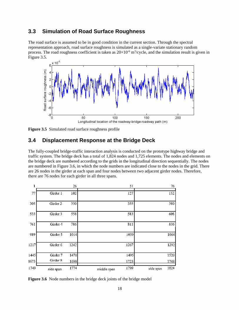
3.3 Simulation of Road Surface Roughness The road surface is assumed to be in good condition in the current section. Through the spectral

representation approach, road surface roughness is simulated as a single-variate stationary random

process. The road roughness coefficient is taken as 20×10-6 m3/cycle, and the simulation result is given in

Figure 3.5.

Figure 3.5 Simulated road surface roughness profile

3.4 Displacement Response at the Bridge Deck The fully-coupled bridge-traffic interaction analysis is conducted on the prototype highway bridge and

traffic system. The bridge deck has a total of 1,824 nodes and 1,725 elements. The nodes and elements on

the bridge deck are numbered according to the grids in the longitudinal direction sequentially. The nodes

are numbered in Figure 3.6, in which the node numbers are indicated close to the nodes in the grid. There

are 26 nodes in the girder at each span and four nodes between two adjacent girder nodes. Therefore,

there are 76 nodes for each girder in all three spans.

Figure 3.6 Node numbers in the bridge deck joints of the bridge model

19

The numbers of elements around the representative nodes are shown in Figure 3.7. It can be seen that for

the bridge deck section between two adjacent girders in each span is divided into 5×3 elements.

Figure 3.7 Element numbers in the bridge deck of the bridge model

According to the wheel locations of vehicles on the lanes in Figure 3.8, the representative deck nodes are

selected as node 1077, 1102, and 1127 in the left side span, middle span, and right side span, respectively.

The locations of the representative nodes are demonstrated in Figure 3.9 with more detailed nodes on the

deck.

Figure 3.8 Wheel location of each type of vehicle on each lane (unit: m)

Figure 3.9 Locations of representative nodes in each span

20

The time-history responses at three representative nodes of the bridge under the traffic are given in

Figures 3.10-12 for the vertical, lateral, and torsional displacements, respectively. For vertical and

torsional displacements, Node 1102, located in the middle of the main span, exhibits the largest response.

For lateral displacement, the responses at the three representative nodes are similar, with peak values at

different time.

Figure 3.10 Vertical displacement response at representative nodes on the bridge deck

Figure 3.11 Lateral displacement response at representative nodes on the bridge deck

Figure 3.12 Torsional displacement response at representative nodes on the bridge deck

21

By obtaining the extreme values of the time-history responses of all the nodes across the bridge deck, a

contour plot of the extreme values on the bridge deck is made for the vertical displacement (Figure 3.13)

and torsional displacement (Figure 3.14). As shown in Figure 3.13, the largest extreme vertical

displacement for each span happens in the middle span around the middle portion in the transverse

direction. Comparatively, the vertical displacement at the main span is larger than those at the two side

spans, which is understandable due to larger span length for the main span. For the main span, in addition

to the magnitudes, more variations of the extreme vertical displacement than those of the side spans are

also observed. Similar trends are observed for the torsional response (Figure 3.14). Compared with the

vertical displacements, the torsional displacements exhibit even more complex variations of the extreme

responses across the middle area of the main span. The difference between the displacements on two side

spans, as shown in Figures 3.13 and 3.14, is primarily due to the stochastic nature of the traffic flow.

Figure 3.13 Filled contour plot of the extreme vertical displacement all over the deck

Figure 3.14 Filled contour plot of the extreme torsional displacement all over the deck

22

3.5 Stress Response on the Bridge Deck

In order to study the stress response, three representative deck elements are selected as element 1062,

1087, and 1112 in the left side span, middle span, and right side span, respectively. The representative

elements are demonstrated in Figure 3.15 with more details.

Figure 3.15 Locations of representative elements in each span

The time histories of normal stress σxx and σyy and shear stress σxy at the top surface of the representative

elements on bridge deck are shown in Figures 3.16-18. For normal stress σxx and σyy, the extreme values of

Element 1087 are slightly higher than the other two representative elements. For the shear stress σxy, the

extreme values of Element 1087 are much larger than those of the two representative elements.

Figure 3.16 Normal stress (σxx) of the top surface of representative elements on the bridge deck

Figure 3.17 Normal stress (σyy) of the top surface of representative elements on the bridge deck

23

Figure 3.18 Shear stress (σxy) of the top surface of representative elements on the bridge deck

Similar to the displacement response, the contour plots of the extreme negative values of normal and

shear stress at the top surface of the bridge deck are made as follows (Figure 3.19-21). Large normal and

shear stress concentration is observed in the center area of the middle span as well as the two side spans.

The comparison between the normal stress contour plots and the shear stress contour plot suggests that

the patterns of these two types of stresses are different. For normal stresses, somewhat large stress

concentration zones exist in the middle areas of the main span, while the shear stress only shows some

small local concentrations scattered across the middle areas of the main span, including the edges of the

bridge deck. For normal stress, there are considerable concentrations in the middle areas of the side spans.

But the shear stress has no significant concentration on the side spans.

Figure 3.19 Extreme negative normal stress (σxx) of the top surface on the bridge deck

24

Figure 3.20 Extreme negative normal stress (σyy) of the top surface on the bridge deck

Figure 3.21 Extreme negative shear stress (σxy) of the top surface on the bridge deck

The time histories of normal stress σxx and σyy and shear stress σxy at the bottom surface of the three

representative elements on the bridge deck are shown in Figures 3.22-25. The contour plots of stress at

the bottom of the bridge deck are also plotted on Figures 3.25-27. Similar patterns like the negative stress

are observed.

25

Figure 3.22 Normal stress (σxx) of the bottom surface of representative elements on the bridge deck

Figure 3.23 Normal stress (σyy) of the bottom surface of representative elements on the bridge deck

Figure 3.24 Shear stress (σxy) of the bottom surface of representative elements on the bridge deck

26

Figure 3.25 Extreme positive normal stress (σxx) of the bottom surface on the bridge deck

Figure 3.26 Extreme positive normal stress (σyy) of the bottom surface on the bridge deck

27

Figure 3.27 Extreme positive shear stress (σxy) of the bottom surface on the bridge deck

3.6 Equivalent Moving Traffic Load (EMTL)

The equivalent moving traffic load (EMTL) on the bridge deck can be obtained from the displacement

response of the bridge deck and each individual vehicle. The time histories of vertical EMTL are obtained

at each deck node and those at the representative nodes are shown in Figure 3.28. A negative sign

indicates that the EMTL is pointing downward on the bridge deck. There are some cyclic spikes of the

EMTL acting on the representative nodes about every 5 to 8 seconds. Figure 3.29 shows the contour plot

of the extreme EMTL values on the bridge deck. The largest EMTL extreme values are observed in the

middle area of the bridge deck.

Figure 3.28 Time histories of vertical EMTL at representative nodes on the bridge deck

28

Figure 3.29 Filled contour plot of the extreme value of vertical EMTL over the bridge deck

3.7 Fatigue Damage Prediction on the Bridge Deck

Following the fatigue damage analysis procedure discussed in the previous section, a fatigue damage

factor is obtained from Eq. (18). It is noted that the fatigue damage factor has many variations for bridge

deck elements on different traffic lanes. Since the contour plot can only reflect changes in color in certain

range of values, the damage factor that is much smaller than the maximum value in the plot cannot be

displayed in the figure (Figure 3.30). It is shown in this figure that the largest fatigue damage factor

occurs at the bridge deck elements on the middle lane. To better demonstrate the results, the common

logarithm values of the fatigue damage factors are plotted in Figure 3.31. Large fatigue factors are

observed in two stripes along the entire bridge on both sides of the centerline. Other areas with increased

fatigue factors are on the edge of the bridge deck.

29

Figure 3.30 Fatigue damage factor in one hour over the bridge deck

Figure 3.31 Common logarithm of fatigue damage factor in one hour over the bridge deck

30

4. PARAMETRIC STUDY OF BRIDGE-TRAFFIC INTERACTION AND FATIGUE ANALYSIS ON BRIDGE DECK

4.1 Influence of Road Surface Roughness on the Bridge Deck

In order to study the impact of different road surface roughness conditions, road roughness coefficients

are taken as 320E-6, 80E-6, 20E-6, and 5E-6 cycle/m3 for poor, average, good, and very good road

surface conditions, respectively. The same pattern of busy traffic flow is assumed to move on the bridge

deck. Node 1102 and Element 1087 in the middle span are selected as the representative node and

element for response demonstration. As shown in Figures 4.1 and 4.2, the vertical and torsional

displacements at Node 1102 experience some cyclic spikes, and the poor road surface condition causes

considerably larger displacements at Node 1102 than other results with better roughness conditions. For

normal and shear stresses of Element 1087 (Figures 4.3 and 4.4), we found the extreme values also

increase when the road roughness condition gets worse. Table 4.1 summarizes the extreme values of the

displacement and the stress response of the representative node (1102) and representative element (1087)

under different road roughness levels.

Figure 4.1 Vertical displacement time histories at Node 1102 for different road surface conditions

Figure 4.2 Torsional displacement time histories at Node 1102 for different road surface conditions

31

Figure 4.3 Normal stress time history (σxx) at the bottom surface of Element 1087 for different road

surface conditions

Figure 4.4 Shear stress time history (σxy) at the bottom surface of Element 1087 for different road

surface conditions

Table 4.1 Extreme absolute value of displacement and stress response under different road conditions

Roughness

condition

Displacement Stress

Vertical (m) Torsional (rad) Normal stress (Pa) Shear stress (Pa)

Poor 0.0043 0.00098 1.618E+07 1.193E+04

Average 0.0032 0.00055 1.244E+07 1.079E+04

Good 0.0029 0.00049 1.084E+07 9.568E+03

Very good 0.0026 0.00046 1.005E+07 8.124E+03

4.2 Influence of Traffic Flow Density

The road surface condition is assumed to be in poor condition with an RRC value of 320E-6 cycle/m3.

The dynamic analysis is conducted under busy, moderate, and free traffic flow, respectively. Node 1102

and Element 1087 in the middle span are selected as the representative node and element to demonstrate

the response (Figures 4.5 and 4.6).

32

Figure 4.5 Vertical displacement history at the representative node (#1102) on the bridge deck

under traffic flow with different densities

Figure 4.6 Normal stress history at the representative element (#1087) on the bridge deck under

traffic flow with different densities

For short-span highway bridges, traffic flow densities do not have much influence on the bridge dynamic

response. Since the bridge span is very short, the number of vehicles on the same bridge span does not

have much variation at a specific time even for different traffic densities. In the meantime, vehicles in the

light flow tend to have higher driving speed that may induce larger dynamic interactions between the

bridge and vehicles. Therefore, the extreme dynamic response on the bridge deck under light traffic flow

may be even slightly larger than that under moderate and busy traffic flow.

4.3 Influence of Vehicle Composition on the Traffic Flow

In the previous sections, the vehicle proportions for heavy truck, light truck, and light car are 0.2, 0.3, and

0.5, respectively. The influence of different vehicle proportions for the three types of vehicles is

investigated. Three sets of vehicle proportions are involved in the analysis. In the first set, no heavy truck

is involved and the proportions of light truck and light car are 0.5 and 0.5, respectively. In the second set

of vehicle proportion values, the vehicle proportions for heavy truck, light truck, and light car are 0.2, 0.3,

and 0.5, respectively. In the third set, the vehicle proportions for heavy truck, light truck, and light car are

0.4, 0.3, and 0.3, respectively. In the fourth set, the proportions for heavy truck, light truck, and light car

are 0.6, 0.2, and 0.2, respectively. Figures 4.7 and 4.8 and Figures 4.9 and 4.10 give the time history

displacements and stress responses of the representative node and element, respectively. For four different

33

types of vehicle proportion combinations, we found the extreme values for both displacement and stress

exhibit a considerable increase when the heavy truck ratio gets higher, highlighting the important role of

heavy truck to the deck response.

Figure 4.7 Vertical displacement histories at the representative node (#1102) on the bridge deck

under traffic flow with different vehicle proportions

Figure 4.8 Torsional displacement histories at the representative node (#1102) on the bridge deck

under traffic flow with different vehicle proportions

Figure 4.9 Normal stress histories (σxx) at the representative element (#1087) on the bridge deck

under traffic flow with different vehicle proportions

34

Figure 4.10 Shear stress histories (σxy) at the representative element (#1087) on the bridge deck

under traffic flow with different vehicle proportions

4.3 Fatigue Analysis

The fatigue damage factors are obtained for 12 combinations of road surface conditions and vehicle

proportions. Four road surface conditions are involved, which correspond to poor, average, good, and

very good road conditions. Three sets of vehicle proportions are considered, in which the proportions of

heavy trucks are 20%, 40%, and 60% for set 1, 2, and 3, respectively. The fatigue damage factor in one

hour is obtained over the bridge deck in each of the 12 scenarios. The extreme EMTL values on the

bridge deck for these scenarios are plotted in Figure 4.11, where we found that EMTL is largely affected

by dynamic interaction effects of the vehicles, and the highest extreme EMTL values are observed when

the heavy truck proportion is the highest and the road surface condition is poor. The EMTL on the bridge

deck increases significantly when heavy truck is involved in the traffic flow. Since only a limited number

of vehicles can be present on the same bridge span at one time, the extreme EMTL value does not

increase much when the proportion of heavy truck is increased gradually from 20%. For the same heavy

truck proportion, the extreme EMTL gets larger when road roughness condition becomes worse. The

extreme EMTL values on the bridge deck under different combinations of road surface roughness

conditions and vehicle proportions are listed in Table 4.2. It is found that the maximum EMTL extreme

value can be five to six times the minimum value.

35

Figure 4.11 Extreme EMTL over the bridge deck under different road roughness conditions

and vehicle proportions

Table 4.2 Extreme EMTL values over the bridge deck (unit: N)

Road

roughness

Vehicle proportion

Poor Average Good Very good

None -34642 -30971 -29145 -27843

20% -162486 -111478 -74592 -53130

40% -160068 -112362 -73794 -51178

60% -163303 -94627 -70710 -54015

The maximum fatigue damage factor in one hour is plotted in Figure 4.12 in each scenario corresponding

to different road surface conditions and vehicle proportions. Similar to EMTL value, the road roughness

condition has significant impact on the hourly fatigue factor, and such impact is more sensitive to the

different road surface roughness conditions when the heavy truck proportion gets higher. The heavy truck

proportion also has considerable impact on the fatigue damage factor. Table 4.3 gives the maximum

hourly fatigue factors under different combinations of road roughness conditions and heavy truck

proportions. Fatigue damage factors increase significantly in a logarithmic manner once certain heavy

trucks are involved in the traffic flow. When vehicle proportions increase beyond 20%, the difference in

the fatigue damage factor among scenarios under the same road roughness condition is small. The fatigue

damage factor increases as the road surface roughness condition becomes worse. The increase becomes

even more remarkable when heavy trucks are involved in the traffic flow. It is concluded that the presence

of heavy trucks may significantly influence the fatigue life of the bridge RC deck. Comparatively, the

presence of light trucks and light cars pose little risk on the fatigue damage of the bridge deck. The

maximum fatigue damage factor can be around 7.5E-04 while the minimum is around 5.3E-13, showing a

36

dramatic difference in terms of fatigue accumulation on the bridge under different road surface and

vehicle composition conditions.

Figure 4.12 The maximum fatigue damage factor in one hour over the bridge deck under different

road roughness conditions and vehicle proportions

Table 4.3 Maximum fatigue damage factors in one hour over the bridge deck (unit: N)

Road

roughness

Heavy Vehicle proportion

Poor Average Good Very good

None 3.0308E-12 1.2259E-12 6.4236E-13 5.2996E-13

20% 4.6915E-04 3.7638E-06 2.2570E-08 5.7887E-10

40% 5.4563E-04 4.0905E-06 2.2393E-08 4.0580E-10

60% 7.5356E-04 8.9490E-07 2.1399E-08 8.8256E-10

37

5. CONCLUSION

This study investigates bridge deck dynamic responses, such as displacement and stress under stochastic

traffic flow. The analysis is carried out by starting with a detailed FEM modeling of the bridge, including

the bridge deck. The bridge-traffic interaction model is then developed by selecting the critical modes

from the FEM dynamic analysis. The bridge deck responses, such as displacement and stress, are then

derived from a series of dynamic analyses and finite element shape functions. Fatigue analysis of the

bridge deck is conducted based on the dynamic analysis results. Parametric studies are also carried out in

terms of impact from vehicle composition, traffic density, and road roughness. The results show there are

some response concentrations, primarily in the middle area of the main span and side spans with different

patterns for displacement and stress responses. The road roughness condition and heavy truck proportion

can significantly affect the bridge deck responses and fatigue damage accumulation. The proposed

analytical approach provides an improved analytical tool to predict the bridge deck response and potential

fatigue damage under realistic traffic flow.

38

6. REFERENCES

Cai, C. C., and Chen, S. (2004). “Framework of vehicle–bridge–wind dynamic analysis.” Journal of Wind

Engineering and Industrial Aerodynamics, 92(7-8), 579–607.

Chen, S. R., and Cai, C. S. (2007). “Equivalent wheel load approach for slender cable-stayed bridge fatigue

assessment under traffic and wind: Feasibility study.” Journal of Bridge Engineering, 12(6), 755–

764.

Chen, S. R., and Wu, J. (2010). “Dynamic Performance Simulation of Long-Span Bridge under Combined

Loads of Stochastic Traffic and Wind.” Journal of Bridge Engineering, 15(3), 219–230.

Chen, S., and Wu, J. (2011). “Modeling stochastic live load for long-span bridge based on microscopic

traffic flow simulation.” Computers & Structures, 89(9-10), 813–824.

Dodds, C. J. (1972). “BSI proposals for generalized terrain dynamic inputs to vehicles.” International

Organization for Standardization ISO/TC/108/WG9, Document No. 5, 1972.

González, A., O’Brien, E.J., Cantero, et al. (2010). “Critical speed for the dynamics of truck events on

bridges with a smooth surface.” Journal of Sound and Vibration, 329 (11), 2127-2146.

Koch, G., P.H.Brongers, M., and Neil G, T. (2002). “Corrosion Costs and Preventive Strategies in the

United States.” Federal Highway Administration FHWA-RD-01-156.

Huang, D., Wang, T.-L., and Shahawy, M. (1992). “Impact analysis of continuous multigirder bridges due

to moving vehicles.” Journal of Structural Engineering, 118 (12), 3427-3443.

Lee, H. P. (1996). “Dynamic response of a beam with a moving mass.” Journal of Sound and Vibration,

191 (2), 289-294.

Lounis, G. M. (2003). “A New approach to programming maintenance activities for concrete bridge decks.”

National Research Council Canada.

Matsui, S. (1984). “Evaluation of punching shear strength in reinforced concrete decks.” Proceedings of

JSCE, 348 (1), 133-141.

Nassif, H. H., and Liu, M. (2004). “Analytical modeling of bridge-road-vehicle dynamic interaction

system.” Journal of Vibration and Control, 10 (2), 215-241.

Oh, B., Lew, Y., and Choil, Y. (2007). “Realistic assessment for safety and service life of reinforced

concrete decks in girder bridges.” Journal of Bridge Engineering, 12(7), 410.

Olsson, M. (1991). “On the fundamental moving load problem.” Journal of Sound and Vibration, 145 (2),

299–307.

Olsson, M. (1985). “Finite element modal co-ordinate analysis of structures subjected to moving loads.”

Journal of Sound and Vibration, 99 (1), 1-12.

Xu, Y., and Guo, W. (2003). “Dynamic analysis of coupled road vehicle and cable-stayed bridge systems

under turbulent wind.” Engineering Structures, 25(4), 473–486

39

Yang, Y. B., and Yau, J. D. (1997). “Vehicle-bridge interaction element for dynamic analysis.” Journal of

Structural Engineering, 123 (11), 1512-1518.

Yang, Y. B., and Wu, Y. S. (2001). “A versatile element for analyzing vehicle-bridge interaction response.”

Engineering Structures, 23, 452-469.

Zhu, X.Q., and Law, S.S. (2002). “Dynamic load on continuous multi-lane bridge deck from moving

vehicles.” Journal of Sound and Vibration, 251 (4), 697-716.