DI

SC

US

SI

ON

P

AP

ER

S

ER

IE

S

Forschungsinstitut zur Zukunft der ArbeitInstitute for the Study of Labor

Mozart or Pelé? The Effects of Teenagers’ Participation in Music and Sports

IZA DP No. 8987

April 2015

Charlotte CabaneAdrian HilleMichael Lechner

Mozart or Pelé?

The Effects of Teenagers’ Participation in Music and Sports

Charlotte Cabane SEW, University of St. Gallen

Adrian Hille

DIW Berlin

Michael Lechner SEW, University of St. Gallen,

CEPR, PSI, CESifo, IAB and IZA

Discussion Paper No. 8987 April 2015

IZA

P.O. Box 7240 53072 Bonn

Germany

Phone: +49-228-3894-0 Fax: +49-228-3894-180

E-mail: iza@iza.org

Any opinions expressed here are those of the author(s) and not those of IZA. Research published in this series may include views on policy, but the institute itself takes no institutional policy positions. The IZA research network is committed to the IZA Guiding Principles of Research Integrity. The Institute for the Study of Labor (IZA) in Bonn is a local and virtual international research center and a place of communication between science, politics and business. IZA is an independent nonprofit organization supported by Deutsche Post Foundation. The center is associated with the University of Bonn and offers a stimulating research environment through its international network, workshops and conferences, data service, project support, research visits and doctoral program. IZA engages in (i) original and internationally competitive research in all fields of labor economics, (ii) development of policy concepts, and (iii) dissemination of research results and concepts to the interested public. IZA Discussion Papers often represent preliminary work and are circulated to encourage discussion. Citation of such a paper should account for its provisional character. A revised version may be available directly from the author.

IZA Discussion Paper No. 8987 April 2015

ABSTRACT

Mozart or Pelé? The Effects of Teenagers’ Participation in Music and Sports*

Using data from the German Socio-Economic Panel, this paper analyses the effects of spending part of adolescents’ leisure time on playing music or doing sports, or both. We find that while playing music fosters educational outcomes compared to doing sports, particularly so for girls and children from more highly educated families, doing sports improves subjective health. For educational outcomes, doing both activities appeared to be most successful. The results are subjected to an extensive robustness analysis including instrumental variable estimation and a formal sensitivity analysis of the identifying assumptions, which does not reveal any serious problems. JEL Classification: Z28, Z29, I12, I18, J24, L83, C21 Keywords: child development, leisure time activities, matching estimation, SOEP Corresponding author: Michael Lechner Swiss Institute for Empirical Economic Research (SEW) University of St. Gallen Varnbüelstrasse 14 CH-9000 St. Gallen Switzerland E-mail: Michael.Lechner@unisg.ch

* A previous version of the paper was presented at the 5th ESEA Conference in Esbjerg and the SMYE 2014. We thank participants as well as Tim Pawlowski and Andreas Steinmayr for helpful comments and suggestions. The usual disclaimer applies.

1

1 Introduction

Music and sports are currently the most important education-oriented extracurricular

activities of children in many developed countries. For example, 64% of Europeans between

15 and 24 years old regularly do sports (European Commission 2014, p. 11), making this their

most common leisure activity (Eurostat 2009, p. 165). Among the 15 to 30 year olds, 10%

learn to play a musical instrument (European Commission 2007, p. 19). The literature appears

to broadly agree that both activities affect child development positively compared to ‘not do-

ing them’ (see literature review below). For this and other reasons, both activities receive sub-

stantial public subsidies in many (European) countries. Unfortunately, these positive findings

are unable to help a parent, child, or adolescent decide on how to spend a fixed amount of

available leisure time on these activities. Using individual-level data from Germany, we there-

fore try to shed light on the differential effects of doing sports versus doing music.

In fact, a large literature studies the isolated effects of sports and music activities for

school children. For example, in the fields of psychology and music education, there is a con-

siderable research investigating the link between playing music and cognitive skill develop-

ment. These empirical analyses find that music practice or training is associated with a higher

IQ (Vaughn and Winner 2000), enhanced reading ability (Besson et al. 2007, Loui et al.

2011), increased attention (Shahin et al. 2008) and better memory (Ho et al. 2003). Although

basic socio-demographic background characteristics are controlled for in a majority of these

studies, for most of them the issue of non-random selection into the group of individuals

playing music or taking music lessons is not considered a major concern (Winner et al. 2013).

One of the few researchers identifying causal effects of music lessons in an experimental

study is Schellenberg (2004). He finds that children attending instrumental music or vocal

lessons improve their cognitive ability compared to children receiving theatre lessons or chil-

dren simply not attending such lessons. This finding has been confirmed in further experi-

2

mental studies for children (Bilhartz, Bruhn and Olson 1999, Nering 2002, Neville 2008), but

not for adults (Bialystock and De Pape 2009, Schellenberg and Moreno 2010). While many

proponents of music lessons claim that music also benefits the development of non-cognitive

skills, so far there is no robust empirical evidence on such effects (Winner et al. 2013). The

effects of music on children’s development were rarely studied by researchers in economics

and sociology, two exceptions being Southgate and Roscigno (2009), as well as Hille and

Schupp (2015). By accounting for selection by observables to a substantial extent, both stud-

ies find that music fosters the development of both cognitive and non-cognitive skills (com-

pared to not playing music).

There is also substantial research on the influence of sports participation on skill devel-

opment. Studies carried out with US data find that sports participation improves educational

achievements, even though some of these results might be affected by unobserved heteroge-

neity (Anderson 2001, Eide and Ronan 2001, Lipscomb 2007, Rees and Sabia 2010, Steven-

son 2010). For Germany, Felfe, Lechner and Steinmayr (2011) show that childhood sports

activities improve school grades and non-cognitive skills. Moreover, participating in sports

increases the probability to complete upper secondary school and to attend university (Pfeifer

and Cornelissen 2010). Furthermore, labour-market outcomes are positively affected by sports

participation in the US and Canada (e.g. Cabane and Clark 2013, Ewing 2007, Lechner and

Sari 2014, Long and Caudill 1991), but also in Europe (e.g. Lechner 2009, Lechner and

Downward 2013). This literature conjectures that the main channels responsible for these ef-

fects are an increase in human capital (cognitive and non-cognitive skills) as well as health

improvements.1 While the papers mentioned are published in economics journals, other disci-

plines, such as epidemiology, sociology and sport science investigate the impact of sports

participation on children as well. In a recent survey reviewing research papers in these fields,

1 See the survey of Cabane and Lechner (2015) for a more complete review of this literature.

3

Singh et al. (2012) find evidence of a positive relationship between physical activities and

performance at school, for example.

There are also papers considering various leisure time activities including music and

sports to study the role of extracurricular activities in general (e.g. Covay and Carbonaro

2010, Feldman and Matjasko 2012). Typically, these studies compare individuals who are

involved with at least one extracurricular activity compared to those who are not. Similarly,

Del Boca, Monfardini and Nicoletti (2012) consider music and sports along with any other

activity that “improves the child’s human capital” as a substitutable form of child input. Ob-

viously, one drawback of that approach is that effects are implicitly averaged over possibly

heterogeneous activities.

A common feature of the papers mentioned above is that the explicit or implicit counter-

factual, to which ‘playing music’ or ‘doing sports’ (or any aggregation of these) is compared,

is vaguely defined as ‘not doing the particular activity’. No study explicitly compares the

effects of alternatively using the available time for doing music or doing sports, although this

question appears very relevant given the time and budget constraints of parents and their

children.

This is what we do in this paper though. We use the German Socio-Economic Panel

(SOEP) (Wagner, Frick and Schupp 2007) to measure sports or music activities during child-

hood and adolescence at age 17. We group adolescents into those doing sports only, doing

music only, doing both, and doing none of the above.2 While the latter group is ignored for

the further analysis, we compare the former with each other with respect to the adolescents’

educational achievements, cognitive and non-cognitive skills, subjective health measures, and

measures of personality traits. In order to improve the causal interpretability of these associa-

2 We vary the exact definitions of these activities to ensure that the type of engagement is comparable, but this does not af-

fect the results in any important aspects. Thus, these results are referred to the appendix.

4

tions between sports or music and later-in-life outcomes, we use a selection-on-observables

approach and control for a wealth of individual, parental (including measures of parents’ per-

sonality, education, activity, etc.), and family characteristics. This strategy exploits the fact

that the SOEP is a longitudinal and very informative data set, which allows to link children to

their parents. The estimation is performed using semi-parametric matching estimators, which

allow for flexible effect heterogeneity and avoid unnecessary functional form assumptions as

much as possible. Here, allowing for individual effect heterogeneity appears to be particularly

relevant, as we expect different children to react differently according to their parental back-

ground and other factors.

Our results indicate that the different activities have indeed different effects. While do-

ing music appears to foster educational success more than sports, particularly so for girls, the

reverse is true for health, for which sports seems more beneficial. Maybe somewhat surpris-

ingly, it turns out that with respect to educational success, doing sports and music jointly is

even more beneficial. A substantial robustness analysis, which includes an IV estimation as

well as formal sensitivity analyses of the matching assumptions, supports the claim that the

results have indeed a causal interpretation.

The paper is organized as follows. In the next section we discuss the relevance of musi-

cal and sports education for children’s development. Some basic descriptive facts are pro-

vided and the mechanisms behind the effects on youth development of those activities are

reviewed. The description of the data used is contained in Section 3, while Section 4 discusses

the identification strategy and briefly reviews the estimation methods used. Section 5 contains

the results and Section 6 draws conclusions. Appendix A contains more details on the data,

while Appendix B presents additional estimation results. Appendix C details the estimator and

its implementation. Finally, Appendix D contains results from an alternative identification

5

strategy, as well as a formal sensitivity analysis for the chosen identification strategy. Note

that all Appendices are contained in the discussion paper version of this paper only.

2 Sports and music activities of children

2.1 Prevalence

As already mentioned above, sports and music are the two most important non-formal

educational activities of school-age children in most developed countries. Among the 64% of

the 15 to 24 year olds who do sports on a regular basis,3 42% are members of a fitness centre

or sports club (European Commission 2014, p. 46). Playing music and doing related artistic

activities is less common than doing sports. Nevertheless, in addition to the 10% of individ-

uals between 15 and 30 years who had music lessons, about one third of all Europeans are

regularly engaged with artistic activities in general (European Commission 2011, p. 12).

In Germany, the country in the focus of the empirical analysis below, non-formal extra-

curricular activities have a long tradition and are predominantly organized in some sort of

institution. Concerning music, there exists a country-wide network of 929 public and numer-

ous private music schools (Verband deutscher Musikschulen 2014). For sports, there are

91,000 non-commercial sports clubs, which are organized in a well-structured network and

cover the entire country (Deutsche Sportjugend 2014).

Doing sports and exercise is the most popular leisure time activity in Germany. 80% of

girls and 90% of boys do sports when they are children, a share which decreases slightly until

early adulthood (Grgic and Züchner 2013). Music is also an important extracurricular activity.

According to the German Youth Institute, 25% of all Germans of age 18 to 24 played a musi-

cal instrument in 2012. At a younger age, music is even more prevalent. In the same year,

3 ‘On a regular basis’ means at least 3 times per week.

6

music was played by 36% of those aged 13 to 17, and by 44% of those aged 9 to 12 (Grgic

and Züchner 2013).

Youth music and sports activities have steadily increased in the last ten years. While

only 10% of German adolescents attended paid music lessons outside of school in 2001, this

number rose to 18% in 2012. Similarly, for sports, the share of adolescents of the same age,

who regularly took part in sports competitions, has risen from 29% to 34% (Hille, Arnold and

Schupp 2014). The engagement with music and sports remained constant after most federal

states increased the number of hours students must spend in upper secondary school in a re-

cent school reform (Dahmann and Anger 2014).

2.2 How does music and sports influence child development?

Which differences should we expect between the influence of sports and music on skill

development? As stated in the introduction, previous research suggests that music improves

cognitive skills, whereas sports improves educational achievement, measured by school

grades, completion of secondary school and university attendance, as well as labour market

outcomes. Further tentative evidence states that outcomes such as non-cognitive skills could

be affected by music and sports as well.4

Comparing existing research provides only limited hints about differences in their ef-

fects. The reason for that is threefold. First, outcome variables are usually not comparable

between studies of extracurricular music and sports activities. While the music literature fo-

cuses on channels, measured by skills, the sports literature concentrates rather on outcomes

such as educational and labour market success. In this paper, we compare the effect of both

activities on a common set of outcomes. We analyse the differential impacts of sports and

4 More than cognitive skills, non-cognitive skills are considered to be malleable during childhood and youth (Cobb-Clark

and Schurer 2012, Donnelan and Lucas 2008, Heckman and Kautz 2012, Specht, Egloff and Schmukle 2011).

7

music on children’s educational achievements, as well as on cognitive skills, non-cognitive

skills and health.

Second, a direct comparison between the results found in studies on each activity might

be misleading, because participants in sports and music activities are not necessarily compa-

rable. The question is whether different effects are due to differences in the activity or differ-

ences in the composition of the adolescents enrolled. Indeed, the decision to take up musical

or athletic activities is not made randomly. For example, some adolescents might learn team

capabilities better by playing football rather than by playing violin (in an orchestra) because

of their different socio-economic background. Moreover, as section 3.4 will show, boys are

more likely to play team sports and girls are more likely to play a musical instrument. There-

fore, girls might be more likely to learn team capabilities when playing in an orchestra,

whereas boys might acquire the same skills while playing football.

Third, the composition of the control group differs between studies on music and sports

due to the lacking information on the counterfactual use of time. Implicitly, these studies

compare those active in music or sports to all other individuals, irrespective of how they

spend their time. Therefore, the control groups in studies on sports participation includes peo-

ple who play music, and vice versa. Hence, comparing the estimated effects would require

information on the alternative use of time.

While previous research on causal effects of music and sports can only provide us with

limited guidance on expected effect differences, we can derive hypotheses from theoretical

considerations. Music and sports may affect child development through a variety of channels.

Some of these may be similarly activated by both activities. Schellenberg (2011) discusses

mechanisms according to which music training influences subdomains of cognitive function-

ing, which leads to improvements in cognitive skills. Singh et al. (2012) list three potential

physiological effects that link physical activity to benefits in cognition: i) an increase in blood

8

and oxygen flow to the brain; ii) a reduction of stress and a mood improvement due to an in-

crease in levels of norepinephrine and endorphins; and iii) an increase in growth factors re-

lated to new nerve cells creation and to support of synaptic plasticity. Cognitive skills could

thus be affected by both music and sports.

In addition, as a potential link between music or sports and non-cognitive skills, Schu-

macher (2009) highlights the potential of these activities to teach individuals to judge their

own abilities and development. The ability to perform may improve attitudes towards school

(Eccles et al. 2003), or at least raise awareness that hard work leads to success (Winner et al.

2013). Moreover, playing music or sports after school usually involves close interactions with

teachers and peers. Thereby, adolescents engaged in these activities might acquire social skills

as well as cultural capital (Lareau 2011, Schumacher 2009). Finally, even in absence of a

causal link between music or sports and skill development, being engaged in these activities

might send a positive or negative signal to school teachers (Lareau 2011). Thus, the adoles-

cent could receive school grades that deviate from their actual level of competence due to the

extracurricular engagement.

Since no study has yet directly compared music and sports, we are unable to observe

whether these mechanisms are activated by both activities to the same extent. For example,

sports are more often carried out in teams (see Section 3.4). Therefore, social skills might be

acquired more effectively doing sports than playing music. In contrast, musically active ado-

lescents are more likely to receive instruction from a teacher than sports participants, although

trainings supervised by coaches are also frequent in adolescent sports. In particular, musically

active adolescents are more likely to take part in lessons alone or in a small group similar to

non-team or small team sports. Hence, skills acquired through the close interaction with a

teacher might be developed among music participants more effectively.

9

Finally, the acquisition of some capabilities is specific to either music or sports. For ex-

ample, playing sports improves the level of fitness and leads to a better health status (e.g.

Felfe, Lechner and Steinmayr 2011). As a consequence, athletically active adolescents might

be better able to concentrate, learn skills and succeed in school. By contrast, the occupation

with music increases musical self-efficacy (Ritchie and Williamson 2010) and induces the

formation of a musical self-concept (Spychiger, Gruber and Olbertz 2009). Few studies focus

on these activity-specific channels. Rather, the findings of the previous literature are con-

sistent with both the activity specific and the general channels presented above. Nonetheless,

in most cases, these results are misleadingly presented as being activity-specific.

3 Data

3.1 The German Socioeconomic Panel

This paper uses data from the German Socio-Economic Panel (SOEP). The SOEP is a

representative sample of German households interviewed every year since 1984. Interview

questions cover numerous aspects of life, including socio-demographic background, work,

housing as well as opinions and attitudes. The number of households interviewed has been

increasing constantly and has attained almost 15,000 in 2014 (for a detailed description of the

SOEP, see Wagner, Frick and Schupp 2007).

In the 2000s, a particular focus on the children has been developed, which led to the

creation of several specialized questionnaires addressing child development. One of these

questionnaires, the youth questionnaire, constitutes the main data source for this paper. Since

the year 2000, all adolescents in SOEP households receive specific survey questions in the

year they turn 17 years old. In their answers to the youth questionnaire, they share their edu-

cational achievements and plans, their objectives for career and private life, their relation to

10

the parents, as well as opinions and personality traits (see Weinhardt and Schupp 2011 for

details on this questionnaire).

Most relevant for this study, the youth questionnaire contains questions on the partici-

pation in extracurricular sports and music activities (see Table 3.1). For each activity, individ-

uals answer five questions describing their involvement during their youth.

Table 3.1: Music and sports in the SOEP Youth Questionnaire

Questions 16-20 of SOEP Youth Questionnaire Questions 21-25 of SOEP Youth Questionnaire 16. Do you play a musical instrument or pursue singing seriously?

21. Do you play sports?

17. What type of music do you play? 22. Which is the most important type of sports you play? 18. Do you do this alone or in a group? 23. Where do you play this sport? 19. At which age did you start? 24. At which age did you start this sport? 20. Do you have music lessons outside of school? 25. Do you regularly participate in sports competitions?

Note: SOEP v29, 2001-2012.

In addition to the information about participation in music and sports, the youth ques-

tionnaire contains questions related to educational achievement and plans, as well as cognitive

skills, non-cognitive skills and opinions. This information is used to assess the effects of these

activities, i.e. to create the outcome variables for the empirical analysis below. In particular,

educational success is measured with adolescents’ school types and whether they plan to at-

tend university.5 Moreover, adolescents provide their latest school grades in the subjects of

mathematics, German and a foreign language.

Cognitive skills were assessed with standardized tests in three categories: word analo-

gies, figures and mathematics operators (Schupp and Herrmann 2009). In addition to cogni-

tive skills, the SOEP Youth Questionnaire measures a variety of non-cognitive skills. These

include the Big Five personality traits: conscientiousness, openness, extraversion, neuroticism

and agreeableness (McCrae and Costa 1999, Lang et al. 2011). In addition, we know the de- 5 In Germany, students have to choose among various secondary school types at age 10 or 12, depending on the federal

state. The most common school types are upper secondary school (Gymnasium), Realschule and Hauptschule. Attaining an upper secondary school degree (Abitur) is the prerequisite to attend university.

11

gree to which each adolescent agrees to statements of legitimate and illegitimate means of

success, as well as the individual’s risk aversion, trust in other people and preference for the

present. Finally, we measure the individual's perceived control, which can be described as the

degree to which one believes to be able to influence one’s own destiny (Specht, Egloff and

Schmukle 2013). Some health measures as well as a variable indicating university attendance

were taken from the individual questionnaire, which survey participants answer for the first

time when they are 18 years old.

In addition to this substantial amount of information, the household structure of the

SOEP allows us to observe many socio-demographic background characteristics of the family

members. These characteristics potentially determine the selection between the relevant ac-

tivities. We obtain this information by combining the data on 17-year-olds with information

from the household and individual questionnaires of the adolescent's parents and their house-

hold. Among others, these questionnaires contain information about parental education and

income, as well as household composition and the parents' personality.

3.2 Selection of the estimation sample

Our sample used in the empirical analysis consists of all adolescents who answered the

SOEP Youth Questionnaire between 2001 and 2012.6 We drop less than 1% of the observa-

tions, for whom we have no answers to the questions on athletic and musical involvement

during their youth. The data from the youth questionnaire is merged with data on the adoles-

cent's household and parents. This leads to a sample of 3,835 individuals, consisting of 13

cohorts of 17 years-olds (see Table A.1.1 in Appendix A.1 for further details on the selection

of the sample).

6 Those who answered the Youth Questionnaire in 2000 are not part of our sample, because musical activities have not been

asked about in that first version of the questionnaire.

12

3.3 Definition of ‘doing sports’ and ‘doing music’

Using the answers to the questions about musical and athletic involvement described in

Table 3.1, we define being musically or athletically active in the following way (for details

see also Table A.1.2 in Appendix A.1). We consider as musically active those adolescents

who match the following two criteria: i) they state playing a musical instrument when an-

swering the youth questionnaire (at age 16 or 17), and ii) they have started to play music at

the age of 14 or earlier. With the latter, we aim to capture a somewhat substantial exposure to

the activity (3 years at least).7 As robustness checks (see Section 5.4), we also consider more

restrictive definitions that require following paid music lessons outside of school or playing at

least on a monthly basis, which applies to 80% of those who play music. For sports, we define

two levels of sports intensity.8 For both levels, we require the adolescents to be active in

sports at age 16 or 17 (i.e. when answering the youth questionnaire) and to have started their

main sports no later than at age 14. With the aim to capture another, more structured and in-

tense dimension of sports, we separately examine those who regularly take part in sports

competitions, in addition to having started to play sports at or before age 14 and still doing so

at age 17.

With these definitions, we are able to define the different groups and resulting compari-

sons as detailed in Table 3.2. In a first step, both activities are compared to each other. How-

ever, in particular sports participation may be heterogeneous with respect to formality and

intensity of the involvement. Therefore, a second estimation compares adolescents active in

music with those who regularly take part in sports competitions. As shown in Section 3.4

below, this equalizes the effort and time investment with which the activities are carried out.

7 There is no information on music or sports practice of adolescents who stopped these activities before answering the

SOEP Youth Questionnaire at age 17.

8 This is possible for sports but not for music because of the larger number of adolescents active in sports.

13

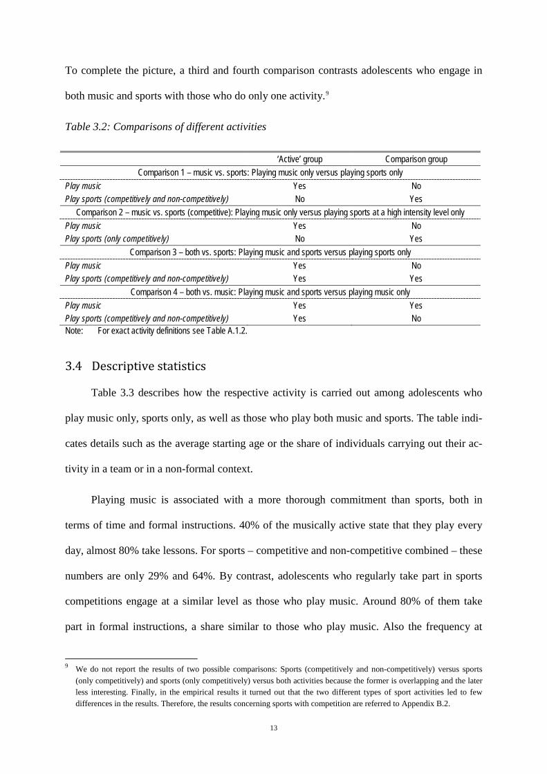
To complete the picture, a third and fourth comparison contrasts adolescents who engage in

both music and sports with those who do only one activity.9

Table 3.2: Comparisons of different activities

‘Active’ group Comparison group Comparison 1 – music vs. sports: Playing music only versus playing sports only

Play music Yes No Play sports (competitively and non-competitively) No Yes

Comparison 2 – music vs. sports (competitive): Playing music only versus playing sports at a high intensity level only Play music Yes No Play sports (only competitively) No Yes

Comparison 3 – both vs. sports: Playing music and sports versus playing sports only Play music Yes No Play sports (competitively and non-competitively) Yes Yes

Comparison 4 – both vs. music: Playing music and sports versus playing music only Play music Yes Yes Play sports (competitively and non-competitively) Yes No Note: For exact activity definitions see Table A.1.2.

3.4 Descriptive statistics

Table 3.3 describes how the respective activity is carried out among adolescents who

play music only, sports only, as well as those who play both music and sports. The table indi-

cates details such as the average starting age or the share of individuals carrying out their ac-

tivity in a team or in a non-formal context.

Playing music is associated with a more thorough commitment than sports, both in

terms of time and formal instructions. 40% of the musically active state that they play every

day, almost 80% take lessons. For sports – competitive and non-competitive combined – these

numbers are only 29% and 64%. By contrast, adolescents who regularly take part in sports

competitions engage at a similar level as those who play music. Around 80% of them take

part in formal instructions, a share similar to those who play music. Also the frequency at

9 We do not report the results of two possible comparisons: Sports (competitively and non-competitively) versus sports

(only competitively) and sports (only competitively) versus both activities because the former is overlapping and the later less interesting. Finally, in the empirical results it turned out that the two different types of sport activities led to few differences in the results. Therefore, the results concerning sports with competition are referred to Appendix B.2.

14

which the respective activity is carried out is comparable between music and competitive

sports participants.

Table 3.3: Characteristics of musical and athletic activities

Music only

Sports only (com-petitive and non-

competitive) Competitive sports only

Both: music + sports (competitive and non-competitive)

music sports (1) (2) (3) (4) Average starting age 8.8 9.1 8.6 8.6 9.1 Share doing sports/music in team (%) 53 63 79 52 59 Share with lessons/instructions (%) 79 64 83 78 67 Share playing sports/music daily (%) 40 29 37 38 29 Number of adolescents in sample 333 1640 884 501

Note: SOEP v29, 2001-2012, own calculations. Column (3) is a subgroup of column (2), otherwise each column contains distinct individuals, who carry out either music (1), sports (2 with subgroup 3) or both (4). The exact definitions of sports and music participation are given in Table A.1.2. Separate tables by gender can be found in the appendix (Tables A.2.3 and A.2.4).

One would think that engaging in both music and sports reduces the level of commit-

ment an adolescent is willing to dedicate to each of these activities. However, as described in

column (4) of Table 3.3, adolescents active in both activities are just as likely to play music

and sports daily or to take part in formal lessons as those who only participate in one activity.

Thus, for them, music and sports seem to be rather complements than substitutes.

In addition to differences related to the level of intensity, adolescents who play sports

start to become active at a later age and are more likely to play in a team than those who play

music. Team sports are particularly prevalent among boys and among those who regularly

participate at competitions.10 While only slightly more than half of the musically active

adolescents play music with other people (in an orchestra or a band), almost 80% of those

who do sports competitively take part in team sports.

Table 3.4 shows the distribution of the most important sports types among those who

play sports according to the various definitions described above. All numbers indicate the

percentage of adolescents who state to play the type of sports defined in the first column 10 Other than the higher share of boys carrying out team sports, there are no important gender differences in the

characteristics of music and sports participation (see Table A.2.3).

15

among the group of adolescents defined in the column heading. Unsurprisingly, soccer and

handball are typical sports that are carried out in competitions. On the contrary, fitness train-

ing, biking, swimming and walking are usually carried out alone, as indicated by the lower

share among adolescents taking part in sports competitions.

Table 3.4: Types of sports (in % of all sports)

Sports

(competitive and non-competitive)

Sports (competitive)

Sports (in addition to music,

competitive and non-competitive) (1) (2) (3)

Basketball 4.4 3.6 4.0 Bicycling 5.0 0.6 5.4 Dancing (except ballet) 5.5 4.8 9.6 Equestrian sport 5.4 4.3 8.2 Fitness training 2.2 0.1 2.0 Handball 5.2 8.5 4.8 Jogging 3.8 1.3 3.8 Soccer 31.2 41.5 15.2 Swimming, diving 5.2 2.5 5.4 Volleyball 4.9 5.6 8.4

Note: SOEP v29, 2001-2012, own calculations. The table shows the percentage of adolescents who state to play the type of sports defined in the first column among the group of adolescents defined in the column heading. The exact definitions of sports participation are given in Table A.1.2. Separate tables by gender can be found in the appendix (Tables A.2.5 and A.2.6).

There are clear gender differences with respect to the most important types of sports

(see Table A.2.4). Almost 60% of all boys who regularly take part in sports competitions

name soccer as their main sport. The most important sports types among girls are dancing,

equestrian sports and volleyball, each being considered as most important for more than 10%

of female sports participants. However, the relative importance of sports types is similar

among boys and girls, irrespective of whether sports is carried out in a competitive environ-

ment or whether music is played in addition.

Column (3) of Table 3.4 lists the most preferred sports types of adolescents who play

sports in addition to music. Given that these include individuals who take part in competitions

and those who do not, the distribution is relatively similar to that of column (1). However,

female sports (dancing, equestrian sports and volleyball) are overrepresented, and soccer is

16

underrepresented among the group of adolescents active in both sports and music. This is con-

sistent with the observation that adolescents who play music and sports are considerably more

likely to be female than adolescents who play sports only, as described in the following.

Table 3.5: Selected descriptive statistics by treatment status

Not

active

One activity Both

activities Sports (competi-

tive and non-competitive)

Sports (competitive

only)

Music

Characteristics Female (%) 55 41 35 59 56 At least one parent with university degree (%) 19 31 35 47 51 Average monthly labour market income of parents present in household (EUR) 1181 1443 1512 1681 1920

Household lives in rural area (%) 28 24 24 29 22 Mother’s conscientiousness (scale from 0 to 1) 0.87 0.87 0.87 0.86 0.85 Recommendation for upper secondary school (%) 25 38 44 55 68

Outcomes Adolescent attends upper secondary school (%) 23 38 44 57 66 Adolescent repeated a class (%) 27 22 20 14 09 Average grade (higher grade is better) -0.15 -0.02 0.01 0.20 0.32 Average cognitive skills -0.24 0.00 0.13 0.19 0.36 Conscientiousness -0.09 0.03 0.03 -0.05 0.13 Perceived control -0.16 0.06 0.17 0.10 0.18 Preference for the present 0.15 0.00 0.07 -0.11 -0.21

Note: SOEP v29, 2001-2012, own calculations. The exact definitions of each activity are given in Table A.1.2. All out-come variables except the first two are normalised to have mean 0 and a standard deviation of 1 for the entire sample. Tables with all covariates and outcomes can be found in the appendix (Tables A.2.1 and A.2.2).

As one might expect, adolescents who engage with music differ with respect to back-

ground characteristics and outcomes from inactive individuals, as well as from those who

engage with sports. Table 3.5 illustrates these differences. As stated above, the share of girls

is higher among adolescents who play both music and sports than among those who only play

sports. Moreover, adolescents who play sports usually come from social backgrounds that are

less advantaged than those of the musically active youth, but more advantaged than those of

individuals who play neither sports nor music. For example, in 47% of the families of musi-

cally active adolescents, at least one parent has a university degree, while this is true only for

31% of the athletically active’s families and for 19% of the parents among inactive individu-

als.

17

The same pattern between musically active, athletically active and inactive adolescents

is observed with respect to educational achievements and cognitive skills. For example, 57%

of the adolescents who play music attend an upper secondary school (Gymnasium), whereas

only 38% of those who play sports and 23% of those who are not active do so.

Furthermore, more competitively active adolescents come from a more favourable so-

cial background than those who are less involved. Individuals, who are engaged in sports at a

high intensity level (who regularly take part in sports competitions), are more similar to those

who play music than those who do sports at a lower level of intensity. Most remarkably, ado-

lescents active in both music and sports have wealthier and more educated parents than all

other groups of adolescents.

With respect to non-cognitive skills, adolescents who play music, sports or none of the

two are rather similar, both when comparing their parents and when comparing themselves.

The Big Five personality traits of mothers and fathers are almost identical along all activity

types. For the adolescents themselves, the only notable difference concerns the individual’s

time preference: Adolescents who play music have a lower preference for the present.

4 Econometrics

4.1 Identification

This paper investigates the differential impact of practicing sports or music during

childhood on the development of various skills, health, and personality traits. The challenge

for identifying causal differences is related to the fact that the decision to play music rather

than doing sports is not made randomly. We therefore have to disentangle the effect of par-

ticipating in a specific activity from the influence of differences in socio-demographic and

other background characteristics, given participation in at least one of those activities. In other

words, we need to take into account selection effects involved in comparing adolescents car-

18

rying out one or the other activity (or both). Given that we are not aware of any specific exog-

enous institutional features that could be used for identification (like in a difference-in-differ-

ence or regression discontinuity design), the potential identification strategies are either based

on instrumental variables type of assumptions or on assuming selection-on-observables. We

discuss both options in turn.

As described above, the SOEP contains rich socio-demographic information on the ad-

olescents and their parents. Therefore, selection-on-observables is an attractive identification

strategy. The main requirement is that we are able to control for all variables affecting treat-

ment (sports or music participation) and outcomes simultaneously, given participation in at

least one of the activities. If we assume that the decision process is a two-stage process in

which the first stage is a decision to be active or not, and the second stage is about the type of

activity, the potentially selective decision to take up music or sports practice rather than not

being active at all does not play any role for the identification of the effects of such compari-

sons.

To justify selection-on-observables as a strategy to identify causal effects, we need to

discuss the determinants of choosing between music and sports, or even carrying out both at

once. The choice of engaging with either activity can be motivated by taste, and expected

costs and gains. Moreover, there might be constraints hindering a child to pursue the activity

of interest. Finally, we only observe adolescents who play music or sports at age 17.Since we

consider adolescents as active if they started their activity at age 14 or earlier, being in the

‘treatment group’ also depends on the adolescent’s willingness to pursue the activity until age

17. In the following, we discuss the driving factors for each of these dimensions, as well as

how they might differ between music and sports. Moreover, we explain how our identification

strategy takes these potential confounders into account.

19

The choice to start music or/and sports activities can be considered as a common deci-

sion by child and parents. The decision most likely depends on utility gains and taste (Hille

and Schupp 2015). In addition to current pleasure, the former includes the desire to invest in

the child’s future skills (Eide and Ronan 2001, Lareau 2011). A priori, neither parents nor

child can judge which activity more effectively provides pleasure or stimulates skill develop-

ment. Therefore, they can only form their opinion according to their own experience and taste

and the information obtained from others (usually friends). These factors are approximated by

socio-economic status (Garboua and Montmarquette 1996).

Even more than sports, high-brow cultural activities such as playing music can be used

by individuals from higher social classes as a costly signal to assert their status (Menninghaus

2011, Ormel et al. 1999). A similar argument could justify the desire of parents to enrol their

child for two activities rather than one. Similarly, music might be played more often by ado-

lescents from particular socio-economic groups, because the offer of artistic activities for

children might be adapted to the tastes of the more highly educated (Lunn and Kelly 2009).

To take these determinants into account, we control for the parents’ socio-economic

background, which reflects both their eagerness to invest in the child’s future skills, as well as

their taste. We hold socio-economic background constant by controlling for the parents’ level

of education and income, as well as detailed information about the job they carried out when

the adolescent was 17 years old.11 The latter includes both parents’ work hours, their sector of

activity, whether their job required training, as well as their socio-economic status. In addition

to these objective indicators, parenting style is likely to affect the motivation to invest in the

child’s skill development. We proxy parenting style by controlling for the Big Five personal-

ity traits of mother and father, as well as an indicator of their willingness to take risks.12 Fi-

11 A list of all the variables used is available in the Table A.2.1 of the Appendix.

12 Ideally, to avoid that covariates are influenced by participation in music or sports, we would have liked to include the parents’ Big Five from before the child started doing music or sports. Unfortunately, personality questions have only been

20

nally, since ethnicity is an important determinant of socio-economic status and taste, we in-

clude the information on the possible migration background of the parents.

Even though willing to enrol their child at the local music school or sports club, parents

might face constraints hindering them to do so. Gustafson and Rhodes (2006) point out that

extracurricular activities require parental support, both financially and logistically. Parents

might face financial constraints if they cannot or do not want to afford the costs for lessons,

club membership, as well as musical instruments or sports equipment. Moreover, parents

might not be able to provide the necessary logistical support, especially if they have other

children or work full-time (Lareau 2011). Also, the child’s position in the birth order plays an

important role for the educational investments made by the parents (Black, Devereux and Sal-

vanes 2005).

For most parents in Germany, financial constraints are unlikely to be the crucial deter-

minant of the decision to sign up at a music school or sports club. Among families with chil-

dren, 57% report that they have regular expenses for non-formal educational activities. On

average, these families spend 51 EUR per month for the athletic and musical activities of their

children (Schröder, Spieß and Storck 2015). Concerning expenditures for music, fees vary

strongly between music schools and have accounted for 47 percent of the overall budget of

German public music schools in 2013 (MIZ 2014).13 However, the German association of

public music schools (Verband deutscher Musikschulen) stipulates that their members should

provide reduced fees for children from poor families (VDM 2011). In contrast, membership

fees in sports clubs are very low on average. For adolescents, the median membership fee was

just 3.10 euros per month in 2013 (Breuer and Feiler 2015). In addition, the “Educational

package” – a policy introduced by the German federal government in 2011 – subsidizes

asked in the SOEP individual questionnaire in 2005 and 2009. However, we do not worry about the timing of the measurements because personality is considered to be stable among adults (Pervin, Cervone and John 2005).

13 Another 48% of their revenues stems from public subsidies (MIZ 2014).

21

membership fees in sports clubs or music schools for poor families in the amount of 10 euros

per month (BMAS 2015).

The extent to which the abovementioned constraints vary between music and sports de-

pends on factors such as household income, the number of children in the household and birth

order, but also on the institutional context in which the activity is carried out. We control di-

rectly for the first three factors, whereas the latter cannot be observed in our data. Depending

on living area and time, as well as the organizational structure of the local music school or

sports club, material investments might be more substantial for music or for sports. We ap-

proximate these factors by including state and birth year fixed effects, as well as an indicator

of whether the household lives in a rural area.

To be observed as either playing sports or music, adolescents in our sample need to pur-

sue these activities until they answer the SOEP Youth Questionnaire at age 17. In addition to

motivation and constraints, the willingness not to give up before age 17 therefore constitutes

an important dimension in the non-random selection into one of the activity groups. Whether

an individual gives up music or sports during adolescence is likely to depend on encourage-

ment by the parents, as well as own motivation, the opportunity costs of time, and the per-

ceived returns in general. According to Farrell and Shields (2002) and Raudsepp (2006), par-

ents as role models can motivate children to play music and sports, and might determine

whether they pursue these activities until age 17. Whether parental encouragement leads the

child to prefer music to sports probably depends on parental taste, which we control for as

explained above.

Moreover, carrying out music or sports throughout adolescence requires motivation and

time. Adolescents who struggle at school are unlikely to be able to dedicate time to these ac-

tivities in their leisure time. The individual characteristics determining whether adolescents

can pursue their extracurricular activities are difficult to take into account, given that we ob-

22

serve only few individual characteristics before the age of 17. To approximate these charac-

teristics, we control for gender and an indicator whether the adolescent has received a recom-

mendation for upper secondary school by her primary school teacher (in grade 4, at age 9 to

10). The latter serves as a proxy for ability. Furthermore, if the remaining unobserved reasons

for giving up sports and music before the age of 17 are similar, this does not pose a threat to

identification.

Several reviews investigate the determinants and correlates of physical activity among

children and adolescents in empirical studies (Craggs et al. 2011, van der Horst et al. 2007,

Sallis, Prochaska and Taylor 2000). They underline two points: i) the determinants vary be-

tween children (aged 4 to 12 years old) and adolescents (aged 13 to 18 years old), and ii) the

identification of the determinants of a change in physical activity levels often suffers from re-

verse causality. Our study focuses on individuals who decided to engage or to quit sport while

being children and then adolescents. Therefore, we are interested in determinants of sports

and of a change of the sports activity for both age categories. Previous findings on these de-

terminants are consistent with the arguments described above. Light (2010) suggests that

friendship is an important determinant of the child’s decision to remain in a competitive club.

We cannot control for such individual characteristics. However, as mentioned above, there is

a potential reverse causality issue that would have prevented us to use such information as a

control. Moreover, we believe that these unobserved factors are similar for music and sports.

An alternative identification strategy is instrumental variables (IV). A crucial charac-

teristic of a valid instrument is that it affects educational outcomes only by affecting music

and/or sports participation (the so-called exclusion condition). Indeed some of the commonly

used instruments (e.g. height or school characteristics) may be questionable in this respect.14

14 Instrumental variables used to handle selection problems in sports economics are schools characteristics (Anderson 2001,

Barron, Ewing and Waddell 2000), height (Eide and Ronan 2001, Rees and Sabia 2010) and distance to sports infrastructures (e.g. as a robustness check in Felfe, Lechner and Steinmayr 2011).

23

Therefore, we use an alternative instrument, namely parental artistic activities, which argua-

bly fulfil the requirements for an IV. They are a strong predictor for adolescents’ music par-

ticipation and – conditioning on further covariates – unlikely to directly influence the out-

comes. However, this instrument is not available for the entire sample, which implies a further

reduction of the number of observations, which in turn drastically reduces the precision of the

estimates. Therefore, we will use this IV as a robustness check only.15

4.2 Estimation

Our study compares the effects of different activities with each other. This corresponds

to the multiple treatment setting discussed in Imbens (2000) and Lechner (2001). Therefore,

the sample reduction results of Lechner (2001) apply. Thus, to estimate the effects of one ac-

tivity compared to another by a selection-on-observables approach, participants in activity

groups other than those two under explicit consideration are deleted for the purpose of this

particular estimation. For example, for the estimation of the effect of being active in sport

compared to music, individuals who do both activities play no role.

For performing the pairwise comparisons, we use the propensity score matching esti-

mator proposed by Lechner, Miquel and Wunsch (2011). This estimator performed well in the

large-scale simulation study by Huber, Lechner and Wunsch (2013). It is described in detail in

Appendix C. Such semi-parametric estimators are based on estimating a parametric model

(e.g. probit) for the probability of belonging to one of the groups compared to another, condi-

tional on the above mentioned control variables. The relation between the outcomes, activity

types, and confounders, however, are left unspecified (non-parametric). Therefore, such esti-

mators have the advantage that they allow for very flexible effect heterogeneity (contrary to

regression models, for example).

15 Results based in this instrument as well as the extensive arguments why it is probably valid are contained in Appendix D.

24

For each outcome variable, having four groups of activity (music, sports, competitive

sports and both) leads to up to 6 different estimates for each treatment effect, like the average

treatment effect (ATE), the average treatment effect on the treated (ATET) and the average

treatment effect on the non-treated (ATENT). However, an implication of treating the estima-

tion problem as many single pair-wise problems is that the reference population for these ef-

fects is specific to each single comparison. For example, the standard ATE refers to the union

of the respective treatment and control groups in the particular comparison. However, the

characteristics of those groups will not be the same for different comparisons. Therefore, we

follow the approach advocated and implemented by Lechner and Wunsch (2009) in a similar

situation to keep the ‘target’ or ‘reference’ distribution the same for the different comparisons.

In this case, there is an additional matching step. Matching is performed such that the implied

weighting scheme leads to matched covariate distributions of treated and controls in all com-

parisons that resemble those in the ‘target’ population. Thus, the various estimation results

presented below always refer to the same population (and thus the same distribution of con-

founding characteristics) and thus are comparable in that sense. In our case, a natural candi-

date for the target population is the union of sports and music participants.

5 Results

5.1 Propensity scores

We investigate the differential effects of music and sports in this paper by examining

the consequences of playing music instead of doing sports, as well as playing music and

sports instead of doing one activity only. All estimations were carried out separately for four

comparisons. These comparisons were chosen with the aim to distinguish between two types

of outcome differences: i) the effects resulting from playing music rather than sports, and ii)

25

the effects related to being active at different levels of intensity. Detailed definitions of the

treatment and control group for each comparison are given in Table 3.2.

Table 5.1 shows the average marginal effects of the estimation of the propensity score

for three of these four comparisons for selected covariates.16 Since the results for competitive

sports are very similar to sports in general, these results are referred to Appendix B. Gener-

ally, the results confirm the (unconditional) summary statistics of Section 3.4. Adolescents

who engage with music tend to come from more advantaged social backgrounds. Still, paren-

tal education plays a much smaller role in choosing between sports and music than in the gen-

eral decision to become musically or athletically active. Note that parental income is not sta-

tistically significant and that other parental characteristics play only a minor role. For exam-

ple, a higher willingness to take risks among parents is associated with a lower probability

that their child plays music rather than sports. The strong effect of openness both for mothers

and fathers can be explained with the fact that openness towards artistic experiences is used as

one of the items assessing this personality dimension.

Two important predictors of playing music rather than sports are the adolescent’s gen-

der and whether she or he received a recommendation for upper secondary school at the end

of primary school. Girls are 10% more likely to play music instead of or in addition to sports

than boys, all other covariates held constant. As a proxy for prior abilities, the recommenda-

tion for upper secondary school is especially important in determining who carries out two

activities rather than one. The probability to play music and sports rather than just one of the

two is 14% higher among adolescents who received such a recommendation.

16 All covariates have a small number of missing observations (around 5% for most covariates). To account for non-

randomness among the missing observations, we include indicators which turn on if at least one variable in a group of similar covariates is missing. The missing covariate value is coded to 0 for binary variables and to the mean of the non-missing observations otherwise.

26

Table 5.1: Selected results of propensity score estimation

Music only

vs. sport only

Music + sport

vs. sport only

Music + sport vs.

music only (1) (3) ()

Marginal effects

p-value in % Marginal

effects p-value

in % Marginal effects

p-value in %

Female 0.106 0 0.096 0 -0.035 31 Recommendation for upper secondary school 0.044 2 0.148 0 0.141 0 Birth order -0.033 1 -0.040 0 0.004 88 Number of siblings in SOEP 0.023 1 0.032 0 0.011 49 Household lives in rural area 0.039 10 0.011 65 -0.055 23 Monthly labour market income of parents who live in household -0.001 88 0.005 61 0.017 33

Working hours (mother) -0.001 22 -0.002 2 -0.001 59 Working hours (father) 0.001 13 0.002 3 0.001 71 Willingness to take risks (mother) -0.008 7 -0.008 7 0.005 61 Willingness to take risks (father) -0.011 2 -0.011 2 0.002 80 At least one parent with … university degree 0.004 90 0.048 7 0.035 54

… upper secondary schooling degree 0.039 14 0.033 21 -0.038 47 … migration background -0.023 36 0.027 29 0.078 13 Big Five (mother) - Agreeableness -0.162 3 -0.129 9 0.130 45 - Conscientiousness 0.010 91 -0.092 30 -0.243 19 - Extraversion -0.081 22 -0.088 24 -0.041 78 - Neuroticism -0.025 67 -0.042 48 -0.058 62 - Openness 0.142 2 0.120 8 -0.065 63 Big Five (Father)- Agreeableness 0.079 32 0.124 12 0.054 71 - Conscientiousness 0.048 57 0.120 18 0.179 35 - Extraversion -0.072 30 -0.077 30 0.059 68 - Neuroticism 0.157 1 0.087 15 -0.099 44 - Openness 0.141 6 0.172 3 -0.034 82 Efron’s R2 (in %) 11 16 7 Number of observations 1973 2141 834

Note: SOEP v29, 2001-2012, own calculations. Probit model estimated. Average marginal effects presented. Inference is based on 4999 bootstrap replications. Numbers in italics / bold / bold italics indicate significance at the 10% / 5% / 1% level. The exact definitions of each activity (dependent variable) are given in Table 3.2 and A.1.2. The following are also included in this specification: Constant term, year of birth, single parent household, dummies for the fed-eral states, household net overall wealth, age of mother at birth, indicators for mothers working in services, fathers working in services, mothers working in manufacturing or agriculture, fathers working in manufacturing or agricul-ture, at least one parent with vocational degree, ISEI socio-economic status (‘higher’ for both parents), current job did not require training (mother), current job did not require training (father), indicators for missing values in willing-ness to take risks (mother), and willingness to take risks (father). The full results are given in Appendix B (Table B.1.1).

Using the coefficients from Table 5.1, we predict the probability for each individual to

belong to the respective activity group. In order to eliminate differences in covariate distri-

butions between the groups, we match both groups on the propensity score and on gender (to

fully remove all gender difference that deem to be particularly important in this application),

27

as described in Section 4.2. After matching, all covariates are balanced (see Table B.1.2). The

cut-off for the common support with respect to the target distribution is the 99% quantile of

the respective propensity score distribution. Different cut-off values are considered as robust-

ness check (more details are given in section 5.4. on robustness check).

5.2 Effects of music compared to sports

Table 5.2 shows the average effects for the four contrasts of music and sports described

in the previous section.17 In all comparisons, the results are reweighted with respect to the

characteristics of adolescents who are active in music or sports or both, as described in section

4.2.18 While Table 5.2 displays the key outcome variables, Appendix B.2 contains results for

the additional outcomes. It also contains the results for the comparison of music versus com-

petitive sports, because those results turned out to be very similar to the ones that included all

types of sports and thus removed from the tables in the main body of the text.

Column (1) of Table 5.2 presents effects of playing music only compared to doing

sports only: Musically active adolescents obtain better school grades in languages, scoring

about one sixth of a standard deviation above athletically active adolescents. This tendency of

music leading to better skills exists for most of the school achievement and cognitive skills

variables, although these differences are not always statistically significant. Furthermore, ad-

olescents who play music are eight percent more likely than sports participants to attend upper

secondary school, and ten percent more likely to aim at going to university.

17 Further results in particular about further personality traits are referred to Appendix B for the sake of brevity. Note also

that cognitive skills as well as some non-cognitive skills (e.g. Big Five personality traits and risk aversion) were only measured from 2006 onwards (Weinhardt and Schupp 2011), while all other outcomes were available from 2001 onwards. Thus, for those variables, the sample size is considerably smaller and the results refer to the later period only. Whether an individual is part of this later subsample is essentially determined by the adolescent's year of birth.

18 However, the results are similar if we weight them according to the characteristics of the overall population of active and inactive individuals (see Table B.3.9).

28

When comparing the results for doing both activities to only one of them (columns 2

and 3), the results for the educational outcomes show that doing both activities jointly is more

beneficial than just a single one. For example, adolescents playing both music and sports out-

perform those who only play sports by more than one fifth of a standard deviation in the cog-

nitive skills test. This effect is similarly positive in comparison to those who play music only.

In addition, individuals active in music and sports have better school grades, although only

one of the four grade effects is significantly different from zero for each comparison.19

As described in Section 3.4, adolescents who play music and sports carry out each ac-

tivity with a time commitment similar to those who are only active in one of them. Irrespec-

tive of potential benefits from music or sports, playing both activities might impede school

achievement due to the large amount of time spent on this extracurricular involvement. How-

ever, the abovementioned results suggest that on average doing both activities does not put so

much strain on the adolescents as to negatively affect their educational success, but quite the

opposite.

With respect to personality, we observe several statistically significant differences be-

tween musically and athletically active adolescents. The positive effect of music on openness

is statistically significant and substantial at more than one third of a standard deviation. This

is related to the fact that openness to artistic experiences is one of the three items assessing

this personality dimension in our data. Musically active adolescents are less willing to take

risks than those who play sports. Finally, adolescents who do sports in addition to music are

more than one quarter of a standard deviation more extravert than those who play music only.

19 However, comparing adolescents who play both music and sports to those who only do one activity involves a more

important risk of selection based on unobservable characteristics than the single-activity comparisons described above. Being this much engaged in extracurricular activities requires particular investments. Students with weak school performance or students who have work after school will probably not find the necessary time to play music and sports. Let alone the particular financial and emotional support that is necessary from parents and teachers.

29

Table 5.2: Average effects of music vs. sports

Music only vs.

sport only

Music + sport vs.

sport only

Music + sport vs.

music only (1) (3) (4)

Outcome variables Effect p-value in %

Effect p-value in %

Effect p-value in %

Cognitive skills and school achievements at age 17 Cognitive skills - Average 0.012 90 0.233 1 0.230 5 - Analogies 0.054 58 0.216 1 0.169 15 - Figures 0.053 59 0.276 0 0.229 5 - Math -0.045 63 0.070 45 0.123 30 School grades - Average 0.034 66 0.151 3 0.123 20 - Maths -0.119 14 0.113 12 0.233 2 - German 0.172 2 0.113 11 -0.051 59 - 1st for. lang. 0.063 42 0.103 13 0.046 63 Attends upper secondary school 0.081 4 0.135 0 0.063 18 Aim to enrol at university 0.106 1 0.187 0 0.087 6 Attends university at age 20 0.024 48 0.084 1 0.065 13

Personality at age 17 Big 5: Conscientiousness -0.114 21 0.059 51 0.165 14 Extraversion -0.165 9 0.128 13 0.294 1 Neuroticism 0.103 31 0.013 88 -0.090 47 Openness 0.407 0 0.349 0 -0.058 63 Agreeableness 0.048 60 0.206 2 0.152 17 Willingness to take risk -0.211 4 -0.181 6 0.021 87

Subjective health and life style at age 18 Satisfaction with health -0.119 45 -0.143 28 -0.050 80 Current health situation -0.138 4 -0.048 39 0.083 30 Currently smoking -0.007 88 -0.110 0 -0.107 5

Other leisure activities at age 17 Watching TV daily -0.099 0 -0.115 0 -0.016 71 Playing computer games daily -0.075 2 -0.044 14 0.029 47 Reading daily 0.067 5 0.127 0 0.062 14 Note: Effects presented are average treatment effects for the target population. Inference is based on 4999 bootstrap

replications. Numbers in italics / bold / bold italics indicate significance at the 10% / 5% / 1% level. The measure-ment of all outcomes is described in Table E.1. School grades, cognitive skills and personality are normalised to mean zero and variance 1 (higher value of grades is better). All other outcome variables are binary, except for ‘satisfaction with health’ (0 “worst” to 10 “best”) and ‘current health situation’ (1 “bad” to 5 “very good”). The full set of results is contained in Table B.2.1 in Appendix B.2.

The third block of results in Table 5.2 shows that being athletically active leads to im-

proved health outcomes. Adolescents who play sports in addition to or instead of music are

more satisfied with their health and also report a better subjective health status. Of course,

given our data, it remains a somewhat open, although maybe philosophical question whether

this gain in subjective health translates into objective health measures of this young popula-

tion (which is of course healthier than the population at large). Considering additional effects

of doing two activities versus one, it turns out that adolescents who do both activities are ten

percent less likely to smoke than whose who only done of those activities.

30

Finally, adolescents active in music and sports differ with respect to their leisure time

occupations, as described in the lower panel of Table 5.2. Adolescents who play music are

more likely to read and less likely to watch TV or play computer games every day than those

doing sports. If we believe that playing computer games and watching TV is on average not

supportive of educational success while reading fosters it, then these results are in line with

the findings for the educational outcomes and may provide at least a partial explanation of

these findings.

5.3 Heterogeneity

Next, we investigate heterogeneities in the effects for different subgroups of the target

population with respect to gender and socio-economic background (for detailed results see

Tables B.3.1 to B.3.9 in Appendix B). According to the literature as well as to the descriptive

statistics shown in Section 3.4, male and female sports are different. Our main results take this

specificity into account by matching adolescents by gender (but of course subsequently aver-

aging their effects). In the following, we estimate the outcome differences between musically

and athletically active adolescents for each gender separately to understand gender-specific

differences between both activities. Before going into detail, note however that most of the

following comparisons, documented in Appendix B.3, suffer from a loss of power, the mag-

nitude of which varies between small and substantial. This loss is due to the reduced sample

sizes within the additional strata.

With respect to cognitive skills and school grades, music seems to be more beneficial

for girls, while sports may rather help boys. Girls see their language-related skills and grades

improve by one fourth of a standard deviation when playing music, while athletically active

boy obtain better results in mathematics. Other differences between music and sports are

driven by male adolescents only. The positive effect of music on ambition is stronger for

31

males than for females. Finally, male sports participants increase their degree of extraversion

compared to male musicians. This difference cannot be observed among women.

In order to investigate outcome differences between music and sports for different levels

of socio-economic status, we estimated these differences in various subgroups. These sub-

groups stratify the full sample by parental labour market income, parental education, as well

as the adolescent’s abilities, as measured by the recommendation for upper secondary school

received from their primary school teacher. In summary, we find that adolescents with richer

or more highly educated parents, as well as adolescents with higher ability, have an advantage

from playing music rather than sports for a variety of outcomes. For them, music is associated

with higher cognitive skills and school grades. This is even more the case if the adolescent is

active in two activities rather than one. In other words, while music and sports are similarly

beneficial for children from disadvantaged social backgrounds, those from richer and more

highly educated families do better with music than with sports. They also do better with two

rather than one activity. One possible explanation relates to Bourdieu’s cultural reproduction

hypothesis. According to Bourdieu and Passeron (1990), parents from higher socio-economic

status have access to better quality cultural education, leading their children to more strongly

benefit from playing music.

5.4 Robustness

One advantage of propensity score matching in comparison to OLS is related to the pos-

sibility to verify the common support between treatment and control group. If both groups are

very different in their covariates, linear estimations might be sensitive to minor changes in the

specification (Imbens, 2014). All our estimations have common support along the distribution

of the propensity score between treatment and control groups as well as the target population.

Even though we control for a large number of individual and parental background character-

32

istics, we can identify control observations along the entire distribution of propensity scores in

the treatment group, and vice versa.

Our estimations are robust to various modifications in treatment definition and estima-

tion method. For example, all effects are slightly stronger if we restrict the sample of musi-

cally active adolescents to those who take music lessons outside of school. Moreover, our

results are robust to the alternative definitions of being active in music or sports, in which we

disregard those who state to be active less than once a month. The results of these estimations

are presented in Tables B.4.1 and B.4.2 in Appendix B.

We also checked the robustness of the results with respect to the particular method used

for the bias correction step in the matching estimator.20 It turns out that, here, the bias correc-

tion does not matter. Similarly, varying the criteria to define the common support from 99%

to 97% does not change in any relevant way (see Table B.4.3).

Panel attrition and item non-response do not appear to threaten our results either. We

check this by creating on additional outcome variable measuring non-response. The effects on

this missing indicator are small and statistically insignificant (see Table B. 4.4). In addition,

the results are robust to using survey weights or not (see Table B.4.5).

We believe that the large number of informative and relevant individual and family

characteristics included in our estimations is likely to make the conditional independence as-

sumption (CIA) plausible. Thus our estimates have a causal interpretation. Still, we cannot en-

tirely exclude the possibility that unobserved characteristics determine the choice between

music and sports and simultaneously affect adolescents’ outcomes. Although, of course, the

CIA cannot be empirically tested in a statistical sense, we run two plausibility tests to shed

some light on the potential validity of this assumption and the effects of deviating from it.

First, we used an instrumental variable to model the choice between music and sports.

As instrument, we took an indicator of whether either parent played a musical instrument in 20 Results are available on request; all tables presented in this paper are based on a linear bias correction.

33

their youth. This instrument arguably has no direct impact on children’s outcome other than

influencing the parents’ taste with respect to their child’s leisure activity conditional on the

covariates (for a more detailed discussion, see Appendix D). The empirical results do not

contradict our main findings. However, this test is not very powerful, because the IV results

are subject to substantial sampling noise.

Second, we ran the formal sensitivity test as developed by Ichino, Mealli and Nannicini

(2008) and implemented by Lechner and Downward (2013). This test is based on a simulation

exercise to evaluate the sensitivity of the results with respect to potential violations of the

CIA. It turns out that the results appear not to be sensitive to the investigated misspecifica-

tions (the details of the procedure used and the results are discussed in Appendix D.2).

6 Conclusions

Using the data of the German Socioeconomic Panel, this paper analyses the effects of

spending part for adolescents’ leisure time on playing music or doing sports, or both. Con-

centrating on those two competing uses of leisure time has the advantage of explicitly recog-

nising that doing one of those potentially beneficial activities may crowed out the other due to

lack of sufficient free time. Thus, the estimated effects have more obvious and useful inter-

pretation than in the previous literature that compared essentially each of those activities sepa-

rately to ‘not doing that particular activity’. There is also an econometric advantage, because

selection effects resulting from the parents’ or child’s decisions to spend time on one of these

major extracurricular activities are irrelevant. If selection into these activities can be thought

of as a two stage process, with a first stage decision on spending time and money on one of

the two, and a second stage decision about the particular type, then only the second stage is of

potential concern. Thus, identification will be greatly improved.

34

The main results indicate that the two activities may have indeed quite different impli-

cations. Playing music appears to foster academic performance and academic ambition com-

pared to doing sports, in particular for girls and children from more highly educated families.

It also goes along with additional time spent reading and less time spent on watching TV and

playing computer games. Doing sports on the other hand improves adolescents’ subjective

health. Since the positive effects on academic performance as well as the positive health

effects should improve future labour market performance (and life satisfaction), it is not clear

which of the two activities should be preferred, for example, by a parent interested in max-

imising life-time utility of their off-spring. Thus, there is no straightforward policy conclusion

on which of those two activities should be preferred by public policy (or parents). Interest-

ingly, when comparing the effects of doing both activities together against doing only one of

them, positive effects appear as well for doing both.

An extensive robustness analysis based on a semiparametric instrumental variable esti-

mation and a formal sensitivity analysis suggests that these results are robust with respect to

several possible violations of key identifying assumptions, as well as various plausible values

of the tuning parameters of the estimator.

An interesting avenue for future research consists in understanding the reasons (‘medi-

ators’) behind those findings. Such an endeavour will however require larger samples than the

ones available for the current study.

References

Anderson, D. (2001), “‘If You Let Me Play’: The Effects of Participation in High School Athletics on Students'

Educational and Labor Market Success”, SSRN.

Barron, J., B. Ewing, and G. Waddell (2000), “The effects of high school athletic participation on education and

labor market outcomes”, Review of Economics and Statistics, 82, 409-421.

35

Becker, G. (1965), “A Theory of the Allocation of Time”, Economic Journal, 75 (299), 493-517.

Besson, M., D. Schon, S. Moreno, A. Santos, and C. Magne (2007), “Influence of musical expertise and musical

training on pitch processing in music and language”, Restorative Neurology and Neuroscience, 25 (3-4), 399-

410.

Bialystok, E. and A.-M. DePape (2009), “Musical expertise, bilingualism, and executive functioning”, Journal of

Experimental Psychology, Human Perception and Performance, 35 (2), 565-574.

Bilhartz, T., R. Bruhn and J. Olson (1999), “The effect of early music training on child cognitive development”,

Journal of Applied Developmental Psychology, 20 (4), 615-636.

Black, S., P. Devereux and K. Salvanes (2005), “The More the Merrier? The Effect of Family Size and Birth

Order on Children's Education”, The Quarterly Journal of Economics, 120 (2), 669-700.

BMAS (2015), The educational package: A new start for taking part, Brochure, Federal Ministry of Labour and

Social Affairs.

Bourdieu, P., and J.-C. Passeron (1990), Reproduction in Education, Society and Culture, Vol. 4, SAGE Publi-

cations Limited.

Breuer, C., and S. Feiler (2015), „Sportvereine in Deutschland – ein Überblick“, in Breuer C., ed., Sportent-

wicklungsbericht 2013/2014. Analyse zur Situation der Sportvereine in Deutschland, Köln: Sportverlag

Strauß.

Cabane, C., and A. Clark (2013), “Childhood Sporting Activities and Adult Labor-Market Outcomes”, Paris

School of Economics Working Paper, 2013-34.

Cabane, C., and M. Lechner (2015), “Physical activity of adults: A survey of correlates, determinants, and ef-

fects”, forthcoming in Jahrbücher für Nationalökonomie und Statistic (Journal of Economics and Statistics).

Cobb-Clark, D., and S. Schurer (2012), “The stability of big-five personality traits”, Economics Letters, 115 (1),

11-15.

Covay, E., and W. Carbonaro (2010), “After the Bell: Participation in Extracurricular Activities, Classroom

Behavior, and Academic Achievement”, Sociology of Education, 83 (1), 20-45.

Craggs, C., K. Corder, E. M. F. van Sluijs and S. J. Griffin (2011). “Determinants of Change in Physical Activity

in Children and Adolescents – A Systematic Review”, American Journal of Preventive Medicine, 40(6), 645-

658

Dahmann, S., and S. Anger (2014), “The Impact of Education on Personality: Evidence from a German High

School Reform”, IZA Discussion Paper 8139.

Del Boca, D., C. Monfardini and C. Nicoletti (2012), “Children's and Parents' Time-Use Choice and Cognitive

Development during Adolescence”, Human Capital and Economic Opportunity Working Paper Series 2012-

006, University of Chicago.

Deutsche Sportjugend (2014), Deutsche Sportjugend, http://www.dsj.de/deutsche-sportjugend/, accessed Nov

4th, 2014.

Donnellan, M., and R. Lucas (2008), “Age differences in the big five across the life span: Evidence from two

national samples”, Psychology and Aging, 23 (3), 558-566.

36

Eccles, J., B. Barber, M. Stone, and J. Hunt (2003), “Extracurricular Activities and Adolescent Development”,

Journal of Social Issues, 59 (4), 865-889.

Eide, E., and N. Ronan (2001), “Is Participation in High School Athletics an Investment or a Consumption

Good? Evidence from High School and Beyond”, Economics of Education Review, 20, 431-442.

European Commission (2007), European Cultural Values, Special Eurobarometer 278,

http://ec.europa.eu/public_opinion/archives/ebs/ebs_278_en.pdf, accessed July 17th, 2014.

European Commission (2011), Youth on the move, Flash Eurobarometer #319a,

http://ec.europa.eu/public_opinion/flash/fl_319a_en.pdf, accessed July 17th, 2014.

European Commission (2014), European Cultural Values, Special Eurobarometer 412,

http://ec.europa.eu/health/nutrition_physical_activity/docs/ebs_412_en.pdf, accessed July 17th, 2014.

Eurostat (2009): Youth in Europe. A statistical portrait,

http://epp.eurostat.ec.europa.eu/cache/ITY_OFFPUB/KS-78-09-920/EN/KS-78-09-920-EN.PDF, accessed

July 17th, 2014.

Ewing, B. (2007), “The Labor Market Effects of High School Athletic Participation: Evidence From Wage and

Fringe Benefit Differentials”, Journal of Sports Economics, 8 (3), 255-265.

Farrell, L. and M. Shields (2002), “Investigating the Economic and Demographic Determinants of Sporting Par-

ticipation in England”, Journal of the Royal Statistical Society. Series A (Statistics in Society), 165 (2), 335-

348.

Feldman Farb, A., and J. Matjasko (2012), “Recent advances in research on school-based extracurricular activi-

ties and adolescent development”, Developmental Review, 32 (1), 1-48.

Felfe, C., M. Lechner and A. Steinmayr (2011), “Sport and Child Development”, Economics Working Paper

Series 1135, University of St. Gallen, School of Economics and Political Science.

Frölich, M. (2007), “Nonparametric IV estimation of local average treatment effects with covariates”, Journal of

Econometrics, 139 (1), 35 - 75.

Garboua, L., and C. Montmarquette (1996), “A microeconometric study of theatre demand”, Journal of Cultural

Economics, 20, 25-50.

Grgic, M., and I. Züchner (2013), Medien, Kultur und Sport bei jungen Menschen. Beltz Juventa.

Gustafson, S., and R. Rhodes (2006), “Parental Correlates of Physical Activity in Children and Early Adoles-

cents”, Sports Medicine, 36 (1), 79-97.

Heckman, J., and T. Kautz (2012), “Hard evidence on soft skills”, Labour Economics, 19, 451-464.

Hille, A., A. Arnold and J. Schupp (2014), “Leisure behavior of young people: Education-oriented activities

becoming increasingly prevalent”, DIW Economic Bulletin, 4 (1), 26-36.

Hille, A., and J. Schupp (2015), “How learning a musical instrument affects the development of skills”, Eco-

nomics of Education Review, 44, 56-82.

Ho, Y., M. Cheung, A. Chan and S. Chan (2003), “Music training improves verbal but not visual memory:

Cross-sectional and longitudinal explorations in children”, Neuropsychology, 17 (3), 439-450.

Hovemann, G., and P. Wicker, (2009), “Determinants of sport participation in the European Union”, European

Journal for Sport and Society, 6 (1), 51-59.

37

Huber, M., M. Lechner, and A. Steinmayr (2012), “Radius Matching on the Propensity Score with Bias Adjust-

ment: Finite Sample Behaviour, Tuning Parameters and Software Implementation”, Economics Working Pa-

per Series 1226, University of St. Gallen, School of Economics and Political Science.

Huber, M., M. Lechner, and C. Wunsch (2013), “The performance of estimators based on the propensity score”,

Journal of Econometrics, 175 (1), 1-21.

Ichino, A., F. Mealli and T. Nannicini (2008), “From Temporary Help Jobs to Permanent Employment: What

Can We Learn from Matching Estimators and their Sensitivity?”, Journal of Applied Econometrics, 23, 305-

332.

Imbens, G. (2000), “The role of the propensity score in estimating dose-response functions”, Biometrika, 87 (3),

706-710.

Imbens, G. (2014), “Matching methods in practice: Three examples”, IZA Discussion Paper 8049.

Lang, F., D. John, O. Lüdtke, J. Schupp and G. Wagner (2011), “Short assessment of the Big Five: robust across

survey methods except telephone interviewing”, Behavior Research Methods, 43 (2), 548-567.

Lareau, A. (2011), Unequal Childhoods: Class, Race, and Family Life, 2nd ed., University of California Press.

Lechner, M. (2001), “Identification and estimation of causal effects of multiple treatments under the conditional

independence assumption” in Lechner, M. and F. Pfeiffer, eds., Econometric Evaluation of Labour Market

Policies, Physica-Verlag HD, 43-58.

Lechner, M. (2009), “Long-run labour market and health effects of individual sports activities”, The Journal of

Health Economics, 28, 839–854.

Lechner, M., and C. Wunsch (2009), “Are Training Programs More Effective When Unemployment is High?”,

Journal of Labor Economics, 27 (4), 653-692.

Lechner, M., and N. Sari (2014), “Labor Market Effects of Sports and Exercise: Evidence from Canadian Panel

Data”, IZA Discussion Paper 7931.

Lechner, M., and P. Downward (2013), “Heterogeneous Sports Participation and Labour Market Outcomes in

England”, IZA Discussion Paper 7690.

Lechner, M., R. Miquel and C. Wunsch (2011), “Long-Run Effects of Public Sector Sponsored Training in West

Germany”, Journal of the European Economic Association, 9 (4), 742-784.

Light, R. L. (2010), “Children’s Social and Personal Development Trough Sport: A Case Study of an Australian

Swimming Club”, Journal of Sport & Social Issues, 34 (4), 379 - 395.

Lipscomb, S. (2007), “Secondary school extracurricular involvement and academic achievement: a fixed effects

approach”, Economics of Education Review, 26 (4), 463 - 472.

Long, J., and S. Caudill (1991), “The Impact of Participation in Intercollegiate Athletics on Income and Gradua-

tion”, The Review of Economics and Statistics, 73 (3), 525-31.

Loui, P., K. Kroog, J. Zuk, E. Winner, and G. Schlaug (2011), “Relating pitch awareness to phonemic awareness

in children: implications for tone-deafness and dyslexia”, Frontiers in Auditory Cognitive Neuroscience,

2(111), 1-5.

38

Lunn, P., and E. Kelly (2009), “Accounting for Taste: An Examination of Socioeconomic Gradients in Attend-

ance at Arts Events”, ESRI Working Paper 283, Economic and Social Research Institute (ESRI), Dub-

lin/Ireland.

McCrae, R., and P. Costa (1999), The Five Factor Theory of Personality, translated by John, O., R. Robins and

L. Pervin, Guilford, New York, 139-153.

Menninghaus, W. (2011) Wozu Kunst? Asthetik nach Darwin, Suhrkamp Berlin.

MIZ (2014), Einnahmen und Ausgaben der Musikschulen im VdM,

http://www.miz.org/intern/uploads/statistik125.pdf, accessed March 18th, 2015.

Nering, M. (2002), “The effect of piano and music instruction on intelligence of monozygotic twins”, Disserta-

tion Abstracts International Section A: Humanities and Social Sciences, 63 (3A), 812.

Neville, H. (2008), “Effects of music training on brain and cognitive development in under-privileged 3- to 5-

year-old children: preliminary results” in B. Rich and C. Asbury (eds.), Learning, Arts, and the Brain: The

Dana Consortium Report on Arts and Cognition, The Dana Foundation, New York/Washington, DC, 105-

106.

Ormel, J., S. Lindenberg, N. Steverink and L. Verbrugge (1999), “Subjective Well-Beingand Social Production

Functions”, Social Indicators Research, 46, 61-90.

Pervin, L., D. Cervone and O. John (2005), Personality: Theory and Research, 9th ed., John Wiley & Sons, Inc.

Pfeifer, C., and T. Cornelissen (2010), “The impact of participation in sports on educational attainment – New

evidence from Germany”, The Economics of Education Review, 29, 94–103.

Racine, J., and J. MacKinnon (2007), “Inference via kernel smoothing of bootstrap values”, Computational Sta-

tistics & Data Analysis, 51 (12), 5949-5957.

Raudsepp, L. (2006), “The relationship between socio-economic status, parental support and adolescent physical

activity”, Acta Pædiatrica, 95 (1), 93-98.

Rees I., and J. Sabia (2010), “Sports participation and academic performance: Evidence from the National Lon-

gitudinal Study of Adolescent Health”, Economics of Education Review, 29 (5), 751-759.

Ritchie, L., and A. Williamon (2011), “Measuring distinct types of musical self-efficacy”, Psychology of Music,

39 (3), 328-344.

Sallis, J. F., J. J. Prochaska and W. C. Taylor (2000). “A review of correlates of physical activity of children an

adolescents”, Medicine and Science in Sports and Exercise, 32 (9), 963-975.

Schellenberg, E. (2004), “Music lessons enhance IQ”, Psychological Science, 15 (8), 511-514.

Schellenberg, E. (2006), “Long-term positive associations between music lessons and IQ”, Journal of Educa-

tional Psychology, 98 (2), 457-468.

Schellenberg, E. (2011), “Examining the association between music lessons and intelligence”, British Journal of

Psychology, 102 (3), 283-302.

Schellenberg, E., and S. Moreno (2010), “Music lessons, pitch processing, and g”, Psychology of Music, 38 (2),

209-221.

Schröder, C., C. K. Spieß and J. Storck (2015), „Private Bildungsausgaben für Kinder: Einkommensschwache

Familien sind relativ stärker belastet“, DIW Wochenbericht, 82 (8), 158-169.

39

Schumacher, R. (2009), Pauken mit Trompeten. Lassen sich Lernstrategien, Lernmotivation und soziale Kom-

petenzen durch Musikunterricht fördern?, Bundesministerium für Bildung und Forschung (BMBF).

Schupp, J. and S. Herrmann (2009), „Kognitionspotenziale Jugendlicher. Ergänzungen zum Jugendfragebogen

der Längsschnittstudie Sozio-oekonomisches Panel (SOEP)“, Data Documentation 43, DIW Berlin, German

Institute for Economic Research.

Seaman, B. (2006), “Chapter 14: Empirical Studies of Demand for the Performing Arts” in V. Ginsburgh and D.

Throsby, eds., Handbook of the Economics of Art and Culture, 415 - 472.

Shahin A., L. Roberts, W. Chau, L. Trainor, and L. Miller (2008), “Music training leads to the development of

timbre-specific gamma band activity”, Neuroimage, 41 (1), 113-122.

Singh, A., L. Uijtdewilligen, J. W. R. Twisk, W. van Mechelen, and M. J. M. Chinapaw (2012), “Physical Ac-

tivity and Performance at School, Systematic Review of the Literature Including a Methodological Quality

Assessment”, Arch Pediatr Adolesc Med., 166(1), 49-55

Southgate, D., and V. Roscigno (2009), “The Impact of Music on Childhood and Adolescent Achievement”,

Social Science Quarterly, 90 (1), 4-21.

Specht, J., B. Egloff and S. Schmukle (2011), “Stability and change of personality across the life course: The

impact of age and major life events on mean-level and rank-order stability of the Big Five”, Journal of Per-

sonality and Social Psychology, 101 (4), 862-882.

Specht, J., B. Egloff and S. Schmukle (2013), “Everything Under Control? The Effects of Age, Gender, and

Education on Trajectories of Perceived Control in a Nationally Representative German Sample”, Develop-

mental Psychology, 49 (2), 353-364.

Spychiger, M., L. Gruber and F. Olbertz (2009), “Musical Self-Concept: Presentation of a Multi-Dimensional

Model and Its Empirical Analyses”, in F. Louhivuori, T. Eerola, S. Saarikallio, T. Himberga and P.-S. Eerola,

eds., Proceedings of the 7th Triennial Conference of European Society for the Cognitive Sciences of Music.

Stevenson, B. (2010) “Beyond the Classroom: Using Title IX to Measure the Return to High School Sports”,

Review of Economics and Statistics, 92 (2), 284-301.

Van der Horst, K., M. J. C. A. Paw, J. W. R. Twisk and W. van Mechelen (2007). “A Brief Review on Correlates

of Physical Activity and Sedentariness in Youth”, Medicine and Science in Sports and Exercise, 39 (8),

1241-1250

Vaughn, K., and E. Winner (2000), “SAT scores of students with four years of arts: What we can and cannot

conclude about the association”, Journal of Aesthetic Education, 34 (3-4), 77-89.

VDM (2011), Richtlinien für die Mitgliedschaft im Verband deutscher Musikschulen e.V. (VdM),

http://www.musikschulen.de/medien/doks/vdm/richtlinien-des-vdm-2011_logo.pdf, accessed March 18th,

2015.

Verband deutscher Musikschulen (2014), Mitgliedschulen im VdM, http://www.musikschulen.de/musikschulen/

fakten/vdm-musikschulen/index.html, accessed Oct 16th, 2014.

Wagner, G., J. Frick and J. Schupp (2007), “The German Socio-Economic Panel Study (SOEP) – Scope, Evolu-

tion and Enhancements”, Schmollers Jahrbuch: Journal of Applied Social Science Studies / Zeitschrift für

Wirtschafts- und Sozialwissenschaften, 127 (1), 139–169.

40

Weinhardt, M., and J. Schupp (2011), “Multi-Itemskalen im SOEP Jugendfragebogen”, Data Documentation 60,

DIW Berlin, German Institute for Economic Research.

Winner, E., T. Goldstein and S. Vincent-Lancrin (2013), Arts for Arts’s Sake? The Impact of Arts Education,

OECD Publishing.

41

Appendix A: Data

A.1 Selection of sample and activity definition

Table A.1.1: Sample selection

Step Remaining # of observations Pooled data of all individuals who have answered the SOEP Youth Questionnaire when they were 17 (complete youth data contains survey years 2000 to 2012)

4,190

Drop survey year 2000 (music-related questions were not asked) 3,958 Drop individuals with missing information on music or sports participation (missing an-swers to questions 16, 19, 21, 24 and 25, see Table 3.1)

3,835

Missing information on the outcomes Sample with no missing information on cognitive skills: Cognitive skills were measured since 2006, however, some individuals from survey years 2004 and 2005 were also given the opportunity to take the test. Moreover, the test can only be administered among survey participants with a personal interview (test is not possible for adolescents who answered the questionnaire alone for themselves on paper or on a computer). Therefore, for estimations using cognitive skills as outcome measures, the following individuals are dropped:

- survey years 2001 to 2003 - individuals who did not have the opportunity to take the test (telephone inter-

view or self-administered interview) - individuals who refused to take the test

1,806

Sample with no missing information on outcomes only measured since 2006: Big Five personality traits, risk aversion, trust and time preferences were only measured since 2006. Therefore, in all estimations using these variables as outcomes, the following individuals were dropped:

- individuals who answered youth questionnaire between 2001 and 2005 - individuals who refused to provide answers to the questions

1,742

Sample with no missings on health measures at age 18. Individuals were dropped who were no longer part of the SOEP at age 18 or who refused to provide an answer on any of the outcomes.

2,166

Sample with no missings on standard outcome measures. For all other outcomes (school type attended, class repeated, school grades, opinions about means of success and perceived control), individuals were dropped, who did not provide an answer on at least one of the outcomes.

3,345

42

Table A.1.2: Definitions of musical and athletic activities

Activity Definition Music - Play music at age 16 or 17 (answer “yes” to Question 16 of Youth Questionnaire)

- Have started to play music at age 14 or earlier (answer “14” or less to Question 19 of Youth Questionnaire)

Sports (competitively and non-competitively)

- Play sports at age 16 or 17 (answer “yes” to Question 21 of Youth Questionnaire) - Have started to play sports at age 14 or earlier (answer “14” or less to Question 24 of Youth Questionnaire)

Sports (only competitively) - Play sports at age 16 or 17 (answer “yes” to Question 21 of Youth Questionnaire) - Have started to play sports at age 14 or earlier (answer “14” or less to Question 24 of Youth Questionnaire) - Regularly take part in sports competitions (answer “yes” to Question 25 of Youth Ques-tionnaire)

Note: SOEP v29, 2001-2012. Detailed questions of Youth Questionnaire are described in Table 3.1. The question num-bers used here refer to that table.

43

A.2 Descriptive statistics

Table A.2.1: Covariates by type of activity

Not active

One activity Both activities Sports Sports

(competitive) Music

Female (share) 0.55 0.41 0.35 0.59 0.56 Recommendation for upper secondary school (share) 0.25 0.38 0.44 0.55 0.68 Difference: birth year - 1981 6.96 7.61 7.65 8.07 8.44 Birth year 1982 or 1983 (share) 0.10 0.06 0.06 0.07 0.04 Birth order 1.68 1.72 1.70 1.65 1.72 Single parent household (share) 0.26 0.22 0.22 0.17 0.17 Number of siblings in SOEP 2.26 2.27 2.28 2.32 2.41 Household lives in rural area (share) 0.28 0.24 0.24 0.29 0.22 North West Germany (share) 0.13 0.15 0.14 0.12 0.16 North Rhine Westphalia (share) 0.2 0.23 0.22 0.17 0.18 Hesse (share) 0.06 0.08 0.08 0.05 0.07 Berlin and Brandenburg (share) 0.09 0.07 0.06 0.08 0.05 Saxony (share) 0.07 0.06 0.06 0.08 0.07 South East Germany (share) 0.09 0.08 0.08 0.09 0.04 City states: Bremen, Hamburg, Berlin (share) 0.05 0.04 0.03 0.06 0.06 Household net overall wealth (in 100,000 euros) 1.46 2.05 2.39 2.64 3.02 Log of labor market income (both parents) 6.13 6.59 6.69 6.99 7.16 Age of mother at birth 26.81 27.40 27.52 28.38 29.19 Hours working (mother) 21.15 22.10 23.18 23.14 21.16 Hours working (father) 37.64 39.48 40.41 42.44 42.91 Mother working in services (share) 0.52 0.58 0.61 0.65 0.63 Father working in services (share) 0.29 0.34 0.35 0.44 0.45 Mother working in manufacturing or agriculture (share) 0.11 0.11 0.11 0.12 0.11 Father working in manufacturing or agriculture (share) 0.32 0.35 0.36 0.32 0.32 ISEI socio-economic status (highest among parents, scale from 0 to 90) 39.06 44.66 46.41 52.00 53.95

Mother’s job requires no training (share) 0.25 0.21 0.19 0.16 0.16 Father’s job requires no training (share) 0.18 0.13 0.13 0.08 0.07 Mother’s willingness to take risks (scale from 0 to 10) 4.01 4.19 4.29 4.06 4.04 Father’s willingness to take risks (scale from 0 to 10) 4.85 5.11 5.15 4.93 4.99 Missing: mother’s willingness to take risks (share) 0.09 0.06 0.06 0.08 0.05 Missing: father’s willingness to take risks (share) 0.26 0.21 0.21 0.16 0.15 At least one parent with university degree (share) 0.19 0.31 0.35 0.47 0.51 At least one parent with vocational degree (share) 0.77 0.75 0.73 0.67 0.68 At least one parent with upper secondary school degree (share) 0.17 0.30 0.34 0.49 0.52

At least one parent with migration background (share) 0.24 0.20 0.18 0.14 0.17 Note: Table A.2.1 to be continued.

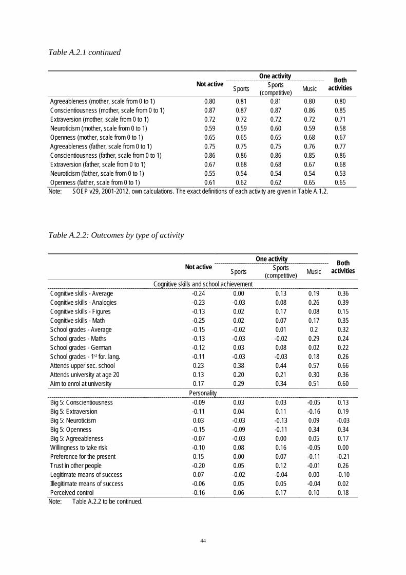
44

Table A.2.1 continued

Not active

One activity Both activities Sports Sports

(competitive) Music

Agreeableness (mother, scale from 0 to 1) 0.80 0.81 0.81 0.80 0.80 Conscientiousness (mother, scale from 0 to 1) 0.87 0.87 0.87 0.86 0.85 Extraversion (mother, scale from 0 to 1) 0.72 0.72 0.72 0.72 0.71 Neuroticism (mother, scale from 0 to 1) 0.59 0.59 0.60 0.59 0.58 Openness (mother, scale from 0 to 1) 0.65 0.65 0.65 0.68 0.67 Agreeableness (father, scale from 0 to 1) 0.75 0.75 0.75 0.76 0.77 Conscientiousness (father, scale from 0 to 1) 0.86 0.86 0.86 0.85 0.86 Extraversion (father, scale from 0 to 1) 0.67 0.68 0.68 0.67 0.68 Neuroticism (father, scale from 0 to 1) 0.55 0.54 0.54 0.54 0.53 Openness (father, scale from 0 to 1) 0.61 0.62 0.62 0.65 0.65

Note: SOEP v29, 2001-2012, own calculations. The exact definitions of each activity are given in Table A.1.2.

Table A.2.2: Outcomes by type of activity

Not active

One activity Both activities Sports Sports

(competitive) Music

Cognitive skills and school achievement Cognitive skills - Average -0.24 0.00 0.13 0.19 0.36 Cognitive skills - Analogies -0.23 -0.03 0.08 0.26 0.39 Cognitive skills - Figures -0.13 0.02 0.17 0.08 0.15 Cognitive skills - Math -0.25 0.02 0.07 0.17 0.35 School grades - Average -0.15 -0.02 0.01 0.2 0.32 School grades - Maths -0.13 -0.03 -0.02 0.29 0.24 School grades - German -0.12 0.03 0.08 0.02 0.22 School grades - 1st for. lang. -0.11 -0.03 -0.03 0.18 0.26 Attends upper sec. school 0.23 0.38 0.44 0.57 0.66 Attends university at age 20 0.13 0.20 0.21 0.30 0.36 Aim to enrol at university 0.17 0.29 0.34 0.51 0.60

Personality Big 5: Conscientiousness -0.09 0.03 0.03 -0.05 0.13 Big 5: Extraversion -0.11 0.04 0.11 -0.16 0.19 Big 5: Neuroticism 0.03 -0.03 -0.13 0.09 -0.03 Big 5: Openness -0.15 -0.09 -0.11 0.34 0.34 Big 5: Agreeableness -0.07 -0.03 0.00 0.05 0.17 Willingness to take risk -0.10 0.08 0.16 -0.05 0.00 Preference for the present 0.15 0.00 0.07 -0.11 -0.21 Trust in other people -0.20 0.05 0.12 -0.01 0.26 Legitimate means of success 0.07 -0.02 -0.04 0.00 -0.10 Illegitimate means of success -0.06 0.05 0.05 -0.04 0.02 Perceived control -0.16 0.06 0.17 0.10 0.18

Note: Table A.2.2 to be continued.

45

Table A.2.2 continued

Not active

One activity Both activities Sports Sports

(competitive) Music

Health and life style at age 20 Satisfaction with health 7.72 7.93 7.87 7.52 7.65 Current health situation 3.90 4.01 4.02 3.85 3.93 # of doctor visits 1.48 1.56 1.58 2.05 1.99 Currently smoking 0.40 0.32 0.29 0.25 0.21

Other leisure activities at age 17 Watching TV daily 0.81 0.80 0.79 0.69 0.67 Listening to music daily 0.88 0.88 0.88 0.88 0.91 Playing music weekly 0.12 0.16 0.15 0.83 0.80 Playing sports weekly 0.36 0.84 0.90 0.60 0.93 Playing theatre weekly 0.14 0.22 0.21 0.20 0.29 Reading daily 0.22 0.22 0.21 0.35 0.39 Voluntary engagement weekly 0.10 0.17 0.20 0.19 0.27 Hanging out daily 0.32 0.27 0.24 0.32 0.29 Surfing the internet daily 0.52 0.55 0.57 0.59 0.58 Going to church monthly 0.14 0.18 0.18 0.24 0.38 Playing computer games daily 0.26 0.30 0.31 0.200 0.21

Note: SOEP v29, 2001-2012, own calculations. The exact definitions of each activity are given in Table A.1.2. The exact measurement of all outcomes is described in Table E.1. School grades, cognitive skills and personality are nor-malised. All other outcome variables are binary, except for the following: Satisfaction with health (0 “worst” to 10 “best”), current health situation (1 “bad” to 5 “very good”) and # of doctor visits (number).

Table A.2.3: Characteristics of musical and athletic activities by gender

(1) (2) (3) (4)

Music only

Sports only (competitive and non-competitive)

Competitive sports only

Both: music and sports (competi-tive and non-competitive)

Music Sports Boys

Average starting age 9.3 8.8 8.2 9.1 9.0 Share doing sports/music in team (%) 60 73 86 56 65 Share with lessons/instructions (%) 76 64 81 77 67 Share playing sports/music daily (%) 50 32 39 44 39 Number of adolescents 135 973 577 220

Girls Average starting age 8.5 9.6 9.4 8.1 9.2 Share doing sports/music in team (%) 48 49 66 48 54 Share with lessons/instructions (%) 81 63 86 80 67 Share playing sports/music daily (%) 33 25 33 34 22 Number of adolescents 198 667 307 281

Note: SOEP v29, 2001-2012, own calculations. Column (3) is a subgroup of column (2), otherwise each column contains distinct individuals, who carry out either music (1), sports (2 with subgroup 3) or both (4). The exact definitions of sports and music participation are given in Table A.1.2.

46

Table A.2.4: Types of sports by gender (in % of all sports)

(1) (2) (3)

Sports

(competitive and non-competitive)

Sports (competitive)

Sports (in addition to music,

competitive and non-competitive) Boys

Basketball 5.3 3.8 4.1 Bicycling 5.3 0.7 7.7 Dancing (except ballet) 1.0 1.0 0.5 Equestrian sport 0.5 0.7 0.5 Fitness training 2.9 0.2 4.1 Handball 5.1 7.3 4.6 Jogging 1.7 1.2 3.6 Soccer 47.5 57.0 28.6 Swimming, diving 3.6 1.9 4.6 Volleyball 2.0 2.8 6.4

Girls Basketball 3.2 3.3 3.9 Bicycling 4.5 0.3 3.6 Dancing (except ballet) 12.1 11.8 16.8 Equestrian sport 12.5 11.2 14.3 Fitness training 1.2 0.0 0.4 Handball 5.4 10.8 5.0 Jogging 6.9 1.3 3.9 Soccer 7.4 12.1 4.6 Swimming, diving 7.5 3.6 6.1 Volleyball 9.2 10.8 10.0

Note: SOEP v29, 2001-2012, own calculations. The table shows the percentage of adolescents who state to play the type of sports defined in the first column among the group of adolescents defined in the column heading. The exact definitions of sports participation are given in Table A.1.2.

47

Appendix B: Further estimation results

B.1 Results of the estimation of the propensity score

Table B.1.1: Average marginal effects of the estimation of the propensity score

Music only vs.

Sport only

Music only vs.

Sport (competitive) only

Music and sport vs.

Sport only

Music and sport vs.

Music only (1) (2) (3) (4)

Marginal effects

p-value in %

Marginal effects

p-value in %

Marginal effects

p-value in %

Marginal effects

p-value in %

Constant -0.743 0 -0.531 0 -0.729 0 -0.187 40 Female (binary) 0.106 0 0.250 0 0.096 0 -0.035 31 Recommendation for upper sec-ondary school (binary)

0.044 2 0.089 0 0.148 0 0.141 0

Difference: birth year - 1981 0.007 1 0.006 14 0.006 3 0.000 94 Birth year 1982 or 1983 (binary) 0.053 22 0.006 91 -0.053 17 -0.138 13 Birth order -0.033 1 -0.043 2 -0.040 0 0.004 88 Single parent household (binary) -0.007 78 0.005 89 0.018 50 0.021 71 Number of siblings in SOEP 0.023 1 0.030 2 0.032 0 0.011 50 Household lives in rural area (binary)

0.039 9 0.058 8 0.011 65 -0.055 23

North West Germany (binary) -0.056 1 -0.105 0 -0.051 4 0.056 30 North Rhine Westphalia (binary) -0.058 1 -0.100 0 -0.092 0 -0.020 72 Hesse (binary) -0.058 4 -0.064 19 -0.060 5 0.041 55 Berlin and Brandenburg (binary) -0.031 45 -0.044 51 -0.095 0 -0.094 37 Saxony (binary) 0.070 11 0.133 1 0.074 9 -0.047 51 South East Germany (binary) 0.008 82 -0.075 14 -0.089 1 -0.166 5 City states: Bremen, Hamburg, Berlin (binary)

0.083 17 0.239 0 0.141 2 -0.003 98

Household net overall wealth (in 100,000 euros)

0.001 80 -0.002 47 0.001 73 0.000 100

Log of labour market income (both parents)

-0.001 89 0.012 28 0.005 59 0.017 35

Age of mother at birth 0.005 3 0.011 0 0.009 0 0.004 42 Hours working (mother) -0.001 19 -0.002 5 -0.002 1 -0.001 60 Hours working (father) 0.001 13 0.002 12 0.002 4 0.001 70 Mother working in services (binary)

0.073 1 0.056 17 0.056 6 -0.051 38

Father working in services (binary)

-0.005 88 -0.028 58 -0.019 60 -0.044 52

Mother working in manufacturing or agriculture (binary)

0.120 1 0.138 2 0.077 9 -0.056 48

Father working in manufacturing or agriculture (binary)

-0.020 55 -0.072 15 -0.041 25 -0.061 37

ISEI socio-economic status (high-est among parents, scale from 0 to 90)

0.001 51 0.000 85 0.001 31 0.001 70

Mother’s job requires no training (binary)

-0.033 15 0.008 83 -0.008 76 0.036 47

Father’s job requires no training (binary)

-0.014 62 -0.062 13 -0.042 17 -0.021 77

Note: Table B.1.1 to be continued.

48

Table B.1.1 continued

Music only vs.

Sport only

Music only vs.

Sport (competitive) only

Music and sport vs.

Sport only

Music and sport vs.

Music only (1) (2) (3) (4)

Marginal effects

p-value in %

Marginal effects

p-value in %

Marginal effects

p-value in %

Marginal effects

p-value in %

Mother’s willingness to take risks (scale from 0 to 10)

-0.008 7 -0.015 3 -0.008 8 0.005 61

Father’s willingness to take risks (scale from 0 to 10)

-0.011 1 -0.015 2 -0.011 1 0.002 80

Missing: mother’s willingness to take risks (binary)

0.107 3 0.132 2 0.080 10 -0.046 58

Missing: father’s willingness to take risks (binary)

-0.056 6 -0.118 1 -0.045 18 0.016 82

At least one parent with university degree (binary)

0.004 90 0.012 76 0.048 9 0.035 55

At least one parent with vocational degree (binary)

-0.021 38 -0.003 92 0.035 12 0.061 20

At least one parent with upper secondary school degree (binary)

0.039 14 0.050 18 0.033 21 -0.038 47

At least one parent with migration background (binary)

-0.023 34 0.015 68 0.027 31 0.078 12

Agreeableness (mother, scale from 0 to 1)

-0.162 3 -0.288 1 -0.129 10 0.130 42

Conscientiousness (mother, scale from 0 to 1)

0.010 91 -0.041 76 -0.092 31 -0.243 17

Extraversion (mother, scale from 0 to 1)

-0.081 22 -0.152 12 -0.088 21 -0.041 77

Neuroticism (mother, scale from 0 to 1)

-0.025 66 -0.106 21 -0.042 48 -0.058 61

Openness (mother, scale from 0 to 1)

0.142 3 0.227 2 0.120 8 -0.065 63

Agreeableness (father, scale from 0 to 1)

0.079 32 0.184 12 0.124 11 0.054 73

Conscientiousness (father, scale from 0 to 1)

0.048 57 0.120 37 0.120 18 0.179 37

Extraversion (father, scale from 0 to 1)

-0.072 30 -0.075 46 -0.077 29 0.059 68

Neuroticism (father, scale from 0 to 1)

0.157 1 0.099 28 0.087 17 -0.099 45

Openness (father, scale from 0 to 1)

0.141 5 0.243 2 0.172 2 -0.034 82

Efron’s R Square 0.111 0.186 0.160 0.069 Number of observations 1973 1463 2141 834 Note: SOEP v29, 2001-2012, own calculations. The exact definitions of each activity are given in Table 3.2. Inference

based on 4999 bootstrap replications. Numbers in italics / bold / bold italics indicate significance at the 10%/5%/1% level.

49

Table B.1.2: Balancing of covariates after matching

Music only vs.

Sport only

Music only vs.

Sport (competitive) only

Music and sport vs.

Sport only

Music and sport vs.

Music only (1) (2) (3) (4)

Std. bias in %

p-value in %

Std. bias in %

p-value in %

Std. bias in %

p-value in %

Std. bias in %

p-value in %

Female (binary) 0.0 100 0.0 100 0.0 100 0.0 100 Recommendation for upper secondary school (binary) -0.8 80 -2.5 40 -1.7 59 -1.7 59 Difference: birth year - 1981 -2.9 33 3.3 27 0.4 89 0.5 87 Birth year 1982 or 1983 (binary) -0.1 98 -1.0 75 -1.0 76 -1.0 76 Birth order 1.3 67 0.8 78 -1.0 74 -1.1 73 Single parent household (binary) -0.2 96 1.1 71 0.9 77 0.9 77 Number of siblings in SOEP 1.5 62 0.5 87 -0.8 80 -0.8 80 Household lives in rural area (binary) -0.6 83 1.7 58 0.9 76 1.0 75 North West Germany (binary) -0.9 77 1.2 70 1.5 63 1.5 63 North Rhine Westphalia (binary) -4.5 13 -1.4 65 -1.8 56 -1.8 56 Hesse (binary) 1.2 70 0.8 78 -0.4 91 -0.4 91 Berlin and Brandenburg (binary) 0.5 85 -0.7 80 0.0 99 0.0 99 Saxony (binary) 0.0 100 1.4 63 0.2 94 0.2 94 South East Germany (binary) -0.1 96 -0.5 87 -2.2 49 -2.2 49 City states: Bremen, Hamburg, Berlin (binary) 1.4 65 1.1 72 -0.2 96 -0.2 96 Household net overall wealth (in 100,000 euros) 1.2 69 0.2 96 -1.0 74 -1.1 73 Log of labour market income (both parents) -2.9 33 -2.0 50 -5.5 8 -5.5 8 Age of mother at birth 1.8 54 1.4 64 1.3 69 1.3 68 Hours working (mother) -0.7 82 -1.2 69 -2.9 36 -2.8 37 Hours working (father) 0.3 91 0.9 77 -0.4 91 -0.4 90 Mother working in services (binary) -1.0 74 -0.9 76 -0.5 87 -0.4 89 Father working in services (binary) -1.6 59 -0.4 89 -1.8 57 -1.8 56 Mother working in manufacturing or agriculture (binary) 0.6 85 0.3 93 -1.8 56 -1.8 56 Father working in manufacturing or agriculture (binary) 1.6 60 0.6 83 -0.7 83 -0.6 84 ISEI socio-economic status (highest among parents, scale from 0 to 90) -1.4 63 -2.3 44 -4.4 16 -4.4 15 Mother’s job requires no training (binary) 1.5 62 0.1 98 -4.7 13 -4.7 13 Father’s job requires no training (binary) -1.2 69 -1.6 59 -1.7 58 -1.7 58 Mother’s willingness to take risks (scale from 0 to 10) -0.7 82 -0.8 78 -4.2 18 -4.1 19 Father’s willingness to take risks (scale from 0 to 10) 1.6 58 2.1 48 -1.6 61 -1.6 60 Note: Table B.1.2 to be continued.

50

Table B.1.2 continued

Music only vs.

Sport only

Music only vs.

Sport (competitive) only

Music and sport vs.

Sport only

Music and sport vs.

Music only (1) (2) (3) (4)

Std. bias in %

p-value in %

Std. bias in %

p-value in %

Std. bias in %

p-value in %

Std. bias in %

p-value in %

Missing: mother’s willingness to take risks (binary) 0.7 82 1.6 60 -1.6 62 -1.6 61 Missing: father’s willingness to take risks (binary) -0.6 83 2.3 43 2.3 46 2.3 46 At least one parent with university degree (binary) -1.0 73 -0.4 90 -1.3 68 -1.3 68 At least one parent with vocational degree (binary) 1.1 71 -0.8 79 -0.1 97 -0.2 95 At least one parent with upper secondary school degree (binary) -2.0 51 -1.5 62 -1.9 55 -1.9 55 At least one parent with migration background (binary) -2.1 49 0.1 97 2.5 43 2.5 43 Agreeableness (mother, scale from 0 to 1) -1.8 54 -1.8 54 -0.9 78 -0.9 77 Conscientiousness (mother, scale from 0 to 1) -1.4 64 -2.0 51 0.6 84 0.6 85 Extraversion (mother, scale from 0 to 1) -2.1 48 -2.3 43 -3.1 32 -3.1 33 Neuroticism (mother, scale from 0 to 1) 0.2 94 1.6 59 0.8 79 0.8 79 Openness (mother, scale from 0 to 1) -1.5 63 -0.9 75 0.4 89 0.4 89 Agreeableness (father, scale from 0 to 1) -2.5 41 -1.1 71 -3.7 23 -3.8 23 Conscientiousness (father, scale from 0 to 1) -1.3 67 -2.4 42 -1.1 72 -1.1 73 Extraversion (father, scale from 0 to 1) 0.5 86 -1.6 59 0.3 93 0.1 97 Neuroticism (father, scale from 0 to 1) -0.3 93 -1.3 67 1.1 73 1.1 72 Openness (father, scale from 0 to 1) -0.2 93 -1.1 72 -0.2 95 -0.2 94 Note: SOEP v29, 2001-2012, own calculations. The table indicates the standard bias (including the p-value) between

treatment and control group after matching when estimating the Average Treatment Effect on the Treated (ATET). The biases for the estimation of the Average Treatment Effect on the Non-treatet (ATENT) are not significant for any of the covariates either and can be provided by the authors on request. The exact definitions of each activity are given in Table 3.2. Inference based on 4999 bootstrap replications. Numbers in italics / bold / bold italics indi-cate significance at the 10%/5%/1% level.

51

B.2 Full set of effects

Table B.2.1: Average effects of music vs. sports

Music only vs.

Sport only

Music only vs.

Sport (competitive) only

Music and sport vs.

Sport only

Music and sport vs.

Music only (1) (2) (3) (4)

Outcome variables Effect p-value in %

Effect p-value in %

Effect p-value in %

Effect p-value in %

Cognitive skills and school achievement at age 17 Cognitive skills - Average 0.012 90 0.073 48 0.233 1 0.230 5 Cognitive skills - Analogies 0.054 58 0.143 17 0.216 1 0.169 15 Cognitive skills - Figures 0.053 59 0.108 26 0.276 0 0.229 5 Cognitive skills - Math -0.045 63 -0.065 51 0.070 45 0.123 30 School grades – Average 0.034 66 0.091 19 0.151 3 0.123 20 School grades - Maths -0.119 14 -0.075 30 0.113 12 0.233 2 School grades - German 0.172 2 0.196 0 0.113 11 -0.051 59 School grades - 1st for. lang. 0.063 42 0.130 6 0.103 13 0.046 63 Attends upper sec. school 0.081 4 0.083 2 0.135 0 0.063 18 Aim to enrol at university 0.106 1 0.115 0 0.187 0 0.087 6 Attends university at age 20 0.024 48 0.085 2 0.084 1 0.065 13

Personality at age 17 Big 5: Conscientiousness -0.114 21 -0.053 60 0.059 51 0.165 14 Big 5: Extraversion -0.165 9 -0.171 8 0.128 13 0.294 1 Big 5: Neuroticism 0.103 31 0.104 26 0.013 88 -0.090 47 Big 5: Openness 0.407 0 0.348 0 0.349 0 -0.058 63 Big 5: Agreeableness 0.048 60 0.032 73 0.206 2 0.152 17 Willingness to take risk -0.211 4 -0.239 1 -0.181 6 0.021 87 Preference for the present -0.155 9 -0.150 11 -0.092 35 0.062 61 Trust in other people 0.016 88 -0.051 62 0.211 1 0.194 10 Legitimate means of success 0.042 54 -0.019 76 -0.045 50 -0.082 35 Illegitimate means of success 0.046 51 -0.099 14 -0.074 30 -0.118 20 Perceived control 0.109 13 -0.069 29 0.099 14 -0.007 93

Health and life style at age 18 Satisfaction with health -0.119 45 -0.341 2 -0.143 28 -0.050 80 Current health situation -0.138 4 -0.195 0 -0.048 39 0.083 30 # of doctor visits 0.403 44 0.769 7 0.081 72 -0.291 59 Currently smoking -0.007 88 0.008 83 -0.110 0 -0.107 5

Other leisure activities at age 17 Watching TV daily -0.099 0 -0.080 1 -0.115 0 -0.016 71 Listening to music daily 0.011 66 0.015 45 0.020 36 0.009 75 Playing theatre weekly -0.053 4 -0.004 88 0.007 79 0.063 6 Reading daily 0.067 5 0.134 0 0.127 0 0.062 14 Voluntary engagement weekly -0.018 53 0.023 41 0.068 2 0.089 1 Hanging out daily -0.005 88 0.059 7 0.024 46 0.034 42 Surfing the internet daily 0.067 17 -0.026 58 0.033 47 -0.034 56 Going to church monthly 0.040 33 0.049 23 0.169 0 0.126 2 Playing computer games daily -0.075 2 -0.099 0 -0.044 14 0.029 47 Note: Effects presented are average treatment effects for the target population. Inference is based on 4999 bootstrap

replications. Numbers in italics / bold / bold italics indicate significance at the 10% / 5% / 1% level. The measure-ment of all outcomes is described in Table E.1. School grades, cognitive skills and personality are normalised to mean zero and variance 1 (higher value of grades is better). All other outcome variables are binary, except for the following: Satisfaction with health (0 “Worst” to 10 “Best”), current health situation (1 “Bad” to 5 “Very good”) and # of doctor visits (number).

52

B.3 Heterogeneity of the effects

Table B.3.1: Average effects of music vs. sports (female adolescents)

Music only vs.

Sport only

Music only vs.

Sport (competitive) only

Music and sport vs.

Sport only

Music and sport vs.

Music only (1) (2) (3) (4)

Outcome variables Effect p-value in %

Effect p-value in %

Effect p-value in %

Effect p-value in %

Cognitive skills and school achievement at age 17 Cognitive skills - Average 0.250 5 -0.018 89 -0.042 73 -0.282 5 Cognitive skills - Analogies 0.267 3 0.150 27 0.076 48 -0.184 18 Cognitive skills - Figures 0.210 14 -0.067 63 -0.021 86 -0.220 15 Cognitive skills - Math 0.139 26 -0.056 68 -0.120 39 -0.255 9 School grades – Average 0.103 28 -0.145 42 0.087 27 -0.011 91 School grades - Maths 0.003 96 -0.233 10 -0.028 76 -0.029 84 School grades - German 0.248 2 0.043 62 0.102 24 -0.139 22 School grades - 1st for. lang. 0.017 84 -0.110 59 0.108 19 0.094 41 Attends upper sec. school 0.073 12 0.014 75 0.014 76 -0.055 41 Attends university at age 20 0.036 50 0.027 55 0.041 41 0.007 92 Aim to enrol at university 0.054 26 0.038 41 0.057 18 0.006 89

Personality at age 17 Big 5: Conscientiousness 0.001 96 -0.162 28 0.110 29 0.108 49 Big 5: Extraversion -0.049 70 -0.053 76 0.029 79 0.081 61 Big 5: Neuroticism -0.024 86 0.193 25 0.124 46 0.150 43 Big 5: Openness 0.468 0 0.251 8 0.105 44 -0.359 13 Big 5: Agreeableness 0.093 52 -0.014 90 0.188 13 0.092 56 Willingness to take risk -0.004 96 -0.143 27 -0.078 47 -0.071 61 Preference for the present -0.265 11 -0.188 17 -0.162 17 0.100 59 Trust in other people 0.088 57 -0.043 79 0.164 20 0.076 69 Legitimate means of success -0.014 91 -0.075 63 -0.046 53 -0.030 81 Illegitimate means of success -0.223 2 -0.278 0 -0.134 15 0.092 42 Perceived control 0.037 81 -0.405 0 -0.108 25 -0.141 32

Health and life style at age 18 Satisfaction with health -0.070 75 -0.178 31 -0.204 29 -0.130 63 Current health situation -0.047 71 -0.073 37 -0.115 17 -0.061 69 # of doctor visits 0.232 47 0.181 72 0.271 33 0.042 89 Currently smoking -0.066 14 0.001 96 -0.023 63 0.042 50

Other leisure activities at age 17 Watching TV daily -0.065 13 -0.026 52 -0.009 75 0.055 25 Listening to music daily -0.012 73 0.005 84 0.041 16 0.053 12 Playing theatre weekly -0.057 19 0.012 78 0.074 11 0.132 2 Reading daily 0.149 0 0.132 0 0.132 0 -0.016 78 Voluntary engagement weekly 0.026 47 0.073 5 0.083 4 0.059 20 Hanging out daily 0.049 29 0.121 1 -0.026 56 -0.072 17 Surfing the internet daily -0.037 65 -0.094 20 -0.119 5 -0.079 33 Going to church monthly 0.025 69 0.124 6 0.191 0 0.166 2 Playing computer games daily -0.028 32 -0.009 74 -0.027 44 0.001 96 Note: Effects presented are average treatment effects for the target population. Inference is based on 499 bootstrap

replications. Numbers in italics / bold / bold italics indicate significance at the 10% / 5% / 1% level. The measure-ment of all outcomes is described in Table E.1. School grades, cognitive skills and personality are normalised. All other outcome variables are binary, except for the following: Satisfaction with health (0 “Worst” to 10 “Best”), cur-rent health situation (1 “Bad” to 5 “Very good”) and # of doctor visits (number).

53

Table B.3.2: Average effects of music vs. sports (male adolescents)

Music only vs.

Sport only

Music only vs.

Sport (competitive) only

Music and sport vs.

Sport only

Music and sport vs.

Music only (1) (2) (3) (4)

Outcome variables Effect p-value in %

Effect p-value in %

Effect p-value in %

Effect p-value in %

Cognitive skills and school achievement at age 17 Cognitive skills - Average -0.246 15 -0.001 97 0.216 42 0.467 20 Cognitive skills - Analogies -0.119 57 0.141 33 0.315 21 0.436 24 Cognitive skills - Figures -0.204 28 -0.007 95 0.055 82 0.265 40 Cognitive skills - Math -0.235 8 -0.125 54 0.043 87 0.282 35 School grades – Average -0.109 41 -0.017 89 0.208 19 0.319 14 School grades - Maths -0.234 8 -0.117 27 0.123 31 0.357 6 School grades - German 0.146 25 0.066 61 0.144 43 0.001 97 School grades - 1st for. lang. -0.205 36 0.015 90 0.191 22 0.397 17 Attends upper sec. school 0.048 55 0.012 85 0.138 2 0.093 36 Attends university at age 20 0.048 38 0.081 8 0.186 5 0.138 15 Aim to enrol at university 0.122 7 0.121 1 0.172 1 0.051 59

Personality at age 17 Big 5: Conscientiousness -0.167 29 -0.233 26 0.068 67 0.235 30 Big 5: Extraversion -0.310 7 -0.283 4 0.108 53 0.421 4 Big 5: Neuroticism 0.138 48 0.106 41 0.056 72 -0.084 72 Big 5: Openness 0.480 0 0.482 0 0.481 0 0.003 97 Big 5: Agreeableness 0.072 65 -0.076 61 0.066 56 -0.005 95 Willingness to take risk -0.304 13 -0.171 28 -0.174 54 0.135 58 Preference for the present 0.184 54 -0.133 43 -0.194 17 -0.379 23 Trust in other people -0.076 64 -0.053 71 0.021 93 0.098 70 Legitimate means of success 0.109 60 -0.042 68 -0.042 82 -0.153 47 Illegitimate means of success -0.080 51 -0.054 62 -0.133 38 -0.054 76 Perceived control 0.105 42 0.065 53 0.043 84 -0.057 76

Health and life style at age 18 Satisfaction with health 0.139 46 -0.015 90 -0.291 51 -0.428 29 Current health situation -0.073 42 -0.055 46 -0.102 45 -0.029 88 # of doctor visits -0.134 77 -0.187 54 0.307 54 0.431 50 Currently smoking -0.073 55 -0.008 93 -0.106 7 -0.033 80

Other leisure activities at age 17 Watching TV daily 0.003 95 -0.044 31 -0.162 1 -0.166 5 Listening to music daily 0.063 0 0.035 18 0.052 17 -0.011 73 Playing theatre weekly -0.035 41 0.010 84 0.067 33 0.102 16 Reading daily 0.045 40 0.050 42 0.101 9 0.056 47 Voluntary engagement weekly -0.077 5 -0.035 32 0.076 17 0.153 2 Hanging out daily 0.017 84 0.044 34 -0.008 90 -0.024 84 Surfing the internet daily 0.153 9 0.038 60 0.176 1 0.025 78 Going to church monthly -0.001 96 0.027 61 0.131 8 0.134 16 Playing computer games daily 0.050 76 0.002 95 -0.083 17 -0.133 39 Note: Effects presented are average treatment effects for the target population.). Inference is based on 499 bootstrap

replications. Numbers in italics / bold / bold italics indicate significance at the 10% / 5% / 1% level. The measure-ment of all outcomes is described in Table E.1. School grades, cognitive skills and personality are normalised. All other outcome variables are binary, except for the following: Satisfaction with health (0 “Worst” to 10 “Best”), cur-rent health situation (1 “Bad” to 5 “Very good”) and # of doctor visits (number).

54

Table B.3.3: Average effects of music vs. sports (adolescents without recommendation for

upper secondary school at the end of primary school)

Music only vs.

Sport only

Music only vs.

Sport (competitive) only

Music and sport vs.

Sport only

Music and sport vs.

Music only (1) (2) (3) (4)

Outcome variables Effect p-value in %

Effect p-value in %

Effect p-value in %

Effect p-value in %

Cognitive skills and school achievement at age 17 Cognitive skills - Average 0.120 57 -0.032 89 -0.170 43 -0.292 31 Cognitive skills - Analogies 0.137 51 0.186 41 -0.021 89 -0.161 53 Cognitive skills - Figures 0.058 74 0.022 92 -0.258 36 -0.320 28 Cognitive skills - Math 0.100 59 -0.235 9 -0.172 46 -0.271 39 School grades – Average -0.051 65 -0.005 95 0.035 78 0.093 53 School grades - Maths -0.194 13 -0.235 3 -0.131 32 0.068 66 School grades - German 0.180 8 0.156 12 0.038 74 -0.138 29 School grades - 1st for. lang. -0.076 59 0.088 44 0.139 26 0.218 22 Attends upper sec. school 0.032 49 0.017 67 0.045 35 0.014 81 Attends university at age 20 0.015 76 0.034 42 0.056 29 0.044 45 Aim to enrol at university 0.012 80 0.023 54 0.081 9 0.069 27

Personality at age 17 Big 5: Conscientiousness -0.222 27 -0.407 24 -0.059 65 0.141 52 Big 5: Extraversion -0.230 24 -0.405 1 0.100 41 0.340 15 Big 5: Neuroticism 0.160 50 0.028 86 -0.187 26 -0.367 21 Big 5: Openness 0.191 22 0.156 34 0.235 4 0.019 91 Big 5: Agreeableness 0.049 82 0.033 85 -0.069 70 -0.127 57 Willingness to take risk -0.091 67 -0.092 54 -0.080 66 0.009 96 Preference for the present 0.214 24 0.135 67 -0.152 33 -0.358 17 Trust in other people -0.015 95 0.078 71 0.222 10 0.225 42 Legitimate means of success 0.038 71 0.023 85 -0.247 7 -0.279 9 Illegitimate means of success 0.074 51 0.008 94 -0.124 39 -0.197 35 Perceived control -0.045 74 -0.157 16 -0.028 85 0.026 90

Health and life style at age 18 Satisfaction with health -0.288 40 -0.210 28 -0.261 44 0.019 94 Current health situation -0.121 20 -0.183 6 -0.078 43 0.041 76 # of doctor visits 0.358 76 -0.351 44 0.006 96 -0.363 75 Currently smoking -0.022 81 -0.042 49 -0.147 3 -0.126 25

Other leisure activities at age 17 Watching TV daily 0.017 69 -0.005 89 -0.026 62 -0.044 40 Listening to music daily 0.027 33 0.015 55 0.073 2 0.045 17 Playing theatre weekly -0.084 5 -0.071 7 0.078 40 0.163 3 Reading daily 0.025 58 0.126 0 0.068 23 0.044 54 Voluntary engagement weekly -0.054 12 -0.007 85 0.127 13 0.182 3 Hanging out daily 0.011 82 0.147 1 0.105 6 0.096 25 Surfing the internet daily 0.135 17 0.070 37 -0.023 74 -0.157 17 Going to church monthly -0.094 1 -0.002 95 0.196 0 0.286 0 Playing computer games daily 0.054 34 0.031 53 -0.007 90 -0.063 47 Note: Effects presented are average treatment effects for target population (.). Inference based on 499 bootstrap replica-

tions. Numbers in italics / bold / bold italics indicate significance at the 10% / 5% / 1% level. The measurement of all outcomes is described in Table E.1. School grades, cognitive skills and personality are normalised. All other outcome variables are binary, except for the following: Satisfaction with health (0 “Worst” to 10 “Best”), current health situation (1 “Bad” to 5 “Very good”) and # of doctor visits (number).

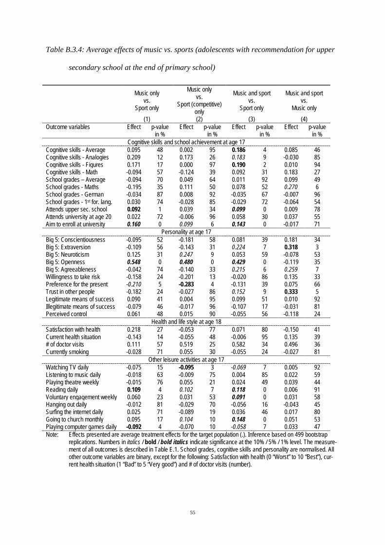
55

Table B.3.4: Average effects of music vs. sports (adolescents with recommendation for upper

secondary school at the end of primary school)

Music only vs.

Sport only

Music only vs.

Sport (competitive) only

Music and sport vs.

Sport only

Music and sport vs.

Music only (1) (2) (3) (4)

Outcome variables Effect p-value in %

Effect p-value in %

Effect p-value in %

Effect p-value in %

Cognitive skills and school achievement at age 17 Cognitive skills - Average 0.095 48 0.002 95 0.186 4 0.085 46 Cognitive skills - Analogies 0.209 12 0.173 26 0.183 9 -0.030 85 Cognitive skills - Figures 0.171 17 0.000 97 0.190 2 0.010 94 Cognitive skills - Math -0.094 57 -0.124 39 0.092 31 0.183 27 School grades – Average -0.094 70 0.049 64 0.011 92 0.099 49 School grades - Maths -0.195 35 0.111 50 0.078 52 0.270 6 School grades - German -0.034 87 0.008 92 -0.035 67 -0.007 96 School grades - 1st for. lang. 0.030 74 -0.028 85 -0.029 72 -0.064 54 Attends upper sec. school 0.092 1 0.039 34 0.099 0 0.009 78 Attends university at age 20 0.022 72 -0.006 96 0.058 30 0.037 55 Aim to enroll at university 0.160 0 0.099 6 0.143 0 -0.017 71

Personality at age 17 Big 5: Conscientiousness -0.095 52 -0.181 58 0.081 39 0.181 34 Big 5: Extraversion -0.109 56 -0.143 31 0.224 7 0.318 3 Big 5: Neuroticism 0.125 31 0.247 9 0.053 59 -0.078 53 Big 5: Openness 0.548 0 0.480 0 0.429 0 -0.119 35 Big 5: Agreeableness -0.042 74 -0.140 33 0.215 6 0.259 7 Willingness to take risk -0.158 24 -0.201 13 -0.020 86 0.135 33 Preference for the present -0.210 5 -0.283 4 -0.131 39 0.075 66 Trust in other people -0.182 24 -0.027 86 0.152 9 0.333 5 Legitimate means of success 0.090 41 0.004 95 0.099 51 0.010 92 Illegitimate means of success -0.079 46 -0.017 96 -0.107 17 -0.031 81 Perceived control 0.061 48 0.015 90 -0.055 56 -0.118 24

Health and life style at age 18 Satisfaction with health 0.218 27 -0.053 77 0.071 80 -0.150 41 Current health situation -0.143 14 -0.055 48 -0.006 95 0.135 39 # of doctor visits 0.111 57 0.519 25 0.582 34 0.496 36 Currently smoking -0.028 71 0.055 30 -0.055 24 -0.027 81

Other leisure activities at age 17 Watching TV daily -0.075 15 -0.095 3 -0.069 7 0.005 92 Listening to music daily -0.018 63 -0.009 75 0.004 85 0.022 59 Playing theatre weekly -0.015 76 0.055 21 0.024 49 0.039 44 Reading daily 0.109 4 0.102 7 0.118 0 0.006 91 Voluntary engagement weekly 0.060 23 0.031 53 0.091 0 0.031 58 Hanging out daily -0.012 81 -0.029 70 -0.056 16 -0.043 45 Surfing the internet daily 0.025 71 -0.089 19 0.036 46 0.017 80 Going to church monthly 0.095 17 0.104 10 0.148 0 0.051 53 Playing computer games daily -0.092 4 -0.070 10 -0.058 7 0.033 47 Note: Effects presented are average treatment effects for the target population (.). Inference based on 499 bootstrap

replications. Numbers in italics / bold / bold italics indicate significance at the 10% / 5% / 1% level. The measure-ment of all outcomes is described in Table E.1. School grades, cognitive skills and personality are normalised. All other outcome variables are binary, except for the following: Satisfaction with health (0 “Worst” to 10 “Best”), cur-rent health situation (1 “Bad” to 5 “Very good”) and # of doctor visits (number).

56

Table B.3.5: Average effects of music vs. sports (adolescents with parents who did not receive

an upper secondary school degree)

Music only vs.

Sport only

Music only vs.

Sport (competitive) only

Music and sport vs.

Sport only

Music and sport vs.

Music only (1) (2) (3) (4)

Outcome variables Effect p-value in %

Effect p-value in %

Effect p-value in %

Effect p-value in %

Cognitive skills and school achievement at age 17 Cognitive skills - Average 0.099 43 0.050 68 -0.062 79 -0.160 47 Cognitive skills - Analogies 0.087 52 0.101 46 0.030 85 -0.054 77 Cognitive skills - Figures 0.134 26 0.021 87 -0.070 78 -0.203 33 Cognitive skills - Math 0.039 78 -0.019 89 -0.203 36 -0.242 30 School grades – Average 0.034 78 -0.035 75 -0.057 60 -0.091 52 School grades - Maths -0.051 67 -0.103 30 0.012 91 0.070 69 School grades - German 0.075 55 0.007 94 -0.145 34 -0.221 11 School grades - 1st for. lang. 0.044 76 -0.055 60 -0.047 68 -0.099 56 Attends upper sec. school 0.067 25 0.017 71 0.138 3 0.075 53 Attends university at age 20 -0.017 73 0.053 13 0.051 44 0.069 27 Aim to enrol at university 0.065 23 0.041 33 0.065 25 0.006 92

Personality at age 17 Big 5: Conscientiousness -0.123 32 -0.028 86 -0.097 59 0.024 91 Big 5: Extraversion -0.260 5 -0.111 40 0.277 4 0.535 0 Big 5: Neuroticism 0.235 12 0.228 7 -0.092 49 -0.327 11 Big 5: Openness 0.337 2 0.419 0 0.207 18 -0.130 51 Big 5: Agreeableness 0.172 27 0.115 35 0.085 39 -0.083 64 Willingness to take risk -0.355 4 -0.103 52 0.127 22 0.481 3 Preference for the present -0.148 27 -0.242 13 -0.156 16 -0.011 94 Trust in other people -0.127 34 -0.116 32 0.274 11 0.407 7 Legitimate means of success -0.029 88 -0.029 73 -0.198 12 -0.166 26 Illegitimate means of success -0.124 24 -0.141 13 -0.174 42 -0.047 81 Perceived control 0.017 91 -0.148 14 0.097 37 0.075 66

Health and life style at age 18 Satisfaction with health 0.115 56 -0.176 29 -0.430 37 -0.553 30 Current health situation -0.128 9 -0.151 9 -0.040 66 0.089 41 # of doctor visits -0.015 95 0.252 50 0.420 31 0.462 42 Currently smoking 0.033 84 0.008 90 -0.106 13 -0.139 41

Other leisure activities at age 17 Watching TV daily -0.060 25 -0.056 17 -0.022 68 0.036 60 Listening to music daily -0.017 74 0.033 22 0.078 0 0.095 8 Playing theatre weekly -0.071 23 -0.023 48 -0.020 69 0.051 53 Reading daily 0.078 18 0.102 3 0.060 24 -0.022 77 Voluntary engagement weekly -0.034 31 0.016 60 0.129 10 0.164 4 Hanging out daily -0.029 68 0.127 1 0.021 71 0.050 52 Surfing the internet daily 0.062 38 0.017 81 0.091 23 0.030 73 Going to church monthly 0.097 22 0.107 12 0.209 2 0.111 20 Playing computer games daily -0.051 41 -0.024 58 0.011 92 0.065 51 Note: Effects presented are average treatment effects for the target population (.). P-values are based on 499 bootstrap

replications. Numbers in italics / bold / bold italics indicate significance at the 10% / 5% / 1% level. The measure-ment of all outcomes is described in Table E.1. School grades, cognitive skills and personality are normalised. All other outcome variables are binary, except for the following: Satisfaction with health (0 “Worst” to 10 “Best”), cur-rent health situation (1 “Bad” to 5 “Very good”) and # of doctor visits (number).

57

Table B.3.6: Average effects of music vs. sports (adolescents with parents who have an upper

secondary school degree)

Music only vs.

Sport only

Music only vs.

Sport (competitive) only

Music and sport vs.

Sport only

Music and sport vs.

Music only (1) (2) (3) (4)

Outcome variables Effect p-value in %

Effect p-value in %

Effect p-value in %

Effect p-value in %

Cognitive skills and school achievement at age 17 Cognitive skills - Average -0.103 45 -0.146 34 0.136 31 0.235 14 Cognitive skills - Analogies -0.018 86 -0.004 95 0.093 56 0.107 50 Cognitive skills - Figures -0.156 25 -0.169 24 0.073 53 0.233 15 Cognitive skills - Math -0.068 65 -0.148 37 0.146 39 0.207 20 School grades – Average -0.055 53 0.029 77 0.026 89 0.079 59 School grades - Maths -0.194 5 -0.098 33 -0.036 82 0.156 33 School grades - German 0.049 69 0.029 81 -0.013 95 -0.063 61 School grades - 1st for. lang. 0.051 57 0.149 13 0.126 26 0.072 59 Attends upper sec. school 0.074 8 -0.018 72 0.029 55 -0.045 51 Attends university at age 20 0.080 21 -0.033 79 0.036 56 -0.042 63 Aim to enrol at university 0.113 1 0.078 13 0.078 16 -0.036 58

Personality at age 17 Big 5: Conscientiousness -0.069 63 0.066 65 0.016 89 0.081 63 Big 5: Extraversion -0.254 18 -0.098 55 0.044 80 0.294 16 Big 5: Neuroticism 0.035 86 -0.068 73 0.013 93 -0.014 93 Big 5: Openness 0.322 7 0.334 0 0.350 0 0.027 90 Big 5: Agreeableness -0.073 60 -0.072 53 0.169 41 0.236 25 Willingness to take risk -0.089 55 -0.063 84 -0.276 6 -0.185 28 Preference for the present -0.045 73 -0.045 79 -0.049 79 -0.005 95 Trust in other people 0.168 26 -0.087 59 0.138 33 -0.036 85 Legitimate means of success -0.093 45 -0.028 75 -0.127 33 -0.031 77 Illegitimate means of success -0.086 45 -0.110 35 -0.098 22 -0.012 91 Perceived control 0.061 58 -0.045 71 -0.030 72 -0.090 53

Health and life style at age 18 Satisfaction with health -0.253 27 -0.004 97 0.058 77 0.312 27 Current health situation -0.196 5 -0.035 75 -0.129 11 0.070 52 # of doctor visits 0.024 93 -0.100 73 -0.126 46 -0.148 53 Currently smoking -0.086 10 -0.023 61 -0.094 10 -0.008 89

Other leisure activities at age 17 Watching TV daily -0.014 83 -0.020 72 -0.028 71 -0.015 78 Listening to music daily -0.022 69 0.015 61 0.013 56 0.035 43 Playing theatre weekly 0.015 79 0.050 25 0.003 95 -0.011 85 Reading daily 0.094 8 0.123 1 0.117 1 0.023 72 Voluntary engagement weekly -0.033 56 -0.036 45 0.048 32 0.079 21 Hanging out daily -0.031 56 0.064 12 -0.021 59 0.009 88 Surfing the internet daily 0.059 41 0.052 54 -0.011 86 -0.071 33 Going to church monthly -0.019 80 0.026 75 0.101 39 0.118 11 Playing computer games daily -0.094 3 -0.014 75 0.003 94 0.096 8 Note: Effects presented are average treatment effects for the target population (.). Inference based on 499 bootstrap

replications. Numbers in italics / bold / bold italics indicate significance at the 10% / 5% / 1% level. The measure-ment of all outcomes is described in Table E.1. School grades, cognitive skills and personality are normalised. All other outcome variables are binary, except for the following: Satisfaction with health (0 “Worst” to 10 “Best”), cur-rent health situation (1 “Bad” to 5 “Very good”) and # of doctor visits (number).

58

Table B.3.7: Average effects of music vs. sports (adolescents with parents having an average

labour market income below 1500 euros per month)

Music only vs.

Sport only

Music only vs.

Sport (competitive) only

Music and sport vs.

Sport only

Music and sport vs.

Music only (1) (2) (3) (4)

Outcome variables Effect p-value in %

Effect p-value in %

Effect p-value in %

Effect p-value in %

Cognitive skills and school achievement at age 17 Cognitive skills - Average 0.063 63 0.003 96 -0.243 46 -0.301 32 Cognitive skills - Analogies 0.192 23 0.065 62 -0.019 90 -0.204 37 Cognitive skills - Figures 0.049 67 0.026 87 -0.201 43 -0.245 33 Cognitive skills - Math -0.048 71 -0.078 68 -0.364 33 -0.315 28 School grades – Average -0.013 91 -0.014 91 0.127 35 0.145 47 School grades - Maths -0.121 32 -0.072 45 0.035 73 0.157 30 School grades - German 0.146 15 0.093 29 0.083 52 -0.056 69 School grades - 1st for. lang. -0.058 63 -0.054 76 0.146 44 0.208 39 Attends upper sec. school 0.105 3 0.051 23 0.098 2 -0.006 92 Attends university at age 20 -0.003 92 0.078 11 0.037 55 0.041 40 Aim to enrol at university 0.092 5 0.094 2 0.119 1 0.028 68

Personality at age 17 Big 5: Conscientiousness -0.186 22 -0.085 55 0.077 72 0.262 28 Big 5: Extraversion -0.231 12 -0.166 19 0.063 61 0.292 5 Big 5: Neuroticism 0.326 2 0.314 8 -0.118 33 -0.444 1 Big 5: Openness 0.273 14 0.282 3 0.196 6 -0.080 71 Big 5: Agreeableness 0.239 5 0.082 59 0.183 23 -0.059 77 Willingness to take risk -0.332 7 -0.275 12 0.016 93 0.349 6 Preference for the present -0.116 46 -0.303 5 -0.284 10 -0.168 42 Trust in other people -0.024 84 -0.139 25 0.201 13 0.223 16 Legitimate means of success 0.097 33 0.036 66 -0.078 46 -0.172 23 Illegitimate means of success -0.075 50 -0.072 49 -0.019 87 0.055 74 Perceived control 0.042 67 -0.189 7 0.093 32 0.051 68

Health and life style at age 18 Satisfaction with health -0.272 22 -0.404 13 0.305 34 0.573 17 Current health situation -0.192 2 -0.131 12 0.093 38 0.284 4 # of doctor visits 0.442 36 0.253 46 0.039 90 -0.413 44 Currently smoking -0.084 11 -0.018 74 -0.146 0 -0.062 31

Other leisure activities at age 17 Watching TV daily -0.100 3 -0.044 37 -0.053 30 0.047 48 Listening to music daily -0.001 95 0.034 28 0.070 2 0.072 14 Playing theatre weekly -0.048 19 0.002 93 0.053 25 0.103 5 Reading daily 0.130 0 0.110 2 0.181 1 0.053 49 Voluntary engagement weekly 0.001 95 0.020 50 0.091 8 0.092 11 Hanging out daily -0.040 41 0.094 3 0.029 66 0.069 29 Surfing the internet daily 0.033 60 0.020 73 0.074 28 0.042 62 Going to church monthly 0.006 92 0.122 8 0.172 0 0.166 3 Playing computer games daily -0.003 94 0.032 52 -0.032 49 -0.030 68 Note: Effects presented are average treatment effects for the target population (). Inference based on 499 bootstrap

replications. Numbers in italics / bold / bold italics indicate significance at the 10% / 5% / 1% level. The measure-ment of all outcomes is described in Table E.1. School grades, cognitive skills and personality are normalised. All other outcome variables are binary, except for the following: Satisfaction with health (0 “Worst” to 10 “Best”), cur-rent health situation (1 “Bad” to 5 “Very good”) and # of doctor visits (number).

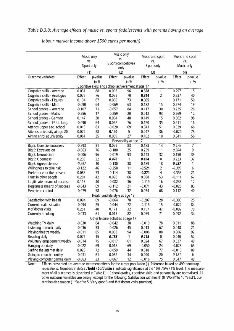
59

Table B.3.8: Average effects of music vs. sports (adolescents with parents having an average

labour market income above 1500 euros per month)

Music only vs.

Sport only

Music only vs.

Sport (competitive) only

Music and sport vs.

Sport only

Music and sport vs.

Music only (1) (2) (3) (4)

Outcome variables Effect p-value in %

Effect p-value in %

Effect p-value in %

Effect p-value in %

Cognitive skills and school achievement at age 17 Cognitive skills - Average 0.031 88 0.006 96 0.328 1 0.297 15 Cognitive skills - Analogies 0.076 76 0.079 70 0.314 2 0.237 40 Cognitive skills - Figures 0.134 67 0.050 73 0.305 1 0.171 50 Cognitive skills - Math -0.090 64 -0.069 63 0.182 15 0.274 19 School grades – Average -0.107 71 -0.057 84 0.117 30 0.225 26 School grades - Maths -0.256 17 -0.259 20 0.012 93 0.269 12 School grades - German 0.147 30 0.094 48 0.149 15 0.002 98 School grades - 1st for. lang. -0.090 64 0.052 76 0.120 35 0.211 16 Attends upper sec. school 0.013 83 -0.020 69 0.041 51 0.029 66 Attends university at age 20 0.072 28 0.140 5 0.047 36 -0.024 75 Aim to enrol at university 0.061 35 0.059 27 0.102 10 0.041 56

Personality at age 17 Big 5: Conscientiousness -0.293 31 0.029 83 0.183 14 0.475 7 Big 5: Extraversion -0.063 76 -0.180 25 0.239 11 0.304 9 Big 5: Neuroticism -0.006 96 -0.019 93 0.143 32 0.150 39 Big 5: Openness 0.233 22 0.478 1 0.454 0 0.223 37 Big 5: Agreeableness -0.297 10 -0.130 38 0.189 18 0.487 1 Willingness to take risk -0.122 46 -0.250 11 -0.521 2 -0.399 6 Preference for the present 0.083 73 -0.114 38 -0.271 4 -0.353 21 Trust in other people 0.201 42 0.096 66 0.088 53 -0.111 67 Legitimate means of success 0.115 40 -0.082 36 -0.119 16 -0.235 12 Illegitimate means of success -0.043 69 -0.112 21 -0.071 43 -0.028 83 Perceived control -0.079 58 -0.076 32 0.034 68 0.112 40

Health and life style at age 18 Satisfaction with health 0.094 69 -0.064 78 -0.207 28 -0.303 25 Current health situation -0.094 25 -0.044 72 -0.115 15 -0.022 84 # of doctor visits 0.251 40 0.171 32 0.157 47 -0.092 79 Currently smoking -0.033 61 0.013 82 0.059 71 0.092 34

Other leisure activities at age 17 Watching TV daily -0.030 64 -0.042 38 -0.019 78 0.011 88 Listening to music daily -0.036 33 -0.026 45 0.013 67 0.048 21 Playing theatre weekly -0.011 85 0.003 94 -0.006 88 0.006 92 Reading daily 0.076 15 0.158 1 0.115 0 0.040 52 Voluntary engagement weekly -0.014 75 -0.017 61 0.024 67 0.037 49 Hanging out daily -0.022 69 0.018 69 -0.050 24 -0.028 65 Surfing the internet daily 0.028 72 -0.059 44 0.018 77 -0.010 89 Going to church monthly -0.031 61 0.052 34 0.090 20 0.121 6 Playing computer games daily -0.063 23 -0.067 12 -0.016 75 0.047 49 Note: Effects presented are average treatment effects for the target population (.). Inference based on 499 bootstrap

replications. Numbers in italics / bold / bold italics indicate significance at the 10% / 5% / 1% level. The measure-ment of all outcomes is described in Table E.1. School grades, cognitive skills and personality are normalised. All other outcome variables are binary, except for the following: Satisfaction with health (0 “Worst” to 10 “Best”), cur-rent health situation (1 “Bad” to 5 “Very good”) and # of doctor visits (number).

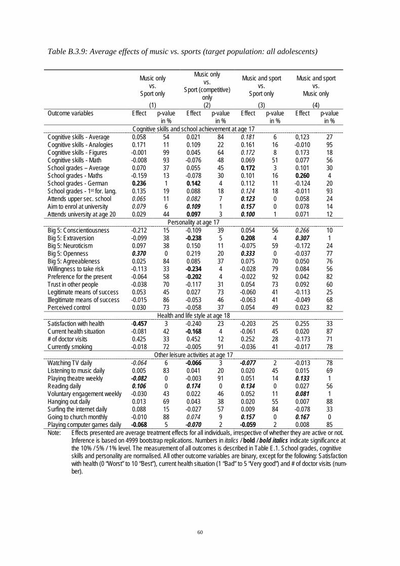
60

Table B.3.9: Average effects of music vs. sports (target population: all adolescents)

Music only vs.

Sport only

Music only vs.

Sport (competitive) only

Music and sport vs.

Sport only

Music and sport vs.

Music only (1) (2) (3) (4)

Outcome variables Effect p-value in %

Effect p-value in %

Effect p-value in %

Effect p-value in %

Cognitive skills and school achievement at age 17 Cognitive skills - Average 0.058 54 0.021 84 0.181 6 0,123 27 Cognitive skills - Analogies 0.171 11 0.109 22 0.161 16 -0.010 95 Cognitive skills - Figures -0.001 99 0.045 64 0.172 8 0.173 18 Cognitive skills - Math -0.008 93 -0.076 48 0.069 51 0.077 56 School grades – Average 0.070 37 0.055 45 0.172 3 0.101 30 School grades - Maths -0.159 13 -0.078 30 0.101 16 0.260 4 School grades - German 0.236 1 0.142 4 0.112 11 -0.124 20 School grades - 1st for. lang. 0.135 19 0.088 18 0.124 18 -0.011 93 Attends upper sec. school 0.065 11 0.082 7 0.123 0 0.058 24 Aim to enrol at university 0.079 6 0.109 1 0.157 0 0.078 14 Attends university at age 20 0.029 44 0.097 3 0.100 1 0.071 12

Personality at age 17 Big 5: Conscientiousness -0.212 15 -0.109 39 0.054 56 0.266 10 Big 5: Extraversion -0.099 38 -0.238 5 0.208 4 0.307 1 Big 5: Neuroticism 0.097 38 0.150 11 -0.075 59 -0.172 24 Big 5: Openness 0.370 0 0.219 20 0.333 0 -0.037 77 Big 5: Agreeableness 0.025 84 0.085 37 0.075 70 0.050 76 Willingness to take risk -0.113 33 -0.234 4 -0.028 79 0.084 56 Preference for the present -0.064 58 -0.202 4 -0.022 92 0.042 82 Trust in other people -0.038 70 -0.117 31 0.054 73 0.092 60 Legitimate means of success 0.053 45 0.027 73 -0.060 41 -0.113 25 Illegitimate means of success -0.015 86 -0.053 46 -0.063 41 -0.049 68 Perceived control 0.030 73 -0.058 37 0.054 49 0.023 82

Health and life style at age 18 Satisfaction with health -0.457 3 -0.240 23 -0.203 25 0.255 33 Current health situation -0.081 42 -0.168 4 -0.061 45 0.020 87 # of doctor visits 0.425 33 0.452 12 0.252 28 -0.173 71 Currently smoking -0.018 72 -0.005 91 -0.036 41 -0.017 78

Other leisure activities at age 17 Watching TV daily -0.064 6 -0.066 3 -0.077 2 -0.013 78 Listening to music daily 0.005 83 0.041 20 0.020 45 0.015 69 Playing theatre weekly -0.082 0 -0.003 91 0.051 14 0.133 1 Reading daily 0.106 0 0.174 0 0.134 0 0.027 56 Voluntary engagement weekly -0.030 43 0.022 46 0.052 11 0.081 1 Hanging out daily 0.013 69 0.043 38 0.020 55 0.007 88 Surfing the internet daily 0.088 15 -0.027 57 0.009 84 -0.078 33 Going to church monthly -0.010 88 0.074 9 0.157 0 0.167 0 Playing computer games daily -0.068 5 -0.070 2 -0.059 2 0.008 85 Note: Effects presented are average treatment effects for all individuals, irrespective of whether they are active or not.

Inference is based on 4999 bootstrap replications. Numbers in italics / bold / bold italics indicate significance at the 10% / 5% / 1% level. The measurement of all outcomes is described in Table E.1. School grades, cognitive skills and personality are normalised. All other outcome variables are binary, except for the following: Satisfaction with health (0 “Worst” to 10 “Best”), current health situation (1 “Bad” to 5 “Very good”) and # of doctor visits (num-ber).

61

B.4 Robustness analysis

Table B.4.1: Average effects of music vs. sports (additional requirement for being considered

to play music: take music lessons outside of school)

Music only vs.

Sport only

Music only vs.

Sport (competitive) only

Music and sport vs.

Sport only

Music and sport vs.

Music only (1) (2) (3) (4)

Outcome variables Effect p-value in %

Effect p-value in %

Effect p-value in %

Effect p-value in %

Cognitive skills and school achievement at age 17 Cognitive skills - Average 0.122 32 0.156 22 0.262 2 0.162 26 Cognitive skills - Analogies 0.186 15 0.226 2 0.256 2 0.089 55 Cognitive skills - Figures 0.159 18 0.189 9 0.339 0 0.198 17 Cognitive skills - Math -0.009 94 0.001 98 0.073 52 0.100 47 School grades – Average 0.063 47 0.116 11 0.239 0 0.192 6 School grades - Maths -0.113 23 -0.008 91 0.254 0 0.371 0 School grades - German 0.229 0 0.195 1 0.123 7 -0.086 39 School grades - 1st for. lang. 0.060 49 0.100 15 0.140 9 0.094 41 Attends upper sec. school 0.140 0 0.097 1 0.173 0 0.052 29 Attends university at age 20 0.073 10 0.075 8 0.122 0 0.056 29 Aim to enrol at university 0.169 0 0.139 0 0.227 0 0.071 16

Personality at age 17 Big 5: Conscientiousness -0.079 48 0.044 59 0.105 24 0.176 17 Big 5: Extraversion -0.245 2 -0.223 4 0.057 53 0.300 2 Big 5: Neuroticism 0.081 51 0.267 2 0.081 32 0.001 98 Big 5: Openness 0.392 0 0.401 0 0.392 0 -0.001 97 Big 5: Agreeableness 0.119 28 0.125 14 0.264 0 0.142 33 Willingness to take risk -0.181 11 -0.303 0 -0.109 25 0.063 68 Preference for the present -0.098 37 -0.237 1 -0.164 10 -0.067 65 Trust in other people 0.250 5 0.005 95 0.256 1 0.009 94 Legitimate means of success 0.028 73 -0.040 56 -0.030 67 -0.054 56 Illegitimate means of success 0.017 86 0.037 78 -0.083 27 -0.094 54 Perceived control 0.173 6 0.000 98 0.094 19 -0.062 71

Health and life style at age 18 Satisfaction with health -0.243 14 -0.211 15 -0.091 61 0.132 59 Current health situation -0.131 10 -0.119 8 0.032 61 0.161 8 # of doctor visits 0.103 69 0.297 35 -0.127 53 -0.192 46 Currently smoking -0.071 12 -0.038 31 -0.102 0 -0.041 45

Other leisure activities at age 17 Watching TV daily -0.096 2 -0.111 1 -0.139 0 -0.045 37 Listening to music daily -0.001 96 0.016 49 0.010 80 0.011 77 Playing theatre weekly -0.036 27 0.001 95 0.053 9 0.090 2 Reading daily 0.102 2 0.126 0 0.120 0 0.024 65 Voluntary engagement weekly -0.025 46 -0.009 82 0.090 1 0.119 1 Hanging out daily -0.015 70 0.048 25 0.008 81 0.027 55 Surfing the internet daily 0.031 61 -0.009 87 0.030 57 0.004 97 Going to church monthly 0.024 60 0.049 25 0.230 0 0.201 0 Playing computer games daily -0.120 0 -0.101 0 -0.074 3 0.040 59 Note: Effects presented are average treatment effects for the target population (.). Inference based on 999 bootstrap

replications. Numbers in italics / bold / bold italics indicate significance at the 10% / 5% / 1% level. The measure-ment of all outcomes is described in Table E.1. School grades, cognitive skills and personality are normalised. All other outcome variables are binary, except for the following: Satisfaction with health (0 “Worst” to 10 “Best”), cur-rent health situation (1 “Bad” to 5 “Very good”) and # of doctor visits (number).

62

Table B.4.2: Average effects of music vs. sports (in addition to standard definition, adoles-

cents are considered as active if they play music or sports at least monthly)

Music only vs.

Sport only

Music only vs.

Sport (competitive) only

Music and sport vs.

Sport only

Music and sport vs.

Music only (1) (2) (3) (4)

Outcome variables Effect p-value in %

Effect p-value in %

Effect p-value in %

Effect p-value in %

Cognitive skills and school achievement at age 17 Cognitive skills - Average 0.082 41 -0.050 60 0.209 2 0.128 26 Cognitive skills - Analogies 0.182 15 0.098 26 0.255 0 0.076 56 Cognitive skills - Figures -0.003 97 0.013 90 0.326 0 0.329 1 Cognitive skills - Math 0.030 76 -0.171 6 -0.042 70 -0.073 60 School grades – Average 0.038 57 0.159 6 0.172 1 0.137 10 School grades - Maths -0.110 14 -0.014 84 0.141 5 0.248 1 School grades - German 0.154 2 0.218 0 0.127 3 -0.021 79 School grades - 1st for. lang. 0.079 31 0.180 3 0.119 4 0.046 60 Attends upper sec. school 0.100 1 0.055 12 0.146 0 0.049 27 Attends university at age 20 0.056 16 0.077 2 0.073 5 0.020 71 Aim to enrol at university 0.115 0 0.105 0 0.171 0 0.059 18

Personality at age 17 Big 5: Conscientiousness -0.169 18 -0.003 98 0.091 47 0.259 4 Big 5: Extraversion -0.223 4 -0.239 1 0.194 4 0.417 0 Big 5: Neuroticism 0.087 40 0.056 58 -0.098 31 -0.186 18 Big 5: Openness 0.495 0 0.357 0 0.443 0 -0.052 66 Big 5: Agreeableness -0.044 69 0.096 29 0.144 15 0.188 12 Willingness to take risk -0.100 35 -0.243 4 0.019 87 0.117 41 Preference for the present -0.057 64 -0.168 19 -0.162 10 -0.106 39 Trust in other people -0.195 10 -0.077 42 0.169 10 0.364 1 Legitimate means of success -0.059 50 -0.010 89 -0.047 55 0.012 92 Illegitimate means of success -0.093 21 -0.026 71 -0.003 97 0.089 44 Perceived control 0.065 44 0.017 84 0.082 26 0.017 85

Health and life style at age 18 Satisfaction with health -0.002 98 -0.238 9 -0.002 97 0.001 98 Current health situation -0.065 58 -0.150 2 -0.015 82 0.049 65 # of doctor visits 0.403 16 0.712 40 0.387 46 -0.022 96 Currently smoking -0.115 0 -0.057 10 -0.066 16 0.047 52

Other leisure activities at age 17 Watching TV daily -0.081 3 -0.094 0 -0.074 5 0.006 90 Listening to music daily -0.004 89 -0.003 87 0.033 4 0.037 11 Playing theatre weekly 0.086 9 0.057 4 0.091 1 0.006 92 Reading daily 0.105 2 0.155 0 0.131 0 0.025 58 Voluntary engagement weekly 0.050 14 0.069 2 0.147 0 0.097 4 Hanging out daily 0.006 84 0.109 1 0.023 53 0.017 73 Surfing the internet daily -0.091 10 -0.164 0 -0.065 13 0.028 66 Going to church monthly 0.068 15 0.063 14 0.208 0 0.140 2 Playing computer games daily -0.057 12 -0.096 0 -0.049 13 0.007 87 Note: Effects presented are average treatment effects for the target population (.). Inference based on 999 bootstrap

replications. Numbers in italics / bold / bold italics indicate significance at the 10% / 5% / 1% level. The measure-ment of all outcomes is described in Table E.1. School grades, cognitive skills and personality are normalised. All other outcome variables are binary, except for the following: Satisfaction with health (0 “Worst” to 10 “Best”), cur-rent health situation (1 “Bad” to 5 “Very good”) and # of doctor visits (number).

63

Table B.4.3: Average effects of music vs. sports (using a different common support rule)

Music only vs.

Sport only

Music only vs.

Sport (competitive) only

Music and sport vs.

Sport only

Music and sport vs.

Music only (1) (2) (3) (4)

Outcome variables Effect p-value in %

Effect p-value in %

Effect p-value in %

Effect p-value in %

Cognitive skills and school achievement at age 17 Cognitive skills - Average 0.100 28 0.103 27 0.302 0 0.213 6 Cognitive skills - Analogies 0.080 58 0.198 5 0.269 0 0.201 10 Cognitive skills - Figures 0.161 10 0.167 5 0.345 0 0.191 10 Cognitive skills - Math 0.029 74 -0.065 48 0.126 15 0.107 32 School grades – Average 0.058 44 0.124 8 0.193 0 0.152 8 School grades - Maths -0.086 26 -0.025 72 0.175 2 0.264 1 School grades - German 0.171 2 0.204 0 0.137 4 -0.012 89 School grades - 1st for. lang. 0.068 36 0.132 6 0.106 26 0.055 52 Attends upper sec. school 0.081 6 0.097 1 0.190 0 0.123 3 Attends university at age 20 0.056 15 0.073 3 0.128 0 0.078 9 Aim to enrol at university 0.126 0 0.118 0 0.218 0 0.103 4

Personality at age 17 Big 5: Conscientiousness -0.054 53 -0.047 63 0.106 23 0.168 9 Big 5: Extraversion -0.121 27 -0.173 7 0.114 17 0.250 5 Big 5: Neuroticism 0.014 92 0.139 14 0.032 70 0.003 97 Big 5: Openness 0.411 0 0.377 0 0.413 0 -0.003 96 Big 5: Agreeableness 0.022 82 0.080 38 0.327 0 0.319 2 Willingness to take risk -0.114 28 -0.236 1 -0.151 25 -0.026 84 Preference for the present -0.154 12 -0.139 14 -0.185 3 -0.035 79 Trust in other people 0.028 84 0.001 99 0.249 1 0.228 5 Legitimate means of success 0.044 57 0.045 48 -0.007 93 -0.063 48 Illegitimate means of success 0.038 80 -0.047 49 -0.098 31 -0.132 52 Perceived control 0.108 25 -0.081 22 0.042 49 -0.056 62

Health and life style at age 18 Satisfaction with health -0.134 37 -0.421 0 -0.015 89 0.128 43 Current health situation -0.119 9 -0.175 0 -0.039 51 0.084 26 # of doctor visits 0.352 52 0.942 2 0.031 90 -0.320 60 Currently smoking -0.040 43 -0.022 53 -0.104 0 -0.075 25

Other leisure activities at age 17 Watching TV daily -0.097 2 -0.096 0 -0.122 0 -0.028 49 Listening to music daily 0.018 47 0.026 20 0.009 80 -0.009 87 Playing theatre weekly -0.029 34 0.011 71 0.010 85 0.043 32 Reading daily 0.082 3 0.147 0 0.126 0 0.051 21 Voluntary engagement weekly 0.019 52 0.020 50 0.109 0 0.091 3 Hanging out daily 0.020 57 0.062 6 0.008 82 -0.009 83 Surfing the internet daily 0.041 41 -0.023 63 0.027 55 -0.020 72 Going to church monthly 0.053 20 0.073 8 0.197 0 0.148 0 Playing computer games daily -0.072 1 -0.088 0 -0.064 2 0.006 88 Note: Effects presented are average treatment effects for the target population (.).The common support quantile is now

fixed to 97%. Inference based on 999 bootstrap replications (except column 2, in which p-values do not take into account that the propensity score is estimated). Numbers in italics / bold / bold italics indicate significance at the 10% / 5% / 1% level. The measurement of all outcomes is described in Table E.1. School grades, cognitive skills and personality are normalised. All other outcome variables are binary, except for the following: Satisfaction with health (0 “Worst” to 10 “Best”), current health situation (1 “Bad” to 5 “Very good”) and # of doctor visits (number).

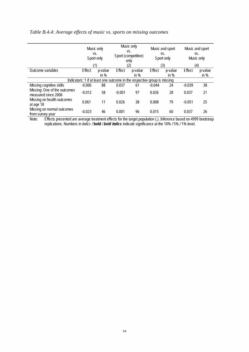
64

Table B.4.4: Average effects of music vs. sports on missing outcomes

Music only vs.

Sport only

Music only vs.

Sport (competitive) only

Music and sport vs.

Sport only

Music and sport vs.

Music only (1) (2) (3) (4)

Outcome variables Effect p-value in %

Effect p-value in %

Effect p-value in %

Effect p-value in %

Indicators: 1 if at least one outcome in the respective group is missing Missing cognitive skills -0.006 88 0.037 61 -0.044 24 -0.039 38 Missing: One of the outcomes measured since 2006 -0.012 58 -0.001 97 0.026 28 0.037 21 Missing on health outcomes at age 18 0.061 11 0.026 38 0.008 79 -0.051 25 Missing on normal outcomes from survey year -0.023 46 0.001 96 0.015 60 0.037 26

Note: Effects presented are average treatment effects for the target population (.). Inference based on 4999 bootstrap replications. Numbers in italics / bold / bold italics indicate significance at the 10% / 5% / 1% level.

65

Table B.4.5: Average effects of music vs. sports (using survey weights)

Music only vs.

Sport only

Music only vs.

Sport (competitive) only

Music and sport vs.

Sport only

Music and sport vs.

Music only (1) (2) (3) (4)

Outcome variables Effect p-value in %

Effect p-value in %

Effect p-value in %

Effect p-value in %

Cognitive skills and school achievement at age 17 Cognitive skills - Average 0.169 16 0.008 93 0.267 0 0.100 45 Cognitive skills - Analogies 0.246 4 0.093 36 0.292 0 0.047 74 Cognitive skills - Figures 0.184 16 0.051 62 0.184 4 0.002 99 Cognitive skills - Math 0.020 85 -0.114 27 0.107 26 0.088 50 School grades – Average -0.006 95 0.070 39 0.122 10 0.135 18 School grades - Maths -0.175 19 -0.036 60 0.090 22 0.263 1 School grades - German 0.168 3 0.115 16 0.084 20 -0.072 44 School grades - 1st for. lang. 0.039 63 0.096 19 0.095 21 0.063 52 Attends upper sec. school 0.131 0 0.065 9 0.156 0 0.032 53 Attends university at age 20 0.023 73 0.084 1 0.111 0 0.088 7 Aim to enrol at university 0.097 4 0.093 0 0.182 0 0.090 7

Personality at age 17 Big 5: Conscientiousness -0.161 15 -0.027 77 0.107 19 0.263 3 Big 5: Extraversion -0.219 4 -0.181 3 0.174 1 0.390 0 Big 5: Neuroticism 0.172 9 0.173 5 -0.002 96 -0.175 12 Big 5: Openness 0.355 0 0.379 0 0.377 0 0.023 86 Big 5: Agreeableness 0.099 43 0.094 30 0.234 1 0.135 32 Willingness to take risk -0.070 54 -0.227 3 -0.019 83 0.053 70 Preference for the present -0.048 61 -0.263 0 -0.208 1 -0.152 17 Trust in other people -0.083 41 -0.013 92 0.197 2 0.283 3 Legitimate means of success 0.043 54 -0.041 55 -0.131 9 -0.174 6 Illegitimate means of success -0.014 89 -0.129 9 -0.032 62 -0.020 82 Perceived control 0.035 69 0.020 80 0.073 19 0.035 72

Health and life style at age 20 Satisfaction with health -0.357 19 -0.140 28 0.125 48 0.481 1 Current health situation -0.188 4 -0.093 12 0.024 76 0.214 2 # of doctor visits 0.709 58 0.238 46 -0.051 86 -0.750 22 Currently smoking -0.046 32 -0.050 14 -0.128 0 -0.083 9

Other leisure activities at age 17 Watching TV daily -0.060 8 -0.080 1 -0.093 0 -0.034 43 Listening to music daily 0.017 51 0.035 10 0.021 39 0.005 87 Playing theatre weekly -0.054 6 -0.022 50 0.051 8 0.104 1 Reading daily 0.091 1 0.137 0 0.144 0 0.057 22 Voluntary engagement weekly -0.020 57 -0.006 87 0.070 1 0.094 1 Hanging out daily 0.002 94 0.072 1 0.018 55 0.017 69 Surfing the internet daily 0.045 43 -0.016 75 0.019 64 -0.027 68 Going to church monthly 0.013 76 0.052 26 0.197 0 0.184 0 Playing computer games daily -0.074 4 -0.066 1 -0.053 7 0.020 64 Note: Effects presented are average treatment effects for the target population (.). Inference based on 499 bootstrap

replications (except columns 1 and 4, in which p-values do not take into account that the propensity score is esti-mated). Numbers in italics / bold / bold italics indicate significance at the 10% / 5% / 1% level. The measurement of all outcomes is described in Table E.1. School grades, cognitive skills and personality are normalised. All other outcome variables are binary, except for the following: Satisfaction with health (0 “Worst” to 10 “Best”), current health situation (1 “Bad” to 5 “Very good”) and # of doctor visits (number).

66

Appendix C: Details on the matching estimator

Table C.1 gives the detailed matching protocol used. See Huber, Lechner, and Wunsch

(2013) and Huber, Lechner, and Steinmayr (2012) for further details on the implementation

and the properties of this estimator, including trimming and common support rules.

Table C.1: Matching protocol for the estimation of a counterfactual outcome and the effects

Step A-1 Choose one observation in the subsample defined by d=1 and delete it from that pool. Step B-1 Find an observation in the subsample defined by d=0 that is as close as possible to the one chosen in step A-

1) in terms of (𝑥), 𝑥�. 'Closeness' is based on the Mahalanobis distance. Step C-1 Repeat A-1) and B-1) until no observation with d=1 is left. Step D-1 Compute the maximum distance (dist) obtained for any comparison between a member of the reference

distribution and matched comparison observations. Step A-2 Repeat A-1). Step B-2 Repeat B-1). If possible, find other observations in the subsample of d=0 that are at least as close as R * dist

to the one chosen in step A-2). Do not remove these observations, so that they can be used again. Compute weights for all chosen comparisons observations that are proportional to their distance. Normalise the weights such that they add to one.

Step C-2 Repeat A-2) and B-2) until no participant in d=1 is left. Step D-2 D-2) For any potential comparison observation, add the weights obtained in A-2) and B-2). Step E Using the weights 𝑤(𝑥𝑖) obtained in D-2), run a weighted linear regression of the outcome variable on the

variables used to define the distance (and an intercept). Step F-1 Predict the potential outcome 𝑦0(𝑥𝑖) of every observation using the coefficients of this regression: 𝑦�0(𝑥𝑖) . Step F-2 Estimate the bias of the matching estimator for 𝐸(𝑌0|𝐷 = 1) as: ∑ (1−𝑑𝑖)𝑤𝑖𝑦�0(𝑥𝑖)

𝑁0− 𝑑𝑖𝑦�0(𝑥𝑖)

𝑁1𝑁𝑖=1 .

Step G Using the weights obtained by weighted matching in D-2), compute a weighted mean of the outcome vari-ables in d=0. Subtract the bias from this estimate to get 𝐸(𝑌0|𝐷 = 1).

Note: R is set to 150%. Gender is used as additional matching variable ( x ). The weight of the propensity score coming from the Mahalanobis metric is multiplied by 5. Control observations with weights larger than 5% are removed.

Table C.1 shows how to compute the average treatment effects on the treated (ATET).

The average treatment effects on the non-treated (ATENT) are computed in the same way but

the role of treated and controls are reversed in the algorithm. The average treatment effect

(ATE) is computed by aggregating both effects using the treatment share (ATE = ATET x

P(D=1) + ATENT x P(D=0)). These estimations are performed for each of the six subsamples

separately. The weights used to aggregate these estimates over specific groups or the popula-

tion are proportional to the number of treated (for the ATET) / controls (ATENT) / popula-

tions (ATE) in the respective subsamples.

See also Huber, Lechner, and Steinmayr (2012) for operational details of this estimator.

The particular version of this estimator used is the RAD_MATCH Gauss package version

67

3.2.1. It has the feature that sampling weights may be accounted for in general. Furthermore,

bootstrap inference as described in Huber, Lechner and Steinmayr (2012) is based on weights

that are combination of sampling weights, matching weights as well as regression weights.

The improved bootstrap smoother as proposed by Racine and MacKinnon (2007) is used to

economize on the required bootstrap replications. In addition, the variable gender is used as

additional variables in the Mahalanobis step, in which the propensity score is overweighed by

a factor of 5. The distance measure is set to 150%.

68

Appendix D: Robustness with respect to the validity of the

selection-on-observables assumption

D.1 Instrumental variable estimation

Concepts and instruments used

We need an instrumental variable (IV) as an exogenous source of variation in the choice

of an extracurricular activity. This IV should induce the individual to choose music rather

than sports: we use an indicator of whether either parent played a musical instrument in their

youth.21 It is a binary indicator coded to “1” if either parent declares having played a musical

instrument, “0” otherwise.22 In order to identify a causal effect, this IV must be strong and

valid.

We argue that parental engagement in musical activities during their own adolescence

is a strong IV for the child’s decision to play music rather than or in addition to sports. The

relevance of that variable can be justified both theoretically and empirically. Parents play an

important role in choosing their children’s extracurricular activities, given that they provide

financial, logistic and psychological support (Gustafson and Rhodes 2006). Following a clas-

sical Becker-type reasoning (Becker 1965), the decision to enrol in music classes or a sports

club is likely to be motivated by maximizing utility, both with respect to current pleasure and

future investments in skills.23 Assuming that individuals have imperfect information, personal

21 While no age is specified for this question in the questionnaire, it is preceded by other questions concerning the period

when the individual was 15 years old.

22 This question relative to adolescent leisure activities has been asked in the SOEP Biography Questionnaire since 2001, a questionnaire that is completed by all survey participants in the year they enter the SOEP. Therefore, the instrument is only available for parents who entered the SOEP in 2001 or later. This is problematic, since it dramatically reduces our sample size. New households enter the SOEP due to the decision to increase the overall sample size of the study. The year of entry into the panel study is therefore unrelated and exogenous to our question of interest. Approximately half of our sample entered the SOEP in 2001 or later and answered the relevant question in the SOEP Biography Questionnaire.

23 In such models of family decisions, the utility of the parent and the utility of the child are often considered to be the same.

69

experience is likely to influence their choice with respect to their child’s leisure activity. In

addition, the choice of activity is likely to depend on taste. This reinforces the relevance of

our IV. Taste is shaped either by education or repeated consumption (Garboua and Montmar-

quette 1996, Lunn and Kelly 2009, Seaman 2006). Hence, the child is likely to share the same

taste as her parents. Hille and Schupp (2015) argue that the parents’ taste for the arts is a very

strong predictor of their child’s enrolment into music practice.

The crucial assumption for an IV to be valid is that it has no direct effect on the out-

come. This assumption is known as exogeneity or mean exclusion restriction (Frölich 2007).

The mean exclusion restriction may be invalid due to reverse causality, observable and unob-

servable characteristics determining the IV as well as a direct effect of the IV through a chan-

nel other than the treatment. We discuss each of these potential violations in the following.

Reverse causality can be ruled out since the IV is measured prior to the child’s birth.

Still, the IV – childhood musical activity of the parents – may affect the outcome due to the

influence of its determinants. If education or other parental characteristics – besides providing

an incentive to engage with music – influence the child’s skill development, the exogeneity

assumption is violated. Parental participation in artistic activities is linked to their level of

education and their socio-economic environment. These characteristics are correlated with

their labour-market success and thus with their child’s development. We take this endogeneity

into account by adding covariates (the same we use for in the selection-on-observables

framework in the main part of this paper).24

A final source of violation of the exogeneity assumption exists, if the IV has a direct ef-

fect on the outcomes due to the effects of parental activities on parental skills. If being active

in music has affected parental skill development differently than being active in sports and if

24 We need to control for these characteristics only if they are different between sports and music or if their influence on

child outcomes differ. Conversely, if the determinants of parental sports and music activities as well as their effect on child outcomes are the same, we can ignore them in our estimation. In this case, they would characterize both treated and non-treated in the same way and thereby mechanically offset each other’s effect.

70

this has consequences on the child’s skill development, our IV is no longer exogenous. Music

activities might have benefited the parents’ skills during childhood and youth. While person-

ality has been found malleable during childhood (e.g. Cobb-Clark and Schurer 2012, Donne-

lan and Lucas 2008, Heckman and Kautz 2012, Specht, Egloff and Schmukle 2011), it is con-

sidered stable among adults (Pervin, Cervone and John 2005). We control for parental person-

ality, which may have been affected by childhood leisure activities. Some of the advantages

resulting from parental differences in past leisure activity are taken into account by control-

ling for education, income and labour market situation as described above.

Finally, the identification of the local average treatment effect using IV requires the as-

sumption of monotonicity (Frölich 2007). We need to assume that no adolescent chooses to

become active in sports rather than music, even though their parents were engaged in artistic

activities several years before. While we cannot rule out the existence of rebellious children,

we argue that, given the age at which children decide between music and sports, they are un-

likely to drive our results and that the monotonicity assumption is satisfied due to our sample

choice.25

Sample selection and descriptive statistics

The subsample for which the IV is available is roughly half the size of the original sam-

ple and somewhat different. The high-income group is overrepresented and immigrants as

well as East Germans are underrepresented. Being part of the SOEP design, these differences

in sample composition are exogenous to our questions of interest. We expect mean outcomes

to differ from the original sample.

25 Active adolescents are mostly less rebellious than their inactive peers. Given that our sample is restricted to individuals

who engage in at least one activity or sample contains those who are more likely to follow the choices of their parents.

71

Results

As suggested by Frölich (2007), we estimate the LATE non-parametrically by using a

propensity score to reduce dimensionality. This is necessary, given that the sample is rela-

tively small and that we need to control for a large number of covariates. The estimation of

the LATE with covariates (propensity score in our case) is equivalent to the computation of

two matching estimators: the effect of the instrument on the outcome divided by the effect of

the instrument on the treatment (conditional on a set of covariates). This effect concerns

solely the subpopulation of compliers: individuals who react to the instrument (i.e. adoles-

cents who play music because at least one of their parents was artistically active at the age of

16).

The results of the estimations are reported in table D.1. The first stage represents the ef-

fect of the instrument on the probability of being treated. The fact that at least one of the par-

ents played a musical instrument during their adolescence is a good predictor of the probabil-

ity that the adolescent herself is engaged in music. As stated above, the LATE is different

from the ATE; therefore, the results cannot be directly compared to the main results of the

paper.26 We find that practicing music instead of sports has a detrimental effect on school

grades in mathematics for the complier population (columns 1 and 2 of Table D.1.). Last,

practicing music instead of doing sport competitively increases the openness of the adoles-

cent.

26 Moreover, the samples on which the estimations are run are different.

72

Table D.1: Average effects of music vs. sports (IV estimations)

Music only vs.

Sport only

Music only vs.

Sport (competitive) only

Music and sport vs.

Sport only (1) (2) (3)

Outcome variables Effect p-value in %

Effect p-value in %

Effect p-value in %

First stage 0.071 1 0.144 0 0.099 0 Cognitive skills and school achievement

Cognitive skills - Average 0.593 89 0.293 88 0.424 94 Cognitive skills - Analogies -2.460 65 -1.214 60 -1.760 66 Cognitive skills - Figures -0.962 84 -0.475 81 -0.688 85 Cognitive skills - Math 4.456 54 2.199 48 3.188 81 School grades – Average -0.907 17 -0.448 13 -0.649 23 School grades - Maths -2.614 6 -1.290 2 -1.870 18 School grades - German -0.326 68 -0.161 63 -0.234 67 School grades - 1st for. lang. -0.226 79 -0.112 76 -0.162 88 Attends upper sec. school 0.126 75 0.062 69 0.090 81 Attends university at age 20 -0.561 18 -0.277 11 -0.402 22 Aim to enrol at university -0.057 86 -0.028 85 -0.041 88

Personality Big 5: Conscientiousness -0.130 56 -0.064 50 -0.093 75 Big 5: Extraversion -0.014 94 -0.007 94 -0.010 96 Big 5: Neuroticism 0.150 48 0.074 40 0.107 66 Big 5: Openness 0.297 26 0.147 9 0.213 27 Big 5: Agreeableness 0.213 27 0.105 18 0.152 67 Willingness to take risk 0.944 69 0.466 66 0.676 71 Preference for the present -0.315 26 -0.156 16 -0.226 39 Trust in other people -0.143 46 -0.071 42 -0.102 56 Legitimate means of success -0.054 61 -0.027 54 -0.039 63 Illegitimate means of success 0.103 44 0.051 39 0.074 64 Perceived control 0.082 55 0.041 45 0.059 69

Health and life style at age 20 Satisfaction with health -0.429 86 -0.212 83 -0.307 87 Current health situation -0.313 75 -0.155 72 -0.224 83 # of doctor visits 2.641 43 1.304 35 1.889 50 Currently smoking -0.334 55 -0.165 49 -0.239 61

Other leisure activities at age 17 Watching TV daily -0.092 82 -0.045 79 -0.066 84 Listening to music daily 0.147 56 0.072 52 0.105 68 Playing theatre weekly 0.047 89 0.023 88 0.034 92 Reading daily 0.371 48 0.183 37 0.266 42 Voluntary engagement weekly 0.475 17 0.235 13 0.340 49 Hanging out daily -0.023 95 -0.011 95 -0.017 96 Surfing the internet daily 0.722 43 0.356 30 0.516 77 Going to church monthly 0.572 35 0.282 23 0.409 57 Playing computer games daily 0.412 43 0.203 30 0.294 75 Note: Inference based on 399 bootstrap replications. Numbers in italics / bold / bold italics indicate significance at the

10%/5%/1% level. Contrary to the estimations in other tables of this paper, school grades, cognitive skills and per-sonality are not normalised, but measured from 0 to 20 for cognitive skill, from 6 to 1 for school grades and from 0 to 1 for personality. The measurement of all other outcomes is described in Table E.1. Expectations are measured in percentage points. All other outcome variables are binary, except for some health measures as indicated.

73

D.2 Sensitivity test – Ichino, Mealli and Nannicini (2008)

The test relies on the simulation of a confounder, U, that is correlated to the outcomes

and to the treatment. The sensitivity of the specification to a violation of the CIA is assessed

by comparing results with the simulated confounder U and results without. The confounder U

is binary and independent of included covariates.27 The confounder is simulated such that its

probability (pij) for taking a value of 1 varies for the four strata defined by the outcome and

the treatment i.e. pij=P(U=1/D=i, Y=j), i,j∈{0,1} (Y denotes the outcome variable and D de-

notes the treatment). Setting pij to 0.5 for all cases would therefore be the same as simulating a

confounder U that does not bias the results. This probability scenario is similar to the “without

the confounder U” scenario (scenario 1). It is used as the baseline when comparing results. To

simulate a confounder U which pij varies with treatment and outcome, we use the correlation

pattern of an important observed confounder: gender (scenario 2). In other words, the proba-

bility (pij) is similar to the probability for gender, which varies among the strata (and among

the different treatments that we use). By doing so we test the sensitivity of our specification to

a missing unobserved confounder that is correlated to treatment and potential outcome in the

same way as gender is. We choose gender because it is the most important confounder in

terms of size and significance in the p-score. Furthermore, we believe that the unobserved

confounders are closely related to gender (behaviours, parents’ education and preferences, for

example). A third scenario is simulated in which we use the correlation pattern of another

important covariate: the recommendation for upper secondary school (scenario 3). This co-

variate is also an important confounder which is used as a proxy for cognitive skills. We be-

lieve that the unobserved confounders might be correlated with this proxy.

Following Ichino, Mealli and Nannicini (2008) suggestion, we repeat the simulations

several times and take the mean of the effects over the simulations. We draw 19 times U (i.e. 27 We choose this specific framework for simplification. However, the results should hold with a continuous confounder and

without covariates.

74

we have 19 random realisations of U for each observation) within each bootstrap replication

and use 99 bootstrap replications for each scenario. Then, we compare the results between the

baseline (pij = 0.5, ∀ i,j) and the two biased scenario (scenario 2 and 3). The deviations from

the baseline results and their significance are reported in Table D.2.1 for scenario 2 and in

Table D.2.2 for scenario 3. The deviation is computed for the ATE for the target population

with linear bias correction for the 4 treatments. The deviation is never significant at the 5%

threshold. Our specification is not sensitive to a violation of the CIA in the tested scenario.

75

Table D.2.1: Average effects of music vs. sports (scenario 2: a confounder similar to gender)

Music only vs.

Sport only

Music only vs.

Sport (competitive) only

Music and sport vs.

Sport only

Music and sport vs.

Music only (1) (2) (3) (4)

Outcome variables Difference to baseline

Difference to baseline

Difference to baseline

Difference to baseline

Cognitive skills and school achievement at age 17 Cognitive skills - Average 0.007 -0.020 0.001 -0.015 Cognitive skills - Analogies -0.028 -0.025 0.031 -0.003 Cognitive skills - Figures 0.005 0.011 -0.008 -0.017 Cognitive skills - Math 0.033 -0.027 -0.012 -0.006 School grades – Average -0.004 0.024 0.008 -0.016 School grades - Maths -0.012 0.002 0.014 -0.016 School grades - German -0.001 0.038 0.005 -0.019 School grades - 1st for. lang. 0.008 0.009 0.001 -0.005 Attends upper sec. school -0.008 -0.011 0.003 0.014 Attends university at age 20 0.003 -0.007 -0.006 0.028 Aim to enrol at university 0.001 -0.002 0.005 0.012

Personality at age 17 Big 5: Conscientiousness 0.013 0.004 -0.034 0.012 Big 5: Extraversion 0.040 0.018 -0.041 0.085 Big 5: Neuroticism 0.007 -0.007 0.031 0.007 Big 5: Openness -0.024 0.008 -0.012 0.081 Big 5: Agreeableness 0.015 -0.013 -0.006 -0.008 Willingness to take risk 0.035 0.002 -0.006 0.028 Preference for the present -0.030 -0.002 0.008 0.032 Trust in other people 0.006 0.058 0.006 -0.029 Legitimate means of success -0.006 0.009 0.022 -0.034 Illegitimate means of success -0.016 0.033 0.008 0.008 Perceived control -0.008 0.030 -0.023 0.039

Health and life style at age 20 Satisfaction with health -0.008 -0.050 0.026 0.052 Current health situation 0.017 0.015 -0.003 -0.032 # of doctor visits 0.036 0.228 0.072 0.119 Currently smoking -0.010 0.001 0.003 0.007

Other leisure activities at age 17 Watching TV daily 0.001 -0.005 0.001 0.010 Listening to music daily 0.005 -0.004 -0.001 -0.003 Playing theatre weekly 0.002 0.007 0.001 -0.006 Reading daily -0.002 -0.009 -0.008 0.015 Voluntary engagement weekly -0.010 -0.001 -0.005 -0.005 Hanging out daily 0.000 -0.006 0.010 0.003 Surfing the internet daily -0.015 -0.010 0.022 0.011 Going to church monthly 0.002 -0.019 -0.001 -0.012 Playing computer games daily 0.004 -0.010 -0.004 0.001 Note: Difference of effects in confounding scenario to baseline scenario. For the confounding scenario, a confounder U is

simulated with probabilities: P(U=1|Y=1,D=1); P(U=1|Y=0,D=1); P(U=1|Y=1,D=0); P(U=1|Y=0,D=0) according to those of the variable gender. Inference based on 99 bootstrap replications and 19 draws of simulated binary con-founder; quantile method, smoothed version, linear bias adjustment, symmetric p-values used. None of the differ-ences are statistically significant at the 10% level. The measurement of all outcomes is described in Table E.1. School grades, cognitive skills and personality are normalised. All other outcome variables are binary, except for the following: Satisfaction with health (0 “Worst” to 10 “Best”), current health situation (1 “Bad” to 5 “Very good”) and # of doctor visits (number).

76

Table D.2.2: Average effects of music vs. sports (scenario 3: a confounder similar to the rec-

ommendation for upper secondary school)

Music only vs.

Sport only

Music only vs.

Sport (competitive) only

Music and sport vs.

Sport only

Music and sport vs.

Music only (1) (2) (3) (4)

Outcome variables Difference to baseline

Difference to baseline

Difference to baseline

Difference to baseline

Cognitive skills and school achievement at age 17 Cognitive skills - Average -0.027 0.004 -0.011 0.010 Cognitive skills - Analogies -0.033 0.002 0.001 0.005 Cognitive skills - Figures -0.009 0.015 -0.017 -0.033 Cognitive skills - Math -0.020 -0.007 -0.014 0.026 School grades – Average 0.002 -0.014 0.008 -0.002 School grades - Maths 0.003 -0.012 0.007 -0.006 School grades - German 0.004 -0.008 0.001 0.001 School grades - 1st for. lang. -0.005 -0.014 0.012 0.007 Attends upper sec. school -0.011 -0.007 -0.003 0.007 Attends university at age 20 -0.018 -0.001 -0.015 0.016 Aim to enrol at university -0.008 -0.001 0.000 0.001

Personality at age 17 Big 5: Conscientiousness -0.026 0.027 -0.014 0.000 Big 5: Extraversion 0.009 -0.026 -0.020 0.092 Big 5: Neuroticism 0.032 -0.008 0.007 0.015 Big 5: Openness 0.007 -0.003 -0.030 0.028 Big 5: Agreeableness 0.034 -0.011 0.000 -0.081 Willingness to take risk 0.025 -0.048 -0.009 0.064 Preference for the present -0.009 -0.007 0.013 0.059 Trust in other people 0.012 0.022 -0.009 -0.018 Legitimate means of success -0.004 -0.014 0.014 -0.028 Illegitimate means of success 0.025 0.023 -0.005 -0.029 Perceived control 0.000 0.017 -0.013 0.046

Health and life style at age 20 Satisfaction with health 0.012 -0.024 0.001 0.064 Current health situation 0.015 0.002 -0.012 -0.019 ## of doctor visits -0.062 0.010 0.003 -0.088 Currently smoking -0.007 0.000 0.004 0.007

Other leisure activities at age 17 Watching TV daily -0.013 0.002 0.000 0.033 Listening to music daily -0.004 -0.003 0.000 0.007 Playing theatre weekly -0.004 0.005 0.007 -0.007 Reading daily 0.001 0.003 -0.011 0.003 Voluntary engagement weekly -0.008 0.000 0.001 0.005 Hanging out daily -0.018 0.001 0.005 0.020 Surfing the internet daily 0.000 -0.017 0.019 0.016 Going to church monthly 0.010 -0.012 0.008 -0.023 Playing computer games daily 0.006 -0.006 0.004 0.000 Note: Difference of effects in confounding scenario to baseline scenario. For the confounding scenario, a confounder U is

simulated with the following probabilities: P(U=1|Y=1,D=1); P(U=1|Y=0,D=1); P(U=1|Y=1,D=0); P(U=1|Y=0,D=0) according to those of the variable recommendation for upper secondary school. Inference based on 99 bootstrap replications and 19 draws of simulated binary confounder; quantile method, smoothed version, linear bias adjust-ment, symmetric p-values used. None of the differences are statistically significant at the 10% level. The measure-ment of all outcomes is described in Table E.1. School grades, cognitive skills and personality are normalised. All other outcome variables are binary, except for the following: Satisfaction with health (0 “Worst” to 10 “Best”), cur-rent health situation (1 “Bad” to 5 “Very good”) and # of doctor visits (number).

77

Appendix E: Measurement of outcome variables

Table E.1: Description of outcome variables

Outcome variables Description Cognitive skills and school achievement at age 17

Cognitive skills - Average Mean value of analogies, figures and math (see below) Cognitive skills - Analogies Identify word pairs (e.g. forest – tree is equivalent to meadow - ? [grass]) Cognitive skills - Figures Identify the following symbol in a row of symbols Cognitive skills - Math Insert maths operators in small calculus problems School grades – Average Mean value of maths, German and foreign language grade (see below) School grades - Maths Mathematics grade in latest school report (self-reported) School grades - German German grade in latest school report (self-reported) School grades - 1st for. lang. 1st foreign language grade in latest school report (self-reported) Attends upper sec. school The adolescent attends an upper secondary school at age 17 Aim to enroll at university Self-reported aim (at age 17) to attend higher education Attends university at age 20 Available for adolescents who are still part of the SOEP at age 20 (about 2/3 of full sam-

ple) Personality at age 17

Big 5: Mean value of 3 or 4 items. For each, the adolescent states the degree of approval on a 7-point Likert scale. The items are: “I see myself as someone who…”

Big 5: Conscientiousness …does a thorough job; …does things effectively; …tends to be lazy (reversed) Big 5: Extraversion …is communicative, talkative; …is outgoing, sociable; …is reserved (reversed) Big 5: Neuroticism …worries a lot; …gets nervous easily; …is relaxed, handles stress well (reversed) Big 5: Openness …is original, comes up with new ideas; …values artistic experiences; …has an active

imagination; …is eager for knowledge Big 5: Agreeableness …is sometimes somewhat rude to others (reversed); …has a forgiving nature; …is con-

siderate and kind to others Willingness to take risk 0 (not at all willing to take risks) … 10 (very willing to take risks) Preference for the present Mean value of 2 items, measured on a 7-point Likert scale: “I rather have fun today with-

out thinking about tomorrow”; “I do without something today to be able to afford more tomorrow” (reversed)

Trust in other people Mean value of 3 items, measured on a 7-point Likert scale: “In general, one can trust people”; “Nowadays one cannot trust anyone anymore” (reversed); “When dealing with strangers, one should rather be vary before trusting them” (reversed)

Legitimate means of success Mean value of 5 items, measured on a 4-point Likert scale: To be successful and climb the social ladder… “…one has to work hard and make an effort”; “…one has to be tal-ented and intelligent”; “…one has to have special knowledge in ones area of expertise”; “…one has to have a good school degree”; “…one has to be dynamic and take initiatives”

Illegitimate means of success Mean value of 7 items, measured on a 4-point Likert scale: To be successful and climb the social ladder… “…one has to exploit others”; “…one has to stem from the right fam-ily”; “…one has to have money and wealth”; “…one has to be inconsiderate and tough”; “…one has to know the right people”; “…one has to get involved with politics on the right side”; “…one has to have the right gender”

Perceived control Mean value of 7 items, measured on a 7-point Likert scale: “How my life goes, depends on myself”; “Compared to others, I have not achieved what I deserved” (reversed); “What one achieves is mainly a question of luck and fate” (reversed); “I often have the experi-ence that others make decisions regarding my life” (reversed); “When I encounter difficul-ties I have doubts about my abilities” (reversed); “Opportunities in life are determined by social conditions” (reversed); “I have little control over the things that happen in my life” (reversed)

Note: Table E.1 to be continued.

78

Table E.1 (continued)

Outcome variables Description Health and life style at age 20

Satisfaction with health 0 (not at all satisfied) … 10 (very satisfied) Current health situation 1 “bad” 2 “less good” 3 “satisfactory” 4 “good” 5 “very good” # of doctor visits In the last 3 months Currently smoking Yes/no

Other leisure activities at age 17 Watching TV daily Yes/no Listening to music daily Yes/no Playing theatre weekly Yes/no Reading daily Yes/no Voluntary engagement weekly Yes/no Hanging out daily Yes/no Surfing the internet daily Yes/no Going to church monthly Yes/no Playing computer games daily Yes/no