Moving load on elastic structures: passage through the ... · The asymptotic behaviour of an...
116
Moving load on elastic structures: passage through the wave speed barriers A thesis submitted for the degree of Doctor of Philosophy by Vitaly Voloshin School of Information Systems, Computing and Mathematics Brunel University September 2010
Transcript of Moving load on elastic structures: passage through the ... · The asymptotic behaviour of an...

Moving load on elastic structures:
passage through the wave speed barriers
A thesis submitted for the degree of
Doctor of Philosophy
by
Vitaly Voloshin
School of Information Systems,
Computing and Mathematics
Brunel University
September 2010

Declaration
I certify that this thesis submitted for the degree of Doctor of Philosophy in
Applied Mathematics is the result of my own research, except where otherwise
acknowledged, and that this thesis (or any part of the same) has not been sub-
mitted for a higher degree to any other university or institution.
Signed:
Date:
i

“Make things as simple as possible, but not simpler.”
Albert Einstein

Abstract
The asymptotic behaviour of an elastically supported infinite string and an elasticisotropic half plane (in frames of specific asymptotic model) under a moving pointload are studied. The main results of this work are uniform asymptotic formulaeand the asymptotic profile for the string and the exact solution and uniformasymptotic formulae for a half plane. The crucial assumption for both structuresis that the acceleration is sufficiently small.
In order to describe asymptotically the oscillations of an infinite string auxiliarycanonical functions are introduced, asymptotically analyzed and tabulated. Us-ing these functions uniform asymptotic formulae for the string under constantaccelerating and decelerating point loads are obtained. Approximate formulaefor the displacement in the vicinity of the point load and the singularity area be-hind the shock wave using the steady speed asymptotic expansion with additionalcontributions from stationary points where appropriate are derived. It is shownhow to generalise uniform asymptotic results to the arbitrary acceleration case.As an example these results are applied for the case of sinusoidal load speed. Itis shown that the canonical functions can successfully be used in the arbitraryacceleration case as well. The graphical comparative analysis of numerical solu-tion and approximations is provided for different moving load speed intervals andvalues of the parameters.
Vibrations of an elastic half plane are studied within the framework of the asymp-totic model suggested by J. Kaplunov et al. in 2006. Boundary conditions for themain problem are obtained as a solution for the problem of a string on the surfaceof a half plane subject to uniformly accelerated moving load. The exact solutionover the interior of the half plane is derived with respect to boundary conditions.Steady speed and Rayleigh wave speed asymptotic expansions are obtained. Inthe neighborhood of the Rayleigh speed the uniform asymptotic formulae arederived. Some of their interesting properties are discovered and briefly studied.The graphical comparative analysis of the exact solution and approximations isprovided for different moving load speed intervals and values of the parameters.

Acknowledgements
I am grateful to Brunel University for supporting my research with a PhD stu-
dentship and for the opportunity to taste and work in different country. I have
enjoyed every single day of my three years of student life here.
I thank my supervisor Professor Julius Kaplunov for constant inspiration and
wise guidance through the toughest moments of my research. I express my sincere
gratitude to my second supervisor Dr Evgeniya Nolde for always being there for
me, for the great advices and ideas and for moral support. I really appreciate all
the help that Prof. Julius Kaplunov, his amazing wife Dr Olga Kaplunov and Dr
Evgeniya Nolde provided to me and my family at the beginning of our stay in
the UK.
I would like to thank Professor Anthony D. Rawlins, the co-author of our paper
[1], for great ideas and nice communication. I also grateful to Dr Igor Krasovsky
for stimulating discussions and interesting remarks concerning results published
in [1].
I express my gratitude to Department of Mathematical Sciences staff, especially
to Ms Deborah Banyard, for making my student life easier and more interesting.
I would like to express my respect and acknowledgement to the Scilab Consortium
for creating Scilab software and making it available for free. I enjoyed using it
for all my numerical calculations.
I really appreciate all the help and support received from my beloved parents
and wife. Thanks to them I had an opportunity to spend as much time doing
research as I needed to.
I am grateful to my examiners Dr Matthias Winter and Prof. Gerhard Muller
for productive discussion and important suggestions concerning this work.
At the end I would like to say thanks in advance to all readers of my thesis.
iv

Contents
Declaration i
Abstract iii
Acknowledgements iv
List of Figures vii
List of Tables ix
1 Introductory notes 1
1.1 Introduction . . . . . . . . . . . . . . . . . . . . . . . . . . . . . . 1
1.1.1 Waves: history and development . . . . . . . . . . . . . . . 1
1.1.2 Main objectives of the thesis . . . . . . . . . . . . . . . . . 7
1.1.3 Structure of the thesis . . . . . . . . . . . . . . . . . . . . 8
1.1.4 Ideas for the future . . . . . . . . . . . . . . . . . . . . . . 9
1.2 Theoretical notes . . . . . . . . . . . . . . . . . . . . . . . . . . . 11
1.2.1 Gamma function . . . . . . . . . . . . . . . . . . . . . . . 11
1.2.2 Bessel function . . . . . . . . . . . . . . . . . . . . . . . . 11
1.2.3 Saddle-point method . . . . . . . . . . . . . . . . . . . . . 13
1.2.4 Stationary phase method for one-dimensional integrals . . 14
1.2.5 Numerical integration . . . . . . . . . . . . . . . . . . . . . 15
2 Behaviour of elastically supported infinite string under acceler-ated moving point load 17
2.1 Statement of the problem . . . . . . . . . . . . . . . . . . . . . . 17
2.2 Canonical integrals introduction and their asymptotic behaviour . 19
2.3 Constant acceleration case . . . . . . . . . . . . . . . . . . . . . . 29
2.3.1 The displacement under the load before the passage (u ≤1 and λ = 0) . . . . . . . . . . . . . . . . . . . . . . . . . . 29
2.3.2 The displacement under the load after the passage (u ≥1 and λ = 0) . . . . . . . . . . . . . . . . . . . . . . . . . . 30
v

Contents vi
2.3.3 The displacement at the moving singularity(u ≥ 1 and λ = −1
2(u− 1)2) . . . . . . . . . . . . . . . . . 32
2.3.4 Numerical results . . . . . . . . . . . . . . . . . . . . . . . 34
2.4 Constant deceleration case . . . . . . . . . . . . . . . . . . . . . . 34
2.5 Arbitrary acceleration case . . . . . . . . . . . . . . . . . . . . . . 35
2.6 Special asymptotic forms . . . . . . . . . . . . . . . . . . . . . . . 41
2.6.1 Steady speed asymptotic behaviour near the load case . . . 41
2.6.2 Asymptotic behaviour near singularity area . . . . . . . . 46
2.7 Summary . . . . . . . . . . . . . . . . . . . . . . . . . . . . . . . 48
3 Vibrations of an infinite half plane under moving point load 49
3.1 Statement of the problem . . . . . . . . . . . . . . . . . . . . . . 49
3.2 Boundary conditions. An infinite string under the moving load. . 51
3.3 The exact solution over the interior . . . . . . . . . . . . . . . . . 56
3.3.1 Before the passage . . . . . . . . . . . . . . . . . . . . . . 56
3.3.2 After the passage . . . . . . . . . . . . . . . . . . . . . . . 65
3.4 Asymptotic forms for the solution . . . . . . . . . . . . . . . . . . 68
3.4.1 Non-uniform asymptotic formulae . . . . . . . . . . . . . . 71
3.4.1.1 Steady speed asymptotic expansion . . . . . . . . 72
3.4.1.2 Asymptotic expansion on the Rayleigh speed . . 77
3.4.2 Uniform asymptotic solution . . . . . . . . . . . . . . . . . 84
3.5 Summary . . . . . . . . . . . . . . . . . . . . . . . . . . . . . . . 95
Concluding remarks 97
Bibliography 99

List of Figures
2.1 Elastically supported string under moving load . . . . . . . . . . . 18
2.2 Contour integration in (2.15) . . . . . . . . . . . . . . . . . . . . . 23
2.3 Contour integration in (2.16) . . . . . . . . . . . . . . . . . . . . . 24
2.4 Contour integration in (2.17) . . . . . . . . . . . . . . . . . . . . . 26
2.5 The functions F1 and F2. Asymptotic functions (dashed line andasterisk) and numerics (solid line). . . . . . . . . . . . . . . . . . 27
2.6 The function F3. Asymptotic functions (dashed line) and numerics(solid line). . . . . . . . . . . . . . . . . . . . . . . . . . . . . . . 27
2.7 Uniform asymptotic behaviour (solid line) and numerics (dashedline) of the function (2.3) using integrals (2.31) (u ≤ 1) and (2.36)(u ≥ 1). . . . . . . . . . . . . . . . . . . . . . . . . . . . . . . . . 31
2.8 Uniform asymptotic behaviour (dashed line) and numerics (solidline) of the function (2.3) using integrals (2.42). . . . . . . . . . . 33
2.9 Asymptotic and numerical results for the integral (2.48). . . . . . 36
2.10 Transition through the sound wave barrier with constant acceler-ation and sinusoidal speed function. The transition moment foreach case is shown by a circle . . . . . . . . . . . . . . . . . . . . 37
2.11 The exact solution (2.50) (dashed line) along with the asymptoticsolution (2.54)–(2.55) (solid line) under the load for ν = 250 . . . 41
2.12 The exact solution (2.50) (dashed line) along with the asymptoticsolution (2.54)–(2.55) (solid line) under the load for ν = 100 . . . 42
2.13 The exact solution (2.50) (dashed line) along with the asymptoticsolution (2.54)–(2.55) (solid line) under the load for ν = 50 . . . . 43
2.14 The exact solution (solid line) along with the static speed solution(dashed line) for u < 1 (u = 0.8). . . . . . . . . . . . . . . . . . . 44
2.15 The exact solution (solid line) along with the static speed solution(dashed line near the load point, black triangle) for u > 1 (u = 2.5). 45
2.16 Evolution of the phase function (expression under square roots in(2.57)) against z for the different values of λ for u = 2.5 . . . . . . 46
2.17 The exact solution (solid line) and static speed solution with con-tributions from stationary points of phase function (dashed line)for u > 1 (u = 2.5). . . . . . . . . . . . . . . . . . . . . . . . . . . 47
3.1 Elastic isotropic infinite half plane subject to a moving point load 50
3.2 Boundary condition for v = 0.95 (λ1 = −1.40125, λ2 = 0.49875) . 52
vii

List of Figures viii
3.3 Boundary condition for v = 1.05 (λ1 = −1.60125, λ3 = −0.00125,λ2 = 0.49875). On the insert you can see magnified vicinity of theshock wave, shown as black triangle . . . . . . . . . . . . . . . . . 53
3.4 Dimensionless exact solution for horizontal displacement u1 forvarious values of parameter a . . . . . . . . . . . . . . . . . . . . 68
3.5 Dimensionless exact solution for vertical displacement u2 for vari-ous values of parameter a . . . . . . . . . . . . . . . . . . . . . . 69
3.6 Asymptotic behaviour for uniform speed case (dashed line) withexact solution (solid line) and asymptotic result on Rayleigh speed(star) with a = 0.0001 for horizontal displacement u1 . . . . . . . 83
3.7 Asymptotic behaviour for uniform speed case (dashed line) withexact solution (solid line) and asymptotic result on Rayleigh speed(star) with a = 0.001 for horizontal displacement u1 . . . . . . . . 84
3.8 Asymptotic behaviour for uniform speed case (dashed line) withexact solution (solid line) and asymptotic result on Rayleigh speed(star) with a = 0.0001 for vertical displacements u2 . . . . . . . . 85
3.9 Asymptotic behaviour for uniform speed case (dashed line) withexact solution (solid line) and asymptotic result on Rayleigh speed(star) with a = 0.001 for vertical displacements u2 . . . . . . . . . 86
3.10 Uniform asymptotic behaviour (dashed line) and exact solution(solid line) of horizontal displacement u1 under moving point load 89
3.11 Uniform asymptotic behaviour (dashed line) and exact solution(solid line) of horizontal displacement u1 under shock wave . . . . 90
3.12 Uniform asymptotic behaviour (dashed line) and exact solution(solid line) of vertical displacement u2 under moving point load . 91
3.13 Uniform asymptotic behaviour (dashed line) and exact solution(solid line) of vertical displacement u2 under shock wave . . . . . 92
3.14 Uniform asymptotic behaviour with (solid line) and without (dashedline) terms with logarithms of horizontal displacement u1 undermoving point load . . . . . . . . . . . . . . . . . . . . . . . . . . . 94
3.15 Uniform asymptotic behaviour with (solid line) and without (dashedline) terms with arctangents of vertical displacement u2 under mov-ing point load . . . . . . . . . . . . . . . . . . . . . . . . . . . . . 95

List of Tables
2.1 Tabulated values of canonical integrals . . . . . . . . . . . . . . . 28
3.1 Classification of the roots . . . . . . . . . . . . . . . . . . . . . . 55
ix

Dedicated to my dear teachers from Saratov StateUniversity: N.M. Maslov , P.F. Nedorezov, Yu.P.Gulyaev, Yu.N. Chelnokov, Ya.G. Sapunkov, A.G.Markushin, D.V. Prokhorov, V.I. Shevtsov, I.V.
Elistratov and N.I. Igolkina.
x
Chapter 1
Introductory notes
1.1 Introduction
1.1.1 Waves: history and development
Waves can be defined as a phenomenon of physical quantity disturbances prop-
agation in space and time. The mathematical description of waves is based on
viewing them as distributed in space oscillations and can be written as:
u = u(r, t),
where u is a deviation from mean state at point r at a moment of time t. The
exact equation depends on the wave nature.
Waves can be classified in accordance with different characteristics, for example
by propagation media, types of wave front, directions of oscillations, etc. By prop-
agation media waves can be divided into elastic, electromagnetic, gravitational
and others. In this work we deal with the elastic waves only.
The history of the wave theory is more than 300 years old. The main reason of the
interest in studying waves was connected to music in general (sound waves) and
to string musical instruments in particular (string vibration). So, it began with
experiments with string oscillations and sound wave propagation, carried out by
such great scientists as, for example, Galilei, Descartes and Huygens. Especially,
here it is worth mentioning the ”father of acoustics”, the French mathematician,
1
Chapter 1. Introductory notes 2
philosopher and music theorist Marin Mersenne, who was the first to discover that
the vibrating string frequency is proportional to the square root of the tension,
and inversely proportional to the length, to the diameter and to the square root
of the unit weight of the string [2]. He found this relation in 1625, almost a
century before it was obtained using the mathematical point of view by Taylor
in 1713.
The real opportunity for the development of the mechanical explanation of the
wave phenomenon appeared after Newton’s laws of motion (1687), analysis of in-
finitesimal, differential and integral calculi were discovered [3]. Taylor considered
a string profile at any fixed moment of time as a function f = f(x) and assumed
that it should have sinusoidal ”main” form f = A sin(kπx/l) and a string tends
to this form for any initial condition. It turned out that only the first assumption
was right. Taylor’s approach is now known as the stationary wave method, it
was developed later by Bernoulli but mathematically proven by Fourier. Joseph
Fourier was the first, who applied trigonometrical and transcendent functions
series expansion to integrate PDEs.
The next big step in string oscillation research belongs to d’Alembert. He con-
sidered string point displacements as a function of two variables: coordinate x
and time t. It allowed to apply Newton’s second law and, finally, obtain a partial
differential equation for the string behaviour (1747) in the form it is known today:
∂2u
∂t2= a2∂2u
∂x2.
D’Alembert was the first mathematician who found a general solution for this
equation.
Cauchy’s problem for a string with a given initial profile and zero initial speed
conditions was formulated by Euler. In 1766 he discovered a new method of
solving this problem which is now called the method of characteristics. For more
information about the string equation see, for example, [4].
Further development of the wave equations was made mostly in PDE theory by
Euler, Lagrange, Monge, Fourier, Laplace and others.
At the turn of XVIII and XIX centuries the appearance of the industrial rev-
olution caused new problems for specialists in mechanics, connected with the
behaviour of structures and media under a moving load. Among the pioneers

Chapter 1. Introductory notes 3
were the British engineers Robert Willis and Sir George Stokes. A. Krylov and
S. Timoshenko should also be added to the list of first scientists who were inter-
ested in this area. It is worth mentioning that Stokes was involved in investiga-
tions into several railway bridge accidents, which happened because the bridge
constructions were not properly proved to withstand the loads of moving trains,
Willis was famous for his studies in biomechanics and for several widely popular
inventions, Krylov obtained several results which better explained the behaviour
of a moving ship, Timoshenko is now called the ”father of solid mechanics” for
his incredible achievements in numerous areas of mechanics, mathematics and
engineering. He was an author of several fundamental books (see, for instance,
[5] and [6]). Many different methods, theorems and objects in mechanics and
applied mathematics are named after these great scholars.
In late XIX century another famous British mathematician Lord Rayleigh the-
oretically predicted the existence of surface acoustic waves, which appear on a
free boundary of solid bodies and in 1885 he presented his famous paper [7]. In
this work Rayleigh wrote: ”It is proposed to investigate the behaviour of waves
upon the plane free surface of an infinite homogeneous isotropic elastic solid,
their character being such that the disturbance is confined to a superficial region,
of thickness comparable with the wavelength. ... It is not improbable that the
surface waves here investigated play an important part in earthquakes, and in the
collision of elastic solids. Diverging in two dimensions only, they must acquire
at a great distance from the source a continually increasing preponderance.” This
great paper was the start for the whole new surface waves school in elastic the-
ory. After that the significance of surface waves in some areas was identified and
therefore scientific interest began growing.
One of the biggest scientific search engines Google.Scholar returns more than a
million links for request ”Rayleigh wave” and almost 3 millions for ”surface wave”.
At the same time the patent search engine Google.Patent gives approximately
500 results for each of those requests. This data is really amazing! It shows a
tremendous scale of scientific and industrial interests (see, for example, [8]) in
this area. Later in this section we mention some works in selected areas.
The famous British mathematician Sir Horace Lamb described special waves in
thin solid layers and stated a new problem, involving both recently discovered
Rayleigh waves and bulk waves. This problem is now known as the Lamb prob-
lem and those special waves are called Lamb, or Rayleigh-Lamb waves. The

Chapter 1. Introductory notes 4
paper, which contains the formulation and solution of this problem in terms of
integral transforms, was published in 1904 [9]. The theory of Lamb waves was
developed by Cagniard [10] and de Hoop [11], the inventors of Cagniard-de Hoop
method. Numerical methods applied to the integral transforms solution of the
Lamb problem can be found in plenty of papers, see, for example, [12],[13], [14],
etc.
Lord Rayleigh is also an author of the secular equation for the surface wave speed
in elastic isotropic media. One of the first (but incorrect) attempts to prove the
existence of the real solution for the complex secular equation without further
reduction for general anisotropic elastic media was made by Synge in 1956 [15].
Later, in 1958 Stroh in [16] introduced his famous formalism and in [17] and
[18] it was shown that the complex secular equation can be reduced to a purely
real expression. In 1974 and 1976 Barnett in collaboration with Lothe gave two
different proofs of the existence of the real solution (see [19] and [20]). One more
proof was given by Chadwick and Smith in [21]. Proof of the uniqueness was
performed under the Stroh formalism in [22] or using another method in [23].
Although existence and uniqueness theorems for this equation were proved, it
remained unsolved for more than 100 years because of its complicated and tran-
scendent nature. Before the exact solution was derived some approximations were
obtained, see, for instance, Achenbach’s book [24]. The first attempt to find the
exact solution was made by Rahman and Barber in [25]. Their result is valid
only for a limited range of parameters. Later, in 1997, Nkemzi obtained a gen-
eral formula [26], which was disproved in 2000 by Malischewsky in [27]. Another
way to find the exact expression for the solution was used by Vihn and Ogden in
[28], published in 2004. All these solutions turned out to be too complicated for
engineering applications, but there is a really good high precision approximate
formula that was suggested by Rahman and Michelitsch in 2006 [29].
Now we revert to the question about the waves caused by the moving loads on
lengthy linear elastic systems. This subject can be divided into three groups:
stationary problems for uniformly moving load, non-stationary problems for uni-
formly moving load and problems for load moving with varying speed.
Among the papers dedicated to the stationary problem for uniformly moving
load first of all fundamental work made by Cole and Huth [30] in 1958 can be
mentioned. They found the quasi-steady solutions for the elastic waves generated

Chapter 1. Introductory notes 5
by concentrated loads moving over the surface of the half space with a uniform
speed. Their solution was corrected by Georgiadis and Barber in their paper [31]
published in 1993. A very interesting problem was considered by Singh and Kuo
in 1970. They dealt with a half plane with an unusual load, namely, the circular
surface load and considered the three dimensional case. According to their result
(see [32]) the effect of the circular shaped load appears only in its sufficiently
small (approximately 5 radii of the load) vicinity. Outside this neighborhood
the circular load can be successfully approximated by an equivalent point load.
Muller in 1990 considered a stripe moving load on a half space (see [33]). He
is also an author of paper [34], published in 1991, where an expanding circular
load on a layered and non-layered half space was considered. Another interesting
case of the moving load problem was considered by Belotserkovskiy, who worked
with a concentrated harmonic force moving on an infinite string, supported by
equidistantly spaced identical visco-elastic suspensions (see [35]). Kennedy and
Herrmann derived the result for a load moving on the fluid-surface interface and
compared it to the ”usual” vacuum-surface interface [36], which can be applied to,
for example, modeling geophysical activity on the floor of the ocean. An infinite
moving system of equivalent forces and the possibility of loss of the contact zone
between beam and its support were considered in [37] by Muravski.
The transient solutions of the moving load problem for a constant speed are of
a big interest as well. In the paper [38] by Fryba the non-stationary behaviour
of a beam subject to moving random force is described. The moment of moving
load application was investigated in details in [39] by Craggs, who considered
transient effects caused by different types of loads. Gakenheimer and Miklowitz,
the authors of [40], were the first to derive a dynamical solution for the interior of
a half space subject to a surface moving load. Moreover, they introduced a new
solution technique that allows to find transient solutions not only on the surface,
but also over the interior of elastic solids. In paper [41] Kanninen and Florence
dealt with a string under two loads initially applied at the same point, but moving
in the opposite directions. They mention that their model can possibly be used
for the description of the behaviour of lengthy structures under loads caused by
the explosion shock waves. An important example of the numerical approach to
a dynamical problem is the finite element/finite difference method, which was
described, for example, in [42], where Cifuentes considered both the uniform
speed and the constant acceleration cases for a moving load on beam. Duplyakin
in paper [43] considered a deformable carriage of rigid bodies with viscoelastic

Chapter 1. Introductory notes 6
connections between each other and with the viscoelastic interface with a beam on
which a carriage is moving with constant speed. This model actually describes
moving railway vehicles well. Because of the rapid growth of modern railway
transport speed and the possibility of overcoming the critical speeds in the near
future, this and similar works are of great interest for engineering mechanics.
Considering results for the third type of the wave propagation problems, which
involve moving loads with non-uniform velocity, Flaherty, who was the pioneer
in this sphere, should be mentioned. He was the first, who derived the result
for string behaviour under accelerating and decelerating moving forces in his
work [44], published in 1968. Another paper dedicated to string vibrations is
[45] in which Stronge considered the passage through the critical speed with fast
acceleration in order to stay inside the scope of small deformation theory. A year
earlier in his paper [46] the case of a load represented as a step function with the
front moving along an acoustic half space was discussed. The uniform deceleration
case for a load moving along a half space was also given by Beitin in [47]. Myers in
[48] considered a two dimensional surface expanding load on a liquid half space,
when the fronts of the load are decelerating from the initial supersonic speed.
Singularities of the displacements of a half space caused by a load passing through
and moving exactly with the critical speed were investigated in [49] by Freund.
A reciprocating anti-plane shear load for the homogeneous and layered half space
were described in Watanabe’s papers [50] and [51] respectively. In these papers
the author adapted Cagniard’s technique for non-uniformly moving loads. Later
he generalized this technique for an arbitrary moving load (see [52] and [53]).
The passage through the critical speed by a point load moving on a beam with a
damping support was considered by Muravski and Krasikova in their work [54].
Among the recent papers there are Gavrilov’s results [55] and [56], where he dealt
with a problem of a string under a moving load passing through the critical speed
in both directions. His paper [57] is of particular interest because it contains an
approvement and necessary conditions of the possibility of the passage through
the critical speed under the non-linear theory of elasticity.
A good insight into the dynamical problem for a moving load can be found in book
[58] written by Ladislav Fryba in 1972 (another edition of this book was published
in 1999). This monograph covers the vibrations of virtually all elements involved
in the study of engineering mechanics and the theory of elasticity and plasticity
(e.g. beams, strings, elastic space, etc.). In this book the author deals with all

Chapter 1. Introductory notes 7
basic cases of the moving load. All chapters of this fundamental work provide
not only theoretical formulation and mathematical solution for each problem, but
also possible applications in the various engineering fields.
At the end of this section it is worth telling briefly about the papers which inspired
this research. Among the authors of these results are my supervisors Professor
Julius Kaplunov and Dr Evgeniya Nolde.
J. Kaplunov and G.B. Muravski in [59], published in 1986, investigated the non-
uniform asymptotic behaviour of the integrals of the Bessel functions with a large
parameter which arises from a problem of a uniformly accelerated moving load
on an elastically supported string. The paper [1], written in collaboration with
Prof. J. Kaplunov and Prof. A.D. Rawlins, based on an approach similar to [59].
We introduced special functions and using them derived the uniform asymptotic
formulae for the vicinity of the sonic speed. This result is expanded and discussed
in this thesis.
In [60] J. Kaplunov gave the ”classical” approach to Rayleigh wave motion for
the problem of a moving load on a half space. Later, in collaboration with A.
Zakharov and D.A. Prikazchikov, he created an asymptotic model which allows
to derive explicitly the Rayleigh waves on a surface of an elastic half space (see
[61]). This model was applied to the case of constant velocity, described in [62]
by J. Kaplunov, E. Nolde and D.A. Prikazchikov. In the thesis we adopt this
model to the case of a uniformly accelerated load.
1.1.2 Main objectives of the thesis
There are two different problems considered in this thesis: the asymptotic be-
haviour of a string and a half plane subject to a moving load.
The main aim of the work is to create and analyze the uniform asymptotic solu-
tions for a small magnitude of the load acceleration, which cover all the values
of the load speed, in particular, the vicinity of the wave speed. To construct
approximations which describe the behaviour of elastic solids not only for points
under the load but also for other points of a string and the interior of the half
plane, especially for the vicinities of the load and shock wave, and to compare
them numerically (and graphically) with the exact solutions and with each other
are also among the common objectives for both structures.

Chapter 1. Introductory notes 8
For the problem of string behaviour the aims also are to consider a load moving
with an arbitrary acceleration and to improve the asymptotic analysis technique
for integrals with Bessel functions (which usually arise in similar string vibration
problems).
Apart from all mentioned above the important objective of the problem about
the half plane vibrations is to obtain the exact solution over the interior of a
half plane in frames of the existing asymptotic model analytically in a case of
uniformly accelerated load.
1.1.3 Structure of the thesis
The thesis consists of three chapters, concluding remarks and bibliography. Chap-
ter 1 is an auxiliary part of the work that provides introductory and necessary
technical data, in Chapters 2 and 3 we describe two different problems which
arose in the research and their solutions.
Chapter 1 contains a brief insight into the history of wave related problems re-
search and publications (Section 1.1) and some theoretical information that is
required for clear understanding throughout the thesis (Section 1.2).
In Chapter 2 we study the asymptotic behaviour of an elastically supported
infinite string under a moving point load. In Section 2.1 we state the classic
non-homogeneous string equation and give the general integral solution for ho-
mogeneous initial data. This equation and its solution were described in detail
in [59]. In Section 2.2 three auxiliary canonical integral functions are introduced.
The asymptotic expansions for the limit values of these functions’ argument are
derived and numerically analyzed. The next two sections are dedicated to the cal-
culations and numerical analysis of the uniform asymptotic behaviour of a string
for constant acceleration and deceleration cases respectively. These asymptotic
formulae are based on the introduced in Section 2.2 canonical functions, which
also appear in Section 2.5, where we obtain the uniform asymptotic expansion
for the case when the path (and, consequently, speed and acceleration) function
is arbitrary. As an example we show there how to deal with the sinusoidal speed
changing. In Section 2.6 we find the steady speed asymptotic expansions for the
vicinity of the load. By adding contributions from the stationary points (one
before the shock wave and two behind) of a phase function to the steady speed

Chapter 1. Introductory notes 9
asymptotic formulae, we managed to a find good approximation for the singu-
larity area near the shock wave. Brief conclusions are given in Section 2.7. The
results given in Chapter 2 were published in The Quarterly Journal of Mechanics
and Applied Mathematics (see [1]) and presented at British Applied Mathematics
Colloquium 2008 in Manchester, UK and International Conference On Vibration
Problems 2009 in Kolkata, India.
In Chapter 3 we investigate Rayleigh waves which appear in an elastic isotropic
half plane subject to uniformly accelerated moving point load using the asymp-
totic model described in [61]. This model which contains hyperbolic equations on
the surface along with elliptic equations over the interior was extracted using the
perturbation method from the general linear elasticity theory. In frames of this
model we state the problem for a point load moving with a constant acceleration
in Section 3.1. Calculations of boundary conditions are given in Section 3.2. The
problem stated in Section 3.1 can be solved analytically over the interior of a half
plane, the process of the solution is provided in Section 3.3. In the next section
there are two parts. In the first one, Section 3.4.1, we obtain the asymptotic
expansions in the cases of zero acceleration and Rayleigh speed and compare
them with the exact solution from Section 3.3 using graphical representation.
In Section 3.4.2 we find the uniform asymptotic solution for the vicinity of the
Rayleigh wave speed and again provide a graphical comparison with the accurate
solution. At the end of this section we briefly study some remarkable properties
of the obtained uniform approximate formulae. The conclusions given in Section
3.5 finish this chapter.
1.1.4 Ideas for the future
Both problems and the ways of their solution, presented in this thesis, give a
wide range of the ideas for the development of these scientific areas. Varying the
problem statements in different directions one can extend the results of this work.
In Chapter 2 the behaviour of an elastically supported infinite string under uni-
formly accelerated moving point load is considered. Our conjecture is that so-
lutions for the different types of load, its speed and acceleration, support of the
string, its geometrical properties, etc. can be found using the special functions
Fi, i = 1, 2, 3 introduced in Section 2.2 (probably, with some modifications) and
similar approaches. For example, instead of a point load one can consider a finite

Chapter 1. Introductory notes 10
distributed or step function load, a system of connected point (or not) forces
or loads moving in different directions simultaneously. An elastically supported
string can be changed by a string on a damping or elasto-plastic support, or,
for instance, with (non)equidistant fixation points, etc. The problem can be
considered for semi-infinite or finite string.
In Chapter 3 we deal with the vibration of an elastic homogeneous half plane
under uniformly accelerated moving point load. Using a similar approach one
can derive a solution for the problems with different types of load, its speed and
acceleration, physical properties of a half plane, etc. Finite surface or expanding
surface load or a system of point or surface loads can be considered instead of a
point load. It is worth trying to find solutions for an anisotropic (or, in partic-
ular, orthotropic), pre-stressed (or not), layered (or not) half space or one with
the cracks or local inhomogeneities on (or near) the surface. Another idea is to
consider the liquid above a solid half plane instead of vacuum. Uniform acceler-
ation can be changed to the arbitrary accelerated case. However, in comparison
with the arbitrary accelerating case described in Chapter 2 this is not easy at all,
since it is impossible to calculate the boundary conditions for an arbitrary path
(and, consequently, speed and acceleration) function.
I believe that some of the ideas mentioned above can find response not only from
applied mathematicians but also from mechanical engineers.

Chapter 1. Introductory notes 11
1.2 Theoretical notes
1.2.1 Gamma function
The Gamma function is an extension of the factorial function to the complex
numbers. It was originally introduced by Leonhard Euler. The Gamma function
is usually denoted as Γ(z), this notation belongs to Legendre.
If the real part of a complex number z is positive then one can define the Gamma
function via the integral:
Γ(z) =
∞∫
0
tz−1e−tdt.
To extend the function to the whole complex plane one can use the identity:
Γ(z + 1) = zΓ(z).
An alternative definition is:
Γ(z) = limn→∞
n!nz
z(z + 1)...(z + n)=
1
z
∞∏n=1
(1 + 1
n
)z
1 + zn
,
it is valid for all complex z except 0 and the negative integers.
Main properties:
1. Γ(z) = Γ(z);
2. Γ(1− z)Γ(z) = πsin πz
;
3. Γ(12) =
√π;
4. Gamma function has a pole at z = −n for n ∈ N⋃{0} and the residue is:
Resz=−n Γ(z) = (−1)n
n!.
1.2.2 Bessel function
The Bessel functions are the canonical solutions of the Bessel’s differential equa-
tion:
x2 d2y
dx2+ x
dy
dx+ (x2 − α2)y = 0, (1.1)

Chapter 1. Introductory notes 12
where α is an arbitrary real or complex number, α is called the order of the Bessel
function. The most common special case is where α is an integer.
The Bessel functions are named after the famous German mathematician Friedrich
Wilhelm Bessel.
Since (1.1) is a second-order differential equation, it has two linear independent
solutions. However, different formulations of the solutions are convenient under
the different circumstances. Some of them, namely, Bessel functions of the first
and second kind and Hankel functions, are described below.
Bessel functions of the first kind, usually denoted as Jα(x), are solutions of the
Bessel’s differential equation (1.1) that are finite at x = 0 for non-negative integer
α and infinite for x → 0 for negative or non-integer α.
Bessel functions of the second kind, usually denoted as Yα(x), are solutions of
(1.1) that have a singularity at x = 0. Jα(x) and Yα(x) are related for non-integer
α via the following formula:
Yα(x) =Jα(x) cos (απ)− J−α(x)
sin (απ),
in case of integer α, i.e. α = n ∈ Z, one should take the limit as α → n.
The Bessel functions of the third kind, also known as the Hankel functions (named
after German mathematician Hermann Hankel), usually denoted as H(1)α (x) and
H(2)α (x), are linearly independent solutions of (1.1) defined by:
H(1)α (x) = Jα(x) + iYα(x),
H(2)α (x) = Jα(x)− iYα(x),
where i is the imaginary unit.
There are also Bessel functions of a complex argument. Important special case is
that of a purely imaginary argument. In this case, the solutions to the (1.1) are
called the modified Bessel functions. MacDonald function Kα(x) is an example
of the modified Bessel functions, it can be defined as:
Kα(x) =π
2iα+1H(1)
α (ix).

Chapter 1. Introductory notes 13
The Bessel functions have the following asymptotic forms for non-negative α:
Jα(x) ≈ 1
Γ(α + 1)
(x
2
)α
, for 0 < x ¿ √α + 1, (1.2)
Jα(x) ≈√
2
πxcos
(x− απ
2− π
4
), for x À
∣∣∣∣α2 − 1
4
∣∣∣∣ , (1.3)
H(1)α (x) ≈
√2
πxei(x−απ
2−π
4 ), for x À∣∣∣∣α2 − 1
4
∣∣∣∣ . (1.4)
More information on special functions mentioned in Sections 1.2.1 – 1.2.2 and
their asymptotic expansions can be found in [63, 64, 65, 66].
1.2.3 Saddle-point method
The saddle-point approximation or steepest descent method (sometimes it is also
called generalized Laplace method), is a method used to approximate integrals
of the form: ∫
γ
Φ(z)eλφ(z)dz, (1.5)
where Φ(z) and φ(z) are some meromorphic functions, λ is an arbitrary suffi-
ciently large number, contour γ ∈ C can be infinite.
Algorithm:
1. Transform the given integral to the form:
I(λ) =
∫
γ
Φ(z)eλφ(z)dz.
2. Since λ →∞ then the behavior of I(λ) is defined by the exponential part.
So, the following analysis of φ(z) required:
• Find the saddle points, i.e. such points that φ′(z) = 0;
• Plot the steepest descent lines.
3. Transform the contour γ using the steepest descent lines.
4. Using Laplace’s method find an asymptotic form.

Chapter 1. Introductory notes 14
The matter of the Laplace’s method: assume that the function f(x) has a unique
global maximum at x0. Then, the value f(x0) will be larger than other values
f(x). If one multiplies this function by a large number M , the gap between
Mf(x0) and Mf(x) will only increase, and then it will grow exponentially for
the function eMf(x). So, significant contributions to the integral of this function
will come only from points x in a neighborhood of x0.
b∫
a
eMf(x)dx ≈√
2π
M |f ′′(x0)|eMf(x0), as M →∞,
where x0 is not an endpoint of the interval of integration, second derivative
f ′′(x0) < 0.
Theory, background and other information about saddle point method can be
found in [66, 67].
1.2.4 Stationary phase method for one-dimensional inte-
grals
The method of stationary phase was developed by Lord Kelvin in the 1887 to
solve integrals encountered in the study of hydrodynamics.
Using the stationary phase method one can evaluate integrals of the form:
I =
∞∫
−∞
F (x)eiνφ(x)dx,
where φ(x) is a rapidly varying function of x over most of the range of integration,
F (x) is by comparison slowly varying, ν is a large positive parameter. The major
contribution to the value of the integral I arises from the neighborhood of the
end points of the domain of integration and from the neighborhood of stationary
points, i.e. where dφ
dx= 0. Stationary phase points can be denoted as xs and
defined by φ′(xs) = 0. In the neighborhood of stationary points F (x) ≈ F (xs)
since F (x) is assumed to be slowly varying function. Hence, this term can be
moved outside the integral. First two non-zero terms of a Taylor expansion of

Chapter 1. Introductory notes 15
φ(x) near the point xs are:
φ(x) ≈ φ(xs) +1
2φ′′(xs)(x− xs)
2.
Substituting this into the initial integral gives
I ≈ F (xs)eiνφ(xs)
∞∫
−∞
eiνφ′′(xs)(x−xs)2/2dx.
Further integration and contributions from the end points lead to the formula:
I ≈√
2π
νφ′′(xs)F (xs)e
i(νφ(xs)+π/4).
For more detailed information see, for example, [66, 67, 68].
1.2.5 Numerical integration
The main idea of the numerical integration is to compute an approximate solution
to a definite integral:
I =
b∫
a
f(x)dx.
There are many methods of approximating the integral with arbitrary precision,
especially for smooth well-behaved functions f(x), integrated over a small number
of dimensions and if the limits of integration are bounded. A good example
of those methods is Trapezium Method (for other methods see, for example,
[69, 70]).
Trapezium Method:
To calculate the value of the integral over the given segment [a, b] one should
consider a partition {x0 = a, x1 = a+ b−an
, . . . , xn−1 = a+(n−1) (b−a)n
, xn = b}of the [a, b]. Hence,
I =
b∫
a
f(x)dx =n∑
i=1
xi∫
xi−1
f(x)dx,

Chapter 1. Introductory notes 16
Ii =
xi∫
xi−1
f(x)dx ≈ f(xi−1) + f(xi)
2(xi − xi−1).
The last formula means that the value of Ii can be approximated by the area of
the corresponding trapezium with the precision
|Ri| 6 (b− a)3
12n2Mi, where Mi = max
x∈[xi−1,xi]|f ′′(x)|.
So, the approximation for the initial integral is:
I ≈ h
(f(x0) + f(xn)
2+
n−1∑i=1
f(xi)
), where h =
b− a
n,
with the precision
|R| 6 (b− a)3
12n2M, where M = max
x∈[a,b]|f ′′(x)|.

Chapter 2
Behaviour of elastically
supported infinite string under
accelerated moving point load
2.1 Statement of the problem
Consider an infinite string lying on an elastic support and subject to a point force
uniformly accelerating from the rest (see Figure 2.1). Transverse vibrations of a
string are described by the equation
− T∂2y
∂x2+ m
∂2y
∂t2+ ky = Pδ [x− s(t)] , s(t) =
αt2
2, (2.1)
where T - a string tension, m - a linear mass, k - a support stiffness coefficient,
α - an acceleration of a point where a load P is applied. We introduce the
non-dimensional variables:
ξ = x
√k
T, τ = t
√k
m, a = α
m√kT
,
s1(τ) =ατ 2
2, y =
P√kT
w,
δ[ξ − s1(τ)] =
√T
kδ[x− s(t)].
17

Chapter 2. String behaviour under moving point load 18
w u
λ
ξ
Figure 2.1: Elastically supported string under moving load
This system of parameters were selected as the most suitable. It was previously
used in [59]. We have got 7 dimensional parameters and 4 non-dimensional param-
eters and three global dimensions (length, time, mass) and by the Buckingham
π theorem, it is a complete system of parameters.
Using these parameters we can rewrite (2.1) as a non-dimensional equation of
motion (e.g. see [59, 55] for more details)
− ∂2w
∂ξ2+
∂2w
∂τ 2+ w = δ (ξ − s1(τ)) , s1(τ) =
1
2aτ 2, (2.2)
where τ is a time, ξ is a coordinate, a is an acceleration, w is transverse displace-
ment and δ denotes Dirac delta function; in doing so, dimensionless sound wave
speed, stiffness of the elastic support and magnitude of the moving load all take
the unit values.
The solution of the equation (2.2) with homogeneous initial data can be expressed
as
w(ν, λ, u) = νI, (2.3)
where
I =
u∫
0
J0(νφ(u, λ, t))H(t2 − (λ + ut− t2/2)2)dt

Chapter 2. String behaviour under moving point load 19
with
φ(u, λ, t) =√
t2 − (λ + ut− t2/2)2,
where H denotes the Heaviside step function. The last integral depends on three
problem parameters including the load speed u = aτ , the moving coordinate
λ = ξ − 12aτ 2, and the parameter ν = 1/a. The large values of the parameter
ν (ν À 1) are associated with the dynamic phenomena observed when the load
speed passes through the critical value u = 1, i.e. the sound wave speed in a
string, with a small acceleration a. Non-uniform asymptotic forms of the function
(2.3) were derived in [59].
2.2 Canonical integrals introduction and their
asymptotic behaviour
Consider the integral
F(γ) =
b∫
a
J0(γf(p))dp, b > a, (2.4)
where γ is a large real parameter and J0 denotes the zero-order Bessel function
of the first kind. Away from the zeros of the argument f(p), the Bessel function
of the integrand (2.4) behaves as (see [71])
J0(γf(p)) ∼√
2
πγf(p)cos
(γf(p)− π
4
), γ À 1. (2.5)
As a result, the integral (2.4) can be evaluated using the standard method of
stationary phase.
Let now f(a) = 0, f ′(a) > 0 and f(p) = f ′(a)(p− a) + ... (|p− a| ¿ 1). Assume
for the sake of simplicity that the function f(p) has no stationary points and
zeros over the domain of integration in (2.4) (see [68, 72] for further details). So,
substitution s = γf ′(a)(p− a) gives:
F(γ) ∼ 1
γf ′(a)
γf ′(a)(b−a)∫
0
J0(s)ds.

Chapter 2. String behaviour under moving point load 20
Finally, for γ À 1 [73] it appears that
F(γ) ∼ 1
γf ′(a)
∞∫
0
J0(s)ds =1
γf ′(a).
Thus, the contribution of the zeros of the J0 argument is of the same asymptotic
order O(γ−1) as that of ordinary stationary phase points (the additional factor
γ−1/2 comes from the asymptotic formula (2.5)).
In this thesis integrals of the following type
F(γ, β) =
b∫
a
J0(γf(p, β))dp, (2.6)
are investigated with an extra real parameter β. The main focus is on the uniform
asymptotic analysis in terms of the parameters γ and β, dealing in particular
with the dominant contributions of the J0 zeros, which cannot be reduced to the
well known uniform generalizations of the stationary phase method including,
for example, the Airy function (e.g. see [68] and reference therein). To this
end, canonical integrals are introduced. They play the same role as the above
mentioned Airy function (and some others) do in the well established case of the
oscillating sinusoidal functions. If, for example, in (2.6)
f(p, β) = p√
p + β, β ≥ 0, (2.7)
and the limits of integration are a = 0 and b = ∞, then the substitution p =
γ−2/3s implies
F(γ, β) = γ−2/3F1(ϑ),
where
F1(ϑ) =
∞∫
0
J0
(s√
ϑ + s)
ds. (2.8)
Here and below ϑ = βγ2/3 is a real non-negative parameter.
For the same limits of integration in (2.6) and with
f(p, β) = (p + β)√
p, β ≥ 0, (2.9)

Chapter 2. String behaviour under moving point load 21
it appears that
F(γ, β) = γ−2/3F2(ϑ),
where
F2(ϑ) =
∞∫
0
J0(√
s(ϑ + s))ds. (2.10)
The last canonical integral arises from letting
f(p, β) = p√
β − p, β ≥ 0 (2.11)
with the limits a = 0 and b = β. In this case
F(γ, β) = γ−2/3F3(ϑ),
where
F3(ϑ) =
ϑ∫
0
J0
(s√
ϑ− s)
ds. (2.12)
In more general situations when the formulae (2.7), (2.9) and (2.11) correspond to
the local approximations of the Bessel function argument near its zeros and for the
arbitrary limits of integration one may expect that the canonical integrals (2.8),
(2.10) and (2.12) will appear as the leading order terms in related asymptotic
expansions. All of these integrals naturally arise in the moving load problem for
a string (this will be considered in Section 2.3).
The behaviour of an argument of the Bessel function in all the canonical integrals
(2.8), (2.10) and (2.12) is strongly affected by the parameter ϑ. In particular, in
(2.8) and (2.10) it has, respectively, the limiting forms ϑ1/2s and ϑs1/2 for ϑ À 1
and tends to s3/2 for ϑ ¿ 1 in both integrals. In (2.12) the argument of J0 is
uniformly small for ϑ ¿ 1, whereas it takes large values outside the vicinities of
the end points, in this integral for ϑ À 1.
The asymptotic behaviour of the functions Fi (i = 1, 2, 3) in the domain of small
and large values of the parameter ϑ plays a very important role in the present
thesis and definitely should be considered in detail. It is clear that (see e.g. [73])
limϑ→0
Fj(ϑ) =
∞∫
0
J0(s3/2)ds =
2√
π
3Γ (5/6), j = 1, 2. (2.13)

Chapter 2. String behaviour under moving point load 22
It is also evident that
F3(ϑ) ∼ ϑ as ϑ ¿ 1, (2.14)
since J0(s√
ϑ− s) ∼ 1.
The asymptotic analysis for ϑ À 1 requires more delicate calculations. Namely,
the functions Fi (i = 1, 2, 3) should be expressed in terms of the integrals of
the Hankel function H(1)0 . Changing variables in (2.8), (2.10) and (2.12) by the
formulae s = −ϑ(z2 + 1), s = ϑz2 and s = ϑ(z2 + 1), respectively gives
F1(ν) = −2ν2/3Re
i∞∫
i
H(1)0 (iνh)zdz, (2.15)
F2(ν) = 2ν2/3Re
∞∫
0
H(1)0 (νh)zdz, (2.16)
and
F3(ν) = 2ν2/3Re
0∫
−i
H(1)0 (iνh)zdz, (2.17)
where ν = ϑ3/2 À 1 and h(z) = z(z2 + 1).
The asymptotic behaviour of the Hankel function in (2.15) - (2.17) for ν|h| À 1
is given by (see [71])
H(1)0 (iνh) ∼ −i
√2
πνhe−νh (2.18)
and
H(1)0 (νh) ∼ e−
πi4
√2
πνheiνh. (2.19)
The exponentials in the right-hand sides of the formulae (2.18) and (2.19) moti-
vate making use of the steepest descent method (e.g. see [72, 74]) when evaluat-
ing the original integrals (2.15)–(2.17). The introduction of a complex variable
z = x + iy gives the following representation for h(z)
h(x + iy) = hr(x, y) + ihi(x, y),
where
hr(x, y) = Reh(x + iy) = x(x2 − 3y2 + 1),
hi(x, y) = Imh(x + iy) = y(3x2 − y2 + 1). (2.20)

Chapter 2. String behaviour under moving point load 23
In case of the function F1, the integral (2.15) can be presented as (see Figure 2.2)
∫
C1
=
∫
C11
+
∫
C12
, (2.21)
where C1 is the original path of integration in (2.15), C11 is the steepest descent
path through the point z = i corresponding to the exponential in (2.18) and
C12 is the path along the circle of an infinitely large radius. Here and below the
integrands in the all symbolic formulae are omitted.
Along C11, which is the steepest descent path, Imh(z) = Imh(i) = 0 (see (2.18)).
Therefore, from (2.20)
y =√
3x2 + 1.
C1
C12
C11
x
y
1π/3
0
Figure 2.2: Contour integration in (2.15)
Start with the first integral in (2.21). Near the end point z = i on C11 one has
h(z) ≈ −2x, z ≈ i and dz ≈ dx. Thus,
∫
C11
∼ i
−∞∫
0
H(1)0 (−2iνx)dx. (2.22)

Chapter 2. String behaviour under moving point load 24
It is clear that the contribution of the integral along C12 vanishes. Then, by
substituting x1 = −2νx in (2.22) from (2.21) follows
∫
C1
∼ − i
2ν
∞∫
0
H(1)0 (ix1)dx1 = − 1
πν
∞∫
0
K0(x1)dx1 = − 1
2ν,
where K0 denotes the Macdonald function. Finally, from (2.15)
F1(ϑ) ∼ 1√ϑ
. (2.23)
To establish the asymptotic behaviour of the functions F2 and F3 the calculation
of the saddle points required for the function h(z). Setting h′(z) = 0 gives
3z2 + 1 = 0. The saddle points become z1,2 = ± i√3.
Next, consider the integral (2.16). The steepest descent path through the saddle
point z1 = i√3
is determined by the condition Reh(z) = Reh( i√3) = 0 resulting in
(see (2.19) and (2.20))
y =1√3
√x2 + 1. (2.24)
C2
C22
C21
C23
x
y
1/√
3
π/60
Figure 2.3: Contour integration in (2.16)
Similarly to (2.21) the integral (2.16) can be presented as (see Figure 2.3)
∫
C2
=
∫
C21
+
∫
C22
+
∫
C23
,

Chapter 2. String behaviour under moving point load 25
where C21 is the part of the imaginary axis between the points z = 0 and z =
i/√
3, C22 is the steepest descent path and C23 is the path along the circle of an
infinitely large radius.
Along the path C21 z = iy and h(z) = i(1− y). Then
∫
C21
= −
1√3∫
0
H(1)0
[i(1− y2)
]dy.
The real part of the last integral is equal to zero and it does not affect the
asymptotic behaviour of F2 (see (2.16)). Use of the formula (2.19) gives
∫
C22
∼ −i
√2
πν
∞∫
0
1
hi
exp (−νhi) (x + iy)
(1 + i
dy
dx
)dx, (2.25)
where the steepest descent path y(x) is given by (2.24) whereas
dy
dx=
x√3(x2 + 1)
, hi =2
3√
3
√x2 + 1(4x2 + 1).
Laplace’s method (e.g. see [72, 74]) in (2.25) provides the asymptotic formula.
It is
∫
C2
∼ exp
(− 2ν
3√
3
)1√πν
∞∫
0
exp(−√
3νx2)
dx =1
2νexp
(− 2ν
3√
3
). (2.26)
Now, inserting (2.26) into (2.16) gives
F2(ϑ) =1
ϑ1/2exp
(−2ϑ3/2
3√
3
). (2.27)
The path of integration for the function F3 is shown in Figure 2.4. Here the path
C31 goes along the real axis, the path C32 goes along the steepest descent paths
associated with the saddle point z2 = − i√3
and C33 is the steepest descent path
through the point z = −i.
Along the path C32 Imh(z) = Imh(− i√3) = − 2
3√
3and on this path
x =
(y +
1√3
) √y − 2/
√3
3y. (2.28)
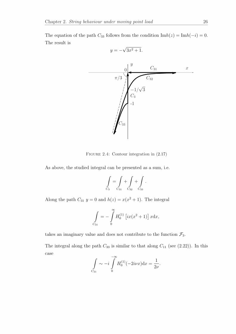
Chapter 2. String behaviour under moving point load 26
The equation of the path C33 follows from the condition Imh(z) = Imh(−i) = 0.
The result is
y = −√
3x2 + 1.
C3
C32
C33
C31 xy
−1/√
3
-1
π/3
0
Figure 2.4: Contour integration in (2.17)
As above, the studied integral can be presented as a sum, i.e.
∫
C3
=
∫
C31
+
∫
C32
+
∫
C33
.
Along the path C31 y = 0 and h(z) = x(x2 + 1). The integral
∫
C31
= −∞∫
0
H(1)0
[ix(x2 + 1)
]xdx,
takes an imaginary value and does not contribute to the function F3.
The integral along the path C33 is similar to that along C11 (see (2.22)). In this
case ∫
C31
∼ −i
−∞∫
0
H(1)0 (−2iνx)dx =
1
2ν.

Chapter 2. String behaviour under moving point load 27
Near the saddle point z2 = − i√3, one can derive from (2.28) y ≈ − 1√
3+ x,
z ≈ − i√3, dz ≈ (1 + i)dx and h(z) ≈ 2
√3x2 − 2
3√
3i. Hence,
∫
C32
∼ i
√2√
3
πνexp
(−i
2ν
3√
3
) +∞∫
−∞
e−2√
3νx2
dx,
and ∫
C3
∼ 1
ν
[1
2+ i exp
(−i
2ν
3√
3
)]. (2.29)
10 8 6 4 2 0 2 4 6 8 100
1
2
3
4
5
6
F1 F2
ϑ ϑ
Figure 2.5: The functions F1 and F2. Asymptotic functions (dashed lineand asterisk) and numerics (solid line).
0 1 2 3 4 5 6 7 8 9 10
−0.5
0.0
0.5
1.0
1.5
2.0
F3
ϑ
Figure 2.6: The function F3. Asymptotic functions (dashed line) and nu-merics (solid line).

Chapter 2. String behaviour under moving point load 28
ϑ F1 F2 F3 ϑ F1 F2 F3
0.0 1.04713 1.04713 0.00000 2.6 0.58912 0.11115 1.760450.1 1.01559 0.98280 0.10000 2.7 0.58088 0.09995 1.738270.2 0.98573 0.91931 0.19997 2.8 0.57263 0.08843 1.705620.3 0.95731 0.85697 0.29983 2.9 0.56431 0.07774 1.662500.4 0.93014 0.79721 0.39947 3.0 0.55592 0.06911 1.609060.5 0.90419 0.74135 0.49870 3.1 0.54759 0.06270 1.545540.6 0.87948 0.68948 0.59730 3.2 0.53947 0.05738 1.472320.7 0.85611 0.64039 0.69501 3.3 0.53174 0.05167 1.389930.8 0.83418 0.59273 0.79150 3.4 0.52454 0.04511 1.299010.9 0.81374 0.54625 0.88640 3.5 0.51796 0.03857 1.200371.0 0.79476 0.50200 0.97932 3.6 0.51197 0.03343 1.094921.1 0.77713 0.46135 1.06979 3.7 0.50648 0.03026 0.983721.2 0.76065 0.42469 1.15733 3.8 0.50131 0.02824 0.867961.3 0.74507 0.39101 1.24142 3.9 0.49626 0.02589 0.748911.4 0.73014 0.35877 1.32152 4.0 0.49116 0.02241 0.627981.5 0.71564 0.32725 1.39704 4.1 0.48587 0.01832 0.506631.6 0.70144 0.29713 1.46740 4.2 0.48036 0.01503 0.386421.7 0.68751 0.26977 1.53200 4.3 0.47467 0.01345 0.268931.8 0.67391 0.24590 1.59023 4.4 0.46893 0.01316 0.155761.9 0.66077 0.22483 1.64149 4.5 0.46332 0.01276 0.048522.0 0.64826 0.20502 1.68519 4.6 0.45802 0.01116 -0.051222.1 0.63651 0.18539 1.72079 4.7 0.45315 0.00852 -0.141952.2 0.62562 0.16623 1.74774 4.8 0.44880 0.00612 -0.222252.3 0.61556 0.14884 1.76558 4.9 0.44492 0.00515 -0.290822.4 0.60625 0.13423 1.77387 5.0 0.44142 0.00561 -0.346512.5 0.59751 0.12214 1.77225
Table 2.1: Tabulated values of canonical integrals
Substitution (2.29) into (2.17) leads to the formula
F3(ϑ) ∼ 1
ϑ1/2
(1 + 2 sin
(2ϑ3/2
3√
3
)). (2.30)
Further, we may expect that the canonical integrals (2.8), (2.10) and (2.12) de-
scribe the uniform asymptotic behaviour of more complicated integrals of this
type for the case in which the intermediate range ϑ ∼ 1 is also of interest.
The comparison of the asymptotic forms of the functions Fi (i = 1, 2, 3) with
the results of numerical computations for the integrals (2.8), (2.10) and (2.12)
is presented in Figures 2.5 and 2.6. Here and below the trapezium method with
10000-30000 points was used for numerical integration. The solid line in the first

Chapter 2. String behaviour under moving point load 29
and second quadrants of Figure 2.5 corresponds to the computed values of the
integrals (2.10) and (2.8), respectively. The asymptotic representations (2.23)
and (2.27) are plotted in this figure by the dashed line. In addition, the limiting
value (2.13) is denoted by an asterisk. In Figure 2.6 the results of the numerical
evaluation of the integral (2.12) (solid line) are shown with its asymptotic forms
(2.14) and (2.30) (dashed line). The tabulated values of the functions Fi are
also displayed in Table 2.1. Here and below all the numerical calculations were
performed in SciLab.
2.3 Constant acceleration case
Below we investigate the string behaviour at a moving point λ = 0, where a force
is applied, and also at a moving singularity λ = − (u−1)2
2, which is actually a shock
wave which appeared after the passage through the sound wave speed. This value
can be easily found (see details in [59]). The latter arises when passing through
the sound speed and coincides with a point λ = 0 at u = 1. The aforementioned
moving points are of most interest when investigating the passage through the
sound wave barrier. Here three combinations of the problem parameters are
studied.
2.3.1 The displacement under the load before the passage
(u ≤ 1 and λ = 0)
In this case the original integral in (2.3) becomes
I =
u∫
0
J0(νφ(u, 0, t))dt, (2.31)
with
φ(u, 0, t) = t
√1− u2 + t− t
[(1− u) +
t
4
]. (2.32)
In the vicinity of the end point t = 0 in the integral (2.31) one has φ(u, 0, t) ≈t√
1− u2, if t ¿ 1− u. Otherwise, for 1− u ¿ t ¿ 1 it appears that φ(u, 0, t) ≈

Chapter 2. String behaviour under moving point load 30
t3/2. The formula
φ(u, 0, t) ≈ t√
1− u2 + t, t ¿ 1, (2.33)
contains both of the limiting forms.
As above, to the leading order we can substitute infinity at the upper limit of the
last integral. Finally, the following simpler integral is obtained
I ∼∞∫
0
J0
(νt√
1− u2 + t)
dz. (2.34)
Next, changing the independent variable by t1 = tν2/3 we establish the sought
for uniform asymptotic behaviour in the parameters ν and u
I ∼ ν−2/3
∞∫
0
J0
(t1
√ν2/3(1− u2) + t1
)dt1, (2.35)
or
I ∼ ν−2/3F1(η), (2.36)
where the fundamental parameter η determines the scaling of the problem. It is
given by
η = ν2/3(1− u2). (2.37)
Outside the characteristic zone η ∼ 1 (1− u2 ∼ ν−2/3) the function F1 in (2.36)
can be reduced to the local forms (2.13) for η ¿ 1 (1 − u2 ¿ ν−2/3) and (2.23)
for η À 1 (1 − u2 À ν−2/3). Such an observation is relevant for other integrals
considered below in this section.
2.3.2 The displacement under the load after the passage
(u ≥ 1 and λ = 0)
Here
I =
u∫
2(u−1)
J0(νφ(u, 0, t))dt, (2.38)
with
φ(u, 0, t) =t
2
√(t− 2(u− 1))(2(u + 1)− t).

Chapter 2. String behaviour under moving point load 31
0.80 0.85 0.90 0.95 1.00 1.05 1.10 1.15 1.200
1
2
3
4
5
6
u
w(ν, 0, u)
ν = 100
ν = 50 `
ν = 10
0.90 0.92 0.94 0.96 0.98 1.00 1.02 1.04 1.06 1.08 1.100
2
4
6
8
10
12
u
w(ν, 0, u)
ν = 1000
ν = 500 `
ν = 250
Figure 2.7: Uniform asymptotic behaviour (solid line) and numerics (dashedline) of the function (2.3) using integrals (2.31) (u ≤ 1) and (2.36) (u ≥ 1).
In this case the function φ(u, 0, t) near the end point t = 2(u− 1) is presented as
φ(u, 0, t) ≈ t√
t− 2(u− 1). (2.39)
After changing the independent variable by
t1 = ν2/3(t− 2(u− 1)), (2.40)

Chapter 2. String behaviour under moving point load 32
it appears that
I ∼ ν−2/3
∞∫
0
J0
((t1 + 2ν2/3(u− 1))
√t1
)dt1 = ν−2/3F2(2ν
2/3(u− 1)). (2.41)
This asymptotic result is of interest only over the narrow vicinity of the sound
wave speed (u−1 ∼ ν−2/3) due to the exponential decay of the function F2. In this
case, the parameter η may be introduced in the last formula setting 2−u ≈ u2−1.
2.3.3 The displacement at the moving singularity
(u ≥ 1 and λ = −12(u− 1)2)
We have in (2.3)
I = I1 + I2, (2.42)
with
I1 =
u∫
u−1
J0
(νφ
(u,−1
2(u− 1)2, t
))dt, (2.43)
and
I2 =
u−1∫
(√
u−1)2
J0
(νφ
(u,−1
2(u− 1)2, t
))dt, (2.44)
where
φ
(u,−1
2(u− 1)2, t
)=
= ±(t− (u− 1))
√−1
4(t− (
√u− 1)2)(t− (
√u + 1)2). (2.45)
Here and below the signs ”+” and ”−” correspond to the integrals I1 and I2,
respectively.
The parameter range can be restricted by the values of u that are close enough
to the value u = 1. In this case√
u + 1 ≈ 2 may be set. Next, the function
(2.45) might be expanded near the left end point in the integral (2.43) and over
the whole integration domain in the integral (2.44). It becomes
φ
(u,−1
2(u− 1)2, t
)≈ ±(t− (u− 1))
√t− (
√u− 1)2.

Chapter 2. String behaviour under moving point load 33
1.00 1.05 1.10 1.15 1.20 1.25 1.30 1.35 1.400
2
4
6
8
10
12
u
w(ν,−1
2(u− 1)2, u
)
ν = 100
ν = 50
1.00 1.01 1.02 1.03 1.04 1.05 1.06 1.07 1.08 1.090
5
10
15
20
25
u
w(ν,−1
2(u− 1)2, u
)
ν = 1000
ν = 500
Figure 2.8: Uniform asymptotic behaviour (dashed line) and numerics (solidline) of the function (2.3) using integrals (2.42).
Now, change of the variables in the integrals (2.43) and (2.44) by the formula
t1 = ±ν2/3(t− (u− 1)) (2.46)
gives the result
I1 ∼ ν−2/3
∞∫
0
J0
(t1
√t1 + 2(
√u− 1)ν2/3
)dt1 =
= ν−2/3F1(2(√
u− 1)ν2/3),

Chapter 2. String behaviour under moving point load 34
and
I2 ∼ ν−2/3
2(√
u−1)ν2/3∫
0
J0
(t1
√2(√
u− 1)ν2/3 − t1
)dt1 =
= ν−2/3F3(2(√
u− 1)ν2/3).
Finally,
I ∼ ν−2/3[F1(2ν
2/3(√
u− 1)) + F3(2ν2/3(
√u− 1))
]. (2.47)
Similar to the previous case, we may operate with the functions Fj
(−12η)
(j =
1, 3) in the vicinity of the sound wave speed where√
u− 1 ≈ 14(u2 − 1).
2.3.4 Numerical results
The numerical examples are presented in Figures 2.7 and 2.8. In Figure 2.7 the
computed values of the function (2.3) are displayed using the formulae (2.31) and
(2.38) (dashed line) along with its uniform asymptotic behaviour given by the
formulae (2.36) and (2.41) (solid line). The graphs of the function (2.3) in case
of the integral (2.42) (dashed line) and the uniform asymptotic formula (2.47)
(solid line) are plotted in Figure 2.8.
These figures illustrate the uniform validity of the derived asymptotic formulae
in case of the moving load problem for a string. The striking difference between
the asymptotic behaviour of the functions F1 and F2 for ϑ À 1 leads to a strong
asymmetry of the transition curves in Figure 2.7. In Figure 2.8 the function
F3 reproduces the oscillatory patterns associated with the passage through the
sound wave barrier.
2.4 Constant deceleration case
Here we briefly describe an inverse transition through the sonic speed. In partic-
ular we would like to pay attention on a string behaviour under a moving load
just after the passage. In this case u ≤ 1 and λ = 0. Similar to the previous

Chapter 2. String behaviour under moving point load 35
section we obtain an integral:
w = ν
0∫
−2(1−u)
J0
(ν
√−1
4z2(z + 2(1− u))(z − 2(1 + u))
)dz. (2.48)
Since z ≈ 0 and u is in the vicinity of 1 then z − 2(1 + v1) ≈ −4 . Thus
w = ν
0∫
−2(1−u)
J0
(νz
√z + 2(1− u)
)dz.
Changing variables as z = ν−2/3y gives
w = ν1/3
0∫
−ν2/3(1−u)
J0
(y√
y + 2ν2/3(1− u)
)dy.
Introducing a new notation a = 2ν2/3(1− u) we obtain
w = ν1/3
0∫
−a
J0
(y√
y + a)dy.
Since J0 is an even function then substitution y = −t leads to
w = ν1/3
a∫
0
J0
(t√
a− t)dt = ν1/3F3(a) = ν1/3F3(2ν
2/3(1− u)). (2.49)
So, the derived asymptotic solution (2.49) is based on the function F3 introduced
above. As one can see in Figure 2.9 it provides a very close approximation (solid
line) to the exact integral solution (2.48) (dashed line) in the vicinity of sound
speed.
2.5 Arbitrary acceleration case
In this section we provide a draft of how to deal with the arbitrary acceleration
using the results for the constant one, which were obtained above. As an example

Chapter 2. String behaviour under moving point load 36
0.75 0.80 0.85 0.90 0.95 1.00
−5
0
5
10
15
20
ν = 1000
ν = 500
ν = 100ν = 10
u
w (ν, 0, u)
Figure 2.9: Asymptotic and numerical results for the integral (2.48).
we consider two possible paths: s(τ) = u0τ + ετ2
2and s(τ) = −A cos(ετ) (respec-
tive speeds are u(τ) = u0 +ετ and u(τ) = A sin(ετ)) (see Figure 2.10). Note that
the first path presents inverse transition from arbitrary to uniform acceleration
case.
Consider the general integral solution for the main problem (2.2) with a general
path function s1(τ) (not necessary equal to aτ2
2) in the right hand side of the
equation.
w =
τ∫
0
J0
(√ζ2 − (λ + s1(τ)− s1(τ − ζ))2
)σdζ. (2.50)
Here and below σ has the following behaviour:
σ =
{1, if ζ2 − (λ + s1(τ)− s1(τ − ζ))2 > 0;
0, if ζ2 − (λ + s1(τ)− s1(τ − ζ))2 < 0.
In the vicinity of ζ = 0, one can expand the path function s1 as
s1(τ − ζ) ≈ s1(τ)− u(τ)ζ +du
dτ
ζ2
2, ζ ¿ 1. (2.51)

Chapter 2. String behaviour under moving point load 37
u(τ) = u0 + ετ
u(τ)=Asin(ετ)u = 1
u
τ
kk
Figure 2.10: Transition through the sound wave barrier with constant accel-eration and sinusoidal speed function. The transition moment for each case is
shown by a circle
Substitution (2.51) into (2.50) leads to
w =
δ∫
0
J0
√ζ2 −
(λ + u(τ)ζ − du
dτ
ζ2
2
)2 σdζ. (2.52)
Assumption u = k(ετ) gives
w =
δ∫
0
J0
√ζ2 −
(λ + kζ − ε
dk
dτ
ζ2
2
)2 σdζ.
After the substitutions ζ =z
εit appears
w =1
ε
εδ∫
0
J0
1
ε
√z2 −
(ελ + kz − dk
dτ
z2
2
)2 σdz.

Chapter 2. String behaviour under moving point load 38
Now, assume that ν =1
εand λ1 = ελ =
λ
νand get
w = ν
δ/ν∫
0
J0
ν
√z2 −
(λ1 + kz − dk
dτ
z2
2
)2 σdz.
Consider the case when λ1 = 0:
w = ν
δ/ν∫
0
J0
ν
√z2 − k2z2 + k
dk
dτz3 −
(dk
dτ
)2z4
4
σdz.
Since the last term is a small value of the fourth order, it can be neglected and
we obtain the following formula
w = ν
δ/ν∫
0
J0
(ν
√z2(1− k2) + k
dk
dτz3
)σdz. (2.53)
Two cases with respect to values of k, namely, k < 1 and k > 1 (here k is assumed
to be in the vicinity of unity), should be considered:
(i) k < 1
Consider the (2.53) and assume that in the second term under a radical
sign k ≈ 1. In this case z2 dk
dτcan be moved from the square root sign and
w = ν
δ/ν∫
0
J0
(νz
√dk
dτ
√(1− k2)/
dk
dτ+ z
)dz.
Making a substitution z = y
(ν
√dk
dτ
)−2/3
and also assuming that the
upper limit in integral is going towards ∞, one may get
w = ν1/3
(dk
dτ
)−1/3∞∫
0
J0
y
√(1− k2)ν2/3
(dk
dτ
)−2/3
+ y
dy,
or
w = ν1/3
(dk
dτ
)−1/3
F1
((1− k2)ν2/3
(dk
dτ
)).

Chapter 2. String behaviour under moving point load 39
(ii) k > 1
By analogy with the previous case, we consider the integral (2.53), but
here the lower limit is changed because the phase function should be non-
negative on the entire interval of integration.
w = ν
δ/ν∫
2(k−1)dk
dτ
4/3
J0
νz
√dk
dτ
√√√√z − k2 − 1
dk
dτ
dz.
Substitution z = y
(ν
√dk
dτ
)−2/3
and the assumption that the upper inte-
gration limit is going towards ∞ imply that
w = ν1/3
(dk
dτ
)−1/3
×
×∞∫
2(k−1)ν2/3
dk
dτ
4/3
J0
y
√y − (k2 − 1)ν2/3
(dk
dτ
)−2/3 dy.
Now, assume that k2 − 1 ≈ 2(k − 1) and make the substitution x = y −(k2 − 1)ν2/3
(dk
dτ
)−2/3
. The result is
w = ν1/3
(dk
dτ
)−1/3∞∫
0
J0
(√
x
(x + 2(k − 1)ν2/3
(dk
dτ
)−2/3))
dx,
or
w = ν1/3
(dk
dτ
)−1/3
F2
(2(k − 1)ν2/3
(dk
dτ
)−2/3)
.
So, the general case asymptotic forms are:
w = ν1/3
(dk
dτ
)−1/3
F1
((1− k2)ν2/3
(dk
dτ
)), (k < 1)

Chapter 2. String behaviour under moving point load 40
and
w = ν1/3
(dk
dτ
)−1/3
F2
(2(k − 1)ν2/3
(dk
dτ
)−2/3)
, (k > 1).
It remains to substitute the example paths into the latter formulae.
(i) k = ετ = v
Thus, ∂k∂τ
= 1 and it leads to
w = ν1/3F1
((1− v2)ν2/3
), (k < 1)
and
w = ν1/3F2
(2(v − 1)ν2/3
), (k > 1).
Here we note that these results are exactly the same as the ones given in
Section 2.3, but here they are obtained for a more general case.
(ii) k = A sin(ετ)
Assume that ν = 1ε
and k ≈ 1 (so ∂k∂τ
= A cos(ετ) = A√
1− sin2(ετ) =√A2 − 1). In this case
w =(ε√
A2 − 1)−1/3
F1
(1− A2 sin2(ετ)(ε√
A2 − 1)2/3
), (k < 1) (2.54)
and
w =(ε√
A2 − 1)−1/3
F2
(2 (A sin(ετ)− 1)(ε√
A2 − 1)2/3
), (k > 1). (2.55)
The graphs given in Figures 2.11–2.13 geometrically describe the exact and
asymptotic solutions for the different values of the parameters A and ν.
Comparing these figures one can notice that the derived formulae (2.54)
– (2.55) provide a better approximation for integral solution (2.50) when
parameter ν is sufficiently large and parameter A is close to the unity (note
that A can not be less or equal to 1, otherwise there is no passage through
the critical speed), i.e. when the transition is quite slow. As you can see,
there are some local corners and roughness (especially sufficiently far from
critical speed) on the lines on the figures. These features appear because
of some local errors in numerical integration.

Chapter 2. String behaviour under moving point load 41
4
5
3
0.950.90
6
2
1.05
0
1
1.00 1.10
7
8
9
-1
A = 1.1
A = 3
A = 9
u
w
Figure 2.11: The exact solution (2.50) (dashed line) along with the asymp-totic solution (2.54)–(2.55) (solid line) under the load for ν = 250
2.6 Special asymptotic forms
2.6.1 Steady speed asymptotic behaviour near the load
case
Again, consider (2.50) and the series (2.51), but now only the first two terms of
the series are the object of the attention, due to the fact that the speed is steady,
or zero acceleration. So,
w =
δ∫
0
J0
(√ζ2 − (λ + uζ)2
)σdζ,
or after some transformations of the phase function
w =
δ∫
0
J0
(√(1− u2)
(ζ − λ
1− u
)(ζ +
λ
1 + u
))σdζ.

Chapter 2. String behaviour under moving point load 42
4
5
3
0.950.90
6
2
1.05
0
1
1.00 1.10
7
-1
A = 1.1
A = 3
A = 9
u
w
Figure 2.12: The exact solution (2.50) (dashed line) along with the asymp-totic solution (2.54)–(2.55) (solid line) under the load for ν = 100
The roots of the phase function are
T0 =λ
1− u; T1 =
λ
1 + u, (T0 > T1).
Now one can make a substitution
p = ζ − Ti, (i = 0 if λ > 0; i = 1 if λ < 0).
So now there are two cases of λ values for the case of u < 1:
(i) λ > 0
In this case
w =
δ−T0∫
0
J0
(√(1− u2) p
(p +
2λ
1− u2
))dp.
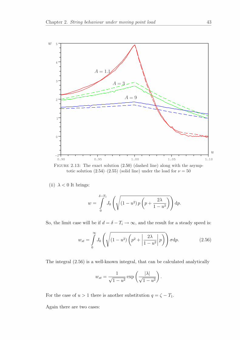
Chapter 2. String behaviour under moving point load 43
4
5
3
0.950.90
-1
2
1.05
0
1
1.00 1.10
A = 1.1
A = 3
A = 9
u
w
Figure 2.13: The exact solution (2.50) (dashed line) along with the asymp-totic solution (2.54)–(2.55) (solid line) under the load for ν = 50
(ii) λ < 0 It brings:
w =
δ−T1∫
0
J0
(√(1− u2) p
(p +
2λ
1− u2
))dp.
So, the limit case will be if d = δ− Ti →∞, and the result for a steady speed is:
wst =
∞∫
0
J0
(√(1− u2)
(p2 +
∣∣∣∣2λ
1− u2
∣∣∣∣ p
))σdp. (2.56)
The integral (2.56) is a well-known integral, that can be calculated analytically
wst =1√
1− u2exp
( |λ|√1− u2
).
For the case of u > 1 there is another substitution q = ζ − T1.
Again there are two cases:

Chapter 2. String behaviour under moving point load 44
λ
w
Figure 2.14: The exact solution (solid line) along with the static speed solu-tion (dashed line) for u < 1 (u = 0.8).
(i) T1 < τ < T0
In other words, the above mentioned substitution gives 0 < d < 2λ1−u2 = 2γ.
And the integral transforms into
w =
τ∫
T1
J0
(√(1− u2)q (q + T1 − T0)
)dq =
=
a∫
0
J0
(√(u2 − 1) (−q2 + 2γq)
)dq.
(ii) τ > T0
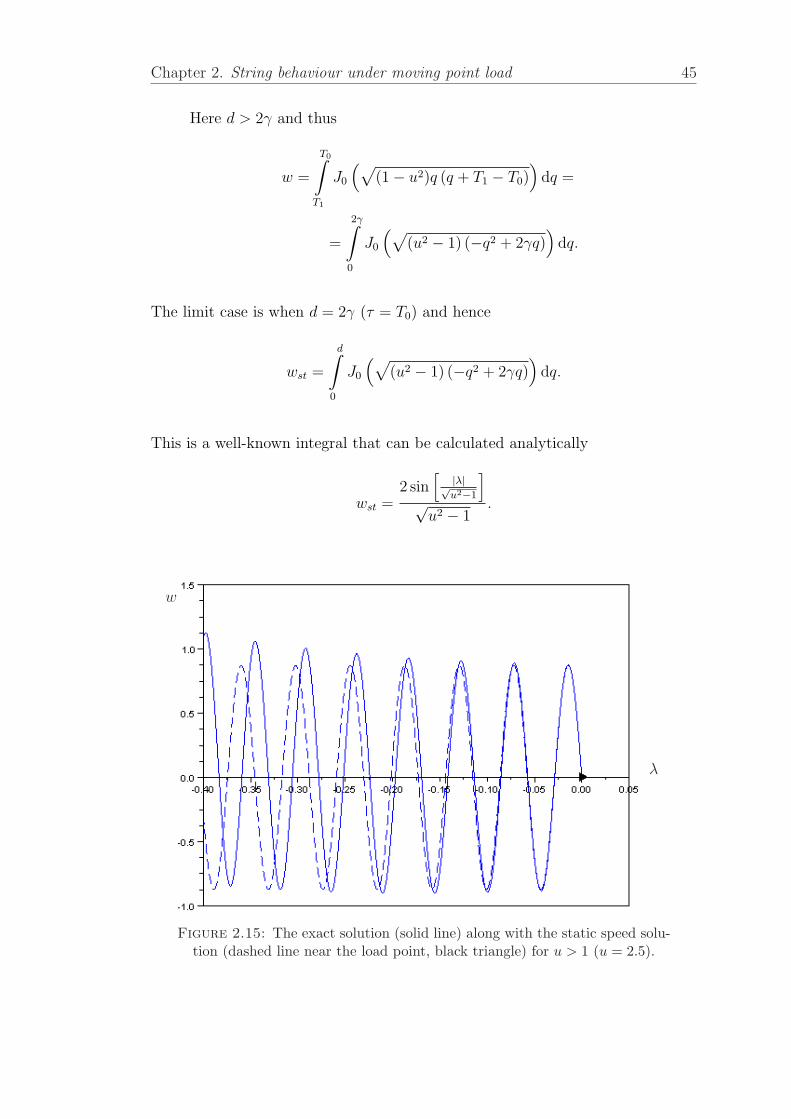
Chapter 2. String behaviour under moving point load 45
Here d > 2γ and thus
w =
T0∫
T1
J0
(√(1− u2)q (q + T1 − T0)
)dq =
=
2γ∫
0
J0
(√(u2 − 1) (−q2 + 2γq)
)dq.
The limit case is when d = 2γ (τ = T0) and hence
wst =
d∫
0
J0
(√(u2 − 1) (−q2 + 2γq)
)dq.
This is a well-known integral that can be calculated analytically
wst =2 sin
[|λ|√u2−1
]√
u2 − 1.
λ
w
Figure 2.15: The exact solution (solid line) along with the static speed solu-tion (dashed line near the load point, black triangle) for u > 1 (u = 2.5).

Chapter 2. String behaviour under moving point load 46
2.6.2 Asymptotic behaviour near singularity area
Here the stationary points are considered, one for the area in front of the shock
wave and two of them beyond the shock wave. This section contains only the con-
stant positive acceleration case, because it is too hard to find such an asymptotic
representations for more complicated cases.
Figure 2.16: Evolution of the phase function (expression under square rootsin (2.57)) against z for the different values of λ for u = 2.5
So, consider the following integral:
I =
u∫
0
J0
ν
√z2 −
(λ1 + uz − 1
2z2
)2 dz. (2.57)
We need to find the contribution of all stationary points by the classic stationary
phase method. For this, first we have to transfer the Bessel function in the
integral (2.57) to its asymptotic formula with an exponential function, as follows
J0(ν√
Φ(z)) ≈√
2
πΦ(z)Re exp
(Φ(z)− π
4
). (2.58)

Chapter 2. String behaviour under moving point load 47
Now one may use the stationary phase method. To do so one or two (depending on
the value of λ, see Figure 2.16) stationary points should be found. It is impossible
to make it analytically, due to the complicated nature of the phase function. So,
it was done by numerical methods. After finding these phase points, it remains
to substitute the results into the following formula
I1,2 =
√2π
ν|Φ′′(z0)|f(z0) cos(ν√
Φ(z0)− π
4+
π
4sgn (Φ′′(z0))
),
where Φ is a phase function, f(z) - is a term, staying before exp in the (2.58), z0
is a stationary point, calculated numerically.
The final step is to find a sum of contributions of all the stationary points. This
will tend to the asymptotic result (see Figures 2.15 and 2.17), that works near
the shock wave (λ3, red diamond) and at the end of singularity area (λ4, green
diamond).
λ
w
Figure 2.17: The exact solution (solid line) and static speed solution withcontributions from stationary points of phase function (dashed line) for u > 1
(u = 2.5).

Chapter 2. String behaviour under moving point load 48
2.7 Summary
In this chapter we investigated the asymptotic behaviour of an elastically sup-
ported infinite string under a moving point load.
The auxiliary canonical functions Fi, i = 1, 2, 3, were introduced, asymptotically
analyzed and tabulated in Section 2.2. Using these functions the uniform asymp-
totic formulae for a string under the constant accelerating and decelerating point
loads were obtained in Sections 2.3 and 2.4 respectively.
The asymptotic formulae for an arbitrary acceleration case were presented and
then applied for the case of sinusoidal load speed u(τ) = A sin(ετ) in Section 2.5.
It was shown that the canonical functions Fi, i = 1, 2, 3, can successfully be used
in an arbitrary acceleration case as well.
In Section 2.6 we obtained the approximate formulae for the vicinity of point load
and singularity area behind the shock wave using the steady speed asymptotic
expansion with the additional contributions from the stationary points where
appropriate.

Chapter 3
Vibrations of an infinite half
plane under moving point load
3.1 Statement of the problem
The main object of consideration is an elastic isotropic infinite half plane (−∞ <
x < ∞, 0 ≤ y < ∞) subject to a point load (line load for three dimensional case)
of an amplitude P0 moving along the surface y = 0 with a constant acceleration
a (see Figure 3.1).
We start with the asymptotic model which was suggested in [61] and describes
the half plane behaviour for the load speeds close to the Rayleigh wave speed.
In doing so, the model ignores the bulk compression and shear waves, which
appear in general Lame equation for the half plane. The horizontal and vertical
displacements u1 and u2 can be expressed in terms of the Lame potentials φ and
ψ (in frames of general elastic theory):
u1 = φx − ψy, u2 = φy + ψx. (3.1)
Here and below subscripts x and y denote the partial derivatives ∂∂x
and ∂∂y
.
Further on we will use both of these notations.
The elliptic equations for the interior field in the above mentioned model can be
expressed in the form
φyy + k21φxx = 0, ψyy + k2
2ψxx = 0, (3.2)
49

Chapter 3. Vibrations of infinite half plane 50
P0
at
x
y
Figure 3.1: Elastic isotropic infinite half plane subject to a moving pointload
where
k2i = 1− c2
R
c2i
, (i = 1, 2), (3.3)
and
(1 + k22)
2 = 4k1k2. (3.4)
The formula (3.4), using expression (3.3), can be written as the classic Rayleigh
equation:
4
√1− c2
R
c21
√1− c2
R
c22
−(
2− c2R
c22
)2
= 0
and, thus, gives the dependence between cR and the Poisson ratio, which is coming
from the bulk wave speeds c1 and c2.
Here cR denotes the Rayleigh wave speed, c1 and c2 are the longitudinal and shear
wave speeds, respectively.
At the surface y = 0 we have the following boundary conditions
φxx(x, 0, t)− c−2R φtt(x, 0, t) = AP0δ
(x− 1
2at2
)(3.5)
and
− 2
1 + k22
φy(x, 0, t) = ψx(x, 0, t). (3.6)
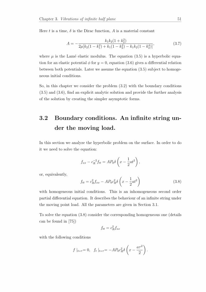
Chapter 3. Vibrations of infinite half plane 51
Here t is a time, δ is the Dirac function, A is a material constant
A = − k1k2(1 + k22)
2µ[k2(1− k21) + k1(1− k2
2)− k1k2(1− k42)]
, (3.7)
where µ is the Lame elastic modulus. The equation (3.5) is a hyperbolic equa-
tion for an elastic potential φ for y = 0, equation (3.6) gives a differential relation
between both potentials. Later we assume the equation (3.5) subject to homoge-
neous initial conditions.
So, in this chapter we consider the problem (3.2) with the boundary conditions
(3.5) and (3.6), find an explicit analytic solution and provide the further analysis
of the solution by creating the simpler asymptotic forms.
3.2 Boundary conditions. An infinite string un-
der the moving load.
In this section we analyze the hyperbolic problem on the surface. In order to do
it we need to solve the equation:
fxx − c−2R ftt = AP0δ
(x− 1
2at2
),
or, equivalently,
ftt = c2Rfxx − AP0c
2Rδ
(x− 1
2at2
)(3.8)
with homogeneous initial conditions. This is an inhomogeneous second order
partial differential equation. It describes the behaviour of an infinite string under
the moving point load. All the parameters are given in Section 3.1.
To solve the equation (3.8) consider the corresponding homogeneous one (details
can be found in [75])
ftt = c2Rfxx
with the following conditions
f |t=τ= 0, ft |t=τ= −AP0c2Rδ
(x− aτ 2
2
).

Chapter 3. Vibrations of infinite half plane 52
The solution to the homogeneous equation has a form
f(x, t) = −AP0cR
2
t∫
0
x+cR(t−τ)∫
x−cR(t−τ)
δ
(ξ − aτ 2
2
)dξ
dτ.
The result of the inner integration is the Heaviside function denoted as H. Hence,
f(x, t) = −AP0cR
2
t∫
0
[H
(x + cR(t− τ)− aτ 2
2
)−H
(x− cR(t− τ)− aτ 2
2
)]dτ.
λ
φ
λ2λ1
Figure 3.2: Boundary condition for v = 0.95 (λ1 = −1.40125, λ2 = 0.49875)
Introducing a moving coordinate system: (s, t) =(x− at2
2, t
)and changing vari-
able r = t− τ give
f(s, t) =AP0cR
2
t∫
0
[H
(s + r(at + cR)− ar2
2
)−
−H
(s + r(at− cR)− ar2
2
)]dr. (3.9)
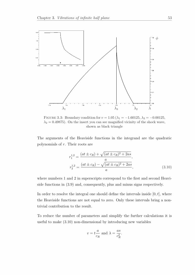
Chapter 3. Vibrations of infinite half plane 53
λ
φ
λ2λ3λ1
Figure 3.3: Boundary condition for v = 1.05 (λ1 = −1.60125, λ3 = −0.00125,λ2 = 0.49875). On the insert you can see magnified vicinity of the shock wave,
shown as black triangle
The arguments of the Heaviside functions in the integrand are the quadratic
polynomials of r. Their roots are
r1,21 =
(at± cR) +√
(at± cR)2 + 2as
a,
r1,22 =
(at± cR)−√
(at± cR)2 + 2as
a, (3.10)
where numbers 1 and 2 in superscripts correspond to the first and second Heavi-
side functions in (3.9) and, consequently, plus and minus signs respectively.
In order to resolve the integral one should define the intervals inside [0, t], where
the Heaviside functions are not equal to zero. Only these intervals bring a non-
trivial contribution to the result.
To reduce the number of parameters and simplify the further calculations it is
useful to make (3.10) non-dimensional by introducing new variables
v = ta
cR
and λ =as
c2R
.

Chapter 3. Vibrations of infinite half plane 54
In this case the roots (3.10) can be written as
ρ1,21 = (v ± 1) +
√(v ± 1)2 + 2λ,
ρ1,22 = (v ± 1)−
√(v ± 1)2 + 2λ,
where upper indices 1 and 2 correspond to the plus and minus signs respectively.
Note that ρ1,22 < ρ1,2
1 .
To define the intervals mentioned above it is sufficient to consider the following
cases
(i) 0 < ρ1,22 < v; 0 < ρ1,2
1 < v: the length of the interval is ρ1,21 − ρ1,2
2 .
(ii) ρ1,22 < 0; 0 < ρ1,2
1 < v: the length of the interval is ρ1,21 .
(iii) 0 < ρ1,22 < v; ρ1,2
1 > v: the length of the interval is v − ρ1,22 .
(iv) ρ1,22 < 0; ρ1,2
1 > v: the length of the interval is v.
These cases should be considered for v ≤ 1, 1 ≤ v ≤ 2 and v ≥ 2.
To classify the roots we use the notation
λ1 =1− (1 + v)2
2, λ2 =
1− (1− v)2
2, λ3 = −(1− v)2
2,
s1 =c2R − (cR + at)2
2a, s2 =
c2R − (cR − at)2
2a, s3 = −(cR − at)2
2a.
The results (for non-dimensional variables along with dimensional ones) obtained
via straightforward calculations are presented in the Table 3.1.
Remark: Further on in this thesis we consider only the data displayed in the first
and second columns of Table 3.1 (see Figures 3.2 and 3.3 respectively), because
our main object of interest is the vicinity of the transition through the Rayleigh
speed. Note also that the model, described in this work, does not involve the
passage through the sonic speed. So, the results obtained within the framework
of this model do not describe adequately the real behaviour of a half plane in
case when the velocity of the load is greater than the sound wave speed.

Chapter 3. Vibrations of infinite half plane 55
t≤
c R a(v≤
1)c R a≤
t≤
2cR a
(1≤
v≤
2)t≥
2cR a
(v≥
2)
For
s 1≤
s≤
0(λ
1≤
λ≤
0):
For
0≤
s≤
s 2(0≤
λ≤
λ2):
For
s 2≤
s≤
0(λ
1≤
λ≤
λ3):
f=
AP
0c2 R
2a(v−
ρ1 2)
=A
P0c R
2
( t−
r1 2
)f
=A
P0c2 R
2a(v−
ρ2 1)
=A
P0c R
2(t−
r2 1)
f=
AP
0c2 R
2a(v−
ρ1 2)
=A
P0c R
2(r
2 2−
r1 2)
For
0≤
s≤
s 2(0≤
λ≤
λ2):
For
s 3≤
s≤
0(λ
3≤
λ≤
0):
For
s 3≤
s≤
s 2(λ
3≤
λ≤
λ2):
f=
AP
0c2 R
2a(v−
ρ2 1)
=A
P0c R
2
( t−
r2 1
)f
=A
P0c2 R
2a(v−
ρ2 1−
(ρ1 2−
ρ2 2))
=f
=A
P0c2 R
2a(v−
ρ1 2−
(ρ2 1−
ρ2 2))
=
=A
P0c R
2(t−
r2 1+
r2 2−
r1 2)
=A
P0c R
2(t−
r2 1+
r2 2−
r1 2)
For
s 1≤
s≤
s 3(λ
1≤
λ≤
λ3):
For
s 1≤
s≤
s 3(λ
2≤
λ≤
0):
f=
AP
0c2 R
2a(v−
ρ1 2)
=A
P0c R
2(t−
r1 2)
f=
AP
0c2 R
2a(ρ
2 2−
ρ1 2)
=A
P0c R
2(r
2 2−
r1 2)
Table
3.1
:C
lass
ifica
tion
ofth
ero
ots

Chapter 3. Vibrations of infinite half plane 56
3.3 The exact solution over the interior
First of all, it is necessary to state again, that the term ”exact solution” does
not mean exact solution within the framework of the general theory of elasticity,
but only the solution within the framework of the asymptotic model (see [61])
without any additional assumptions and approximations.
This section is dedicated to the calculation of the displacements (3.1). In order to
do that we need to find the Lame potentials φ and ψ by resolving the equations
(3.2) with the boundary conditions (3.5) and (3.6).
Two speed intervals at ≤ cR and at ≥ cR are considered separately and the
corresponding results are given below.
3.3.1 Before the passage
Start with the equation (3.2) for the potential φ, rewritten in the variables y and
s:
φyy + k21φss = 0 (3.11)
with the boundary condition, obtained in Section 3.2
φ(s, 0, t) = f(s, t) =
AP0cR
2
(t− r1
2
), for s1 ≤ s ≤ 0;
AP0cR
2
(t− r2
1
), for 0 ≤ s ≤ s2;
0, otherwise.
(3.12)
The associated fundamental solution Φ(x, y) of the boundary-value problem
Φyy + k21Φxx = 0, Φ(x, 0) = δ(x)
is
Φ(x, y) =k1y
π(x2 + (k1y)2). (3.13)

Chapter 3. Vibrations of infinite half plane 57
Then the solution for the potential φ(s, y, t) can be found as a convolution of
(3.13) and (3.12) (details can be found in [75]):
φ(s, y, t) =
∞∫
−∞
φ(r, 0, t)Φ(s− r, y)dr =1
π
s2∫
s1
k1y
(r − s)2 + k21y
2φ(r, 0, t)dr
Integration by parts gives
φ(s, y, t) = − 1
π
s2∫
s1
arctan
(r − s
k1y
)∂φ(r, 0, t)
∂rdr. (3.14)
Partial derivative of the potential φ(r, y, t) with respect to r at y = 0 is
∂φ
∂r(r, 0, t) =
AP0cR
21√
(cR+at)2+2ar, for s1 < r < 0;
−AP0cR
21√
(cR−at)2+2ar, for 0 < r < s2.
(3.15)
Since the boundary condition (3.12) and, consequently, the partial derivative
(3.15) are different for the intervals s1 ≤ s ≤ 0 and 0 ≤ s ≤ s2, then the integral
(3.14) can be written as:
φ(s, y, t) = −AP0cR
2π(I1 − I2) ,
where
I1 =
0∫
s1
arctan(
r−sk1y
)√
(cR + at)2 + 2ardr; I2 =
s2∫
0
arctan(
r−sk1y
)√
(cR − at)2 + 2ardr. (3.16)
First, we calculate the integral I1. After an elementary transformation it can be
written in the form
I1 =1√2a
0∫
s1
arctan(
r−sk1y
)√
r +(
cR+at√2a
)2dr.

Chapter 3. Vibrations of infinite half plane 58
Applying integration by parts with
u = arctan
(r − s
k1y
), du =
1
k1y
1
1 +(
r−sk1y
)2 dr;
v = 2
√r +
(cR + at√
2a
)2
, dv =1√
r +(
cR+at√2a
)2dr,
one can obtain
I1 =1√2a
2
√r +
(cR + at√
2a
)2
arctan
(r − s
k1y
)
0
s1
− I ,
where
I =1
k1y
0∫
s1
2
√r +
(cR+at√
2a
)2
1 +(
r−sk1y
)2 dr.
To simplify the calculation of I let us introduce the change of variables
z =
√r +
(cR + at√
2a
)2
.
Then,
r = z2 −(
cR + at√2a
)2
, dr = 2zdz,
and the limits of integration are:
cR√2a
,cR + at√
2a.
Hence,
I = k1y
cR+at√2a∫
cR√2a
4z2dz
z4 − 2z2b1 + b21 + (k1y)2
,
where b1 =(cR + at)2
2a+ s.

Chapter 3. Vibrations of infinite half plane 59
Factorizing the denominator and applying partial fractions to the integrand, one
can get:
I = k1y
cR+at√2a∫
cR√2a
[2z√
2b1+2α1
z2 −√2b1 + 2α1z + α1
−2z√
2b1+2α1
z2 +√
2b1 + 2α1z + α1
]dz,
where α1 =√
b21 + (k1y)2.
The further transformations of I are
I =k1y√
2b1 + 2α1
cR+at√2a∫
cR√2a
2z −√2b1 + 2α1 +√
2b1 + 2α1
z2 −√2b1 + 2α1z + α1
dz−
−
cR+at√2a∫
cR√2a
2z +√
2b1 + 2α1 −√
2b1 + 2α1
z2 +√
2b1 + 2α1z + α1
dz
=
=k1y√
2b1 + 2α1
lnz2 −√2b1 + 2α1z + α1
z2 +√
2b1 + 2α1z + α1
∣∣∣∣cR+at√
2acR√2a
+
+ k1y
cR+at√2a∫
cR√2a
dz(z −
√2b1+2α1
2
)2
+(α1 − 2b1+2α1
4
) +
+ k1y
cR+at√2a∫
cR√2a
dz(z +
√2b1+2α1
2
)2
+(α1 − 2b1+2α1
4
) =
=
[k1y√
2b1 + 2α1
lnz2 −√2b1 + 2α1z + α1
z2 +√
2b1 + 2α1z + α1
+
+2k1y√
2α1 − 2b1
(arctan
z −√
2b1+2α1
2√2α1−2b1
2
+ arctanz +
√2b1+2α1
2√2α1−2b1
2
)] ∣∣∣∣cR+at√
2acR√2a
.
Finally,
I1 =1√2a
[ξ1(s, y, z2)− ξ1(s, y, z1)],

Chapter 3. Vibrations of infinite half plane 60
where
ξ1(s, y, z) = 2z arctanz2 − b1
k1y− k1y
β1
lnz2 − β1z + α1
z2 + β1z + α1
−
−2k1y
γ1
[arctan
2z − β1
γ1
+ arctan2z + β1
γ1
], (3.17)
z1 =cR√2a
, z2 =cR + at√
2a
and
b1 =(at + cR)2
2a+ s, α1 =
√b21 + (k1y)2,
β1 =√
2α1 + 2b1, γ1 =√
2α1 − 2b1. (3.18)
The integral I2 can be calculated in exactly the same way. The result is:
I2 =1√2a
[ξ2(s, y, z4)− ξ2(s, y, z3)],
where
ξ2(s, y, z) = 2z arctanz2 − b2
k1y− k1y
β2
lnz2 − β2z + α2
z2 + β2z + α2
−
−2k1y
γ2
[arctan
2z − β2
γ2
+ arctan2z + β2
γ2
], (3.19)
z3 =cR − at√
2a, z4 =
cR√2a
,
and
b2 =(cR − at)2
2a+ s, α2 =
√b22 + (k1y)2,
β2 =√
2b2 + 2α2, γ2 =√
2α2 − 2b2. (3.20)
Hence, the potential φ(s, y, t) for cR ≥ at is
φ(s, y, t) =AP0cR
2π√
2a[ξ1(s, y, z2)− ξ1(s, y, z1) + ξ2(s, y, z3)− ξ2(s, y, z4)]. (3.21)
To calculate the potential ψ one needs to solve the second equation in (3.2) with
the boundary condition (3.6). In order to use this boundary condition, the partial

Chapter 3. Vibrations of infinite half plane 61
derivative∂φ
∂yshould be calculated. To simplify this operation, one can use the
notation:
bi =1
2ab′i, αi =
1
2aα′i, βi =
1√2a
β′i, γi =1√2a
γ′i, i = 1, 2,
zj =1√2a
z′j, j = 1, 2, 3, 4,
ξi(s, y, z) =√
2aξ′i(s, y, z), i = 1, 2,
where
b′i = (cR ± at)2 + 2as, α′i =√
(b′1)2 + (2ak1y)2, i = 1, 2,
β′i =√
2(b′1 + α′1), γ′i =√
2(α′1 − b′1), i = 1, 2,
z′1 = z′4 = cR, z′2 = (cR + at), z′3 = (cR − at)
and
ξ′i(s, y, z′) =1
az′ arctan
(z′)2 − b′i2ak1y
− k1y
β′iln
(z′)2 − β′iz′ + α′i
(z′)2 + β′iz′ + α′i−
−2k1y
γ′i
[arctan
2z′ − β′iγ′i
+ arctan2z′ + β′i
γ′i
], i = 1, 2.
Here and below we use the notation without dashes but keep in mind that all the
parameters are defined as the ”dashed” ones above.
Partial derivative of the potential φ can be obtained straightforward. Performing
the massive (but relatively simple) calculations one can get:
∂φ
∂y(s, y, t) =
ϑ
π
[∂ξ1
∂y(z=cR+at)− ∂ξ1
∂y(z=cR)+
∂ξ2
∂y(z=cR−at)− ∂ξ2
∂y(z=cR)
].
where
∂ξi
∂y= −k1
[(1
βi
− f 2y2
αiβ3i
)ln
z2 − βiz + αi
z2 + βiz + αi
+
+ 2
(1
γi
− f 2y2
αiγ3i
)(arctan
2z − βi
γi
+ arctan2z + βi
γi
)]. (3.22)
Here and below f = 2ak1, ϑ = AP0cR
2.
Chapter 3. Vibrations of infinite half plane 62
For the sake of simplicity one can rewrite (3.22) as
∂ξi
∂y= −k1
[βi
4αi
lnz2 − βiz + αi
z2 + βiz + αi
+γi
2αi
(arctan
2z − βi
γi
+ arctan2z + βi
γi
)],
using the equalities
1
βi
− f 2y2
αiβ3i
=βi
4αi
,1
γi
− f 2y2
αiγ3i
=γi
4αi
.
Note that both equations in (3.2) have the same form, the only difference is in the
coefficient for∂2
∂s2. Hence, using the boundary condition (3.6), we can state that
the partial derivatives∂ψ
∂s(s, y, t) and
∂φ
∂y(s, y, t) are different only in a constant
coefficient − 21+k2
2. So, partial derivative of the potential ψ is
∂ψ
∂s(s, y, t) =
2ϑk1
(1 + k22)π
[∂ζ1
∂s(z = cR + at)− ∂ζ1
∂s(z = cR)+
+∂ζ2
∂s(z = cR − at)− ∂ζ2
∂s(z = cR)
],
where
∂ζi
∂s=
βi
4αi
lnz2 − βiz + αi
z2 + βiz + αi
+γi
2αi
[arctan
2z − βi
γi
+ arctan2z + βi
γi
]. (3.23)
Here and below αi, βi, γi are the same as αi, βi, γi, but with k2 instead of k1
in their definitions. This distinction comes from the different coefficients in the
equations (3.2).
Note that∂
∂s
(βi
4a
)=
βi
4αi
,∂
∂s
(γi
2a
)= − γi
2αi
,
hence, by integrating (3.23), one can obtain:
ζi =βi
4aln
z2 − βiz + αi
z2 + βiz + αi
− γi
2a
[arctan
2z − βi
γi
+ arctan2z + βi
γi
]+ F. (3.24)
To complete the calculation of the potential ψ, it remains to find explicitly the
function F in (3.24). If one compares the formulae (3.23) and (3.24) it becomes

Chapter 3. Vibrations of infinite half plane 63
clear that the partial derivative of F has a form:
∂F
∂s= − 2z(bi − z2)
(bi − z2)2 + f 2y2,
consequently,
F = − z
2aln
(bi − z2)2 + f 2y2
B.
The quantity B is an arbitrary element and does not depend on s. Since the
argument of the logarithm should be non-dimensional, one can put B = c4R.
Then,
F = − z
2aln
(bi − z2)2 + f 2y2
c4R
and the formula (3.24) transforms to
ζi =βi
4aln
z2 − βiz + αi
z2 + βiz + αi
− γi
2a
[arctan
2z − βi
γi
+ arctan2z + βi
γi
]−
− z
2aln
(bi − z2)2 + f 2y2
c4R
. (3.25)
With respect to (3.25), the potential ψ has a form
ψ(s, y, t) =2AP0cR
2π
k1
1 + k22
[ζ1(z = cR + at)− ζ1(z = cR)+
+ ζ2(z = cR − at)− ζ2(z = cR)] . (3.26)
It remains to calculate explicitly the displacements (3.1). We remind that (s, t) =
(x − 12at2, t), it means that the partial derivative with respect to s can be used
instead of∂
∂x.
So, the derivatives of the potentials φ and ψ are
∂φ
∂s=
AP0cR
2π
[∂ξ1
∂s(z = cR + at)− ∂ξ1
∂s(z = cR)+
+∂ξ2
∂s(z = cR − at)− ∂ξ2
∂s(z = cR)
], (3.27)
where
∂ξi
∂s=
ak1y
αiβi
lnz2 − βiz + αi
z2 + βiz + αi
− 2ak1y
αiγi
[arctan
2z − βi
γi
+ arctan2z + βi
γi
];

Chapter 3. Vibrations of infinite half plane 64
∂φ
∂y=
AP0cR
2π
[∂ξ1
∂y(z = cR + at)− ∂ξ1
∂y(z = cR)+
+∂ξ2
∂y(z = cR − at)− ∂ξ2
∂y(z = cR)
], (3.28)
where
∂ξi
∂y= −k1
[βi
4αi
lnz2 − βiz + αi
z2 + βiz + αi
+γi
2αi
(arctan
2z − βi
γi
+ arctan2z + βi
γi
)];
∂ψ
∂s=
2AP0cR
2π
k1
1 + k22
[∂ζ1
∂s(z = cR + at)− ∂ζ1
∂s(z = cR)+
+∂ζ2
∂s(z = cR − at)− ∂ζ2
∂y(z = cR)
], (3.29)
where
∂ζi
∂s=
βi
4αi
lnz2 − βiz + αi
z2 + βiz + αi
+γi
2αi
[arctan
2z − βi
γi
+ arctan2z + βi
γi
];
∂ψ
∂y=
AP0cR
2π
k1
1 + k22
[∂ζ1
∂y(z = cR + at)− ∂ζ1
∂y(z = cR)+
+∂ζ2
∂y(z = cR − at)− ∂ζ2
∂y(z = cR)
], (3.30)
where
∂ζi
∂y=
f 2y
4aαiβi
lnz2 − βiz + αi
z2 + βiz + αi
− f 2y
2aαiγi
[arctan
2z − βi
γi
+ arctan2z + βi
γi
].
The last step is to substitute the formulae (3.27)–(3.30) into (3.1). The result is:
u1 =∂φ
∂s− ∂ψ
∂y=
AP0cR
2π
[∂ξ1
∂s(z = cR + at)− ∂ξ1
∂s(z = cR)+
+∂ξ2
∂s(z = cR − at)− ∂ξ2
∂s(z = cR)
]−
− 2k1
1 + k22
[∂ζ1
∂y(z = cR + at)− ∂ζ1
∂y(z = cR)+
+∂ζ2
∂y(z = cR − at)− ∂ζ2
∂y(z = cR)
], (3.31)
Chapter 3. Vibrations of infinite half plane 65
u2 =∂φ
∂y+
∂ψ
∂s=
AP0cR
2π
[∂ξ1
∂y(z = cR + at)− ∂ξ1
∂y(z = cR)+
+∂ξ2
∂y(z = cR − at)− ∂ξ2
∂y(z = cR)
]+
+2k1
1 + k22
[∂ζ1
∂s(z = cR + at)− ∂ζ1
∂s(z = cR)+
+∂ζ2
∂s(z = cR − at)− ∂ζ2
∂s(z = cR)
]. (3.32)
3.3.2 After the passage
This part of the thesis describes how to calculate the displacements (3.1) for the
load speed greater than the Rayleigh speed. The procedure is very similar to the
one given in the previous subsection. First, we calculate the potential φ, then
the potential ψ and, finally, the displacements u1 and u2.
To calculate the potential φ we start with the same equation (3.11) as before but
the boundary condition is different, namely,
φ(s, 0, t) =
AP0cR
2(t− r2
1), for 0 ≤ s ≤ s2;
AP0cR
2(t− r1
2 + r22 − r2
1), for s3 ≤ s ≤ 0;
AP0cR
2(t− r1
2), for s1 ≤ s ≤ s3;
0, otherwise.
(3.33)
One can notice that the difference between the boundary conditions (3.12) and
(3.33) is an additional contribution that appears in the interval s3 ≤ s ≤ 0. So,
it is clear that the potential φ is
φ(s, y, t) = −AP0cR
2π(I1 − I2 + I3) , (3.34)
where I1 and I2 are the same as in formulae (3.16) in Section 3.3.1. Integral I3 is
the ”additional contribution” mentioned above. It can be obtained in the same
way as the integrals I1 and I2 in previous section and has the following form:
I3 = −2
0∫
s3
1√(at− cR)2 + 2ar
arctanr − s
k1ydr, (3.35)

Chapter 3. Vibrations of infinite half plane 66
where
s3 = −(at− cR)2
2a.
Similar to the previous section, to simplify the calculations we introduce a change
of variables:
z =
√r +
(at− cR)2
2a.
Hence, the integral (3.35) can be rewritten as
I3 = −2
at−cR√2a∫
0
1√(at− cR)2 + 2ar
arctanr − s
k1ydr.
Repeating the same steps as in Section 3.3.1 for the integral (3.35) one can obtain
I3 = − 1√2a
[2ξ2(z = z3)− 2ξ2(z = 0)︸ ︷︷ ︸=0
] = − 2√2a
ξ2(z = z3),
where ξ2 is defined by the formula (3.19) and z3 =at− cR√
2a. To simplify the
expression for I3 the ”dashed” parameters from the previous section can be used.
As it was mentioned before dashes themselves are omitted. It makes the notation
shorter and easier to read. After this operation I3 becomes
I3 = −2ξ2(z = at− cR). (3.36)
The potential φ can be found by substituting the formulae (3.16) and (3.36) into
(3.34). The result is
φ(s, y, t) =AP0cR
2π[ξ1(z = at + cR)− ξ1(z = cR)−
− ξ2(z = at− cR)− ξ2(z = cR)] . (3.37)
By analogy with Section 3.3.1 the potential ψ can be calculated by using the
result for φ and the second equation in (3.2) with the boundary condition (3.6).
Note that in the formulae (3.21) (before the Rayleigh speed) and (3.37) (after
the Rayleigh speed) the expressions for the potential φ have the same structure.

Chapter 3. Vibrations of infinite half plane 67
Using this fact and the calculations for ψ from the previous section, we get
ψ(s, y, t) =AP0cR
2π
k1
1 + k22
[ζ1(z = at + cR)− ζ1(z = cR)−− ζ2(z = at− cR)− ζ2(z = cR)] . (3.38)
It only remains to find the displacements u1 and u2. To do it the derivatives
φs, φy, ψs and ψy should be calculated and substituted into formulae (3.1). The
result is
u1 =∂φ
∂s− ∂ψ
∂y=
AP0cR
2π
[∂ξ1
∂s(z = at + cR)− ∂ξ1
∂s(z = cR)−
− ∂ξ2
∂s(z = at− cR)− ∂ξ2
∂s(z = cR)
]−
− 2k1
1 + k22
[∂ζ1
∂y(z = at + cR)− ∂ζ1
∂y(z = cR)−
− ∂ζ2
∂y(z = at− cR)− ∂ζ2
∂y(z = cR)
], (3.39)
u2 =∂φ
∂y+
∂ψ
∂s=
AP0cR
2π
[∂ξ1
∂y(z = at + cR)− ∂ξ1
∂y(z = cR)−
− ∂ξ2
∂y(z = at− cR)− ∂ξ2
∂y(z = cR)
]+
+2k1
1 + k22
[∂ζ1
∂s(z = at + cR)− ∂ζ1
∂s(z = cR)−
− ∂ζ2
∂s(z = at− cR)− ∂ζ2
∂s(z = cR)
]. (3.40)
Let us mention a remarkable property of the expressions for the displacements
u1 and u2. Since the derivatives of ξ2 and ζ2 are odd functions, we can state that
the pairs of formulae (3.31), (3.32) and (3.39), (3.40) are equivalent. Moreover,
they provide the same results at a critical point which is the Rayleigh speed. So,
the solution of the main problem is smooth for all the considered speed intervals,
including the passage through the critical speed.
The graphs given in Figures 3.4 and 3.5 display the horizontal and vertical dis-
placements u1 and u2 under a moving point load for the different values of a
dimensionless parameter a that represents a combination of an acceleration a
and a depth y as a = ayc2R
. As one can see the most dramatic transition effects

Chapter 3. Vibrations of infinite half plane 68
a=10−3
a=5·10−4
a=10−4
aτ
u1
Figure 3.4: Dimensionless exact solution for horizontal displacement u1 forvarious values of parameter a
appear for the smallest value of the parameter. Clearly, the regions of the maxi-
mum effect (in particular, the peaks right after the critical speed) become more
local as the parameter a decreases.
3.4 Asymptotic forms for the solution
In Section 3.3 the exact solution for the main problem was obtained. The explicit
formulae for the displacements u1 and u2 contain many parameters and look
massive. This section is dedicated to the asymptotic analysis of formulae (3.31)–
(3.32) and (3.39)–(3.40).
To make the analysis of the expressions for the displacements u1 and u2 a bit
simpler sometimes it is useful to introduce the following new parameters:
σ =s
y, τ =
tcR
y, a =
ay
c2R
.

Chapter 3. Vibrations of infinite half plane 69
a=10−3
a=5·10−4
a=10−4
aτ
u2
Figure 3.5: Dimensionless exact solution for vertical displacement u2 forvarious values of parameter a
Further on we assume that y 6= 0, so we consider the solution over the interior
only.
The main reason for introducing these parameters is to make the solution non-
dimensional. Let us note that the parameters a, s, t and y appear in the explicit
formulae for u1 and u2 in the following ”pairs”: as, at and ay, which can be
expressed in the language of the new parameters σ, τ and a as
as = aσc2R, at = aτcR, ay = ac2
R. (3.41)
It is clear that there is no depth variable y in the new notation but it is contained
implicitly in all three new parameters. Further on one should keep in mind that
the main focus is to analyze the solution near the surface, i.e. for y ¿ 1.
In this section we use the non-dimensional quantities bi, αi, βi and γi (and,
respectively, ˆαi,ˆβi and ˆγi) which can be expressed as
bi = (1± aτ)2 + 2aσ, αi =
√b2i + (2k1a)2, (3.42)
Chapter 3. Vibrations of infinite half plane 70
βi =
√2αi + 2bi, γi =
√2αi − 2bi, (3.43)
instead of bi, αi, βi and γi (and, respectively, αi, βi and γi). Note that the ”old”
quantities are directly proportional to the corresponding ”new” ones (with some
constant coefficients). Note also, that here and below for bi plus and minus signs
refer to i = 1 and i = 2 respectively. In this view the partial derivatives of the
potentials φ and ψ are
∂φ
∂σ=
∂ξ1
∂σ(z = 1 + aτ)− ∂ξ1
∂σ(z = 1) +
∂ξ2
∂σ(z = 1− aτ)− ∂ξ2
∂σ(z = 1), (3.44)
where
∂ξi
∂σ=
k1a
αiβi
lnz2 − βiz + αi
z2 + βiz + αi
− 2k1a
αiγi
[arctan
2z − βi
γi
+ arctan2z + βi
γi
];
∂φ
∂y=
∂ξ1
∂y(z = 1 + aτ)− ∂ξ1
∂y(z = 1) +
∂ξ2
∂y(z = 1− aτ)− ∂ξ2
∂y(z = 1), (3.45)
where
∂ξi
∂y= −k1
[βi
4αi
lnz2 − βiz + αi
z2 + βiz + αi
+γi
2αi
[arctan
2z − βi
γi
+ arctan2z + βi
γi
]];
∂ψ
∂σ=
2k1
1 + k22
[∂ζ1
∂σ(z=1+aτ)− ∂ζ1
∂σ(z=1)+
∂ζ2
∂σ(z=1−aτ)− ∂ζ2
∂σ(z=1)
], (3.46)
where
∂ζi
∂σ=
ˆβi
4ˆαi
lnz2 − ˆβiz + ˆαi
z2 + ˆβiz + ˆαi
−ˆγi
2ˆαi
[arctan
2z − βi
γi
+ arctan2z + βi
γi
];
∂ψ
∂y=
2k1
1 + k22
[∂ζ1
∂y(z=1+aτ)− ∂ζ1
∂y(z=1)+
∂ζ2
∂y(z=1−aτ)− ∂ζ2
∂y(z=1)
], (3.47)
where
∂ζi
∂y=
2ak22
2ˆαiˆβi
lnz2 − ˆβiz + ˆαi
z2 + ˆβiz + ˆαi
− 4ak22
2ˆαiˆβi
[arctan
2z − βi
γi
+ arctan2z + βi
γi
].

Chapter 3. Vibrations of infinite half plane 71
As a result, the expressions for the displacements u1 and u2 can be written as
u1 =∂φ
∂σ− ∂ψ
∂y=
∂ξ1
∂σ(z=1+aτ)− ∂ξ1
∂σ(z=1)+
∂ξ2
∂σ(z=1−aτ)− ∂ξ2
∂σ(z=1)−
− 2k1
1 + k22
[∂ζ1
∂y(z=1+aτ)− ∂ζ1
∂y(z=1)+
∂ζ2
∂y(z=1−aτ)− ∂ζ2
∂y(z=1)
], (3.48)
u2 =∂φ
∂y+
∂ψ
∂σ=
∂ξ1
∂y(z=1+aτ)− ∂ξ1
∂y(z=1)+
∂ξ2
∂y(z=1−aτ)− ∂ξ2
∂y(z=1)+
+2k1
1 + k22
[∂ζ1
∂σ(z=1+aτ)− ∂ζ1
∂σ(z=1)+
∂ζ2
∂σ(z=1−aτ)− ∂ζ2
∂σ(z=1)
]. (3.49)
The partial derivatives of φ and ψ and, thus, the displacements u1 and u2 above
are given for the speed less than cR. To obtain the solution after the transition
through the critical speed one should change the sign of the third summand in
the formulae for partial derivatives of the potentials and use z = aτ − 1 instead
of the argument z = 1− aτ . In this case the displacements are:
u1 =∂φ
∂σ− ∂ψ
∂y=
∂ξ1
∂σ(z=1+aτ)− ∂ξ1
∂σ(z=1)− ∂ξ2
∂σ(z= aτ−1)− ∂ξ2
∂σ(z=1)−
− 2k1
1 + k22
[∂ζ1
∂y(z=1+aτ)− ∂ζ1
∂y(z=1)− ∂ζ2
∂y(z= aτ−1)− ∂ζ2
∂y(z=1)
],(3.50)
u2 =∂φ
∂y+
∂ψ
∂σ=
∂ξ1
∂y(z=1+aτ)− ∂ξ1
∂y(z=1)− ∂ξ2
∂y(z= aτ−1)− ∂ξ2
∂y(z=1)+
+2k1
1 + k22
[∂ζ1
∂σ(z=1+aτ)− ∂ζ1
∂σ(z=1)− ∂ζ2
∂σ(z= aτ−1)− ∂ζ2
∂σ(z=1)
].(3.51)
3.4.1 Non-uniform asymptotic formulae
This part of the thesis is divided into two sections. The first one is dedicated
to the steady speed case, i.e. when the load speed is constant. The result is
an asymptotic expansion, which can well describe the behaviour of a half plane
while the moving load speed is sufficiently far from the critical one. The other
section contains the approximation of displacements exactly in the case at = cR.

Chapter 3. Vibrations of infinite half plane 72
The acceleration there is assumed to be quite small, but non-zero. In the second
section all the calculations are provided in dimensional quantities.
3.4.1.1 Steady speed asymptotic expansion
Consider the displacements u1 and u2 in case when a → 0 and aτ → v =
const and, consequently, 12aτ 2 → vτ . This assumption allows to approximate the
parameters αi, βi and γi by expanding a square roots using the formula:
√1 + x = 1 +
1
2x− 1
8x2 +
1
16x3 − 5
128x4 + . . . for |x| < 1. (3.52)
In view of this expansion the approximate formulae for the mentioned quantities
are
αi =√
((1± aτ)2 + 2aσ)2 + (2ak1)2 =
= (1± aτ)2
√1 +
4aσ
(1± aτ)2+
(2aσ)2 + (2ak1)2
(1± aτ)4≈
≈ (1± aτ)2
(1 +
2aσ
(1± aτ)2+
2(aσ)2 + 2(ak1)2
(1± aτ)4− 2(aσ)2
(1± aτ)4
)=
= bi +2(ak1)
2
(1± aτ)2, (3.53)
βi ≈√
2bi +(2ak1)2
(1± aτ)2+ 2bi = 2(1± aτ)
√1 +
2aσ
(1± aτ)2+
a2k21
(1± aτ)4≈
≈ 2(1± aτ)
(1 +
aσ
(1± aτ)2+
a2k21
2(1± aτ)4− a2σ2
2(1± aτ)4
), (3.54)
γi ≈√
2bi +(2ak1)2
(1± aτ)2− 2bi =
2ak1
1± aτ. (3.55)
Let us note that the displacements ui, i = 1, 2, are expressed via a sum of the
partial derivatives of the potentials, see the formulae (3.48)–(3.51). Each partial
derivative is a sum of the logarithms and the pairs of arctangents with some
coefficients. In every case one can note that there are two different coefficients
for logarithms and the same for pairs of arctangents. All the further calculations
start with the consideration of these coefficients.

Chapter 3. Vibrations of infinite half plane 73
Consider the case v < 1. To calculate the displacement u1 we deal with the
partial derivatives of the potentials separately. Start with∂φ
∂σ. First we calculate
the coefficients in front of the logarithms using formulae (3.53)–(3.55).
ak1
αiβi
≈ ak1
2(1± aτ)3−−→a→0
0, i = 1, 2. (3.56)
The coefficients for the arctangents are
2ak1
αiγi
≈ 1
1± aτ−−−→aτ→v
1
1± v, i = 1, 2. (3.57)
It is clear that the terms with the logarithms in∂φ
∂σvanish. So, to approximate
∂φ
∂σit remains only to calculate the arctangents. To do it one needs to substitute the
expressions (3.53)–(3.55) and (3.57) into the formula (3.44). After some simple
transformations one can get
∂φ
∂σ≈ 1
1 + v
− arctan
σ +a(k2
1−σ2)
2(1+v)2
k1
+ arctan4(1 + v)2 + 2aσ +
a2(k21−σ2)
(1+v)2
2ak1
+
+ arctan2v(1 + v) + 2aσ +
a2(k21−σ2)
(1+v)2
2ak1
− arctan2(1 + v)(2 + v) + 2aσ +
a2(k21−σ2)
(1+v)2
2ak1
+
+1
1− v
− arctan
σ +a(k2
1−σ2)
2(1−v)2
k1
+ arctan4(1− v)2 + 2aσ +
a2(k21−σ2)
(1−v)2
2ak1
−
− arctan2v(1− v) + 2aσ +
a2(k21−σ2)
(1−v)2
2ak1
− arctan2(1− v)(2− v) + 2aσ +
a2(k21−σ2)
(1−v)2
2ak1
.
Taking a limit when a → 0 in the last expression gives the asymptotic formula
for the∂φ
∂σ:
∂φ
∂σ≈ 1
1 + v
[− arctan
σ
k1
+π
2+
π
2− π
2
]+
1
1− v
[− arctan
σ
k1
+π
2− π
2− π
2
]=
= − πv
1− v2− 2
1− v2arctan
σ
k1
. (3.58)

Chapter 3. Vibrations of infinite half plane 74
The calculations for∂ψ
∂yare very similar. The coefficients in front of the loga-
rithms in the expressions for∂ψ
∂ydiffer from the corresponding ones in
∂φ
∂σonly by
a constant factor. So, they are equal to zero. By analogy with a partial derivative
for the potential φ the coefficients in front of arctangents are
2ak22
ˆαiˆγi
≈ k2
1± v, i = 1, 2,
and, thus, the asymptotic formula for the partial derivative of ψ is:
∂ψ
∂y≈ − 2k1k2
1 + k22
πv
1− v2− 2k1k2
1 + k22
2
1− v2arctan
σ
k2
. (3.59)
So, substituting the formulae (3.58) and (3.59) into (3.48) and using the property
(3.4) the asymptotic formula for the displacement u1 in case of v < 1 is
u1 ≈ 2
1− v2
[arctan
σ
k1
− 2k1k2
1 + k22
arctanσ
k2
]+
πv
2(1− v2)(1− k2
2). (3.60)
To find an approximation for the displacement u2 in case of v < 1 one can follow
the steps performed for u1. Start with a derivative∂φ
∂y. The coefficients in front
of arctangents are
k1γi
2αi
≈ ak21
(1± v)3−−→a→0
0, i = 1, 2, (3.61)
in front of the logarithms are
− k1βi
4αi
≈ − k1
2(1± v), i = 1, 2. (3.62)
So, the terms with the arctangents vanish and to calculate the derivative of the
potential φ it only remains to substitute the expressions (3.53)–(3.55) and (3.62)

Chapter 3. Vibrations of infinite half plane 75
into the formula (3.45). After some algebraic transformations it becomes
∂φ
∂y≈ − k1
2(1 + v)
ln
2a2k21−a2(k2
1−σ2)
(1+v)2
4(1 + v)2 + 4aσ +2a2k2
1+a2(k21−σ2)
(1+v)2
−
− ln
1− 2(1 + v) + (1 + v)2 − 2aσ
(1+v)− a2(k2
1−σ2)
(1+v)3+ 2aσ +
2a2k21
(1+v)2
1 + 2(1 + v) + (1 + v)2 + 2aσ(1+v)
+a2(k2
1−σ2)
(1+v)3+ 2aσ +
2a2k21
(1+v)2
− k1
2(1− v)
ln
2a2k21−a2(k2
1−σ2)
(1−v)2
4(1− v)2 + 4aσ +2a2k2
1+a2(k21−σ2)
(1−v)2
−
− ln
1− 2(1− v) + (1− v)2 − 2aσ
(1−v)− a2(k2
1−σ2)
(1−v)3+ 2aσ +
2a2k21
(1−v)2
1 + 2(1− v) + (1− v)2 + 2aσ(1−v)
+a2(k2
1−σ2)
(1−v)3+ 2aσ +
2a2k21
(1−v)2
.
Taking a limit when a → 0 or, equivalently, aτ → v one can get the asymptotic
formula for∂φ
∂y:
∂φ
∂y≈ −k1
[1
1− v2ln(k2
1 + σ2)− 1
1− v2ln(4τ 2)−
− ln(1− v)
1− v− ln(1 + v)
1 + v+
ln(2− v)
1− v+
ln(2 + v)
1 + v
]. (3.63)
To obtain an approximation for the partial derivative of the potential ψ let us
note that the coefficients in front of arctangents tend to zero as well. The form
of coefficients in front of the logarithms is very similar to one in∂φ
∂y, namely,
βi
4αi
≈ 1
2(1± v)(3.64)
and, thus, the asymptotic formula for∂ψ
∂σis:
∂ψ
∂σ≈ 2k1
1 + k22
[1
1− v2ln(k2
2 + σ2)− 1
1− v2ln(4τ 2)−
− ln(1− v)
1− v− ln(1 + v)
1 + v+
ln(2− v)
1− v+
ln(2 + v)
1 + v
]. (3.65)

Chapter 3. Vibrations of infinite half plane 76
Finally, the substitution of the formulae (3.63) and (3.65) into (3.49) gives the
approximation for the displacement u2:
u2 ≈ − k1
1− v2
[ln(k2
1 + σ2)− 2
1 + k22
ln(k22 + σ2)
]−
− k1(1− k22)
1 + k22
[ln(1− v)
1− v+
ln(1 + v)
1 + v
]−
− 2k1(1− k22)
(1− v2)(1 + k22)
ln τ +
+k1(1− k2
2)
1 + k22
[ln(2− v)− ln 2
1− v+
ln(2 + v)− ln 2
1 + v
]. (3.66)
Consider now the case v > 1. By analogy with the previous case we need to
find the asymptotic formulae for the displacements u1 and u2. But instead of
formulae (3.48) and (3.49), one should use (3.50) and (3.51). The asymptotic
forms for the derivatives of the potentials φ and ψ and, thus, the displacements
can be obtained using exactly the same technique as above. They are
∂φ
∂σ≈ 2
v2 − 1arctan
(σ
k1
)+
πv
v2 − 1− 2π
v − 1,
∂ψ
∂y≈ 2
v2 − 1arctan
(σ
k2
)+
πv
v2 − 1− 2π
v − 1,
u1 ≈ 2
v2 − 1
[arctan
(σ
k1
)− 2k1k2
1 + k22
arctan
(σ
k2
)]+
+πv
2(v2 − 1)(1− k2
2)−2π
v − 1(1− k2
2); (3.67)
∂φ
∂y≈ −k1
[− 1
v2 − 1ln(k2
1 + σ2) +1
v2 − 1ln(4τ 2)−
− ln(v + 1)
v + 1+
ln(2 + v)
v + 1+
ln(v − 1)
v − 1+
ln(2− v)
v − 1− 2
ln v
v − 1
],
∂ψ
∂σ≈ 2k1
1 + k22
[− 1
v2 − 1ln(k2
2 + σ2) +1
v2 − 1ln(4τ 2)−
− ln(v + 1)
v + 1+
ln(2 + v)
v + 1+
ln(v − 1)
v − 1+
ln(2− v)
v − 1− 2
ln v
v − 1
],

Chapter 3. Vibrations of infinite half plane 77
u2 ≈ k1
v2 − 1
[ln(k2
1 + σ2)− 2
1 + k22
ln(k22 + σ2)
]−
− k1(1− k22)
1 + k22
[ln(v + 1)
v + 1− ln(v − 1)
v − 1
]+
+k1(1− k2
2)
1 + k22
[ln(2 + v)− ln 2
v + 1+
ln(2− v) + ln 2
v − 1
]+
+2vk1(1− k2
2)
(1 + k22)(v
2 − 1)ln τ − 4k1 ln v
(1 + k22)(v − 1)
. (3.68)
Although the exact solutions (3.48)–(3.49) and (3.50)–(3.51) are, generally speak-
ing, the same pairs of functions (see the end of Section 3.3), pairs of the asymp-
totic formulae (3.60), (3.66) and (3.67), (3.68) are different. The difference is
expressed as an extra term in the second pair of the asymptotic forms. This
”addition” is generated by dynamical effects, caused by the passage through the
critical speed.
3.4.1.2 Asymptotic expansion on the Rayleigh speed
In this section we deal with the moment of passage through the Rayleigh speed
using the same dimensional notation that was used for calculating the exact
solution in Section 3.3. To construct the approximations for the displacements
on the critical speed we should put at = cR. In this case the parameters b1 and
b2 from (3.18) and (3.20) can be rewritten as
b1 = 4c2R + 2as and b2 = 2as.
The arguments of the derivatives of functions ξi and ζi, i = 1, 2 become
z1 = cR, z2 = 2cR, z3 = 0, z4 = cR.
By analogy with the formulae (3.53)–(3.55), sinceay
c2R
= a ¿ 1 ands
y= O(1),
one can use Taylor’s expansion (3.52) to obtain the expressions:
α1 = 4c2R
√1 +
as
c2R
+a2(s2 + (k1y)2)
4c4R
≈ 4c2R
(1 +
as
2c2R
+a2(k1y)2
8c4R
),
β1 ≈ 4cR
√1 +
as
2c2R
+a2(k1y)2
16c4R
≈ 4cR
(1 +
as
4c2R
+a2((k1y)2 − s2)
32c4R
),

Chapter 3. Vibrations of infinite half plane 78
γ1 ≈ ak1y
cR
.
Note that the parameters α2, β2 and γ2 can not be expanded in the same way.
The direct substitution at = cR into the formulae (3.20) leads to
α2 = 2a√
s2 + (k1y)2, β2 = 2√
a
√√s2 + (k1y)2 + s, γ2 = 2
√a
√√s2 + (k1y)2 − s.
Similar to Section 3.4.1.1 we consider the partial derivatives of the potentials
separately for each displacement. But here it is easier to deal with the deriva-
tives of the functions ξi and ζi individually. As before the expressions for the
displacements contain logarithms and arctangents with some coefficients.
Start with the first displacement. Consider the expression for∂φ
∂s(see formula
(3.27)). It consists of a sum of the four partial derivatives:∂ξ1
∂s(z = 2cR),
∂ξ1
∂s(z = cR),
∂ξ2
∂s(z = cR) and
∂ξ2
∂s(z = 0). Clearly,
∂ξ2
∂s(z = 0) is equal to zero.
All other terms are considered separately.
For∂ξ1
∂s(z = 2cR) the coefficients in front of logarithm and pair of arctangents
areak1y
α1β1
≈ ak1y
16c3R
=1
16cR
O(a) and2ak1y
α1γ1
≈ 1
2cR
O(1).
Here and below all the approximations are obtained by substituting the param-
eters αi, βi and γi, i = 1, 2 into the corresponding expressions and keeping only
terms of the main order. Also, I would like to mention that nevertheless, in gen-
eral, in this section we use dimensional variables, we also use non-dimensional
variable a to describe and compare orders of terms in the expressions for deriva-
tive of the potentials φ and ψ and, thus, for the displacements u1 and u2. Now
we estimate a logarithm and each arctangent:
ln
[4c2
R − 2cRβ1 + α1
4c2R + 2cRβ1 + α1
]≈
≈ ln
a2((k1y)2+s2)
4c2R
16c2R + 4as + a2(3(k1y)2−s2)
8c2R
≈ ln
[a2((k1y)2 + s2)
64c4R
],
arctan
[4cR − β1
γ1
]≈ − arctan
s + a2((k1y)2−s2)
8c2R
k1y
≈ − arctan
s
k1y,

Chapter 3. Vibrations of infinite half plane 79
arctan
[4cR + β1
γ1
]≈ arctan
8c2
R + as + a2((k1y)2−s2)
8c2R
ak1y
≈ − arctan
8c2R
ak1y≈ π
2.
Hence, the asymptotic formula for the first term of the derivative∂φ
∂sis
∂ξ1
∂s(z = 2cR) ≈ ak1y
16c3R
ln
[a2((k1y)2 + s2)
64c4R
]+
1
2cR
[arctan
s
k1y− π
2
]. (3.69)
For∂ξ1
∂s(z = cR) the coefficients in front of logarithm and pair of arctangents
are the same as for∂ξ1
∂s(z = 2cR). Now we can calculate a logarithm and each
arctangent:
ln
[c2R − cRβ1 + α1
c2R + cRβ1 + α1
]≈ ln
[c2R
9c2R
]= −2 ln 3,
arctan
[2cR − β1
γ1
]≈ − arctan
2c2
R + as + a2((k1y)2−s2)
8c2R
ak1y
≈ − arctan
2c2R
ak1y≈ −π
2,
arctan
[2cR + β1
γ1
]≈ arctan
6cR + as
cR+ a2((k1y)2−s2)
8c3Rak1ycR
≈ arctan
6c2R
ak1y≈ π
2.
Hence, the asymptotic formula for the second term of the derivative∂φ
∂sis
∂ξ1
∂s(z = cR) = −ak1y
8c3R
ln 3. (3.70)
For∂ξ2
∂s(z = cR) the coefficients in front of logarithm and pair of arctangents are
ak1y
α2β2
=k1y
4√
a√
s2 + (k1y)2
√√s2 + (k1y)2 + s
∼ O
(1√a
)
and2ak1y
α1γ1
=k1y
2√
a√
s2 + (k1y)2
√√s2 + (k1y)2 − s
∼ O
(1√a
).
Now we estimate a logarithm and pair of arctangents:
ln
[c2R − cRβ2 + α2
c2R + cRβ2 + α2
]≈ ln
c2R
c2R
= 0,

Chapter 3. Vibrations of infinite half plane 80
arctan
[2cR − β2
γ2
]+ arctan
[2cR + β2
γ2
]≈ π.
Hence, the asymptotic formula for the third term of the derivative∂φ
∂sis
∂ξ2
∂s(z = cR) = − k1yπ
2√
a√
s2 + (k1y)2
√√s2 + (k1y)2 − s
∼ O
(1√a
). (3.71)
Using the formulae (3.69), (3.70) and (3.71) and also the fact that∂ξ2
∂s(z = 0) = 0
and keeping only the leading order term one can obtain the asymptotic formula
for the derivative of the potential φ:
∂φ
∂s≈ k1yπ
2√
a√
s2 + (k1y)2
√√s2 + (k1y)2 + s
. (3.72)
To find an approximation for the derivative of the potential ψ one should use the
same technique as for φ. Consider the expression for∂ψ
∂y(see formula (3.30)).
It consists of a sum of the four partial derivatives:∂ζ1
∂y(z = 2cR),
∂ζ1
∂y(z = cR),
∂ζ2
∂y(z = cR) and
∂ζ2
∂y(z = 0).
For∂ζ1
∂y(z = 2cR) the coefficients in front of logarithm and pair of arctangents
are2k2
2
1 + k22
ak1y
α1β1
≈ 2k22
1 + k22
ak1y
16c3R
∼ O(a)
and2k2
2
1 + k22
2ak1y
α1γ1
≈ 2k22
1 + k22
1
2cR
∼ O(1).
Now we estimate a logarithm and pair of arctangents:
ln
[4c2
R − 2cRβ1 + α1
4c2R + 2cRβ1 + α1
]≈ ln
[a2((k2y)2 + s2
64c4R
],
arctan
(4cR − β1
γ1
)≈ − arctan
(s
k2y
), arctan
(4cR + β1
γ1
)≈ π
2.

Chapter 3. Vibrations of infinite half plane 81
Hence, the asymptotic formula for the first term of the derivative∂ψ
∂yis
∂ζ1
∂y(z = 2cR) =
2k22
1 + k22
(ak1y
16c3R
ln
[a2((k1y)2 + s2)
64c4R
]+
+1
2cR
[arctan
(s
k1y
)− π
2
]). (3.73)
For∂ζ1
∂y(z = cR) the coefficients in front of a logarithm and pair of arctangents
are the same as ones for∂ζ1
∂y(z = 2cR). Now we estimate logarithm and pair of
arctangents:
ln
[c2R − cRβ1 + α1
c2R + cRβ1 + α1
]≈ −2 ln 3
arctan
(2cR − β1
γ1
)≈ −π
2, arctan
(2cR + β1
γ1
)≈ π
2;
Hence, the asymptotic formula for the second term of the derivative∂ψ
∂yis
∂ζ1
∂y(z = cR) ≈ −ak1y
8c3R
2k22
1 + k22
ln 3. (3.74)
For∂ζ2
∂y(z = cR) the coefficients in front of logarithm and pair of arctangents are
2k1
1 + k22
ak22y
α2β2
=2k2
2
1 + k22
k1y
4√
a√
s2 + (k2y)2
√√s2 + (k2y)2 + s
∼ O
(1√a
),
and
2k1
1 + k22
2ak22y
α2γ2
=2k2
2
1 + k22
k1y
2√
a√
s2 + (k2y)2
√√s2 + (k2y)2 − s
∼ O
(1√a
).
Now we estimate a logarithm and pair of arctangents:
ln
[c2R − cRβ2 + α2
c2R + cRβ2 + α2
]≈ ln
c2R
c2R
= 0,

Chapter 3. Vibrations of infinite half plane 82
arctan
[2cR − β2
γ2
]+ arctan
[2cR + β2
γ2
]≈ π.
Hence, the asymptotic formula for the third term of the derivative∂φ
∂sis
∂ζ2
∂y(z = cR) ≈ − 2k2
2
1 + k22
k1yπ
2√
a√
s2 + (k1y)2
√√s2 + (k1y)2 − s
. (3.75)
Using the formulae (3.73), (3.74) and (3.75) and also the fact that∂ζ2
∂y(z = 0) = 0
and keeping only the leading order term one can obtain the asymptotic formula
for the derivative of the potential φ:
∂ψ
∂y≈ 2k2
2
1 + k22
k1yπ
2√
a√
s2 + (k2y)2
√√s2 + (k2y)2 − s
. (3.76)
Finally, the asymptotic form of the first displacement can be written using for-
mulae (3.72) and (3.76):
u1 =∂φ
∂s− ∂ψ
∂y=
k1yπ
2√
a
1
√s2 + (k1y)2
√√s2 + (k1y)2 − s
−
− 2k22
1 + k22
1√
s2 + (k2y)2
√√s2 + (k2y)2 − s
. (3.77)
All the auxiliary calculations for the second displacement are quite similar to
the ones for u1. The final asymptotic representations for the derivatives of the
potentials φ and ψ and also for u2 are given below.
∂φ
∂y≈
k1π√√
s2 + (k1y)2 − s
2√
a√
s2 + (k1y)2, (3.78)
∂ψ
∂s≈ k1
1 + k22
π√√
s2 + (k2y)2 − s√
a√
s2 + (k2y)2, (3.79)
u2 ≈ k1π√a
√√s2 + (k1y)2 − s
2√
s2 + (k1y)2+
√√s2 + (k2y)2 − s
(1 + k22)
√s2 + (k2y)2
. (3.80)

Chapter 3. Vibrations of infinite half plane 83
aτ
u1
Figure 3.6: Asymptotic behaviour for uniform speed case (dashed line) withexact solution (solid line) and asymptotic result on Rayleigh speed (star) with
a = 0.0001 for horizontal displacement u1
So, formulae (3.77) and (3.80) can be used to approximate the formulae (3.31)–
(3.32) on the Rayleigh speed.
Figures 3.6–3.7 and 3.8–3.9 show the graphical representation of the exact solu-
tion (solid line), steady speed (dashed line) and Rayleigh speed (star) approxi-
mations for the displacements u1 and u2 respectively for different values of the
parameter a. As one can see the steady speed asymptotic formulae provide a
good approximation out of the transient effect region. As mentioned above the
region of transition effects decreases while the parameter a becomes smaller, so,
the smaller the parameter a, the better steady speed approximation works closer
to the Rayleigh speed. It is also clear that our quite simple asymptotic formulae
derived for the Rayleigh speed give a very accurate approximation.

Chapter 3. Vibrations of infinite half plane 84
aτ
u1
Figure 3.7: Asymptotic behaviour for uniform speed case (dashed line) withexact solution (solid line) and asymptotic result on Rayleigh speed (star) with
a = 0.001 for horizontal displacement u1
3.4.2 Uniform asymptotic solution
In Section 3.4.1 we obtain several asymptotic formulae, which approximate the
exact solution (3.31)–(3.32) (or, equivalently, (3.39)–(3.40)) either exactly on the
Rayleigh speed (see (3.77) and (3.80)) or far from it (see (3.60) and (3.66) or (3.67)
and (3.68)). So, the local vicinity of the critical speed is not covered by them.
Note that in the previous section we have the only one small parameter, namely,
acceleration a. To describe the asymptotic behaviour of the exact solution near
the Rayleigh speed we should consider one more parameter (1− aτ)2 of the same
order as an acceleration a, i.e. a ∼ (1− aτ)2.
We introduce an auxiliary small quantity ε that has the same order as a parameter
a (and, consequently, (1− aτ)2). So,
O(a) = O((1− aτ)2) = O(ε), O(1− aτ) = O(√
ε).

Chapter 3. Vibrations of infinite half plane 85
aτ
u2
Figure 3.8: Asymptotic behaviour for uniform speed case (dashed line) withexact solution (solid line) and asymptotic result on Rayleigh speed (star) with
a = 0.0001 for vertical displacements u2
To find an approximation we use a procedure similar to the one for the non-
uniform asymptotic representations and use the non-dimensional parameters. So,
for each displacement the partial derivatives of the potentials are considered sep-
arately and as before we are interested only in terms of the leading order. Here
to make the description less massive we start with an identification of the orders
of all the auxiliary quantities. For the parameters (3.42)–(3.43) we get
b1 = (1 + aτ)2 + 2aσ ≈ (1 + aτ)2 = O(1),
α1 =√
(1 + aτ)4 + (2ak1)2 ≈ (1 + aτ)2 = O(1),
β1 ≈√
2(1 + aτ)2 + 2(1 + aτ)2 = 2(1 + aτ) = O(1),
γ1 =
√2(
√((1 + aτ)2 + 2aσ)2 + (2ak1)2 − (1 + aτ)2 − 2aσ) ≈ 2ak1
1 + aτ= O(ε),
b2 = (1− aτ)2 + 2aσ = O(ε),
α2 =√
((1− aτ)2 + 2aσ)2 + (2ak1)2 = O(ε),

Chapter 3. Vibrations of infinite half plane 86
aτ
u2
Figure 3.9: Asymptotic behaviour for uniform speed case (dashed line) withexact solution (solid line) and asymptotic result on Rayleigh speed (star) with
a = 0.001 for vertical displacements u2
β2 =√
2(α2 + b2) = O(√
ε),
γ2 =√
2(α2 − b2) = O(√
ε).
Consider the first displacement. The coefficients in front of the logarithm and
pair of arctangents for the derivative of∂φ
∂σare
ak1
α1β1
= O(ε),ak1
α2β2
= O
(1√ε
)
and2ak1
α1γ1
= O(1),2ak1
α2γ2
= O
(1√ε
)
respectively. Let us note that the leading order here is O(
1ε
). Hence, to find an
approximation for∂φ
∂σwe can neglect the terms of smaller order in advance. Now

Chapter 3. Vibrations of infinite half plane 87
we calculate the logarithm and arctangents:
ln
[(1− aτ)2 − β2(1− aτ) + α2
(1− aτ)2 + β2(1− aτ) + α2
]− ln
[1− β2 + α2
1 + β2 + α2
]≈
≈ ln
[(1− aτ)2 − β2(1− aτ) + α2
(1− aτ)2 + β2(1− aτ) + α2
].
Since the leading order term of the second logarithm’s argument is unity, it
vanishes as ln 1 = 0, and
arctan
[2(1− aτ)− β2
γ2
]+ arctan
[2(1− aτ) + β2
γ2
]−
− arctan
[2− β2
γ2
]− arctan
[2 + β2
γ2
]≈
≈ arctan
[2(1− aτ)− β2
γ2
]+ arctan
[2(1− aτ) + β2
γ2
]− π,
because the arguments of the last two arctangents are of order O(
1√ε
), which is
a sufficiently large number.
So, combining the last two results, one can write the approximation for the deriva-
tive of the potential φ:
∂φ
∂s≈ ak1
α2β2
ln
[(1− aτ)2 − β2(1− aτ) + α2
(1− aτ)2 + β2(1− aτ) + α2
]−
− 2ak1
α2γ2
[arctan
[2(1− aτ)− β2
γ2
]+ arctan
[2(1− aτ) + β2
γ2
]]+
2ak1π
α2γ2
. (3.81)
The coefficients in front of the logarithms and pairs of arctangents for∂ψ
∂yare:
2ak22
2ˆα1ˆβ1
= O(ε),ak2
2
ˆα2ˆβ2
= O
(1√ε
),
and4ak2
2
2ˆα1ˆγ1
= O(1),2ak2
2
ˆα2ˆγ2
= O
(1√ε
).

Chapter 3. Vibrations of infinite half plane 88
Note that all these coefficients have the same order as the respective ones for∂φ
∂σ. So, in this case one should consider the same logarithms and arctangents
as before. Hence, an approximation for the derivative of the potential ψ has the
following form:
∂ψ
∂y≈ 2k2
2
1 + k22
ak1
ˆα2ˆβ2
ln
[(1− aτ)2 − ˆβ2(1− aτ) + ˆα2
(1− aτ)2 + ˆβ2(1− aτ) + ˆα2
]−
− 2k22
1 + k22
2ak1
ˆα2ˆγ2
[arctan
(2(1− aτ)− ˆβ2
ˆγ2
)+ arctan
(2(1− aτ) + ˆβ2
ˆγ2
)]+
+2k2
2
1 + k22
2ak1π
ˆα2ˆγ2
. (3.82)
Combining the formulae (3.81) and (3.82), we can write down a uniform asymp-
totic representation for the first displacement:
u1 ≈ ak1
α2β2
ln
[(1− aτ)2 − β2(1− aτ) + α2
(1− aτ)2 + β2(1− aτ) + α2
]−
− 2k22
1 + k22
ak1
ˆα2ˆβ2
ln
[(1− aτ)2 − ˆβ2(1− aτ) + ˆα2
(1− aτ)2 + ˆβ2(1− aτ) + ˆα2
]−
− 2ak1
α2γ2
[arctan
(2(1− aτ)− β2
γ2
)+ arctan
(2(1− aτ) + β2
γ2
)]+
+2k2
2
1 + k22
2ak1
ˆα2ˆγ2
[arctan
(2(1− aτ)− ˆβ2
ˆγ2
)+ arctan
(2(1− aτ) + ˆβ2
ˆγ2
)]+
+ 2ak1π
[1
α2γ2
− 2k22
1 + k22
1
ˆα2ˆγ2
]. (3.83)
To obtain an asymptotic formula for the second displacement let us find the orders
of the coefficients in front of the logarithms and arctangents in the expressions
for∂φ
∂yand
∂ψ
∂σ. For the derivative of the potential φ they are
−k1β1
4α1
= O(1), − k1β2
4α2
= O
(1√ε
),
−k1γ1
2α1
= O(ε), − k1γ2
2α2
= O
(1√ε
).

Chapter 3. Vibrations of infinite half plane 89
a = 0.001
a = 0.0001
aτ
u1
Figure 3.10: Uniform asymptotic behaviour (dashed line) and exact solution(solid line) of horizontal displacement u1 under moving point load
For the derivative of the potential ψ the coefficients are
β1
4α1
= O(1),β2
4α2
= O
(1√ε
),
γ1
2α1
= O(ε),γ2
2α2
= O
(1√ε
).
Let us note that again we are interested only in the coefficients in front of ex-
actly the same logarithms and arctangents as those considered in case for u1.
So, by analogy with the first displacement, we can immediately write down the
asymptotic formulae for∂φ
∂y:
∂φ
∂y≈ −k1
(β2
4α2
ln
((1− aτ)2 − β2(1− aτ) + α2
(1− aτ)2 + β2(1− aτ) + α2
)+
+γ2
2α2
[arctan
(2(1− aτ)− β2
γ2
)+ arctan
(2(1− aτ) + β2
γ2
)− π
]), (3.84)

Chapter 3. Vibrations of infinite half plane 90
a = 0.001
a = 0.0001
aτ
u1
Figure 3.11: Uniform asymptotic behaviour (dashed line) and exact solution(solid line) of horizontal displacement u1 under shock wave
and for∂ψ
∂σ:
∂ψ
∂σ≈ 2k1
1 + k22
ˆβ2
4ˆα2
ln
((1− aτ)2 − ˆβ2(1− aτ) + ˆα2
(1− aτ)2 + ˆβ2(1− aτ) + ˆα2
)−
− 2k1
1 + k22
ˆγ2
2ˆα2
[arctan
(2(1−aτ)− ˆβ2
ˆγ2
)+ arctan
(2(1−aτ)+ ˆβ2
ˆγ2
)− π
]. (3.85)

Chapter 3. Vibrations of infinite half plane 91
Finally, using the formulae (3.84)–(3.85) we arrive at the asymptotic representa-
tion for the second displacement:
u2 ≈ k1
[2
1 + k22
ˆβ2
4ˆα2
ln
((1− aτ)2 − ˆβ2(1− aτ) + ˆα2
(1− aτ)2 + ˆβ2(1− aτ) + ˆα2
)−
− β2
4α2
ln
((1− aτ)2 − β2(1− aτ) + α2
(1− aτ)2 + β2(1− aτ) + α2
)]−
−k1
[2
1 + k22
ˆγ2
2ˆα2
[arctan
(2(1− aτ)− ˆβ2
ˆγ2
)+ arctan
(2(1− aτ) + ˆβ2
ˆγ2
)− π
]+
+γ2
2α2
[arctan
(2(1− aτ)− β2
γ2
)+ arctan
(2(1− aτ) + β2
γ2
)− π
]]. (3.86)
aτ
a = 0.0001
a = 0.001
u2
Figure 3.12: Uniform asymptotic behaviour (dashed line) and exact solution(solid line) of vertical displacement u2 under moving point load
Formulae (3.83) and (3.86) are the same for the cases when aτ ≤ 1 and aτ ≥ 1,
i.e. valid for all values of the load speed that are mentioned at the end of Section
3.2. Let us remind that this is so because all the terms with the logarithms and
the arctangents in the expressions for the uniform asymptotic forms of u1 and u2
are odd.

Chapter 3. Vibrations of infinite half plane 92
aτ
a = 0.001
a = 0.0001
u2
Figure 3.13: Uniform asymptotic behaviour (dashed line) and exact solution(solid line) of vertical displacement u2 under shock wave
Now we will check how the obtained uniform asymptotic forms (3.83) and (3.86)
are connected to the respective formulae for the stationary case (see (3.60) and
(3.66)) and for the Rayleigh speed case (see (3.77) and (3.80)).
Start with considering (3.83) and (3.86) for aτ = 1, i.e. for the moment of passage
through the critical speed. In this case the auxiliary quantities b2, α2, β2 and γ2
can be rewritten as
b2 = 2aσ, α2 = 2a√
σ2 + k21,
β2 = 2√
a
√√σ2 + k2
1 + σ, γ2 = 2√
a
√√σ2 + k2
1 − σ.
The formulae for the respective parameters with tildes are the same apart k2
instead of k1.

Chapter 3. Vibrations of infinite half plane 93
The direct substitution of aτ = 1, b2, α2, β2, γ2 (and quantities with tildes) into
(3.83) and (3.86) and some obvious transformations lead to the following results:
u1 ≈ k1π
2√
a
1
√σ2 + k2
1
√√σ2 + k2
1 − σ−
− 2k22
1 + k22
1√
σ2 + k22
√√σ2 + k2
2 − σ2
, (3.87)
u2 ≈ πk1√a
√√σ2 + k2
1 − σ
2√
σ2 + k21
+1
1 + k22
√√σ2 + k2
2 − σ√
σ2 + k22
. (3.88)
One can see that these expressions are a non-dimensional analogue to the asymp-
totic formulae, obtained for the case of the Rayleigh speed in Section 3.4.1.2. So,
we can state that our uniform approximations (3.83) and (3.86) transform to the
formulae (3.77) and (3.80) exactly on the critical speed.
Now in order to check how the uniform asymptotic formulae for u1 and u2 deal
with the stationary case we consider (3.83) and (3.86) for the load speed suffi-
ciently far from the critical one. So, the same assumptions as in Section 3.4.1.1,
i.e. when a → 0, aτ → v = const and 12aτ 2 → vτ , can be used. All the calcu-
lations and arguments below are given for the case aτ < 1, but can be equally
applied for aτ > 1. Using the expansion (3.52) one can find the following repre-
sentation for the auxiliary parameters α2, β2 and γ2:
α2 ≈ (1− aτ)2
(1 +
2aσ
(1− aτ)2+
(2ak1)2
(1− aτ)4
), (3.89)
β2 ≈ 2(1− aτ)
(1 +
aσ
(1− aτ)2+
a2(k21 − σ2)
2(1− aτ)4
), (3.90)
γ2 ≈ 2ak1
1− aτ. (3.91)
Substituting (3.89)–(3.91) into (3.83) and (3.86) and taking a limit while a → 0,
aτ → v = const and 12aτ 2 → vτ we get
u1 ≈ 1
1− v
[arctan
(σ
k1
)− 2k1k2
1 + k22
arctan
(σ
k2
)]+
π(1− k22)
1− v(3.92)

Chapter 3. Vibrations of infinite half plane 94
aτ
u1
Figure 3.14: Uniform asymptotic behaviour with (solid line) and without(dashed line) terms with logarithms of horizontal displacement u1 under mov-
ing point load
and
u2 ≈ −k1
[1
2(1− v)
(ln (k2
1 + σ2)− 2
1 + k22
ln (k22 + σ2)
)]+
+ln v
1− v
k22 − 1
k22 + 1
− ln 2τ
1− v
k22 − 1
k22 + 1
− 2 ln(1− v)
1− v
k22 − 1
k22 + 1
. (3.93)
As one can see, the latter expressions are different from those obtained in Section
3.4.1.1 (see (3.60) and (3.66)). However, to find the asymptotic formulae (3.83)
and (3.86) we assumed that 1 − aτ is a small parameter, thus, found that the
leading order terms are of order O(
11−aτ
)and neglected all the others. This can
explain the difference between the formulae (3.60), (3.66) and (3.92), (3.93).
The graphs on Figures 3.10–3.13 represent the exact solution (solid line) and
the uniform asymptotic solution (dashed line) obtained in this section for the
displacements under a moving point load (Figure 3.10 and Figure 3.12) and under
a shock wave (Figure 3.11 and Figure 3.13). Clearly, our asymptotic solution

Chapter 3. Vibrations of infinite half plane 95
aτ
u2
Figure 3.15: Uniform asymptotic behaviour with (solid line) and without(dashed line) terms with arctangents of vertical displacement u2 under moving
point load
provide a very accurate approximation for the vicinity of the Rayleigh speed, i.e.
for the transient effect region. As one can see the derived uniform asymptotic
formulae work well for the different sufficiently small values of the parameter a.
Note also that the formulae (3.92) and (3.87) do not contain terms with the
logarithms, as well as there are no terms with the arctangents in the formulae
(3.93) and (3.88). So, it is necessary to define their contribution to the main
uniform asymptotic expressions (3.83) and (3.86). As one can see from Figure 3.14
and Figure 3.15 these terms play a very important role in the region where the
uniform asymptotic formulae can be applied.
3.5 Summary
In this chapter we dealt with the asymptotic model given in [61] which describes
the Rayleigh waves which appear in an elastic half plane subject to a moving

Chapter 3. Vibrations of infinite half plane 96
point load.
The boundary conditions for the main problem were obtained in Section 3.2 as
a solution for the problem of a string on the surface of a half plane subject to a
moving load.
The exact solution over the interior of a half plane was derived for a uniformly
accelerated load within the framework of the above mentioned model. The asymp-
totic analysis and graphical representation for this solution was given.
In Section 3.4.1 the steady speed and the Rayleigh wave speed asymptotic ex-
pansions were obtained. The graphical comparative analysis of the exact solution
and the approximations were provided for different moving load speed intervals
and values of the key small parameter a.
In the neighborhood of the Rayleigh speed we derived uniform asymptotic formu-
lae which can be applied for those values of moving load speed where a ∼ (1−v)2.
The obtained asymptotic forms were compared graphically with the exact solu-
tion. Some interesting properties of the uniform asymptotic formulae were dis-
covered and briefly studied.
So, our set of sufficiently simple asymptotic formulae obtained in this chapter
gives quite an accurate approximation for the very complicated exact solution
within the framework of the model.

Concluding remarks
In this thesis the asymptotic behaviour of an elastically supported string and an
elastic homogeneous half plane, both subject to a moving load, were considered.
For both structures uniform approximations which describe their behaviour for
the wide range of the load speed and in particular in the vicinity of the wave
speeds were derived; small magnitude of the load acceleration was assumed.
The asymptotic formulae obtained in this work were compared numerically (and
graphically) with the exact solutions and, in some cases, with each other.
To describe the string behaviour subject to a moving load the auxiliary canonical
functions Fi, i = 1, 2, 3, were introduced, asymptotically analyzed and tabu-
lated. Some asymptotic analysis techniques for integrals with Bessel functions
were improved. Uniform asymptotic formulae for a string under the constant
accelerating and decelerating point loads as well as for an arbitrary acceleration
case were obtained using the introduced canonical functions Fi, i = 1, 2, 3. As
an example of the approximation for an arbitrary accelerated load, the sinusoidal
load speed case was considered. Approximate formulae for the displacements in
the vicinity of a point load and a shock wave using the steady speed asymp-
totic expansion with additional contributions from the stationary points where
appropriate were derived.
Within the framework of the asymptotic model given in [61] the boundary con-
ditions and the exact solution (in form of elementary functions) for the main
problem over the interior of a half plane subject to a point load moving with a
small constant acceleration were obtained. The steady speed, the Rayleigh wave
speed and uniform asymptotic expansions were derived and compared with the
exact solution for different values of the parameters. All those formulae can be
applied for all the interior points of a half plane under the certain assumptions.
97

Concluding remarks 98
Some interesting properties of the uniform asymptotic forms were discovered and
briefly studied.

Bibliography
[1] J. Kaplunov, V. Voloshin, and A. D. Rawlins. Uniform asymptotic be-
haviour of integrals of bessel functions with a large parameter in the ar-
gument. The Quarterly Journal of Mechanics and Applied Mathematics,
63(1):57–72, 2010.
[2] O P Miridonova. The first steps in physical acoustics in the works of galileo
and mersenne (in Russian). Voprosy Istor. Estest. i Tehn., 16:85–90, 1964.
[3] J. Stillwell. Mathematics and its history. Springer, New York, 2002.
[4] R. Knobel. An introduction to the mathematical theory of waves. American
Mathematical Society, Providence, R.I., 2000.
[5] W. Weaver, S. Timoshenko and D.H. Young. Vibration problems in engi-
neering. John Wiley and Sons, New York, 1990.
[6] S.P. Timoshenko and J.M. Gere. Theory of elastic stability. McGraw-Hill,
New York, Toronto, London, 1961.
[7] Lord Rayleigh. On waves propagated along the plane surface of an elastic
solid. Proc. London Math. Soc., s1-17(1):4–11, 1885.
[8] A. Mal, S. Banerjee and F. Ricci. An automated damage identification
technique based on vibration and wave propagation data. Phil. Trans. R.
Soc. A, 365:479–491, 2007.
[9] H. Lamb. On the propagation of tremors over the surface of an elastic solid.
Phil. Trans. R. Soc. Lond. A, 203:1–42, 1904.
[10] L. Cagniard. Reflection and refraction of progressive seismic waves.
McGraw-Hill, New York, 1962.
99

Bibliography 100
[11] A. T. De Hoop. A modification of cagniards method for solving seismic pulse
problems. Applied Scientific Research, Section B, 8(1):349–356, 1960.
[12] H.M. Mooney. Some numerical solutions for lamb’s problem. Bulletin of the
Seismological Society of America, 64(2):473–491, 1974.
[13] S. W. Liu, S. K. Datta and T. H. Ju. Transient scattering of rayleigh-lamb
waves by a surface-breaking crack: Comparison of numerical simulation and
experiment. Journal of Nondestructive Evaluation, 10(3):111–126, 1991.
[14] J.M. Galan and R. Abascal. Numerical simulation of lamb wave scatter-
ing in semi-infinite plates. International Journal for Numerical Methods in
Engineering, 53(5):1145–1173, 2001.
[15] J.L. Synge. Elastic waves in anisotropic media. J. Math. and Phys., 35:323–
334, 1956.
[16] A.N. Stroh. A note on the formula for the rayleigh wave speed. Phil. Mag.,
3:625–646, 1958.
[17] A.N. Stroh. Steady state problems in anisotropic elasticity. J. Math. and
Phys., 41:77–103, 1962.
[18] P.K. Currie. Rayleigh waves on elastic crystals. The Quarterly Journal of
Mechanics and Applied Mathematics, 27(4):489–496, 1974.
[19] D.M. Barnett and J. Lothe. Consideration of the existence of surface wave
(rayleigh wave) solutions in anisotropic elastic crystals. J. Phys. F: Metal
Phys., 4(5):671–686, 1974.
[20] J. Lothe and D.M. Barnett. On the existence of surface-wave solutions for
anisotropic elastic half-spaces with free surface. J. Appl. Phys., 47:428–433,
1976.
[21] P. Chadwick and G.D. Smith. Foundations of the theory of surface waves
in anisotropic elastic materials. In C.-S. Yih, editor, Advances in Applied
Mechanics, pages 303–376. Academic Press, New York, 1977.
[22] D.M. Barnett, J. Lothe, K. Nishioka and R.J. Asaro. Elastic surface waves in
anisotropic crystals : a simplified method for calculating rayleigh velocities
using dislocation theory. J. Phys. F: Metal Phys., 3(6):1083–1096, 1973.

Bibliography 101
[23] A. Mielke and Y.B. Fu. Uniqueness of the surface-wave speed: A proof that
is independent of the stroh formalism. Mathematics and Mechanics of Solids,
9(1):5–15, 2004.
[24] J.D. Achenbach. Wave propagation in elastic solids. North-Holland, Ams-
terdam, 1993.
[25] M. Rahman and J.R. Barber. Exact expressions for the roots of the secular
equation for rayleigh waves. Journal of Applied Mechanics, 62(1):250–252,
1995.
[26] D. Nkemzi. A new formula for the velocity of rayleigh waves. Wave Motion,
26(2):199–205, 1997.
[27] P.G. Malischewsky. Comment to a new formula for the velocity of rayleigh
waves by d. nkemzi [wave motion 26 (1997) 199205]. Wave Motion, 31(1):93–
96, 2000.
[28] P.C. Vinh and R.W. Ogden. On formulas for the rayleigh wave speed. Wave
Motion, 39:191–197, 2004.
[29] M. Rahman and T. Michelitsch. A note on the formula for the rayleigh wave
speed. Wave Motion, 43(3):272–276, 2006.
[30] J. Cole and J. Huth. Stresses produced in half plane by moving loads. Journal
of applied mechanics, 25:433–436, 1958.
[31] H.G. Georgiadis and J.R. Barber. Steady-state transonic motion of a line
load over an elastic half-space: the corrected cole/huth solution. Transaction
of the ASME, 60:772–774, 1993.
[32] S.K. Singh and J.T. Kuo. Response of an elastic half space to uniformly
moving circular surface load. Journal of applied mechanics, 37:109–115,
1970.
[33] G. Muller. Moving load on an elastic isotropic half space. Acustica, 72:47–53,
1990.
[34] G. Muller. Circulary expanding load on the surface of a half-space. Archive
of Applied Mechanics, 61:276–283, 1991.
[35] P.M. Belotserkovskiy. Forced oscilations and resonance of infinite periodic
strings. Journal of Sound and Vibration, 204(1):41–57, 1997.

Bibliography 102
[36] T.C. Kennedy and G. Herrmann. Moving load on a fluid-solid inter-
face:subsonic and intersonic regimes. Journal of applied mechanics, 40:885–
890, 1973.
[37] G.B. Muravski. Effect of moving force system on an elastically supported
beam (in Russian). Izvestia AN SSSR. Mechanika tverdogo tela, (3):190–195,
1975.
[38] L. Fryba. Non-stationary response of a beam to a moving random force.
Journal of Sound and Vibration, 46(3):323–338, 1976.
[39] J.W. Craggs. On two dimentional waves in an elastic half space. Proceedings
of the Cambridge Philosophical Society, 56(3):269–285, 1960.
[40] D.C. Gakenheimer and J. Miklowitz. Transient excitation of an elastic half
space by a point load traveling on the surface. Journal of applied mechanics,
30:505–515, 1969.
[41] M.F. Kanninen and A.L. Florence. Traveling forces on strings and mem-
branes. Int. J. Solids Structures, 3(5b):143–154, 1967.
[42] A.O. Cifuentes. Dynamic response of a beam excited by a moving mass.
Finite Elements in Analysis and Design, 5:237–246, 1989.
[43] I.A. Duplyakin. The motion of a carriage with constant velocity along a
beam of infinite length resting on a base with two elastic characteristics. J.
Appl. Maths Mechs, 55(3):376–384, 1991.
[44] F.T. Flaherty, Jr. Transient resonance of an ideal string under a load moving
with varying speed. Int. J. Solids Structures, 4(12):1221–1231, 1968.
[45] W.J. Stronge. An accelerating force on a string. The journal of the acoustical
society of America, 50(5):1382–1383, 1971.
[46] W.J. Stronge. A load accelerating on the surface of an acoustic half space.
Journal of applied mechanics, 37:1077–1082, 1970.
[47] K.I. Beitin. Response of an elastic half space to a decelerating surface point
load. Journal of applied mechanics, 30:819–826, 1969.
[48] M.K. Myers. Transient excitation of a liquid half space by a decelerating
load. Journal of applied mechanics, 37:475–479, 1970.

Bibliography 103
[49] L.B. Freund. The response of an elastic solid to nonuniformly moving surface
loads. Journal of applied mechanics, 40:699–704, 1973.
[50] K. Watanabe. Transient response of an elastic half space subjected to a
reciprocating antiplane shear load. Journal of applied mechanics, 98(4):625–
629, 1976.
[51] K. Watanabe. Transient response of a layered elastic half space subjected
to a reciprocating anti-plane shear load. Int. J. Solids Structures, 13:63–74,
1977.
[52] K. Watanabe. Transient response of an elastic half space to moving load.
Bulletin of the JSME, 24:913–920, 1981.
[53] K. Watanabe. Transient response of an infinite elastic solid to a moving
point load. Bulletin of the JSME, 24:1115–1122, 1981.
[54] G.B. Muravski and N.P. Krasikova. Vibrations of beam on deforming base
with uniformly varying motion of point load (in Russian). Stroitelnaya
mechanika i raschet sooruzheniy, (3):46–50, 1984.
[55] S. Gavrilov. Non-stationary problems in dynamics of a string on an elastic
foundation subjected to a moving load. Journal of Sound and Vibration,
222:345–361, 1999.
[56] S. Gavrilov. On transition of moving load through the critical speed in elastic
waveguide (in Russian). Journal of technical physics (Zhurnal tehnicheskoi
fiziki), 70:138–140, 2000.
[57] S. Gavrilov. Nonlinear investigation of the possibility to exceed the critical
speed by a load on a string. Acta Mechanica, 154:47–60, 2002.
[58] L. Fryba. Vibration of solids and structures under moving loads. Noordhoff
international publishing, Groningen, Prague, 1972.
[59] J. Kaplunov and G. Muravski. Vibrations of an infinite string on a de-
formable base under a uniformly accelerated load: passage through the crit-
ical velocity. Mechanics of Solids (Izvestiya AN SSSR, Seriya Mekhanika
Tverdogo Tela), 21(1):155–160, 1986.

Bibliography 104
[60] J. Kaplunov. Transient dynamics of an elastic half-plane subject to a moving
load (in Russian, Preprint No. 277). Institute for Problems in Mechanics,
Moscow, 1986.
[61] J. Kaplunov, A. Zakharov and D.A. Prikazchikov. Explicit models for elastic
and piezoelastic surface waves. IMA J. Appl. Math., 71:768–782, 2006.
[62] J. Kaplunov, E. Nolde and D.A. Prikazchikov. A revisit to the moving load
problem using an asymptotic model for the rayleigh wave. Wave motion,
2010. Accepted, in press.
[63] B.C. Carlson. Special functions of applied mathematics. Academic press,
New York, San Francisco, London, 1977.
[64] N.N. Lebedev. Special functions and their applications. Prentice-Hall Inc.,
Englewood Cliffs, N.J., 1965.
[65] B.G. Korenev. Bessel functions and their applications. Taylor and Fracis,
London, New York, 2002.
[66] A. Erdelyi. Asymptotic Expansions. Dover, New York, 1955.
[67] E.T. Copson. Asymptotic Expansions. Cambridge University Press, Cam-
bridge, 1965.
[68] V.A. Borovikov. Uniform stationary phase method. The Institute of Electri-
cal Engineers, London, 1994.
[69] P.J. Davis and P. Rabinowitz. Methods of numerical integration. Academic
press, New York, London, 1984.
[70] J.D. Hoffman. Numerical Methods for Engineers and Scientists. M. Dekker,
New York, 2001.
[71] M. Abramowitz and I. A. Stegun. Handbook of mathematical functions with
formulas, graphs, and mathematical tables. National Bureau of Standards
Applied Mathematics Series, Washington, D.C., 1964.
[72] N. Bleistein and R.A. Handelsman. Asymptotic expansions of integrals.
Courier Dover Publications, New York, 1986.
[73] I.S. Gradshteyn and I.M. Ryzhik. Tables of Integrals, Series and Products.
Academic Press, New York, 1994.

Bibliography 105
[74] R. Wong. Asymptotic approximations of integrals. Computer Science and
Scientific Computing, Academic Press, London, 1989.
[75] R. Courant and D. Hilbert. Methods of Mathematical Physics, volume 2.
John Wiley and Sons, New York, 1989.
![Thermal effect on vibration of clamped visco-elastic ...downloads.hindawi.com/journals/sv/2010/716130.pdfedges elastically restrained against rotation. Singh and Saxena [18] worked](https://static.fdocuments.in/doc/165x107/60f494c929524d79bc296da9/thermal-effect-on-vibration-of-clamped-visco-elastic-edges-elastically-restrained.jpg)