MOVING ENDPOINTS AND THE INTERNAL CONSISTENCY … · MOVING ENDPOINTS AND THE INTERNAL CONSISTENCY...

MOVING ENDPOINTS AND THE INTERNAL CONSISTENCY

OF AGENTS' EX ANTE FORECASTS

Sharon Kozicki and P. A. Tinsley�

Version: November 1996

Abstract: Forecasts by rational agents contain embedded initial and terminal boundary conditions. Standardtime series models generate two types of long-run “endpoints”—fixed endpoints and moving average endpoints.Neither can explain the shifting endpoints implied by postwar movements in the cross-section of forward rateforecasts in the term structure or by post-1979 changes in survey estimates of expected inflation. Multiperiodforecasts by a broader class of “moving endpoint” time series models provide substantially improved tracking ofthe historical term structure and generally support the internal consistency of the ex ante long-run expectationsof bond traders and survey respondents.

Keywords: Boundary values, expected inflation, term structure.

�Authors' addresses are: Federal Reserve Bank of Kansas City, 925 Grand Boulevard, Kansas City MO 64198,[email protected]; and Federal Reserve Board, Washington, D.C. 20551, [email protected]. The views expressed hereinare solely those of the authors and do not necessarily reflect the views of the Federal Reserve Bank of Kansas City or theBoard of Governors of the Federal Reserve System. This paper is forthcoming inComputational Economics.

1

1. Introduction

One of the most neglected topics of empirical modeling in macroeconomics and finance is the

specification of terminal boundary values. In models of rational behavior, agent forecasts are solutions

of first-order conditions for intertemporal optimization, subject to split boundary conditions at the

beginning and the end of the forecast horizon. This paper demonstrates that conventional specifications

of long-run boundary values orendpointsare inconsistent with the endpoints implied by ex ante

multiperiod forecasts of economic agents, such as bond traders and households. An alternative

formulation of moving endpointsis proposed to account for the shifting perceptions by agents of

predicted steady-state outcomes.

Agent forecasts of interest rates and inflation rates are selected in this paper to illustrate the

significant consequences of endpoint specifications, even on medium-term forecasts. In the case of

interest rates, the term structure is a cross-section of market forecasts of multiperiod outcomes. Under

the expectations model of the term structure, the yield on each bond maturity is linked to an implicit

endpoint of forward interest rates. It is a well-known problem in finance that conventional time series

models of interest rates are generally not capable of reproducing the term structure at a given instant.

Likewise, empirical models that fit the term structure in one period do not track shifts in the term

structure in subsequent periods. Empirical examples in this paper indicate that much of the problem

appears to be associated with the long-run endpoints that are implicitly imposed by conventional

time series models of the representative short-term interest rate. Neither mean-reverting nor unit-root

time series models generate cross-sections of bond rate predictions that are internally consistent with

market-generated term structures.

The Fisher equation is another area where an internal consistency is assumed among agent

forecasts, in this instance among ex ante interest rates and expected inflation. Empirical examples

of inflation models will illustrate that time series models with conventional endpoint formulations do

not support a correspondence between long-run inflation forecasts and long-maturity bond rates. Also,

the long-run inflation forecasts of these models are inconsistent with available survey evidence on

long-run inflation expectations.

The moving endpoint formulation outlined in this paper appears to resolve the empirical problems

noted above, providing both improved cross-section predictions of the term structure as it evolves over

time and long-run inflation forecasts that mimic survey estimates of expected long-run inflation. In

contrast to the moving average characterization of the permanent effect of shocks in unit-root models,

moving endpoint time series models are an alternative way to specify persistent change in time series

where the expected “permanent” trend component or steady-state outcome of a variable is constant

over any given forecast horizon but may shift, either rapidly or infrequently, over time. As noted

later, there are a number of ways to measure moving endpoints, ranging from statistical estimation

2

of changepoints to extraction of time-varying endpoints implicitly embedded in agent forecasts. The

empirical analysis in this paper features examples of implicit endpoint estimates in order to illustrate

the internal consistency of agents' forecasts of bond rates and expected inflation, once account is taken

of shifts in agents' perceptions of long-run outcomes or endpoints.

Alternative endpoint concepts are derived and compared in the remaining sections of the paper.

Implications of conventional characterizations of long-run behavior in forward-looking models of the

term structure are discussed in section 2. Bond rate forecasts from an autoregressive model of the

one-month Treasury rate are compared forconstantandmoving-averageendpoints. Both endpoint

models are shown to provide poor descriptions of the historical evolution of the term structure.

Alternativemoving endpointmodels of interest rates and inflation are developed in section 3. The

moving endpoint models provide improved predictions of a cross-section of bond rates in the historical

term structure and also illustrate the ex ante consistency of the model forecasts of inflation with

observed bond rates and with survey estimates of expected long-run inflation. Section 4 concludes.

2. Autoregressive Models with Conventional Endpoints

This section illustrates the strong effects on long-horizon forecasts of the implicit terminal endpoints

defined by conventional time series models. The first subsection explores the fixed endpoints

associated with mean-reverting autoregression (AR) models of time series, and the second subsection

indicates the weighted moving average property of endpoints defined by unit-root AR models. Both

models are used to generate predictions of a cross-section of bond rates in the term structure. The

linearized expectations model of the term structure is a particularly useful empirical example because,

under the assumption of constant term premia, long-horizon forecasts of the short-term interest rate

are directly translated to predicted movements in bond rates. The cross-section of poor bond rate

fits generated by both the mean-reverting and unit-root AR models of the short-term interest rate are

interpreted in the context of the forecast boundary values or endpoints implied by these AR models.

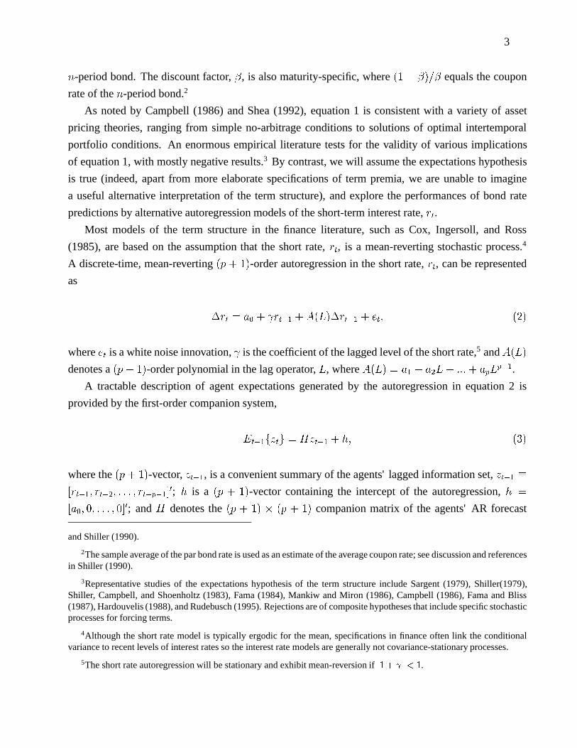
2.1 An Expectations Model of the Term Structure with Constant Endpoints

For coupon-bearing bonds, the linearized expectations model of the term structure is

Et�1frn;tg �= D�1n

n�1Xi=0

�iEt�1frt+ig+ bn; (1)

whereEt�1f:g denotes expectations based on information available at the end oft � 1; rn;t denotes

the nominal yield to maturity of then-period bond;rt is the one-month bond rate;Dn is the duration

associated with ann-period coupon bond;1 andbn is the constant term premium associated with the

1Dn � (1� �n)=(1� �), where� is the discount factor, see discussion in Shiller, Campbell, and Schoenholtz (1983)

3

n-period bond. The discount factor,�, is also maturity-specific, where(1 � �)=� equals the coupon

rate of then-period bond.2

As noted by Campbell (1986) and Shea (1992), equation 1 is consistent with a variety of asset

pricing theories, ranging from simple no-arbitrage conditions to solutions of optimal intertemporal

portfolio conditions. An enormous empirical literature tests for the validity of various implications

of equation 1, with mostly negative results.3 By contrast, we will assume the expectations hypothesis

is true (indeed, apart from more elaborate specifications of term premia, we are unable to imagine

a useful alternative interpretation of the term structure), and explore the performances of bond rate

predictions by alternative autoregression models of the short-term interest rate,rt.

Most models of the term structure in the finance literature, such as Cox, Ingersoll, and Ross

(1985), are based on the assumption that the short rate,rt, is a mean-reverting stochastic process.4

A discrete-time, mean-reverting(p + 1)-order autoregression in the short rate,rt, can be represented

as

�rt = a0 + rt�1 + A(L)�rt�1 + et; (2)

whereet is a white noise innovation, is the coefficient of the lagged level of the short rate,5 andA(L)

denotes a(p� 1)-order polynomial in the lag operator,L, whereA(L) = a1 + a2L+ ::: + apLp�1.

A tractable description of agent expectations generated by the autoregression in equation 2 is

provided by the first-order companion system,

Et�1fztg = Hzt�1 + h; (3)

where the(p+ 1)-vector,zt�1, is a convenient summary of the agents' lagged information set,zt�1 �

[rt�1; rt�2; : : : ; rt�p�1]0; h is a (p + 1)-vector containing the intercept of the autoregression,h =

[a0; 0; : : : ; 0]0; andH denotes the(p + 1) � (p + 1) companion matrix of the agents' AR forecast

and Shiller (1990).

2The sample average of the par bond rate is used as an estimate of the average coupon rate; see discussion and referencesin Shiller (1990).

3Representative studies of the expectations hypothesis of the term structure include Sargent (1979), Shiller(1979),Shiller, Campbell, and Shoenholtz (1983), Fama (1984), Mankiw and Miron (1986), Campbell (1986), Fama and Bliss(1987), Hardouvelis (1988), and Rudebusch (1995). Rejections are of composite hypotheses that include specific stochasticprocesses for forcing terms.

4Although the short rate model is typically ergodic for the mean, specifications in finance often link the conditionalvariance to recent levels of interest rates so the interest rate models are generally not covariance-stationary processes.

5The short rate autoregression will be stationary and exhibit mean-reversion ifj1 + j < 1.

4

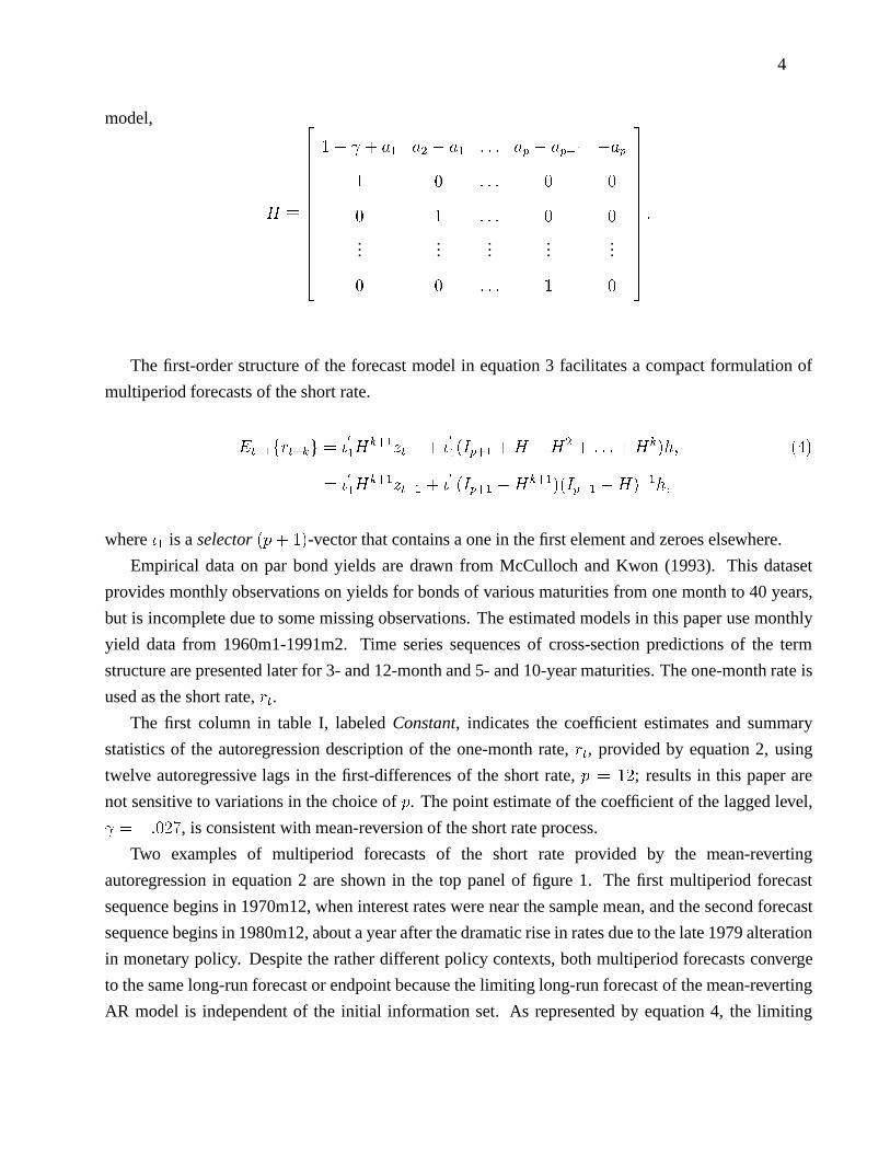
model,

H �

2666666666666664

1 + + a1 a2 � a1 : : : ap � ap�1 �ap

1 0 : : : 0 0

0 1 : : : 0 0

......

......

...

0 0 : : : 1 0

3777777777777775

:

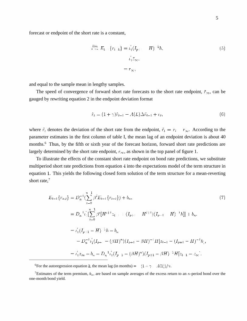
The first-order structure of the forecast model in equation 3 facilitates a compact formulation of

multiperiod forecasts of the short rate.

Et�1frt+kg = �0

1Hk+1zt�1 + �

0

1(Ip+1 +H +H2 + : : :+Hk)h; (4)

= �0

1Hk+1zt�1 + �

0

1(Ip+1 �Hk+1)(Ip+1 �H)�1h;

where�1 is aselector(p+ 1)-vector that contains a one in the first element and zeroes elsewhere.

Empirical data on par bond yields are drawn from McCulloch and Kwon (1993). This dataset

provides monthly observations on yields for bonds of various maturities from one month to 40 years,

but is incomplete due to some missing observations. The estimated models in this paper use monthly

yield data from 1960m1-1991m2. Time series sequences of cross-section predictions of the term

structure are presented later for 3- and 12-month and 5- and 10-year maturities. The one-month rate is

used as the short rate,rt.

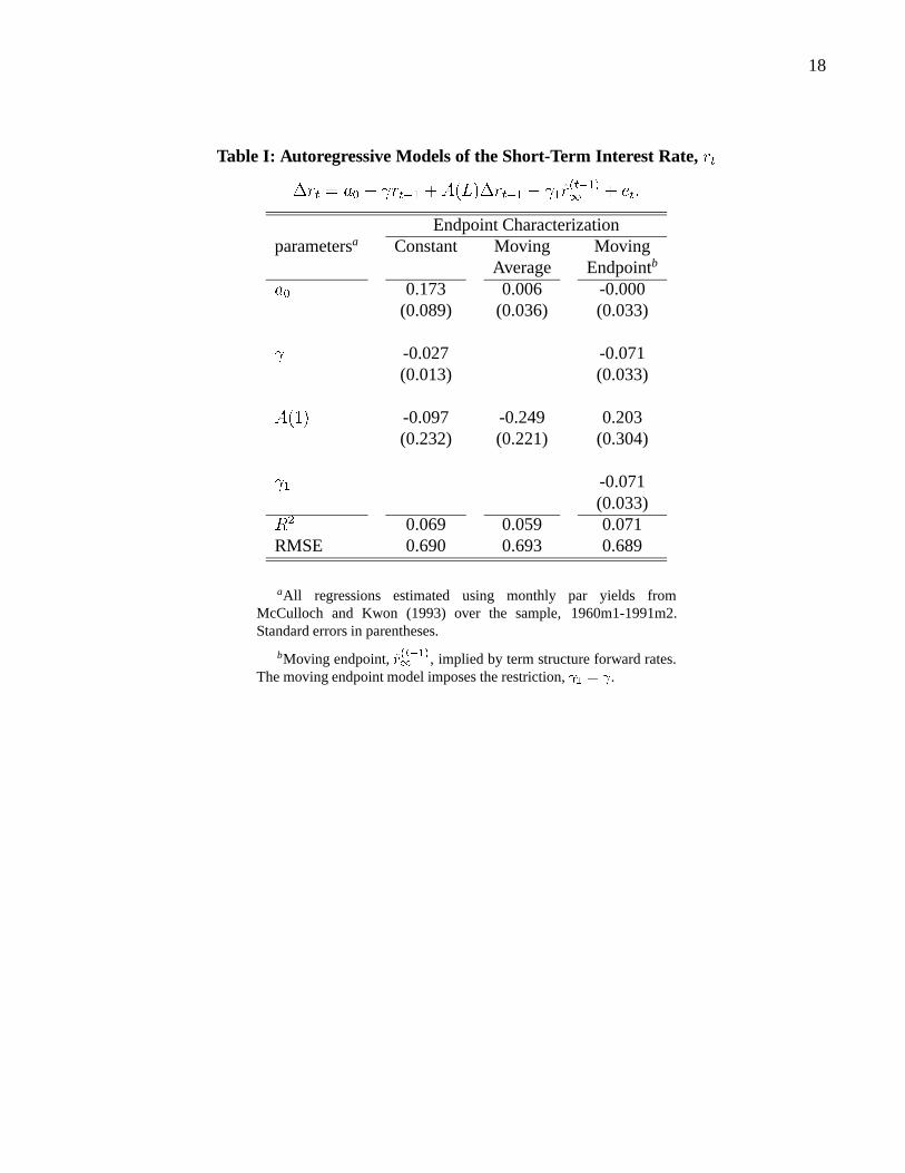
The first column in table I, labeledConstant, indicates the coefficient estimates and summary

statistics of the autoregression description of the one-month rate,rt, provided by equation 2, using

twelve autoregressive lags in the first-differences of the short rate,p = 12; results in this paper are

not sensitive to variations in the choice ofp. The point estimate of the coefficient of the lagged level,

= �:027, is consistent with mean-reversion of the short rate process.

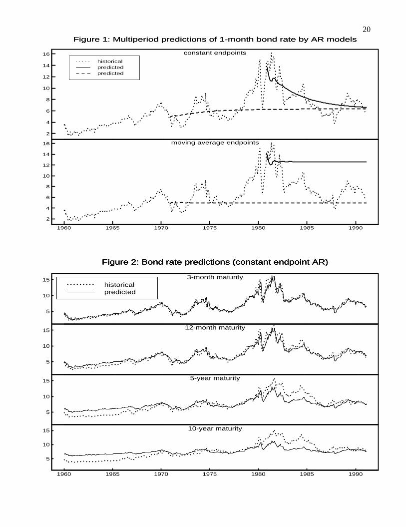
Two examples of multiperiod forecasts of the short rate provided by the mean-reverting

autoregression in equation 2 are shown in the top panel of figure 1. The first multiperiod forecast

sequence begins in 1970m12, when interest rates were near the sample mean, and the second forecast

sequence begins in 1980m12, about a year after the dramatic rise in rates due to the late 1979 alteration

in monetary policy. Despite the rather different policy contexts, both multiperiod forecasts converge

to the same long-run forecast or endpoint because the limiting long-run forecast of the mean-reverting

AR model is independent of the initial information set. As represented by equation 4, the limiting

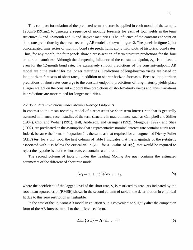
5

forecast or endpoint of the short rate is a constant,

limk!1 Et�1frt+kg = �

0

1(Ip+1 �H)�1h; (5)

= �0

1�z1;

= �r1;

and equal to the sample mean in lengthy samples.

The speed of convergence of forward short rate forecasts to the short rate endpoint,�r1, can be

gauged by rewriting equation 2 in the endpoint deviation format

~rt = (1 + )~rt�1 + A(L)�~rt�1 + et; (6)

where~rt denotes the deviation of the short rate from the endpoint,~rt = rt � �r1. According to the

parameter estimates in the first column of table I, the mean lag of an endpoint deviation is about 40

months.6 Thus, by the fifth or sixth year of the forecast horizon, forward short rate predictions are

largely determined by the short rate endpoint,�r1, as shown in the top panel of figure 1.

To illustrate the effects of the constant short rate endpoint on bond rate predictions, we substitute

multiperiod short rate predictions from equation4 into the expectations model of the term structure in

equation1. This yields the following closed form solution of the term structure for a mean-reverting

short rate,7

Et�1frn;tg = D�1n(n�1Xi=0

�iEt�1frt+ig) + bn; (7)

= D�1n�0

1[n�1Xi=0

�i[H i+1zt�1 + (Ip+1 �H i+1)(Ip+1 �H)�1h]] + bn;

= �0

1(Ip+1 �H)�1h+ bn

+D�1n�0

1(Ip+1 � (�H)n)(Ip+1 � �H)�1H[zt�1 � (Ip+1 �H)�1h];

= �0

1�z1 + bn +D�1n�0

1(Ip+1 � (�H)n)(Ip+1 � �H)�1H[zt�1 � �z1]:

6For the autoregression equation2, the mean lag (in months)= �(1 + �A(1))= .

7Estimates of the term premium,bn, are based on sample averages of the excess return to ann-period bond over theone-month bond yield.

6

This compact formulation of the predicted term structure is applied in each month of the sample,

1960m1-1991m2, to generate a sequence of monthly forecasts for each of four yields in the term

structure: 3- and 12-month and 5- and 10-year maturities. The influence of the constant endpoint on

bond rate predictions by the mean-reverting AR model is shown in figure 2. The panels in figure 2 plot

concatenated time series of monthly bond rate predictions, along with plots of historical bond rates.

Thus, for any month, the four panels show a cross-section of term structure predictions for the four

bond rate maturities. Although the dampening influence of the constant endpoint,�r1, is noticeable

even for the 12-month bond rate, the excessively smooth predictions of the constant-endpoint AR

model are quite evident for the longer maturities. Predictions of long-horizon yields are based on

long-horizon forecasts of short rates, in addition to shorter horizon forecasts. Because long-horizon

predictions of short rates converge to the constant endpoint, predictions of long-maturity yields place

a larger weight on the constant endpoint than predictions of short-maturity yields and, thus, variations

in predictions are more muted for longer maturities.

2.2 Bond Rate Predictions under Moving Average Endpoints

In contrast to the mean-reverting model of a representative short-term interest rate that is generally

assumed in finance, recent studies of the term structure in macrofinance, such as Campbell and Shiller

(1987), Choi and Wohar (1991), Hall, Anderson, and Granger (1992), Mougoue (1992), and Shea

(1992), are predicated on the assumption that a representative nominal interest rate contains a unit root.

Indeed, because the format of equation2 is the same as that required for an augmented Dickey-Fuller

(ADF) test for a unit root, the first column of table I indicates that the magnitude of thet-statistic

associated with is below the critical value (2:56 for a p-value of10%) that would be required to

reject the hypothesis that the short rate,rt, contains a unit root.

The second column of table I, under the headingMoving Average, contains the estimated

parameters of the differenced short rate model

�rt = a0 + A(L)�rt�1 + et; (8)

where the coefficient of the lagged level of the short rate, , is restricted to zero. As indicated by the

root mean squared error (RMSE) shown in the second column of table I, the deterioration in empirical

fit due to this zero restriction is negligible.

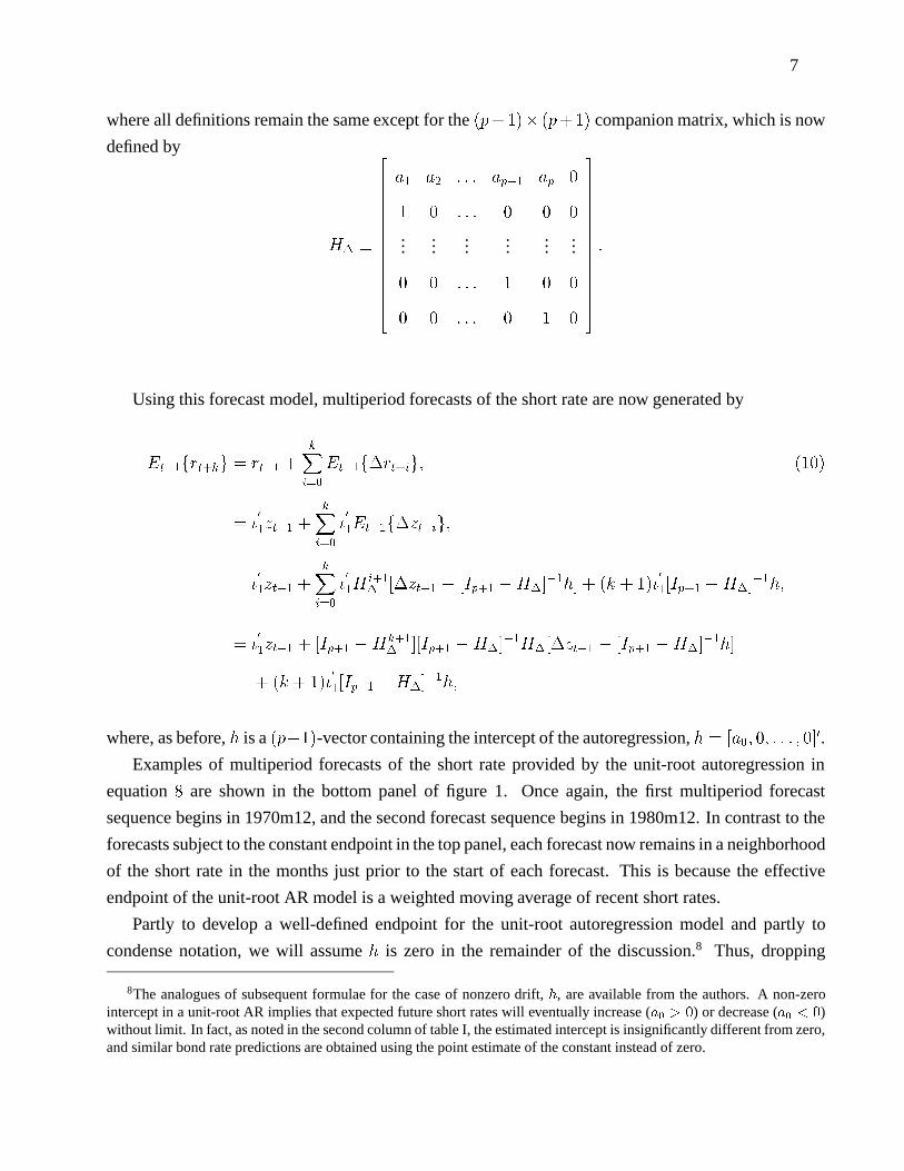
In the case of the unit-root AR model in equation8, it is convenient to slightly alter the companion

form of the AR forecast model to the differenced format

Et�1f�ztg = H��zt�1 + h; (9)

7

where all definitions remain the same except for the(p+1)� (p+1) companion matrix, which is now

defined by

H� �

2666666666666664

a1 a2 : : : ap�1 ap 0

1 0 : : : 0 0 0

......

......

......

0 0 : : : 1 0 0

0 0 : : : 0 1 0

3777777777777775

:

Using this forecast model, multiperiod forecasts of the short rate are now generated by

Et�1frt+kg = rt�1 +kX

i=0

Et�1f�rt+ig; (10)

= �0

1zt�1 +kX

i=0

�0

1Et�1f�zt+ig;

= �0

1zt�1 +kX

i=0

�0

1Hi+1� [�zt�1 � [Ip+1 �H�]

�1h] + (k + 1)�0

1[Ip+1 �H�]�1h;

= �0

1zt�1 + [Ip+1 �Hk+1� ][Ip+1 �H�]

�1H�[�zt�1 � [Ip+1 �H�]�1h]

+ (k + 1)�0

1[Ip+1 �H�]�1h;

where, as before,h is a(p+1)-vector containing the intercept of the autoregression,h = [a0; 0; : : : ; 0]0.

Examples of multiperiod forecasts of the short rate provided by the unit-root autoregression in

equation8 are shown in the bottom panel of figure 1. Once again, the first multiperiod forecast

sequence begins in 1970m12, and the second forecast sequence begins in 1980m12. In contrast to the

forecasts subject to the constant endpoint in the top panel, each forecast now remains in a neighborhood

of the short rate in the months just prior to the start of each forecast. This is because the effective

endpoint of the unit-root AR model is a weighted moving average of recent short rates.

Partly to develop a well-defined endpoint for the unit-root autoregression model and partly to

condense notation, we will assumeh is zero in the remainder of the discussion.8 Thus, dropping

8The analogues of subsequent formulae for the case of nonzero drift,h, are available from the authors. A non-zerointercept in a unit-root AR implies that expected future short rates will eventually increase (a0 > 0) or decrease (a0 < 0)without limit. In fact, as noted in the second column of table I, the estimated intercept is insignificantly different from zero,and similar bond rate predictions are obtained using the point estimate of the constant instead of zero.

8

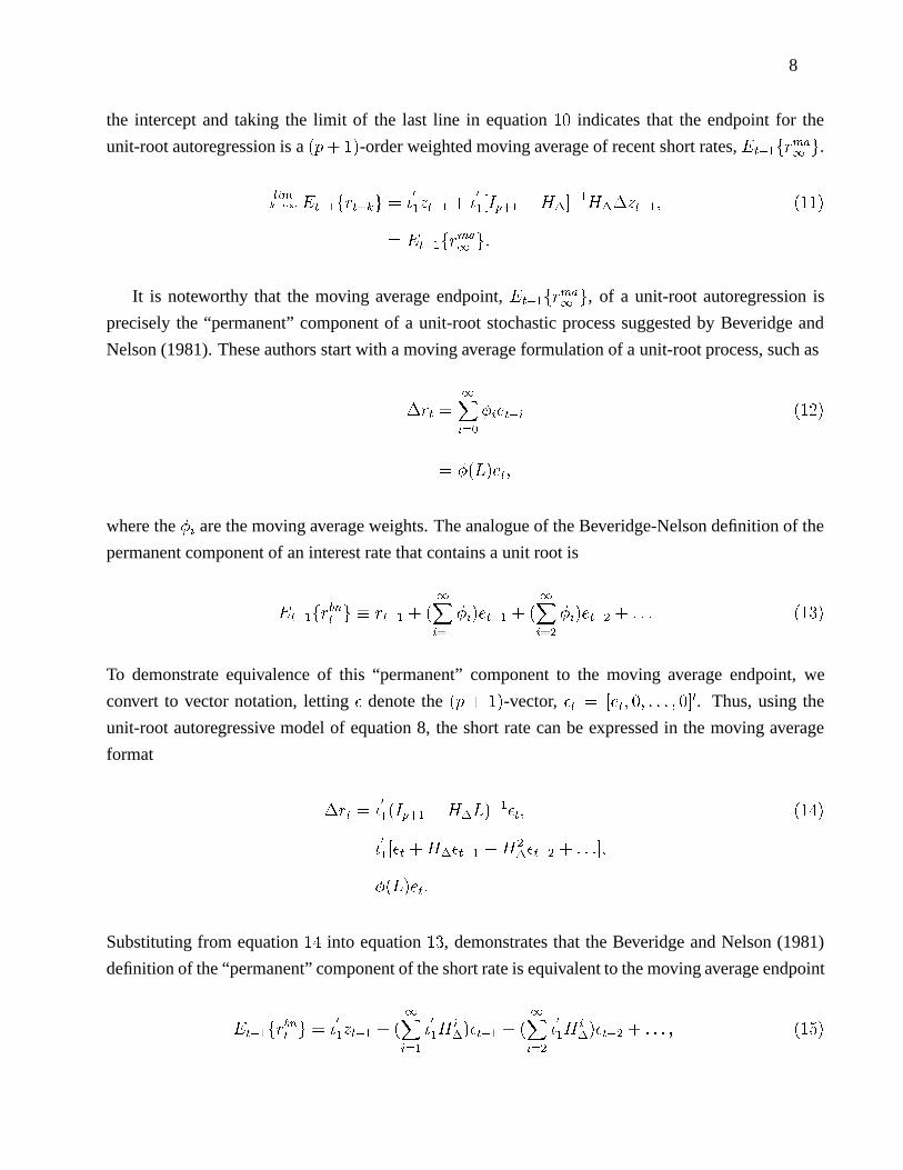
the intercept and taking the limit of the last line in equation10 indicates that the endpoint for the

unit-root autoregression is a(p+ 1)-order weighted moving average of recent short rates,Et�1frma

1g.

limk!1 Et�1frt+kg = �

0

1zt�1 + �0

1[Ip+1 �H�]�1H��zt�1; (11)

= Et�1frma

1g:

It is noteworthy that the moving average endpoint,Et�1frma

1g, of a unit-root autoregression is

precisely the “permanent” component of a unit-root stochastic process suggested by Beveridge and

Nelson (1981). These authors start with a moving average formulation of a unit-root process, such as

�rt =1Xi=0

�iet�i (12)

= �(L)et;

where the�i are the moving average weights. The analogue of the Beveridge-Nelson definition of the

permanent component of an interest rate that contains a unit root is

Et�1frbn

tg � rt�1 + (

1Xi=1

�i)et�1 + (1Xi=2

�i)et�2 + : : : (13)

To demonstrate equivalence of this “permanent” component to the moving average endpoint, we

convert to vector notation, letting� denote the(p + 1)-vector, �t = [et; 0; : : : ; 0]0. Thus, using the

unit-root autoregressive model of equation 8, the short rate can be expressed in the moving average

format

�rt = �0

1(Ip+1 �H�L)�1�t; (14)

= �0

1[�t +H��t�1 +H2��t�2 + : : :];

= �(L)et:

Substituting from equation14 into equation13, demonstrates that the Beveridge and Nelson (1981)

definition of the “permanent” component of the short rate is equivalent to the moving average endpoint

Et�1frbn

tg = �

0

1zt�1 + (1Xi=1

�0

1Hi

�)�t�1 + (1Xi=2

�0

1Hi

�)�t�2 + : : : ; (15)

9

= �0

1zt�1 + �0

1(Ip+1 �H�)�1[H��t�1 +H2

��t�2 + : : : ;

= �0

1zt�1 + �0

1(Ip+1 �H�)�1H��zt�1;

= Et�1frma

1g;

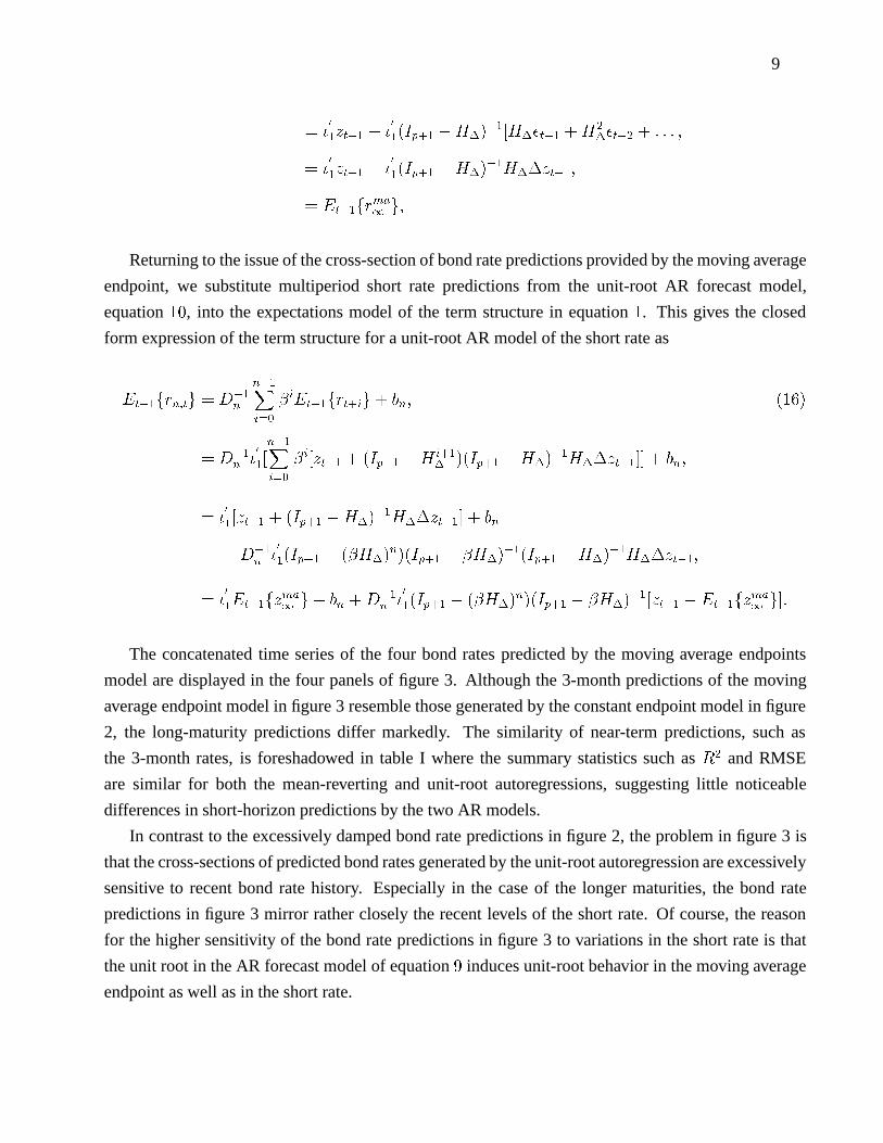
Returning to the issue of the cross-section of bond rate predictions provided by the moving average

endpoint, we substitute multiperiod short rate predictions from the unit-root AR forecast model,

equation10, into the expectations model of the term structure in equation1. This gives the closed

form expression of the term structure for a unit-root AR model of the short rate as

Et�1frn;tg = D�1n

n�1Xi=0

�iEt�1frt+ig+ bn; (16)

= D�1n�0

1[n�1Xi=0

�i[zt�1 + (Ip+1 �H i+1� )(Ip+1 �H�)

�1H��zt�1]] + bn;

= �0

1[zt�1 + (Ip+1 �H�)�1H��zt�1] + bn

�D�1n�0

1(Ip+1 � (�H�)n)(Ip+1 � �H�)

�1(Ip+1 �H�)�1H��zt�1;

= �0

1Et�1fzma

1g+ bn +D�1

n�0

1(Ip+1 � (�H�)n)(Ip+1 � �H�)

�1[zt�1 � Et�1fzma

1g]:

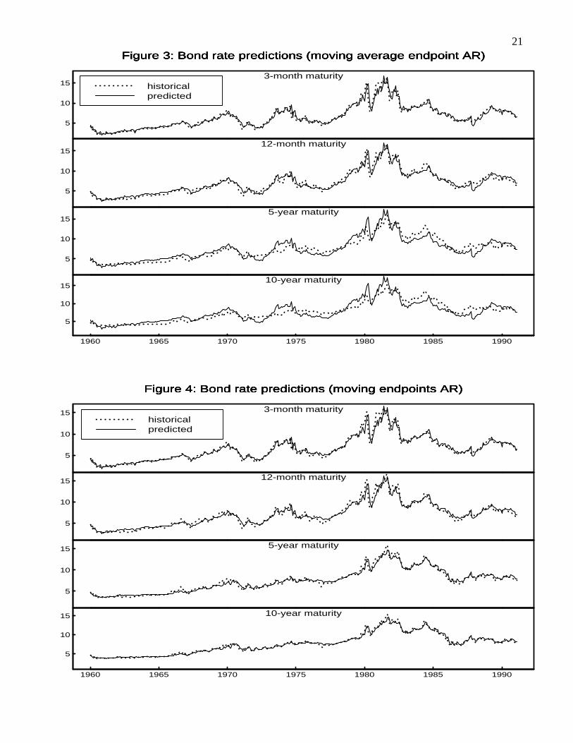
The concatenated time series of the four bond rates predicted by the moving average endpoints

model are displayed in the four panels of figure 3. Although the 3-month predictions of the moving

average endpoint model in figure 3 resemble those generated by the constant endpoint model in figure

2, the long-maturity predictions differ markedly. The similarity of near-term predictions, such as

the 3-month rates, is foreshadowed in table I where the summary statistics such asR2 and RMSE

are similar for both the mean-reverting and unit-root autoregressions, suggesting little noticeable

differences in short-horizon predictions by the two AR models.

In contrast to the excessively damped bond rate predictions in figure 2, the problem in figure 3 is

that the cross-sections of predicted bond rates generated by the unit-root autoregression are excessively

sensitive to recent bond rate history. Especially in the case of the longer maturities, the bond rate

predictions in figure 3 mirror rather closely the recent levels of the short rate. Of course, the reason

for the higher sensitivity of the bond rate predictions in figure 3 to variations in the short rate is that

the unit root in the AR forecast model of equation9 induces unit-root behavior in the moving average

endpoint as well as in the short rate.

10

3. Autoregressive Models with Moving Endpoints

Although it is evident from figure 2 that the interest rate endpoint is not fixed, it is equally apparent

from figure 3 that the unit-root description of nonstationarity in the interest rate endpoint is also

deficient. Unit-root stochastic processes are only one subset of the general class of nonstationary

time series, and it is well-known that standard tests for unit roots have low power against other

descriptions of nonstationarity, such as the episodic shifts analyzed in Perron (1989). There are ways

other than unit roots to characterize nonstationary movements. These include the shifting-regimes

models of Hamilton (1989), and detection of structural shifts or changepoints, such as Hinkley (1970)

and Andrews (1993).9

Rather than explore alternative statistical descriptions of nonstationary endpoints, this section

demonstrates that estimates of shifting perceptions by agents of endpoints can often be extracted from

observable information on the ex ante forecasts of agents. Two examples of ex ante estimates of

moving endpoints are discussed in this section. The first subsection indicates that implicit forward

rates in the term structure provide an effective measure of the interest rate endpoints embedded in

market multiperiod forecasts. The second subsection relates the moving endpoint of nominal interest

rates to the implied endpoint of expected inflation. Time series forecasts of these moving endpoint

models are compared with time series of a cross-section of historical bond rates in the term structure

and with time series of survey estimates of expected long-run inflation.

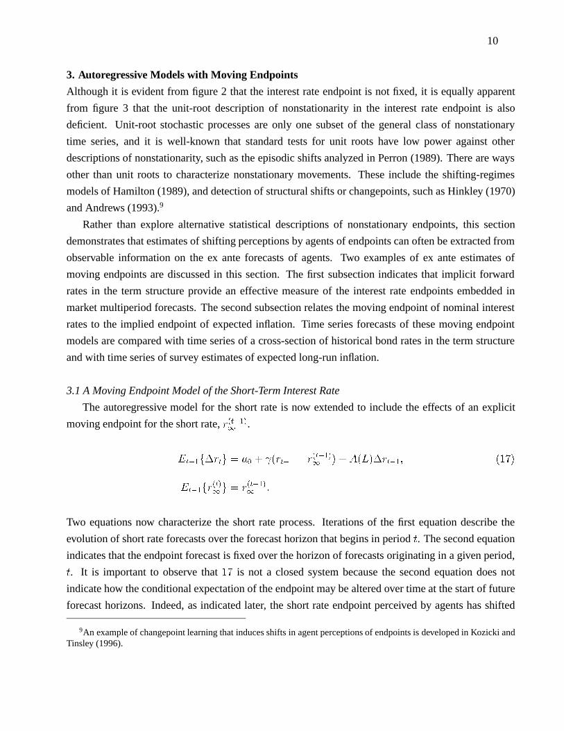
3.1 A Moving Endpoint Model of the Short-Term Interest Rate

The autoregressive model for the short rate is now extended to include the effects of an explicit

moving endpoint for the short rate,r(t�1)1

.

Et�1f�rtg = a0 + (rt�1 � r(t�1)1

) + A(L)�rt�1; (17)

Et�1fr(t)1g = r(t�1)

1:

Two equations now characterize the short rate process. Iterations of the first equation describe the

evolution of short rate forecasts over the forecast horizon that begins in periodt. The second equation

indicates that the endpoint forecast is fixed over the horizon of forecasts originating in a given period,

t. It is important to observe that17 is not a closed system because the second equation does not

indicate how the conditional expectation of the endpoint may be altered over time at the start of future

forecast horizons. Indeed, as indicated later, the short rate endpoint perceived by agents has shifted

9An example of changepoint learning that induces shifts in agent perceptions of endpoints is developed in Kozicki andTinsley (1996).

11

substantially over the historical sample.10

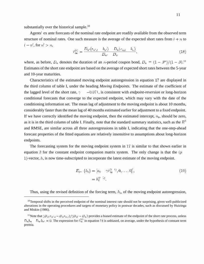
Agents' ex ante forecasts of the nominal rate endpoint are readily available from the observed term

structure of nominal rates. One such measure is the average of the expected short rates fromt + n to

t+ n0, for n0 > n,

r(t)1

=Dn0(rn0;t � bn0)�Dn(rn;t � bn)

Dn0 �Dn

; (18)

where, as before,Dn denotes the duration of ann-period coupon bond,Dn � (1 � �n)=(1 � �).11

Estimates of the short rate endpoint are based on the average of expected short rates between the 5-year

and 10-year maturities.

Characteristics of the estimated moving endpoint autoregression in equation17 are displayed in

the third column of table I, under the headingMoving Endpoints. The estimate of the coefficient of

the lagged level of the short rate, = �0:071, is consistent withendpoint-reversionor long-horizon

conditional forecasts that converge to the expected endpoint, which may vary with the date of the

conditioning information set. The mean lag of adjustment to the moving endpoint is about 10 months,

considerably faster than the mean lag of 40 months estimated earlier for adjustment to a fixed endpoint.

If we have correctly identified the moving endpoint, then the estimated intercept,a0, should be zero,

as it is in the third column of table I. Finally, note that the standard summary statistics, such as theR2

and RMSE, are similar across all three autoregressions in table I, indicating that the one-step-ahead

forecast properties of the fitted equations are relatively insensitive to assumptions about long-horizon

endpoints.

The forecasting system for the moving endpoint system in17 is similar to that shown earlier in

equation3 for the constant endpoint companion matrix system. The only change is that the(p +

1)-vector,h, is now time-subscripted to incorporate the latest estimate of the moving endpoint.

Et�1fhtg = [a0 � r(t�1)1

; 0; : : : ; 0]0

; (19)

= h(t�1)t :

Thus, using the revised definition of the forcing term,ht, of the moving endpoint autoregression,

10Temporal shifts in the perceived endpoint of the nominal interest rate should not be surprising, given well-publicizedalterations in the operating procedures and targets of monetary policy in postwar decades, such as discussed by Huizingaand Miskin (1986).

11Note that(Dn0rn0;t�Dnrn;t)=(Dn0 �Dn) provides a biased estimate of the endpoint of the short rate process, unless

Dnbn�Dn0bn0 = 0. The expression forr(t)1

in equation18 is unbiased, on average, under the hypothesis of constant termpremia.

12

multiperiod forecasts of the short rate are now provided by

Et�1frt+kg = �0

1(Ip+1 �H)�1h(t�1)t + �

0

1Hk+1[zt�1 � (Ip+1 �H)�1h

(t�1)t ]; (20)

= �0

1z(t�1)1

+ �0

1Hk+1[zt�1 � z(t�1)

1];

where the effective moving endpoint will be equivalent to the measured short rate endpoint,�0

1z(t�1)1

=

r(t�1)1

if the estimated intercept is zero,a0 = 0.

Finally, the closed form solutions for term structure predictions under the moving endpoint

autoregression are obtained by substituting the bond rate predictions from equation20 into equation1,

giving

Et�1rn;t = D�1n�0

1(n�1Xi=0

�iEt�1frt+ig) + bn; (21)

= �0

1z(t�1)1

+ bn +D�1n�0

1(Ip+1 � (�H)n)(Ip+1 � �H)�1H[zt�1 � z(t�1)1

]:

The panels of figure 4 display the concatenated time series of the cross-section of four bond rates

predicted by the moving endpoint autoregression. Unlike the term structure predictions of the constant

and moving average endpoint models in figures 2 and 3, the bond rate predictions of the moving

endpoints model closely track the historical bond rates at each of the selected four maturities in the

term structure. Since each maturity rate in the predicted term structure cross-section is generated by the

same autoregression model, the moving endpoints model generally supports the internal consistency

of agent ex ante forecasts contained in the historical term structure.

In principle, the moving endpoint model should be expected to dominate the other two endpoint

specifications because it is less restrictive in use of available information. The structural bond yield

model with the moving short rate endpoint,r(t�1)1

, can be interpreted as a two-factor model of the

term structure of interest rates where one factor is identified as the endpointr(t�1)1

and the second

factor is identified as the deviation of the short rate from that endpoint. By contrast, the constant and

moving average endpoint autoregressions are one-factor models where the short rate is identified as

the single factor. Because the performance of two-factor models should be expected to dominate that

of one-factor models, yield predictions generated by the model using the moving short rate endpoint,

r(t�1)1

, should generally outperform yield predictions based on constant or moving average endpoint

characterizations.12

12Subsequent work will indicate that standard literature suggestions to increase the dimension of the information set ofagents, such as the addition of a spread between a long and short rate to the short rate equation, are unlikely to approximate

13

3.2 Alternative Forecast Models of Expected Inflation

Another relationship that is based on an assumed internal consistency in the ex ante forecasts of agents

is the standard Fisherian decomposition of a nominal interest rate into the expected real rate and

expected inflation. In the current context, the after-tax nominal rate endpoint can be partitioned into

an expected real rate endpoint and an expected inflation endpoint.

(1� �)r(t)1

= �(t)1

+ �(t)1; (22)

where� denotes the marginal tax rate on bond earnings, and�(t)1

is the t-period estimate of the after-tax

real rate endpoint. Thus, equation22 suggests that a transformation of the nominal rate endpoint,

such as that used in the preceding section, might provide an internally consistent estimate of agents'

evolving perception of expected long-run inflation,�(t)1

.

The procedure used here to extract the implicit ex ante inflation endpoint from the nominal rate

endpoint rests on two additional approximations. First is the assumption that the after-tax real rate

endpoint is a constant. This is tantamount to the assumption that the after-tax real interest rate is

mean-reverting. Mean-reverting behavior, or even constancy, of the real rate is not an uncommon

specification in finance, Fama (1975); theoretical reasons and empirical evidence for this assumption,

absent marked shifts in fiscal policy not captured by changes in the tax rate,� , are discussed in

Kozicki and Tinsley (1996). Consequently, we will assume the constant after-tax real rate endpoint is

a maintained hypothesis.

A more nonstandard assumption in analyses of real rate arbitrage is the use of a nonzero marginal

tax rate. However, studies by McCulloch (1975) and Crowder and Hoffman (1996) suggest that the tax

rate on Treasury earnings falls in the interval,:20 � � � :30. Using flow of funds estimates of sectoral

holdings of Treasury securities, we estimate that the effective tax rate on earnings of US Treasuries,

averaged over the 1960-90 sample, is about thirty percent,� = 0:30.

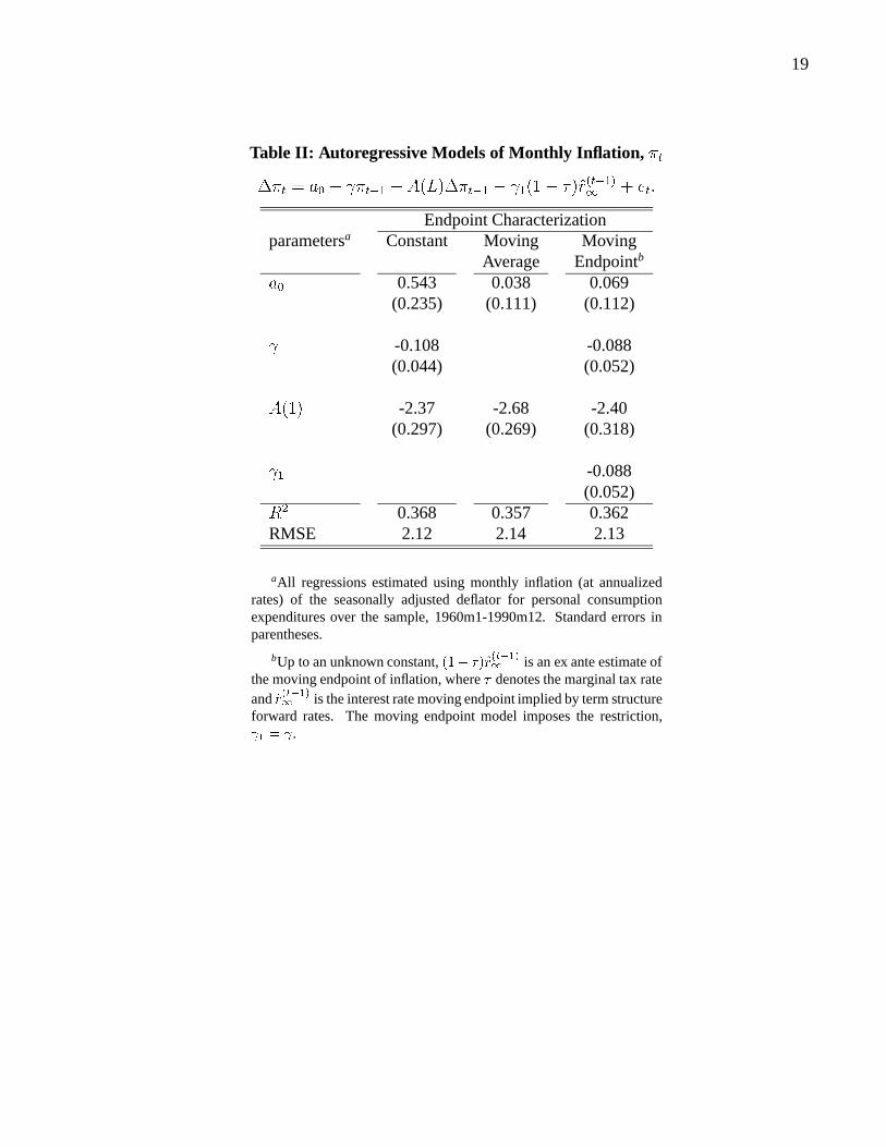
Analogous to the alternative models estimated for the monthly interest rate, three endpoint

autoregression models are estimated for monthly inflation,�t. Monthly inflation of the deflator for

personal consumption expenditures is expressed at annual rates. The formats of the regressions are

identical to those used for the monthly interest rate, except for a smaller number of autoregressive

lags,p = 6, and a sample span of 1960m1-1990m12.

The estimated parameters and summary statistics of theconstantendpoint, moving average

endpoint, andmoving endpointAR models of inflation are listed, respectively, in the three columns of

table II. As with the interest rate examples, there is little to choose among the equations on the basis of

the behavior of a two-factor moving endpoint model.

14

conventional summary statistics such as theR2 and RMSE. Adjustment of inflation predictions to the

inflation endpoints are sluggish for both the models with constant and moving endpoints, with a mean

lag of about 30 months for the former and 38 months for the latter. Although the estimated intercept is

not significantly different from zero in the moving endpoint autoregression, the point estimate suggests

an after-tax annual real rate endpoint for 1-month US Treasuries of about 80 basis points,�1 � �a0= .

In contrast to the term structure, available measurements of agent multiperiod predictions of

inflation are more limited. Several surveys of expected inflation in the United States are available but

most focus on short-term expectations of inflation. For the purpose of drawing comparisons among

the three inflation forecast models, this is a serious drawback since we know from the results for

multiperiod interest rate forecasts that short-horizon forecasts will be similar for all three models.

Two notable exceptions are a survey of market participants conducted in the 1980s by Richard

Hoey, an economist at Drexel Burnham Lambert, which asked for 10-year inflation forecasts and a

survey of household estimates of inflation in the next 5-10 years, conducted by the Michigan Survey

Research Center. Although the Hoey survey has been discontinued, a contiguous quarterly series of

expected 10-year inflation is assembled for the span, 1980q4-1990q4. Similarly, although there are

many missing observations for the Michigan survey, a quarterly series of long-term expected inflation

for the span, 1982q3-1990q4. is assembled by using the “last known estimate” to fill in missing

observations.

Predictions of 10-year inflation rates are generated by the equations used to generate 10-year bond

rates, with adjustments for undiscounted averages. In other words, similar to alterations required

for zero-coupon bonds, the closed-form solutions for the coupon-bond term structure in equations

7, 10, and16 are adjusted for 10-year averaging by setting the discount factor to unity,� = 1:0,

and the duration to 120 months,Dn = 120. The three endpoint autogression forecast models are

used to generate concatenated time series of monthly predictions of 10-year inflation rates. These

are averaged to quarterly observations, to match the frequency of the assembled survey estimates of

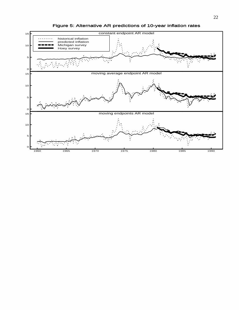
expected long-term inflation, and plotted in the three panels of figure 5.

In somewhat of a replay of the properties of the bond rate predictions, the first panel of figure

5 indicates that the 10-year inflation rates predicted by the constant endpoint model are too smooth

relative to the survey estimates. Likewise, the 10-year inflation rates predicted by the moving average

autoregression, shown in the second panel of figure 5, more closely track the path of historical inflation

than the survey estimates.

By contrast, the third panel of figure 5 indicates that the predictions of 10-year inflation rates

generated by the moving endpoint model of inflation move quite closely with the available observations

on survey estimates of expected inflation, slightly favoring the Michigan survey estimate over the Hoey

survey estimate in the last few years of the sample. Since none of the information in either of the two

surveys was used to estimate the moving endpoint model of inflation, this is a very remarkable result.

15

Also, the fact that this relatively close correspondence is generated by a moving endpoints model based

on a linear transformation of the endpoint in the term structure suggests that the ex ante forecasts of

inflation that are plausibly embedded in bond rates are internally consistent with the ex ante forecasts

of long-term inflation measured by the surveys.

4. Concluding Comments

Results in this paper suggest that more flexible specifications of boundary values or transversality

conditions are required, along with estimation of Euler equation descriptions of dynamic adjustments,

if empirical models in macroeconomics and finance are to be successful in rational interpretations of

agent behavior. In particular, the two alternatives of constant or moving average long-run boundary

values that are implied by standard time series models are shown to be inconsistent with the implicit

endpoints of agents' ex ante forecasts.

The examples used in this paper to illustrate the strong effects of terminal boundary conditions on

multiperiod forecasts are simple autoregression implementations of expectations models of the term

structure and expected inflation. These examples are useful because measurements of agent forecasts

of forward interest rates and expected inflation are available for comparison with model predictions.

Also, assuming auction markets are efficient at least at monthly frequencies, measured outcomes are

unlikely to be significantly distorted by transaction costs or other inhibiting frictions on agent behavior.

Neither mean-reverting autoregressions, with constant endpoints, nor unit-root autoregressions,

with moving average endpoints, are able to adequately track the historical movements of a

cross-section of bond rates in the term structure or variations in survey estimates of long-term inflation.

In contrast, the predictions by interest rate and inflation autoregressions with moving endpoints are able

to reproduce historical shifts in both the term structure and survey measures of expected inflation. The

implicit endpoint estimates used in this paper, inferred from the far end of the term structure, vary

considerably over time but not in a way that is consistent with unit root specifications.

Implicit endpoints, extracted from observable agent forecasts, are useful in testing the internal

consistency of market ex ante forecasts, such as the demonstration that the same moving endpoint

model of the short rate can capture time variations in the cross-section of bond rates in the term

structure, and that a Fisherian decomposition of bond rates into an after-tax real rate and expected

inflation appears to be broadly consistent with survey estimates of long-term inflation. The alternative

estimates of expected inflation by conventional time series models would deliver very different

estimates of ex ante real interest rates to monetary policy advisors, with potentially erroneous estimates

of agents' perceptions of current and expected policy.

Moving endpoints are consistent with learning by agents of unpredictable changes in steady-state

or long-run outcomes, such as alterations in government long-run policies or permanent changes in

the aspirations or behaviors of other market participants. Unlike the gradual outcomes of Kalman

16

filtering modeling, expanding-sample regressions, or other forms of incremental learning by linear

projections, the implicit endpoints used here seem to indicate that endpoint learning may be nonlinear,

with intervals of small changes followed abruptly by large shifts in beliefs. Developing endogenous

models of agents' perceptions of long-run endpoints is a challenging task for future work.13

References

Andrews, D., “Tests for Parameter Instability and Structural Change with Unknown Change Point,”Econometrica, 61, 4, July 1993, 821-56.

Beveridge, S. and C. Nelson, “A New Approach to Decomposition of Economic Time Seriesinto Permanent and Transitory Components with Particular Attention to Measurement of the' Business Cycle' ,”Journal of Monetary Economics, 7, 2, March 1981, 151-74.

Campbell, J., “A Defense of Traditional Hypotheses about the Term Structure of Interest Rates,”Journal of Finance, 41, 1986, 183-93.

Campbell, J. and R. Shiller, “Cointegration and Tests of Present Value Models,”Journal of PoliticalEconomy, 95, 5, 1987, 1062-88.

Choi, S., and M. Wohar, “New Evidence Concerning the Expectations Theory for the Short End ofthe Maturity Spectrum,”The Journal of Financial Research, 14, 1991, 83-92.

Cox, J., J. Ingersoll, and S. Ross, “A Theory of the Term Structure of Interest Rates,”Econometrica,53, 2, March 1985, 385-407.

Crowder, W. and D. Hoffman, “The Long Run Relationship Between Nominal Interest Ratesand Inflation: The Fisher Equation Revisited,”Journal of Money, Credit, and Banking, 28,1, February 1996, 102-18.

Fama, E., “Short-Term Interest Rates as Predictors of Inflation,”American Economic Review, 65,3,June 1975, 269-82.

Fama, E., “The Information in the Term Structure,”Journal of Financial Economics, 13, 1984,509-28.

Fama, E. and R. Bliss, “The Information in Long-Maturity Forward Rates,”The AmericanEconomic Review, 77, 1987, 680-92.

Hall, A., H. Anderson, and C. Granger, “A Cointegration Analysis of Treasury Bill Yields,”TheReview of Economics and Statistics, 74, 1, February 1992, 116-26.

Hamilton, J., “A New Approach to the Economic Analysis of Nonstationary Time Series and theBusiness Cycle,”Econometrica, 57, 1989, 357-84.

Hardouvelis, G., “The Predictive Power of the Term Structure During Recent Monetary Regimes,”Journal of Finance, 43, 1988, 339-56.

Hinkley, D., “Inference About the Change-Point in a Sequence of Random Variables,”Biometrika,57, 1, April 1970, 1-17.

13An example of changepoint learning by agents of perceived shifts in the inflation target of monetary policy is discussedin Kozicki and Tinsley (1996).

17

Huizinga, J. and F. Mishkin, “Monetary Policy Regime Shifts and the Unusual Behavior of RealInterest Rates,” in K. Brunner and A. Meltzer (eds.),Carnegie-Rochester Conference Series onPublic Policy, 24, 1986, 231-74.

Kozicki, S. and P. Tinsley, “Moving Endpoints in the Term Structure of Interest Rates,”FRBKC/FRB staff working paper, May 1996.

Mankiw, G., and J. Miron, “The Changing Behavior of the Term Structure of Interest Rates,”Quarterly Journal of Economics, 101, 1986, 211-28.

McCulloch, H., “The Tax-Adjusted Yield Curve,”The Journal of Finance, 30, 1975, 811-30.

McCulloch, H. and H. Kwon, “U.S. Term Structure Data, 1947-1991,” Ohio State UniversityWorking Paper 93-6, March 1993.

Mougoue, M., “The Term Structure of Interest Rates as a Cointegrated System: Empirical Evidencefrom the Eurocurrency Market,”The Journal of Financial Research, 15, 3, 1992, 285-96.

Perron, P., “The Great Crash, the Oil Price Shock, and the Unit Root Hypothesis,”Econometrica,57, 1989, 1361-401.

Rudebusch, G., “Federal Reserve Interest Rate Targeting, Rational Expectations, and the TermStructure,”Journal of Monetary Economics, 35, 1995, 245-74.

Sargent, T., “A Note on Maximum Likelihood Estimation of the Rational Expectations Model ofthe Term Structure,”Journal of Monetary Economics, 5, 1979, 133-43.

Shea, G., “Benchmarking the Expectations Hypothesis of the Interest-Rate Term Structure: AnAnalysis of Cointegration Vectors,”Journal of Business and Economic Statistics, 10, 3, July1992, 347-66.

Shiller, R., “The Volatility of Long-Term Interest Rates and Expectations Models of the TermStructure,”Journal of Political Economy, 67, 6, December 1979, 190-219.

Shiller, R., “The Term Structure of Interest Rates,” in B. Friedman and F. Hahn (eds.)Handbookof Monetary Economics, vol. I, 1990, 627-722.

Shiller, R., J. Campbell, and K. Schoenholtz, “Forward Rates and Future Policy: Interpreting theTerm Structure of Interest Rates,”Brookings Papers, 1983, 173-223.

18

Table I: Autoregressive Models of the Short-Term Interest Rate,rt

�rt = a0 + rt�1 + A(L)�rt�1 � 1r(t�1)1

+ et:

Endpoint Characterizationparametersa Constant Moving Moving

Average Endpointb

a0 0.173 0.006 -0.000(0.089) (0.036) (0.033)

-0.027 -0.071(0.013) (0.033)

A(1) -0.097 -0.249 0.203(0.232) (0.221) (0.304)

1 -0.071(0.033)

R2 0.069 0.059 0.071RMSE 0.690 0.693 0.689

aAll regressions estimated using monthly par yields fromMcCulloch and Kwon (1993) over the sample, 1960m1-1991m2.Standard errors in parentheses.

bMoving endpoint,r(t�1)1

, implied by term structure forward rates.The moving endpoint model imposes the restriction, 1 = .

19

Table II: Autoregressive Models of Monthly Inflation, �t

��t = a0 + �t�1 + A(L)��t�1 � 1(1� �)r(t�1)1

+ et:

Endpoint Characterizationparametersa Constant Moving Moving

Average Endpointb

a0 0.543 0.038 0.069(0.235) (0.111) (0.112)

-0.108 -0.088(0.044) (0.052)

A(1) -2.37 -2.68 -2.40(0.297) (0.269) (0.318)

1 -0.088(0.052)

R2 0.368 0.357 0.362RMSE 2.12 2.14 2.13

aAll regressions estimated using monthly inflation (at annualizedrates) of the seasonally adjusted deflator for personal consumptionexpenditures over the sample, 1960m1-1990m12. Standard errors inparentheses.

bUp to an unknown constant,(1� �)r(t�1)1

is an ex ante estimate ofthe moving endpoint of inflation, where� denotes the marginal tax rateandr(t�1)

1is the interest rate moving endpoint implied by term structure

forward rates. The moving endpoint model imposes the restriction, 1 = .

20

2

4

6

8

10

12

14

16

Figure 1: Multiperiod predictions of 1-month bond rate by AR models

historicalpredictedpredicted

constant endpoints

2

4

6

8

10

12

14

16

1960 1965 1970 1975 1980 1985 1990

Figure 1: Multiperiod predictions of 1-month bond rate by AR models

moving average endpoints

5

10

15

Figure 2: Bond rate predictions (constant endpoint AR)

historicalpredicted

3-month maturity

5

10

15


12-month maturity

5

10

15


5-year maturity

5

10

15

1960 1965 1970 1975 1980 1985 1990


10-year maturity

21

5

10

15

Figure 3: Bond rate predictions (moving average endpoint AR)

historicalpredicted

3-month maturity

5

10

15


12-month maturity

5

10

15


5-year maturity

5

10

15

1960 1965 1970 1975 1980 1985 1990


10-year maturity

5

10

15

Figure 4: Bond rate predictions (moving endpoints AR)

historicalpredicted

3-month maturity

5

10

15


12-month maturity

5

10

15


5-year maturity

5

10

15

1960 1965 1970 1975 1980 1985 1990


10-year maturity

22

0

5

10

15

Figure 5: Alternative AR predictions of 10-year inflation rates

historical inflationpredicted inflationMichigan surveyHoey survey

constant endpoint AR model

0

5

10

15


moving average endpoint AR model

0

5

10

15

1960 1965 1970 1975 1980 1985 1990


moving endpoints AR model

MOVING ENDPOINTS AND THE INTERNAL CONSISTENCY … · MOVING ENDPOINTS AND THE INTERNAL CONSISTENCY...

Documents

Transcript of MOVING ENDPOINTS AND THE INTERNAL CONSISTENCY … · MOVING ENDPOINTS AND THE INTERNAL CONSISTENCY...