MOTION VECTOR FIELD ESTIMATION USING … · MOTION VECTOR FIELD ESTIMATION USING BRIGHTNESS...

MOTION VECTOR FIELD ESTIMATION USING BRIGHTNESS CONSTANCYASSUMPTION AND EPIPOLAR GEOMETRY CONSTRAINT

S. Hosseinyalamdarya, , A. Yilmaza,

a Photogrammetric Computer Vision, Civil Engineering Department, The Ohio State University (hosseinyalamdary.1, yilmaz.15)@osu.edu

Commission VI, WG VI/4

KEY WORDS: IMU, Camera-IMU Integration, Visual-Inertial, Epipolar Geometry Constraint, Brightness Constancy Assumption,Optical Flow

ABSTRACT:

In most Photogrammetry and computer vision tasks, finding the corresponding points among images is required. Among many, theLucas-Kanade optical flow estimation has been employed for tracking interest points as well as motion vector field estimation. Thispaper uses the IMU measurements to reconstruct the epipolar geometry and it integrates the epipolar geometry constraint with thebrightness constancy assumption in the Lucas-Kanade method. The proposed method has been tested using the KITTI dataset. Theresults show the improvement in motion vector field estimation in comparison to the Lucas-Kanade optical flow estimation. The sameapproach has been used in the KLT tracker and it has been shown that using epipolar geometry constraint can improve the KLT tracker.It is recommended that the epipolar geometry constraint is used in advanced variational optical flow estimation methods.

1. INTRODUCTION

Without the loss of generality, the motion vector field computedby most optical flow estimation methods provides dense pixelcorrespondences between consecutive images, which is requiredin applications such as 3D recovery, activity analysis, image-based rendering and modeling (Szeliski, n.d.). It is also a pre-processing step for the higher level missions like scene under-standing. Despite its common applicability, precise optical flowestimation remains an unresolved problem in computer vision.While advances have been made, unaccounted variations in thescene content and depth discontinuities pose challenges to opti-cal flow estimation.

Optical flow was introduced in the 1980s, and is based on thebrightness constancy assumption between matching pixels in con-secutive images. However, the brightness constancy does not pro-vide adequate constraint to estimate the flow vector and spatialsmoothness constraint has been utilized by Lucas and Kanade(Lucas and Kanade, 1981) and Horn and Schunck (Horn andSchunck, 1981) to overcome this limitation. The spatial smooth-ness constraint, however, blurs the object boundaries in the es-timation motion vector field. Researchers have attempted to ad-dress this shortcoming by extending the Horn and Schuck’s ap-proach. Brox et al. (Brox et al., 2004) introduced a gradientconstancy term, a spatio-temporal smoothness term in the costfunction that was in the form of L1 norm. In a follow up study,the authors employed a descriptor matching strategy to estimatethe optical flow in the case of large displacements (Brox and Ma-lik, 2011). While improves the results, such temporal smoothnessheuristics do not truly reflect the changes in the optical flow ap-propriately. Total variation has been employed to estimate theoptical flow estimation (Zach et al., 2007, Javier Sanchez1 et al.,2013).

Due to the complex camera and object motions, modeling tempo-ral changes in optical flow using only the image information is adifficult task. In contrast to extensive studies on image based esti-mation of the optical flow, few studies has been conducted on us-ing other complimentary sensors to improve the results. Hwangboet al. 2008 have used homography transformation based on the

rotation measurements collected by gyroscope and approximatedthe neighborhood of the corresponding pixels. They showed thatthe KLT tracker initialized by rotational homography works bet-ter in handling the fast motion and rotation. Wedel et al. (Wedeland Cremers, 2011) have combined the epipolar geometry andoptical flow to estimate the position, velocity and orientation ofthe moving objects in the scene. IMU measurements has beenemployed to cancel out the camera motion and recover the pureobject motion. Slesareva et al. (Slesareva et al., 2005) used theepipolar geometry constraint as a hard constraint and Valgaerts etal. (Valgaerts et al., 2008) has minimized the epipolar geometryconstraint associated with the brightness constancy assumption.

In another study, the sensed gravity in IMU has been used asthe vertical reference to find the horizon line and vertical van-ishing point in the images (Corke et al., 2007). The integrationof the IMU measurements and the estimated pose using imagesequences has been extensively studied (Jones and Soatto, 2010,Kelly and Sukhatme, 2011, Li and Mourikis, 2013). Leung andMedioni (Leung and Medioni, 2014) have used the IMU mea-surements to detect the ground plane and use the points on theground plane to estimation the pose of the camera. The IMUmeasurements has been used to compensate the camera motionblur (Joshi et al., 2010).

In this paper, the motion vector field is estimated using epipolargeometry constraint. The epipolar geometry based on the IMUmeasurements are used to formulate the optical flow betweenconsecutive images with respect to both rotation and translationof the camera. The KITTI dataset is employed to evaluate theproposed method and the results are compared to a brightnessconstancy based the Lucas-Kanade optical flow estimation. Theresults show significant improvement in optical flow estimationusing the proposed approach.

In the next section, the brightness constancy based optical flowestimation and the epipolar geometry is briefly explained. An ap-proach has been proposed in section 3 which solve the motionvector field using brightness constancy and epipolar geometry.Section 4 explains evaluation of the proposed approach and pro-vide the results for the KITTI dataset. In final section, it is drawn

ISPRS Annals of the Photogrammetry, Remote Sensing and Spatial Information Sciences, Volume II-1, 2014ISPRS Technical Commission I Symposium, 17 – 20 November 2014, Denver, Colorado, USA

This contribution has been peer-reviewed. The double-blind peer-review was conducted on the basis of the full paper.doi:10.5194/isprsannals-II-1-9-2014 9

conclusion for this paper.

2. BACKGROUND

In spite of great improvements in optical flow estimation over thelast two decades, exploiting complimentary sensory data for op-tical flow estimation has not extensively been studied. Hence, inorder to facilitate the proposed discussion we first introduce somebasic concepts of optical flow and IMU measurements, whichwill be followed by a discussion on how the fusion of the twosensory data works to aid optical flow estimation.

2.1 brightness constancy assumption

Optical flow estimation is based on the brightness (or color) con-stancy assumption. It means that two corresponding pixels inconsecutive images at times t and t + 1 should have the samebrightness:

I(x, y, t) = I(x+ u, y + v, t+ 1). (1)

where x, y = pixel coordinatesu, v = motion vectorI(x, y, t) = brightness of the pixel which is anon linear function of pixel coordinates and time

Equation (1) expresses a non-linear functional which can be lin-earized using Taylor series expansion

Ixu+ Iyv + It = 0. (2)

where Ix = ∂I(x+u,y+v,t+1)∂x

Iy = ∂I(x+u,y+v,t+1)∂y

It = ∂I(x+u,y+v,t+1)∂t

The brightness constancy, however, provides a single constraintfor estimation of motion vector which has two unknowns. A typi-cal constraint used many is to assume that the neighboring pixelsshare the same motion, such that an overdetermined system ofequations can estimate the motion parameters. This effectivenesscomes at the expense of blurring the object and depth boundariesand creates incorrect results. Assuming that the neighboring pix-els move together, the motion vector can be estimated

l = Au. (3)

where A =

Ix(1) Iy(1)Ix(2) Iy(2)

......

Ix(N) Iy(N)

u =

[uv

]

l =

It(1)It(2)

...It(N)

the numbers in parenthesis is the number of eachpixel in a neighborhood

Equation (3) can be estimated using least squares

u = (N)−1c. (4)

where N = AT Ac = AT l

The covariance matrix of the estimation motion vector field is

Σu = σ20N−1 (5)

where σ20 = reference variance

Σu = the covariance matrix of the estimatedmotion vector field

The Lucas-Kanade optical flow can be improved if a filter is usedin the neighborhood. First, the gaussian filter which the centralpixel of the neighborhood has more contribution in the opticalflow estimation improves the motion vector field estimation. Sec-ond, the anisotropic filter which suppresses the contribution of thepixels with different brightness values and therefore, the similarpixels have more impact on the motion vector field estimation.The bilateral filter, which has been used in this paper, combinesthe gaussian filer and anisotropic filter

w(i, j, k, l) = e(− (i−k)2+(j−l)2

2σ2d

)− ||I(i,j)−I(k,l)||2σ2r

)

. (6)

where i, j = coordinates of the central pixel in theneghborhoodj, k = coordinates of the each pixel in theneighborhoodI(i, j)− I(k, l) = the brightness difference of thecentral pixel and its neighborhood pixelσd = the standard deviation of the gaussian filterσr = the standard deviation of the anisotropic filter

2.2 Epipolar geometry constraint

If the translation and rotation of the camera are known from ex-ternal sensors, the geometry of the camera exposure stations canbe constructed. This dictates a constraint that the correspondingpixel of a pixel in the first image lies on a line in the second im-age, known as epiline. This line is

l′= Fx (7)

where l′

= a vector which indicates the epiline in the secondimagex = the inhomogeneous pixel coordinates in the firstimageF = the 3×3 matrix known as fundamental matrix

The corresponding pixel lies on the epiline in the second imageand therefore

x′T

l′= x

′TFx = 0 (8)



where x′

= the inhomogeneous coordinates of thecorresponding pixel of the first image in thesecond image

This equation is known as epipolar geometry constraint. Replac-ing x

′= [x + u, y + v, 1]T into equation (8), it can be written

as

u(xf11 +yf12 +f13)+v(xf21 +yf22 +f23)+xT Fx = 0 (9)

where fij = the element of the fundamental matrixat row i and column j

The fundamental matrix indicates the geometry of the camera ex-posure stations. It is a rank deficient 3× 3 matrix

F = K−T [t]×RK−1 (10)

where K = the calibration matrix of the cameraR, t = rotation and translation of the camera betweentwo camera exposure stations[.]× = the skew symmetric matrix correspondingto the cross product.

Inertial measurement unit (IMU) is a collection of accelerometersand gyroscopes which measures the acceleration and the angularrate of the IMU frame with respect to the inertial (space-fixed)frame independent from the environment. The translation, veloc-ity and rotation can be calculated from the IMU measurement andthis process is called IMU mechanization (Jekeli 2007). In or-der to integrate IMU and camera information, the measurementsshould be synchronized and should be converted into the samecoordinate system. The sensors can be synchronized by usinghardware and software triggering for real time purposes and canbe interpolated in post processing mode.

Since the IMU measurements have various error sources, ie. biasand scale error, its error accumulates over time; hence, it is cus-tomary to integrate the IMU measurements with GPS to maintainthe navigation accuracy over time. For this purpose, Kalman fil-ter and its variations are used to provide the optimal navigationsolution.

The camera calibration matrix, K, can be calculated from cali-bration operation. The rotation and translation can be estimatedfrom the external sensors such as IMU accelerometers and gyros.Therefore, the geometry of the camera exposure stations can bereconstructed and the fundamental matrix is known. Hence, theepipolar geometry constraint can be used to improve the motionvector field estimation. This constraint does not provide a oneto one correspondence between two images and therefore, otherconstraints such as brightness constancy assumption should beemployed in conjunction with the epipolar geometry constraintto estimate the motion vector field.

It should be noted that epipolar geometry constraint holds if theback projection of the pixels in the images do not lie on a planeand the motion of the camera does include the translational mo-tion. In this paper, the camera mounted on a car records the im-ages in an urban environment. In this scenario, there are manyobjects on the road and the back projection of the pixels lie onmultiple planes. In addition, the dynamic of the car dictates thattranslational motion is unavoidable even at turns. Therefore, wejustify that there is no violation of the epipolar geometry assump-tion.

2.3 Sensor fusion

Each sensor has its own frame, an origin and orientation. For thecamera, its origin is at the camera center and x and y coordinatesdefine a plane parallel to the image plane and the z coordinate(principal axis) is perpendicular to image plane toward the scene.The origin of IMU is its center of mass and its orientation dependson the IMU. GPS origin is the carrier phase center of receiver andit does not have any orientation.

If the sensors are mounted on a rigid platform, different sensormeasurements can be transformed to another sensor frame andthe measurements of different sensors can be integrated. In or-der to find the transformation between sensors, their location andorientation are measured before the operation. The displacementvector between two sensor origins (IMU center of mass and thecamera perspective center) is called the lever-arm, and the ro-tation matrix between two frames (IMU orientation and cameraalignment) is called boresight. In the following text, we use thesubscript to denote the source reference frame and the superscriptas the destination sensor frame. Also, the letter ”i” and ”c” insubscript or superscript stand for IMU frame and camera framerespectively.

In the optical flow estimation, the motion vector field is estimatedwith respect to the previous image. Therefore, the rotation andtranslation of the camera should be calculated with respect tothe previous epoch. Since the IMU and camera frames are mov-ing with the vehicle, the measurement of these sensors should betransformed to the reference frame. The navigation frame is de-fined as an intermediate frame to facilitate this transformation.the origin of the navigation frame is assumed at the IMU centerof mass and it is aligned toward East, North, and Up, respec-tively. The axes of navigation frame is assumed to be fixed sincethe platform movement does not travel more than few hundredmeters in this dataset. It should be noted that the subscript or su-perscript ”n” indicates the navigation frame. The camera rotationwith respect to reference frame is given as follows:

Cc,kc,k−1 = Cc,k

i,k Ci,kn Cn

i,k−1Cc,k−1i,k−1 (11)

where i, k = first letter indicates the frame and the secondletter is the epoch number.

Obviously, Cc,ki,k and Cc,k−1

i,k−1 are boresight and it is does notchange when the vehicle travels. Cn

i,k−1 and Ci,kn can be esti-

mated using IMU measurements at reference epoch and epochk. Similarly, the translation vector from the camera frame to thereference frame, tc,k−1

c,k , is:

tc,k−1c,k = Cc,k−1

i,k−1 Ci,k−1n (tni,k − tni,k−1 + Cn

i,k−1Ci,k−1c,k−1d).

(12)

where d = lever arm

3. OPTICAL FLOW ESTIMATION USING EPIPOLARGEOMETRY CONSTRAINT

In this paper, we provide an approach to improve the Lucas-Kanade optical flow and KLT tracker using epipolar geometry.



In the Lucas-Kanade optical flow, the motion vector field is ini-tialized with zero. This brightness constancy assumption is usedto converge the motion vector in an iterative scheme. In order toimprove the Lucas-Kanade approach using epiline, epiline can beredefined using equation (6)

a1u+ a2v = a3 (13)

where a1 = xf11 + yf12 + f13a2 = xf21 + yf22 + f23a3 = -xT Fx

It should be noted that epiline should be defined in the same co-ordinate system as the coordinate system of brightness constancyassumption. Knowing that the corresponding pixels lie on theepilines, the pixels of the first image can be projected into theepiline in the second image and the projected point can be usedas the initial motion vector. It improves the initial motion vectorfield which lead to faster convergence. Figure (1) presents thescheme of the proposed approach.

Figure 1: Optical flow estimation: Left: the Lucas-Kanade;Right: the Lucas-Kanade aided by epipolar geometry

After motion vector field initialization using the epiline, the epipo-lar geometry constraint is employed as a hard constraint and thebrightness constancy assumption is used to estimate the motionvector which lies on the epiline. In other words, we transformthe 2D motion vector field estimation into 1D motion estimationproblem

{Au = lbu = z

(14)

where b =[a b

]z = [a3]

This equation is known as least squares with constraint. it can beestimated as follows

u = N−1c + N−1bT (bN−1bT )−1(c− bN−1l) (15)

the term c−bN−1l is called vector of discrepancies which stateshow different are the brightness constancy and the epipolar geom-etry constraint. In other words, it shows the brightness constancyassumption follows the epipolar geometry. The covariance of theoptical flow estimation using epipolar geometry is

Σu = σ20 [N−1 −N−1bT(bN−1bT)−1bN−1] (16)

The first term is brightness constancy assumption covariance ma-trix and using epipolar geometry decreases the covariance matrixand improves the precision of the optical flow estimation.

4. EXPERIMENT

In this section, the dataset which is used in this paper is de-scribed, and the evaluation procedure and the results of the pro-posed method is presented.

4.1 KITTI dataset

In this paper, the KITTI dataset #5 collected on September 26,2011 is used to evaluate the IMU based optical flow estimation.The dataset includes the two monochromic and two color cam-eras, laser scanner, and GPS/IMU sensors. The left monochromiccamera image sequence and GPS/IMU integration has been usedin this paper. The GPS/IMU solution has been provided by OXTSRT 3003 navigation system. This system can provide 2 centime-ter position accuracy using L1/L2 carrier phase ambiguity resolu-tion. It can also maintain 0.1 degree orientation accuracy (Geigeret al., 2012, Geiger et al., 2013).

The dataset uses PointGray Flea2 grayscale camera. The car’shood and sky are removed from the images. The camera calibra-tion is given which provides focal length and principal point inpixel unit. The camera measurements in pixels should be con-verted to the metric unit and then it can be integrated with IMU.

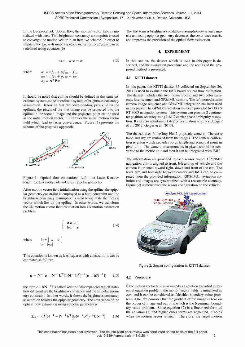
The information are provided in each sensor frame; GPS/IMUnavigation unit is aligned to front, left and up of vehicle and thecamera is oriented toward right, down and front of the car. Thelever arm and boresight between camera and IMU can be com-puted from the provided information. GPS/IMU navigation so-lution and images are synchronized with a reasonable accuracy.Figure (2) demonstrates the sensor configuration on the vehicle.

Figure 2: Sensor configuration in KITTI dataset

4.2 Procedure

If the motion vector field is assumed as a solution to partial differ-ential equation problem, the motion vector fields is initialized aszero and it can be considered as Dirichlet boundary value prob-lem. Also, we consider that the gradient of the image is zero onthe border of image and out of it which is the Neumman bound-ary value problem. Since equation (2) is a linearized form ofthe equation (1) and higher order terms are neglected, it holdswhen the motion vector is small. Therefore, the larger motion



vector can be estimated in a pyramidal scheme. In pyramidalscheme, the image is smoothed and downsampled to lower levelof the pyramid. In the lowest level of the pyramid, the Lucas-Kanade optical flow is employed to estimate the motion vectorfield. Then, the motion vector field is upsampled and it is used asinitial motion vector field in the upper pyramid level. The numberof the levels depend on the maximum motion in the image. Here,5 levels of pyramid has been considered for the images and it hasbeen downsampled and upsampled by 2.

In equation (3), it can be seen that motion vector is estimatedwithin a neighborhood using the Lucas-Kanade optical flow. Thesize of the neighborhood is of importance, the small neighbor-hood leads to more precise optical flow estimation and the largeneighborhood provides more reliable motion vector field. In thispaper, the window size of the optical flow estimation is 17 × 17at the finest level (level 0) and it decreases by 2 per level. There-fore, the window size from finest to coarsest levels of pyramidare 17 × 17, 15 × 15, 13 × 13, 11 × 11, 9 × 9 and 7 × 7. Thishelps us to have lower window size when the image size has beenreduced.

Also, the bilateral filter is employed to increase the precisionof the motion vector field estimation (gaussian filter) and im-prove the estimate of motion vector field at the object boundaries(isotropic filter). The standard deviation for the gaussian filterand isotropic filter are considered as 4 and 50, respectively.

It also should be noted that the fundamental geometry is differ-ent for each level. In other words, the calibration matrix shouldbe downsampled at each level and the fundamental matrix shouldbe constructed for each level. Figure (3) shows the output ofGPS/IMU which explains the dynamic of vehicle along the oper-ation.

(a) a

(b) b

Figure 3: (a) Azimuth (b) Velocity of the vehicle

4.3 Results

The results of the proposed method is shown in Figure (4) andLucas/Kanade optical flow estimation results are given for com-parison purposes. The results are given in four subfigures whichshows the motion vector field between image 0 and image 1, im-age 49 and image 50, image 99 and image 100, and image 149and image 150 for subfigures (a), (b), (c), and (d), respectively.These subfigures include four component. The first component(top-left) shows the overlaid of the previous image on the currentimage where the previous image is in green channel and the cur-rent image is in red channel. The second component (down-left)

shows the reconstructed the current image from the previous im-age using the estimated motion vector field known as warped im-age. The third component illustrates the estimated motion vectorfield using the proposed method and the fourth component showsthe Lucas-Kanade motion vector field. The motion vector field iscolor-coded, that is the direction of the motion vector is shownby color and the brightness of the color indicates the magnitudeof the estimated motion vector.

It should be noted that the warped image has been estimated us-ing the proposed method. In contrast, the warped image usingthe lucas-Kanade method is not given in this paper and the lengthof the paper did not allow us to provide these results. Therefore,the proposed approach and the Lucas-Kanade method has beencompared using the color-coded motion vector field in left com-ponents of each subfigure.

The black regions in warped images has occurred where the warpedimage goes beyond the image boundaries and there is no pixelvalue for those regions of the warped image. It occurs more fre-quently at borders of image where there are many occlusions.Also, the motion vector field estimation is not reliable at the bor-ders of the image since there is not enough information in theneighborhood. The poor estimation of the motion vector fieldlead to some artifacts in warped images.

As can be seen in Figure (3), there is not significant rotation incamera motion and the translation motion is very slow in epoch 0.The left side of subfigure (a) shows that the proposed method hassmoother motion vector field estimation. However, it introducesincorrect motion vector field estimation at the region of the car.The epipolar geometry assumes that the scene is static and themotion is purely due to the camera motion. Therefore, the motionvector field may not be correctly estimated on the moving objectin the scene. As previously motioned, both method show someproblems at the border of the image. In the warped image, thepoorly estimated motion vector field generates some artifact inthe warped image. For instance, the bar of the traffic light is notstraight in the warped image and the incorrect motion vector fieldhas generated artifacts there.

In subfigure (b), the motion vector field has been poorly estimatedin the right side of the image. The right side of the image is verydark and there is very low contrast there. Lack of rich textureleads to ambiguous motion vector field in this part of the image.However, it is clear that the proposed method can handle the tex-tureless regions much better than the Lucas-Kanade optical flowestimation since it exploits the epipolar geometry constraint andit can resolve the ill-conditioned optical flow estimation problemin low contrast and textureless regions.

In subfigure (c) the translational motion of the camera is fasterand motion vector field is larger. Surprisingly, the Lucas-Kanademethod has better performance with respect to the proposed method.For instance, the ground motion (lower part of image) has beenestimated smoother and more realistic in the Lucas-Kanade. Inthe warped image, left side of the image has severely distorted.The optical flow estimation is poor in this region due to very largemotion vector field.

In subfigure (d), there is a large motion in the right side of theimage and the Lucas-Kanade fails to estimated the correct mo-tion, but the proposed method has better estimate of the motionvector field in this region. It can be concluded that the proposedmethod has superior performance over the Lucas-Kanade in largemotion vector field. The warped image displays some artifacts inthe right side of the image due to the occlusion in this part of theimage.



(a)

(b)

(c)

(d)

Figure 4: top left: first and second images are overlaid in different colors; top right: the color coded optical flow LK+epipolar geometryconstraint; down left: warped image LK+epipolar geometry constraint; down right: warped image LK; a, b, c and d are 1, 50, 100 and 150frame numbers in the image sequence



The proposed method can be generalized to the KLT tracker. TheKLT tracker uses the estimated motion vector for interest pointsto locate them in the next image. The KLT tracker uses the bright-ness constancy assumption, but the epipolar geometry can aidthe KLT tracker as explained in this paper. We refer to the KLTtracker aided by epipolar geometry constraint as ”modified KLTtracker” here. Figure (5) shows the modified KLT tracker be-tween image 80 and image 81. Likewise Figure (4), The firstimage in green channel is overlaid on the second image in redchannel.

Seven points has been tracked in a modified KLT tracker andthese points are displayed in small hollow light blue points. Theepiline has been estimated for each of these tracked point usingIMU measurements and it has been displayed in blue line. Theepilines intersect at a point known as epipole. The epipole is thesame as focus of expansion if the motion is translational motionand it lies at the center of the image. However, the epiline is notat the center of the image since the camera has rotation too. It canbe seen in Figure (3).

The projection of these points on the epipolar line is displayed insolid yellow points. Some of the projected points (yellow) cov-ered the tracked points (blue) since the tracked points were closeto the epiline. The proposed method has been used to estimatethe corresponding points in the second image which is shown bysolid red points. Obviously, the epilines pass trough the corre-sponding points (red dots) in the second image. The trackingpoints have been converged to the corresponding points in thesecond image. Therefore, the proposed method can be used insparse correspondence to track the interest points faster and makethem more reliable.

5. CONCLUSION

In this paper, we proposed a method to improve Lucas/Kanadeoptical flow using epipolar geometry constraint. The IMU mea-surement obtains the translation and rotation of the camera expo-sure stations and if the camera is calibrated, the epipolar geome-try can be reconstructed. The brightness constancy assumption inassociation with the epipolar geometry constraint leads to morereliable motion vector field estimation. In the proposed method,first the original point is projected on the epiline and the projectedpoint is used as an initialization point. Then, the epipolar geom-etry constraint and the brightness constancy assumption are usedin a least squares with constraint scheme to estimate the motionvector field.

The KITTI dataset has been used to verify the proposed method.The GPS/IMU measurements are transformed to the camera co-

Figure 5: KLT tracker aided by epipolar geometry constraint

ordinate system. The translation and rotation from GPS/IMU andthe camera calibration are employed to compose the epipolar ge-ometry. Since the motion vector filed is large, it has been esti-mated in a pyramidal scheme. Using the epipolar geometry andbrightness constancy assumption, the motion vector field is es-timated for each pyramid level and the estimated motion vectorfield has been upsample and it has been used as initial motion vec-tor field. The estimated motion vector field in the highest level ofpyramid has been demonstrated in this paper.

The results show that the proposed method can improve the es-timated motion vector field. The proposed method may fail inthe moving object regions since the epipolar geometry constraintassumes that the motion vector field is due to the camera motionand the scene objects are static. On the other hand, the proposedmethod has superior performance in textureless and low contrastregions.

The proposed approach can be used for sparse correspondence.Once the interest points are detected in an image, the proposedmethod can be used to track the interest points in the upcom-ing images. Likewise with the dense correspondence, the interestpoints are projected on the epiline and then brightness constancyassumption and epipolar geometry constraint are used to estimatethe motion vectors and subsequently the corresponding points.

The epipolar geometry constraint can be integrated with a highperformance optical flow estimation. It can be used as an addi-tional term in the optical flow cost function. It has been discussedin the literature, but these papers estimate fundamental matrix inconjunction with the motion vector field and they do not con-sider the IMU measurements to reconstruct the epipolar geome-try. Here, it is suggested that the IMU measurement are employedin motion vector field estimation using variational method.



REFERENCES

Brox, T. and Malik, J., 2011. Large displacement optical flow:Descriptor matching in variational motion estimation. IEEETrans. Pattern Anal. Mach. Intell. 33(3), pp. 500–513.

Brox, T., Bruhn, A., Papenberg, N. and Weickert, J., 2004. Highaccuracy optical flow estimation based on a theory for warping.In: European Conference on Computer Vision (ECCV), Springer,pp. 25–36.

Corke, P., Lobo, J. and Dias, J., 2007. An introduction to inertialand visual sensing. The International Journal of Robotics 26,pp. 519–535.

Geiger, A., Lenz, P. and Urtasun, R., 2012. Are we ready forautonomous driving? the kitti vision benchmark suite. In: Con-ference on Computer Vision and Pattern Recognition (CVPR).

Geiger, A., Lenz, P., Stiller, C. and Urtasun, R., 2013. Vi-sion meets robotics: The kitti dataset. International Journal ofRobotics Research (IJRR).

Horn, B. K. P. and Schunck, B. G., 1981. Determining opticalflow. Artif. Intell. 17(1-3), pp. 185–203.

Javier Sanchez1, E. M.-L. J. S., Meinhardt, E. and Facciolo, G.,2013. TV-L1 Optical Flow Estimation. Image Processing OnLine 3, pp. 137–150.

Jones, E. S. and Soatto, S., 2010. Visual-inertial navigation,mapping and localization: A scalable real-time causal approach.The International Journal of Robotics Research (IJRR) 30(4),pp. 407430.

Joshi, N., Kang, S. B., Zitnick, L. and Szeliski, R., 2010. Imagedeblurring using inertial measurement sensors. In: ACM SIG-GRAPH.

Kelly, J. and Sukhatme, G. S., 2011. Visual-inertial sensor fusion:Localization, mapping and sensor-to-sensor self-calibration. In-ternational Journal of Robotics Research 30(1), pp. 56–79.

Leung, T. and Medioni, G., 2014. Visual navigation aid for theblind in dynamic environments. In: The IEEE Conference onComputer Vision and Pattern Recognition.

Li, M. and Mourikis, A. I., 2013. High-precision, consistent ekf-based visualinertial odometry. International Journal of RoboticsResearch 32(6), pp. 690–711.

Lucas, B. D. and Kanade, T., 1981. An iterative image regis-tration technique with an application to stereo vision. In: Pro-ceedings of the 7th International Joint Conference on ArtificialIntelligence - Volume 2, IJCAI’81, pp. 674–679.

Slesareva, N., Bruhn, A. and Weickert, J., 2005. Optic flow goesstereo: A variational method for estimating discontinuitypreserv-ing dense disparity maps. In: Proc. 27th DAGM Symposium,pp. 33–40.

Szeliski, R., n.d. Computer vision algorithms and applications.Springer, London; New York.

Valgaerts, L., Bruhn, A. and Weickert, J., 2008. A variationalapproach for the joint recovery of the optical flow and the funda-mental matrix. In: Proc. 27th DAGM Symposium, pp. 314–324.

Wedel, A. and Cremers, D., 2011. Stereo Scene Flow for 3DMotion Analysis. Springer.

Zach, C., Pock, T. and Bischof, H., 2007. A duality based ap-proach for realtime tv-l1 optical flow. In: Ann. Symp. GermanAssociation Patt. Recogn, pp. 214–223.



MOTION VECTOR FIELD ESTIMATION USING … · MOTION VECTOR FIELD ESTIMATION USING BRIGHTNESS...

Documents

Transcript of MOTION VECTOR FIELD ESTIMATION USING … · MOTION VECTOR FIELD ESTIMATION USING BRIGHTNESS...