Motion Planning: from Digital Actors to Humanoid Robots
113
HAL Id: tel-00145201 https://tel.archives-ouvertes.fr/tel-00145201 Submitted on 9 May 2007 HAL is a multi-disciplinary open access archive for the deposit and dissemination of sci- entific research documents, whether they are pub- lished or not. The documents may come from teaching and research institutions in France or abroad, or from public or private research centers. L’archive ouverte pluridisciplinaire HAL, est destinée au dépôt et à la diffusion de documents scientifiques de niveau recherche, publiés ou non, émanant des établissements d’enseignement et de recherche français ou étrangers, des laboratoires publics ou privés. Motion Planning: from Digital Actors to Humanoid Robots Claudia Elvira Esteves Jaramillo To cite this version: Claudia Elvira Esteves Jaramillo. Motion Planning: from Digital Actors to Humanoid Robots. Auto- matic. Institut National Polytechnique de Toulouse - INPT, 2007. English. tel-00145201
Transcript of Motion Planning: from Digital Actors to Humanoid Robots

HAL Id: tel-00145201https://tel.archives-ouvertes.fr/tel-00145201
Submitted on 9 May 2007
HAL is a multi-disciplinary open accessarchive for the deposit and dissemination of sci-entific research documents, whether they are pub-lished or not. The documents may come fromteaching and research institutions in France orabroad, or from public or private research centers.
L’archive ouverte pluridisciplinaire HAL, estdestinée au dépôt et à la diffusion de documentsscientifiques de niveau recherche, publiés ou non,émanant des établissements d’enseignement et derecherche français ou étrangers, des laboratoirespublics ou privés.
Motion Planning: from Digital Actors to HumanoidRobots
Claudia Elvira Esteves Jaramillo
To cite this version:Claudia Elvira Esteves Jaramillo. Motion Planning: from Digital Actors to Humanoid Robots. Auto-matic. Institut National Polytechnique de Toulouse - INPT, 2007. English. �tel-00145201�

Ecole Doctorale Systemes
These
pour obtenir le grade de
Docteur de l’Institut National Polytechnique de Toulouse
Specialite: Systemes Informatiques
presentee et soutenue publiquement le 27 fevrier 2007
Motion Planning: from Digital Actors to Humanoid Robots
Claudia Elvira Esteves Jaramillo
Preparee au Laboratoire d’Analyse et d’Architecture des Systemes
sous la direction de M. Jean-Paul Laumond
Jury
M. Franck Multon Rapporteur
M. Yoshihiko Nakamura Rapporteur
M. Nicolas Chevassus Examinateur
M. Marc Renaud Examinateur
M. Eiichi Yoshida Examinateur
M. Jean-Paul Laumond Directeur de These


Abstract
The goal of this work is to develop motion planning algorithms for human-like figures taking into
account the geometry, kinematics and dynamics of the mechanism and its environment.
By motion planning it is understood the ability to specify high-level directives and transform them into
low-level instructions for the articulations of the human-like figure. This is usually done while considering
obstacle avoidance within the environment. This results in one being able to express directives as “carry
this plate from the table to the piano corner” and have them translate into a series of goals and constraints
that result in the pertinent motions from the robot’s articulations in such a way as to carry out the action
while avoiding collisions with the obstacles in the room.
Our algorithms are based on the observation that humans do not plan their exact motions when
getting to a location. We roughly plan our direction and, as we advance, we execute the motions needed
to get to the desired place. This has led us to design algorithms that:
1. Produce a rough collision-free path that takes a simplified model of the mechanism to the desired
location.
2. Use available controllers to generate a trajectory that assigns values to each of the mechanism’s
articulations to follow the path.
3. Modify iteratively these trajectories until all the geometric, kinematic and dynamic constraints of
the problem are satisfied.
Throughout this work, we apply this three-stage approach with the problem of generating motions
for human-like figures that manipulate bulky objects while walking. In the process, several interesting
problems and their solution are brought into focus. These problems are, three-dimensional collision
avoidance, two-hand object manipulation, cooperative manipulation among several characters or robots
and the combination of different behaviors.
The main contribution of this work is the modeling of the automatic generation of cooperative
manipulation motions. This model considers the above difficulties, all in the context of bipedal walking
mechanisms. Three principles inform the model:
– a functional decomposition of the mechanism’s limbs,
– a model for cooperative manipulation and,
– a simplified model to represent the mechanism when generating the rough path.
This work is mainly and above all, one of synthesis. We make use of available techniques for controlling
locomotion of bipedal mechanisms (controllers), from the fields of computer graphics and robotics, and
connect them to a novel motion planner. This motion planner is controller-agnostic, that is, it is able to
produce collision-free motions with any controller, despite whatever errors introduced by the controller
itself. Of course, the performance of our motion planner depends on the quality of the used controller.

In this thesis, the motion planner, connected to different controllers, is used and tested in different
mechanisms, both virtual and physical. This in the context of different research projects in France,
Russia and Japan, where we have provided the motion planning framework to their controllers. Several
papers in peer-reviewed international conferences have resulted from these collaborations. The present
work compiles these results and provides a more comprehensive and detailed depiction of the system and
its benefits, both when applied to different mechanisms and compared to alternative approaches.

Resume
Le but de ce travail est de developper des algorithmes de planification de mouvement pour des figures
anthropomorphes en tenant compte de la geometrie, de la cinematique et de la dynamique du mecanisme
et de son environnement.
Par planification de mouvement, on entend la capacite de donner des directives a un niveau eleve
et de les transformer en instructions de bas niveau qui produiront une sequence de valeurs articulaires
qui reproduissent les mouvements humains. Ces instructions doivent considerer l’evitement des obstacles
dans un environnement qui peut etre plus au moins contraint. Ceci a comme consequence que l’on peut
exprimer des directives comme “porte ce plat de la table jusqu’ac’estu coin du piano”, qui seront ensuite
traduites en une serie de buts intermediaires et de contraintes qui produiront les mouvements appropries
des articulations du robot, de facon a effectuer l’action demandee tout en evitant les obstacles dans la
chambre.
Nos algorithmes se basent sur l’observation que les humains ne planifient pas des mouvements precis
pour aller a un endroit donne. On planifie grossierement la direction de marche et, tout en avancant, on
execute les mouvements necessaires des articulations afin de nous mener a l’endroit voulu. Nous avons
donc cherche a concevoir des algorithmes au sein d’un tel paradigme, algorithmes qui:
1. Produisent un chemin sans collision avec une version reduite du mecanisme et qui le menent au
but specifie.
2. Utilisent les controleurs disponibles pour generer un mouvement qui assigne des valeurs a chacune
des articulations du mecanisme pour suivre le chemin trouve precedemment.
3. Modifient iterativement ces trajectoires jusqu’a ce que toutes les contraintes geometriques,
cinematiques et dynamiques soient satisfaites.
Dans ce travail nous appliquons cette approche a trois etages au probleme de la planification de
mouvements pour des figures anthropomorphes qui manipulent des objets encombrants tout en marchant.
Dans le processus, plusieurs problemes interessants, ainsi que des propositions pour les resoudre, sont
presentes. Ces problemes sont principalement l’evitement tri-dimensionnel des obstacles, la manipulation
des objets a deux mains, la manipulation cooperative des objets et la combinaison de comportements
heterogenes.
La contribution principale de ce travail est la modelisation du probleme de la generation automatique
des mouvements de manipulation et de locomotion. Ce modele considere les difficultes exprimees ci-
dessus, dans les contexte de mecanismes bipedes. Trois principes fondent notre modele:
– une decomposition fonctionnelle des membres du mecanisme,
– un modele de manipulation cooperative et,
– un modele simplifie des facultes de deplacement du mecanisme dans son environnement.
Ce travail est principalement et surtout, un travail de synthese. Nous nous servons des techniques
disponibles pour commander la locomotion des mecanismes bipedes (controleurs) provenant soit de
l’animation par ordinateur, soit de la robotique humanoıde, et nous les relions dans un planificateur
des mouvements original. Ce planificateur de mouvements est agnostique vis-a-vis du controleur utilise,
c’est-a-dire qu’il est capable de produire des mouvements libres de collision avec n’importe quel controleur
tandis que les entrees et sorties restent compatibles. Naturellement, l’execution de notre planificateur
depend en grand partie de la qualite du controleur utilise.
Dans cette these, le planificateur de mouvement est relie a differents controleurs et ses bonnes
performances sont validees avec des mecanismes differents, tant virtuels que physiques. Ce travail a
ete fait dans le cadre des projets de recherche communs entre la France, la Russie et le Japon, ou noust
avons fourni le cadre de planification de mouvement a ses differents controleurs. Plusieurs publications
issues de ces collaborations ont ete presentees dans des conferences internationales. Ces resultats sont
compiles et presentes dans cette these, et le choix des techniques ainsi que les avantages et inconvenients
de notre approche sont discutes.

to Tere
for her example and courage

Acknowledgements
Many people have contributed in some way to this thesis, and I would like to express my deepest
gratitude to them.
First of all, I would like to thank Jean-Paul Laumond, the best advisor I could have wished
for, and without whose efforts for giving clear and simple explanations, his knowledge, criticism
and humor it would have been a much more difficult, if not impossible, task.
I wish to thank Eiichi Yoshida for his help, advise, enthusiasm and hard work carried out
even long-distance.
My thanks to the successive directors of the LAAS-CNRS, Malik Ghallab and Raja Chatila
for providing the facilities for conducting this research.
I wish to express my sincere gratitude to Yoshihiko Nakamura, Frank Multon and Marc
Renaud, for agreeing to be part of my committee and for their valuable suggestions for the
improvement of this work.
Thanks to the people with whom I had the chance to collaborate during these years,
Igor Belousov, Julien Pettre, Gustavo Arechavaleta, Wael Suleiman, Olivier Stasse and to the
Gepettistes, Florent, Anthony, Oussama, Matthieu ...
Thanks to the Kineo crowd, Etienne, Nicolas, Guillaume for always taking the time to answer
my questions and give good ideas.
A very special thanks to Katzuhito Yokoi and Abderrahmane Kheddar, as well as the JRL
(France and Japan) for giving me the incredible opportunity of working with HRP-2 (10 and
14). I am very thankful for the great experience this has been, not only from the scientific point
of view but also for the personal one given the cultural exchange.
I would like to thank the various people who have provided their valuable assistance, a helpful
or encouraging word during these years. Michel Devy, Fred Lerasle, Georges Giralt, Sara Fleury,
Matthieu Herrb, Rafael Murrieta, Steve LaValle, Juan Cortes.
Thanks to my office colleagues and friends for putting up with me all this time: Gustavo,
Thierry, Olivier, Oussama, for making even the hottest days livable ;-)
Thanks a lot to “les enfants”: Nacho, Luis, Thierry and Akin for always being there for me.
I am indebted to my many colleagues for providing a stimulating and fun environment, as
well as for all their help and friendship: Wael, Paulo, Efrain, Aurelie, Joan, Felipe, Sylvain,
Leonard, Jerome, Martial, Anis and all those who I might be forgetting.
I gratefully acknowledge the Mexican National Science and Technology Counsel (CONACyT)
for its financial support during my stay in France.

Acknowledgements · 9
My deepest thanks to Jib, for not only proof-reading this work but for his constant support
and encouragement.
It is difficult to overstate my gratitude to my family, specially to my parents, my brother
Gabriel and my sister Alex, if I am here it is certainly because of them. Thanks.
9

10 · Motion Planning: from Digital Actors to Humanoid Robots
10

Contents
1 Introduction 3
1.1 Contribution of this work . . . . . . . . . . . . . . . . . . . . . . . . . . . . . . . 6
1.2 Document organization . . . . . . . . . . . . . . . . . . . . . . . . . . . . . . . . 7
1.3 Publications associated to this work . . . . . . . . . . . . . . . . . . . . . . . . . 8
2 Sampling-based Motion Planning 9
2.1 The Piano Mover’s Problem . . . . . . . . . . . . . . . . . . . . . . . . . . . . . . 9
2.2 Sampling-based motion planning . . . . . . . . . . . . . . . . . . . . . . . . . . . 10
2.2.1 Visibility PRM . . . . . . . . . . . . . . . . . . . . . . . . . . . . . . . . . 11
2.2.2 Iterative Diffusion Algorithm . . . . . . . . . . . . . . . . . . . . . . . . . 13
2.3 Planning with spatial and kinematic constraints . . . . . . . . . . . . . . . . . . . 14
2.3.1 Closed-kinematic chains . . . . . . . . . . . . . . . . . . . . . . . . . . . . 15
2.3.2 Multiple robots . . . . . . . . . . . . . . . . . . . . . . . . . . . . . . . . . 16
2.3.3 Steering methods . . . . . . . . . . . . . . . . . . . . . . . . . . . . . . . . 17
2.4 From paths to trajectories . . . . . . . . . . . . . . . . . . . . . . . . . . . . . . . 18
2.5 Conclusion . . . . . . . . . . . . . . . . . . . . . . . . . . . . . . . . . . . . . . . 19
3 Humanoid Representation 21
3.1 Hierarchical articulated figures . . . . . . . . . . . . . . . . . . . . . . . . . . . . 22
3.1.1 Direct kinematics . . . . . . . . . . . . . . . . . . . . . . . . . . . . . . . . 23
3.1.2 Inverse kinematics . . . . . . . . . . . . . . . . . . . . . . . . . . . . . . . 25
3.2 Functional decomposition . . . . . . . . . . . . . . . . . . . . . . . . . . . . . . . 27
3.3 Cooperative manipulation model . . . . . . . . . . . . . . . . . . . . . . . . . . . 28
3.4 Motion planning model . . . . . . . . . . . . . . . . . . . . . . . . . . . . . . . . 30
3.5 Conclusion . . . . . . . . . . . . . . . . . . . . . . . . . . . . . . . . . . . . . . . 31
4 Digital Actors: Eugene & Co. 33
4.1 Animation techniques . . . . . . . . . . . . . . . . . . . . . . . . . . . . . . . . . 34
4.1.1 Geometric and kinematic methods . . . . . . . . . . . . . . . . . . . . . . 34
4.1.2 Physical methods . . . . . . . . . . . . . . . . . . . . . . . . . . . . . . . . 36
4.1.3 Behavioral methods . . . . . . . . . . . . . . . . . . . . . . . . . . . . . . 36
4.2 Motion planners for virtual characters . . . . . . . . . . . . . . . . . . . . . . . . 37
i

ii · Motion Planning: from Digital Actors to Humanoid Robots
4.2.1 Motion planning for walking characters . . . . . . . . . . . . . . . . . . . 37
4.2.2 Motion planning for object manipulation . . . . . . . . . . . . . . . . . . 37
4.2.3 Combining behaviors . . . . . . . . . . . . . . . . . . . . . . . . . . . . . . 39
4.3 Our approach . . . . . . . . . . . . . . . . . . . . . . . . . . . . . . . . . . . . . . 39
4.3.1 The motion planner . . . . . . . . . . . . . . . . . . . . . . . . . . . . . . 39
4.3.2 The behavior controllers . . . . . . . . . . . . . . . . . . . . . . . . . . . . 40
4.3.3 The algorithm . . . . . . . . . . . . . . . . . . . . . . . . . . . . . . . . . 42
4.4 Results and discussion . . . . . . . . . . . . . . . . . . . . . . . . . . . . . . . . . 49
4.4.1 Eugenio, “el Mariachi” . . . . . . . . . . . . . . . . . . . . . . . . . . . . . 49
4.4.2 Pizza delivery service . . . . . . . . . . . . . . . . . . . . . . . . . . . . . 49
4.4.3 In the factory . . . . . . . . . . . . . . . . . . . . . . . . . . . . . . . . . . 52
4.4.4 Buren’s Columns . . . . . . . . . . . . . . . . . . . . . . . . . . . . . . . . 53
4.4.5 Transporting the Piano . . . . . . . . . . . . . . . . . . . . . . . . . . . . 54
4.4.6 Computational time . . . . . . . . . . . . . . . . . . . . . . . . . . . . . . 54
4.5 Conclusion . . . . . . . . . . . . . . . . . . . . . . . . . . . . . . . . . . . . . . . 56
5 Motion planning with dynamic constraints 59
5.1 Available techniques . . . . . . . . . . . . . . . . . . . . . . . . . . . . . . . . . . 60
5.1.1 Decoupled trajectory planning . . . . . . . . . . . . . . . . . . . . . . . . 60
5.1.2 Kinodynamic motion planning . . . . . . . . . . . . . . . . . . . . . . . . 61
5.2 Our approach . . . . . . . . . . . . . . . . . . . . . . . . . . . . . . . . . . . . . . 62
5.3 Quasi-static mechanisms . . . . . . . . . . . . . . . . . . . . . . . . . . . . . . . . 64
5.3.1 Workout example: Buran . . . . . . . . . . . . . . . . . . . . . . . . . . . 64
5.3.2 The kinematic path . . . . . . . . . . . . . . . . . . . . . . . . . . . . . . 64
5.3.3 Dynamic motion generation . . . . . . . . . . . . . . . . . . . . . . . . . . 65
5.3.4 Temporal reshaping method . . . . . . . . . . . . . . . . . . . . . . . . . . 66
5.3.5 Simulation Results . . . . . . . . . . . . . . . . . . . . . . . . . . . . . . . 68
5.4 Conclusion . . . . . . . . . . . . . . . . . . . . . . . . . . . . . . . . . . . . . . . 70
6 Humanoid Robots: HRP-2 71
6.1 Related work and contribution . . . . . . . . . . . . . . . . . . . . . . . . . . . . 73
6.2 Our approach . . . . . . . . . . . . . . . . . . . . . . . . . . . . . . . . . . . . . . 74
6.2.1 Kinematic path planner . . . . . . . . . . . . . . . . . . . . . . . . . . . . 76
6.2.2 Dynamic pattern generator . . . . . . . . . . . . . . . . . . . . . . . . . . 77
6.2.3 Smooth spatial reshaping . . . . . . . . . . . . . . . . . . . . . . . . . . . 78
6.3 Simulation and experimental results . . . . . . . . . . . . . . . . . . . . . . . . . 82
6.3.1 Simulation results . . . . . . . . . . . . . . . . . . . . . . . . . . . . . . . 82
6.3.2 Experimental results . . . . . . . . . . . . . . . . . . . . . . . . . . . . . . 83
6.4 Conclusion . . . . . . . . . . . . . . . . . . . . . . . . . . . . . . . . . . . . . . . 86
7 Conclusion: from functional decomposition to whole-body motion 89
ii

Instructions for climbing a staircase
“No one will have failed to observe that frequently the floor bends in such a way that
one part rises at a right angle to the plane formed by the floor and the following section
arranges itself parallel to the flatness, so as to provide a step to a new perpendicular,
a process which is repeated in a spiral or in a broken line to highly variable elevations.
Ducking down and placing the left hand on one of the vertical parts and right hand
upon the corresponding horizontal, one is in momentary possesion of a step or stair.
Each one of these steps, formed as we have seen by two elements, is situated somewhat
higher and further than the prior, a principle which gives the idea of a staircase, while
whatever other combination, producing perhaps more beautiful or picturesque shapes,
would surely be incapable of translating one from the ground floor to the first floor.
You tackle a stairway face on, for if you try it backwards or sideways, it ends up being
particularly uncomfortable. The natural stance consists of holding oneself upright,
arms hanging easily at the sides, head erect but not so much so that the eyes no
longer see the steps immediately above, while one tramps up, breathing lightly and
with regularity. To climb a staircase one begins by lifting that part of the body located
below and to the right, usually encased in leather or deerskin, and which, with a few
exceptions, fits exactly on the stair. Said part set down on the first step (to abbreviate
we shall call it the “foot”), one draws up the equivalent part on the left side (also
called “foot” but not to be confused with the foot cited above), and lifting this other
part to the level of the foot, makes it continue along until it is set in place on the
second step, at which point the foot will rest, and the foot will rest on the first. (The
first steps are always the most difficult, until you acquire the necessary coordination.
The coincidence of names between the foot and the foot makes the explanaition more
difficult. Be especially careful not to raise, at the same time, the foot and the foot.)
Having arrived by this method at the second step, it’s easy enough to repeat the
movements alternately, until one reaches the top of the staircase. One gets off it
easily, with a light tap of the heel to fix it in place, to make sure it will not move until
one is ready to come down.”
Julio Cortazar –“Historia de Cronopios y Famas”, 1962

2 · Motion Planning: from Digital Actors to Humanoid Robots
2

1Introduction
When moving from one place to another we are often unaware of the exact movements of our
arms and legs. So unconscious are these motions that our mind is free to occupy itself with
other things while walking. Mechanical movement in animals and humans is the result of more
than a hundred million years of evolution, and after a relatively extended learning period, most
people master it. Once at this stage, it is often sufficient for us to choose a destination for our
nervous system to automatically direct our limbs into performing the motions that will take us
there.
Humans as a species take this process for granted to such an extent that it was not until
comparatively recently in the History of Philosophy that this problem has warranted special
attention. And it was not until the Enlightenment that the mechanical nature of these motions
was fully accepted. Scholars during this period put forth the notion of a human being as
essentially a “ghost in a machine”, a mind locked inside a device that was subject to the same
mechanical laws as the rest of Nature, and, in particular, the human-made contraptions so in
vogue at the time.
The construction of machines that mimic human movement has a long tradition, with
expressions in myth and art. From the stories of animated statues to the ingenious devices
of the 18th century, the reproduction of human motion has fascinated human kind. Along
with this fascination, came the growing awareness of the complexity of this motion, and the
difficulty of its exact reproduction. Modern physiology describes the involved array of muscles
that, grafted on the skeleton, effect the movements on the bones that result in motion. The
operation of these muscles is highly organized, and requires a control so precise that, from the
engineering standpoint, the human body and its motion is one of the most complicated machines
3

4 · Motion Planning: from Digital Actors to Humanoid Robots
in existence.
The modeling of such a device is not straightforward. The system of interlocking levers
and pulleys that is the muscle-skeletal system is made up of many masses, articulated at joints
that allow a large range and flexibility of movement. The mathematical representation of such
systems is by no means simple; the design of a controller that automatically directs a system
like this into performing the motions that we see as natural in the human body is a task of
such proportion that it draws upon numerous research fields and has outright created others.
Foremost among these are the areas of animation and humanoid robotics, which shall be explored
to some extent in this thesis.
Both these fields approach the problem of human motion imitation in similar ways, and
although their stated aims differ considerably, the boundaries between them are increasingly
blurry. Animation mainly occupies itself with the synthesis of anthropomorphic motion of virtual
characters for on-screen performance. These characters become more and more detailed as the
field of animation morphs into that of simulation. In Simulation, more precise representations
of the characters and their environment are needed. Further towards the realistic end of the
spectrum, humanoid robotics are more or less accurate simulacra of the human body, inasmuch
as articulation is concerned, and the environment they are to operate is no mock-up, but the
world itself.
Animation
It is not adventurous to say that computer animation for virtual characters was created to
lighten the animator’s burden of specifying the precise movements that the character has to
perform when going from one place to another. This allows the animator to focus on the details
relevant to the scene, leaving the rest of the motion to be computed automatically. There are
forms of animation, like stop-motion techniques, in which is precisely in this exact description
of the motions where the art resides, but we will not consider them in this work.
Computer animation of anthropomorphic characters forms the core of three applications:
animated films, real-time applications and simulation. Their common goal is the generation of
realistic human-like motions. It is in the meaning of “realistic” where the difference between
applications lies. In the case of entertainment, endowing the synthetic characters in a movie
with movement that is eye-believable is sufficient, and constraints are often relaxed in favor
of higher performance or other considerations. In simulation applications, movements have, in
addition, to obey the laws of physics, in particular conservation principles, as the purpose is to
gain insight into how processes occur in the real world.
The main difficulty when generating eye-believable motions is that, as we are very familiar
with our own, any artifact, however small, draws our attention immediately. For this reason,
motion-capture techniques that record the movements from real actors and adapt them to the
virtual character are frequently used. These, together with editing techniques, are used to
generate the high quality human-like motions required in films and video games.
Other methods to produce motions for virtual characters, such as the dynamic simulation of
4

Introduction · 5
the forces driving the human body or inverse kinematics can also be used. Although it is unlikely
that at their current state of development any of these techniques replaces motion capture
completely, they still draw considerable attention. This situation is due to a number of factors.
Considerable extra information on the human body, for example new biomechanical models,
can be brought into play. Also, these methods allow more control to the sequences. Lastly,
more powerful hardware provides for the computing-intensive aspects of these methods. The
combination of these circumstances result in constantly improving methods, which, furthermore,
do not exclude the possibility of incorporating recorded data from motion capture, for much
enhanced motion sequences.
Robotics
In contrast to computer animation, motion captured data is used in humanoid robotics mostly
in a supporting role, only to enhance the natural appearance of the motions synthesized by other
methods. Humanoid robotics is concerned with producing physically feasible movements, and
for this, inverse kinematics and dynamic simulation are as yet unsurpassed.
As it has been extensively proved in engineering, building machines on the same principles
Nature uses for an equivalent function is not necessarily the best approach. For instance, the
best flying device yet, the airplane, does not use beating wings like the birds do. This begs the
question, why make robots that resemble humans?
The creation of humanoid robots has been motivated by the idea of having a device capable of
operating in environments made by and for humans with minimal change to those environments.
These machines are expected to perform autonomously most of the functions a person is capable
of. These include climbing stairs, reaching for objects, carrying stuff, etc.
Among the researchers in humanoid robotics, two main streams of thought can be identified.
The first aims at producing machines that help people with reduced mobility in their households
without the need to change their environment to suit the robot’s features. The second claims
that, independently of their application, the humanoid robot represents an excellent integration
framework for new technologies.
The former school has found its base mainly in Japan. Since the last decade, growing interest,
not only from universities but also from industries and even from the government have turned
humanoid robotics into a vibrant area of research. Testament of this is the constant stream of
applications and increasingly impressive exhibition models, like Asimo or HRP-2. At this stage,
their main application is in entertainment, but these robots are rapidly maturing towards their
role of human aids.
The second school places the emphasis of the field of humanoid robotics on its research
potential. Humanoid robots constitute a fantastic platform for testing and validating algorithms
in a wide spectrum of research fields. A humanoid robot is a system where hardware and
software coalesce into an agent able to perceive its environment, to formulate plans to achieve
its goals in this environment, and to take action to implement these plans. This perception-
planification-action paradigm makes intensive use of sensor data processing, artificial intelligence,
5

6 · Motion Planning: from Digital Actors to Humanoid Robots
motion planning algorithms, etc. A growing area of concern is the operation of this paradigm
in a changing environment, where adaptation is key. It is in this context that behavioral
approaches and learning techniques may be used, making humanoid platforms also appealing to
neuroscientists and psychologists.
The work and early successes of the field has brought back the age-old distaste for human
simulacra. The idea, widespread in science fiction and popular culture, that humanoid robots
will at some point become a stronger, smarter version of human beings, able and willing to
control, enslave or replace its designers, is nowhere close to the intentions of any research group.
The prospect of such a device becoming a reality is, in fact, far from feasible in the short run,
and unlikely even in the far future.
Although computer animation of human-like figures and humanoid robotics have used the
same representation for quite some time, interaction among these fields has been rare up till
the past few years. Both of these areas have reached a point where techniques developed for
humanoid robots can be applied to virtual characters without jeopardizing the naturalness of the
movements generated by computer animation techniques. Likewise, techniques from computer
animation are able to handle constraints in such a way that the motions remain physically
feasible. This has made researchers in both areas become more and more interested in each
others’ methods, making the frontier increasingly blurry. It is in this area of intersection where
the major contribution of this thesis places itself.
1.1 Contribution of this work
The goal of this thesis is to develop motion planning algorithms for human-like figures that take
into account the geometry, kinematics and dynamics of the mechanism and its environment.
By motion planning it is understood the ability to specify high-level directives and transform
them into low-level instructions for the articulations of the human-like figure. This is usually
done while considering obstacle avoidance in the environment. This results in one being able to
express directives as “carry this plate from the corner to the table” and have them translate into
a series of goals and constraints that result in the pertinent motions from the robot’s articulations
in such a way as to carry out the action while avoiding collisions with the obstacles in the room.
Our algorithms are based on the observation that humans do not plan their exact motions
when getting to a location. We roughly plan our direction and, as we advance, we execute the
motions needed to get to the desired place. This has led us to design algorithms that:
1. Produce a rough collision-free path that takes a simplified model of the mechanism to the
desired location.
2. Use available controllers to generate a trajectory that assigns values to each of the
mechanism’s articulations to follow the path.
3. Modify iteratively these trajectories until all the geometric, kinematic and dynamic
constraints of the problem are satisfied.
6

Introduction · 7
Throughout this work, we apply this three-stage approach with the problem of generating
motions for human-like figures that manipulate bulky objects while walking. In the process,
several interesting problems and their solution are brought into focus. These problems are,
three-dimensional collision avoidance, two-hand object manipulation, cooperative manipulation
among several characters or robots and the combination of different behaviors.
The main contribution of this work is the modeling of the automatic generation of cooperative
manipulation motions. This model considers the above difficulties, all in the context of bipedal
walking mechanisms. Three principles inform the model:
– a functional decomposition of the mechanism’s limbs,
– a model for cooperative manipulation and,
– a simplified model to represent the mechanism when generating the rough path.
This work is mainly and above all, one of synthesis. We make use of available techniques for
controlling locomotion of bipedal mechanisms (controllers), from the fields of computer graphics
and robotics, and connect them to a novel motion planner. This motion planner is controller-
agnostic, that is, it is able to produce collision-free motions with any controller, despite whatever
errors introduced by the controller itself. Of course, the performance of our motion planner
depends on the quality of the used controller.
In this thesis, the motion planner, connected to different controllers, is used and tested in
different mechanisms, both virtual and physical. This in the context of different research projects
in France, Russia and Japan, where we have provided the motion planning framework to their
controllers. Several papers in peer-reviewed international conferences have resulted from these
collaborations. The present work compiles these results and provides a more comprehensive and
detailed depiction of the system and its benefits, both when applied to different mechanisms
and compared to alternative approaches.
1.2 Document organization
This document is divided in seven chapters in the following way: In Chapter 2 we present a
general overview of probabilistic motion planning methods, which serve as basis for this work.
Here, we describe some of the techniques to deal with geometric and kinematic constraints,
which represent the bulk of the developments in Motion Planning.
Chapter 3 depicts the modeling of the mechanism and the three underlying principles of
our motion planner. Here, we describe part of the contribution of this work: the functional
decomposition of the articulated figure, the model of cooperative tasks and the construction of
a simplified system that represents the stated problem.
In Chapter 4 we present a strategy for planning the motions of one or more virtual characters
constrained only by kinematics. This part of our work illustrates mainly our model of cooperative
manipulation of walking characters. Here, the eye-believability of the motions takes the center
stage.
7
8 · Motion Planning: from Digital Actors to Humanoid Robots
Chapters 5 and 6 puts the spotlight on the dynamic constraints in motion planning. Chapter
5 introduces our algorithm in the context of quasi-static mechanisms. This are mechanisms which
can move arbitrarily slowly. Chapter 6 extends the applicability of the algorithm to mechanisms
with more complicated behavior. In particular we deal with the humanoid robot HRP-2, a
mechanism whose dynamic constraints cannot be reduced.
Chapter 7 concludes and sketches ongoing and future lines of research.
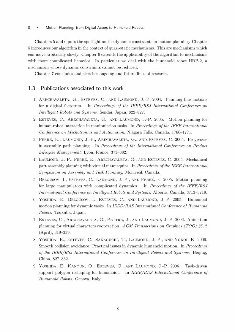
1.3 Publications associated to this work
1. Arechavaleta, G., Esteves, C., and Laumond, J.-P. 2004. Planning fine motions
for a digital factotum. In Proceedings of the IEEE/RSJ International Conference on
Intelligent Robots and Systems. Sendai, Japan, 822–827.
2. Esteves, C., Arechavaleta, G., and Laumond, J.-P. 2005. Motion planning for
human-robot interaction in manipulation tasks. In Proceedings of the IEEE International
Conference on Mechatronics and Automation. Niagara Falls, Canada, 1766–1771.
3. Ferre, E., Laumond, J.-P., Arechavaleta, G., and Esteves, C. 2005. Progresses
in assembly path planning. In Proceedings of the International Conference on Product
Lifecycle Management. Lyon, France, 373–382.
4. Laumond, J.-P., Ferre, E., Arechavaleta, G., and Esteves, C. 2005. Mechanical
part assembly planning with virtual mannequins. In Proceedings of the IEEE International
Symposium on Assembly and Task Planning. Montreal, Canada.
5. Belousov, I., Esteves, C., Laumond, J.-P., and Ferre, E. 2005. Motion planning
for large manipulators with complicated dynamics. In Proceedings of the IEEE/RSJ
International Conference on Intelligent Robots and Systems. Alberta, Canada, 3713–3719.
6. Yoshida, E., Belousov, I., Esteves, C., and Laumond, J.-P. 2005. Humanoid
motion planning for dynamic tasks. In IEEE/RAS International Conference of Humanoid
Robots. Tsukuba, Japan.
7. Esteves, C., Arechavaleta, G., Pettre, J., and Laumond, J.-P. 2006. Animation
planning for virtual characters cooperation. ACM Transactions on Graphics (TOG) 25, 2
(April), 319–339.
8. Yoshida, E., Esteves, C., Sakaguchi, T., Laumond, J.-P., and Yokoi, K. 2006.
Smooth collision avoidance: Practical issues in dynamic humanoid motion. In Proceedings
of the IEEE/RSJ International Conference on Intelligent Robots and Systems. Beijing,
China, 827–832.
9. Yoshida, E., Kanoun, O., Esteves, C., and Laumond, J.-P. 2006. Task-driven
support polygon reshaping for humanoids. In IEEE/RAS International Conference of
Humanoid Robots. Genova, Italy.
8
“Odd, I’ve certainly never come across any irreversible mathematics
involving sofas. Could be a new field. Have you spoken to any spatial
geometricians?”
Douglas Adams – Dirk Gently’s Holistic Detective Agency.
2Sampling-based Motion Planning
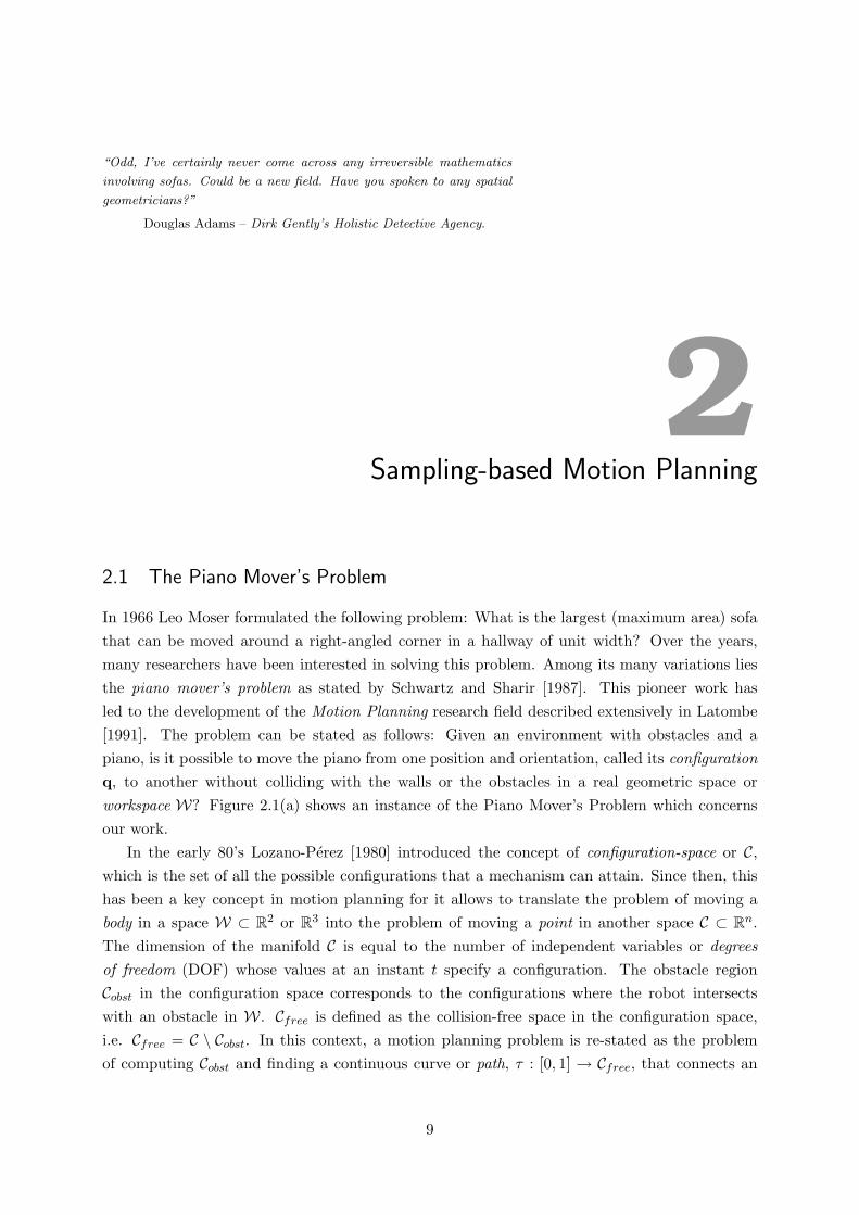
2.1 The Piano Mover’s Problem
In 1966 Leo Moser formulated the following problem: What is the largest (maximum area) sofa
that can be moved around a right-angled corner in a hallway of unit width? Over the years,
many researchers have been interested in solving this problem. Among its many variations lies
the piano mover’s problem as stated by Schwartz and Sharir [1987]. This pioneer work has
led to the development of the Motion Planning research field described extensively in Latombe
[1991]. The problem can be stated as follows: Given an environment with obstacles and a
piano, is it possible to move the piano from one position and orientation, called its configuration
q, to another without colliding with the walls or the obstacles in a real geometric space or
workspace W? Figure 2.1(a) shows an instance of the Piano Mover’s Problem which concerns
our work.
In the early 80’s Lozano-Perez [1980] introduced the concept of configuration-space or C,
which is the set of all the possible configurations that a mechanism can attain. Since then, this
has been a key concept in motion planning for it allows to translate the problem of moving a
body in a space W ⊂ R2 or R
3 into the problem of moving a point in another space C ⊂ Rn.
The dimension of the manifold C is equal to the number of independent variables or degrees
of freedom (DOF) whose values at an instant t specify a configuration. The obstacle region
Cobst in the configuration space corresponds to the configurations where the robot intersects
with an obstacle in W. Cfree is defined as the collision-free space in the configuration space,
i.e. Cfree = C \ Cobst. In this context, a motion planning problem is re-stated as the problem
of computing Cobst and finding a continuous curve or path, τ : [0, 1] → Cfree, that connects an
9

10 · Motion Planning: from Digital Actors to Humanoid Robots
(a) (b)
Figure 2.1: (a) Our version of the Piano Mover’s Problem. Two robots and a virtual character cooperateto transport a piano in a workspaceW ⊂ R
3. (b) The configuration space is divided in Cfree (light areas)and Cobst (dark areas). A path can be found between q1 and q2 because they lie in the same connectedcomponent of Cfree, which is not the case for q3.
initial configuration τ(0) = qinit to a final configuration τ(1) = qend. A path exists if and only
if qinit and qend belong to the same connected component1 of Cfree (see Figure 2.1(b)).
During the following years, several planners that constructed an explicit and exact
representation of Cobst were described in the literature e.g. [Schwartz and Sharir 1987; Goodman
and O’Rourke 2004; Canny 1988]. These kind of methods rely on exact cell decompositions,
visibility graphs and Voronoi diagrams [Latombe 1991] to construct a graph in Cfree, called
roadmap which is accessible from any q ∈ Cfree allowing to find a path that connects qinit to
qend if one exists. Although these approaches have desirable properties such as completeness2,
the combinatorial complexity is such, that it makes even simple problems computationally
intractable.
In order to provide a practical resolution for the planning problem, sampling-based methods
have been developed over the last decade. Although these methods involve a weaker form of
completeness, they have proven their efficacy for solving difficult problems in high-dimensional
spaces, such as the ones addressed in the present work.
2.2 Sampling-based motion planning
The aim of these approaches is to capture the topology of Cfree in a roadmap RM without
requiring an explicit computation of Cobst. The roadmap is used, as in the combinatorial
approaches, to find a collision-free path that connects qinit to qend. A roadmap can be obtained
1a part of the space that consists in only one component2algorithm’s property which means that it will always find a solution, if one exists, or declare the absence of
it in finite time.
10

Sampling-based Motion Planning · 11
mainly by using two types of algorithms: sampling and diffusion. These methods are said to
be probabilistic complete, which means that the probability of finding a solution, if one exists,
converges to 1 as the computing time tends to infinity.
The main idea of the sampling technique, introduced as PRM or Probabilistic Roadmaps by
Kavraki et al. [1996] and shown in Figure 2.2(a), is to draw random collision-free configurations
lying in Cfree and to trace edges to connect them with its k-neighbor samples. Edges or local
paths L(q, q′) should also be collision-free and their form depends on the kinematic constraints
of the robot or moving device.
The principle of diffusion techniques, usually referred to as Expansive-Space Trees (EST)
[Hsu et al. 1998] or Rapid-Random Trees (RRT) [LaValle 1998], consists in sampling Cfree with
only a few configurations called roots and to diffuse the exploration in the neighborhood to
randomly chosen directions until the goal configuration can be reached (Figure 2.2(b)). Motion
planners using this methods, are called single-query because they are specific to the input
configurations.
When using PRM-like methods, a path is found by using a two-step algorithm consisting of a
learning phase and a query phase. In the learning phase, random configurations are drawn within
the range allowed for each degree of freedom of the mechanism in order to build a probabilistic
roadmap. In the query phase, the initial and final configurations are added as new nodes in
the roadmap and connected with collision-free edges. Then, a graph search is performed to find
a collision-free path between the start and goal configurations. If a path is found, then it is
smoothened to remove useless detours. Finally, it is converted into a time-parameterized path
or trajectory τ(t) by means of classical techniques [Shin and McKay 1985; Bobrow et al. 1985;
Slotine and Yang 1989; Renaud and Fourquet 1992; Lamiraux and Laumond 1998].
2.2.1 Visibility PRM
In this work, as we are dealing with systems with a large number of degrees of freedom (DOFs),
we rely on sampling-based methods for computing our roadmaps. We use in particular a variant
of the PRM method, the Visibility PRM, proposed by Simeon et al. [2000] and despicted in
Figure 2.3.
The main idea of this technique is, as in the basic PRM approach, to capture the topology
of Cfree into a roadmap. The main difference is that not every collision-free drawn node is
integrated into RM but only the nodes with certain visibility or connection characteristics are
added to the roadmap.
The visibility or reachable domain of a randomly sampled configuration q for a given local
method L is defined as:
V isL(q) = {q′ ∈ Cfree such that L(q, q′) ⊂ Cfree} (2.1)
Configuration q is said to be the guard of the visibility domain V isL(q). Figure 2.3 shows a
configuration qg1and its associated visibility domain V isL(qg1
) using a straight line segment as
11

12 · Motion Planning: from Digital Actors to Humanoid Robots
(a)
(b)
Figure 2.2: (a) In the PRM algorithm a roadmap RM is build around the obstacles by drawing randomcollision-free configurations (nodes) and connecting them to their k-nearest neighbors using feasible robotmotions (edges). The query is solved by connecting qinit and qend to the graph and then finding theshortest path on it (thick lines) (b) With the RRT algorithm, two trees rooted on Ts = qinit andTg = qend can be grown simultaneously. Each tree is expanded until leaf configurations q1 and q2 fromeach tree can be connected by a randomly drawn configuration qrand.
12

Sampling-based Motion Planning · 13
Figure 2.3: The Visibility-PRM algorithm produces a compact roadmap around obstacles with only afew nodes: guards qg (dark circles) and connectors qc(in white). A new randomly drawn configurationqrand is added as a guard if it covers a previously unseen visibility domain with a given L or as a connectorif it serves as liaison between at least two connected components.
local method.
A visibility roadmap is then constructed incrementally by adding randomly sampled
configurations that either serve as liaison between two connected components of the roadmap
(connector nodes) or those who are not visible from previously sampled guard nodes. The
roadmap construction is ended when the coverage of Cfree is over a given threshold. The
generated roadmap using the Visibility PRM algorithm is more compact that the one obtained
using PRM alone.
When dealing with complex static environments, this kind of sampling-based method allows
us, to precompute offline a roadmap at the learning phase and then use it to solve multiple
queries, saving time on each query.
2.2.2 Iterative Diffusion Algorithm
In our work we sometimes deal with instances of motion planning for part disassembly or highly
constrained environments. In such cases, diffusion techniques have proven to be more efficient
than PRM-like methods as the latter require a high density of sampled points to naturally find
the narrow passages. When dealing with highly constrained environment we have chosen to
use the iterative diffusion algorithm presented by Ferre and Laumond [2004]. The main idea
of this algorithm is to first compute a path that allows a given value of penetration with the
obstacles and then apply an iterative path-refining stage by decreasing the allowed penetration
13

14 · Motion Planning: from Digital Actors to Humanoid Robots
(a) (b) (c)
(d) (e) (f)
Figure 2.4: (a) A first tree is grown allowing a large value of dynamic penetration δ. (b) Decreasing thevalue of δ local paths are tested for collision and removed if collision is found. (c) A new tree is grownusing the remaining roadmaps and the decreased value of allowed δ. (d) and (e) The process is iterativelyperformed until the tree is entirely in Cfree. (f) A collision-free path is found in the remaining tree fromqinit to qend.
value. The algorithm, depicted in Figure 2.4 is the following: First, a tree is grown using a large
value of dynamic penetration δ. This allows to enlarge narrow passages in order to find a good
approximation of the final collision-free path (Figure 2.4(a)). In a second stage (Figure 2.4(b))
the value of δ is decreased by a given scale factor α and the previously computed local paths
are re-tested for collision. The colliding local paths are removed producing sets of collision-free
nodes linked with collision-free edges (Figures 2.4(b) and (d)) which are given as input to the
next stage. Each further iteration of the algorithm will be strongly speeded up because the new
RRT has to link only the previously computed connected components (Figures 2.4(c) and (e)).
The iterative process is repeated until δ reaches a user-specified value. Finally, a collision-free
path is found to connect the initial configuration qinit with the goal configuration qend.
The effectiveness of a motion planning algorithm depends heavily on how well it considers
not only the constraints imposed by the environment, but also those imposed by the mechanisms
themselves.
2.3 Planning with spatial and kinematic constraints
The addition of the robot’s intrinsic constraints into the motion planning problem, causes the
modification of the search space, which is no longer limited to Cfree as defined before. Now, a
14

Sampling-based Motion Planning · 15
valid configuration is not only the one that is collision-free but also that which satisfies additional
constraints such as closure equations when closed kinematic chains are formed. The applications
considered in this work require the motion planning algorithms to respect several geometric,
kinematic and dynamic constraints.
The following paragraphs describe how these constraints are integrated in the context of
sampling-based approaches.
2.3.1 Closed-kinematic chains
In the applications considered in this work, it is usually the case that a virtual character or
a humanoid robot transports an object with both hands forming a loop. These loops should
remain closed along the entire path.
Some path planning methods that consider closed kinematic chains have been described
recently in the literature [LaValle et al. 1999; Han and Amato 2000; Yakey et al. 2001; Cortes
and Simeon 2005].
In LaValle et al. [1999], sampling is done by ignoring kinematic closure and a gradient descent
is performed to force the configuration to satisfy the closure constraints. Numerical optimization
techniques are used to connect configurations with edges that satisfy the constraints within a
given tolerance. This method is general enough but the convergence of the optimization-based
methods is frequently slow. In Yakey et al. [2001] a method to randomly sample the tangent
space of the constraints to increase the effectiveness of the edge creation procedure is presented.
Han and Amato [2000] described a method where the closed mechanism is divided into two
subchains called active and passive subchains.
Nodes are drawn only for the active subchain and an inverse kinematics algorithm is applied
on the passive part to see if the chain can be closed, verifying the validity of the configuration.
This approach leads to many unfeasible configurations, specially as the size of the active subchain
increases, making the sampling process expensive. Another drawback of this method is that a
closed-form kinematics algorithm is required, making it necessary for the passive subchain to be
non-redundant.
Based on the same principle of breaking the kinematic loop into active and passive
parts, Cortes and Simeon [2005] proposed a planner for closed kinematic chains. Here, the
authors propose a dedicated algorithm, called Random-Loop Generator or RLG, for sampling
configurations of closed-chain mechanisms. The main idea in this algorithm is to progressively
decrease the complexity of the closed kinematic chain by performing a guided random sampling
for the active subchain until only the configuration of the passive subchain remains to be solved
by means of a closed-form inverse kinematics algorithm. This guided random sampling increases
significantly the probability of obtaining configurations that satisfy the closure constraints.
Figure 2.5 [Cortes and Simeon 2005] illustrates the RLG algorithm. Here, the joint variables
of the active subchain are sampled sequentially and the two active portions of the chain (the
two first links on the left side and the first link on the right) are treated alternately. The range
at which each joint is sampled depends on the configuration of the previously processed joints.
15

16 · Motion Planning: from Digital Actors to Humanoid Robots
Figure 2.5: RLG algorithm. Figure taken from Cortes and Simeon [2005]. The closed kinematic chainis broken in two parts, active (dark chain) and passive (light chain). (a) A collision-free configuration isfound for the first link of the active chain taking into account the reachable workspace of the chain thatgoes from joint 6 to joint 2 (RWS(6K2)). (b) and (c) Configurations for the active part are sampledalternately reducing the complexity of the chain at each iteration. (d) An inverse kinematics algorithmis performed on the passive part to close the chain.
This range or reachable workspace (RWS) is approximated by a spherical shell, defined as the
region between two concentric balls of different radii. The parameters to construct this volume
are mainly the origin and the maximum/minimum extensions of the chain. The appropriate
values for the passive subchain are computed by solving an inverse kinematics problem. This
approach has proven to be effective in PRM as well as RRT-based planners.
2.3.2 Multiple robots
Two types of planners that handle the motions of multiple robots sharing the same environment
have been proposed in the literature: centralized and decoupled. In the centralized approach
all the robots present in the environment are considered as a single system. A system’s
configuration considers, thus, the degrees of freedom of all robots simultaneously, resulting
usually in a high-dimensional configuration space. In the decoupled approach, motions for
each robot are computed independently and the interactions among robots are considered in
a second stage. Several solutions have been proposed to solve the interaction problem once a
16

Sampling-based Motion Planning · 17
path is found for each robot. Among these, one has been to assign a priority to each robot and
sequentially compute the paths for the rest of the robots in a time-varying configuration space
(see [Erdmann and Lozano-Perez 1986]). Another solution has been to compute coordination
diagrams [O’Donnell and Lozano-Perez 1989] that represent the configurations along each of the
robot’s paths at which mutual collisions might occur. Planners inspired in this approach have
been presented by [Svestka and Overmars 1995] and [Simeon et al. 2002] among others.
2.3.3 Steering methods
Sampling-based algorithms require a function that connects two random configurations with
paths in Cfree that can be executed by the robot. We refer to these connections as local paths
computed by a so-called steering method. When the mechanism can move instantaneously to
any direction3 (e.g. the piano), every path in Cfree corresponds to a valid collision-free motion in
W; hence straight lines (or geodesics in any surface) are the shortest lenght paths between two
configurations. This is not, however, the case for a large class of systems as for example car-like
systems that allow rolling but are unable to move sideways. This kind of kinematic constraints
which cannot be integrated to be expressed exclusively in terms of the configuration variables
are called nonholonomic constraints. They were introduced in the context of motion planning
in Laumond [1986] and since then have been extensively discussed in [Li and Canny 1992] and
[Laumond et al. 1998] among others.
Nonholonomic constraints arise from the nature of the controls that can be applied to the
system. For instance, the car-like mechanism has two controls (linear and angular velocities)
but it moves in the 3-dimensional configuration space with coordinates (x, y, θ). A solution to
the problem of finding feasible paths for systems with nonholonomic constraints in Cfree consists
in decoupling the problem in two parts.
First, feasible paths are computed in the tangent space of the C-manifold by a steering
method in the absence of obstacles and then, in a second stage they are tested for collision. For
some systems, such as a car that can drive only forwards, minimum-length curves that connect
two configurations in the absence of obstacles have been identified to be a combination of arcs of
circle and straight lines [Dubins 1957]. Shortest paths have also been found for a car that goes
forwards and backwards in [Reeds and Shepp 1990] or for a differential drive car in [Balkcom
and Mason 2002]. Steering methods for other systems such as a car with n-trailers have been
proposed in the literature [Lamiraux and Laumond 2000].
Motion planners for the aforementioned systems (except for the Dubin’s car) rely on the
property of small-time local controllability or STLC, which turns out to be fundamental when
computing motions in the presence of obstacles. This states that a system is small-time local
controllable if the set of points that can be reached from a configuration or state4 x at time
T , are reachable without leaving a neighborhood V . Practically, this means that for small-time
3These mechanisms are said to be holonomic.4assuming that the system is kinematic, which means that the state x in a smooth manifold M is simply a
configuration q ∈ C.
17

18 · Motion Planning: from Digital Actors to Humanoid Robots
Figure 2.6: A system is small-time controllable from x if Reachx(T ) contains a neighborhood of x forall neighborhoods V for any time T > 0. If this is so, the system can be approximated to any τ by a setof feasible maneuvers.
controllable systems, any path τ in Cfree can be decomposed into a set of feasible maneuvers as
long as there exists an arbitrarily small clearance value ǫ around the path as shown in Figure 2.6.
The implications of the STLC property in sample-based algorithms are that the problem
can be decoupled in two: first to solve the geometric problem in the same way as for holonomic
robots, and then to approximate the path by a sequence of admissible paths computed by a
steering method that takes into account the STLC.
Another approach is to use directly a steering method that considers STLC to compute the
edges that link configurations in a probabilistic roadmap framework.
2.4 From paths to trajectories
Most of the methods described above produce a curve τ : [0, 1] → C respecting spatial and
kinematic constraints but does not consider the speed of execution. This is an important issue,
not only to be able to execute planned motions on the real system but also to optimize execution
time. Trajectory planning is thus, the problem of determining a feasible time-parameterized
path τ(t). Two kinds of methods have been used to plan a trajectory: decoupled planning and
direct planning.
In the decoupled approach, a path is first found in the configuration space, and then a
time-optimal time-scaling for the path is found, taking into account the system’s mechanical
limits. This usually involves smoothing the path with canonical geometric curves such as splines.
18

Sampling-based Motion Planning · 19
Examples of decoupled approaches can be found in [Shin and McKay 1985] or [Kanayama and
Miyake 1986] among many others.
In the direct planning approach, a trajectory is found directly in the system’s state space by
using, for instance, optimal control methods, dynamic programming or randomized probabilistic
methods (e.g. in LaValle and Kuffner [2001]). These methods are further discussed in Chapter
5.
2.5 Conclusion
We have presented some of the available techniques for planning the motions of different types of
mechanisms with different types of constraints. This short state of the art is not intended to be
exhaustive but focused on the constraints that we consider on our applications. For this reason,
important axes of the Motion Planning research such as manipulation planning (e.g [Simeon
et al. 2004]) or handling dynamic environments (e.g [van den Berg et al. 2005]) have been left
out. The recent textbooks of Choset et al. [2005] and LaValle [2006] present an extensive state
of the art on Motion Planning.
There is no best technique to solve a motion planning problem and several approaches can
be used to consider a given constraint. The difficulty of the motion planning problem depends
not only on the system’s characteristics but also on how the problem is modeled and which
constraints are taken into account. The more simplified the problem is at the planning step, the
more difficult it will be when trying to execute it, and viceversa.
Important basic remarks for the rest of this work are:
– The environments are static, which means that no moving obstacles are considered.
Nevertheless, our proposed strategy is well adapted for the inclusion of dynamic
environments using existing techniques (e.g. Shiller et al. [2001],van den Berg et al. [2005]).
– The environments are completely known, i.e. no uncertainties are taken into account and
no localization or mapping are performed. In this work, the availability of an exact map
of the environment for the virtual character applications remains a reasonable one. In the
case of the humanoid robot, this point will be treated as future work.
– When we refer to the manipulation behavior we do not imply manipulation planning in the
sense of Simeon et al. [2004], where re-grasping is allowed. In our work, manipulation is
described as the following of a fixed frame on an object with one of the robot’s end-effectors.
Along the next chapters we show and justify our choices of the techniques that we experienced
to be the best adapted to our modeling of the problem.
19

20 · Motion Planning: from Digital Actors to Humanoid Robots
20

“Si (como afirma el griego en el Cratilo) el nombre es arquetipo de la
cosa en las letras de ‘rosa’ esta la rosa y todo el Nilo en la palabra
‘Nilo’.” 1
Jorge Luis Borges – El Golem
3Humanoid Representation
Human figure modeling has been an active area of research in many fields of human knowledge
and artistic expression since ancient times. Given the complexity of the human body it is very
difficult, if not impossible, to include all the motion capabilities and constraints in a single model.
Many types of representations have been used along the centuries, where different characteristics
of the human motion have been enhanced, depending on the representation itself. To deal
with this complexity, a widely-used approach has been to separate the human body into layers
according to its physical organization (see Figure 3.1). This has been useful not only when it
comes to the analysis of the motions (as in kinesiology, neuroscience, etc.) but also when trying
to simulate it (as in computer animation or robotics). To this purpose, motions can be generated
for each layer and then added to produce complex motions.
According to Chadwick et al. [1989], realistic2 motions can be simulated with a computer by
using a four-layered approach. They described four layers:
1. Behavior layer – In this layer the parameters that specify the motions at a control level are
described. These parameters are directly applied when generating the skeleton’s motion.
They include the ‘pose’ or configuration vector q as well as the specification of velocities
and accelerations to execute the motions.
1free tr. “If (as the Greek asserts in the Cratylus) the name is archetype to the thing, in the letters of ‘rose’
the rose exists and all the Nile in the word ‘Nile’.”2 By realistic we understand not only eye-believable, but also physically feasible motion.
21
22 · Motion Planning: from Digital Actors to Humanoid Robots
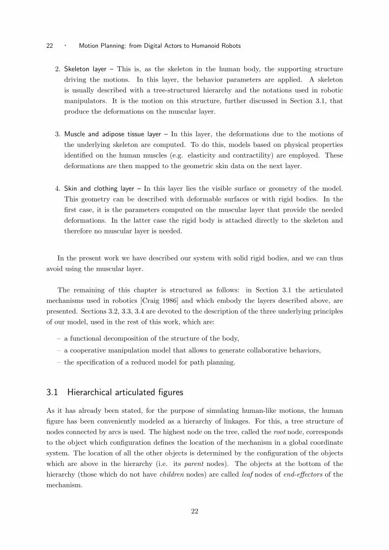
2. Skeleton layer – This is, as the skeleton in the human body, the supporting structure
driving the motions. In this layer, the behavior parameters are applied. A skeleton
is usually described with a tree-structured hierarchy and the notations used in robotic
manipulators. It is the motion on this structure, further discussed in Section 3.1, that
produce the deformations on the muscular layer.
3. Muscle and adipose tissue layer – In this layer, the deformations due to the motions of
the underlying skeleton are computed. To do this, models based on physical properties
identified on the human muscles (e.g. elasticity and contractility) are employed. These
deformations are then mapped to the geometric skin data on the next layer.
4. Skin and clothing layer – In this layer lies the visible surface or geometry of the model.
This geometry can be described with deformable surfaces or with rigid bodies. In the
first case, it is the parameters computed on the muscular layer that provide the needed
deformations. In the latter case the rigid body is attached directly to the skeleton and
therefore no muscular layer is needed.
In the present work we have described our system with solid rigid bodies, and we can thus
avoid using the muscular layer.
The remaining of this chapter is structured as follows: in Section 3.1 the articulated
mechanisms used in robotics [Craig 1986] and which embody the layers described above, are
presented. Sections 3.2, 3.3, 3.4 are devoted to the description of the three underlying principles
of our model, used in the rest of this work, which are:
– a functional decomposition of the structure of the body,
– a cooperative manipulation model that allows to generate collaborative behaviors,
– the specification of a reduced model for path planning.
3.1 Hierarchical articulated figures
As it has already been stated, for the purpose of simulating human-like motions, the human
figure has been conveniently modeled as a hierarchy of linkages. For this, a tree structure of
nodes connected by arcs is used. The highest node on the tree, called the root node, corresponds
to the object which configuration defines the location of the mechanism in a global coordinate
system. The location of all the other objects is determined by the configuration of the objects
which are above in the hierarchy (i.e. its parent nodes). The objects at the bottom of the
hierarchy (those which do not have children nodes) are called leaf nodes of end-effectors of the
mechanism.
22

Humanoid Representation · 23
(a) (b)
Figure 3.1: To study the human figure and its motion capabilities, the body is usually divided infunctional layers giving rise to many research fields. (a) Spinario. Statue from 5–3 century B.C.E (b)Elementi di anatomia fisiologica applicata alle belli arti figurative, Turin 1837–39.
In such a hierarchical model, nodes and edges are numbered starting from the root joint
downwards. Each node, referred to as link, is associated to a geometry and each edge, called
joint, to an articulation of the mechanism.
The usual representation of the articulations of the human body (except for the knee and
elbow, which are represented with 1-DOF revolute joints) uses spherical joints with three
rotational DOFs. The root joint is represented with a 6-DOF freeflying joint composed of
three translational and three rotational DOFs that specify the figure’s location in W.
A coordinate qj defines the value of each DOF j, which for a rotational DOF is the angle of
rotation and for a translational DOF is its longitudinal displacement. The n-dimensional vector
q = [ q1 q2 . . . qn ]T defines a configuration or pose for the figure. These coordinates are usually
referred to as generalized coordinates.
The structure of the humanoid mechanisms used in this work is shown in Figure 3.2. The
virtual human-like character in Figure 3.2(a), also referred to as mannequin, is composed of 20
rigid bodies articulated by 18 joints with a total of 50 rotational DOFs arranged in five kinematic
chains. The mechanism’s root has 6-DOFs and is placed on its waist. Analogously, the HRP-2
humanoid robot skeleton in Figure 3.2(b) has 31 rigid bodies articulated by 30 revolute joints.
3.1.1 Direct kinematics
Practically, computing the motion of a mechanism consists in describing the relationship between
a children node’s configuration and its parent. For that purpose, many works have been done
to find an adapted notation in which reference frames should be defined. This concepts are
widely used in computer graphics and robotics and a very detailed description can be found in
23

24 · Motion Planning: from Digital Actors to Humanoid Robots
(a) (b)
Figure 3.2: Hierarchical tree-like structure of a humanoid mechanism with a 6-DOF root placed on thewaist. (a) A human-like virtual character is modeled with 18 joints and 50 rotational DOFs. (b) TheHRP-2 humanoid robot skeleton has, as the human character, five kinematic chains. It is composed of31 rigid bodies connected with 30 revolute joints.
the books by Paul [1982],Gorla and Renaud [1984],Craig [1986].
A coordinate frame Fi can be described by a point Oi placed on its origin, and a basis
{xi, yi, zi} in the Cartesian space R3. In this way, relative to a frame Fi(Oi, xi, yi, zi), a vector
v can be specified with a 3 × 1 matrix composed of the coordinates of v relative to the frame
and a point pM can be represented using the 4× 1 matrix of its homogeneous coordinates:
Mi =
[
~(OipM )i
1
]
(3.1)
The relation between two reference frames Fi and Fj can be then specified with the
homogeneous matrix Tij |:
Tij =
[
Rij ( ~OiOj)i
0 0 0 1
]
(3.2)
where Rij is a rotation matrix whose columns are the coordinates of xj , yj , zj in the basis
{xi, yi, zi}.
In this way, the corresponding relations to perform the inversion and coordinate change can
be defined as:
Tij−1 = Tji =
[
(Rij)T −RT
ij(~OiOj)i
0 0 0 1
]
, (3.3)
24

Humanoid Representation · 25
Figure 3.3: A fixed frame for the ith link in the modified Denavit-Hartenberg notation. The origin of itsframe is Oi (slightly shifted for the purpose of legibility. The axis zi is oriented along the joint axis ~ei.The axis xi is placed perpendicularly to both ~ei and ~ei−1. The axis yi is placed to obtain a Cartesian
frame. The geometry of the link is defined by means of the point pciin the link and vectors ~ri and ~li.
Mi = TijMj (3.4)
To compute the motion of a linked mechanism, a reference frame should be associated to
each of its links. In this work we use a popular frame convention in robotics, the modified
Denavit-Hartenberg convention [Kleinfinger 1986], able to deal with tree structures and closed
kinematic chains, depicted in Figure 3.3.
The motion of the mechanism can be considered as the change of the values of q in time.
The first derivative of the pose vector, q = [ q1 q2 . . . qn ]T , provides the speed of the motion
and is called the vector of generalized velocities. The second derivative q is the vector of
generalized accelerations. At any time, the state of the mechanism can be described using
the vector x = [ q q ]T .
3.1.2 Inverse kinematics
Even though a motion can be completely specified by setting values to the vector q and finding
the corresponding transformation for all the bodies in the chains, sometimes, it is necessary to
describe it in terms of the end-effector of the mechanism. For instance, when trying to control
the manipulation behavior, we want the mechanism hand’s to drive the motion of the rest of
the body rather than the inverse.
The configuration of the end-effector in W can be described by means of the 6-dimensional
vector r = [ x y z θ ϕ ψ ]T , where x, y and z define the position of a point in the end-effector’s
body; and θ, ϕ and ψ specify its spatial orientation with yaw, pitch and roll angles.
To specify the motion of an articulated body in terms of its end-effector, a relationship
25

26 · Motion Planning: from Digital Actors to Humanoid Robots
between the n-dimensional vector of generalized coordinates and the vector r should be
established. Let n∗ be the number of end-effector coordinates needed for a particular task3
forming the vector of coordinates rt. This vector of task coordinates will lie on the so-called
task-oriented space or operational space. n∗ can be lower than 6 if, for instance, we want to
control only the position of the end-effector without regarding the orientation (n∗ = 3) or by
constraining a hand to stay horizontal (n∗ = 5). Tasks for other end-effectors can be integrated
in the same framework just by piling its coordinates into the vector rt.
The relationship between rt and q can be established to be:
rt = f(q) ∈ Rn∗
, q ∈ Rn (3.5)
Based on the observation that even though Eq. 3.5 is nonlinear, the relationship between
the joint velocities q and the rate of motion in the end-effector is linear (i.e. if a joint moves
twice as fast, the end-effector will do as much), Whitney [1969] proposed the resolved motion
rate technique, where the relation
∆rt = J(q)∆q (3.6)
can be described where,
J(q) ,∂f
∂q∈ R
n∗×n (3.7)
called the Jacobian matrix [Whitney 1972], is the mapping of the joint velocities into the
end-effector’s motion, and is unique for a given q. How to efficiently compute J(q) has been
discussed in Whitney [1972], Renaud [1981] and in Orin and Schrader [1984].
As the inverse kinematics (IK) problem is to find the joint coordinates from a given task
vector, the solution is provided by:
∆q = J(q)−1∆rt. (3.8)
where ∆rt = rt−rt(qi) is the desired task increment and ∆q is the unknown joint increment.
Whether J(q) is invertible and the IK task can be solved depends on the number of task
coordinates n∗ and the joint angles n participating in the task.
– If n < n∗, the mechanism is called overconstrained relative to the task. This means that
there is no unique correspondance between q and rt and the task cannot be executed.
– For n = n∗, a unique mapping may exist unless the mechanism’s configuration is singular4.
The task may have a solution thus q can be computed using a closed-form solution (using
only noniterative calculations) or by numerical methods where J is invertible.
3In terms of the definition given by Samson et al. [1990] where a task is regarded as a low-level control objectivesuch as following a trajectory in the joint space.
4This means that the mechanism has lost at least one DOF viewed from the workspace.
26

Humanoid Representation · 27
– If n > n∗, the mechanism is called underconstrained or redundant relative to the task. This
means that there is not a unique mapping between q and rt and an infinity of solutions may
exist. Methods to find a solution for the IK problem in redundant robots is extensively
discussed in Samson et al. [1990] and Nakamura [1991].
In the rest of this work we solve inverse kinematics task particularly when dealing with
manipulation behaviors. When it comes to solving an IK problem, the human arms can be
represented as an independent mechanism which can be connected to the rest of the body or
as a kinematic chain of the redundant body representation. Of this choice depends the IK
algorithm used. In the first case, an exact analytic solution can be found, which will speed up
the process. In the second case a numerical algorithm is needed, making the computation slower
but it can be integrated into a whole-body control approach. In this work we have considered
both strategies, the first one discussed in Chapter 4, the latter in Chapter 6.
From this, it can be seen that the number of degrees of freedom that compose a kinematic
chain is closely related to the complexity of generating a behavior. When dealing with human-
like kinematic structures, redundancy is a desirable property because, though it complexifies
the problem, a convenient solution can be chosen according to imposed criteria such as obstacle
avoidance or energy optimization. Considering the behaviors in our applications, we have
designed a convenient functional decomposition described in the next section.
3.2 Functional decomposition
One of the main underlying principles of our work is a functional decoupling of the system. This
means that the system’s DOFs are decomposed in groups according to the main behavior5 they
perform. We have divided our system into three functional groups shown in Figure 3.4, which
are locomotion, manipulation and adaptability.
• Locomotion group – In this group lie the degrees of freedom that are involved in displacing
the mechanism in the environment. These include the DOFs driving the legs, each
containing 9 DOFs on digital actors and 6 DOFs on the HRP-2 humanoid robot.
• Manipulation group – The DOFs in this group are those in charge of the task that involve
object grasping, i.e. the arms of the characters. In the case of virtual mannequins ( also
refered to as digital actors), we consider the arms to be 7-DOF kinematic chains, with 3-
DOF shoulders, 1-DOF elbow and 3-DOF wrists. HRP-2’s arms are 7-DOF manipulators
with 3-DOF shoulders, 1-DOF elbow, 2-DOF forearm and 1-DOF gripper.
• Adaptability group – These DOFs are those involved neither in locomotion nor in
manipulation behaviors but those that exploit the redundancy of the mechanism. They
provide a complementary posture control. For digital actors they are the 18 DOFs located
on the spine and head. In HRP-2’s model these are the 4 DOFs on the chest and neck.
5In constrast to a task, a behavior is considered as a higher-level directive such as walking or manipulating.
27

28 · Motion Planning: from Digital Actors to Humanoid Robots
(a) (b)
Figure 3.4: (a) The system’s DOFs are decomposed in three groups: locomotion, manipulation andadaptability. (b) Tree-like structure of a humanoid character and its functional decomposition. Theedges represent the joints of the articulated figure and the nodes represent the rigid-bodies that linkthem.
The advantage of such a decoupling approach, is that a model description that uses a minimal
sub-mechanism can be provided for each of the considered behaviors. In this case, the individual
behavior controllers are simpler and more efficient. We have used this strategy to generate the
human-like motions of our character in Chapter 4 assigning one DOF group for each of the three
behaviors. However, this minimal decoupling (one behavior to one group) does not consider the
redundancy of the body as a whole, i.e. behaviors are not allowed to interact with each other.
As it will be further discussed along this work, the importance of this interaction depends largely
on the application.
3.3 Cooperative manipulation model
As it is shown in the next chapters, the grasping of an object by multiple characters and with
multiple arms is an important behavior in our applications. The generation of the manipulation
behavior involves solving inverse kinematics problems. The solution of an IK problem exists
only if the goal to be reached (the object to be grasped) lies within the reachable workspace of
the end-effectors participating in the behavior generation. Craig [1986] defines the reachable
workspace of a robotic arm as the volume of space which the end-effector of the manipulator
can reach.
In the same way, a solution for the cooperative manipulation problem exists only if the goal
to be reached lies within the cooperative reachable workspace of the end-effectors of the involved
manipulators. This volume represents the space of solutions of the IK task that do not need the
28

Humanoid Representation · 29
(a) (b)
Figure 3.5: (a) Individual reachable spaces are intersected to obtain the cooperative reachable workspace,where the object is constrained to remain. (b) When manipulating a large object, the individualworkspaces are enlarged by the objects size to compute the cooperative reachable workspace.
repositioning of the mechanism’s root. In other words, the motion of the manipulated object is
constrained by the kinematic properties of the manipulators.
In terms of computation, the reachable space of a single virtual character manipulating an
object with both hands, represented by a closed-chain mechanism, can be approximated by
a spherical shell structure as shown by Cortes and Simeon [2005]. This structure consists on
the intersection of simple geometric shapes which parameters are the maximal (resp. minimal)
extensions (resp. flexions) of the arms. The intersection of the various individual workspaces
provides the approximation of the cooperative reachable workspace shown in Figure 3.5(a).
In the case of a large object as in Figure 3.5(b), even though individual reachable spaces
are not intersecting, the cooperative task has a solution. This is achieved when maximizing the
individual reachable spaces by considering the object as part of one of the end-effectors of the
arms involved in the task.
The cooperative workspace can vary in its form also depending on the additional kinematic
constraints of the grasped object (e.g. keeping a plate horizontal), which impose constraints on
the end-effector’s orientations.
We have applied this model in a centralized approach, where the cooperating entities and the
manipulated object compose a single mechanism. Non-centralized approaches require a higher-
level description of the interaction of the mechanisms, as for example in Gravot and Alami
[2003]. How to compose the system used in our planner is described in the next section.
29
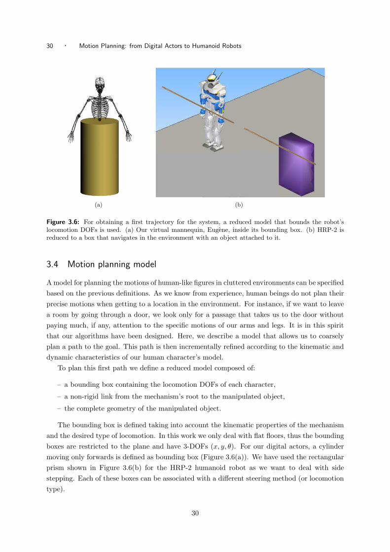
30 · Motion Planning: from Digital Actors to Humanoid Robots
(a) (b)
Figure 3.6: For obtaining a first trajectory for the system, a reduced model that bounds the robot’slocomotion DOFs is used. (a) Our virtual mannequin, Eugene, inside its bounding box. (b) HRP-2 isreduced to a box that navigates in the environment with an object attached to it.
3.4 Motion planning model
A model for planning the motions of human-like figures in cluttered environments can be specified
based on the previous definitions. As we know from experience, human beings do not plan their
precise motions when getting to a location in the environment. For instance, if we want to leave
a room by going through a door, we look only for a passage that takes us to the door without
paying much, if any, attention to the specific motions of our arms and legs. It is in this spirit
that our algorithms have been designed. Here, we describe a model that allows us to coarsely
plan a path to the goal. This path is then incrementally refined according to the kinematic and
dynamic characteristics of our human character’s model.
To plan this first path we define a reduced model composed of:
– a bounding box containing the locomotion DOFs of each character,
– a non-rigid link from the mechanism’s root to the manipulated object,
– the complete geometry of the manipulated object.
The bounding box is defined taking into account the kinematic properties of the mechanism
and the desired type of locomotion. In this work we only deal with flat floors, thus the bounding
boxes are restricted to the plane and have 3-DOFs (x, y, θ). For our digital actors, a cylinder
moving only forwards is defined as bounding box (Figure 3.6(a)). We have used the rectangular
prism shown in Figure 3.6(b) for the HRP-2 humanoid robot as we want to deal with side
stepping. Each of these boxes can be associated with a different steering method (or locomotion
type).
30

Humanoid Representation · 31
The non-rigid link between the root of the model and the object to be manipulated is
defined according to the limits of the individual reachable workspace. The object’s geometry is
not bounded by a box, i.e. all the polygons that define it are considered from the first planning
problem. Its configuration in space is specified with 6-DOFs, unless kinematic constraints are
imposed on it.
For a given motion planning problem, the system is formed by a bounding box for each of
the cooperating character and a non-rigid link from each character’s root, to the manipulated
object.
3.5 Conclusion
In this chapter we have presented the elements to model the problem of trajectory generation
for human-like figures that we try to solve in this work.
In this work we have integrated the three presented principles into a motion planning
algorithm that deals with the generation of human-like, collision-free motions for mechanisms
that walk while manipulating an object.
The constructed system takes into account the geometry and kinematics of the problem,
but it does not consider its dynamics. The mechanisms here studied have complex dynamic
mechanisms and if they are neglected when planning their motions would produce non-desired
results. Efficient motion controllers that simulate the dynamics of human-like mechanisms have
already been developed. In this work we propose a decoupled approach that uses some of this
controllers to introduce the dynamical effects on the motions and then geometrically compensates
these effects to obtain collision-free motions. The method consists on three steps:
1. Plan collision-free motions for the reduced model of the system, considering only for its
kinematic and geometric constraints.
2. Generate the behaviors that make the humanoids follow the specified trajectory.
3. Refine the trajectory to compensate for dynamic effects in collision-free motions.
In the next chapters we develop this approach considering three types of mechanisms: a
human-like digital actor, a large space manipulator and the humanoid robot HRP-2.
31

32 · Motion Planning: from Digital Actors to Humanoid Robots
32

“El simulacro alzo los sonolientos parpados y vio formas y colores que
no entendio, perdidos en rumores y ensayo temerosos movimientos.
Gradualmente se vio (como nosotros) aprisionado en esta red sonora
de Antes, Despues, Ayer, Mientras, Ahora, Derecha, Izquierda, Yo, Tu,
Aquellos, Otros.” 1
Jorge Luis Borges – El Golem
4Digital Actors: Eugene & Co.
Over the last few decades, many attempts to animate the human figure have been made [Parent
2002; Magnenat-Thalmann and Thalmann 1996], each of them attaining a certain degree of
autonomy, interactivity or user-controllability.
As seen in Chapter 3, the human figure has been frequently represented in Computer
Animation in the same way articulated mechanisms are represented in robotics [Badler et al.
1993]. A computer animated sequence can be described, just like a motion in robotics, as an
evolution of state variables (joint angles) over time. However, the techniques developed in both
areas have aimed for different results. In computer animation, the interest has traditionally been
the generation of realistic-looking motions, while in robotics the concern has been to automate
the generation of feasible motion regardless of its appearance.
In recent years, applications arising in both areas (e.g. ergonomics, interactive video games,
etc.) have motivated researchers to automatically generate human-like plausible motion.
In the work presented in this chapter, we are interested in the development of automatic
strategies that produce trajectories for the navigation of human-like figures in 3-dimensional
cluttered environments. For the sake of interactivity, the motions should be generated as fast as
possible. With this in mind, Pettre [2003] proposed an algorithm that computes eye-believable
motions for a digital actor, which he refers to as Eugene. We have used Pettre’s work as departing
point of the motion planning strategy presented here.
1free tr.“The simulacrum raised its sleepy eyelids and saw forms and colors it did not understand, lost in
whispers and made fearful movements. Gradually it found itself (as ourselves) imprisoned in this reverberatingnet of Before, After, Yesterday, While, Now, Right, Left, I, You, Those, Others.”
33

34 · Motion Planning: from Digital Actors to Humanoid Robots
Our contribution relative to this previous work is to deal with object handling as well as with
cooperation among characters. In this context, several behaviors should be combined within a
single animation sequence: agents should move (walk or roll) while coordinately manipulating
a bulky object. Here, the main challenge is to achieve 3D collision avoidance while preserving
the believability of the agents behaviors.
From an algorithmic perspective, our approach is a centralized one. This means that we
model the global task within a single system that contains all the DOFs of the agents and
their object. The system is built considering the interaction limits imposed by the cooperative
reachable space. The algorithm consists in performing three steps sequentially:
1. Plan a collision-free trajectory for a reduced model of the system.
2. Animate, in parallel locomotion and manipulation behaviors.
3. Tune the generated trajectory to avoid residual collisions.
In order to build our motion planner, we have chosen the techniques that best provide the
desired characteristics to the resulting animation, which are in our case, believable and automatic
motion, precise manipulation and combined behaviors.
Most of the contents of this chapter have been presented in Esteves et al. [2006]. In the
following sections we make an overview of related work in animation techniques used when
generating motions of digital actors. Then, we describe some of the previous motion planners
available in the literature.
4.1 Animation techniques
Computer animation techniques have been classified by Magnenat-Thalmann and Thalmann
[1991] according to the method used for controlling the movements of the mechanism. This
taxonomy considers the nature of the information given as an input to the controller, giving rise
to three categories: geometric and kinematic, physical and behavioral.
4.1.1 Geometric and kinematic methods
These methods allow motion to be specified independently of the underlying forces that produce
them. Motion can either be defined in terms of geometric coordinates such as joint angles (usually
referred to as articulation variables or avars), or in terms of velocities or accelerations. Among
these methods we find, keyframing, motion capture-based animation or inverse kinematics-based
techniques. Because in our motion planner we consider geometric and kinematic constraints,
the choice of this methods follows naturally. In the next paragraphs we describe them briefly.
Keyframing
This technique comes directly from traditional animation. Here, motion is specified by a set
of “key” states or frames which are automatically interpolated to generate intermediate frames
34

Digital Actors: Eugene & Co. · 35
called inbetweens as described in Burtnyk and Wein [1971]. Different interpolation techniques
might be used depending on the smoothness and timing desired on the resulting motion. The
choice of the interpolation algorithm is crucial to the appearance and eye-believability of the
final motion. In the probabilistic motion planning context, every node in the graph becomes a
keyframe which is interpolated with the appropriate steering method.
Inverse kinematics
As described in Section 3.1.2, this method allows to specify configurations for a portion or for the
entire character’s body2 in terms of the configuration of the extremal linkages or end-effectors.
This means, in our context, that the motion planner can specify a desired configuration for the
character’s hands or feet and the rest of the values for the articulated hierarchy are computed
automatically. In the general case, there is no closed-form solution to the inverse kinematics
problem as there are an infinity of solutions. For this reason, numerical algorithms are frequently
used. These techniques come in handy when trying to adapt motions to satisfy constraints, e.g.
keeping the feet on the ground. Algorithms using this kind of techniques have been described
by Girard and Maciejewski [1985], Tolani et al. [2000], Baerlocher and Boulic [2004], Yamane
and Nakamura [2003b] among many others.
Motion capture
This technique consists in recording or measuring the three-dimensional motions of a physical
object or a human performer (Figure 4.1) in order to apply them to a synthetic model. The
most commonly used technologies for capturing full-body motions are electromagnetic sensors
and optical markers. This techniques have proven to be very useful when trying to generate
human-like plausible motions as the recorded motion contains already the complexity of the
dynamic motion. However, as examples are recorded for specific types of motions and for
specific morphologies, an edition process is, more frequently than not, required. The edition
process has to preserve the realism of the motion as much as possible while allowing to reuse
the data. Motions can be edited when wanting to adapt recorded movements to different
morphologies as in Gleicher [1998] or recently in Kulpa et al. [2005]. Motion capture edition
has led to the development of whole new approaches, the so-called data-driven techniques. The
goal of this methods is to generate new motions from existing recorded examples. A great
variety of techniques have been applied for this. Interpolation methods to combine motions
with different characteristics have been presented for example in Witkin and Popovic [1995],
Unuma et al. [1995] or Rose et al. [1998]. Motions have also been adapted to respect spatio-
temporal constraints adapting to a given path or environment as for instance in Witkin and
Kass [1988], Rose et al. [1996], Popovic and Witkin [1999] or Gleicher [2001b]. Even when using
edition methods, the capacity of generating new motions depends largely on the number and
discriminability of the recorded motions.
2for the rest of this manuscript, we refer to the whole-body configuration of a mechanism as its posture or pose
35

36 · Motion Planning: from Digital Actors to Humanoid Robots
(a) (b)
Figure 4.1: (a) VICON optical motion system in Paris. The performer wears reflective markers on hisclothes (white spots). Position and orientation of the markers are recorded by 24 cameras (red spots)placed on the walls. (b) The recorded marker’s information is processed to reconstruct the motion so itcan then be fitted to a virtual skeleton.
4.1.2 Physical methods
The idea of this approach is to generate realistic (physically feasible and eye-believable) motion
which respects the laws of Newtonian physics. Here, the objects are controlled by applying forces
and torques to the model and computing the system’s evolution in time. Simulated motion is
plausible if the model captures enough physical characteristics that represent the situation.
These kind of methods should be able to handle penetrating impacts and true contacts with
the environment to provide the desired realism to the motions. For this, a good description
of the objects and forces coming from the environment is needed. However, these techniques
are difficult to apply to virtual characters because a large amount of physical data is needed to
find all the forces and their interactions. These algorithms may also consider the behavior of
the simulated muscles, the character’s stability and many other constraints, which makes them
computationally expensive. Recent physically-based techniques are based on works in artificial
intelligence where a controller can be adapted according to the situation. An example of physical
methods used on virtual humans is presented in Hodgins et al. [1995].
4.1.3 Behavioral methods
These kind of approaches are located on a higher level that those described above. Here, the
characters are supposed to be autonomous creatures, capable of determining their own actions
and with capabilities that characterize natural life (evolution, perception, learning, emotions,
etc.) These models include for instance, those inspired on theories of natural evolution [Sims
1994] or those which take into account behavioral rules of agents interacting with each other
[Reynolds 1987]. The control inputs for these methods are usually directives indicating a
36

Digital Actors: Eugene & Co. · 37
particular behavior to be performed by the character. These behaviors can be modified with the
character’s own motivations, interpretations and interactions with the environment, as described
by Blumberg and Galyean [1995]. A survey of behavioral methods can be found in Terzopoulos
[1999].
4.2 Motion planners for virtual characters
In the context of probabilistic motion planning, several algorithms that produce collision-free
human-like trajectories have been proposed in the literature. These planners are mainly based
on the use of geometric and kinematic approaches, because the integration of these constraints
in the planning framework is straightforward. These works have mainly focused on generating
trajectories either for locomotion or for manipulation. Our work proposes to deal with both
behaviors in a unified manner.
4.2.1 Motion planning for walking characters
In order to generate plausible human-like motions, techniques based on motion capture have
frequently been used. These techniques have proven to be suitable for real-time motion
generation. As we are dealing with a kind of motion that is repetitive by nature, controllers
based on motion capture are particularly adequate: only a few number of motion examples
suffice to drive the character from one configuration to another. Various motion planners that
exploit motion capture-based techniques have been proposed. Kuffner [1998] presents a two-step
approach that consists in first planning a collision-free path for a cylinder and then following
it by means of a PD controller that uses cyclic motion capture data. In Choi et al. [2003] the
authors deal with rough terrains by planning the character’s footprints and adapting captured
motion data to attain them. In the same lines as the former planner, Pettre et al. [2003] proposed
a three-step motion planner that deals with the 3-dimensionality of the environment by applying
the collision avoidance-based warping method despicted in Section 4.3.3.3.
4.2.2 Motion planning for object manipulation
As far as manipulation and reach planning for virtual characters are concerned, the problem has
been tackled using different approaches. Liu and Badler [2003] plan and synthesize collision-free
reaching motions for 7-DOF arms in real time by using graphics hardware to detect collisions.
Their planning framework reasons directly in the workspace. However, this kind of planning
approach has not proven to be more efficient than the configuration-space planning approaches
as used in Kallmann et al. [2003] and Yamane et al. [2004].
In Kallmann et al. [2003], the authors plan reaching motions for a 22-DOF system (9
DOFs for each arm and 4 additional DOFs to specify the character’s body posture). Inverse
kinematics algorithms are used to specify the initial and final configurations, and a roadmap
is constructed based on the cost computed for each configuration. This approach can manage
obstacles displacements by dynamically updating the roadmap.
37

38 · Motion Planning: from Digital Actors to Humanoid Robots
(a) (b) (c)
Figure 4.2: (a) Windscreen wiper motor assembly. A first collision-free path is computed for the partalone. (b) The character follows the path using an inverse kinematics operator to grasp the object. (c)A radiator assembly with two-hand grasping.
When dealing with object handling, the object is usually specified as the goal to be reached
by the end-effector using an inverse kinematics algorithm. The large number of DOFs present
on a virtual character makes it necessary for these algorithms to consider the redundancy of the
system. If the object in question is grabbed with only one arm, the typical approach is to specify
the configuration of the object and then to use an analytical algorithm of inverse kinematics
for a 7-DOF arm as that described in Tolani et al. [2000]. When the problem involves seizing
a rigid object with two hands as in Koga et al. [1994] and Yamane et al. [2004], a trajectory
is first found for the object to be manipulated or grasped and then the loop is closed between
the arms and the object to follow the computed trajectory. The former approach considers for
manipulation planning, allowing regrasping, the latter uses a set of captured motion data in
order to adapt the results of an inverse kinematics algorithm towards natural postures.
In our work, we deal with manipulation similarly, the configuration of the object is
automatically specified by the motion planning algorithm and imposed in the form of
independent tasks for each hand. Our contribution is to address the grasping task (the closed
kinematic chain) at the planning level itself. Our manipulation planning algorithm has been
extended to consider highly constrained spaces in the context of assembly of mechanical parts
giving rise to two strategies, presented in Laumond et al. [2005]. The first one consists in first
planning an assembly path for the part alone; then an inverse kinematics operator computes
the motions the character has to perform to execute the assembly path as shown in Figure 4.2.
The second strategy is used when the first one fails. It consists in searching ,with a diffusion
algorithm, the configuration space of both, the character and the grasped part together. In that
case, the system appears as a high-dimensional one, making the planning more challenging, but
allowing to address very constrained environments.
38

Digital Actors: Eugene & Co. · 39
4.2.3 Combining behaviors
The problem of combining behaviors of articulated human figures has been frequently tackled in
computer animation by applying behavior-based controllers as in Perlin [1995] or in Brand and
Hertzmann [2000]. Here, motion capture data is labeled as containing one particular behavior
or characteristic (run, walk, scratch head, etc.). A new walking-scratching head sequence can
be generated by interpolating configurations of the original captured data.
Kovar et al. [2002] captures a set of labeled motions examples in a graph. A believable
animation is produced by composing motion captures corresponding to chosen edges and the
transitions between them (nodes). A path can be followed by minimizing the error between the
path in the graph and and the user-sketched one. In Kallmann et al. [2004], a sampling approach
using parameterized motion primitives is used to satisfy a given task. Motion primitives are
chosen by means of a tree in which nodes are valid configurations reachable by more than one
primitive and edges represent the paths between them. Their chosen parameterization allows
the computation of trajectories maintaining constraints, such as balance, along it.
Physically-based solutions are described in Shiller et al. [2001] where a simple motion planner
is presented to combine behaviors (walking, crawling and side-walking) in a sequential manner.
Another approach is presented in Faloutsos et al. [2001] where individual controllers generating
different behaviors are managed by a supervisor controller.
In our work, combination or behaviors is straightforward because of the functional
decomposition of the system’s DOFs. Locomotion behavior is computed for the locomotion
DOFs and manipulation behavior animates the arms.
4.3 Our approach
In order to generate complete motion sequences for one or more virtual characters transporting
a bulky object in cluttered environments, we use three main components:
– a motion planner that handles open and closed kinematic chains,
– motion controllers adapted for virtual human-like characters and virtual robots.
– a three-dimensional collision avoidance editing strategy.
Many existing techniques can be used to cover these requirements. In the paragraphs that
follow, we describe those that we experienced as the best adapted to our problem.
4.3.1 The motion planner
As it was described in Chapter 2, the aim of a motion planner is to obtain a representation
of the topology of Cfree in a roadmap. This structure is then used to find a collision-free path
from an initial configuration or state, to a final one, both specified by the user. We have chosen
to use the Visibility PRM algorithm described in Section 2.2.1. The fact that this method is
based on the construction of a roadmap makes it is well-adapted to multiple-query problems,
39

40 · Motion Planning: from Digital Actors to Humanoid Robots
(a) (b)
Figure 4.3: (a) The closed kinematic chain formed when grasping an object with two hands isdecomposed in active (the object and the clavicles) and passive (the arms) parts in order to plan itsmotion. (b) An approximation of the space that can be reached by a character holding an object withtwo hands.
useful in our applications. Another property of the V-PRM algorithm is that as it produces
a compact roadmap, qinit and qgoal are connected with a reduced set of edges. In addition to
this planner, we use the RLG algorithm presented in Section 2.3.1 to include closed kinematic
chains. As explained before, the closed chain is divided in active and passive parts (Figure
4.3). Collision-free configurations are sampled in C and inverse kinematics algorithms are used
to maintain closure constraints.
4.3.2 The behavior controllers
Once a path is found, the appropriate motions to follow it as accurately as possible should be
produced. In the following paragraphs we describe the techniques used to generate such motions
for walking as well as for manipulating with virtual human-like characters.
4.3.2.1 Manipulation control
As seen in Section 4.1.1, kinematics-based techniques allow the motion to be specified
independently of the underlying forces that produced them. In our approach, IK is used
to provide precise control of the manipulation behavior. Several IK algorithms for 7-DOF
anthropomorphic limbs have been developed based on comfort criteria in order to best reproduce
human-arm motions (e.g. Kondo [1994]; Tolani et al. [2000]). We have chosen to use the analytic
IK method presented in Tolani et al. [2000] to specify the configuration of our virtual character’s
arms. Though the arm’s kinematic chain is redundant relative to the reaching task, the algorithm
is analytic, which makes the computation very fast and robust. This can be done due to the
observation that the shoulder’s and wrist’s joint limits restrict the elbow’s valid configurations.
The elbow joint value is thus determined geometrically in function of the arm’s joint limits and
40

Digital Actors: Eugene & Co. · 41
Figure 4.4: From Pettre and Laumond [2006]. Each captured locomotion cycle is represented as a pointin the v−ω space according to their average linear and angular velocity. A new walking cycle is obtainedby from the interpolation of the three closest sources to the control input u(v, ω).
a user-defined swivel angle. Once this value is set, the rest of the arm’s joints can be easily
found. To specify the configuration of virtual robot’s manipulators with 6-DOF, we use the
exact algorithms described by Renaud [2000].
4.3.2.2 Locomotion control
An extensive survey of human locomotion in the context of computer animation is presented in
Multon et al. [1999]. In our work, we have chosen to use the motion capture-based controller
described in Pettre and Laumond [2006]. Here, the problem is modeled in such a way that the
best motion examples to be blended as well as their respective weights are chosen by a simple
geometric computation. The key idea is to represent all the motion examples inside a given
library, as single points lying in a 2-dimensional velocity space (linear and angular velocities)
as shown in Figure 4.4. These points are then structured into a Delaunay triangulation, a
well-known data structure in computational geometry, which allows efficient queries for point
locations and nearest neighbor computations. The control scheme is based on a blending operator
that combines three sources of motion capture. Their respective weights are automatically
computed by solving a simple linear system with three unknown variables. The input parameters
of the locomotion controller are, therefore, the sequence of sampled (vt, ωt), where vt and ωt are
the linear and angular velocities of the virtual characters trajectory. Then, for each pair (vt, ωt)
that represents one locomotion cycle, the three motion capture sources (v1, ω1);(v2, ω2), and
(v3, ω3), with the closest average speeds to the sampled velocities are blended. As a result, a
new locomotion cycle with the desired velocities is computed.
Finally, in order to obtain a continuous animation along the trajectory, the frequency
characteristics of each cycle are computed and cycles are interpolated as described in Pettre
41

42 · Motion Planning: from Digital Actors to Humanoid Robots
(a) (b)
Figure 4.5: Starting and goal configurations of the system for our workout example.
and Laumond [2006]. Other locomotion controllers based on motion capture data, such as the
recently proposed in Suleiman et al. [2006] can also be used without losing the properties of our
algorithm. The main idea in that work is to identify the relationships between the input motion
capture signals and to describe a model based on these relationships. This model takes as input
the trajectory of the waist, which is the output of our motion planning stage.
4.3.3 The algorithm
Our approach relies mainly on three stages: planning, animating and tuning. Several techniques
are suitable for solving each stage. We have adopted some of them in a hierarchical manner to
finally achieve collision-free planning motions for the whole system.
The user-specified inputs for the algorithms are:
– a geometric and kinematic description of the system A
– maximal linear velocity and acceleration P
– number of the desired frame-rate in the animation P
– a motion library containing captured data from different walking sequences MLib
– the maximum number of failures before the algorithm stops ntry
– an initial and a final configuration.
The output is an animated sequence of the combined behaviors A(qi). Algorithm 4.1
summarizes the various steps. In the next paragraphs each stage is described. We use the
workout example of Figure 4.5 to illustrate the algorithm steps.
42
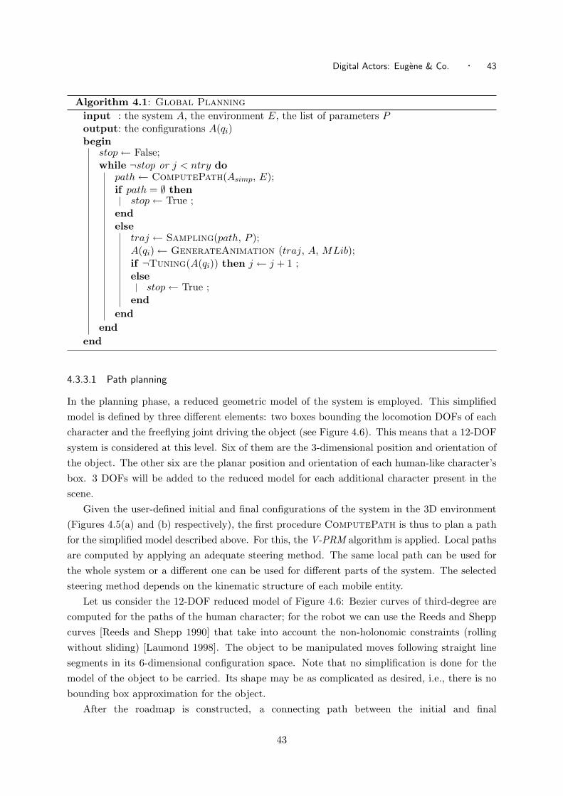
Digital Actors: Eugene & Co. · 43
Algorithm 4.1: Global Planning
input : the system A, the environment E, the list of parameters Poutput: the configurations A(qi)begin
stop← False;while ¬stop or j < ntry do
path← ComputePath(Asimp, E);if path = ∅ then
stop← True ;end
elsetraj ← Sampling(path, P );A(qi)← GenerateAnimation (traj, A, MLib);if ¬Tuning(A(qi)) then j ← j + 1 ;else
stop← True ;end
end
end
end
4.3.3.1 Path planning
In the planning phase, a reduced geometric model of the system is employed. This simplified
model is defined by three different elements: two boxes bounding the locomotion DOFs of each
character and the freeflying joint driving the object (see Figure 4.6). This means that a 12-DOF
system is considered at this level. Six of them are the 3-dimensional position and orientation of
the object. The other six are the planar position and orientation of each human-like character’s
box. 3 DOFs will be added to the reduced model for each additional character present in the
scene.
Given the user-defined initial and final configurations of the system in the 3D environment
(Figures 4.5(a) and (b) respectively), the first procedure ComputePath is thus to plan a path
for the simplified model described above. For this, the V-PRM algorithm is applied. Local paths
are computed by applying an adequate steering method. The same local path can be used for
the whole system or a different one can be used for different parts of the system. The selected
steering method depends on the kinematic structure of each mobile entity.
Let us consider the 12-DOF reduced model of Figure 4.6: Bezier curves of third-degree are
computed for the paths of the human character; for the robot we can use the Reeds and Shepp
curves [Reeds and Shepp 1990] that take into account the non-holonomic constraints (rolling
without sliding) [Laumond 1998]. The object to be manipulated moves following straight line
segments in its 6-dimensional configuration space. Note that no simplification is done for the
model of the object to be carried. Its shape may be as complicated as desired, i.e., there is no
bounding box approximation for the object.
After the roadmap is constructed, a connecting path between the initial and final
43

44 · Motion Planning: from Digital Actors to Humanoid Robots
Figure 4.6: A 12-DOF reduced geometric model of the system is employed in the planning phase. Eachof the bodies will have an associated steering method while planning a path for the system.
configurations is searched. If the path is found, then the function Sampling transform such
path into a trajectory (i.e., a time parametrized path) with user-defined velocity and acceleration
constraints. Even though this is a classic problem of robotics and several techniques can be
used, in our work we use the algorithm proposed by Pettre [2003], which is dedicated to this
application. Here, the velocity and acceleration limits, as well as the desired sampling rate are
specified by the user. Samples are placed along the trajectory while checking these constraints
are verified. The output of this method are a set of samples (xi, yi, θi, vi, ωi) for the system along
the trajectory required as an input for the next stage.
It is important to note that at this level only the bodies attached to the locomotion and to
the object DOFs are ensured to be free of collisions.
Figure 4.7 shows an example in the 3-dimensional environment. Here, the system is composed
by a virtual human character, a mobile manipulator and an object. The barrier in the middle
of the walk path forces the robot to take the left side while the human can still walk on the
right side (Figure 4.7(a)). In Figure 4.7 some of the configurations of the 12-DOF system are
illustrated. There it can be seen how the object is raised while traversing the barrier and
lowered once it finishes. In this case, each of the characters follow the trajectory computed
for their respective bounding cylinders according to their own steering methods. Note that the
object remains within the reachable space between the human character and the robot during
all the animation.
4.3.3.2 Behavior control
At this stage, the trajectory of the 12-DOF simplified model is already planned. The next step
is to synthesize the motions for the complete system involving the locomotion, adaptability,
and grasp DOFs. This is done in the function GenerateAnimation by applying two
different techniques: a locomotion controller to animate locomotion DOFs (pelvis and legs)
44

Digital Actors: Eugene & Co. · 45
(a)
(b)
Figure 4.7: (a) In the planning step a trajectory is found for the 12-DOF system in a 3-dimensionalenvironment. Here, the barrier in the middle of the scene causes the characters to take different paths.(b) Side view of the trajectory performed by the system. At this stage locomotion and manipulationbehaviors are not yet synthesized. The object is slightly raised in order to avoid the barrier.
45
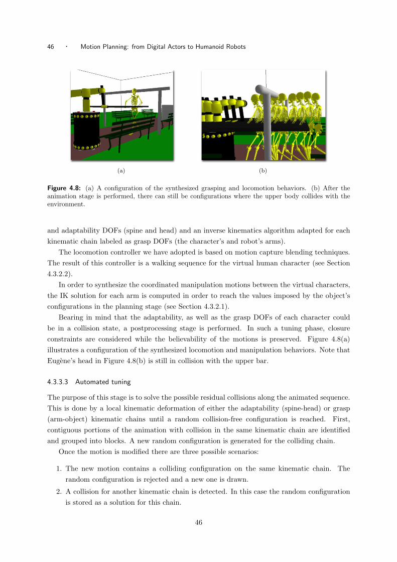
46 · Motion Planning: from Digital Actors to Humanoid Robots
(a) (b)
Figure 4.8: (a) A configuration of the synthesized grasping and locomotion behaviors. (b) After theanimation stage is performed, there can still be configurations where the upper body collides with theenvironment.
and adaptability DOFs (spine and head) and an inverse kinematics algorithm adapted for each
kinematic chain labeled as grasp DOFs (the character’s and robot’s arms).
The locomotion controller we have adopted is based on motion capture blending techniques.
The result of this controller is a walking sequence for the virtual human character (see Section
4.3.2.2).
In order to synthesize the coordinated manipulation motions between the virtual characters,
the IK solution for each arm is computed in order to reach the values imposed by the object’s
configurations in the planning stage (see Section 4.3.2.1).
Bearing in mind that the adaptability, as well as the grasp DOFs of each character could
be in a collision state, a postprocessing stage is performed. In such a tuning phase, closure
constraints are considered while the believability of the motions is preserved. Figure 4.8(a)
illustrates a configuration of the synthesized locomotion and manipulation behaviors. Note that
Eugene’s head in Figure 4.8(b) is still in collision with the upper bar.
4.3.3.3 Automated tuning
The purpose of this stage is to solve the possible residual collisions along the animated sequence.
This is done by a local kinematic deformation of either the adaptability (spine-head) or grasp
(arm-object) kinematic chains until a random collision-free configuration is reached. First,
contiguous portions of the animation with collision in the same kinematic chain are identified
and grouped into blocks. A new random configuration is generated for the colliding chain.
Once the motion is modified there are three possible scenarios:
1. The new motion contains a colliding configuration on the same kinematic chain. The
random configuration is rejected and a new one is drawn.
2. A collision for another kinematic chain is detected. In this case the random configuration
is stored as a solution for this chain.
46

Digital Actors: Eugene & Co. · 47
(a) (b)
(c)
Figure 4.9: From Pettre [2003]. (a) After synthesizing locomotion, a collision is found in the mannequin’shead with the tree branch. (b) The collision is solved by finding a random collision-free configurationwithin the joint limits and warped with the previous animation. (c) The solution is optimized to obtaina smooth motion.
3. The configuration is collision-free. Here, the configuration is kept and a new block is
processed.
The collision-free motion generated randomly is usually not believable because of its high
amplitude. To avoid this, a last step is required to progressively move the character away from
the obstacle. Here we apply a warping procedure considering the two blocks: the original and
the modified one. Such a procedure is typical in computer graphics to modify a sequence of key-
frames when the two blocks have the same number of keyframes. The warping procedure consists
in interpolating only the DOFs of the colliding chain. The parameters of the interpolation are
controlled by the collision checker in order to provide a new configuration for the kinematic
chain which is as close as possible to the original configuration while being free of collisions.
This procedure is computed in function Tuning.
Figure 4.9(a) shows a sequence where Eugene’s head collides with a tree branch. The colliding
configurations are identified and a new, collision-free, solution is found as shown in Figure 4.9(b).
Finally, the motion is optimized to preserve the eye-believability of the final animation as shown
in Figure 4.9(c). In our barrier example the tuning procedure was automatically applied at the
47

48 · Motion Planning: from Digital Actors to Humanoid Robots
(a)
(b)
Figure 4.10: (a) Some configurations of the resulting animation without residual collisions. (b) Thecollision with the upper bar is avoided in the tuning step.
end of the sequence of Figure 4.10(a), where the character slightly lowers its head in order to
avoid the upper bar. This method has proven to work well when small deformations are needed.
Considering the case of collisions involving the grasp DOFs, a local planner based on closed
kinematic chains is used. To deal with multi-loop closure constraints we use the variant of
RLG algorithm for multiple robots. For this, we consider the object DOFs as the active part
of the closed kinematic chain and the grasp DOFs as the passive part. The goal is to make
the active chain reachable by all passive chains simultaneously. This is done by performing a
guided-random sampling of the active chain within the intersection space formed between the
reachable space of each passive chain. The configurations of passive chains are found using
inverse kinematics. This procedure is illustrated in the pizza delivery example in Section 4.4.
4.3.3.4 Failure Recovery
After these three stages, if all configurations are not collision-free, the path generated in the
first planning stage is invalidated. We remove from the roadmap the edge corresponding to the
48

Digital Actors: Eugene & Co. · 49
local path where the tuning step failed. Then a new global search is performed in order to find
a new path.
4.4 Results and discussion
Our algorithm has been implemented within the motion planning platform Move3D [Simeon
et al. 2001]. In the following paragraphs examples of various scenarios and characters are
presented.
4.4.1 Eugenio, “el Mariachi”
In this example, Eugene is asked to take a bottle of Tequila to his guests. The tray with
the bottle and the glasses is expected to keep horizontal during the trajectory. We have thus,
removed the degrees of freedom that allowed the tray to turn. Our living-room environment is
small and contains large objects (e.g. a grand piano, a desk, etc.) The walkways are therefore
narrow and residual collisions are likely to occur.
Figure 4.11(a) shows the execution of a trajectory between the grand piano and the wall.
The paintings hanging on the wall make the passage narrower at the tray level. Note the 3-
dimensionality of the trajectory when the object is raised in order to avoid collision with the tail
of the piano. In the animation stage, the arms follow the object and the locomotion controller
is applied to follow the virtual character’s trajectory. In this example no residual collisions were
found.
In Figure 4.11(b) we consider another situation where the trajectory goes between the piano
and the desk. Here, after performing the planning and animation steps, a residual collision
was found between the left arm and the reading lamp. A valid configuration could be found
by randomly modifying the object position (respecting its constraints) and then making the
arms follow by IK. However, since we know from the planning step that the object is collision-
free, a solution that avoids moving the tray is preferred. For this, we profit from the 7-DOF
arm IK capability of using the redundant DOF (elbow) to remove the collision. If there is no
valid configuration found after within the DOFs range, the standard procedure is applied. In
the example of Figure 4.11(b), a valid configuration was found by slightly swiveling the elbow
towards the character’s body.
4.4.2 Pizza delivery service
In this example, Eugene, the virtual pizza delivery boy has to take a pizza box from one office to
another. Here, we would like the mannequin to keep the boxes horizontal along the trajectory
to prevent the pizzas from losing their toppings. For this, we impose kinematic constraints by
restricting two of the six DOF of the free-flying object. This means that in roll-pitch-yaw angle
representation we have removed the DOF allowing the object to pitch and roll.
Once the initial and final configurations (Figures 4.12(a) and (b)), velocity and acceleration
constraints and the number of frames are specified by the user, the algorithm is applied and
49

50 · Motion Planning: from Digital Actors to Humanoid Robots
(a)
(b)
Figure 4.11: (a) Computed trajectory for a character carrying a tray. Here, Eugenio has to raise thetray without turning around to avoid hitting the piano and dropping the glasses. (b). The characterswivels its elbow to avoid colliding with the reading lamp.
50

Digital Actors: Eugene & Co. · 51
(a) (b) (c)
(d)
Figure 4.12: (a) Initial configuration. (b) Final configuration. (c) Some configurations of the computedtrajectory. (d) The mannequin moves his elbow in order to avoid collision with the bookshelf.
51

52 · Motion Planning: from Digital Actors to Humanoid Robots
Figure 4.13: The characters deal with several obstacles while cooperatively transporting a slab.
the animation generated. In Figure 4.12(c) the resulting trajectory is shown as a sequence of
configurations selected for image clarity.
After the locomotion and grasping behaviors were generated, a residual collision was found
between the mannequin’s arm and the bookshelf at the second office entrance. In this case
a solution was quickly found by modifying the elbow’s configuration as it is shown in Figure
4.12(d). Here, this collision was not likely to be avoided in the original path because the doorways
are narrow and the bookshelf is very near the final configuration.
In these examples only four motion capture examples were used to synthesize locomotion.
These capture examples included two straight lines at different speeds and two 45 degree turns,
both left and right. This lack becomes evident when sharp turns are present in the path. This
effect is apparent when the character turns and his feet slide on the floor. This can be corrected
using more captured sources but it is interesting to note the good performance of the locomotion
controller even with a low number of motion captured examples.
4.4.3 In the factory
In this example Eugene and a robot character have to transport a slab in a typical industrial
environment with plenty of complex obstacles (pipes, drums, beams, ventilation units, etc.).
Figure 4.13 shows some configurations of the resulting animation illustrating the trajectory
followed by the system. As the system approaches the final configuration, the slab is turned as
a result of the planning step in order to avoid the pipes.
In the animation stage the locomotion behavior is animated and inverse kinematics is applied
in order to grab the object in its new configuration. At the beginning of the trajectory the human
mannequin head collides with the balcony. This collision is automatically solved in the tuning
step by bending the spine and head of the mannequin. It should be noted that if the balcony were
lower it would be very difficult, if not impossible, to find a bending collision-free configuration
52

Digital Actors: Eugene & Co. · 53
for the mannequin. This is due to the fact that the tuning stage is only applied to the upper part
of the body and in order to avoid a lower balcony a knee flexion would be required. Once the
obstacle is left behind, the mannequin smoothly regains its posture to continue the cooperative
task until the final configuration is reached.
Figure 4.14 shows a set of frames extracted from the final animation. Here, we can see that
the motion of the system remains plausible after applying the three steps in the algorithm. Note
that the trajectory planned for each of the agents in the scene remains collision-free and their
position close enough to keep holding the slab.
Figure 4.14: Some configurations extracted from the final animation.
4.4.4 Buren’s Columns
This example in our version of the Buren’s Columns involves two virtual mannequins, Eugene
and his cousin, that handle a large plate. Here, we have introduced kinematic constraints on
the plate in order to keep it horizontal. Because of this, a 10-DOF reduced model is considered
in the planning step. Figure 4.15 shows a view of the complexity of the environment and the
system.
Figure 4.15: In our version of Buren’s Columns two virtual characters interact to handle a plate.
Figure 4.16 illustrates some frames from the resulting animation. The virtual mannequins
walk along the computed trajectory carrying their plate. The object configuration is then
53

54 · Motion Planning: from Digital Actors to Humanoid Robots
Figure 4.16: Selected frames of the resulting animation.
modified because of the increasing height of the columns. In the third frame an upper view of
the system shows that the computed trajectory for the plate is collision-free. The mannequins
continue to raise their object until it is safe to put it down. The final two frames show that one
of the agents collides with the bar. This collision is solved in the tuning step by bending the
mannequins spine.
4.4.5 Transporting the Piano
In our last example we present our version of the piano mover’s problem with two mobile
manipulators and a virtual mannequin. Here, we want to transport the grand piano in our
living-room environment.
A collision-free path for the 15-DOF reduced system was found between the desk and the
piano chair. Figure 4.17 illustrates some of the synthesized motions for the mobile manipulators
and the human mannequin. The virtual robots move away from each other to avoid the stool
and then regain their posture.
Figure 4.17: Two mobile manipulators and a virtual mannequin cooperating to transport a piano.
The cooperation among the characters is ensured during the animation. The 3-dimensionality
of the resulting animation is mainly seen in the piano configuration. Figure 4.18 shows sequenced
frames of the planned animation in order to avoid collision between the piano and the desk. In
this example no residual collisions were found.
4.4.6 Computational time
The planner has been tested on a workstation Sun-Blade-100 with a 500MHz UltraSparc-IIe
processor and 512 MB RAM. In Table 4.1 the number of polygons in the different environments as
54

Digital Actors: Eugene & Co. · 55
Figure 4.18: The piano should be raised in order to avoid collision with the desk.
well as the polygons in the system are presented. In the industrial environment we have identified
the polygons that participate in the collision test (i.e., the ones below the mannequin’s head
level). In the rest of the environments, all polygons are considered for collision tests purposes.
Environment System
Office- Complete 148,977 17,239
Factory- Complete 159,698 18,347
- Col.Test 92,787
Buren’s Columns- Complete 44,392 24,837
Living-Room- Mariachi 25,007 18,381- 3 character cooperation 16,210
Table 4.1: Model complexity (Number of polygons).
The required time to compute the examples presented above are given in Tables 4.2, 4.3,
4.4, 4.5 and 4.6 (averaged over 100 runs). Here, the results of the planning step are expressed
considering a pre-computed graph of the environment product of the learning phase. The time
taken to build this roadmap was 3.8 s, 1.69 s, 31.4 s, 15.1 s and 3.2 s for the mariachi, the
office, the factory, the columns and the living-room respectively. The time it takes to compute
such graphs varies with the complexity of the environment and the fact that it is a probabilistic
approach. The tables present only the results of the queries. Two different animations were
generated for each trajectory, the second with twice the number of frames.
Given the significantly higher size and complexity of the industrial environment, it is not
surprising that it took more time to compute a collision-free path than the other examples. Note
that the time it takes to compute the path at the planning stage is independent of the number
of frames in the animation.
In the animation step, the fastest in the algorithm, it is clearly seen that computational time
55

56 · Motion Planning: from Digital Actors to Humanoid Robots
Piano (Fig.4.11(a)) Lamp (Fig.4.11(b))
No. Frames 79 157 41 80StagesI. Planner- Path 2.4 – 2.4 0.5 – 0.5- Trajectory 0.3 – 0.7 0.1 – 0.3II. Animation 0.27 – 0.45 0.1 – 0.1III. Residual Col. 0.0 – 0.0 0.13 – 0.26
Total 2.97 – 3.55 0.83 – 1.16
Table 4.2: Mariachi in Living-Room (time in seconds).
In the Office
No. Frames 308 609StagesI. Planner- Path 0.5 – 0.5- Trajectory 2.0 – 3.8II. Animation- Locomotion 0.8 – 1.6- Manipulation 0.3 – 0.5III. Residual Col. 0.2 – 0.4
Total 3.8 – 6.80
Table 4.3: Office (time in seconds)
In the Factory
No. Frames 268 530StagesI. Planner- Path 6.5 – 6.5- Trajectory 2.1 – 4.5II. Animation- Locomotion 0.8 – 1.6- Manipulation 0.4 – 0.8III. Residual Col. 5.7 – 11.4
Total 15.5 – 24.8
Table 4.4: Factory (time in seconds)
increases proportionally with the number of frames.
The tuning step relies heavily on the complexity of the environment but also on the number
of frames where there is a colliding configuration. Note that in the living-room example the
time it takes to tune the animation is zero because residual collisions were not found.
4.5 Conclusion
In this chapter we presented an approach to plan and synthesize collision free motions for
virtual characters handling a bulky object in a 3-dimensional environment. To accomplish
this coordinated task, a geometric and kinematic decoupling of the system is proposed. This
decomposition enables us to plan collision-free paths for a reduced system, then to animate the
locomotion and grasping behaviors in parallel and to finally clean up the animation from residual
collisions. These three steps are applied consecutively by making use of different techniques such
as motion planning algorithms, locomotion controllers, inverse kinematics techniques and path
planning for closed-kinematic mechanisms.
At this stage, behavior synthesis is based on the functional decomposition of the system’s
56

Digital Actors: Eugene & Co. · 57
Buren’s Columns
No. Frames 204 405StagesI. Planner- Path 0.01 – 0.01- Trajectory 2.8 – 6.1II. Animation- Locomotion 0.6 – 1.1- Manipulation 0.6 – 1.3III. Residual Col. 3.1 – 5.6
Total 7.11 – 14.11
Table 4.5: Columns (time in seconds)
Transporting the Piano
No. Frames 78 151StagesI. Planner- Path 3.3 – 3.3- Trajectory 0.6 – 1.3II. Animation- Locomotion 0.2 – 0.5- Manipulation 0.1 – 0.3III. Residual Col. 0.0 – 0.0
Total 4.2 – 5.4
Table 4.6: Living-Room (time in seconds)
DOFs (locomotion, manipulation, adaptability). The advantage of such a decomposition is that
the complexity of the system is reduced at each stage of the algorithm allowing, for instance,
the use of very fast IK algorithms. This decomposition also simplifies greatly the combination
of behaviors generated independently.
The main limitation of this approach is that the motion planner is not as flexible as it could
be. For instance, the characters cannot bend to pick the object from the floor due to the fact
that the grasping DOFs cannot modify the locomotion DOFs. This problem can be solved by
using approaches that take into account the whole character’s body such as in Yamane et al.
[2004], Baerlocher and Boulic [2004], [Kallmann et al. 2003] but increasing computational cost.
In order to make a more general planner, the consideration of the dynamic constraints is
essential. As it can be seen from the results presented here, and particularly in the Transporting
the Piano example, the generated motions when lifting a heavy object are identical to those
when a lighter object is involved. This puts at stake the believability of the motions obtained
by using a motion capture-based controller. One way to deal with this problem could be by
integrating a dynamic filter as proposed by Yamane and Nakamura [2003a], but this should be
done while preserving as much as possible the current performance of the method.
In the next chapters we present our work towards the integration of dynamics constraints
in the motion planning algorithms. This is done in the context of producing physically feasible
motions for the humanoid robot HRP-2.
57

58 · Motion Planning: from Digital Actors to Humanoid Robots
58
“And now for something completely different . . . ”
Monty Python – Monty Python’s Flying Circus
5Motion planning with dynamic constraints
As we have shown in the previous chapter, considering only the spatial and kinematic constraints
on a motion planning problem is sometimes not enough for generating believable motions. When
the goal is to plan the motions of a real physical system, ignoring the system’s dynamics
is not an option any more. This becomes apparent particularly in applications that involve
significant changes in the dynamic behavior of the mechanism. For instance, when dealing with
manipulation, the produced motion will be significantly different when handling a heavy or a
light object.
The remainder of this work tackles the problem of generating trajectories that are physically
feasible for mechanisms with complex dynamic behaviors. We present two algorithms based on
our 3-stage planning framework and dedicated to two different types of system. Both algorithms
start by generating a path that considers only the spatial and kinematic constraints of the robot.
This path, to which we refer to as base path, is converted into a feasible trajectory by subsequent
refinements until all the system’s constraints are satisfied. The two types of mechanical systems
giving rise to the two algorithms are:
1. Quasi-static systems, those that can move arbitrarily slowly.
2. Dynamic systems, those in which not all the configurations along a trajectory are stable.
For the first type of system we propose a temporal adaptation of the base path. For the
second we define an iterative spatial deformation of the base path. Two example mechanisms
with complex dynamics are used to illustrate our algorithms: a robotic spatial manipulator for
the first kind, and a humanoid robot for the latter.
59

60 · Motion Planning: from Digital Actors to Humanoid Robots
Our main contribution is to provide a practical method to plan physically feasible trajectories
for mechanisms with complex dynamic behaviors and with a large number of degrees of freedom.
This is done while considering 3-dimensional collision avoidance in cluttered environments.
In the next section we describe the two most common approaches to deal with dynamic
constraints in the context of a motion planning problem.
5.1 Available techniques
In Chapter 2 we defined a path planning problem as the one of finding collision-free motions
subject to spatial and kinematic constraints, but disregarding the time of execution. Now,
we define a trajectory planning problem as the one which takes into account, in addition to the
constraints imposed to the system by the environment, the timing needed to execute the motions.
In other words, a complete motion planning problem consists in finding, given a kinematic and
a dynamic model of a mechanism, the control inputs u(t) needed to drive the system from a
given state xinit to a goal state xgoal in the collision-free space.
When dealing with this problem and again, assuming that the environment is completely
known, one of the following two approaches have been usually applied: decoupled or kinodynamic
planning. Both of these approaches, extensively described in the recent textbooks of Choset et al.
[2005] and [LaValle 2006], are briefly presented in the following paragraphs.
5.1.1 Decoupled trajectory planning
As it name suggests, the decoupled approach involves a decomposition of the motion planning
problem in two stages. For each stage a simpleer problem is identified and solved, producing at
the end the desired sequence of controls to execute the trajectory. These two problems are:
1. Compute a collision-free path τ : [0, 1] → Cfree that is only subject to the spatial and
kinematic constraints of the system and its environment. At this point the time of
execution has not yet been specified.
2. Find a time-scaling σ : [0, tf ]→ [0, 1] subject to the actuator constraints. This time-scaling
function assigns a value σ(t) to every time t ∈ [0, tf ] throughout the path. This function
defines the speed of execution.
The timing function, together with the path, provide a feasible trajectory τ(σ(t)) or τ(t),
for short, from which the sequence of controls u(t) to execute it can be deduced.
The path planning problem from the first stage can be automatically computed by means of
the sampling-based methods described in Chapter 2.
The problem of finding an appropriate time-scaling function has been solved using the
techniques proposed by Hollerbach [1983], Shin and McKay [1985] and Bobrow et al. [1985]
among others. In their work, the problem is stated as the one of finding a time-optimal scaling
function σ, subject to the actuator limits, that allows to follow precisely the path provided from
the execution of the first stage.
60

Motion planning with dynamic constraints · 61
Their strategy consists in parameterizing the base path with a single variable, usually the
distance along the path, so as to reduce the optimal control problem to one dimension. In
this way, maximizing the velocity throughout the distance-parameterized path is equivalent to
minimizing the time of execution of the path. The authors proved that the velocity is maximized
by applying saturated acceleration controls to at least one of the actuators. These kind of
saturated controls are called bang-bang controls.
The time-scaling problem can be thus restated as the one of finding the switching points,
expressed as a value of σ(t), between maximum acceleration and decelaration. This problem
is solved by using numerical integration algorithms to maximize the area below a maximum
velocity curve, drawn from the system’s acceleration limits. Once with the switches, the controls
needed to execute the trajectory can be computed using the robot’s dynamic equations.
5.1.2 Kinodynamic motion planning
The term kinodynamic motion planning, introduced in Donald et al. [1993], refers to those
problems which deal, from the beginning, not only with spatial and kinematic constraints but
also with dynamic ones. Here, the search of a trajectory is done directly in the system’s state
space X , which extends the mechanism’s parameters to include its derivatives. It is for this
reason that kinodynamic methods are also called direct trajectory planning approaches.
The crux of these methods is to search, in the state space, for the sequence of controls that
take the mechanism from a current initial state xinit to a desired goal state xgoal.
The initial problem from Donald et al. [1993] stated that these controls should, in addition
to respecting the system’s constraints, minimize the time of execution and maintain the robot
free from collisions throughout the trajectory.
The core of the algorithm is to simulate, from the current system’s state xc, the execution of
all the possible bang-bang controls during a constant time δt. The produced states, reachable
from xc, are linked and stored in a graph only if they are collision-free. The graph construction
stops when the goal can be reached within a certain value of tolerance ǫ. Once the graph is
constructed, a search is performed to obtain the control sequence that optimizes the time it
takes to reach the goal.
The main drawback of this algorithm is that, as the number of possible bang-bang controls
that can be applied from xinit augments, the number of states that need to be explored increases
exponentially.
In order to make the approach practical, LaValle and Kuffner [2001] integrated it within
the framework of probabilistic algorithms, with the RRT formalism. Here, the author’s idea
is to propagate the state of the robot into the future by choosing random bang-bang controls.
From the state xinit, an exploration tree is thus built by applying random control inputs u
over a constant time interval δt. The search is finished when xgoal is approximated with the
predefined accuracy ǫ. A tradeoff has to be found between the accuracy with which the goal is
reached and the time it takes to find a solution. Although the RRT approach does not produce
61

62 · Motion Planning: from Digital Actors to Humanoid Robots
a time-optimal solution it provides, in reasonable time, a solution for real-sized problems.
5.2 Our approach
Our algorithms subscribe to the first type of strategy, the decoupled trajectory planning
approach. Just as the algorithms described above, we are interested in generating collision-
free movements taking into account the kinematic and dynamic constraints of the system. In
order to do this, we use the three-stage planning approach described in Chapter 1 and depicted
in Figure 5.1. These three steps are:
1. Find a path for a reduced model of the system that takes into account the spatial and
kinematic constraints that the problem imposes.
2. Use available controllers to simulate the execution of the specified behaviors. These
controllers assign, throughout the path, a value qi(t) to every articulation of the
mechanism.
3. Refine this trajectory until all the spatial, kinematic and dynamic constraints are satisfied.
In spite of having the same goal as the decoupled methods described above, our statement
of the problem differs. Here, we are not interested in following exactly the path computed in
the first step, but only to use it as a basis for generating feasible collision-free motions. In other
words, we relax the spatial constraints imposed by the initial path, by performing a dynamic
approximation of it.
This approach results in trajectories that solve, practically, the problem of providing collision-
free, physically feasible motions to take a real-sized system from its initial state to a final state.
As we have stated before, the proposed method is an off-line technique and works under the
assumption that the environment is completely known.
We have applied this three-step strategy to both, quasi-static and dynamic mechanisms,
using a different refinement algorithm to meet the system’s dynamic specifications.
The rest of this chapter is devoted to present our method applied to quasi-static mechanisms.
First, we introduce the 6-DOF spatial manipulator which serves to illustrate our strategy. Even
though this mechanism is slightly out of the scope of this work, it has been useful to introduce
the dynamic constraints into our approach. Then, we describe the three-steps applied to this
particular problem and present the temporal reshaping method needed to fulfill the requirements
of the third step. At the end of the section, simulation results are shown. Finally, Section 5.4
concludes this part of our work. The methods presented in Section 5.3 have been previously
published in Belousov et al. [2005].
62

Motion planning with dynamic constraints · 63
Figure 5.1: Our three-step approach consists in (1) finding a kinematic path for the mechanism, (2)generate, with available dynamic controllers the required motions to execute this path, and (3) reshapethe trajectory to eliminate the collisions appeared due to the dynamic behavior of the system.
63

64 · Motion Planning: from Digital Actors to Humanoid Robots
5.3 Quasi-static mechanisms
As we explained at the begining of this chapter, we refer to quasi-static mechanisms to those
which can move arbitrarily slowly. This means that they are strong enough to maintain any
kinematically feasible configuration without losing, for instance, their balance. Among the most
representative examples of this kind of systems are the robotic manipulators. We have thus
chosen a space manipulator with a significant dynamic behavior as a workout mechanism.
5.3.1 Workout example: Buran
Our workout mechanism is the 6-DOF remote manipulator system (RMS) on board of the
Russian space shuttle Buran. This was done in the context of the project of enhancing the
functionalities of the Virtual Robotic Testbed (VRT), developed several years ago in the Robotics
Laboratory of the Keldysh Institute of Applied Mathematics. The VRT is able to simulate, in
real-time, the dynamic behavior of the space manipulator in zero gravity conditions.
We have tackled the task of docking a satellite in the cargo bay of the space shuttle Buran.
For us, the goal here is to provide an automatic strategy to generate collision-free motions in very
constrained spaces. The developed method is applicable to robot manipulators and quasi-static
systems with arbitrary kinematic and dynamic parameters.
5.3.1.1 Description of the physical system
The Buran space shuttle, shown in Figure 5.2 was built mainly with the intention of performing
tasks of maintenance of space objects and return them to earth when needed. The shuttle’s
length and height are 35.4m and 16.5m respectively. In its middle part, it contains a payload
bay with a diameter of 4.6m and a length of 18m. Inside this bay is installed the RMS, which
is used to handle space objects.
The manipulator is 15.5m long when completely extended, has six degrees of freedom and a
grip that allows the handling of heavy loads of up to 30 tons. The RMS can reach, without a
load, a maximum speed of 30cm/s and when fully loaded, a maximum of 10cm/s. The base is
considered fixed as the large difference of inertia makes its movement negligible.
The main difficulty of dealing with this system, as far as motion planning is concerned, is that
the complexity of its dynamic behavior, produces large deviations from any previously planned
kinematic path. This complexity is mainly due to the elasticiy of its joints and mechanical gears
as well as for the huge loads they usually handle.
In the following paragraphs we describe the implementation of the three-step approach.
5.3.2 The kinematic path
A path subject to geometric and kinematic constraints can be found using the techniques
described in Chapter 2. Here, as the number of DOFs is small and a functional decomposition
is not available, we do not use a simplified model of the system to find this path.
64

Motion planning with dynamic constraints · 65
Figure 5.2: The Buran space shuttle has, in its middle part, a payload bay where the 6-DOF, 15.5mlarge RMS is installed (photo taken from http://www.buran-energia.com).
To plan the motions of the RMS, we have adopted the automatic parameter-tuning diffusion
algorithm proposed by Ferre and Laumond [2004]. This algorithm is intended to work precisely
in the highly constrained spaces frequently found in assembly tasks.
The algorithm is iterative: a first path is computed allowing the system to slightly penetrate
the obstacles. Subsequent paths are refined by decreasing the allowed penetration threshold
where needed. This method benefits from several aspects of recent progress in the motion
planning research field. These are, above all (1) the efficient use of the collision detector by
using lazy-approaches [Bohlin and Kavraki 2000; Sanchez and Latombe 2001] and intensive
distance computations and (2) a parameter-free diffusion process [Ferre and Laumond 2004].
This method works in the same spirit as the approach introduced by Barraquand and Ferbach
[1994], where the search is performed by iteratively growing the obstacles that were formerly
shrunked. Here, the growing process is automatically controlled. Moreover, the failures due
to the passages that can be, at some point closed as a result of the growing process, are
automatically solved.
All of the motion planners described in the remaining of this work, have been integrated in
the KineoPathPlannerTMplatform. The output of the kinematic path planner is a finite sequence
of via-points, connected by a local method, in this case linear interpolation in the configuration
space. Figure 5.3 shows the kinematic path solving the task of docking the satellite inside the
cargo bay.
5.3.3 Dynamic motion generation
As it was mentioned earlier, the RMS can be regarded as a fixed-based manipulator, due to the
large inertia of its links relative to its base. However, in contrast to industrial robot arms, its
65

66 · Motion Planning: from Digital Actors to Humanoid Robots
(a) (b)
Figure 5.3: First step of the algorithm. (a) Collision-free path produced with our kinematic planner. (b)Swept volume showing some configurations along the collision-free kinematic path.
dynamic behavior is very complex given the elasticity of its joints and the large mass and inertia
of its links.
To generate the dynamic behavior of the arm, we have used the real-time dynamic simulator
developed at the Keldysh Institute of Applied Mathematics and described in Belousov et al.
[1995].
This simulator relies on an efficient formulation of the dynamic equations and on fast
integration algorithms. The accuracy of the simulation is, an error of 0.7mm in the manipulator’s
absolute position and 0.1deg in its absolute orientation.
Once the dynamic trajectory is simulated, we perform a collision test throught the trajectory.
The large inertia of this mechanism, together with the highly constrained space, makes the
appeareance of new collisions very likely. Figure 5.4 illustrates this fact by showing one of the
several collisions detected after the dynamic execution of the base path.
5.3.4 Temporal reshaping method
The idea of the temporal reshaping algorithm is, as in the decoupled approaches described in
Section 5.1, to find the appropriate sequence of controls that allow the system to reach the goal
state in a collision-free way. Here, the base path is relaxed in a way that the mechanism is not
bounded to track it, but to keep inside a region computed as function of the distance from the
base path to the closest obstacles. This idea is depicted in Figure 5.5.
The number of control inputs needed to generate the desired trajectory depends on the value
of maximal linear vmax and angular velocities ωmax allowed on the robot’s gripper. The number
of control points is thus computed with:
66

Motion planning with dynamic constraints · 67
Figure 5.4: In the second step of our approach, a collision is detected after the simulation of the realdynamic trajectory.
Figure 5.5: Spatial constraints are relaxed from the initial kinematic path. The mechanism is boundedto keep in a region defined as function of the distance to the closest obstacles.
67

68 · Motion Planning: from Digital Actors to Humanoid Robots
N =T
tc,
T = max
(
Lp
vmax
,φp
ωmax
)
. (5.1)
where tc denotes the period of velocity input control, Lp represents the length of the kinematic
path and φp the maximal difference of orientation.
From this parameters, every control input (vi, ωi) along the trajectory can be specified with:
vi =di
dimax
vmax
(
pAi−1pAi
‖pAi−1pAi‖
)
ωi =di
dimax
ωmax η (5.2)
where di is the distance to the closest obstacle from a point pAiin the path, and dimax
=
max(di) its maximum value. η is the vector of rotation between the two gripper orientations
in points pAiand pAi−1
. This choice of vi and ωi allows to accelerate the robot when it is far
enough from the obstacles (i.e. the coefficient di/dimax≈ 1). Likewise, the robot is decelerated
when the clearance di is small (i.e. the coefficient di/dimax< 1).
In this way, we compute, for each sampled point on the trajectory, the value needed to
control the joint velocities. This is done by multiplying the vector r = [viT , ωi
T ]T by the inverse
Jacobian matrix of the manipulator. When these velocities are derived, a PD control law can
be applied to determine the control inputs to the manipulator.
Now, the remaining problem is the one of choosing admissible maximal velocities to maintain
collision-free motion trying to minimize the overall time of execution of the trajectory. For this,
we have used a dichotomy method. We proceed as following: first we try the maximum values
of linear and angular velocities that can be physically achieved by the robot. If these values lead
to collision during the dynamic simulation, we divide them by two, try the new values and so
on.
As we stated before, this algorithm is not intended to follow the exact kinematic trajectory.
Nevertheless, as it is devoted to quasi-static mechanisms, which can move arbitrarily slowly, the
algorithm converges to the initially planned planned as the velocity approaches to zero.
5.3.5 Simulation Results
The resulting dynamic trajectories for the task of docking a satellite inside the Buran cargo bay
are presented in Figure 5.6.
Here, the number of control points necessary to guarantee collision avoidance was 26. The
algorithm provides a feasible trajectory in an extremely tight space. The minimal distances
throughout the path ranged from 2-3 cm up to 18cm for the 15.5m long RMS handling a 4m
long satellite.
68

Motion planning with dynamic constraints · 69
(a)
(b)
Figure 5.6: Swept volume throughout the collision-free dynamic trajectory. The collisions found aftersimulating the dynamic behavior were corrected with the temporal reshaping algorithm.
69

70 · Motion Planning: from Digital Actors to Humanoid Robots
The resulting trajectory is 18.2025m long and the total time to perform the docking operation
resulted in 98.09 s. The average grip’s linear speed was 18.55cm/s. This value exceeds the
maximum speed of the RMS with payload (10cm/s) and its just a little below its maximum
possible speed, equal to 30cm/s.
We note that the further the obstacles are from the manipulator the faster it will move,
until it reaches its maximal speed. For instance, at the beginning of the trajectory the motion
is faster than at the end, were the environment is much more constrained. At the end of the
trajectory, the mechanism is constrained to follow the planned kinematic trajectory to keep in
the collision-free space.
5.4 Conclusion
The method here presented allows a practical and completely automatic solution for the
generation of feasible collision-free motions for quasi-static mechanisms. The computed motions
can be executed faster than what is allowed by traditional trajectory following methods, due to
the relaxation of the spatial constraints of the base path.
We have demostrated the suitability of our approach in a difficult type of servicing task, in
a highly cluttered environment with a clearance smaller than 3cm. Similar results would have
been difficult to obtain using kinodynamic approaches given the complexity of the mechanism
and the intensive dynamic simulations needed in the diffusion process.
70

“El rabı le explicaba el universo: Esto es mi pie; esto el tuyo; esto la
soga y logro, al cabo de anos, que el perverso barriera bien o mal la
sinagoga.” 1
Jorge Luis Borges – El Golem
6Humanoid Robots: HRP-2
During the last decade, research on humanoid robotics has represented one of the most rapidly
developing axes of robotics. The creation of humanoid robots has been motivated by the idea of
having a device capable of operating in environments made by and for humans, well suited for
human scale, strength and ability. By using anthropomorphic design on robots, researchers have
not sought to copy the human form, but instead, they have inspired from the human functions
relative to their applications and environments. These humanoid machines are expected to
perform autonomously most of the functions a person is capable of without suffering human’s
inefficiencies. For instance, we can imagine a humanoid robot carrying objects or driving heavy
machinery in dangerous constructions sites.
One of the most important and frequent tasks a humanoid robot is expected to perform
is manipulation. In this sense, humanoid robots present a higher potential for performing
manipulation tasks in constrained human-made environments due to their anthropomorphic
nature. In is not unusual, in these kind of environments to find obstacles that most non-
anthropomorphic robots are unable to deal with, as for example, stairs.
Recent progress in the hardware and controllers of humanoid robots, has allowed a panoply
of applications ranging from manipulation [Harada et al. 2005; Nishiwaki et al. 2005; Yoshida
et al. 2005] through perception [Michel et al. 2005; Gutmann et al. 2005] to servicing tasks
[Okada et al. 2005; Yokoi et al. 2006], to mention a few. In spite of the impressive display of
motion capabilities, the automatic generation of trajectories for humanoid robot’s tasks, has
not received as much attention. It is in this respect that humanoid robotics can benefit from
motion planning techniques, which have reached a point of maturity that allows them to deal
1free tr.“The rabbi would explain to it the universe: This is my foot, that’s yours, this the rope; and he got,
after years, for the wicked to sweep the synagogue.”
71

72 · Motion Planning: from Digital Actors to Humanoid Robots
Figure 6.1: Humanoid platform HRP2-14 at LAAS-CNRS. In this work we consider the task of carryinga large object in cluttered environments.
with mechanisms with a large number of degrees of freedom and a great variety of constraints.
One of the key issues to fully exploit the available capabilities of humanoid robots, is precisely
in the development of methodologies that enable them to autonomously explore the environment
and execute various dynamic tasks. These methods should generate dynamic and smooth
whole-body motions that satisfy collision-avoidance constraints and at the same time deal with
locomotion and manipulation behaviors.
Throughout this chapter, we describe a strategy for the generation of automatic collision-free
motions that are feasible by a humanoid robot. We deal in particular with the task of carrying
a large object in a cluttered environment (see Figure 6.1)
Despite the similarity of representation with the virtual mechanism considered in Chapter
4, the strategy there described cannot be directly applied to a humanoid robot. Here, the
consideration of the system’s dynamics is fundamental. Humanoids should keep balanced along
the entire trajectory, and this is an unavoidable fact to be considered when designing a motion
planning strategy. Furthermore, an approach as the one described in Section 5.3 is not suitable
because of the nature of the system. i.e. if we stopped the robot at a random configuration
along the execution of the trajectory, it would, most probably fall down.
In the present work, we aim to provide a method for planning humanoid dynamic motions
based on our three-stage approach. We tackle the problem of carrying a long bar in constrained
office-like environments. We consider the environment to be known and the floor to be completely
flat. Here, in addition to the intrinsic dynamics of the system, the bar’s weight and size may
change the behavior of the system in a way that a feasible path carrying a light bar, is no longer
72

Humanoid Robots: HRP-2 · 73
(a) (b)
Figure 6.2: Simulation of the manipulation task we tackle in this work. Assigning a different weight tothe bar leads to a different posture of the humanoid. (a) Light bar, no collision occurs. (b) Heavy bar,the bar collides with the obstacle.
feasible when carrying a heavy one as seen in Figure 6.2. We propose then, a strategy that is
robust to this variations and is able to adapt to the dynamics of the task.
Our method is based on the three-stage approach described since the beginning of this work:
1. A base path is found using a simple model of the system. The configurations extracted
from this global path are applied to the robot’s root and the carried object.
2. Existing dynamic controllers are applied to generate locomotion and manipulation.
3. Iteratively refine the output trajectory in order to satisfy the spatial, kinematic and
dynamic constraints of the application.
The planning is done in a robust manner in order to cope with different physical parameters
of the object and the dynamic effects due to the system and its task.
The rest of this chapter is organized as follows: Section 6.1 outlines the related work on the
subject and states our contribution relative to these works. Then, in Section 6.2 we describe our
three-stage planning approach applied to humanoid robots. Section 6.3 presents the obtained
results in simulation and on the real robot and finally we conclude in Section 6.4.
6.1 Related work and contribution
Humanoid motion planning has become, during the last few years, a hot topic since it faces the
complexity of planning and dynamic control at the same time.
Among the most active groups of research in the area, Kuffner et al. have proposed
various types of humanoid motion planners [Kuffner et al. 2002; Kuffner et al. 2003; Chestnutt
and Kuffner 2004; Stilman and Kuffner 2005] such as balancing, footstep planning and
73

74 · Motion Planning: from Digital Actors to Humanoid Robots
navigating while displacing movable objects. Locomotion planning for humanoid robots that
pass through narrow spaces has been dealt with, by adapting the locomotion mode according
to the environment [Shiller et al. 2001; Kanehiro et al. 2004]. Okada et al. [2004] addressed
motion planning for collision-free whole-body posture control by performing a similar function
decomposition to the one performed in this work, dividing the robot into movable, fixed and free
limbs and then using an RRT planner. The authors have also proposed a task-oriented motion
planning approach in Okada et al. [2004]. Yoshida [2005] proposed a humanoid motion planner
based on multi-level exploitation of the robot’s degrees of freedom.
Sentis and Khatib [2005] developed a hierarchical controller that synthesizes whole-body
motion based on prioritized behavioral primitives including postures and other tasks in a reactive
manner.
As we have said, motion edition or trajectory adaptation of human-like mechanisms is
not exclusive to humanoid robots. In the domain of computer animation, motion editing is
an attractive and rapidly developing area of research. Gleicher [2001a] presents a survey of
constraint-based methods in computer animation of human-like figures, and more specifically
those methods which deal with spatial and temporal constraints at the same time.
With respect to the related work aforementioned, our contribution is to propose a generic
integrated solution addressing the following issues:
– the three, geometric, kinematic and dynamic constraints in the same planning scheme
– complex tasks including simultaneous dynamic locomotion and manipulation.
The main contribution of our approach is thus, to cover both, manipulation and locomotion
tasks within a single framework. While dynamic motions are addressed in Kuffner et al. [2003]
either for locomotion (footstep planning) or for manipulation (with a fixed base) a combination
of both is novel. On the other side, the whole-body dynamical system framework presented
in Sentis and Khatib [2006] does not address a global motion planning method that considers
locomotion.
From a practical viewpoint, the contribution of this work lies in the integration of available
software into a global motion planning approach that goes up to the experimental verification
on a real platform. Inspired from the motion warping editing techniques [Witkin and Popovic
1995] described in computer animation, we propose a spatial reshaping method that produces
smooth motions. The feasibility of the generated collision-free motions has been verified using
the humanoid platform HRP-2.
6.2 Our approach
Our three step approach, restated to human-like figures with dynamic considerations, is depicted
in Figure 6.3(a). This leads to the reshaping strategy illustrated in Figure 6.3(b) which goes as
follows:
74

Humanoid Robots: HRP-2 · 75
(a)
(b)
Figure 6.3: Path reshaping considering a dynamic task (a) Three-step strategy applied to the problemof humanoid robot motion generation. (b) Motion reshaping strategy.
75

76 · Motion Planning: from Digital Actors to Humanoid Robots
1. Given a desired starting and goal configurations for the robot, plan a path for a reduced
model of the system. The composition of the simplified model is the same as explained
in Chapter 3 and used on the digital actor: a bounding box for the locomotion degrees
of freedom and a the 6-DOF carried object. The main difference here, relative to the
first stage in Chapter 4 is that, with the aim of considering whole-body motions, we have
merged the manipulation and adaptability degrees of freedom into a single group, which
we consider since the first kinematic planning stage. The output of this planner, is thus,
the position and orientation in 3-dimensions (x, y, θ) (the robot is considered to move on
the plane) of the robot’s waist, together with the vector qu providing the values of the
upper body joints, and the 6-DOFs qo specifying the object’s configuration.
2. Generate, with available controllers, the dynamic motion that approximates the given
path. For this stage we rely a dynamic pattern generator which takes as input the vectors
generated on the first stage, as well as other locomotion parameters such as the step length
and speed of execution. The output of this second stage is a dynamically-stable walking
pattern together with all the body joint angles q with a 6-DOF configuration of the robot
in the environment.
3. The dynamic motion is checked for collisions. If collisions, or distance values below a given
threshold are detected, a spatial reshaping method is applied by the kinematic planner.
This modification is applied partially or entirely to the trajectory according to the detected
collisions. This refining process is repeated until all the spatial, kinematic and dynamic
constraints are satisfied. If no solution is found after a given iteration limit, the algorithm
returns to the first stage and another base path is found.
The proposed planning strategy is characterized by collision-free humanoid motion considering
not only dynamic locomotion, but also the dynamics of the executed task. This is, if the task’s
physical parameters change (e.g. the bar might be lighter or heavier), the planner adapts to the
new conditions. In addition, the planner guarantees a safe margin from the carried object and
the humanoid robot to the obstacles in a way that the generated path is robust enough against
execution errors.
In the following sections we precise each of the steps of the approach. This approach has
been previously published in Yoshida et al. [2005] and Yoshida et al. [2006].
6.2.1 Kinematic path planner
This section addresses the algorithmic issues concerning motion planning for a simplified system
with spatial (3-dimensional collision avoidance) and kinematic (object manipulation) constraints.
The goal of this stage is to provide collision-free admissible paths allowing a humanoid robot to
perform simultaneously locomotion and manipulation behaviors. These paths should be robust
enough as to guarantee their dynamic execution.
Two global kinematic planners are used in this work. These planners benefit from the
respective advantages of both, sampling and diffusion probabilistic approaches. The first one, is
76
Humanoid Robots: HRP-2 · 77
a multiple-query method that plans a global path in the reduced system’s configuration space
while the second is devoted to spatial path reshaping. In the following paragraphs we describe
the first global planner.
As we have said, the goal of this step is to produce a plan that guarantees to be collision-free
for both, the robot and the object. For this, we use the functional decomposition of the robot’s
body already experienced in Chapter 4. At this level, the robot is modeled as a geometric
parallelepiped bounding box. Only these box and the complete geometry of the object to be
manipulated are considered at this point. The configuration space to be searched is therefore
9-dimensional, (3 DOFs for the box and 6 DOFs for the object). To explore these space, we
use the Visibility PRM method described in Chapter 2. Here, we consider the shape of the
bounding box as an additional kinematic constraint for the humanoid’s locomotion behavior.
As we want the robot walking in as “naturally” as possible (we do not want it to walk sideways
unless necessary), we consider two different steering methods to build the roadmap. The first
one is based on the use of the Dubin’s curves (sequence of straight lines and arcs of circle)
[Dubins 1957] that enables to consider the non-holonomic nature of these forward motions (the
humanoid motion should be tangent to the path). The second steering method corresponds
to a holonomic mode where the humanoid is considered an omnidirectional system. Here, the
steering method consists in computing straight line segments between two configurations of the
robot (two nodes).
The roadmap is thus built in two steps: first, only the Dubin’s curves are used. After this,
the current roadmap is enriched to improve the covering and connectivity by using the holonomic
mode. In such a way, nonholonomic natural paths are privileged.
As the object is concerned, the configurations are randomly chosen under two constraints:
– collision-free configurations.
– reachable configurations and closure constraints.
For this, the manipulation model described in our modeling of the system and the RLG
algorithm described in Chapter 2 are used. At this stage, the method provides a path in a
9-dimensional configuration space. The complementary upper body configurations of the arms
are computed, either with analytic inverse kinematics algorithms, as for the virtual actor, or
with numerical inverse kinematic techniques that handle multiple priorities as in Yamane and
Nakamura [2003b] or Baerlocher and Boulic [2004]. Aiming at a whole-body generation strategy,
in this work we explore the latter strategy.
6.2.2 Dynamic pattern generator
The walking pattern generator is based on the preview control of the zero moment point (ZMP
[Vukobratovic 1990]) proposed by Kajita et al. [2002]. Based on preview control of the ZMP
position and a linear pendulum model, this method enables to generate biped walking motion
for arbitrary foot placements. More precisely, the pattern generator takes as input a sequence
77

78 · Motion Planning: from Digital Actors to Humanoid Robots
(a) (b)
Figure 6.4: Two kinematic paths computed for the simplified model of the system and with two differentclearance parameters. The difference can be seen in the configurations near the cabinet.
of footsteps, the respective configuration of the robot’s root (located on the pelvis) and tuning
parameters such as footstep length, double/single support ratio, etc.
The result of this operations is a vector q of joint values defining the entire humanoids
posture and the robot’s configuration in the workspace, sampled every 5ms. If a upper-body
configuration is given as input to the pattern generator, the results includes the computation of
its dynamics and modifies the motion to satisfy dynamic constraints.
Although not used at this point in our approach, the walking pattern generator is able to
provide stairs climbing motion.
After executing the pattern generator, we test the trajectory for collisions. If collisions are
detected, a smooth spatial reshaping strategy is required to satisfy the spatial constraints. Once
the collisions withdrawn, the dynamic validity of the reshaped trajectory is verified.
6.2.3 Smooth spatial reshaping
As stated in the previous sections, a collision-free path issued from the motion planning stage,
will not always result in a collision-free dynamic trajectory. For instance, in the example of
Figure 6.5 unexpected collisions arose due to the influence of the dynamics of the task in the
execution of the path. To solve this, an iterative procedure is performed by applying a local
deformation of the dynamic trajectory. If the user-specified number of maximum iterations is
reached and the collision has not been solved, the original path is invalidated and a new one is
found.
The reshaping procedure is illustrated in Figure 6.6 and detailed in the next paragraphs.
78

Humanoid Robots: HRP-2 · 79
(a) (b)
Figure 6.5: The path resulting from the kinematic motion planner is approximated with a dynamicwalking pattern generator. (a) The dynamics of the task produces a deformation of the initially plannedmotion. (b) A collision is produced due to the weight of the bar, neglected during the computation ofthe first path.
(a) (b) (c) (d)
Figure 6.6: (a)Collision-free kinematic path. (b) Each configuration of the dynamic trajectory sampledat 5ms is checked for collisions. Colliding portions of the motion are identified. (c) A collision-freeconfiguration for the upper body is found for each of the colliding ones by augmenting the minimumclearance value to the obstacle. (d) The new collision-free motion replaces the colliding one and smoothlyinterpolated with the rest of the trajectory.
79

80 · Motion Planning: from Digital Actors to Humanoid Robots
The dynamic pattern generator’s output is a vector of configurations sampled at each 5ms.
Each configuration provides the robot’s location as well as the robot’s posture during the
motion. Different motion editing techniques that enforce spatial and temporal constraints as
those presented in Gleicher [2001b] could be used as a reshaping strategy. Our reshaping method
is a variation of the one presented in the Tuning step of Chapter 4.
At this point, this method modifies only the upper part of the robot’s body while keeping
the trajectory initially found for the lower part.
Giving the configuration vector as input, each configuration is tested for collision. The
colliding configurations are identified and separated in collision blocks or portions with initial
configuration u1 and final configuration u2 Figure 6.6(b). For this portions of the trajectory, the
value of minimum clearance2 from the obstacle is augmented and configurations are re-checked
for collisions. If collisions are found within the lower part of the robot, the original path is
modified with the new clearance value and dynamic motion regenerated. If collisions are found
within the upper part of the body, the following reshaping procedure is applied:
First, the limits u1 and u2 of the colliding portion with the new clearance value are identified.
Then, a collision-free configuration is found by randomly sampling in the task space (the object’s
configuration) and satisfying the task specification with the upper body. The lower configuration
is kept as is Figure 6.6(c). The upper collision-free configuration is applied to all the colliding
portion of the trajectory.
Even though at this stage there are no more collisions found in the path, velocity and
acceleration discontinuities are generated at the collision-block limits u1 and u2. For this, the
reshaping limits are redefined by finding the time, thus the number of samples needed to attain
this new configuration given a reference speed vref to perform the motion and a standard
euclidean distance computation between two configurations |qu1− qu1−1| in the configuration
space. With this, the number of samples nsbefore and nsafter (seen in Figure 6.6(c)needed to
smoothly deform and regain the newly found configuration are found.
The rest of the reshaping procedure is done in two steps:
1. A time-parameterized B-spline curve of the form of Eq. 6.1 of order k with n+ 1 control
vertices is fitted for each of the degrees of freedom of the object’s freeflying joint using the
computed position-time pairs (Pi, ti), i = 1, ..., j.
P (t) =
n+1∑
i=1
Bi ·Ni,k(t) (6.1)
which expanded and in matrix form becomes Eq. 6.2
P = N ·B (6.2)
with the computed points in the column matrix P , the basis functions evaluated at the
2Value that specifies the zone from the obstacles boundaries where the robot is considered in collision. If theclearance is negative, the robot is allowed to penetrate an obstacle, if it is positive, a safety zone is created aroundthe obstacle.
80

Humanoid Robots: HRP-2 · 81
computed times in N and the unknown control vertices in column matrix B. Finally, the
curves are resampled at each 5ms to obtain a reshaped trajectory for the manipulated
object.
2. The object configurations are given as input to a generalized inverse kinematics algorithm
to satisfy the smooth manipulation task. This procedure is explained in the following
paragraphs.
6.2.3.1 Half-body collision avoidance
The result of the previous stage is the reshaped motion for the object specifying the task
synchronized with the lower body motion obtained from the previous iteration. The last step is
performed to satisfy the constraints imposed by the task as well as the continuity of the upper
body movements along the new reshaped trajectory. This is done using a generalized inverse
kinematics solver.
We work under the assumption that the displacement achieved in the 5ms between a sample
and the next is small enough to relate the robot’s posture variation qi to the change of the
configuration ri of the link i linearly by the use of the Jacobian matrix Ji.
ri = Jiqi (6.3)
As we are dealing with a mechanism which is highly redundant with respect to the number
of DOFs constrained by the task, we use Equation 6.4 to solve the IK problem for one task (one
hand grasping the bar):
q1 = J#1 ri + (In − J
#1 J1)y1 (6.4)
where J#1 is the pseudo-inverse of the Jacobian matrix, In is the n-dimensional identity
matrix and y1 is an arbitrary optimization vector.
Our IK solver considers two geometric tasks, one for grasping the bar with each hand. In
this case, we solve the second task in the null space of the first task [Nakamura 1991], i.e. The
second task does not modify the first one. This is done when applying Equation 6.5 to the upper
part of the humanoid’s body.
q2 = q1 + J#2 (r2 − J2q1) + (In − J
#1 J1)(In − J
#2J2)y2 (6.5)
with
J2 ≡ J2(In − J#1 J1)
and where y2 is an arbitrary optimization vector. The reference velocity vref is taken into
account as in Yamane and Nakamura [2003b]. Joint limits and more priority levels can be
treated as in the iterative algorithm proposed in Baerlocher and Boulic [2004].
81

82 · Motion Planning: from Digital Actors to Humanoid Robots
(a) (b)
Figure 6.7: The dynamic trajectory is reshaped so as to avoid new collisions. The movement of thehandled object drives the arms of the humanoid robot.
Figure 6.7 shows the result of applying two iterations of the reshaping procedure. In the first
step, the weight of the bar led to the appearance of a collision between the robot’s waist and
the cabinet beside it. The trajectory was reshaped by centering the robot’s body in the narrow
passage, which produced a second collision, this time with the bar. The reshaping procedure
was applied once more leading to the images seen in Figure 6.7(a) and (b).
6.3 Simulation and experimental results
We have conducted simulations and experiments of the proposed humanoid motion planner using
the motion planner from KineoTM, the simulator OpenHRPTM[Kanehiro et al. 2001] and the
hardware humanoid platform HRP-2 [Kaneko et al. 2004] shown in Figure 6.1.
HRP-2 has 30 degrees of freedom, a height of 1.54m and weights 58kg. This robot has
two chest joints for pitch and yaw rotation which extends its motion capabilities which allow
it to even lie down on the floor and stand up. It can carry a load of up to 2kg at each hand.
We present, in this section the example of carrying a 2m bar (with 2.4 cm of diameter) in
two different human-scale office-like environments. The weight of the bar is 0.5kg. We set the
reference velocity vref to be 30cm/s for the bar’s linear and 30deg angular velocities.
6.3.1 Simulation results
A 3-dimensional collision-free trajectory for the humanoid robot has been automatically
computed with the proposed planning method. In this simulation the task of the humanoid
robot is to carry a bar from a initial configuration to a goal configuration in the environment.
Figure 6.8 shows the top view of the environment with the initial and goal configurations shown.
The figure also shows, in dotted lines the path computed for the humanoid’s root. This path
goes through the narrow passage where two high poles make the motion of the bar difficult.
82

Humanoid Robots: HRP-2 · 83
Figure 6.8: Top view of the simulation environment. The two high poles make the problem particularlydifficult.
The robot holds the bar at a height of 0.85m at the initial configuration and throughout
the path, the humanoid lifts the bar to avoid collisions with the box on the table whose highest
position is 1.05m.
Snapshots of the simulation are shown in Figure 6.9 where collision avoidance with several
obstacles is reshaped using half-body motions. Note that the humanoid fully exploits the degrees
of freedom on its arms and chest to be able to go through the passage between the poles (Figure
6.9(d) and (e). The robot arm’s joint limits and the grasping configuration do not allow to
rotate the bar to its vertical configuration. In spite of this kinematic constraint, a collision-free
trajectory is found.
As it is shown, a 3-dimensional collision-free whole-body motion for tasks involving
locomotion and manipulation can be automatically planned using the proposed framework.
6.3.2 Experimental results
6.3.2.1 Bar-carrying example
We have conducted an experiment of the same bar-carrying task in an environment with less
obstacles. The configuration of the arms near the poles was near to reaching the joint limits,
making the trajectory not suitable to implement it on the robot. A similar environment, without
the poles was considered in our experiments. Shortly after start walking, the robot lifts the bar
to move away from the box lying on the table. Figure 6.10 show some of the shots taken during
the motion.
83

84 · Motion Planning: from Digital Actors to Humanoid Robots
(a) Initial configuration (b) Avoiding a lamp
(c) Lifting the bar to avoid a box (d) The left pole is avoided
(e) The bar is horizontally translated to avoid theright pole
(f) Goal configuration
Figure 6.9: Simulation resulting from our 3-dimensional motion planner
84
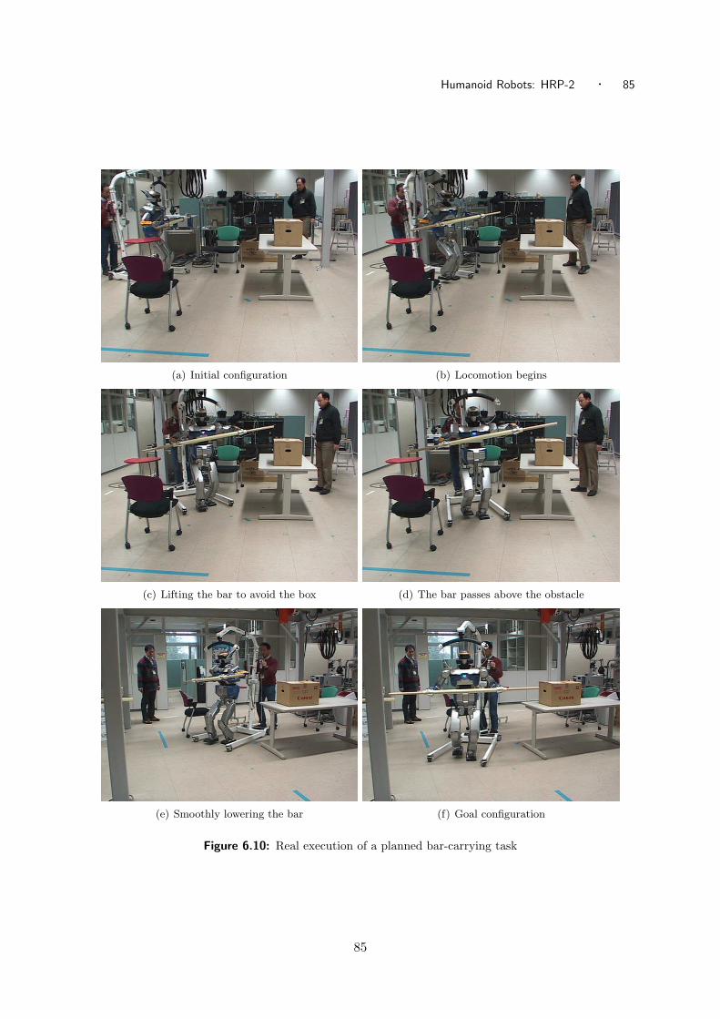
Humanoid Robots: HRP-2 · 85
(a) Initial configuration (b) Locomotion begins
(c) Lifting the bar to avoid the box (d) The bar passes above the obstacle
(e) Smoothly lowering the bar (f) Goal configuration
Figure 6.10: Real execution of a planned bar-carrying task
85

86 · Motion Planning: from Digital Actors to Humanoid Robots
After avoiding the box, the humanoid lowers the bar to the initial height to reach the goal
configuration. The task was successfully achieved by the robotic platform. The validity of the
planned motions is in this way, demonstrated.
6.3.2.2 Barbell example
This example is a variation of the precedent one, with a constrained environment and a more
complicated geometry for the object. The environment is composed of two footlamps and a tall
table. The initial and final configurations are shown in Figure 6.11(a) and (b). The environment
is particularly constrained given that the barbell is larger than the space between the lamps.
At the begining of the motion, the computed trajectory for the barbells make the robot
move to the left (Figures 6.11(c) and 6.12(a)). Here the motion of the upper part of the robot is
computed using a generalized inverse kinematics algorithm with two tasks (left hand to barbell
and right hand to barbell) the chest is moved consequently to complete both tasks.
Without considering the reachable space of the robot, this trajectory would have been
extremely difficult to compute, given that they are few possibilities for the barbell to go thought
the gap between the lamps where the robot is able to grasp it given its joint limits.
This example also shows that the complete geometry of the object has been considered in
the collision-detection and path planning procedure and no bounding box has been used (see
Figures 6.11(e)-(g)) where the dumbell almost circles one of the lamps.
At the end of the motion (Figure 6.11(h)), the tall table is avoided. The complete trajectory
execution time is around 28 sec. The simulation has been done with KineoWorks and OpenHRP
dynamic simulator. Figure 6.12 shows the real execution of the robotic platform HRP-2 14 at
LAAS-CNRS.
6.4 Conclusion
This chapter presented a smooth collision avoidance method for dynamic motion of humanoid
robots. Our three-stage planning method is applied to generate 3-dimensional stable motion for
the humanoid robotic platform HRP-2. This implementation results from the integration of a
geometric and kinematic motion planner with a dynamic pattern generator. Smooth reshaping
of the trajectory was done by applying motion editing methods and cubic interpolation. If the
generated dynamic motion produce collisions, these are subsequently avoided using an iterative
reshaping algorithm.
Future improvements include a refinement of the algorithm to allow more reactive implementation.
The computational time is still in the order of a few minutes in total for planning and dynamic
motion generation. This issue is being currently addressed by making heavy software integration
of the dynamic pattern generator and the kinematic planners.
86

Humanoid Robots: HRP-2 · 87
(a) (b)
(c) (d) (e)
(f) (g) (h)
Figure 6.11: Dumbell experiment simulation (KineoWorks and OpenHRP)
87

88 · Motion Planning: from Digital Actors to Humanoid Robots
(a) (b) (c)
(d) (e) (f)
(g) (h) (i)
Figure 6.12: Real execution on HRP-2 14 platform at LAAS-CNRS.
88

“Part of the inhumanity of the computer is that, once it is competently
programmed and working smoothly, it is completely honest”
Isaac Asimov
7Conclusion: from functional decomposition to
whole-body motion
In this document we have presented a three-stage strategy to plan the motions of human-like
figures in cluttered environments. We have tackled in particular the problem of having an
anthropomorphic mechanism carry a bulky object, alone or in cooperation with others, while
walking around obstacles. We have applied this strategy on virtual and real mechanisms in order
to obtain collision-free trajectories that are realistic relative to the restrictions imposed on the
problem.
We have stated our three-stage strategy as follows:
1. Find a global path that takes the mechanism from a given initial state to a desired goal
state in the 3-dimensional environment.
2. Generate behaviors of locomotion and manipulation that allow the mechanism to
coarsely follow the defined path.
3. Locally refine the trajectory until all the constraints are satisfied.
Our approach relies on a functional decomposition of the mechanism’s limbs which allow
us to produce, at each stage, an appropriate model able to deal with the constraints treated at
that stage. In our walking-while-manipulating problem we have divided the mechanism in three
functional groups: the legs for locomotion, the arms for manipulation and the spine and head
for posture adaptability.
During the first stage a simplified model of the system is proposed in order to obtain a
coarse path for the human-like mechanism and the handled object. This model consists of a
89

90 · Motion Planning: from Digital Actors to Humanoid Robots
volume which bounds the locomotion degrees of freedom and the complete geometry of the
object to be carried. The constraints considered at this stage are:
– collision avoidance for the lower limbs of the mechanism and for the object.
– steering capabilities of the system,
– closure of the kinematic chains that ensure two-hand manipulation and character’s
cooperation.
A path for this simplified model is computed by means of the general probabilistic motion
planning techniques that are able to deal with the above constraints. The advantage of such a
path is that it can be used as a basis for several further adaptations, leaving a certain freedom
on the generation of local behaviors. This by contrast with a footstep planning approach (e.g.
Kuffner et al. [2002] or Choi et al. [2003]), were the step lengths and configurations cannot be
modified without re-planning. However, the fact of planning the motions with a volume moving
in the plane does not allow the consideration of rough terrains, which present no significant
problems when using a footstep planning approach.
The second stage deals with the generation of specific behaviors, in our case locomotion and
manipulation. Here, a wide variety of controllers can be used as long as their input corresponds
to the position or velocity outputs of the global planning stage and as output a value for each
of the degrees of freedom involved in the task. Because of this modular design, our approach
can be seen as a testbed for controllers. In fact, a substantial portion of our collaborative work
is based on using our system in this fashion. Further experiments should be done to determine
the influence of the chosen controller on the overall approach.
The third and last stage is devoted to the avoidance of the collisions generated by the
introduction of the upper part of the body as well as the dynamic constraints. We describe
tuning techniques that incrementally include constraints, starting with spatial and kinematic up
to dynamic considerations. First we have described a tuning strategy that does not jeopardize
the eye-believability of the motions of a virtual character. We have then identified two groups of
mechanisms which we treat differently as far as trajectory reshaping is concerned. For the first
group, the quasi-static mechanisms, we have proposed a time-reshaping strategy which produces
a feasible trajectory by defining its velocity of execution relative to the spatial constraints. For
the second, which we refer to as dynamic mechanisms, we have described an iterative spatial-
reshaping method.
In this work we have tested our strategy by performing experiments on three different
mechanisms: a 53-DOF virtual character, a 6-DOF spatial manipulator and a 30-DOF humanoid
robot. By these means we have obtained eye-believable or feasible trajectories in different
environments with complex geometry and for problems with different constraints. However,
we have identified several limitations in our approach, which has led us to ideas for future
90

Conclusion: from functional decomposition to whole-body motion · 91
developments.
In this research we have worked under the assumption that the tasks the system is to
perform are independent enough from each other as to allow a decomposition of the human-like
figure according to its functions. The nature of our tasks (locomotion and manipulation) makes
this decomposition particularly evident. Nevertheless, if different tasks were to be considered,
independent functionalities might not be easily differentiated. Furthermore, even with the tasks
here considered, a functional decomposition can confine the mechanisms to a limited set of
motions where the behaviors remain independent.
Current research in the group tries to overcome this limitation by considering the entire body
in the generation of behaviors, taking full advantage of the mechanism’s redundancy. We have
presented the first results of this approach in Yoshida et al. [2006]. The task-based method here
proposed is able to generate whole-body motions by augmenting a walking-pattern generator
with generalized inverse kinematics techniques. This approach measures the feasibility of a
task from the current standing point of the humanoid robot . When the goal is declared as
unreachable, a stepping behavior is generated as a result of a simple geometric deformation of
robot’s support polygon. The validity of this approach has already been tested on a humanoid
robot in the context of reaching motions.
We can think of two ways of connecting this work with a global planning strategy. The
first one, following the same lines as proposed in this thesis, by decoupling the planning of the
trajectory into the generation of a global path and then the local behaviors to approximate it.
In other words, the generated whole-body local behavior would merge the last two of our three-
stage approach. A second way is to consider the whole-body local motions as the steering method
in a probabilistic planning scheme. The latter strategy being an integrative approach were the
motion generation is done in a single stage. In our opinion, both of these approaches are worth
exploring as a future work in order to compare their performance and overall computational time.
Finally, one of the guiding principles of our work is the relaxation of the spatial constraints
imposed by the global path when generating local behaviors. This means that we track, instead
of a path, a path region were the robot is allowed to move and constrained to stay. Future lines
of research involve the formal identification of the limits and geometry of this region considering
not only the kinematics but also the dynamics of the mechanism.
91

References
Badler, N. I., Phillips, C. B., and Webber, B. L. 1993. Simulating Humans: Computer
Graphics, Animation and Control. Oxford University Press, Oxford, UK.
Baerlocher, P. and Boulic, R. 2004. An inverse kinematics architecture enforcing an
arbitrary number of strict priority levels. Visual Computer 20, 6, 402–417.
Balkcom, D. J. and Mason, M. T. 2002. Time optimal trajectories for bounded velocity
differential drive vehicles. International Journal of Robotics Research 21, 3, 199–217.
Barraquand, J. and Ferbach, P. 1994. A penalty function method for constrained motion
planning. In Proceedings of the IEEE International Conference on Robotics and Automation.
IEEE Computer Society, San Diego, CA, USA, 1235–1242.
Belousov, I., Esteves, C., Laumond, J.-P., and Ferre, E. 2005. Motion planning for large
manipulators with complicated dynamics. In Proceedings of the IEEE/RSJ International
Conference on Intelligent Robots and Systems. IEEE Computer Society, Alberta, Canada,
3713–3719.
Belousov, I., Kartashev, V., and Okhotsimsky, D. 1995. Real time simulation of space
robots on the virtual robotic test-bed. In Proceedings of the 7th International Conference on
Advanced Robotics. St Feliu Guixols, Spain, 195–200.
Blumberg, B. M. and Galyean, T. A. 1995. Multi-level direction of autonomous creatures
for real-time virtual environments. In SIGGRAPH’ 95: Proceedings of the 22nd annual
conference on Computer graphics and interactive techniques. ACM Press, Los Angeles, CA,
USA, 47–54.
Bobrow, J. E., Dubowsky, S., and Gibson, J. S. 1985. Time-optimal control of robotic
manipulators along specified paths. International Journal of Robotics Research 4, 3, 3–17.
Bohlin, R. and Kavraki, L. 2000. Path planning using lazy PRM. In Proceedings of the
IEEE International Conference on Robotics and Automation. IEEE Computer Society, San
Francisco, CA, USA, 521–528.
Brand, M. and Hertzmann, A. 2000. Style machines. In SIGGRAPH’00: Proceedings of the
27th annual conference on Computer Graphics and Interactive Techniques. ACM Press, New
Orleans, LA, USA, 183–192.
Burtnyk, N. and Wein, M. 1971. Computer generated key frame animation. Journal of the
Society of Motion Picture and Television Engineers 8, 3, 149–153.
Canny, J. F. 1988. The complexity of robot motion planning. MIT Press, Cambridge, MA,
USA.
Chadwick, J. E., Haumann, D. R., and Parent, R. E. 1989. Layered construction for
92

Conclusion: from functional decomposition to whole-body motion · 93
deformable animated characters. In SIGGRAPH’89: Proceedings of the 16th annual conference
on Computer Graphics and Interactive Techniques. ACM Press, Boston, MA, USA, 243–252.
Chestnutt, J. and Kuffner, J. J. 2004. A tiered planning strategy for biped navigation.
In Proceedings of the IEEE International Conference on Humanoid Robotics. World Scientific
Publishing Company, Los Angeles, CA, USA.
Choi, M. G., Lee, J., and Shin, S. Y. 2003. Planning biped locomotion using motion capture
data and probabilistic roadmaps. ACM Transactions on Graphics (TOG) 22, 2, 182–203.
Choset, H., Lynch, K. M., Hutchinson, S., Kantor, G., Burgard, W., Kavraki, L.,
and Thrun, S. 2005. Principles of Robot Motion: Theory, Algorithms and Implementations.
The MIT Press.
Cortes, J. and Simeon, T. 2005. Sampling-based motion planning under kinematic loop-
closure constraints. In Algorithmic Foundations of Robotics VI, M. Erdmann, D. Hsu,
M. Overmars, and A. F. van der Stappen, Eds. Springer-Verlag, 75–90.
Craig, J. J. 1986. Introduction to robotics: mechanics and control. Addison Wesley.
Donald, B., Xavier, P., Canny, J. F., and Reif, J. 1993. Kinodynamic motion planning.
Journal of the ACM 40, 5, 1048–1066.
Dubins, L. E. 1957. On curves of minimal lenght with a constraint on average curvature,
and with prescribed initial and terminal positions and tangents. American Journal of
Mathematics 79, 3, 497–516.
Erdmann, M. and Lozano-Perez, T. 1986. On multiple moving objects. In Proceedings of
the IEEE International Conference on Robotics and Automation. San Francisco, CA, USA,
1419–1424.
Esteves, C., Arechavaleta, G., Pettre, J., and Laumond, J.-P. 2006. Animation
planning for virtual characters cooperation. ACM Transactions on Graphics (TOG) 25, 2
(April), 319–339.
Faloutsos, P., van de Panne, M., and Terzopoulos, D. 2001. Composable controllers
for physics-based character animation. In SIGGRAPH’01: Proceedings of the 28th annual
conference on Computer Graphics and Interactive Techniques. ACM Press, Los Angeles, CA,
USA, 251–260.
Ferre, E. and Laumond, J.-P. 2004. An iterative diffusion algorithm for part disassembly.
In Proceedings of the IEEE International Conference on Robotics and Automation. IEEE
Computer Society, New Orleans, LA, USA, 3149– 3154.
Girard, M. and Maciejewski, A. A. 1985. Computational modeling for the computer
animation of legged figures. In SIGGRAPH’85: Proceedings of the 12th annual conference
on Computer Graphics and Interactive Techniques. ACM Press, San Francisco, CA, USA,
263–270.
Gleicher, M. 1998. Retargetting motion to new characters. In SIGGRAPH’ 98: Proceedings
of the 25th annual conference on Computer graphics and interactive techniques. ACM Press,
Orlando, FL, USA, 33–42.
Gleicher, M. 2001a. Comparing constraint-based motion editing methods. Graphical
Models 63, 2 (107–134).
93

94 · Motion Planning: from Digital Actors to Humanoid Robots
Gleicher, M. 2001b. Motion path editing. In Proceedings of the Symposium on Interactive 3D
Graphics. 195–202.
Goodman, J. E. and O’Rourke, J., Eds. 2004. Handbook of Discrete and Computational
Geometry. CRC Press, Boca Raton, FL, USA.
Gorla, B. and Renaud, M. 1984. Modeles des robots manipulateurs, application a leur
commande. Cepadues, Toulouse, France.
Gravot, F. and Alami, R. 2003. A method for handling multiple roadmaps and its use
for complex manipulation planning. In Proceedings of the IEEE International Conference on
Robotics and Automation. IEEE Computer Society, Taipei, Taiwan.
Gutmann, J.-S., Fukuchi, M., and Fujita, M. 2005. A modular architecture for humanoid
robot navigation. In IEEE/RAS International Conference of Humanoid Robotics. IEEE
Computer Society, Tsukuba, Japan, 26–31.
Han, L. and Amato, N. 2000. A kinematical-based probabilistic roadmap method for closed
chain systems. In Proceedings of the Workshop on Algorithmic Foundations of Robotics.
Springer-Verlag, Hanover, NH, USA, 233–246.
Harada, K., Kajita, S., Saito, H., Morisawa, M., Kanehiro, F., Fujiwara, K.,
Kaneko, K., and Hirukawa, H. 2005. A humanoid robot carrying a heavy object.
In Proceedings of the IEEE International Conference on Robotics and Automation. IEEE
Computer Society, Barcelona, Spain, 1712–1717.
Hodgins, J. K., Wooten, W. L., Brogan, D. C., and O’Brien, J. F. 1995. Animating
human athletics. In SIGGRAPH’ 95: Proceedings of the 22nd annual conference on Computer
graphics and interactive techniques. ACM Press, Los Angeles, CA, USA, 71–78.
Hollerbach, J. M. 1983. Dynamic scaling of manipulator trajectories. Tech. rep.,
Massachusetts Institute of Technology.
Hsu, D., Latombe, J.-C., and Motwani, R. 1998. Path planning in expansive configuration
spaces. International Journal of Computational Geometry and Applications 9, 4/5, 495–512.
Kajita, S., Kanehiro, F., Kaneko, K., Fujiwara, K., Yokoi, K., and Hirukawa, H. 2002.
A realtime pattern generator for biped walking. In Proceedings of the IEEE International
Conference on Robotics and Automation. IEEE Computer Society, Washington, DC, USA,
31–37.
Kallmann, M., Aubel, A., Abaci, T., and Thalmann, D. 2003. Planning collision-free
reaching motions for interactive object manipulation and grasping. Eurographics 22, 3, 313–
322.
Kallmann, M., Bargmann, R., and Mataric, M. 2004. Planning the sequencing of
movement primitives. In SAB’04: Proceedings of the International Conference on Simulation
of Adaptive Behavior. MIT Press, Los Angeles, CA, USA, 193–200.
Kanayama, Y. J. and Miyake, N. 1986. Trajectory generation for mobile robots. International
Journal of Robotics Research 3, 333–340.
Kanehiro, F., Hirukawa, H., Kaneko, K., Kajita, S., Fujiwara, K., Harada, K., and
Yokoi, K. 2004. Locomotion planning of humanoid robots to pass through narrow spaces.
In Proceedings of the IEEE International Conference on Robotics and Automation. IEEE
Computer Society, 604–609.
94

Conclusion: from functional decomposition to whole-body motion · 95
Kanehiro, F., Miyata, N., Kajita, S., Fujiwara, K., Hirukawa, H., Nakamura, Y.,
Yamane, K., Kohara, I., Kawamura, Y., and Sankai, Y. 2001. Virtual humanoid robot
platform to develop controllers of real humanoid robots without porting. In Proceedings of
the IEEE/RSJ International Conference on Intelligent Robots and Systems. IEEE Computer
Society, Maui, HI, USA, 1093–1099.
Kaneko, K., Kanejiro, F., Kajita, S., Hirukawa, H., Kawasaki, T., Hirata, M.,
Akachi, K., and Isozumi, T. 2004. The humanoid robot hrp-2. In Proceedings of the
IEEE/RSJ International Conference on Intelligent Robots and Systems. IEEE Computer
Society, Sendai, Japan, 1083–1090.
Kavraki, L., Svestka, P., Latombe, J.-C., and Overmars, M. 1996. Probabilistic
roadmaps for path planning in high-dimensional configuration spaces. IEEE Transactions
on Robotics and Automation 12, 4, 566–580.
Kleinfinger, J. 1986. Modelisation dynamique de robots a chaine cinematique simple,
arborescente ou fermee, en vue de leur commande. Ph.D. thesis, Ecole Nationale Superieure
de Mecanique, Nantes, France.
Koga, Y., Kondo, K., Kuffner, J. J., and Latombe, J.-C. 1994. Planning motions
with intentions. In SIGGRAPH’94: Proceedings of the 21st annual conference on Computer
Graphics and Interactive Techniques. ACM Press, Orlando, FL, USA, 395–408.
Kondo, K. 1994. Inverse kinematics of a human arm. Tech. rep., Stanford University, Stanford,
CA, USA.
Kovar, L., Gleicher, M., and Pighin, F. 2002. Motion graphs. In SIGGRAPH ’02:
Proceedings of the 29th annual conference on Computer graphics and interactive techniques.
ACM Press, San Antonio, TX, USA, 473–482.
Kuffner, J. J. 1998. Goal-directed navigation for animated characters using real-time path
planning and control. In CAPTECH ’98: Proceedings of the International Workshop on
Modelling and Motion Capture Techniques for Virtual Environments. Springer-Verlag, Geneva,
Switzerland, 171–186.
Kuffner, J. J., Kagami, S., Nishiwaki, K., Inaba, M., and Inoue, H. 2002. Dynamically-
stable motion planning for humanoid robots. Autonomous Robots 12, 1, 105–118.
Kuffner, J. J., Nishiwaki, K., Kagami, S., Inaba, M., and Inoue, H. 2003. Motion
planning for humanoid robots. In Proceedings of the 11th International Symposium of Robotics
Research. Siena, Italy.
Kulpa, R., Multon, F., and Arnaldi, B. 2005. Morphology-independent representation
of motions for interactive human-like animation. In Proceedings of Eurographics. Vol. 24.
Eurographics Association, Dublin, Ireland, 343–352.
Lamiraux, F. and Laumond, J.-P. 1998. From paths to trajectories for multi-body mobile
robots. In Proceedings of the Fifth International Symposium on Experimental Robotics.
Springer-Verlag, Barcelona, Spain, 301–309.
Lamiraux, F. and Laumond, J.-P. 2000. Flatness and small-time controllability of
multibody mobile robots: application to motion planning. IEEE Transactions on Automatic
Control 45, 10, 1878–1881.
Latombe, J.-C. 1991. Robot Motion Planning. Kluwer Academic Publishers.
95

96 · Motion Planning: from Digital Actors to Humanoid Robots
Laumond, J.-P. 1986. Feasible trajectories for mobile robots with kinematic and environment
constraints. In Intelligent Autonomous Systems. North-Holland, New York, NY, USA, 346–
354.
Laumond, J.-P. 1998. Robot Motion Planning and Control. Springer-Verlag, New York, NY,
USA.
Laumond, J.-P., Ferre, E., Arechavaleta, G., and Esteves, C. 2005. Mechanical
part assembly planning with virtual mannequins. In Proceedings of the IEEE International
Symposium on Assembly and Task Planning. IEEE Computer Society, Montreal, Canada.
Laumond, J.-P., Sekhavat, S., and Lamiraux, F. 1998. Guidelines in nonholonomic
motion planning for mobile robots. In Robot Motion Planning and Control. Springer-Verlag,
Chapter 1, 1–54.
LaValle, S. M. 1998. Rapidly-exploring random trees: A new tool for path planning. Tech.
Rep. TR98-11, Computer Science Department, Iowa State University. October.
LaValle, S. M. 2006. Planning Algorithms. Cambridge University Press.
LaValle, S. M. and Kuffner, J. J. 2001. Randomized kinodynamic planning. International
Journal of Robotics Research 20, 5, 378–400.
LaValle, S. M., Yakey, J. H., and Kavraki, L. 1999. A probabilistic roadmap approach for
systems with closed kinematic chains. In Proceedings of the IEEE International Conference
on Robotics and Automation. IEEE Computer Society, Detroit, MI, USA, 1671–1676.
Li, Z. and Canny, J. F., Eds. 1992. Nonholonomic Motion Planning. Kluwer Academic
Publishers.
Liu, Y. and Badler, N. I. 2003. Real-time reach planning for animated characters using
hardware acceleration. In CASA ’03: Proceedings of the 16th International Conference on
Computer Animation and Social Agents. IEEE Computer Society, New-Brunswick, NJ, USA,
86–03.
Lozano-Perez, T. 1980. Spatial planning: A configuration space approach. A.i. memo no.
605, Massachusetts Institute of Technology.
Magnenat-Thalmann, N. and Thalmann, D. 1991. Complex models for animating synthetic
actors. IEEE Computer Graphics And Applications 11, 5, 32–44.
Magnenat-Thalmann, N. and Thalmann, D. 1996. Computer animation. ACM Computing
Surveys 28, 1, 161–163.
Michel, P., Chestnutt, J., Kuffner, J. J., and Kanade, T. 2005. Vision-guided humanoid
footstep planning for dynamic environments. In IEEE/RAS International Conference of
Humanoid Robots. IEEE Computer Society, Tsukuba, Japan, 13–18.
Multon, F., France, L., Cani-Gascuel, M.-P., and Debunne, G. 1999. Computer
animation of human walking: a survey. Journal of Visualization and Computer
Animation 10, 1, 39–54.
Nakamura, Y. 1991. Advanced Robotics: Redundancy and Optimization. Addison Wesley.
Nishiwaki, K., Kagami, S., and Inoue, H. 2005. Object manipulation by hand using
whole-body motion coordination. In Proceedings of the IEEE International Conference on
Mechatronics and Automation. IEEE Computer Society, Niagara Falls, Canada, 1778–1783.
96

Conclusion: from functional decomposition to whole-body motion · 97
O’Donnell, P. and Lozano-Perez, T. 1989. Deadlock-free and collision-free coordination
of two robot manipulators. In Proceedings of the IEEE International Conference on Robotics
and Automation. Scottsdale, AZ, USA, 484–489.
Okada, K., Haneda, A., Nakai, H., Inaba, M., and Inoue, H. 2004. Environment
manipulation planner for humanoid robots using task graph that generates action sequence.
In Proceedings of the IEEE/RSJ International Conference on Intelligent Robots and Systems.
IEEE Computer Society, Sendai, Japan, 1174–1179.
Okada, K., Ogura, T., Haneda, A., Fujimoto, J., Gravot, F., and Inaba, M. 2005.
Humanoid motion generation system on hrp2-jsk for daily life environment. In Proceedings
of the IEEE International Conference on Mechatronics and Automation. IEEE Computer
Society, Niagara Falls, Canada, 1772–1777.
Okada, K., Ogura, T., Haneda, A., Kousaka, D., Nakai, H., Inaba, M., and Inoue, H.
2004. Integrated system software for hrp humanoid. In Proceedings of the IEEE International
Conference on Robotics and Automation. IEEE Computer Society, New Orleans, LA, USA,
3207–3212.
Orin, D. and Schrader, W. W. 1984. Efficient computation of the jacobian for robot
manipulators. International Journal of Robotics Research 3, 4, 66–75.
Parent, R. 2002. Computer Animation: Algorithms and Techniques. Morgan Kaufmann
Publishers, San Francisco, CA, USA.
Paul, R. 1982. Robot Manipulators: mathematics, programming and control. MIT Press,
Cambridge.
Perlin, K. 1995. Real-time responsive animation with personality. IEEE Transactions on
Visualization and Computer Graphics 1, 1, 5–15.
Pettre, J. 2003. Planification de mouvements de marche pour acteurs digitaux. Ph.D. thesis,
Universite Paul Sabatier de Toulouse, Toulouse.
Pettre, J. and Laumond, J.-P. 2006. A motion capture based control space approach for
walking mannequins. Computer Animation and Virtual Worlds 17, 2 (May), 109–126.
Pettre, J., Laumond, J.-P., and Simeon, T. 2003. A 2-stages locomotion planner for
digital actors. In Proceedings of the ACM SIGGRAPH/Eurographics Symposium on Computer
Animation. Eurographics Association, San Diego, CA, USA, 258–264.
Popovic, Z. and Witkin, A. 1999. Physically based motion transformation. In SIGGRAPH’
99: Proceedings of the 26th annual conference on Computer graphics and interactive
techniques. ACM Press, Los Angeles, CA, USA, 11–20.
Reeds, J. A. and Shepp, L. A. 1990. Optimal paths for a car that goes both forwards and
backwards. Pacific Journal of Mathematics 145, 2, 367–393.
Renaud, M. 1981. Geometric and kinematic models of a robot manipulator: Calculation of
the jacobian matrix and its inverse. In Proceedings of the 11th International Symposium on
Industrial Robots (ISIR). Tokyo, Japan, 757–763.
Renaud, M. 2000. A simplified inverse kinematic model calculation method for all 6r type
manipulators. In Proceedings of the International Conference in Mechanical Design and
Production. Cairo,Egypt, 15–25.
97

98 · Motion Planning: from Digital Actors to Humanoid Robots
Renaud, M. and Fourquet, J.-Y. 1992. Time-optimal motions of robot manipulators
including dynamics. In The Robotics Review, O. Khatib, J. J. Craig, and T. Lozano-Perez,
Eds. Vol. 2. MIT Press.
Reynolds, C. W. 1987. Flocks, herds and schools: A distributed behavioral model. In
SIGGRAPH’87: Proceedings of the 14th annual conference on Computer Graphics and
Interactive Techniques. ACM Press, Anaheim, CA, USA, 25–34.
Rose, C., Cohen, M. F., and Bodenheimer, B. 1998. Verbs and adverbs: Multidimensional
motion interpolation. IEEE Computer Graphics And Applications 18, 5, 32–41.
Rose, C., Guenter, B., Bodenheimer, B., and Cohen, M. F. 1996. Efficient generation
of motion transitions using spacetime constraints. In SIGGRAPH’ 96: Proceedings of the
23rd annual conference on Computer graphics and interactive techniques. ACM Press, New
Orleans, LA, USA, 147–154.
Samson, C., Borgne, M. L., and Espiau, B. 1990. Robot control: The Task Function
Approach. Oxford University Press, Oxford, UK.
Sanchez, G. and Latombe, J.-C. 2001. A single-query bi-directional probabilistic roadmap
planner with lazy collision checking. In Proceeding of the 10th International Symposium of
Robotics Research. Springer-Verlag, Lorne, Victoria, Australia, 403–418.
Schwartz, J. T. and Sharir, M. 1987. On the Piano Movers’ Problem: II. General Techniques
for Computing Topological Properties of Real Algebraic Manifolds. Ablex Series in Artificial
Intelligence. Ablex Publishing Corporation, Norwood, NJ, USA, Chapter 2, 51–96.
Sentis, L. and Khatib, O. 2005. Synthesis of whole-body behaviors through hierarchical
control of behavioral primitives. International Journal of Humanoid Robotics.
Sentis, L. and Khatib, O. 2006. A whole-body control framework for humanoids operating in
human environments. In Proceedings of the IEEE International Conference on Robotics and
Automation. IEEE Computer Society, Orlando, FL, USA.
Shiller, Z., Large, F., and Sekhavat, S. 2001. Motion planning in dynamic environments:
obstacles moving along arbitrary trajectories. In Proceedings of the IEEE International
Conference on Robotics and Automation. Vol. 4. IEEE Computer Society, Seoul, Korea, 3716–
3721.
Shiller, Z., Yamane, K., and Nakamura, Y. 2001. Planning motion patterns of human
figures using a multi-layered grid and the dynamics filter. In Proceedings of the IEEE
International Conference on Robotics and Automation. IEEE Computer Society, Seoul, Korea.
Shin, K. and McKay, N. 1985. Minimum-time control of robotic manipulators with geometric
path constraints. IEEE Transactions on Automatic Control 30, 6, 531–541.
Simeon, T., Laumond, J.-P., Cortes, J., and Sahbani, A. 2004. Manipulation planning
with probabilistic roadmaps. International Journal of Robotics Research 23, 7-8, 729–746.
Simeon, T., Laumond, J.-P., and Lamiraux, F. 2001. Move3d: A generic platform for motion
planning. In Proceeding of the 4th International Symposium on Assembly and Task Planning.
IEEE Computer Society, Fukoka, Japan.
Simeon, T., Laumond, J.-P., and Nissoux, C. 2000. Visibility-based probabilistic roadmaps
for motion planning. Advanced Robotics 14, 6 (December), 477–493.
98

Conclusion: from functional decomposition to whole-body motion · 99
Simeon, T., Leroy, S., and Laumond, J.-P. 2002. Path coordination for multiple
mobile robots: A resolution-complete algorithm. IEEE Transactions on Robotics and
Automation 18, 1.
Sims, K. 1994. Evolving virtual creatures. In SIGGRAPH’ 94: Proceedings of the 21st annual
conference on Computer graphics and interactive techniques. ACM Press, Orlando, FL, USA,
15–22.
Slotine, J.-J. E. and Yang, H. S. 1989. Improving the efficiency of time-optimal path-
following algorithms. IEEE Transactions on Robotics and Automation 5, 1, 118–124.
Stilman, M. and Kuffner, J. J. 2005. Navigation among movable obstacles: Real-time
reasoning in complex environments. International Journal of Humanoid Robotics 2, 4, 479.
Suleiman, W., Monin, A., and Laumond, J.-P. 2006. Synthesizing and modeling human
locomotion using system identification. In Proceedings of the IEEE/RSJ International
Conference on Intelligent Robots and Systems. IEEE Computer Society, Beijing, China.
Svestka, P. and Overmars, M. 1995. Coordinated motion planning for multiple car-like
robots using probabilistic roadmaps. In Proceedings of the IEEE International Conference on
Robotics and Automation. Nagoya, Japan, 1631–1636.
Terzopoulos, D. 1999. Artificial life for computer graphics. Communications of the
ACM 42, 8, 32–42.
Tolani, D., Goswami, A., and Badler, N. I. 2000. Real-time inverse kinematics techniques
for antropomorphic limbs. Graphical Models 62, 353–388.
Unuma, M., Anjyo, K., and Takeuchi, R. 1995. Fourier principles for emotion-based human
figure animation. In SIGGRAPH’ 95: Proceedings of the 22nd annual conference on Computer
graphics and interactive techniques. ACM Press, Los Angeles, CA, USA, 91–96.
van den Berg, J. P., Nieuwenhuisen, D., Jaillet, L., and Overmars, M. 2005. Creating
robust roadmaps for motion planning in changing environments. In Proceedings of the
IEEE/RSJ International Conference on Intelligent Robots and Systems. IEEE Computer
Society, Alberta, Canada.
Vukobratovic, M. 1990. Biped Locomotion. Springer-Verlag New York, Inc., Secaucus, NJ,
USA.
Whitney, D. E. 1969. Resolved motion rate control of manipulators and human prostheses.
IEEE Transactions on Man-Machine Systems 10, 2, 47–53.
Whitney, D. E. 1972. The mathematics of coordinated control of prosthetic arms and
manipulators. Journal of Dynamic Systems, Measurement and Control 94, 4, 303–309.
Witkin, A. and Kass, M. 1988. Spacetime constraints. In SIGGRAPH’88: Proceedings of
the 15th annual conference on Computer Graphics and Interactive Techniques. ACM Press,
Atlanta, GA, USA, 159–168.
Witkin, A. and Popovic, Z. 1995. Motion warping. In SIGGRAPH’ 95: Proceedings of the
22nd annual conference on Computer graphics and interactive techniques. ACM Press, Los
Angeles, CA, USA, 105–108.
Yakey, J. H., LaValle, S. M., and Kavraki, L. 2001. Randomized path planning for
linkages with closed kinematic chains. IEEE Transactions on Robotics and Automation 17, 6,
951–958.
99

100 · Motion Planning: from Digital Actors to Humanoid Robots
Yamane, K., Kuffner, J. J., and Hodgins, J. K. 2004. Synthesizing animations of human
manipulation tasks. ACM Transactions on Graphics (TOG) 23, 3, 532–539.
Yamane, K. and Nakamura, Y. 2003a. Dynamics filter -concept and implementation of online
motion generator for human figures. IEEE Transactions on Robotics and Automation 19, 3
(June), 421–432.
Yamane, K. and Nakamura, Y. 2003b. Natural motion animation through constraining and
deconstraining at will. IEEE Transactions on Visualization and Computer Graphics 9, 3,
352–360.
Yokoi, K., Neo, E., Sakaguchi, T., Stasse, O., Kawai, Y., and Maruyama, K.
2006. Humanoid robot hrp-2 with human supervision. In Proceedings of the International
Symposium on Experimental Robotics.
Yoshida, E. 2005. Humanoid motion planning using multi-level dof exploitation based on
randomized method. In Proceedings of the IEEE/RSJ International Conference on Intelligent
Robots and Systems. IEEE Computer Society, Edmonton, Canada, 3378–3383.
Yoshida, E., Belousov, I., Esteves, C., and Laumond, J.-P. 2005. Humanoid motion
planning for dynamic tasks. In IEEE/RAS International Conference of Humanoid Robots.
Tsukuba, Japan.
Yoshida, E., Blazevic, P., and Hugel, V. 2005. Pivoting manipulation of a large object:
a study of application using humanoid platform. In Proceedings of the IEEE International
Conference on Robotics and Automation. IEEE Computer Society, Barcelona, Spain, 1040–
1045.
Yoshida, E., Esteves, C., Sakaguchi, T., Laumond, J.-P., and Yokoi, K. 2006. Smooth
collision avoidance: Practical issues in dynamic humanoid motion. In Proceedings of the
IEEE/RSJ International Conference on Intelligent Robots and Systems. IEEE Computer
Society, Beijing, China, 827–832.
Yoshida, E., Kanoun, O., Esteves, C., and Laumond, J.-P. 2006. Task-driven support
polygon reshaping for humanoids. In IEEE/RAS International Conference of Humanoid
Robots. Genova, Italy.
100