Clemson UniversityTigerPrints

All Theses Theses

5-2019

Motion Planning for a Continuum Robotic MobileLamp: Navigating the Configuration Space toAssist with Aging in PlaceZachary HawksClemson University, zachary.j.hawks@gmail.com

Follow this and additional works at: https://tigerprints.clemson.edu/all_theses

This Thesis is brought to you for free and open access by the Theses at TigerPrints. It has been accepted for inclusion in All Theses by an authorizedadministrator of TigerPrints. For more information, please contact kokeefe@clemson.edu.

Recommended CitationHawks, Zachary, "Motion Planning for a Continuum Robotic Mobile Lamp: Navigating the Configuration Space to Assist with Agingin Place" (2019). All Theses. 3115.https://tigerprints.clemson.edu/all_theses/3115

MOTION PLANNING FOR A CONTINUUM ROBOTIC MOBILELAMP: NAVIGATING THE CONFIGURATION SPACE TO

ASSIST WITH AGING IN PLACE

A ThesisPresented to

the Graduate School of Clemson University

In Partial Fulfillmentof the Requirements for the Degree

Master of ScienceComputer Engineering

byZachary Hawks

May 2019

Accepted by:Dr. Ian Walker, Committee Chair

Dr. Ioannis KaramouzasDr. Adam Hoover

Abstract

For a robot to operate autonomously, it must have a method of planning its mo-

tion through its environment without the explicit guiding control of a human operator. In

this thesis, a new approach was implemented to plan a collision-path for a mobile robot

featuring a novel continuum arm.

We consider motion planning in the configuration spaces of robots containing con-

tinuum elements. The configuration space structure of extensible continuum sections was

first analyzed, with practical constraints unique to continuum elements identified. The re-

sults were applied to generate the configuration space of a hybrid continuum lamp/mobile

base robot developed as a part of a wider project aimed at robots in the home to assist

aging-in-place. A conventional motion planning (Rapidly-exploring Random Tree search,

RRT/A*) approach was subsequently applied for the robot in the aging-in-place application

scenario.

The RRT generated complete paths through various environments and was success-

fully able to connect the start configuration to the goal configuration using the robot’s spe-

cific configuration space. Once the RRT completed, an A* search algorithm was run on the

graph and the optimal path was found. This path, consisting of series of actions necessary

for the robot to move from configuration to configuration, was then communicated to two

generations of robot hardware using a local wireless network. The robots then executed the

actions and moved through the environment.

ii

Dedication

I’d like to dedicate this thesis to Karen: You always believed in me even when I

stopped believing in myself. Your support and encouragement got me through the hardest

moments, and I will always love you for that.

iii

Acknowledgments

I’d like to thank my adviser Dr. Ian Walker for all his support and guidance in this

work. I’d also like to acknowledge my committee members Dr. Ioannis Karamouzas and

Dr. Adam Hoover for their contributions.

In addition, I’d like to thank the other members of our lab for all their help and

camaraderie. Specifically, I want to thank Chase Frazelle, whose help got me through the

toughest problems and whose friendship made grad school more than just a job. I couldn’t

have done it without you, Chase.

iv

Table of Contents

Title Page . . . . . . . . . . . . . . . . . . . . . . . . . . . . . . . . . . . . . . . . i

Abstract . . . . . . . . . . . . . . . . . . . . . . . . . . . . . . . . . . . . . . . . . ii

Dedication . . . . . . . . . . . . . . . . . . . . . . . . . . . . . . . . . . . . . . . iii

Acknowledgments . . . . . . . . . . . . . . . . . . . . . . . . . . . . . . . . . . . iv

List of Figures . . . . . . . . . . . . . . . . . . . . . . . . . . . . . . . . . . . . . vii

1 Introduction . . . . . . . . . . . . . . . . . . . . . . . . . . . . . . . . . . . . 1

2 Home+ and the Second Generation Continuum Robotic Mobile Lamp . . . . 52.1 In-Home Scenario . . . . . . . . . . . . . . . . . . . . . . . . . . . . . . . 52.2 Implementation of Path Planning for Mobile Base of h+lamp . . . . . . . . 112.3 Results . . . . . . . . . . . . . . . . . . . . . . . . . . . . . . . . . . . . . 132.4 Analysis . . . . . . . . . . . . . . . . . . . . . . . . . . . . . . . . . . . . 14

3 Third Generation Continuum Robotic Mobile Lamp: CuRLE . . . . . . . . 183.1 Structural Overview . . . . . . . . . . . . . . . . . . . . . . . . . . . . . 183.2 Electronics Upgrades . . . . . . . . . . . . . . . . . . . . . . . . . . . . . 203.3 Details of the Hardware Upgrades . . . . . . . . . . . . . . . . . . . . . . 223.4 Kinematics . . . . . . . . . . . . . . . . . . . . . . . . . . . . . . . . . . 35

4 Configuration Space of CuRLE . . . . . . . . . . . . . . . . . . . . . . . . . . 384.1 Continuum Configuration Space . . . . . . . . . . . . . . . . . . . . . . . 384.2 A Comparison: Equivalent Rigid-Link Robot Configuration Space . . . . . 454.3 Continuum Robotic Lamp Element: CuRLE . . . . . . . . . . . . . . . . . 524.4 Configuration Space of Mobile Base . . . . . . . . . . . . . . . . . . . . . 55

5 Motion Planning . . . . . . . . . . . . . . . . . . . . . . . . . . . . . . . . . . 585.1 Path Planning for the Mobile Base . . . . . . . . . . . . . . . . . . . . . . 595.2 Path Planning for the Continuum Section . . . . . . . . . . . . . . . . . . . 67

6 Validation of Motion Planning with CuRLE Robot Hardware . . . . . . . . . 76

v

6.1 CuRLE Software Implementation . . . . . . . . . . . . . . . . . . . . . . . 766.2 Validating the Continuum Section Controller . . . . . . . . . . . . . . . . . 796.3 In-Home Scenario . . . . . . . . . . . . . . . . . . . . . . . . . . . . . . . 796.4 Sub-Scenario 1: Simple Base Movement and Grasping the Cup with Con-

tinuum Element . . . . . . . . . . . . . . . . . . . . . . . . . . . . . . . . 806.5 Sub-Scenario 2: Complex Base Movement and Placing the Cup with Con-

tinuum Element . . . . . . . . . . . . . . . . . . . . . . . . . . . . . . . . 836.6 Sub-Scenario 3: Simultaneous Movement Between Base and Continuum

Element . . . . . . . . . . . . . . . . . . . . . . . . . . . . . . . . . . . . 84

7 Conclusions and Suggestions for Future Research . . . . . . . . . . . . . . . 987.1 Conclusions . . . . . . . . . . . . . . . . . . . . . . . . . . . . . . . . . . 987.2 Future Work . . . . . . . . . . . . . . . . . . . . . . . . . . . . . . . . . . 100

Appendices . . . . . . . . . . . . . . . . . . . . . . . . . . . . . . . . . . . . . . . 105A CuRLE Robot Software: Arduino . . . . . . . . . . . . . . . . . . . . . . . 106B CuRLE Robot Software: Raspberry Pi . . . . . . . . . . . . . . . . . . . . 164C CuRLE Robot Software: Central Computer . . . . . . . . . . . . . . . . . 171D Motion Planning Software . . . . . . . . . . . . . . . . . . . . . . . . . . 173E Continuum Element Simulation Software . . . . . . . . . . . . . . . . . . 225F Mobile Base Simulation Software . . . . . . . . . . . . . . . . . . . . . . 282

Bibliography . . . . . . . . . . . . . . . . . . . . . . . . . . . . . . . . . . . . . . 304

vi

List of Figures

1.1 The evolution of the continuum robotic mobile lamp element of the home+suite. (a) The original first generation lamp reported in [1]. (b) The secondgeneration, called h+lamp, also described in [1]. (c) The third generation,called CuRLE (Continuum Robotic Lamp Element) that forms the basisfor this thesis. . . . . . . . . . . . . . . . . . . . . . . . . . . . . . . . . . 4

2.1 The home+ suite of robotic furnishing elements. (a) h+cube (b) h+lamp (c)h+armoire . . . . . . . . . . . . . . . . . . . . . . . . . . . . . . . . . . . 6

2.2 First generation lamp hardware, as detailed in [1]. . . . . . . . . . . . . . . 82.3 (a) The full replicated and upgraded hardware of the h+lamp. (b) A top-

down view of the base of h+lamp showing the tendon motors and electron-ics. (c) A side-view of the of the base of h+lamp showing all of the elec-tronics (i.e. Arduino Mega, motor drivers, voltage regulator, power supply,Wi-Fi shield) . . . . . . . . . . . . . . . . . . . . . . . . . . . . . . . . . 9

2.4 A side-view of the h+lamp drive subsystem. . . . . . . . . . . . . . . . . . 102.5 Tele-operation method of the h+lamp hardware using custom-built con-

troller and Bluetooth. . . . . . . . . . . . . . . . . . . . . . . . . . . . . . 102.6 Tele-operation method of the h+lamp hardware using Xbox360®controller

and wireless LAN. . . . . . . . . . . . . . . . . . . . . . . . . . . . . . . . 112.7 The path for the h+lamp to follow through the in-home scenario experiment. 142.8 A top-down view of the physical task space of the in-home scenario used to

validate the motion planning algorithms using the h+lamp robot hardware.The start location is shown in the top right in green with the goal locationshown in the bottom left in yellow. The configuration space obstacles areshown in blue. . . . . . . . . . . . . . . . . . . . . . . . . . . . . . . . . . 15

2.9 A series of top-down views showing the h+lamp moving through the phys-ical task space of the in-home scenario. . . . . . . . . . . . . . . . . . . . . 16

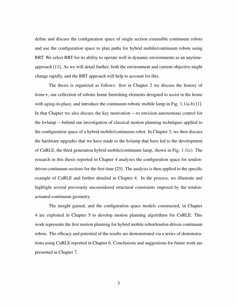
3.1 Third generation continuum robotic mobile lamp (CuRLE) with internalLED stip lit. . . . . . . . . . . . . . . . . . . . . . . . . . . . . . . . . . . 19

3.2 The full base of CuRLE. . . . . . . . . . . . . . . . . . . . . . . . . . . . 213.3 The central structure of CuRLE that houses all of the electronics is shown

with the motor plate removed. . . . . . . . . . . . . . . . . . . . . . . . . 23

vii

3.4 The assembled center structure with different electronic components vis-able. (a) The Raspberry Pi. (b) The Arduino Due (c) Voltage regulator(bottom) and motor drivers (top) . . . . . . . . . . . . . . . . . . . . . . . 24

3.5 The two main electronics plates removed from the central structure.(a) Topplate. (b) Left-half and (c) right-half of bottom plate. . . . . . . . . . . . . 24

3.6 (a) The turntable mechanism of CuRLE. (b) Zoomed in view of the con-nection between the worm drive and the turntable. . . . . . . . . . . . . . . 25

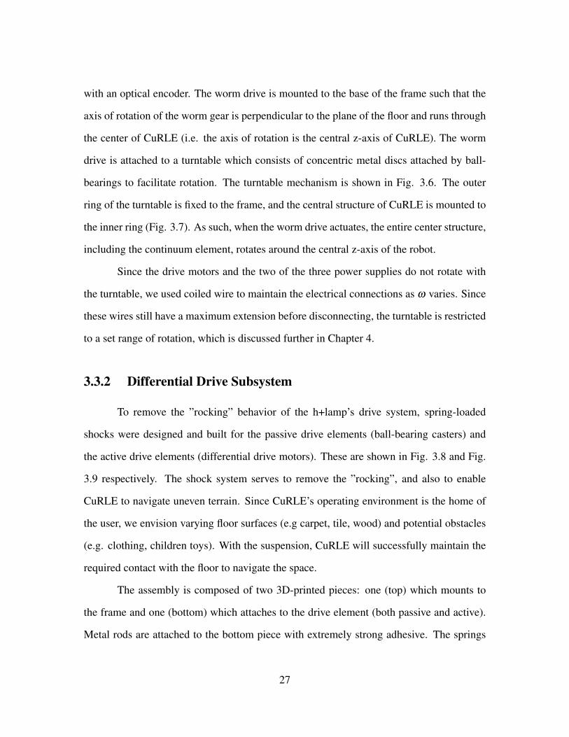
3.7 The central structure mounted on the turntable mechanism. . . . . . . . . . 263.8 (a) Top-side view of the passive drive element showing the through-holes

for the metal rods that provide stability and alignment in the shocks. (b)Side view of the shock assembly mounted to the ball-bearing casters (pas-sive drive element). . . . . . . . . . . . . . . . . . . . . . . . . . . . . . . 28

3.9 (a) Side view (under frame) of the shock assembly for one differential drivemotor. (b) In-line view of the drive motor shock assembly. (c) Side view(outside frame) of the shock assembly for the drive motor. . . . . . . . . . . 29

3.10 The motor plate which is mounted to the top of the central structure. Hereis where the tendon motors are mounted with the tension sensors and thespools to wind the tendons and measure length. . . . . . . . . . . . . . . . 31

3.11 (a) The 3D-printed assembly of a single tendon motor . . . . . . . . . . . . 323.12 (a) The gripper mounted as CuRLE’s end-effector with the LED lights lit

and the flexible grasping ”fingers” removed. (b) The gripper with the ”fin-gers” added. . . . . . . . . . . . . . . . . . . . . . . . . . . . . . . . . . . 34

3.13 The power system of CuRLE. (top) 4S LiPo battery to power the electron-ics. (middle) 4S LiPo battery to power the LEDs, LED strip, and servomotors in the gripper. (bot) 4S LiPo battery (later replaced with a 6S) topower all of the motors. . . . . . . . . . . . . . . . . . . . . . . . . . . . 36

4.1 An example of a single section extensible continuum robot [2]. . . . . . . . 394.2 A simple sketch demonstrating the kinematic variables of a single section

extensible continuum element. . . . . . . . . . . . . . . . . . . . . . . . . 404.3 Single section continuum robot bending (a) counter-clockwise and (b) clock-

wise in the yz-plane. . . . . . . . . . . . . . . . . . . . . . . . . . . . . . . 414.4 A visualization of C2

space. The blue plane extends to ±∞. The red circleindicates C2

space with the physical constraint of θ ≤ 2π . . . . . . . . . . . . 424.5 A visualization of C3

space. The dotted lines bordering the solid and the ar-rows indicate that u,v→ (±∞) and s→ (+∞). The prism is bounded bythe plane s = 0. . . . . . . . . . . . . . . . . . . . . . . . . . . . . . . . 42

4.6 An illustration of physical constraints of bending a continuum robot. In(a), L1 = L2 = s. In (b), the robot has bent counter-clockwise, causing L2to lengthen and L1 to shorten, while s remains constant. . . . . . . . . . . . 44

viii

4.7 A visualization of C3space. In (a) the physical constraints of the backbone

are illustrated. The maximum bend can be achieved when s = smax−smin2 ,

which is the widest plane in the center of the pyramid. In (b), the physicalconstraint of θ ≤ 2π is applied to (a), which forms the “rounded” pyramidshape. The largest “uv-plane” indicated circle in (b) is the same circleshown in Fig. 4.4. . . . . . . . . . . . . . . . . . . . . . . . . . . . . . . . 45

4.8 A sketch showing (a) the task-space-equivalent rigid-link RRPRR robot inthe same configuration(s) as (b) the continuum element. This is the resultof the kinematic mapping F . . . . . . . . . . . . . . . . . . . . . . . . . . 46

4.9 The task space of both the continuum section (black) and rigid link structure(green) for different values of u for the continuum section and [θ1, d] forthe rigid-link robot. . . . . . . . . . . . . . . . . . . . . . . . . . . . . . . 47

4.10 Q2space of the rigid-link robot.The arrows indicate the “wrapping” phenomenon

that occurs when θ1 and θ2 go beyond the bounds [0,2π). . . . . . . . . . . 474.11 A visualization of Q2

space of the rigid-link robot to show the “wrapping”phenomenom. A configuration q is any point on the surface. Changingθ1 “rotates” q around the axis, ac, running through the center of the torus.Changing θ2 “rotates” q around at which is the tangent to the path of rota-tion of θ1. . . . . . . . . . . . . . . . . . . . . . . . . . . . . . . . . . . . 48

4.12 Q3space of the rigid-link robot. The arrows indicate the “wrapping” phe-

nomenon that occurs when θ1 and θ2 go beyond the bounds [0,2π). . . . . 494.13 The configuration space (red) of the rigid-link structure, QC

space, once it hasbeen restricted by F to have the equivalent task space as the continuumsection. This is displayed within the full c-space (blue), Q3

space, from Fig.4.12 . . . . . . . . . . . . . . . . . . . . . . . . . . . . . . . . . . . . . . 52

4.14 Cspace of CuRLE. . . . . . . . . . . . . . . . . . . . . . . . . . . . . . . . 544.15 CuRLE’s base is a square frame with rounded corners. The radius of the

”disc” used to estimate the base of CuRLE is shown in green. . . . . . . . 56

5.1 Plots showing the different graphs through the simulated environment fordifferent types of RRTs. The path started at the green node and followed theyellow path to the magenta goal node, avoiding the configuration obstaclesdefined by the slashed lines surrounding the red obstacles in the task space. 62

5.2 Plot showing the RRT (type=VERTEX) expanding into an open environ-ment (no obstacles). The green node indicates the start. . . . . . . . . . . . 63

5.3 (a) RRT Experiment 1 Results. (b) RRT Experiment 2 Results. . . . . . . . 655.4 The configuration space of the mobile base in the scenario presented above . 675.5 The RRT growth over time. . . . . . . . . . . . . . . . . . . . . . . . . . . 715.6 A progression of images showing the simulated robot moving through the

scenario. . . . . . . . . . . . . . . . . . . . . . . . . . . . . . . . . . . . . 725.7 The task space showing the cup from the scenario. The middle cup is the

”goal” cup that CuRLE will pick up and deliver to the user. . . . . . . . . . 73

ix

5.8 The configuration space obstacles of the task space. The start configuration,is shown in (a), while (b) is the magnified obstacle from (a) where the goalconfiguration is located. (b) is the c-space obstacle of the shelf shown inFig. 5.7 . . . . . . . . . . . . . . . . . . . . . . . . . . . . . . . . . . . . 73

5.9 The interactive GUI that serves as the front end for simulation environment. 745.10 The simulated CuRLE in the start (vertical) and goal (bent) configuration.

The objective of the scenario was to pick up the cup, shown as a light greyprism, on the shelf. . . . . . . . . . . . . . . . . . . . . . . . . . . . . . . 75

6.1 (a) The state of CuRLE after ω has aligned with the goal ω . (b) CuRLEhas grasped the cup. (c) The results of a second path generated by the RRT(shown in Fig. 6.11) that guided CuRLE to pick the cup off the shelf. . . . . 80

6.2 The in-home scenario explored to demonstrate the full functionality ofCuRLE. The Locations discussed below are numbered in the image. Thefirst shelf is located at Location 2 and the second shelf is at Location 3. . . . 81

6.3 Output of the RRT showing the path required for the mobile base of CuRLEto navigate from the start location to the first shelf. . . . . . . . . . . . . . . 82

6.4 Output of the RRT showing the path required for CuRLE to grasp the cupon the first shelf. (b) is a magnified portion (a) to better show the start andgoal configurations. . . . . . . . . . . . . . . . . . . . . . . . . . . . . . . 82

6.5 Output of the RRT showing the path required for CuRLE to pick the cup upoff the first shelf. (b) is a magnified portion (a) to better show the start andgoal configurations. . . . . . . . . . . . . . . . . . . . . . . . . . . . . . . 83

6.6 (a-b) Results from Sub-Scenario 1 showing the execution of the RRT fromFig. 6.3 for the mobile base (i.e. CuRLE move from Location 1 to Location2). . . . . . . . . . . . . . . . . . . . . . . . . . . . . . . . . . . . . . . . 86

6.7 (a-b) Results from Sub-Scenario 1 showing the execution of the RRT fromFig. 6.4 (i.e. CuRLE grasp cup). . . . . . . . . . . . . . . . . . . . . . . . 87

6.8 (a) Results from Sub-Scenario 1 showing the execution of the RRT fromFig. 6.5 (i.e. CuRLE lift cup off shelf). (b) Results from Sub-Scenario 2showing the execution of the RRT from Fig. 6.9. . . . . . . . . . . . . . . . 88

6.9 Output of the RRT showing the path required for the mobile base of CuRLEto navigate from the first shelf to the second shelf. . . . . . . . . . . . . . . 89

6.10 Output of the RRT showing the path required for CuRLE to place the cupon the second shelf.(b) is a magnified portion (a) to better show the startand goal configurations. . . . . . . . . . . . . . . . . . . . . . . . . . . . . 89

6.11 Output of the RRT showing the path required for CuRLE to release the cupon the shelf and move away.(b) is a magnified portion (a) to better show thestart and goal configurations. . . . . . . . . . . . . . . . . . . . . . . . . . 90

6.12 (a-b) Continued results from Sub-Scenario 2 showing the execution of theRRT from Fig. 6.9 for the mobile base (i.e. CuRLE move from Location 2to Location 3). . . . . . . . . . . . . . . . . . . . . . . . . . . . . . . . . . 91

x

6.13 (a-b) Results from Sub-Scenario 2 showing the execution of the RRT fromFig. 6.10 (i.e. CuRLE release the cup). . . . . . . . . . . . . . . . . . . . . 92

6.14 Output of the RRT showing the path required for the mobile base of CuRLEto navigate from the second shelf to the ”docking station”. . . . . . . . . . 93

6.15 Output of the RRT showing the path required for CuRLE to return to its”home” state ([u = 0,v = 0,w = 0]) . . . . . . . . . . . . . . . . . . . . . . 94

6.16 (a-b) Results from Sub-Scenario 3 showing the execution of the RRT fromFig. 6.14 for the mobile base executing in parallel with the output of theRRT from Fig. 6.15 (i.e. CuRLE return to ”home” state while moving fromLocation 3 to Location 4). . . . . . . . . . . . . . . . . . . . . . . . . . . . 95

6.17 (a-b) Continued results from Sub-Scenario 3 demonstrating the parallel ex-ecution of the two RRTs. . . . . . . . . . . . . . . . . . . . . . . . . . . . 96

6.18 Final results of entire experimentation showing the small amount of errorin the final position of the mobile base. . . . . . . . . . . . . . . . . . . . . 97

xi

Chapter 1

Introduction

This thesis addresses the problem of motion planning for mobile robots featuring

novel continuum sections. We discuss the nature of the configuration space of, and its use

in motion planning for, continuum robots.

Continuum robots are composed of one or more continuum sections. A continuum

section is kinematically described by continuous and smooth curvature [3, 4]. Continuum

robots theoretically possess infinite degrees of freedom (DoF), unlike standard rigid-link

robots which have finite DoF. Continuum sections are most often tendon or pneumatically

driven, or composed of concentric tubes. These robots are often inspired by elements

in biology, such as plant tendrils, an elephant trunk, or octopus tentacles. Because of

their underlying curvature, continuum robots are often compliant in nature and are used to

explore hard-to-reach areas [5, 6].

Generating control algorithms for robots, including continuum robots, is a well-

studied problem, and multiple solutions are widely accepted and used [4, 7]. Often, these

robots are tele-operated and a lot of effort has been focused on intuitive control methods

for different robots [8, 9]. In contrast, autonomous motion requires motion planning.

Motion planning is the process of determining a path between two configurations

1

of the robot using its kinematics. A robot’s configuration can be described as vector of the

current value(s) of the independent kinematic variables of the robot. The set of all possible

configurations is the configuration space of the robot.

For conventional, non-continuum robots, classical motion planning techniques us-

ing configuration space have been well studied [10]. For example, rapidly exploring ran-

dom tree (RRT and RRT*) algorithms have been shown to successfully span the configu-

ration space for mobile robots and rigid-link robots [11, 12]. The A* algorithm, given a

graph and proper heuristic function, will guarantee the optimal path between any two nodes

if one exists [13].

In the past, a variety of motion planning techniques have been proposed for con-

tinuum robots. The motion planning problem for active cannulas (concentric tube robots

in medical applications) within tubular environments is formulated as an constrained opti-

mization problem in [14].

Constrained optimization is also used in [15] to formulate and solve the motion

planning problem for a soft planar continuum manipulator. Grasp planning for continuum

robots using a bounding circle technique was investigated in [16] and [17]. A follow the

leader approach for tendon-driven continuum robots is introduced in [18]. Researchers have

used sampling based approaches based on the techniques of Rapidly-Exploring Roadmaps

(RRM) [19], Rapidly-Exploring Random Graphs (RRG) [20, 21], and Rapidly-Exploring

Random Trees (RRT and RRT*) [22, 23] to plan motions for concentric tube continuum

robots in tubular environments for medical applications. RRTs are also used by [24] for

steering bevel-tip needles in 3D (medical) environments.

However, it appears that the principles of the classical motion planning techniques

such as RRT and A* have not yet been applied to tendon-actuated continuum robots in gen-

eral non-tubular environments. This is in part due to a lack of formal analysis of the nature

of the configuration space of tendon-actuated continuum robot elements. In this thesis, we

2

define and discuss the configuration space of single section extensible continuum robots

and use the configuration space to plan paths for hybrid mobile/continuum robots using

RRT. We select RRT for its ability to operate well in dynamic environments as an anytime-

approach [11]. As we will detail further, both the environment and current objective might

change rapidly, and the RRT approach will help to account for this.

The thesis is organized as follows: first in Chapter 2 we discuss the history of

home+, our collection of robotic home furnishing elements designed to assist in the home

with aging-in-place, and introduce the continuum robotic mobile lamp in Fig. 1.1(a-b) [1].

In that Chapter we also discuss the key motivation —to envision autonomous control for

the h+lamp —behind our investigation of classical motion planning techniques applied to

the configuration space of a hybrid mobile/continuum robot. In Chapter 3, we then discuss

the hardware upgrades that we have made to the h+lamp that have led to the development

of CuRLE, the third generation hybrid mobile/continuum lamp, shown in Fig. 1.1(c). The

research in this thesis reported in Chapter 4 analyzes the configuration space for tendon-

driven continuum sections for the first time [25]. The analysis is then applied to the specific

example of CuRLE and further detailed in Chapter 4. In the process, we illustrate and

highlight several previously unconsidered structural constraints imposed by the tendon-

actuated continuum geometry.

The insight gained, and the configuration space models constructed, in Chapter

4 are exploited in Chapter 5 to develop motion planning algorithms for CuRLE. This

work represents the first motion planning for hybrid mobile robot/tendon-driven continuum

robots. The efficacy and potential of the results are demonstrated via a series of demonstra-

tions using CuRLE reported in Chapter 6. Conclusions and suggestions for future work are

presented in Chapter 7.

3

Figure 1.1: The evolution of the continuum robotic mobile lamp element of the home+suite. (a) The original first generation lamp reported in [1]. (b) The second generation,called h+lamp, also described in [1]. (c) The third generation, called CuRLE (ContinuumRobotic Lamp Element) that forms the basis for this thesis.

4

Chapter 2

Home+ and the Second Generation

Continuum Robotic Mobile Lamp

This Chapter describes the first attempt at realizing the home+ continuum robotic

mobile lamp as an autonomous system. In doing so, we first discuss the key motivation

driving the home+ research project in more detail, and then describe how the work in this

thesis supports that effort.

2.1 In-Home Scenario

With the current societal move towards smart devices in every home, we envision a

collection of robotic furnishing elements that can provide at-home care and assistance. As

we age, we often lose the ability to perform simple day-to-day tasks and eventually reach a

point where we can no longer live without assistive care. Our suite of robots, collectively

called home+, are intended to collaborate with individuals over time in the home to help

with these day-to-day tasks and prolong the time that the individual can live independently

[1].

5

Figure 2.1: The home+ suite of robotic furnishing elements. (a) h+cube (b) h+lamp (c)h+armoire

We often envision at-home robotic care to be administered by fully functional,

android-esque robots such as those seen in cinema and dreamed of in science fiction. That

technology, however, has yet to be created, while many of the tasks that individuals need as-

sistance with can be accomplished by robotic technology that currently exists. For instance,

people need help retrieving objects from high shelves, so a continuum robotic mobile lamp

that includes the ability to do such tasks (in addition to functioning as a lamp) was devel-

oped prior to the work reported in this thesis. This first generation robot, shown in Fig. 2.2,

was added to the home+ suite. The other elements of home+ are a robotic end-table, or

”cube”, which is detailed in [1], and a robot ”armoire” (Fig. 2.1). These robots coordinate

together with the user to accomplish every-day tasks and assist the user with aging-in-place.

6

One of the key motivations driving the home+ effort has been to evaluate various

levels of user interaction with the suite of robots. For the work reported in this thesis, we

selected the continuum robotic mobile lamp experiment with the spectrum of user control.

To this end, we made extensive upgrades to allow for tele-operation and autonomous mo-

tion, as seen in Fig. 2.3 and 2.4. With this second generation robot, referred to as h+lamp

hereafter, we were able to conduct preliminary experiments to evaluate motion planning

for the mobile base.

2.1.1 Tele-Operation of h+lamp

On one end of the spectrum of control, the user is fully in command of the robot via

tele-operation, in which the user provides input to the robot via some form of user-interface.

The first generation lamp was controlled by a series of switches directly wired between the

power supply and the actuators [1]. Our initial upgrades moved this tethered, analog control

method to be wireless and digital. A hardware controller, shown in Fig. 2.5, received input

from the user and communicated the commands with wireless Bluetooth technology to the

robot. This was subsequently replaced with an Xbox360®controller communicating over

a wireless LAN connection by installing Wi-Fi enabling hardware into the h+lamp, shown

in Fig. 2.6. A central computer decoded input on the controller via C++ code which then

sent the commands to the robot over Wi-Fi.

2.1.2 Autonomous Motion of the h+lamp

The other end of the control spectrum is full autonomy of the robot. In this mode,

the user would give verbal, high-level commands, such as ”Bring me my cup.” and the

h+lamp would autonomously navigate (avoiding obstacles) to where the cup is stored, grab

the cup, and bring it back to the user. This is the mode the work in this thesis was intended to

7

Figure 2.2: First generation lamp hardware, as detailed in [1].

8

Figure 2.3: (a) The full replicated and upgraded hardware of the h+lamp. (b) A top-downview of the base of h+lamp showing the tendon motors and electronics. (c) A side-view ofthe of the base of h+lamp showing all of the electronics (i.e. Arduino Mega, motor drivers,voltage regulator, power supply, Wi-Fi shield)

9

Figure 2.4: A side-view of the h+lamp drive subsystem.

Figure 2.5: Tele-operation method of the h+lamp hardware using custom-built controllerand Bluetooth.

10

Figure 2.6: Tele-operation method of the h+lamp hardware using Xbox360®controller andwireless LAN.

enable. As a first attempt to do this, the passive mobile base (realized by steel ball-bearing

casters) was replaced with a differential drive system. This is detailed in section 2.2. To

implement full autonomy, sensing capabilities would have to be realized for the h+lamp to

recognize user input via voice command and detect the environment obstacles, in addition

to navigating the task space. The realization of this is beyond the scope of the project

reported in this thesis. As described later in Chapter 5, in this work the user’s commands

(i.e. the goal configurations) and the location of all obstacles are assumed known a priori

and we demonstrate progress towards autonomy with the novel motion planning algorithms

we developed.

2.2 Implementation of Path Planning for Mobile Base of

h+lamp

The differential drive system developed as part of this thesis work consisted of two

encoded DC gear-motors and a dual H-bridge motor driver controlled by PWM signals

from the Arduino Mega development board that functioned as the micro-controller for the

robot. The drive system, shown in Fig. 2.4, was powered by a 4S LiPo battery and step-

down voltage regulator, while the electronics were separately powered by 4 AA batteries.

11

Fig. 2.3 shows the h+lamp in this prototype version.

As mentioned earlier, the h+lamp connected to a central computer over Wi-Fi.

Rather than transmit user inputs from an Xbox360®controller, however, the central com-

puter ran the motion planning algorithms to autonomously move the robot from configura-

tion to configuration. These algorithms, RRT and A*, are detailed in Chapter 5.

The output of the RRT/A* algorithms was the path the robot must follow to reach

the goal. The path consisted of the set of actions U = {µ1,µ2, . . . µn}, which was wire-

lessly transmitted, one action at a time, to the robot via a TCP/IP socket connection. The

robot acknowledged the initial transmission (”init”) and began executing the actions as they

arrived. If a new action arrived before the robot finished its current action, the new action

was queued and executed next.

The motors were controlled by a PID controller implemented in the Arduino IDE.

As each action arrived, the robot calculated the new set-point of each wheel based on its

dynamics. A simple state-machine controled the flow of execution. The robot was idle

until it received the “init” command from the central computer. At this point, the robot

acknowledged the central computer and entered a waiting state until an action command

arrived. Once an action arrived, the robot moved through the action vector, first performing

a rotation, then translation, then the final rotation. Each individual movement was executed

by calculating the distance each wheel would travel. For a rotation, the distance σi traveled

by each wheel is given by Eqn. (2.1) where Lwheels is the distance between the wheels and

ϕi is the rotation of the current action.

σ1

σ2

=

ϕi ∗ Lwheels2

ϕi ∗ Lwheels2

(2.1)

12

For a translation, the distance δi traveled by each wheel is given by Eqn. (2.2) where

δ is the translation distance of the current action µ .

δ1

δ2

=

δ

δ

(2.2)

Either δi or σi was added to the current position of the wheel to give the desired

set-point for each wheel. The current position of each wheel p is given by Eqn. (2.3) where

Ecount is the current encoder count, Crev is the counts per revolution of the wheel, and rwheel

is the radius of the wheel.

p = Ecount ∗Crev ∗ rwheel ∗2π (2.3)

Once the desired set-point was calculated, the PID controller calculated the error

for each wheel and updated the velocity of the motors to move the error to zero. Once the

error was consistently below the minimum threshold value, the state-machine moved to the

next value of the action vector. If the action vector was complete and there were actions

waiting in the queue, the top value was popped out of the queue and execution began again;

otherwise the system moved back to the ready state awaiting the next action.

2.3 Results

After successfully running the RRT, watching the graph grow, and watching the

simulated robot successfully navigate the path (Chapter 5), we implemented the RRT on

the h+lamp. Before running the full path, the PID motor controller was thoroughly tested

13

Figure 2.7: The path for the h+lamp to follow through the in-home scenario experiment.

and tuned by serially sending the robot one action at a time. We also verified the state

machine logic and saw the robot successfully queue actions as it received them, executing

them in order one at a time. After placing the robot in the work space, which is shown in

Fig. 2.8, we executed the RRT and sent the path to the robot over Wi-Fi. The path for the

robot to follow is shown in Fig. 2.7. The best results of the robot executing this path are

shown in Fig. 2.9.

2.4 Analysis

The results revealed the need for improvements in the prototype hardware. The

robot began execution, but due to errors in the motor control, was not able to successfully

navigate to the goal. Errors in the motor control occured due to slight differences in the

velocities of the two different drive motors. For rotations, the velocities of the wheels were

not an issue and final position was reached. Since the PID control operated on errors in the

position, all rotations were successful. For translations, however, the unsensed velocities

14

Figure 2.8: A top-down view of the physical task space of the in-home scenario usedto validate the motion planning algorithms using the h+lamp robot hardware. The startlocation is shown in the top right in green with the goal location shown in the bottom leftin yellow. The configuration space obstacles are shown in blue.

15

Figure 2.9: A series of top-down views showing the h+lamp moving through the physicaltask space of the in-home scenario.

16

of the wheels matter significantly. If one wheel moves faster than the other, there will be

slight drift in the path towards the slower wheel. While the PID controller will force the

positional error to 0 for both wheels, this occurs at different times. The faster wheel stops

while other keeps moving. As a result, the robot ends up in the wrong position, and since

all the planning happens offline, the system is unable to sense and correct for the error and

does not update its trajectory as a result. As the errors accumulated, eventually the robot

collided with obstacles, (Fig. 2.9(c)) or left the work space (Fig. 2.9(b)).

Another significant cause of error occured due to the height mis-match between the

active drive elements (the wheels connected to the motors) and the passive drive elements

(the ball-bearing casters). In order to improve balance and stability, we added two passive

casters to the bottom of the h+lamp frame. We designed the casters to be the same height

as the wheel assembly, but due to the uneven surface of the task space floor, situations

arose where the passive elements maintained contact with the floor while the wheels were

”lifted” enough to cause slipping. To correct this, we significantly reduced the passive

element height, thereby sacrificing four points of contact with the floor for three, but guar-

anteeing that the wheels would always maintain contact with the floor. A by-product of

this modification was that robot would ”rock” back and forth around the wheel axis when

it accelerated. This caused further drift when executing the path from the RRT.

Our first attempt at validating the motion planning algorithms for the mobile base

was successful in the sense that robot received the commands and was able to serially

execute them. Due to hardware limitations and errors in the closed-loop control, the robot

did not accurately reach the goal. However, we showed that the motion planning algorithms

we developed allow the mobile base of the h+lamp to move through the task space. In the

next Chapter, we describe work done to fully upgrade the h+lamp to reduce the hardware

issues seen in this Chapter.

17

Chapter 3

Third Generation Continuum Robotic

Mobile Lamp: CuRLE

Given the problems observed during experimentation discussed in Chapter 2, we

constructed brand new robot hardware and installed upgraded features to solve the issues

we experienced, as well as to expand the capabilities of the robot. We named this third

generation robot CuRLE: Continuum Robotic Lamp Element, shown in Fig. 3.1. This

chapter describes our motivation for, and the details of, the extensive upgrades to produce

the new hardware.

3.1 Structural Overview

The structural hardware of CuRLE is comprised of three main components: the base

frame, the center structure, and the continuum backbone. The base frame, shown in Fig.

3.2 is built from aluminum beams and 3D-printed plastic corner pieces. The frame is square

with rounded corners. Mounted below the frame is a differential drive system, described

in section 3.3.2. Mounted inside to the bottom of the frame is a turntable mechanism,

18

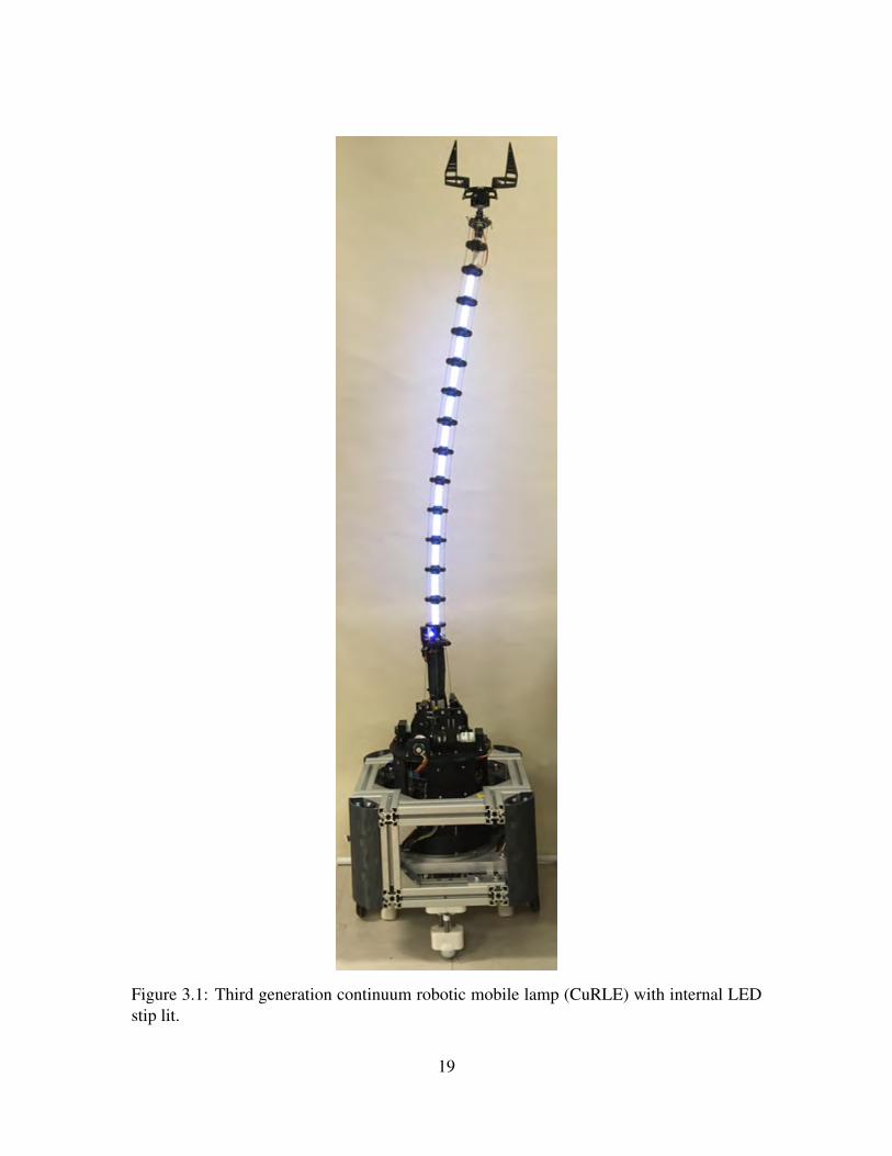
Figure 3.1: Third generation continuum robotic mobile lamp (CuRLE) with internal LEDstip lit.

19

described in section 3.3.1. Mounted on the turntable is the center structure.

The center structure is comprised of a 3D-printed plastic base plate, 3D-printed

walls, and a 3D-printed top plate. The linear actuator (the only vestigial hardware from the

h+lamp) is mounted to the base plate along with the bottom acrylic electronics plate (Fig.

3.5(b-c)). The walls attach to plastic struts that connect to the top and bottom plates. Small

protruding shelves can be attached to the inside of each wall, which support the top acrylic

electronics plate (Fig. 3.5(a)). All of the motor assemblies, described in section 3.3.3, are

mounted to the top plate of the center structure (i.e. the motor plate).

The continuum element is mounted at the end of the linear actuator and is comprised

of a PEX backbone (same material, but wider diameter than used for h+lamp’s backbone)

and new 3D-printed vertebrae. The actual ”lamp” features of CuRLE are comprised of

LED’s mounted to the final vertebra (i.e. the end-effector) and an LED strip that runs

through the backbone. These lighting features are described in section 3.3.5. Also mounted

to the end-effector is a gripper, detailed in section 3.3.4. The final subsystem is the power

system, described in section 3.3.6, which is mounted to the base of the frame.

3.2 Electronics Upgrades

To enable the hardware to execute as intended for the work in this thesis, the elec-

tronics of the h+lamp were necessarily upgraded. The Arduino Mega was replaced with the

Arduino Due, which has more computational power and higher clock speeds. The faster

clock is needed to enable the encoder counter chips, which replaced the old method of di-

rectly reading the encoders via interrupts on the Arduino. The new chips allow the Arduino

to focus its execution on other tasks (it no longer has to constantly handle interrupts from

the encoders) and reduce the number of digital pins required to interface with the motors.

To replace the Wi-Fi shield of the h+lamp, and eventually move CuRLE to a fully

20

Figure 3.2: The full base of CuRLE.

21

stand-alone unit, a Raspberry Pi was installed to serve as the ”central computer” for the

robot. Via remote wireless access, this computer serves as the connection point for the

robot and relays external commands to the Arduino via a hardware serial connection. The

Raspberry Pi can also relay traffic from the Arduino, enabling two-way communication

which was non-existent on the h+lamp. Figs. 3.3 and 3.4 show the electronics as they are

mounted within CuRLE.

All of the electronics, excluding those mounted to the continuum element and those

mounted beneath the center structure, are attached to the two acrylic plates shown in Fig.

3.5(a-c). The base plate holds the power electronics and the two computing devices (Rasp-

berry Pi computer and Arduino Due micro-controller). The top plate holds the encoder

counter chips, relay switches, and dual H-bridge motor drivers (same type as those in

h+lamp). The top plate also contains all the connection points for every motor (tendon,

turntable, and drive).

3.3 Details of the Hardware Upgrades

In the following sections, we describe the different hardware components of CuRLE.

3.3.1 Turntable

Since CuRLE needed to possess the capacity to autonomously execute the output

from motion planning algorithms developed for the continuum element (detailed later in

Chapter 4), we sought to fully separate the continuum c-space from the c-space of the mo-

bile base by adding a revolute joint at the base of the lamp. This joint allows the continuum

element to rotate independent of the movement of the mobile base. This added redundancy

creates new configuration opportunities for CuRLE.

The revolute joint, (variable ω), is realized by a worm drive run by DC gear-motor

22

Figure 3.3: The central structure of CuRLE that houses all of the electronics is shown withthe motor plate removed.

23

Figure 3.4: The assembled center structure with different electronic components visable.(a) The Raspberry Pi. (b) The Arduino Due (c) Voltage regulator (bottom) and motordrivers (top)

Figure 3.5: The two main electronics plates removed from the central structure.(a) Topplate. (b) Left-half and (c) right-half of bottom plate.

24

Figure 3.6: (a) The turntable mechanism of CuRLE. (b) Zoomed in view of the connectionbetween the worm drive and the turntable.

25

Figure 3.7: The central structure mounted on the turntable mechanism.

26

with an optical encoder. The worm drive is mounted to the base of the frame such that the

axis of rotation of the worm gear is perpendicular to the plane of the floor and runs through

the center of CuRLE (i.e. the axis of rotation is the central z-axis of CuRLE). The worm

drive is attached to a turntable which consists of concentric metal discs attached by ball-

bearings to facilitate rotation. The turntable mechanism is shown in Fig. 3.6. The outer

ring of the turntable is fixed to the frame, and the central structure of CuRLE is mounted to

the inner ring (Fig. 3.7). As such, when the worm drive actuates, the entire center structure,

including the continuum element, rotates around the central z-axis of the robot.

Since the drive motors and the two of the three power supplies do not rotate with

the turntable, we used coiled wire to maintain the electrical connections as ω varies. Since

these wires still have a maximum extension before disconnecting, the turntable is restricted

to a set range of rotation, which is discussed further in Chapter 4.

3.3.2 Differential Drive Subsystem

To remove the ”rocking” behavior of the h+lamp’s drive system, spring-loaded

shocks were designed and built for the passive drive elements (ball-bearing casters) and

the active drive elements (differential drive motors). These are shown in Fig. 3.8 and Fig.

3.9 respectively. The shock system serves to remove the ”rocking”, and also to enable

CuRLE to navigate uneven terrain. Since CuRLE’s operating environment is the home of

the user, we envision varying floor surfaces (e.g carpet, tile, wood) and potential obstacles

(e.g. clothing, children toys). With the suspension, CuRLE will successfully maintain the

required contact with the floor to navigate the space.

The assembly is composed of two 3D-printed pieces: one (top) which mounts to

the frame and one (bottom) which attaches to the drive element (both passive and active).

Metal rods are attached to the bottom piece with extremely strong adhesive. The springs

27

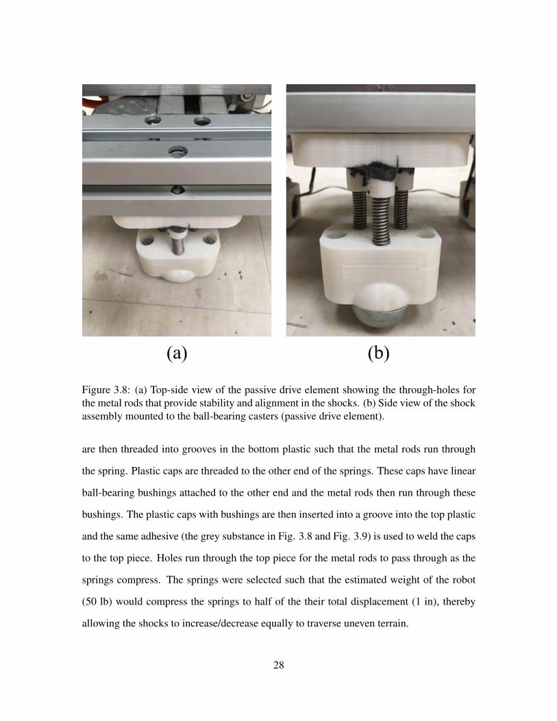
Figure 3.8: (a) Top-side view of the passive drive element showing the through-holes forthe metal rods that provide stability and alignment in the shocks. (b) Side view of the shockassembly mounted to the ball-bearing casters (passive drive element).

are then threaded into grooves in the bottom plastic such that the metal rods run through

the spring. Plastic caps are threaded to the other end of the springs. These caps have linear

ball-bearing bushings attached to the other end and the metal rods then run through these

bushings. The plastic caps with bushings are then inserted into a groove into the top plastic

and the same adhesive (the grey substance in Fig. 3.8 and Fig. 3.9) is used to weld the caps

to the top piece. Holes run through the top piece for the metal rods to pass through as the

springs compress. The springs were selected such that the estimated weight of the robot

(50 lb) would compress the springs to half of the their total displacement (1 in), thereby

allowing the shocks to increase/decrease equally to traverse uneven terrain.

28

Figure 3.9: (a) Side view (under frame) of the shock assembly for one differential drivemotor. (b) In-line view of the drive motor shock assembly. (c) Side view (outside frame)of the shock assembly for the drive motor.

3.3.3 Tendon Motors

To simplify the continuum kinematics, we modified CuRLE to a 4-tendon contin-

uum section compared to the 3-tendon design in h+lamp. The new kinematics are detailed

in section 3.4. With four tendons instead of three, control of only u and only v is possible by

actuating a single pair of tendons. This, in a addition to new revolute variable ω detailed

in section 3.3.1, allows us to easily restrict v to be constant (specifically v = 0) and still

achieve a desirable workspace. The use and advantage of this will be discussed in Chapter

4.

The hardware to attach the motors was upgraded from that in the h+lamp to account

for the increased motor count. In addition, we modified the spools the tendons wind around

to more accurately measure and track the length of the tendon. We also added a tension

sensing subsystem to prevent slack from developing in the tendons. Each motor assembly,

consisting of a DC gear-motor with optical encoder, 3D-printed mount, 3D-printed spool,

29

tension sensor, and 3D-printed tension sensor mount, is mounted at a 90o offset from its

neighbors and is shown in Fig. 3.11(a). All four motor assemblies are attached to the top

plate of the center structure, shown in Fig. 3.10.

3.3.3.1 Tension Sensors

Because the kinematics rely on accurately tracking the length of the tendons, it

is essential that the tendons do not develop slack. Change in tendon length is calculated

from the change in the motor encoder count based on the current circumference of the

tendon spool. Slack in the tendon causes the amount of tendon spooled to be less than

the amount reported by the motor encoder, thereby forcing the controller to evolve the

continuum element into a shape that is not accurately defined by its current configuration.

The tension sensor consists of a spring-loaded linear potentiometer mounted in-

line with the tendon. The tendon is threaded through an enclosed ”spool”, shown in Fig.

3.11(b), that is attached to the end of the tension sensor. Tension in the tendon compresses

the potentiometer, and slack allows the it to extend. By keeping the ”tension” reading

above a suitably selected threshold, a controller keeps slack out of the tendon and enables

accurate changes to CuRLE’s configuration.

3.3.3.2 Tendon Spools

To accurately a measure change in tendon length, we measure how much of the ten-

don has wound/unwound from the spool by calculating the change in the motor’s encoder

counts. Knowing the ratio of counts measured (∆Ecnt as determined by the encoder counter

chips mentioned in section 3.2) to counts per revolution (CPR) of the motor shaft and the

30

Figure 3.10: The motor plate which is mounted to the top of the central structure. Here iswhere the tendon motors are mounted with the tension sensors and the spools to wind thetendons and measure length.

31

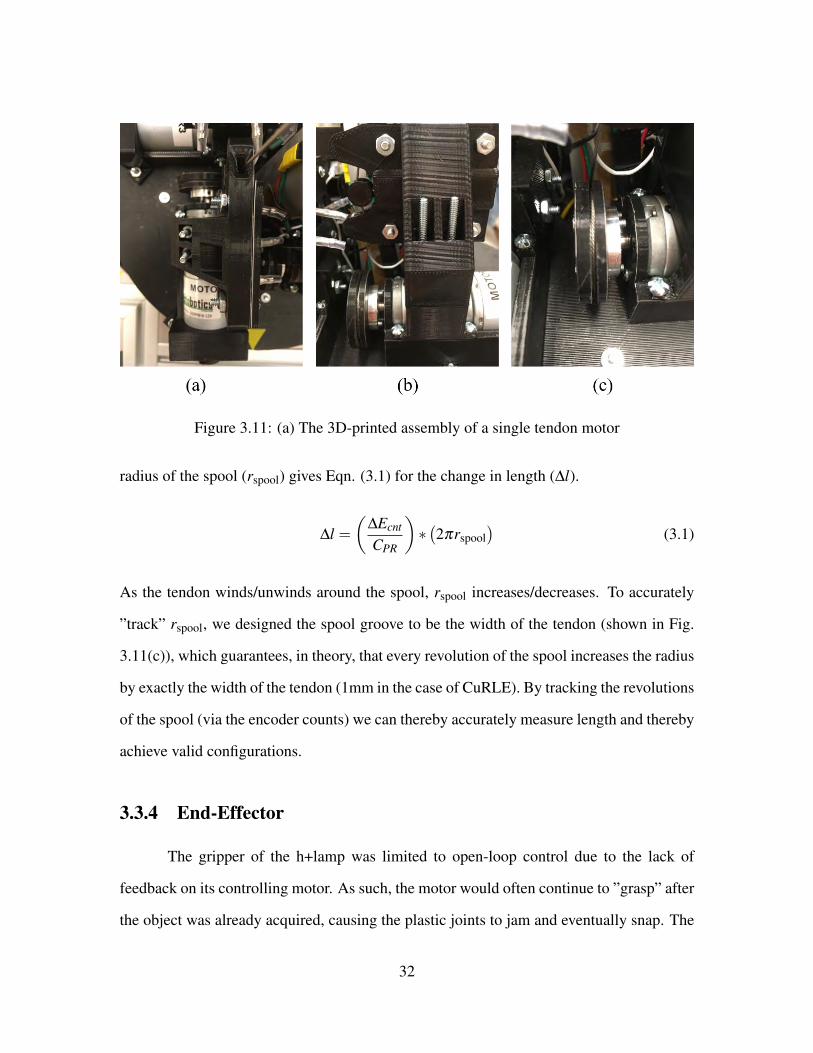
Figure 3.11: (a) The 3D-printed assembly of a single tendon motor

radius of the spool (rspool) gives Eqn. (3.1) for the change in length (∆l).

∆l =(

∆Ecnt

CPR

)∗(2πrspool

)(3.1)

As the tendon winds/unwinds around the spool, rspool increases/decreases. To accurately

”track” rspool, we designed the spool groove to be the width of the tendon (shown in Fig.

3.11(c)), which guarantees, in theory, that every revolution of the spool increases the radius

by exactly the width of the tendon (1mm in the case of CuRLE). By tracking the revolutions

of the spool (via the encoder counts) we can thereby accurately measure length and thereby

achieve valid configurations.

3.3.4 End-Effector

The gripper of the h+lamp was limited to open-loop control due to the lack of

feedback on its controlling motor. As such, the motor would often continue to ”grasp” after

the object was already acquired, causing the plastic joints to jam and eventually snap. The

32

new gripper’s ”grasping” mechanism is controlled by a servo motor with built-in position

control. By varying the duty cycle of the controlling PWM signal, this gripper will evolve

its configuration and hold a specified position.

The new gripper, seen in Fig. 3.12(a-b), also contains second servo motor (identical

to the first) that functions as a ”wrist” for the end-effector. The wrist (variable γ) enables

the gripper to grasp items in configurations that its predecessor could not. The nature of

continuum element kinematics allows for a wide set of end-effector Cartesian locations,

but few in this set orient the end-effector in a convenient way to grasp objects. The ability

to rotate the end-effector via the wrist increases the set.

The final upgrades to the gripper are flexible ”finger” attachments that enhance

grasping. The ”fingers” are 3D printed using a flexible thermoplastic polyurethane material

that wraps around an object when the claw grasps it. These ”fingers” are shown in Fig.

3.12(b).

3.3.5 Lighting Elements

Fig. 3.12(b) shows the LED’s mounted on the end-effector to realize CuRLE’s

function as a lamp. There are eight 9mm white LEDs connected in parallel with a 5V

source. A digital switch controlled by the Arduino Due toggles the LED’s. In addition, an

LED strip was run down the center of the PEX backbone to provide more lighting to the

user. The lit LED strip is shown in Fig. 3.1.

3.3.6 Power Subsystem

Since CuRLE now possess more actuators and electronics than its predecessor, we

installed additional power supplies to robot. The 4S LiPo battery used to power the motors

in h+lamp (see Chapter 2) was replaced with a 6S LiPo with a greater capacity. The same

33

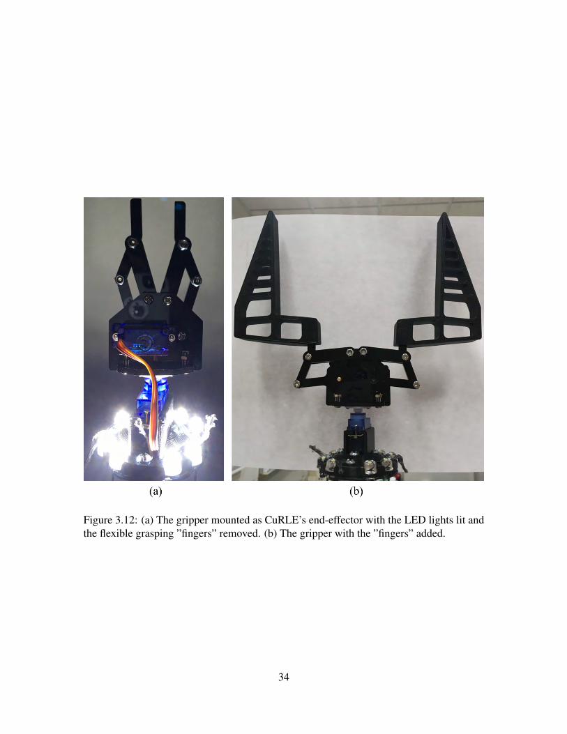
Figure 3.12: (a) The gripper mounted as CuRLE’s end-effector with the LED lights lit andthe flexible grasping ”fingers” removed. (b) The gripper with the ”fingers” added.

34

12V switching voltage regulator provides a constant DC supply to the drive motors, linear

actuator, tendon motors, and worm drive motor. The 4 AA batteries used to power the

electronics in h+lamp were replaced with a 4S LiPo battery to power the new electronics in

CuRLE. This supply is passed to two separate voltage regulators, one that provides 12V and

one that provides 5V, to power the Arduino Due and Raspberry Pi, respectively. Finally,

we installed a third 4S LiPo battery to power the new LED strips and the servo motors of

the gripper. This battery is also connected to a 12V (LED strip) and a 5V (LED’s and servo

motors) voltage regulators. Fig. 3.13 shows the power supplies of CuRLE.

3.4 Kinematics

We next present the kinematics for a single section 4-tendon continuum section.

While these equations hold for the more general case of an extensible section, the arc

length s of the continuum element remains fixed in CuRLE. The tendons are arranged such

that tendons 1 and 3 (variables l1 and l3) are an opposing pair in the v-plane (u = 0) and

tendons 2 and 4 (variables l2 and l4) are an opposing pair in the u-plane (v = 0).

l1 = s+(−d) · v (3.2)

l2 = s+(d) ·u (3.3)

l3 = s+(d) · v (3.4)

l4 = s+(−d) ·u (3.5)

35

Figure 3.13: The power system of CuRLE. (top) 4S LiPo battery to power the electronics.(middle) 4S LiPo battery to power the LEDs, LED strip, and servo motors in the gripper.(bot) 4S LiPo battery (later replaced with a 6S) to power all of the motors.

36

l1

l2

l3

l4

=

0 −d 1

d 0 1

0 d 1

−d 0 1

·

u

v

s

(3.6)

u =l2− l4

2d(3.7)

v =l3− l1

2d(3.8)

s =l1 + l3

2=

l2 + l42

=l1 + l2 + l3 + l4

4(3.9)

u

v

s

=( 1

4d

)−2 0 2 0

0 2 0 −2

d d d d

·

l1

l2

l3

l4

(3.10)

37

Chapter 4

Configuration Space of CuRLE

This chapter starts by defining for the first time the general configuration space for

a single section extensible continuum element [25]. We identify several interesting and

unique practical aspects of continuum section C-space, particularly in the case of tendon-

actuated sections. To highlight these unique aspects of continuum robots, we compare to

this configuration space with that of a rigid-link robot that is selected to have a similar task

space. We then discuss the constraints to the continuum configuration space that are im-

posed by the physical construction of CuRLE. Finally, we discuss the configuration space

of CuRLE’s mobile base, and how we can isolate it from the configuration space of the

continuum section by making suitable assumptions about the task space.

4.1 Continuum Configuration Space

We begin by considering the underlying structure of continuum robot configuration

space in the presence of physical and actuation constraints. Specifically, we consider the

c-space of the basic element of continuum robots: a single extensible section. We assume

the section to be of constant curvature, a common assumption in the literature [4].

38

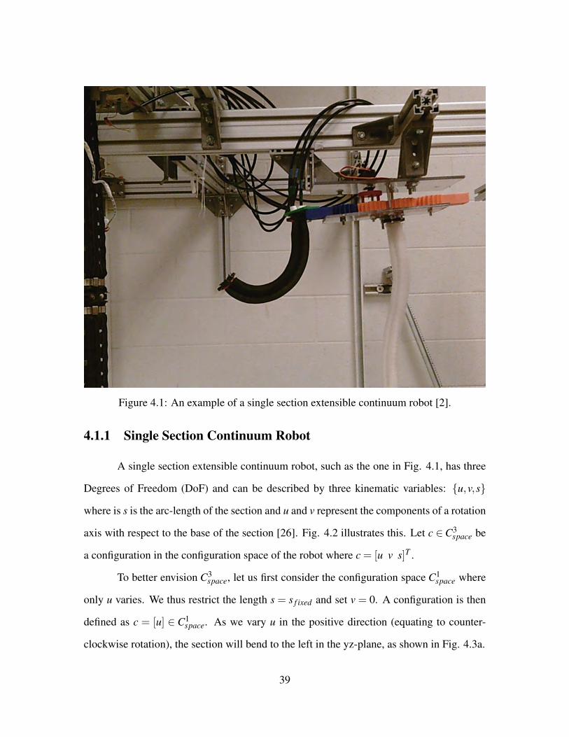
Figure 4.1: An example of a single section extensible continuum robot [2].

4.1.1 Single Section Continuum Robot

A single section extensible continuum robot, such as the one in Fig. 4.1, has three

Degrees of Freedom (DoF) and can be described by three kinematic variables: {u,v,s}

where is s is the arc-length of the section and u and v represent the components of a rotation

axis with respect to the base of the section [26]. Fig. 4.2 illustrates this. Let c ∈C3space be

a configuration in the configuration space of the robot where c = [u v s]T .

To better envision C3space, let us first consider the configuration space C1

space where

only u varies. We thus restrict the length s = s f ixed and set v = 0. A configuration is then

defined as c = [u] ∈ C1space. As we vary u in the positive direction (equating to counter-

clockwise rotation), the section will bend to the left in the yz-plane, as shown in Fig. 4.3a.

39

y

v

u

s

z

x

Figure 4.2: A simple sketch demonstrating the kinematic variables of a single section ex-tensible continuum element.

Once u = 2π , the section’s tip will meet the base and form a perfect circle. Contin-

uing to increase u will cause the robot to “bend within itself”’ and theoretically it would

continue to “encircle” itself as u→ ∞. Increasing u in the negative direction (clockwise)

will cause the same planar motion mirrored across the z-axis (Fig 4.3b). As u→ (−∞),

the robot will continue to encircle itself to generate the remaining set of possible planar

configurations of the section. Therefore, the configuration space of the robot where only u

varies is C1space ≡ R.

If we remove the restriction on v and allow it to also vary, then the configuration

space changes to a 2D space where any configuration is defined as c = [u v]T ∈C2space. The

40

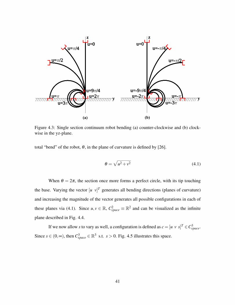
u=0 u= /4

u= /2

u= u=2u=9 /4

u=3

z

y

u=0 u=- /4

u=- /2

u=-u=-2u=-9 /4

u=-3

z

y

(a) (b)

Figure 4.3: Single section continuum robot bending (a) counter-clockwise and (b) clock-wise in the yz-plane.

total “bend” of the robot, θ , in the plane of curvature is defined by [26].

θ =√

u2 + v2 (4.1)

When θ = 2π , the section once more forms a perfect circle, with its tip touching

the base. Varying the vector [u v]T generates all bending directions (planes of curvature)

and increasing the magnitude of the vector generates all possible configurations in each of

these planes via (4.1). Since u,v ∈ R, C2space ≡ R2 and can be visualized as the infinite

plane described in Fig. 4.4.

If we now allow s to vary as well, a configuration is defined as c= [u v s]T ∈C3space.

Since s ∈ (0,∞), then C3space ∈ R3 s.t. s > 0. Fig. 4.5 illustrates this space.

41

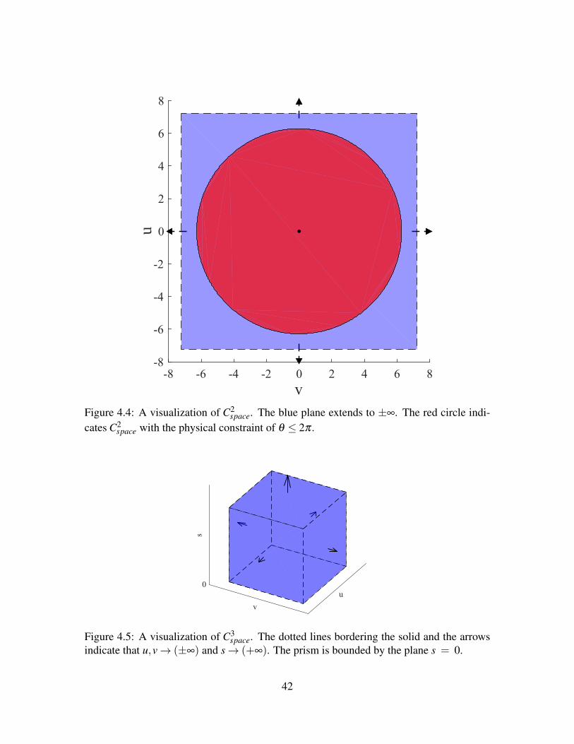
-8 -6 -4 -2 0 2 4 6 8v

-8

-6

-4

-2

0

2

4

6

8

u

Figure 4.4: A visualization of C2space. The blue plane extends to ±∞. The red circle indi-

cates C2space with the physical constraint of θ ≤ 2π .

uv

s

0

Figure 4.5: A visualization of C3space. The dotted lines bordering the solid and the arrows

indicate that u,v→ (±∞) and s→ (+∞). The prism is bounded by the plane s = 0.

42

4.1.2 Physical Constraints in a Single Section Continuum Robot

At this point, however, we introduce constraints in the configuration space imposed

by physical limitations of the robot. The first constraint to consider is on length. Any

physical robot will have a maximum and minimum length, imposing an upper and lower

bound on arc-length: smin ≤ s≤ smax.

Another constraint is imposed by the physical width of the backbone of tendon

actuated continuum robots. This physical distance, dr > 0, is the distance from the center

of the backbone to its outer edge. With s the length down the exact center of the backbone,

and L1 and L2 the tendon lengths along its outside in the plane of bending (Fig. 4.6), when

the robot is perfectly straight (i.e. u = v = 0), then L1 = L2 = s (Fig. 4.6a). For the robot

to bend counter-clockwise in the plane, the length of the left side of the robot, L2, must

shorten at the same rate that the length of the opposite side of the robot, L1, lengthens. This

is illustrated in Fig. 4.6b.

Because of this, the section cannot bend at all when it is at maximum or minimum

length. When s = smax and u = v = 0, then L1 = L2 = smax. To bend, L1 or L2 must

lengthen, but each is already at the maximum length. The same reasoning is applied when

s = smin. At maximum/minimum length, C3space = {

[0 0 smax/min

]T }. For intermediate

values of s, a similar situation holds —bending can occur up to one tendon achieving max

length. The practical configuration space can now be visualized in Fig. 4.7(a). When

s = smax−smin2 the robot will be able to achieve the greatest amount of bending and will have

the largest “uv-plane”.

This pyramid shape assumes there are a pair of opposing tendons in the u-plane

and another pair of opposing tendons in the v plane, which is consistent with the CuRLE

hardware. The flat surfaces of the pyramid reflect this alignment, meaning that if the pairs

tendons were rotated to align in other planes, the pyramid would rotate such that the flat

43

u = 0

dr

s L2

L1

z

y

u = /4

dr

s L2L

1

z

y

(b)(a)

Figure 4.6: An illustration of physical constraints of bending a continuum robot. In (a),L1 = L2 = s. In (b), the robot has bent counter-clockwise, causing L2 to lengthen and L1 toshorten, while s remains constant.

surfaces would face the tendon directions.

A further practical constraint arises due to “encircling” imposed when θ > 2π .

Given a specific physical construction of a practical continuum section, it is likely that

it will not be able to “encircle” itself. Even if it could, it cannot continue doing so as

u, v→ (±)∞. Therefore, there will exist some boundary for u and v imposed by physical

constraints. In this thesis, and consistent with our hardware, we set this boundary to be at

θ = 2π , which bounds C2space as shown in Fig. 4.4. Expanding the θ ≤ 2π constraint to

C3space gives the space seen in Fig. 4.7(b), which is the practical configuration space for a

single section extensible continuum robot with physical constraints exploited herein.

44

uv

sssmax

smin smin

smax

vu

(b)(a)

Figure 4.7: A visualization of C3space. In (a) the physical constraints of the backbone are

illustrated. The maximum bend can be achieved when s = smax−smin2 , which is the widest

plane in the center of the pyramid. In (b), the physical constraint of θ ≤ 2π is applied to(a), which forms the “rounded” pyramid shape. The largest “uv-plane” indicated circle in(b) is the same circle shown in Fig. 4.4.

4.2 A Comparison: Equivalent Rigid-Link Robot Config-

uration Space

To highlight the unique issues presented by continuum section structures, we com-

pare with the case of a kinematically similar rigid link robot.

4.2.1 Equivalent Rigid Link Robot

To analyze a rigid link robot structure with the same DoF as the continuum robot

section, we use for comparison a 3 DoF robot (Fig. 4.8) with a constrained RRPRR joint

configuration similar to the planar RPR robot described in [27].

In this, we constrain the third and fourth revolute joint angles to exactly match

the first and second revolute joint angles, respectively, which gives the configuration vector

q= [θ1 θ2 d θ1 θ2]T . The prismatic joint can extend/retract between known maximum and

45

y

x

z

y

x

z

(a) (b)

Figure 4.8: A sketch showing (a) the task-space-equivalent rigid-link RRPRR robot in thesame configuration(s) as (b) the continuum element. This is the result of the kinematicmapping F .

minimum lengths. We select this rigid link configuration since we can construct a kinematic

mapping between its configuration space and the configuration space of the continuum

robot section that restricts the rigid-link robot task space to the equivalent task space of the

continuum section. This mapping, F , is described in section 4.2.4. Fig. 4.9 shows the two

robots sharing the same task space.

46

z

y

Figure 4.9: The task space of both the continuum section (black) and rigid link structure(green) for different values of u for the continuum section and [θ1, d] for the rigid-linkrobot.

4.2.2 Rigid-Link Robot Configuration Space

-2 0 2 4 6 8

2 [rad]

-2

0

2

4

6

8

1 [ra

d]

Figure 4.10: Q2space of the rigid-link robot.The arrows indicate the “wrapping” phenomenon

that occurs when θ1 and θ2 go beyond the bounds [0,2π).

47

,Ii\, I •

'

I '

---�

2

1

ac

at

Figure 4.11: A visualization of Q2space of the rigid-link robot to show the “wrapping” phe-

nomenom. A configuration q is any point on the surface. Changing θ1 “rotates” q aroundthe axis, ac, running through the center of the torus. Changing θ2 “rotates” q around atwhich is the tangent to the path of rotation of θ1.

For the two independent revolute DoF: θ1,θ2 ∈ [0,2π) we define q = [θ1 θ2]T ∈

Q2space. Rather than the infinite plane in Fig. 4.4, the space manifests as a square with

a “wrapping” phenomenon that causes θ1,θ2 ≥ 2π,∨ θ1,θ2 < 0 to “wrap” back to 0 ≤

θ1,θ2 < 2π , as seen in Fig. 4.10. This space, while locally 2D, is globally best visualized

as the surface of a torus, like that in Fig. 4.11.

Adding the prismatic joint modifies the ”square” in Fig. 4.10 into the ”rectangular

prism” shown in Fig. 4.12. As with the Q2space, the same “wrapping” phenomenon occurs

whenever one of the joints goes beyond 0 or 2π . The configuration space can be defined as

∀q = [θ1 θ2 d]T ∈ Q3space s.t. 0≤ θ1 < 2π, 0≤ θ2 < 2π, dmin ≤ d ≤ dmax.

48

8

d

8664

1 [rad]

2 [rad]

42 20 0-2 -2

dmin

dmax

Figure 4.12: Q3space of the rigid-link robot. The arrows indicate the “wrapping” phe-

nomenon that occurs when θ1 and θ2 go beyond the bounds [0,2π).

4.2.3 C-Space of Continuum Section vs Rigid-Link Structure

The key difference between the continuum and rigid-link configuration spaces (c-

space) is the “wrapping” phenomenon that occurs in Q3space. In the ideal continuum c-space,

there exists exactly 1 straight path connecting any two configurations c1, c2 ∈C3space. For

the rigid-link robot, there are always 2 straight paths between any configurations that in-

volve a change in θ1 or θ2. For configuration changes that exclusively involve the prismatic

joint, there is exactly 1 path.

An interesting difference between the c-spaces is their sizes. Since both C3space and

Q3space are finite their sizes can be compared by calculating the volume of each space. This

can be done by calculating the volume of the 3D shapes shown in Fig. 4.7(b) and Fig. 4.12.

49

The size of Q3space is the volume of the rectangular prism. The size of C3

space is the volume

of the “rounded” pyramid, which is slightly less than the full 2- sided square pyramid but

greater than a 2-sided cone where the base has radius = 2π .

(4π2)(smax− smin)

(π

3

)<Vcont < (4π

2)(smax− smin)

(83

)Vrigid = (4π

2)(dmax−dmin) (4.2)

Since the rigid-link robot was chosen to be kinematically similar to the continuum

robot, we can conclude that the configuration space for a kinematically equivalent contin-

uum section is larger than the rigid-link robot’s configuration space (Eqn. 4.3).

smax = dmax , smin = dmin

⇒Vrigid <Vcont (4.3)

4.2.4 Ensuring Equivalent Task Spaces

The only difference between the two task spaces is the physical shape of the arm

of the robot that creates them. This is either a constant curvature curve between the base

and the end-effector (continuum) or a straight line (rigid-link), as shown in Fig. 4.9. This

shape, however, is important in the context of motion planning, as it has to be accounted

for when checking for collision-free paths through the space.

For the rigid-link robot to have the same task-space as the continuum robot, we

construct a function F that maps every configuration c ∈ C3space to a configuration q ∈

Q3space. This function, F , is neither one-to-one nor onto, and is shown in Eqn. (4.4).

50

F : C3space→ Q3

space s.t. F(c) = q where

c =

u

v

s

∈C3space and q =

θ1

θ2

d

∈ Q3space

⇒ F(c) =

u2

v2(

2s√u2+v2

)sin(√

u2+v2

2

) (4.4)

Let QCspace , R{F} where R{F} is the range of the function F . Then QC

space ∈

Q3space is a subspace of Q3

space. Since C3space is centered at u = v = 0, and has a radius of 2π ,

QCspace will be centered at θ1 = θ2 = 0. Now, we restrict θ1,θ2 such that

√θ 2

1 +θ 22 ≤ π .

This is the effect of applying F to Eqn. (4.1). If this is not done, then the value of d, as

described be Eqn. (4.4), would take on negative values, because of the sin(√

u2+v2

2

)term.

This restriction of θ1,θ2 also removes the “wrapping” phenomenon and causes QCspace to

have the same “rounded” pyramid shape as C3space, as shown in Fig. 4.13.

Finally, by comparing (4.2) and (4.4), the volume of QCspace is significantly smaller

than the volume of the C3space, but the task space is equivalent.

(π2)(smax− smin)(

π

3

)<Vequiv < (4π

2)(smax− smin)

(23

)(4.5)

51

12

dmax

dmin

d

Figure 4.13: The configuration space (red) of the rigid-link structure, QCspace, once it has

been restricted by F to have the equivalent task space as the continuum section. This isdisplayed within the full c-space (blue), Q3

space, from Fig. 4.12

4.3 Continuum Robotic Lamp Element: CuRLE

Recall from Chapter 3, CuRLE is a tendon-driven, non-extensible, single-section

continuum arm mounted onto a mobile base which is controlled by a differential drive.

CuRLE ’s end-effector is a 2-fingered gripper featuring a series of LEDs to give the lamp

light. Additional lighting is provided by LED strips inside the continuum body of the lamp.

The continuum arm is mounted on a prismatic joint (variable length L) which serves

to raise/lower the base of the continuum arm but does not change the continuum arc length

s. The prismatic joint is further mounted on a revolute joint (variable ω) which allows

the entire arm to be rotated about the z-axis (yaw). Another revolute joint (variable γ) is

mounted at the end of the continuum arm to serve as a “wrist” for the gripper.

4.3.1 Adding Constraints

In order to visualize the configuration space of CuRLE and conduct practical mo-

tion planning through the home environment space, we constrain several DoF. For the re-

52

mainder of this work, we fix L to its minimum length. Since the continuum arm is non-

extensible, the arc-length s is necessarily constrained to be constant. The revolute joint γ

serving as the wrist for the gripper adds redundancy, but remains fixed in the experimenta-

tion described here.

With these restrictions, we discuss the mobile base and the kinematic variables

[ω u v] for the continuum arm. Since the base serves to move the continuum lamp ele-

ment through the home space and the continuum element performs manipulation, we di-

vide the configuration space into two parts. We assume that there will not be obstacles

that CuRLE has to “pass under” meaning that nothing in the task space would collide with

the continuum arm but not the mobile base. As such, we form the configuration space of

the continuum arm c = [ω u v] ∈ Cspace and the configuration space of the mobile base

q = [x y θb]T ∈C base

space.

4.3.2 Configuration Space of CuRLE

Recall that for a fixed arc-length s, a single section continuum robot has a practical

configuration space of a circle bounded by θ = 2π , shown in Fig. 4.4. Since the continuum

arm of CuRLE can physically collide with the mobile base, we further modify the boundary

to θ ≤ π√

2 (the value of the θ when u = v = π).

The revolute joint at the base of the continuum arm is described by ω ∈ [0,2π).

In the ideal case, ω displays the same “wrapping” behavior that the revolute joints in the

rigid-link configuration space. As such, adding ω changes the configuration space to 3

dimensions by revolving the “uv-circle” around a central axis. The shape, depicted in Fig.

4.14, echoes the torus described by Q2space, the c-space of 2 revolute DoF. Unlike Q2

space,

however, CuRLE ’s is “solid”, i.e. true 3D, meaning that configurations c are not limited to

the surface of the torus only. ω selects the “slice” (a circle) of the torus and u and v select

53

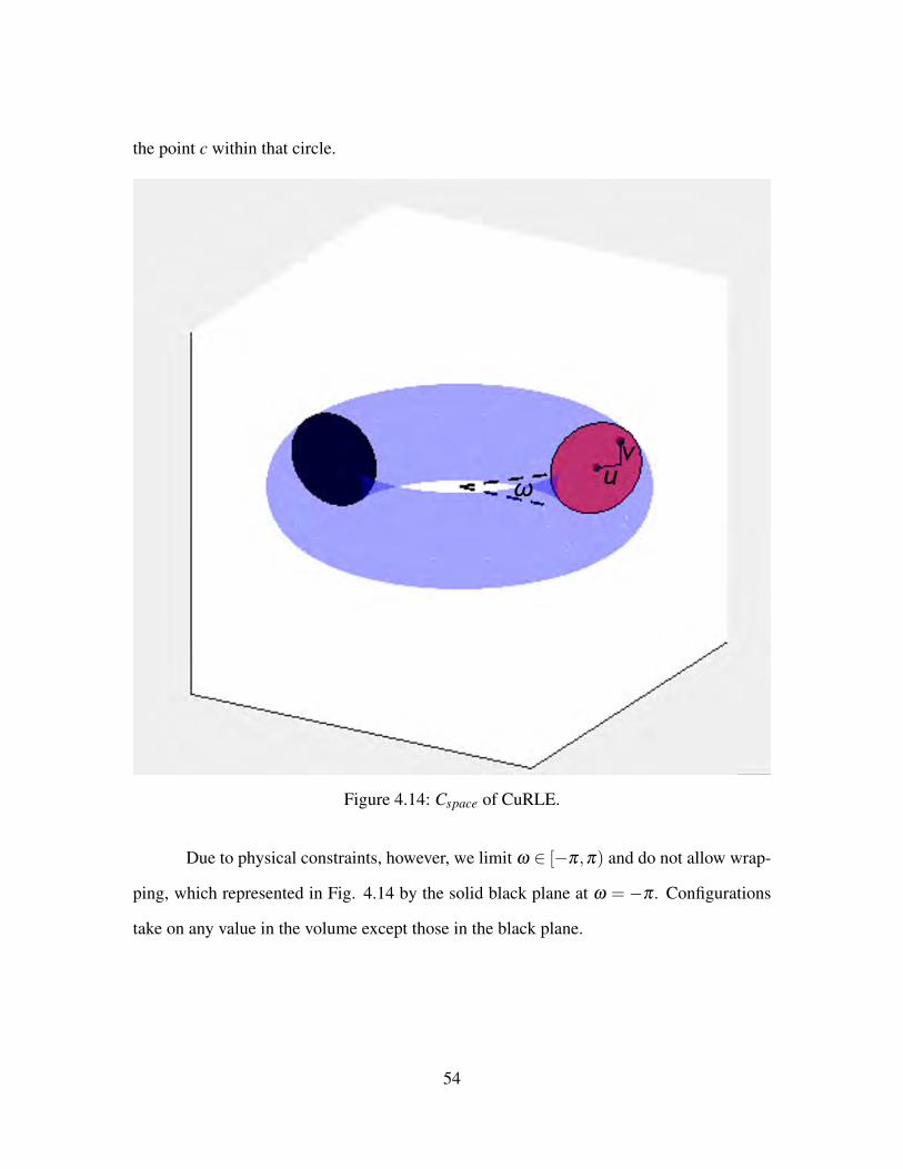
the point c within that circle.

Figure 4.14: Cspace of CuRLE.

Due to physical constraints, however, we limit ω ∈ [−π,π) and do not allow wrap-

ping, which represented in Fig. 4.14 by the solid black plane at ω = −π . Configurations

take on any value in the volume except those in the black plane.

54

4.4 Configuration Space of Mobile Base

Since we separate the configuration space of the continuum element from the C-

space of the mobile base by making the assumptions described above, we can formally

define the configuration space of the mobile base C basespace in (4.6) where q is a configuration

of the robot in the configuration space C basespace, x and y are the positions of the robot along the

x-axis and y-axis respectively, and θb ∈ [0,2π) is the orientation of the robot with respect

to the positive x-axis.

∀q ∈C basespace : q = [x y θb]

T (4.6)

The ideal configuration space (i.e. no physical constraints) has the shape of a rect-

angular prism with an infinite base (i.e. the x,y-plane) and a height, θb ∈ [0,2π), of 2π . In

any practical application, however, the parameters x and y will always be bounded by the

walls of the room.

Obstacles in this configuration space are described as the Minkowski difference of

the robot and the obstacle in the task space [11]. All the obstacles to the mobile base used in

our experiments were designed to be convex polygonal in shape, since collision-avoidance

can often be simplified by drawing a “bounding-box” around the obstacle. The base of

CuRLE is a rectangular box with rounded corners (Fig. 4.15) meaning that the obstacles

would resembled “twisted pillars” in the configuration space [13]. To again simplify the

design, the robot is treated as a disc with a diameter equal to the diagonal of the frame. With

the robot as a disc, collision detection can disregard θb and simply check for collisions in

the x,y-plane [10].

For the robot to move between two configurations, q0 and q1, an action vector µ is

55

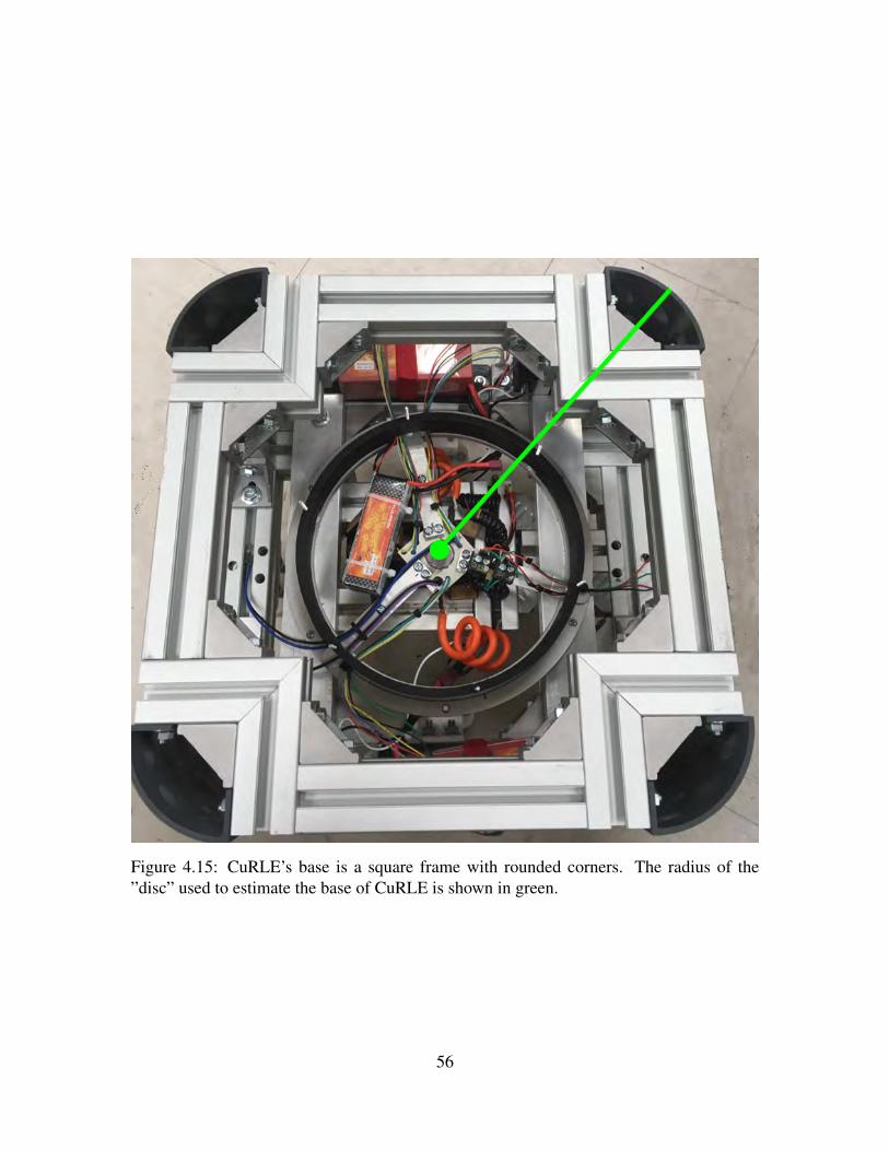
Figure 4.15: CuRLE’s base is a square frame with rounded corners. The radius of the”disc” used to estimate the base of CuRLE is shown in green.

56

defined in (4.7) based on the robot kinematics.

µ : q0→ q1,where q0 = [x0 y0 θ0]T and q1 = [x1 y1 θ1]

T

then µ = [ϕ1 δ ϕ2]T where

ϕ1 = min rot(

arctan(

y1− y0

x1− x0

)−θ0

)δ =

√(x1− x0)

2 +(y1− y0)2

ϕ2 = min rot(θ1−ϕ1) (4.7)

The min rot(ϕ) function in (4.7) returns the minimum rotation needed to move

between two angles. If the calculated rotation is greater in magnitude than π radians, then

a rotation in the opposite direction provides an overall shorter rotation. (i.e. a counter-

clockwise rotation might be shorter than rotating in a clockwise direction and vice versa).

The final aspect of defining the configuration space is a metric d(q0,q1) that defines

the “distance” between the two configurations q0 and q1 [13]. For CuRLE , the simplifi-

cations made to the configuration space allow the metric d(q0,q1) to be defined as the

Euclidean distance (L2-norm) between the x and y coordinates of the q0 and q1.

With the configuration spaces of the continuum element and the mobile base de-

fined, we now have the foundation to discuss the motion planning algorithms we developed

to navigate these spaces.

57

Chapter 5

Motion Planning

In this chapter, we introduce new motion planning algorithms specifically created

for CuRLE and simulations used to test and verify them. First, we discuss the RRT used

for the mobile base of the robot (Chapter 2), using the configuration space discussed in

Chapter 4. Next, we detail the simulation environment for the mobile base used to test the

algorithms’ output. This is the simulation from the discussion in Chapter 2 which was used

to verify the RRT before implementing on the h+lamp hardware.

We then discuss the necessary modifications made to the RRT to path plan for the

continuum arm element of the robot. The new simulated environment developed to test

this second algorithm is also described. Finally, we will show how the two RRTs can

be combined to run in parallel and provide the results for those (simulated) experiments.

The physical implementations corresponding to these simulated tests will be discussed in

Chapter 6.

58

5.1 Path Planning for the Mobile Base

5.1.1 Rapidly-Exploring Random Tree (RRT) Algorithm

An RRT is a probabilistic approach to motion planning [11]. The objective is to

connect a pre-defined start configuration with a desired goal location by constructing a tree

of randomly selected nodes from the configuration space. The RRT is an iterative process

that rapidly expands to cover the free-space of an environment. At each iteration, a random

configuration is sampled and connected to the tree via the closest node that is currently in

the tree, as long as the new node is located in the free-space and the new edge is collision-

free. After a N iterations, the goal node is ”selected” as the random node and connected to

the tree. The start and goal configuration are now connected and a search algorithm (e.g.

A*) can be run to determine the best path through the tree. Since the RRT is a probabilistic

method, it will always connect to the goal provided that a solution exists and given infinite

execution time. Since it randomly samples the free space to generate paths, it has a fast

solve time for relatively open free spaces [13]. As such, it is often used as an anytime-

approach in dynamic environments.

To implement the RRT, we used the open-source Boost Graph library for C++ [28].

Each vertex of the graph contains a configuration q, a node id, a heuristic value, and a

cost value. Both heuristic and cost values are later used in the A* search algorithm (see

below). The edges of the graph contain the distance between vertices, measured as the

Euclidean distance, as well as the action vector, µ , to move between the two nodes. The

graph is directed, connected, and contains no cycles. Most importantly, the graph can be

reconfigured.

In our design, there are three types of RRTs that can be selected. These types are

defined as VERTEX, EDGE, and EXT VERTEX. The VERTEX type is the simplest RRT.

As new nodes are randomly generated (qr) and verified as valid configurations (i.e. no

59

collision with the configuration obstacles), the algorithm will search the graph for the node

that is closest to qr, using the metric d(q0, q1) defined for the configuration space (L2-

norm). Once the closest node is found, the two vertices are connected after first checking

that the new edge does not pass through an obstacle and second, checking that the new edge

is greater than a minimum threshold (passed as a configuration parameter to the RRT). This

collision detection is done by sampling along the edge at a fixed δ , which varies based on

the specific configuration variables used. The samples start at both the qclosest and qr nodes

and move towards the center of the edge. If any of the samples collide, then qr is discarded

and the loop continues. If there is no collision, then the edge distance is verified to be

greater than the minimum threshold. This is done to prevent unnecessary nodes stacking

on each other. If this threshold is met, then qr is added to the graph along with the new

edge connecting qr and qclosest and the process repeats.

With the EDGE type of RRT, the edges of the graph are also considered when

searching for the closest connection point. While this increases the search time, it generates

a graph that better covers the free space. This process is done by calculating the normal

distance from qr to the line that contains each edge. The point of intersection, if it lies

on the line segment that defines the edge, will become a new node in the graph qi. The

same process then repeats for collision detection of edges, this time checking the new edge

between qi and qr. If all edges are collision free and greater than the threshold, then the old

edge is deleted and both qi and qr are added to the graph, along with the appropriate new

edges.

The EXT VERTEX type of RRT extends the simple VERTEX type by breaking up

long edges into multiple nodes and edges along the same path. The algorithm compares the

new edge distance to a maximum threshold (passed as a parameter) and will split the edge

based on the size. This method prevents the need to check edges, but helps create a wider

spread of nodes that cover the free space. Fig. 5.1a-5.1c show a comparison of the three

60

different types of RRT with same random seed, another configuration of the RRT.

To generate random nodes qr, a separate uniform random number generator (URNG)

is run for each variable of q. The bounds of each URNG correspond to the bounds of each

variable in the configuration space (as detailed in Chapter 4). These values are specified to

the RRT by a configuration file that is read at run-time. Fig. 5.2 shows that the spread of

the RRT evenly covers the free space.

In addition to the parameters already discussed, (RRT type, minimum edge dis-

tance, maximum edge distance, random seed) the RRT can be configured in regard to how

many nodes are generated. As with all RRTs, after a certain number of iterations of gener-

ating random nodes, the goal node is “selected” as the qr and the algorithm then attempts

to connect the goal to the tree [13]. For all our experiments, the algorithm searched for

the goal 4% of the time. There is another parameter that specifies the minimum number

of nodes in the tree. Even if the goal connects on the first try, it can be worth running the

RRT longer to cover the free space more uniformly and thereby find better paths. The final

parameter is the maximum number of nodes to add. This parameter serves to cut off the

RRT after a certain point if it cannot reach the goal node. Since the RRT is a sampling

based approach, it is only probabilistically complete. With infinite time, the goal will be

reached if there exists a path. Rather than halt the RRT after a specified time, our algorithm

halts after a maximum number of nodes are added and a flag is set to indicate if the goal

was not found.

5.1.2 A*

The output of the RRT is a connected graph of valid configurations for the robot.

To evolve from the start to the goal configuration, an A* search algorithm is run on the

graph. The A* heuristic function h(q) is the L2-norm Euclidean distance from q to qgoal .

61

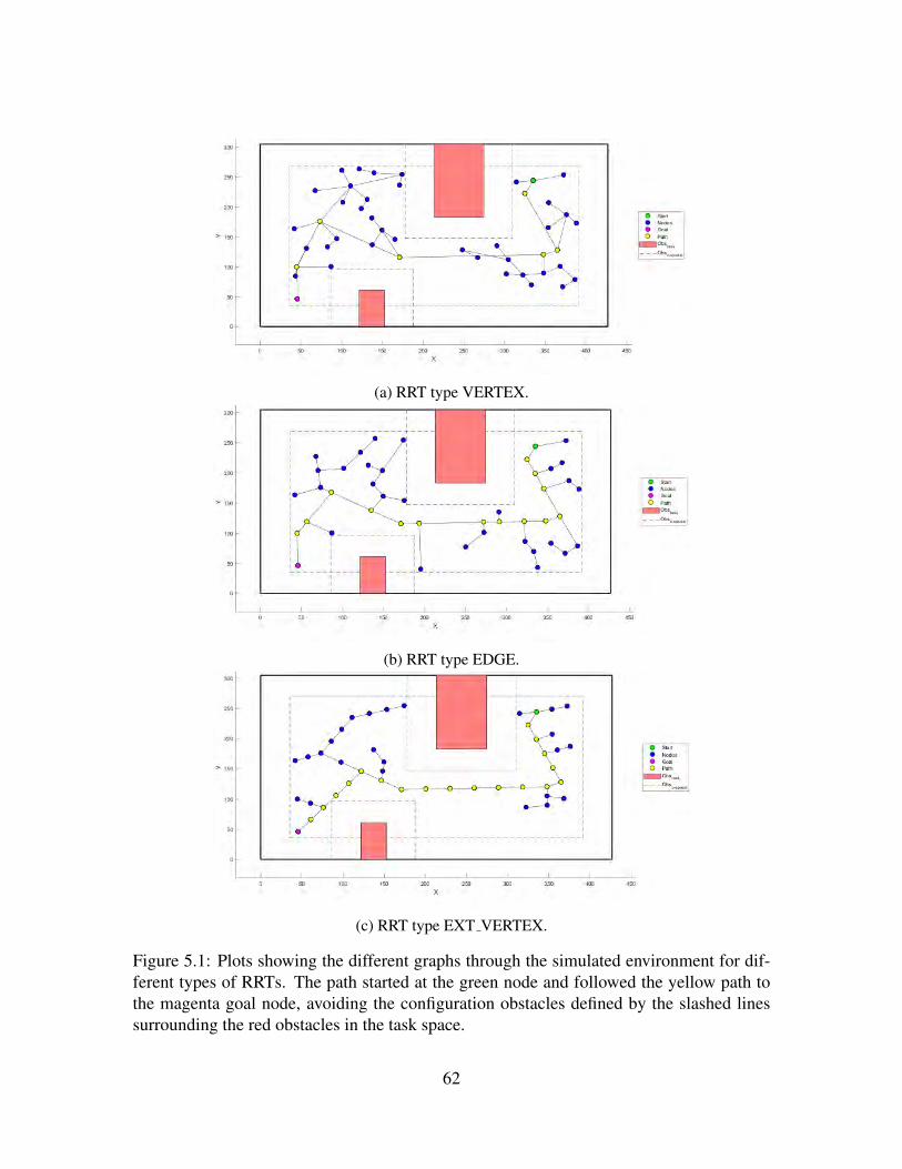
(a) RRT type VERTEX.

(b) RRT type EDGE.

(c) RRT type EXT VERTEX.

Figure 5.1: Plots showing the different graphs through the simulated environment for dif-ferent types of RRTs. The path started at the green node and followed the yellow path tothe magenta goal node, avoiding the configuration obstacles defined by the slashed linessurrounding the red obstacles in the task space.

62

(a) RRT with 20 nodes.

(b) RRT with 100 Nodes.

(c) RRT with 215 Nodes.

Figure 5.2: Plot showing the RRT (type=VERTEX) expanding into an open environment(no obstacles). The green node indicates the start.

63

The cost function g(q) is defined to be the L2-norm traveled along each edge from the

qstart to the q. With this cost function, our heuristic function is admissible, following the

triangle inequality [13]. An admissible heuristic function always underestimates the cost

from any configuration to the goal configuration. Unless the qstart is directly connected to

qgoal , the path will consist of at least two edges. Let q0 = qstart and q2 = qgoal . Let g0,1

be the L2-norm (i.e. cost) from q0 to q1 and g1,2 be the L2-norm (i.e. cost) from q1 to q2.

While q0 and q2 are not connected, let g0,2 be the the cost to travel from q0 directly to q2

(i.e. h(q0) = g0,2). If qstart is directly connected to qgoal then the heuristic value is equal

to the cost, so the admissibility still holds. Therefore, the actual cost to reach the goal is

g0,1 + g1,2 ≤ g0,2 by the triangle inequality. This will guarantee that our A* provides the

optimum path from qstart to qgoal given the tree generated by the RRT. If the RRT was not

successful, then an error is generated and A* is never run.

The output of the A* is the set of action vectors U = {µ1,µ2, . . . µn} to move the

robot from configuration to configuration. For the mobile base, each action vector µ has

two rotations and a translation. The robot must first rotate to face the new configurations,

translate in a straight line to reach the configuration’s x and y position, then finally rotate to

orient itself with the configuration’s θ . The resulting movement of performing U serially

results in superfluous rotations. When traveling from q0 to q1 then on to q2, there is no

reason for the robot to orient itself with θq1 , but rather simply orient itself to face (x,y)q2 .

The set U is passed to a smoothing function Eqn. (5.1) that combines the second rotation

with the first rotation of the following action. The min rot()ϕ) function is the same as that

used in Eqn. (4.7).

64

smooth([ϕi,1 ϕi,2]

T , [ϕi+1,1 ϕi+1,2]T)= (5.1)

{

ϕi,2 = min rot(ϕi,2 +ϕi+1,1) ;

ϕi+1,1 = 0;

}

5.1.3 Testing the RRT and A*

To collect data about the RRT and A* performance, we performed two sets of ex-

periments and the results are shown in the tables Fig. 5.3. For each of these experiments,

20 random seeds were chosen. The RRT/A* algorithm was then run with each of these

seeds and the results (number of nodes, time, path length, etc.) were averaged ( µ ) and the

standard deviations calculated ( σ ).

Figure 5.3: (a) RRT Experiment 1 Results. (b) RRT Experiment 2 Results.

65

Within Experiment 1 and 2, the type of the tree (see above) was changed and the

same 20 seeds were used again. Between Experiment 1 and 2, the Parameters shown in

the first row of the tables were varied and the experiment run again.

From the data, we conclude that the EXT VERTEX is the best type of tree to

run. The time of the RRT execution, while almost doubling that of the VERTEX run-

time, is orders of magnitude less than the EDGE time. The total distance traveled for the

EXT VERTEX is roughly equivalent to the EDGE type, which is an indication of a more

“optimal” path. While the raw Path Rotation is greater than EDGE, the optimized path

rotation is less in both experiments. Another benefit of the EXT VERTEX is that the edges

of the path are, on average, shorter. This can be inferred from the Path Length as measured

in number of nodes. Since small errors are magnified over larger distances, the robot has a

better chance to maintain course. As the data shows, EXT VERTEX performs the best for

the scenario we have used, and is the method used in all of the simulations in the following

sections.

5.1.4 Simulation of Mobile Base RRT

To evaluate the RRT approach, a scenario was designed in which the mobile base

would move from one side of an environment to the other while avoiding obstacles. Fig.5.4

shows the scenario. In the image, the red areas represent the obstacles in the task space. The

thick black border represents the extreme limits of the x-axis and y-axis for this work space

(i.e. the walls of the room). The dashed lines represent the boundaries of the configuration

space obstacles.

While the robot is estimated as a disc, meaning the configuration obstacles formally

should have rounded borders from the Minkowski differences, the obstacles are simply

estimated as the bounding rectangle that encloses the Minkowski difference. This is done

66

Figure 5.4: The configuration space of the mobile base in the scenario presented above

for simplicity in the collision detection. In the scenario, the start position is shown as the

green node and the goal is the pink node.

Preliminarily to implementing the path execution on the robot, animations were

created in MATLAB to visualize the paths as they are created. Fig. 5.5 shows snapshots of

the trees as they are animated, as well as the final RRT with the path generated by the A*

algorithm highlighted.

After the central computer runs the RRT and A* algorithms, it generates *.csv files

of the graph and path. These files are parsed by a MATLAB script to generate the anima-

tions. A different script creates a robot trajectory based on the actions and simulates the

robot as it would follow the path through the environment, as seen in Fig.5.6.

5.2 Path Planning for the Continuum Section

5.2.1 RRT and A*

Using the configuration space for CuRLE that we established in Chapter 4, we ap-

ply the same classical motion planning techniques to map and navigate the continuum

67

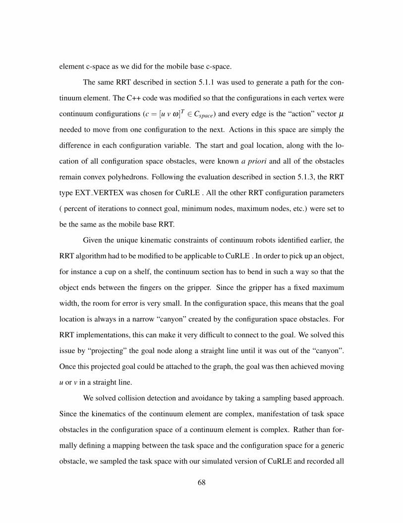
element c-space as we did for the mobile base c-space.

The same RRT described in section 5.1.1 was used to generate a path for the con-

tinuum element. The C++ code was modified so that the configurations in each vertex were

continuum configurations (c = [u v ω]T ∈Cspace) and every edge is the “action” vector µ

needed to move from one configuration to the next. Actions in this space are simply the

difference in each configuration variable. The start and goal location, along with the lo-

cation of all configuration space obstacles, were known a priori and all of the obstacles

remain convex polyhedrons. Following the evaluation described in section 5.1.3, the RRT

type EXT VERTEX was chosen for CuRLE . All the other RRT configuration parameters

( percent of iterations to connect goal, minimum nodes, maximum nodes, etc.) were set to

be the same as the mobile base RRT.

Given the unique kinematic constraints of continuum robots identified earlier, the

RRT algorithm had to be modified to be applicable to CuRLE . In order to pick up an object,

for instance a cup on a shelf, the continuum section has to bend in such a way so that the

object ends between the fingers on the gripper. Since the gripper has a fixed maximum

width, the room for error is very small. In the configuration space, this means that the goal

location is always in a narrow “canyon” created by the configuration space obstacles. For

RRT implementations, this can make it very difficult to connect to the goal. We solved this

issue by “projecting” the goal node along a straight line until it was out of the “canyon”.

Once this projected goal could be attached to the graph, the goal was then achieved moving

u or v in a straight line.

We solved collision detection and avoidance by taking a sampling based approach.

Since the kinematics of the continuum element are complex, manifestation of task space

obstacles in the configuration space of a continuum element is complex. Rather than for-

mally defining a mapping between the task space and the configuration space for a generic

obstacle, we sampled the task space with our simulated version of CuRLE and recorded all

68

the configurations of any collisions, which are detected by sampling along the backbone of

the continuum element and checking for a collision at each point. Fig. 5.8 shows the con-

figuration space manifestation of the task space obstacles shown in Fig. 5.7. This offline

sampling method generates a discrete lookup-table for every possible configuration, sam-

pled at a rate of 0.01 between the minimum and maximum values, for each configuration

variable.

Once the RRT algorithm connected the goal configuration to the graph, we ran the

same A* algorithm as for the base to determine the optimal path. As with the mobile

base, the A* used a heuristic of the L2-norm between a given configuration and the goal

configuration. The cost function was the L2-norm between each node in the current path

from the start node. We also implemented a weighting function to encourage movements

of the continuum arm (u and v) and penalize movements of the revolute joint at the base of

CuRLE (ω). This was done to reduce the overall execution time in the physical hardware.

The algorithm then output the full graph and optimal path to a *.csv file.

5.2.2 Simulation Results

To verify the motion planning algorithms, a simulated environment was created in

MATLAB and a model of CuRLE was developed and added to the simulation. The simu-

lation discussed herein involves a scenario where CuRLE is instructed to pick up a cup off

a shelf by the user (see Fig. 5.7). The task space obstacles were converted to configuration

space obstacles, shown in Fig. 5.8. The start configuration of CuRLE was cstart = [0 0 0]T

and the goal configuration for the example reported herein was cgoal = [−1.76 0 −π/2]T ,

(i.e. the configuration needed to pick up the cup). This goal was determined by using the

interactive GUI developed with the environment to bend the simulated CuRLE until it was

in the correct configuration. Fig. 5.9 shows the interactive GUI with CuRLE in the start

69

configuration.

The output of the RRT/A* was fed into the simulation and Fig. 5.10 shows CuRLE achieving

the goal configuration of grasping the “cup”. For this simulation, we set v = 0 to keep the

configuration space 2D and allow for easy visualization of the nodes from the RRT algo-

rithm.

From the simulation that we ran for both the mobile base RRT/A*, we can predict

that our motion planning algorithms will successfully navigate the configuration space to

guide the robot through the task space. In the proposed scenario, a path for the mobile base

is found rapidly and the simulation shows that the path is collision-free. In addition, we

can conclude that our work to design the RRT to be re-configurable and extensible was a

success. By simply changing the ”state” definition, we generated a collision-free path for

the continuum element through its task space by using its configuration space, which we

verified by our simulation of CuRLE.

70

(a)

(b)

(c)

Figure 5.5: The RRT growth over time.

71

(a)

(b)

(c)

Figure 5.6: A progression of images showing the simulated robot moving through thescenario.

72

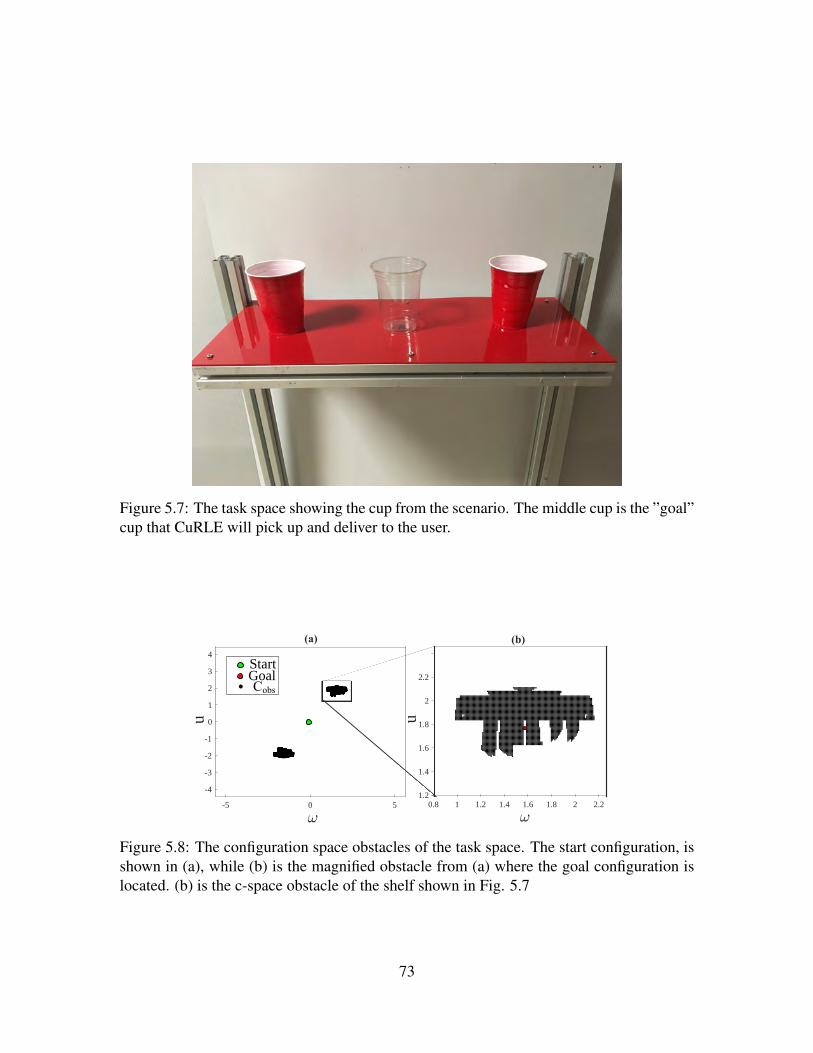
Figure 5.7: The task space showing the cup from the scenario. The middle cup is the ”goal”cup that CuRLE will pick up and deliver to the user.

-5 0 5

-4

-3

-2

-1

0

1

2

3

4

u

StartGoalCobs

0.8 1 1.2 1.4 1.6 1.8 2 2.21.2

1.4

1.6

1.8

2

2.2

u

(a) (b)

Figure 5.8: The configuration space obstacles of the task space. The start configuration, isshown in (a), while (b) is the magnified obstacle from (a) where the goal configuration islocated. (b) is the c-space obstacle of the shelf shown in Fig. 5.7

73

Figure 5.9: The interactive GUI that serves as the front end for simulation environment.

74

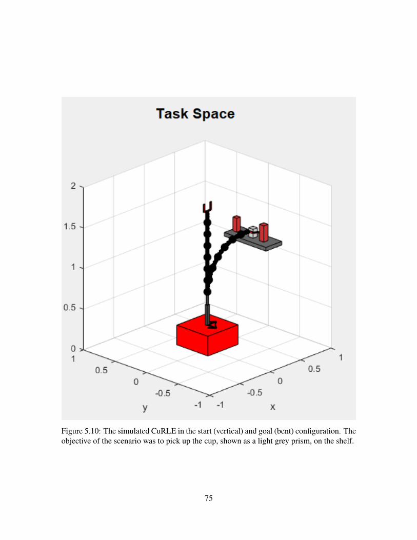
Figure 5.10: The simulated CuRLE in the start (vertical) and goal (bent) configuration. Theobjective of the scenario was to pick up the cup, shown as a light grey prism, on the shelf.

75

Chapter 6

Validation of Motion Planning with

CuRLE Robot Hardware

This Chapter details experimentation done to validate the RRT/A* algorithms de-

veloped in Chapter 5 by implementing them on CuRLE. First we describe the software

running on CuRLE to implement the autonomous motion given a path through the config-

uration spaces. Next we describe an initial experiment to validate the RRT output for the

continuum element on the CuRLE hardware. We then lay out the over-arching in-home sce-

nario that we used to fully validate the work in this thesis regarding the configuration space

and motion planning for a practical hybrid tendon-actuated continuum element/mobile base

operating in free-space. The final sections detail the experiments done and evaluate the re-

sults.

6.1 CuRLE Software Implementation

The software running on the CuRLE hardware is split between the Arduino Due

micro-controller and the Raspberry Pi computer. The Arduino is responsible for interfacing

76

with all of the actuators (motors) and sensors (encoders and tension sensors) in the system.

Implemented in the Arduino IDE (C++), the software controllers running on the Arduino

execute the transitions from the current configuration to the next. The Raspberry Pi serves

as the central computer of CuRLE and is responsible for interfacing with the Arduino.

Primarily running Python scripts, it passes external messages to the Arduino and relays

any response. The Raspberry Pi also stores the current state of the robot, for persistence of

memory when power is lost. Finally, since the Raspberry Pi can be accessed remotely over

the network, we can take direct control of the Pi (and by extension the Arduino) to update

code, execute individual commands, and initiate a debugging session.

6.1.1 Configuration Controller

Much like the controller of the h+lamp (see Chapter 2), the controller(s) running

on the Arduino constantly monitor the current configuration of the robot (i.e. reading the

sensors) and maintain a desired configuration by actuating the motors when the current

configuration strays from the set point (i.e. the error is nonzero). Two PID controllers

generate signals for the motors based on the current error values: one for the mobile base

state and one for the continuum element state.

The controller for the mobile base is fundamentally the same as the one discussed

for the h+lamp. The method for calculating error signals and set points for each drive motor

is as detailed in Chapter 2. The gain values for the PID were tuned differently to work for

the new hardware, but the underlying software is the same.

Because of the unique properties of the continuum element kinematics, the con-

troller for the continuum element fundamentally operates differently from the mobile base

controller. As mentioned in Chapter 3 knowing the length of the tendons is essential for

determining the configuration of the robot. In order to accurately measure the length, the

77

radius of the spool must be known. As such, the controller must also track the radius of

the spool as it changes over time. Because of this, the absolute position of the motor shaft

must always be known and saved.

After initial calibration when CuRLE was first constructed, the current state of the

motor shaft (measured in encoder counts) is saved to a configuration file on the Raspberry

Pi. In addition, the continuum configuration is stored ([u v ω]). Every minute, the Arduino

communicates the state (motor encoder count and the [u v ω] corresponding to those counts)

to Pi and the Pi updates the configuration file. When the system first boots, the Arduino

requests the saved state from the Pi and remains idle until the Pi sends the state. The

controller is able to use the ”zero” state and the current encoder readings to track the radius

of the spools and thereby the lengths of the tendons.

To reach a desired configurations, the same PID controller operates independently

on all four tendons. This controller was tuned until the robot could accurately reach a

desired configuration from its current configuration.

6.1.2 Execution Sequence

To implement the RRT output on CuRLE, the motion planning was done offline on

an external computer. We then transmitted the output files to the Raspberry Pi over the

local network. Rather than have the external computer execute this process automatically,

we found that experimentation was easier if we manually transferred the files. Once the

files were on the Raspberry Pi, we remotely accessed it via SSH and ran an interactive

(via command line) Python program that initiated the Arduino. Once the Arduino received

the saved state and finished its initializing, we executed a command through the Python

program to load the paths (mobile and continuum element) and transmit commands to the

Arduino. Once the Arduino reached the set configuration (i.e. all error signals dropped

78

below a minimum threshold), it sent a message back to the Raspberry Pi to indicate that it

has completed its task. In addition, the Arduino flashed the lamp LEDs to visually commu-

nicate that the set configuration had been reached. The Raspberry Pi, idle until it received

this message from the Arduino, then sent the next configuration in the path. This process

repeated until the goal was reached.

6.2 Validating the Continuum Section Controller

As we did with the h+lamp controller, we first tested the continuum controller’s

ability to ”follow” an RRT path by serially executing the transition from node to node.

Recall from Chapter 5 the simulation experiment done to test the RRT output for the con-

tinuum element. In simulation, we demonstrated the software model of CuRLE bending to

grasp a cup on shelf. We took the same RRT output (shown in Fig. 6.10) and passed this

path to CuRLE. We issued ”grasp” command to grab the cup and then passed CuRLE a

second path from the RRT to lift the cup from the shelf. The results of this experiment are

shown in Fig. 6.1.

6.3 In-Home Scenario

To demonstrate the full functionality of the system, we explored a simple in-home

scenario where the user has asked CuRLE to fetch a cup from shelf, bring the cup into an

adjacent room and set it down on a different shelf, then navigate to its ”docking station”

in another portion of the smaller room. The environment for this scenario is shown in Fig.

6.2. This scenario can be further broken down into three sub-scenarios, each involving

planning for the mobile base and the continuum element. In each sub-scenario, the path(s)

the robot must follow is shown for both the mobile base and the continuum element. We

79

Figure 6.1: (a) The state of CuRLE after ω has aligned with the goal ω . (b) CuRLE hasgrasped the cup. (c) The results of a second path generated by the RRT (shown in Fig.6.11) that guided CuRLE to pick the cup off the shelf.

then show and discuss the results from each experiment.

6.4 Sub-Scenario 1: Simple Base Movement and Grasp-

ing the Cup with Continuum Element

In this sub-scenario, the first set of actions moves CuRLE from the start (Location

1) to the goal (Location 2) to position the robot in front of the shelf. Next, the continuum

element bends to grasp the cup. A ”grasp” command is then issued and CuRLE lifts the

cup from the shelf. Fig. 6.3 shows the path generated by the mobile base RRT, and Fig. 6.4

and 6.5 show the two paths generated by the continuum element RRT.

80

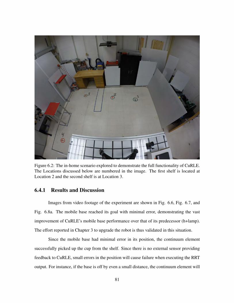
Figure 6.2: The in-home scenario explored to demonstrate the full functionality of CuRLE.The Locations discussed below are numbered in the image. The first shelf is located atLocation 2 and the second shelf is at Location 3.

6.4.1 Results and Discussion

Images from video footage of the experiment are shown in Fig. 6.6, Fig. 6.7, and

Fig. 6.8a. The mobile base reached its goal with minimal error, demonstrating the vast

improvement of CuRLE’s mobile base performance over that of its predecessor (h+lamp).

The effort reported in Chapter 3 to upgrade the robot is thus validated in this situation.

Since the mobile base had minimal error in its position, the continuum element

successfully picked up the cup from the shelf. Since there is no external sensor providing

feedback to CuRLE, small errors in the position will cause failure when executing the RRT

output. For instance, if the base is off by even a small distance, the continuum element will

81

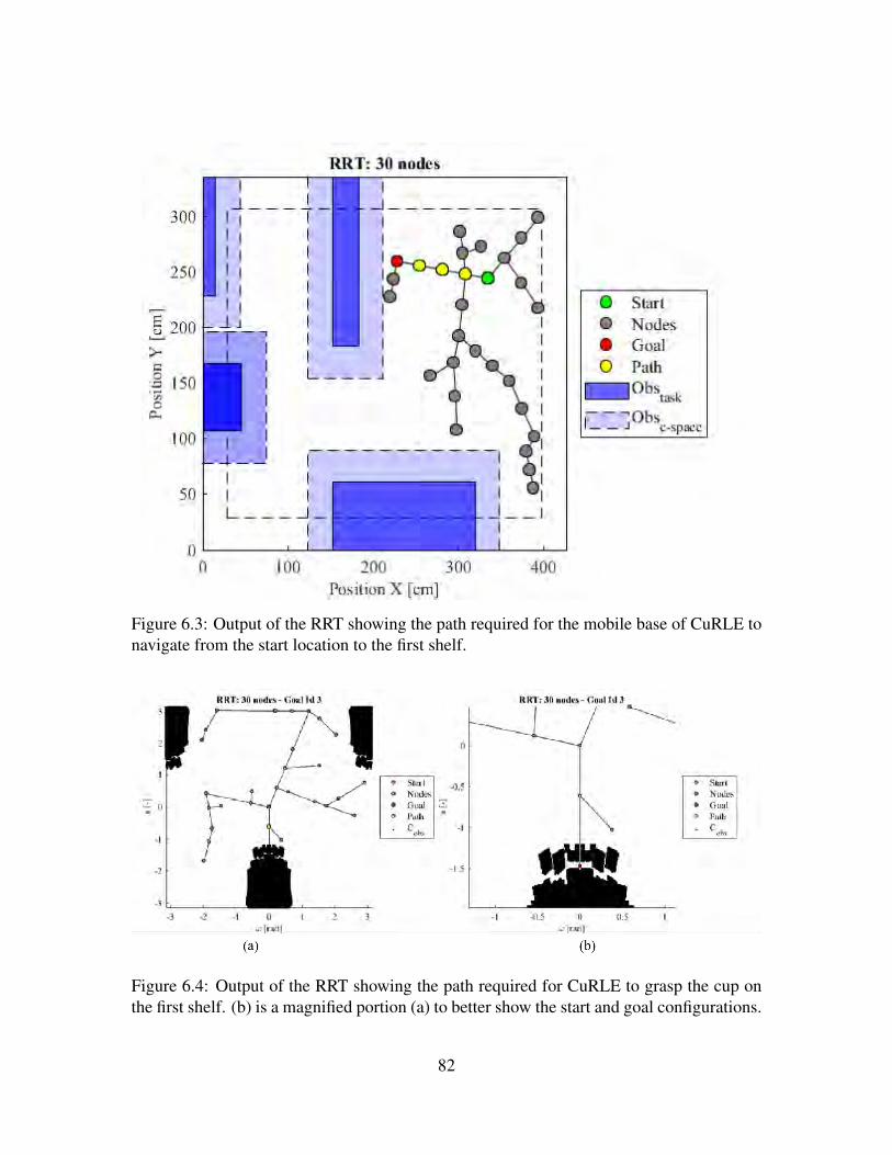
Figure 6.3: Output of the RRT showing the path required for the mobile base of CuRLE tonavigate from the start location to the first shelf.

Figure 6.4: Output of the RRT showing the path required for CuRLE to grasp the cup onthe first shelf. (b) is a magnified portion (a) to better show the start and goal configurations.

82

Figure 6.5: Output of the RRT showing the path required for CuRLE to pick the cup up offthe first shelf. (b) is a magnified portion (a) to better show the start and goal configurations.

miss its goal location. This was seen in initial experimentation and resulted from poor PID

control. By tuning the gains, we reduced the error enough such that the continuum element

was able to grab the cup.

6.5 Sub-Scenario 2: Complex Base Movement and Plac-

ing the Cup with Continuum Element

In this sub-scenario, the first set of actions moves CuRLE from the first shelf (Loca-

tion 2) to the goal (Location 3) to position the robot in front of the shelf. To do this, CuRLE

must travel to the ”second” room, which is on the far side of a ”wall” indicated by the long

vertical obstacle in the center of the task space. Once in the other room, the continuum

element bends to place the cup on the second shelf there. A ”release” command is then

issued and CuRLE bends away from the shelf. Fig. 6.9 shows the path generated by the

mobile base RRT, and Fig. 6.10 and 6.11 show the two paths generated by the continuum

element RRT.

83

6.5.1 Results and Discussion

Images from video footage of the experiment are shown in Fig. 6.8b, Fig. 6.12,

and Fig. 6.13. As with Sub-Scenario 1, the mobile base successfully followed the path and

reached its goal location with minimal error. The continuum element successfully held the

cup during the entire transportation from the ”start” to the ”goal”. Once again, since the

mobile base arrived with small enough error, the continuum element was able to place the

cup on the shelf.

6.6 Sub-Scenario 3: Simultaneous Movement Between Base

and Continuum Element

In this sub-scenario, the first set of actions moves CuRLE from the second shelf

(Location 3) to the goal (Location 4) to position the robot at its ”docking station”. To do

this, CuRLE must navigate the tight space in the ”second” room. While moving through

this room, the continuum element bends to return to its ”home” configuration. This exper-

iment demonstrates the ability for the robot to execute paths from both RRTs in parallel.

Fig. 6.14 shows the path generated by the mobile base RRT, and Fig. 6.15 shows the path

generated by the continuum element RRT.

6.6.1 Results and Discussion

Images from video footage of the experiment are shown in Fig. 6.16 and Fig.

6.17. The final position of the robot is shown in Fig. 6.18. As with the previous two

sub-scenarios, the mobile base successfully navigated from the ”start” configuration to the

”goal”. During this movement, the continuum element also executed its path from the

continuum RRT. We successfully showed the ability of the robot hardware to execute both

84

RRTs in parallel, which was something our simulations had not been able to show.

These experiments show that our motion planning algorithms for both the mobile

base and the continuum element were successfully implemented on the CuRLE robot hard-

ware. As with CuRLE’s predecessor, h+lamp, we saw the robot begin execution of the RRT

output. Unlike h+lamp, CuRLE had the appropriate hardware and well-tuned controllers

that enabled it to successfully complete the tasks. We serially executed multiple RRTs for

the mobile base and continuum element, and we successfully executed the two RRTs in

parallel. Any error generated from the PID control was small enough that the robot still

retrieved and placed the cup on both shelves respectively.

85

Figure 6.6: (a-b) Results from Sub-Scenario 1 showing the execution of the RRT from Fig.6.3 for the mobile base (i.e. CuRLE move from Location 1 to Location 2).

86

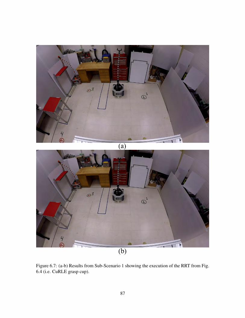
Figure 6.7: (a-b) Results from Sub-Scenario 1 showing the execution of the RRT from Fig.6.4 (i.e. CuRLE grasp cup).

87

Figure 6.8: (a) Results from Sub-Scenario 1 showing the execution of the RRT from Fig.6.5 (i.e. CuRLE lift cup off shelf). (b) Results from Sub-Scenario 2 showing the executionof the RRT from Fig. 6.9.

88

Figure 6.9: Output of the RRT showing the path required for the mobile base of CuRLE tonavigate from the first shelf to the second shelf.

Figure 6.10: Output of the RRT showing the path required for CuRLE to place the cup onthe second shelf.(b) is a magnified portion (a) to better show the start and goal configura-tions.

89

Figure 6.11: Output of the RRT showing the path required for CuRLE to release the cupon the shelf and move away.(b) is a magnified portion (a) to better show the start and goalconfigurations.

90

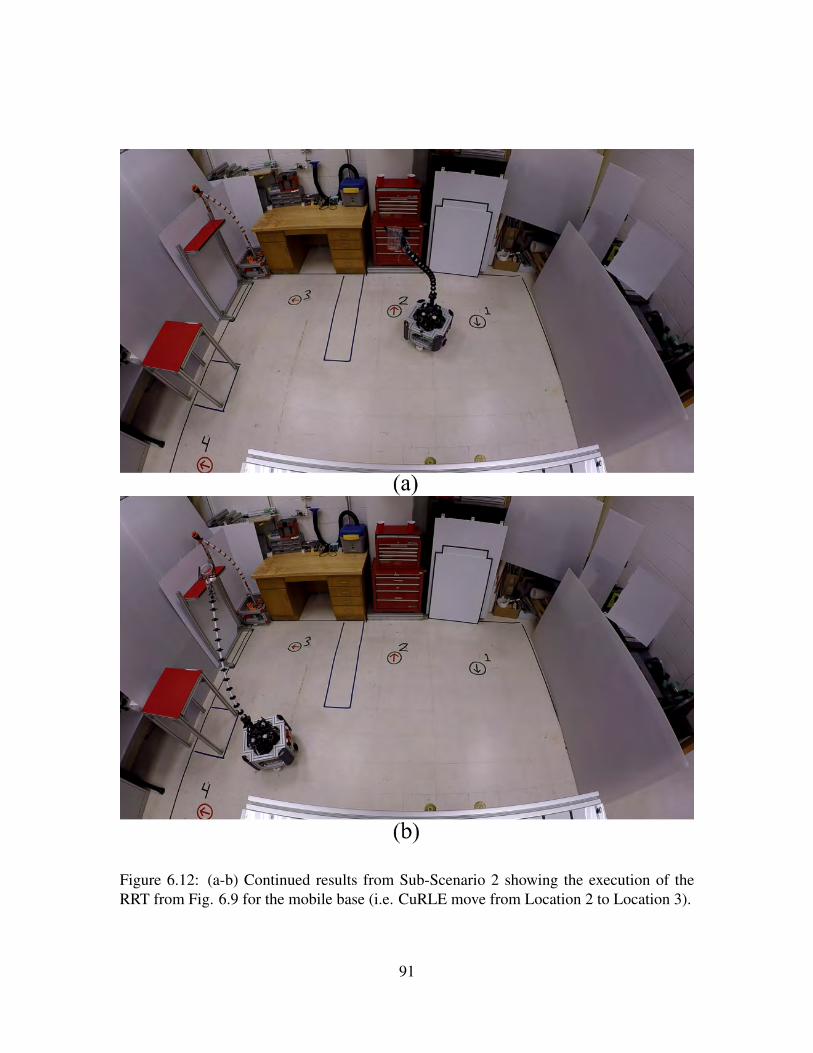
Figure 6.12: (a-b) Continued results from Sub-Scenario 2 showing the execution of theRRT from Fig. 6.9 for the mobile base (i.e. CuRLE move from Location 2 to Location 3).

91

Figure 6.13: (a-b) Results from Sub-Scenario 2 showing the execution of the RRT fromFig. 6.10 (i.e. CuRLE release the cup).

92

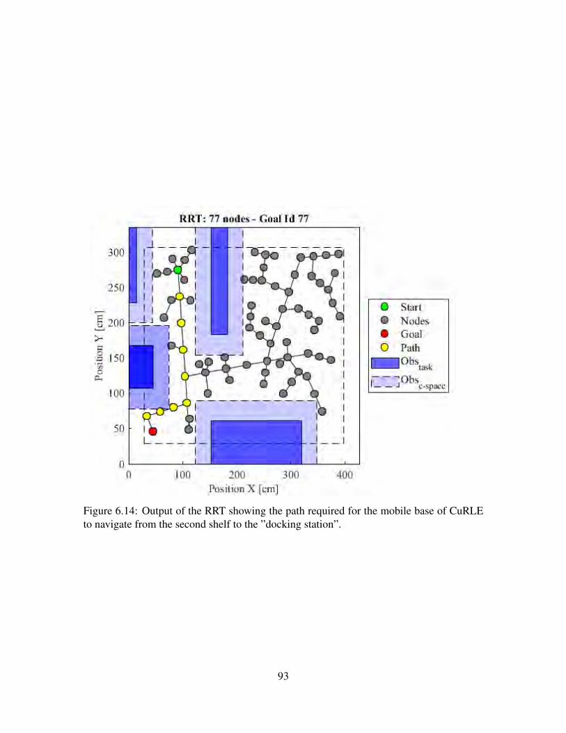
Figure 6.14: Output of the RRT showing the path required for the mobile base of CuRLEto navigate from the second shelf to the ”docking station”.

93

Figure 6.15: Output of the RRT showing the path required for CuRLE to return to its”home” state ([u = 0,v = 0,w = 0])

94

Figure 6.16: (a-b) Results from Sub-Scenario 3 showing the execution of the RRT fromFig. 6.14 for the mobile base executing in parallel with the output of the RRT from Fig.6.15 (i.e. CuRLE return to ”home” state while moving from Location 3 to Location 4).

95

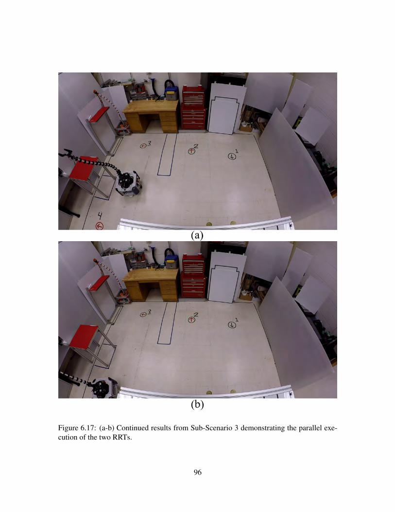
Figure 6.17: (a-b) Continued results from Sub-Scenario 3 demonstrating the parallel exe-cution of the two RRTs.

96

Figure 6.18: Final results of entire experimentation showing the small amount of error inthe final position of the mobile base.

97

Chapter 7

Conclusions and Suggestions for Future

Research

7.1 Conclusions

In Chapter 2, we detailed our first attempt at realizing our continuum robotic mo-

bile lamp as an autonomous system. We recounted the wider history of the home+ effort

and described the motivation for the work later conducted and described in Chapters 4 &

5. In evaluating the level of control the user should have when interacting with the home+

suite of robots, a spectrum arises with tele-operation at one end and full autonomy at the

other. We described work done to implement tele-operation (i.e. the user is in full con-

trol of the robot) via different hardware controllers. To move towards full autonomy in

the robot, we implemented the RRT/A* algorithms, detailed in Chapter 5, for the mobile

base of the h+lamp. The robot successfully received and tried to execute the path through

the in-home environment, but was partially unsuccessful due to hardware limitations and

controller shortcomings.

In Chapter 3, we detailed the upgrades that we made to the original home+ robot

98

hardware (i.e. h+lamp) to correct the issues seen in the experiments in Chapter 2. In addi-

tion, we expanded the robot’s hardware and software, renaming it CuRLE in the process,

to include the capacity to execute the output from motion planning algorithms, developed

in Chapter 5, for the continuum element.

In Chapter 4, we defined the configuration space of a generic single-section exten-

sible continuum element. To develop motion planning algorithms to control our CuRLE

robot hardware, we first needed to understand and visualize the configuration space of the

robot. While the c-space of a mobile robot is well understood, there has been no formal

definition for the configuration space of a continuum element. This thesis presents the first

definition of the configuration space in the general case, and then examines how the phys-

ical build of our continuum section introduces boundaries in the space. By understanding

the unique features of continuum elements and how these features affect the c-space, we

created a foundation to apply classical motion planning algorithms for a practical tendon-

actuated continuum element. Further, we showed how we can separate the configuration

space of the continuum element from that of the mobile base, and thereby characterize the

full, complex configuration space of a hybrid continuum, rigid-link, mobile robot in terms

of two simple 3D spaces.

In Chapter 5, we used the configuration spaces laid out in Chapter 4 to implement

RRT/A* algorithms to plan collision-free paths through the task space of our CuRLE robot.

We chose RRTs since their ability to be an anytime-approach fits well with the dynamic

nature of CuRLE’s operating environment. Given a start and goal configuration, as well as

the location of all obstacles, our motion planning algorithms successfully found a collision-

free path for both the mobile base and the continuum element. This is the first time that

an RRT approach has been applied to a practical tendon-actuated continuum element. The

hybrid nature of our CuRLE robot lends novelty to the motion planning of the mobile base,

even though RRTs have widely been used to provide collision-free paths. We validated our

99

approach by creating software models of our robot and running simulations of practical

in-home scenarios, all of which were successful.

In Chapter 6, we implement the RRT/A* algorithm for the first time on a practi-

cal robot featuring a tendon-actuated continuum element. Experiments described in this

Chapter showed the robot successfully executing a path through the continuum task space.

We integrated the controller from Chapter 2 with the software controlling the continuum

element to create a cohesive solution that was able to simultaneously navigate both config-

uration spaces of the CuRLE robot hardware. Experiments reported in this Chapter show

CuRLE moving through the in-home scenario to successfully complete a complex series of

tasks, guided by the RRT/A* algorithms. The robot demonstrated its potential to provide

in-home care and assist with aging-in-place.

7.2 Future Work

7.2.1 Migrate CuRLE to a Fully Independent System

While the CuRLE hardware was able to autonomously follow the path generated by

the motion planning software, the central computer was still required to run the RRT/A*

and communicate the path to the robot. Since CuRLE already has the Raspberry Pi on-

board to handle its wireless communication and interface with the Arduino Due, we rec-

ommend that the motion planning code be ported over to the Pi. The code already runs in

C++ and uses the Boost Graph library, which is platform independent. If the Raspberry Pi

handles all of the path planning, then the robot will no longer have to rely on another com-

puter to handle the motion planning. This will help streamline the development process

and take the next step towards CuRLE being an autonomous, stand-alone unit. In addition,

we envision several added features that would allow users and developers to interact more

100

directly with Raspberry Pi without relying on a SSH or Virtual Desktop connection. Hav-

ing an LCD display and user input devices would facilitate future development and provide

a method for future users to engage with the robot. In addition, having an audio system

would allow CuRLE to provide added feedback to the user beyond the visual feedback of

the LEDs described in Chapter 6. These relatively simple upgrades would allow future

developers easier avenues for new system features and would provide users with a richer,

more fulfilling experience.

7.2.2 Further Simulation Software Development

In addition to the upgrades to make CuRLE a stand-alone unit, we recommend fur-

ther development of the software model and simulation environment of CuRLE. Combining

the interactive GUI described in Chapter 5 for the continuum arm with the simulation code

for the mobile base also detailed in that Chapter would allow future researchers to perform

more comprehensive studies and experiments with the motion planning algorithms. In this

thesis, we described the justification we used to separate the configurations spaces of the

continuum element and the mobile base, and we were able to experiment in simulation with

each individually, but we were unable to do so with both spaces in parallel. Having the ca-

pacities to run such studies would be useful in validating the motion planning output before

implementing it on the hardware. In addition, while we studied different configurations of

the RRT, more research can be done in this area, particularly in regards to optimization of

the RRT using the RRT* algorithm. Rather than simply find a path to the goal, the mo-

tion planning can be used to find the optimal path. Since the robot will be interacting with

humans to accomplish tasks, it will be important for it to execute relatively quickly. Since

the CuRLE hardware and controllers may continue to present limitations, the more com-

prehensive simulation software that we are proposing will allow these new experiments to

101

be executed and tested before transporting them to the hardware.

7.2.3 Remove Restrictions on Degrees of Freedom

In this work, we restricted several of the DoF of the robot, and in future develop-

ment, we intend these restrictions to be lifted. One of the advantages of the limited DoF was

that we were able to visualize the RRT output in the configuration space of the robot. While

removing the restrictions will necessarily make visualization impossible, advancements in

the simulation software, as we have suggested, will allow us to test the full, unlocked ca-

pacity of the robot. CuRLE will be able to function with all of its DoF and we can use the

simulations to verify the motion planning before executing it on the hardware.

7.2.4 Hardware Upgrades

Many of the existing hardware limitations would be eliminated by making upgrades

to the CuRLE robot. First, the stiffness of the springs in the tension sensors should be

increased. Given the magnitudes of the forces required in the tendons to realize the robot

kinematics, the linear spring-loaded potentiometers saturated their tension readings without

being able to accurately give a measurement of the tension in the tendon. While this allowed

the controller to keep ”slack” out of the tendon by keeping the tension above a threshold

close to the saturation value, it prevented the controller from keeping the tension balanced

between opposing tendons. As such, the tension feedback controller was only marginally

useful, and largely left unused during experimentation.

In addition to upgrading the tension sensors, the spool mechanism for winding the

tendons around the motor shaft should be upgraded. As we previously mentioned, the

spools are integral for accurately tracking the length of the tendons, which is crucial for

the kinematics and control of the robot. The current hardware design does not perfectly

102

align the spool with the tendon as it travels up the backbone, meaning that there is a slight

probability of the tendon slipping off of the spool. This occurred multiple times during

testing, and were it not for the tension sensors, would have ruined controller’s ability to

estimate the tendon length. In addition to routing the tendons more accurately, a new,

more reliable, method should be developed to track the tendon length. This issue could be

potentially solved in software by creating a tracking model to account for dynamic noise

(e.g. slipping) in the tendon winding, or it could solved with a more sophisticated hardware

design. We envision a collection of passive spools that guarantee tendon alignment, with

an optical encoder attached to one of the spools to measure the change in tendon length

without having the current issue of a varying spool radius.

The final hardware upgrade that we propose for future research is to develop a new

material to replace the PEX backbone. Over time, the material properties of the current

backbone cause it to deform as it bends, especially when CuRLE bends to its extremes.

In fact, even the constant strain of gravity causes the material to deform, which eliminates

constant curvature. As the backbone strays from constant curvature, a foundational as-

sumption for the kinematic model, the control of the robot degrades. Since we assume

constant curvature, the actions needed to reach a configuration will evolve the robot into a

shape that we do not model, which causes errors in the navigation. We recommend devel-

opment or selection of a synthetic material (e.g. polyurethane, silicon rubber, etc.) to create

a new backbone for CuRLE. The material must be elastic enough to return to its original

shape after bending but also rigid enough to support its own weight (with the help of the

tendons) without collapsing under gravity.

103

7.2.5 Integrating with a Sensing Network

Since CuRLE is the realization of a key aspect of the ”fully autonomous” end of the

user control spectrum, integrating the robot with sensing technology will be vital for future

development. In this thesis, the ”sensing problem” was solved by assuming knowledge of

the locations of the goal configurations and the exact layout of the environments a priori.

For the robotic lamp to claim full autonomy, it must be able to process user commands

(e.g. voice recognition system) and sense the environment (e.g. vision system) to avoid

obstacles and locate its goal. To accomplish this, we envision at a least two vision systems:

a ”global” system that acts as a Moniter of the Operating Environment (MOE) that is

mounted as an ”eye-in-sky” and detects the environment and communicates with CuRLE.

The second vision system is local, mounted at the end-effector of CuRLE. This would be

primarily used with locating objects to pick up/place. In addition to these vision systems,

we could imagine other sensors in the home as part of the ”smart home” societal trend.

Whether it be other members of home+, like the Linearly Actuated Robotic End-table

Element (LAREE), or other devices that been integrated with ”smart” technology, we hope

that CuRLE will be fully integrated in the home to provide care and assist with aging-in-

place.

104

Appendices

105

Appendix A CuRLE Robot Software: Arduino

1 # i n c l u d e <SPI . h>

2 # i n c l u d e <pwm lib . h>

3 # i n c l u d e ” aux . h ”

4

5 / / Continuum S t a t e V a r i a b l e s

6 c o n s t f l o a t s = 1 . 0 3 ;

7 c o n s t f l o a t d = 0 . 0 2 2 ;

8

9 i n t 3 2 t eCount [ 5 ] ;

10 i n t 3 2 t p revCn t [ ] = { 0 , 0 , 0 , 0 , 0 , 0 } ;

11 c o n s t i n t 3 2 t eCountZero [ ] = { 77514 , 72058 , 70443 , 73889 , 0 } ;

12 f l o a t spoo ledLen [ 4 ] ;

13 f l o a t K tendon [ ] = { 0 . 1 5 , 0 . 0 0 1 , 0 . 0 2 , 0 . 1 5 , 0 . 0 0 1 , 0 . 0 2 } ;

14

15 f l o a t u = 0 ;

16 f l o a t v = 0 ;

17 f l o a t w = 0 ;

18

19 f l o a t u s e t = 0 ;

20 f l o a t v s e t = 0 ;

21 f l o a t w s e t = 0 ;

22

23 boo l d e b u g P r i n t = f a l s e ;

24 boo l ESTOP = t r u e ;

25 boo l i n i t i a l i z e d = f a l s e ;

26 boo l i d l e = t r u e ;

27

28 / / Mobile Base

29 f l o a t mu [ 3 ] ;

106

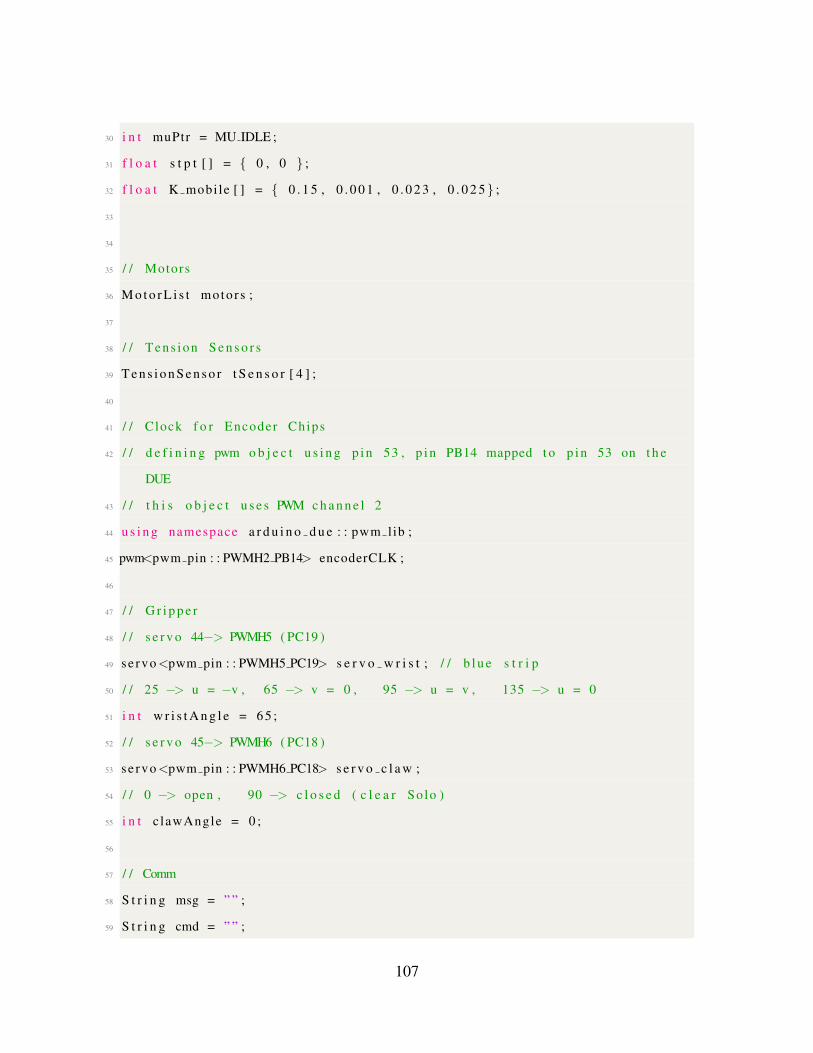
30 i n t muPtr = MU IDLE ;

31 f l o a t s t p t [ ] = { 0 , 0 } ;

32 f l o a t K mobi le [ ] = { 0 . 1 5 , 0 . 0 0 1 , 0 . 0 2 3 , 0 . 0 2 5} ;

33

34

35 / / Motors

36 M o t o r L i s t moto rs ;

37

38 / / Tens ion S e n s o r s

39 T e n s i o n S e n s o r t S e n s o r [ 4 ] ;

40

41 / / Clock f o r Encoder Chips

42 / / d e f i n i n g pwm o b j e c t u s i n g p i n 53 , p i n PB14 mapped t o p i n 53 on t h e

DUE

43 / / t h i s o b j e c t u s e s PWM c h a n n e l 2

44 u s i n g namespace a r d u i n o d u e : : pwm lib ;

45 pwm<pwm pin : : PWMH2 PB14> encoderCLK ;

46

47 / / G r i p p e r

48 / / s e r v o 44−> PWMH5 ( PC19 )

49 se rvo<pwm pin : : PWMH5 PC19> s e r v o w r i s t ; / / b l u e s t r i p

50 / / 25 −> u = −v , 65 −> v = 0 , 95 −> u = v , 135 −> u = 0

51 i n t w r i s t A n g l e = 6 5 ;

52 / / s e r v o 45−> PWMH6 ( PC18 )

53 se rvo<pwm pin : : PWMH6 PC18> s e r v o c l a w ;

54 / / 0 −> open , 90 −> c l o s e d ( c l e a r Solo )

55 i n t c lawAngle = 0 ;

56

57 / / Comm

58 S t r i n g msg = ” ” ;

59 S t r i n g cmd = ” ” ;

107

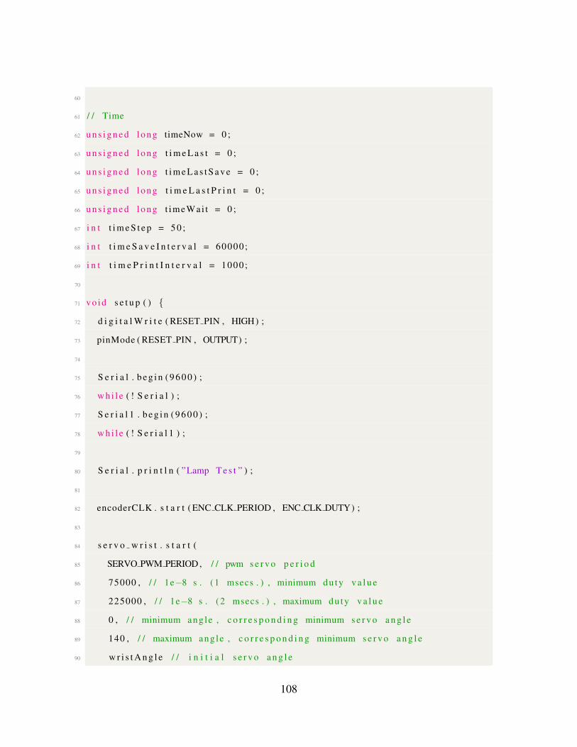
60

61 / / Time

62 u n s i g n e d long timeNow = 0 ;

63 u n s i g n e d long t i m e L a s t = 0 ;

64 u n s i g n e d long t i m e L a s t S a v e = 0 ;

65 u n s i g n e d long t i m e L a s t P r i n t = 0 ;

66 u n s i g n e d long t imeWai t = 0 ;

67 i n t t i m e S t e p = 5 0 ;

68 i n t t i m e S a v e I n t e r v a l = 60000 ;

69 i n t t i m e P r i n t I n t e r v a l = 1000 ;

70

71 vo id s e t u p ( ) {

72 d i g i t a l W r i t e ( RESET PIN , HIGH) ;

73 pinMode ( RESET PIN , OUTPUT) ;

74

75 S e r i a l . b e g i n ( 9 6 0 0 ) ;

76 w h i l e ( ! S e r i a l ) ;

77 S e r i a l 1 . b e g i n ( 9 6 0 0 ) ;

78 w h i l e ( ! S e r i a l 1 ) ;

79

80 S e r i a l . p r i n t l n ( ”Lamp T e s t ” ) ;

81

82 encoderCLK . s t a r t ( ENC CLK PERIOD , ENC CLK DUTY) ;

83

84 s e r v o w r i s t . s t a r t (

85 SERVO PWM PERIOD , / / pwm s e r v o p e r i o d

86 75000 , / / 1e−8 s . (1 msecs . ) , minimum du ty v a l u e

87 225000 , / / 1e−8 s . (2 msecs . ) , maximum du ty v a l u e

88 0 , / / minimum ang le , c o r r e s p o n d i n g minimum s e r v o a n g l e

89 140 , / / maximum ang le , c o r r e s p o n d i n g minimum s e r v o a n g l e

90 w r i s t A n g l e / / i n i t i a l s e r v o a n g l e

108

91 ) ;

92 s e r v o c l a w . s t a r t (

93 SERVO PWM PERIOD , / / pwm s e r v o p e r i o d

94 75000 , / / 1e−8 s . (1 msecs . ) , minimum du ty v a l u e

95 225000 , / / 1e−8 s . (2 msecs . ) , maximum du ty v a l u e

96 0 , / / minimum ang le , c o r r e s p o n d i n g minimum s e r v o a n g l e

97 140 , / / maximum ang le , c o r r e s p o n d i n g minimum s e r v o a n g l e

98 clawAngle / / i n i t i a l s e r v o a n g l e

99 ) ;

100

101 / / S w i t c h e s

102 pinMode (SW LED, OUTPUT) ;

103 aux : : s e t s w i t c h (SW LED, OFF ) ;

104

105 pinMode (SW DRV, OUTPUT) ;

106 aux : : s e t s w i t c h (SW DRV, OFF) ;

107

108 / / Have t o s t a r t SPI b e f o r e i n i t i a l i z i n g motors ( f o r t h e e n c o d e r s )

109 SPI . b e g i n ( ) ;

110 motors . i n i t ( ) ;

111

112 / / I n i t i a l i z e t h e t e n s i o n s e n s o r s ( a n a l o g i n p u t s )

113 a n a l o g R e a d R e s o l u t i o n ( 1 2 ) ;

114 t S e n s o r [ 0 ] . i n i t ( T SENSOR1 ) ;

115 t S e n s o r [ 1 ] . i n i t ( T SENSOR2 ) ;

116 t S e n s o r [ 2 ] . i n i t ( T SENSOR3 ) ;

117 t S e n s o r [ 3 ] . i n i t ( T SENSOR4 ) ;

118

119 / / s t a t u s v a r i a b l e s

120 ESTOP = t r u e ;

121 i n i t i a l i z e d = f a l s e ;

109

122

123 / / r e q u e s t t h e s t a t e d a t a from t h e R a s p b e r r y P i

124 sendRasPiMsg ( RPI LOAD ) ;

125 }

126

127 vo id loop ( ) {

128 f l o a t l e n [ 4 ] , d e l t a L e n [ 4 ] ;

129 f l o a t s e t [ 4 ] ; / / d r i v e motors use s t p t [ ] , which i s g l o b a l

130 s t a t i c i n t 3 2 t e r r L a s t [ ] = { 0 , 0 , 0 , 0 , 0 , 0} ;

131

132 i n t t e n s i o n E r r ;

133 f l o a t t e n s i o n K ;

134

135 s t a t i c RunningSum<i n t 3 2 t > errSum [ 6 ] ;

136 s t a t i c bo o l once = t r u e ;

137 i n t 3 2 t e r r [ 6 ] ;

138 i n t 3 2 t c n t [ 6 ] , d e l t a C [ 6 ] ;

139 i n t CPR , i , k ;

140 f l o a t pwm [ 6 ] ;

141 c o n s t f l o a t TENDON PWM SAT = 1 0 0 . 0 ;

142 c o n s t f l o a t DRIVE PWM SAT = 7 5 ;

143 c o n s t i n t 3 2 t TENDON ERR THRESH = 4 0 ;

144 c o n s t i n t 3 2 t DRIVE ERR THRESH = 6 0 ;

145 c o n s t i n t TENSION THRESH = 4000 ;

146 boo l c o m p l e t e [ ] = { f a l s e , f a l s e , f a l s e , f a l s e , f a l s e , f a l s e } ;

147 s t a t i c i n t comple t eCn t = 0 ;

148

149 i f ( once ) {

150 f o r ( i n t i = T MOTOR1 ; i <= D MOTOR2; ++ i ) {

151 errSum [ i ] . i n i t ( 1 0 ) ;

152 }

110

153 once = f a l s e ;

154 }

155

156 timeNow = m i l l i s ( ) ;

157

158 i f ( ! i n i t i a l i z e d ) {

159 i f ( timeNow − t i m e L a s t > 1000) {

160 / / aux : : t o g g l e (SW LED) ;

161 t i m e L a s t = timeNow ;

162 }

163 }

164 e l s e

165 {

166

167

168

169 / / s h o u l d o c c u r e v e r y 50ms

170 i f ( ( timeNow−t i m e L a s t ) >= t i m e S t e p ) {

171 / / K i n e m a t i c s

172 / / g e t l e n g t h s from t h e c u r r e n t s t a t e

173 l e n [T MOTOR1] = s − ( v*d ) ;

174 l e n [T MOTOR3] = s + ( v*d ) ;

175 l e n [T MOTOR2] = s + ( u*d ) ;

176 l e n [T MOTOR4] = s − ( u*d ) ;

177

178 / / u p d a t e c u r r e n t s t a t e [ u , v , w]

179 / / g e t t h e c u r r e n t c o u n t s

180 f o r ( i = T MOTOR1 ; i <= T MOTOR4 ; ++ i ) {

181 c n t [ i ] = eCount [ i ] + motors [ i ] . g e t C o u n t ( ) ;

182 d e l t a C [ i ] = c n t [ i ] − prevCn t [ i ] ;

183 / / t h i s i s r e a l l y t h e d e l t a l e n g t h

111

184 d e l t a L e n [ i ] = aux : : l eng t hOnSp oo l ( moto rs [ i ] . CPR ( ) , p r evCn t [ i ] ) −

aux : : l eng thOnSp oo l ( moto rs [ i ] . CPR ( ) , c n t [ i ] ) ;

185 l e n [ i ] += d e l t a L e n [ i ] ;

186 }

187

188 / / g e t c o u n t s from t h e d r i v e motors

189 f o r ( i = D MOTOR1; i <= D MOTOR2; ++ i ) {

190 c n t [ i ] = motors [ i ] . ge t C o u n t ( ) ;

191 }

192

193

194 / / S e t p o i n t s f o r t e nd on motors

195 s e t [T MOTOR1] = s − ( v s e t *d ) ;

196 s e t [T MOTOR3] = s + ( v s e t *d ) ;

197 s e t [T MOTOR2] = s + ( u s e t *d ) ;

198 s e t [T MOTOR4] = s − ( u s e t *d ) ;

199

200

201

202 / / c a l c u l a t e e r r o r s

203 f o r ( i = T MOTOR1 ; i <= T MOTOR4 ; ++ i ) {

204 CPR = motors [ i ] . CPR ( ) ;

205

206 / / c a l c u l a t e t e n s i o n e r r o r ( n o t used . . . )

207 t e n s i o n E r r = t S e n s o r [ i ] . r e a d ( )−TENSION THRESH ;

208 t e n s i o n E r r = ( t e n s i o n E r r > 0) ? 0 : t e n s i o n E r r ;

209

210 e r r [ i ] = aux : : d e l t a L e n g t h T o S e t C o u n t (CPR , c n t [ i ] , ( s e t [ i ] − l e n [ i

] ) ) − c n t [ i ] ;

211

212 k = 0 ;

112

213 pwm[ i ] = ( e r r [ i ]* K tendon [0+ k ] ) + ( e r r [ i ] − e r r L a s t [ i ] ) / (

s t a t i c c a s t <f l o a t >(timeNow−t i m e L a s t ) / 1 0 0 0 . 0 ) * K tendon [1+ k ] + errSum [

i ] . add ( e r r [ i ] ) * K tendon [2+ k ] ;

214 pwm[ i ] = (pwm[ i ] < 0) ? max (pwm[ i ] ,−TENDON PWM SAT) : min (pwm[ i ] ,

TENDON PWM SAT) ;

215 }

216

217 d e l t a C [D MOTOR1] = ( c n t [D MOTOR1]−prevCn t [D MOTOR1 ] )−( c n t [D MOTOR2]−

prevCn t [D MOTOR2 ] ) ;

218 d e l t a C [D MOTOR2] = ( c n t [D MOTOR2]−prevCn t [D MOTOR2 ] )−( c n t [D MOTOR1]−

prevCn t [D MOTOR1 ] ) ;

219 f o r ( i = D MOTOR1; i <= D MOTOR2; ++ i ) {

220 e r r [ i ] = s t p t [ i−D MOTOR1] − c n t [ i ] ;

221 / / PID c o n t r o l and v e l o c i t y c o n t r o l ( i . e . t r y t o keep them a t t h e

same speed )

222 pwm[ i ] = ( e r r [ i ]* K mobi le [ 0 ] ) + ( e r r [ i ] − e r r L a s t [ i ] ) / ( s t a t i c c a s t

<f l o a t >(timeNow−t i m e L a s t ) / 1 0 0 0 . 0 ) * K mobi le [ 1 ] + errSum [ i ] . add ( e r r [ i

] ) * K mobi le [ 2 ] − d e l t a C [ i ]* K mobi le [ 3 ] ;

223 pwm[ i ] = (pwm[ i ] < 0) ? max (pwm[ i ] ,−DRIVE PWM SAT) : min (pwm[ i ] ,

DRIVE PWM SAT) ;

224 }

225

226 i f ( timeNow − t i m e L a s t P r i n t > t i m e P r i n t I n t e r v a l ) {

227 i f ( d e b u g P r i n t ) {

228 / / S e r i a l . p r i n t l n ( ” s p l : [”+ S t r i n g ( spoo ledLen [ 0 ] , 4 ) +” ,”+ S t r i n g (

spoo ledLen [ 1 ] , 4 ) +” ,”+ S t r i n g ( spoo ledLen [ 2 ] , 4 ) +” ,”+ S t r i n g ( spoo ledLen

[ 3 ] , 4 ) + ” ] ” ) ;

229 / / S e r i a l . p r i n t l n ( ” dCt : [”+ S t r i n g ( d e l t a C [ 0 ] ) +” ,”+ S t r i n g ( d e l t a C

[ 1 ] ) +” ,”+ S t r i n g ( d e l t a C [ 2 ] ) +” ,”+ S t r i n g ( d e l t a C [ 3 ] ) + ” ] ” ) ;

230 S e r i a l . p r i n t l n ( ” dCt : [ ”+ S t r i n g ( d e l t a C [ 4 ] ) +” , ”+ S t r i n g ( d e l t a C [ 5 ] ) +

” ] ” ) ;

113

231 / / S e r i a l . p r i n t l n ( ” dLn : [”+ S t r i n g ( d e l t a L e n [ 0 ] , 4 ) +” ,”+ S t r i n g (

d e l t a L e n [ 1 ] , 4 ) +” ,”+ S t r i n g ( d e l t a L e n [ 2 ] , 4 ) +” ,”+ S t r i n g ( d e l t a L e n [ 3 ] , 4 )

+ ” ] ” ) ;

232 / / S e r i a l . p r i n t l n ( ” l e n : [”+ S t r i n g ( l e n [ 0 ] , 4 ) +” ,”+ S t r i n g ( l e n [ 1 ] , 4 )

+” ,”+ S t r i n g ( l e n [ 2 ] , 4 ) +” ,”+ S t r i n g ( l e n [ 3 ] , 4 ) + ” ] ” ) ;

233 / / S e r i a l . p r i n t l n ( ” s e t : [”+ S t r i n g ( s e t [ 0 ] , 4 ) +” ,”+ S t r i n g ( s e t [ 1 ] , 4 )

+” ,”+ S t r i n g ( s e t [ 2 ] , 4 ) +” ,”+ S t r i n g ( s e t [ 3 ] , 4 ) + ” ] ” ) ;

234 S e r i a l . p r i n t l n ( ” s t p : [ ”+ S t r i n g ( s t p t [ 0 ] ) +” , ”+ S t r i n g ( s t p t [ 1 ] ) +” ] ” )

;

235 S e r i a l . p r i n t l n ( ” e r r : [ ”+ S t r i n g ( e r r [ 0 ] ) +” , ”+ S t r i n g ( e r r [ 1 ] ) +” , ”+

S t r i n g ( e r r [ 2 ] ) +” , ”+ S t r i n g ( e r r [ 3 ] ) +” , ”+ S t r i n g ( e r r [ 4 ] ) +” , ”+ S t r i n g ( e r r

[ 5 ] ) +” ] ” ) ;

236 / / S e r i a l . p r i n t l n ( ” errSum : [”+ S t r i n g ( errSum [ 0 ] . sum ( ) ) +” ,”+ S t r i n g (

errSum [ 1 ] . sum ( ) ) +” ,”+ S t r i n g ( errSum [ 2 ] . sum ( ) ) +” ,”+ S t r i n g ( errSum [ 3 ] .

sum ( ) ) + ” ] ” ) ;

237 S e r i a l . p r i n t l n ( ”pwm: [ ”+ S t r i n g (pwm[ 0 ] , 4 ) +” , ”+ S t r i n g (pwm[ 1 ] , 4 ) +” ,

”+ S t r i n g (pwm[ 2 ] , 4 ) +” , ”+ S t r i n g (pwm[ 3 ] , 4 ) +” , ”+ S t r i n g (pwm[ 4 ] , 4 ) +” , ”+

S t r i n g (pwm[ 5 ] , 4 ) +” ] ” ) ;

238 / / S e r i a l . p r i n t l n ( ” mCt : [”+ S t r i n g ( motors [ 0 ] . g e t C o u n t ( ) ) +” ,”+

S t r i n g ( motor s [ 1 ] . g e t C o un t ( ) ) +” ,”+ S t r i n g ( motors [ 2 ] . g e t C o u n t ( ) ) +” ,”+

S t r i n g ( motor s [ 3 ] . g e t C o un t ( ) ) + ” ] ” ) ;

239 S e r i a l . p r i n t l n ( ”mCt : [ ”+ S t r i n g ( motor s [ 4 ] . g e t C o u n t ( ) ) +” , ”+ S t r i n g (

motors [ 5 ] . ge t C o u n t ( ) ) +” ] ” ) ;

240 S e r i a l . p r i n t l n ( ”mu : [ ”+ S t r i n g (mu [ 0 ] , 4 ) +” , ”+ S t r i n g (mu [ 1 ] , 4 ) +” , ”+

S t r i n g (mu [ 2 ] , 4 ) +” ] muPtr = ”+ S t r i n g ( muPtr ) ) ;

241 }

242 t i m e L a s t P r i n t = timeNow ;

243 }

244

245

246

114

247 / / u p d a t e

248 f o r ( i = T MOTOR1 ; i <= D MOTOR2; ++ i ) {

249 i f ( i <= T MOTOR4) {

250 c o m p l e t e [ i ] = ( abs ( e r r [ i ] ) < TENDON ERR THRESH) ;

251 }

252 e l s e {

253 c o m p l e t e [ i ] = ( abs ( e r r [ i ] ) < DRIVE ERR THRESH ) ;

254 }

255 i f ( ! ESTOP ) {

256 motors [ i ] . run ( s t a t i c c a s t <i n t >(pwm[ i ] ) ) ;

257 }

258 prevCn t [ i ] = c n t [ i ] ;

259 e r r L a s t [ i ] = e r r [ i ] ;

260 }

261 i f ( aux : : checkComple te ( comple te , 6 ) && ! i d l e ) {

262 comple t eCn t ++;

263 i f ( comple t eCn t >= 5) {

264 motors . s t o p a l l ( ) ;

265 i f ( advanceMu ( ) ) {

266 sendRasPiMsg ( RPI COMPLETE ) ;

267 aux : : b l i n k ( ) ;

268 i d l e = t r u e ;

269 }

270 comple t eCn t = 0 ;

271 }

272 }

273 e l s e {

274 comple t eCn t = 0 ;

275 }

276 u = ( l e n [T MOTOR2] − l e n [T MOTOR4 ] ) / (2* d ) ;

277 v = ( l e n [T MOTOR3] − l e n [T MOTOR1 ] ) / (2* d ) ;

115

278 t i m e L a s t = timeNow ;

279 }

280

281 i f ( t imeWai t > 0 && timeNow >= t imeWai t ) {

282 t imeWai t = 0 ;

283 sendRasPiMsg ( RPI READY ) ;

284 }

285

286 / / s h o u l d o c c u r e v e r y minu te (60 ,00 0 ms )

287 i f ( timeNow−t i m e L a s t S a v e >= t i m e S a v e I n t e r v a l ) {

288 / / s ave

289 sendRasPiMsg ( RPI SAVE ) ;

290 t i m e L a s t S a v e = timeNow ;

291 }

292 }

293 }

294

295 / / r e t u r n t r u e i f done wi th mu ( a c t i o n v e c t o r )

296 boo l advanceMu ( )

297 {

298 i n t d e l t a ;

299 muPtr = min ( muPtr +1 , MU IDLE ) ;

300 i f ( muPtr == MU IDLE ) {

301 r e t u r n t r u e ;

302 }

303 s w i t c h ( muPtr ) {

304 c a s e MU ROT1 :

305 c a s e MU ROT2 :

306 d e l t a = round ( ( mu[ muPtr ] ) * ROBOT RADIUS / (WHEEL RADIUS*2* PI ) *

s t a t i c c a s t <f l o a t >( moto rs [D MOTOR1 ] . CPR ( ) ) ) ;

307 s t p t [ 0 ] = motor s [D MOTOR1 ] . g e t Co u n t ( ) + d e l t a ;

116

308 s t p t [ 1 ] = motor s [D MOTOR2 ] . g e t Co u n t ( ) + d e l t a ;

309 b r e a k ;

310 c a s e MU TRAN:

311 d e l t a = round ( ( mu[ muPtr ] ) / (WHEEL RADIUS*2* PI ) * s t a t i c c a s t <

f l o a t >( moto rs [D MOTOR1 ] . CPR ( ) ) ) ;

312 s t p t [ 0 ] = motor s [D MOTOR1 ] . g e t Co u n t ( ) + d e l t a ;

313 s t p t [ 1 ] = motor s [D MOTOR2 ] . g e t Co u n t ( ) − d e l t a ;

314 b r e a k ;

315 d e f a u l t :

316 s t p t [ 0 ] = motor s [D MOTOR1 ] . g e t Co u n t ( ) ;

317 s t p t [ 1 ] = motor s [D MOTOR2 ] . g e t Co u n t ( ) ;

318 b r e a k ;

319 }

320 r e t u r n f a l s e ;

321 }

322

323

324 / / COMM

325 vo id s e r i a l E v e n t ( ) {

326 b y t e buf [ 5 1 2 ] ;

327 c h a r c ;

328 w h i l e ( S e r i a l . a v a i l a b l e ( ) ) {

329 c = S e r i a l . r e a d ( ) ;

330 msg += c ;

331 i f ( c == ’ ; ’ ) {

332 msg . g e t B y t e s ( buf , 512) ;

333 S e r i a l 1 . w r i t e ( buf , msg . l e n g t h ( ) ) ;

334 msg = ” ” ;

335 }

336 e l s e {

337 / / f o r debugg ing : u s e r can s e l e c t a motor t o i n t e r f a c e wi th

117

338 / / mid = aux : : p r o c e s s c h a r ( motors , c ) − 1 ;

339 S e r i a l . p r i n t l n ( aux : : c o u n t T o S t r i n g ( motors , −1) ) ;

340 i f ( c == ’ 1 ’ ) {

341 motors [ 0 ] . run ( 2 5 ) ;

342 }

343 e l s e i f ( c == ’ 2 ’ ) {

344 motors [ 1 ] . run ( 2 5 ) ;

345 }

346 e l s e i f ( c == ’ 3 ’ ) {

347 motors [ 2 ] . run ( 2 5 ) ;

348 }

349 e l s e i f ( c == ’ 4 ’ ) {

350 motors [ 3 ] . run ( 2 5 ) ;

351 }

352 e l s e i f ( c == ’ 5 ’ ) {

353 motors [ 0 ] . run (−25) ;

354 }

355 e l s e i f ( c == ’ 6 ’ ) {

356 motors [ 1 ] . run (−25) ;

357 }

358 e l s e i f ( c == ’ 7 ’ ) {

359 motors [ 2 ] . run (−25) ;

360 }

361 e l s e i f ( c == ’ 8 ’ ) {

362 motors [ 3 ] . run (−25) ;

363 }

364 e l s e i f ( c == ’ 9 ’ ) {

365 motors [ 4 ] . run ( 1 0 0 ) ;

366 motors [ 5 ] . run (−100) ;

367 }

368 e l s e i f ( c == ’ 0 ’ ) {

118

369 motors [ 4 ] . run (−100) ;

370 motors [ 5 ] . run ( 1 0 0 ) ;

371 }

372 e l s e i f ( c == ’ f ’ ) {

373 motors [ 6 ] . run ( 2 5 5 ) ;

374 }

375 e l s e i f ( c == ’ r ’ ) {

376 motors [ 6 ] . run (−255) ;

377 }

378 e l s e i f ( c == ’ s ’ ) {

379 motors . s t o p a l l ( ) ;

380 }

381 e l s e i f ( c == ’ o ’ ) {

382 aux : : s e t s w i t c h (SW LED, ON) ;

383 }

384 e l s e i f ( c == ’ p ’ ) {

385 aux : : s e t s w i t c h (SW LED, OFF ) ;

386 }

387

388 e l s e i f ( c == ’ t ’ ) {

389 S e r i a l . p r i n t l n ( ”TS [ : ] = [ ”+ S t r i n g ( t S e n s o r [ 0 ] . r e a d ( ) ) +” , ”+

S t r i n g ( t S e n s o r [ 1 ] . r e a d ( ) ) +” , ”+ S t r i n g ( t S e n s o r [ 2 ] . r e a d ( ) ) +” , ”+ S t r i n g

( t S e n s o r [ 3 ] . r e a d ( ) ) +” ] ” ) ;

390 }

391 e l s e i f ( c == ’ q ’ ) {

392 s e r v o c l a w . s e t a n g l e ( 9 0 ) ;

393 }

394 e l s e i f ( c == ’ a ’ ) {

395 s e r v o c l a w . s e t a n g l e ( 4 5 ) ;

396 }

397 e l s e i f ( c == ’ z ’ ) {

119

398 s e r v o c l a w . s e t a n g l e ( 0 ) ;

399 }

400 e l s e i f ( c == ’ y ’ ) {

401 w r i s t A n g l e += 5 ;

402 S e r i a l . p r i n t l n ( ” w r i s t A n g l e = ” + S t r i n g ( w r i s t A n g l e ) ) ;

403 }

404 e l s e i f ( c == ’ h ’ ) {

405 s e r v o w r i s t . s e t a n g l e ( w r i s t A n g l e ) ;

406 S e r i a l . p r i n t l n ( ” w r i s t A n g l e = ” + S t r i n g ( w r i s t A n g l e ) ) ;

407 }

408 e l s e i f ( c == ’ n ’ ) {

409 w r i s t A n g l e −= 5 ;

410 S e r i a l . p r i n t l n ( ” w r i s t A n g l e = ” + S t r i n g ( w r i s t A n g l e ) ) ;

411 }

412 e l s e i f ( c == ’ u ’ ) {

413 clawAngle += 5 ;

414 S e r i a l . p r i n t l n ( ” c lawAngle = ” + S t r i n g ( c lawAngle ) ) ;

415 }

416 e l s e i f ( c == ’ j ’ ) {

417 s e r v o c l a w . s e t a n g l e ( c lawAngle ) ;

418 S e r i a l . p r i n t l n ( ” c lawAngle = ” + S t r i n g ( c lawAngle ) ) ;

419 }

420 e l s e i f ( c == ’m’ ) {

421 clawAngle −= 5 ;

422 S e r i a l . p r i n t l n ( ” c lawAngle = ” + S t r i n g ( c lawAngle ) ) ;

423 }

424 }

425 }

426 }

427

428 vo id s e r i a l E v e n t 1 ( ) {

120

429 c h a r c ;

430 s t a t i c i n t wordCount = 0 ;

431 w h i l e ( S e r i a l 1 . a v a i l a b l e ( ) ) {

432 c = S e r i a l 1 . r e a d ( ) ;

433 cmd += c ;

434 i f ( c == ’ / ’ ) {

435 ++wordCount ;

436 }

437 i f ( c == ’ ; ’ ) {

438 S e r i a l . p r i n t l n ( ” r e c v ’ d ( r a s p i ) −> ” + cmd ) ;

439 processRasP iMsg ( cmd , ++wordCount ) ;

440 cmd = ” ” ;

441 wordCount = 0 ;

442 }

443 }

444 }

445

446 vo id processRasP iMsg ( S t r i n g buf , i n t wordCount )

447 {

448 S t r i n g msgWords [ 1 0 ] ;

449 S t r i n g op = ” ” ;

450 S t r i n g param = ” ” ;

451 S t r i n g tmp = ” ” ;

452 f l o a t a r g [ 6 ] ;

453 i n t enc [ 5 ] ;

454

455 i n t i , j , k , idx , c ;

456

457 / / s p l i t msg i n t o words

458 j = 0 ; i d x = 0 ;

459 f o r ( i = 0 ; i < buf . l e n g t h ( ) ; ++ i ) {

121

460 i f ( buf [ i ] == ’ / ’ | | buf [ i ] == ’ ; ’ ) {

461 msgWords [ i d x ++] = buf . s u b s t r i n g ( j , i +1) ;

462 j = i +1 ;

463 }

464 }

465 f o r ( c = 0 ; c < wordCount ; ++c )

466 {

467 f o r ( i = 0 ; i < msgWords [ c ] . l e n g t h ( ) ; ++ i ) {

468 i f ( msgWords [ c ] [ i ] == ’ : ’ )

469 b r e a k ;

470 }

471 op = msgWords [ c ] . s u b s t r i n g ( 0 , i ) ;

472 param = msgWords [ c ] . s u b s t r i n g ( i +1) ;

473

474 i f ( op . compareTo ( ” i n i t ” ) == 0) {

475 i f ( i n i t i a l i z e d ) {

476 c o n t i n u e ;

477 }

478 aux : : b l i n k ( ) ;

479 ESTOP = f a l s e ;

480 i n i t i a l i z e d = t r u e ;

481 }

482 e l s e i f ( op . compareTo ( ” s t a t e ” ) == 0) {

483 j = 0 ; i d x = 0 ;

484 f o r ( i = 0 ; i < param . l e n g t h ( ) ; ++ i ) {

485 i f ( param [ i ] == ’ , ’ | | param [ i ] == ’ ; ’ | | param [ i ] == ’ / ’ ) {

486 tmp = param . s u b s t r i n g ( j , i ) ;

487 a r g [ i d x ++] = tmp . t o F l o a t ( ) ;

488 j = i +1 ;

489 }

490 }

122

491 u = a r g [ 0 ] ;

492 v = a r g [ 1 ] ;

493 w = a r g [ 2 ] ;

494 }

495 e l s e i f ( op . compareTo ( ” e n c o d e r ” ) == 0) {

496 j = 0 ; i d x = 0 ;

497 f o r ( i = 0 ; i < param . l e n g t h ( ) ; ++ i ) {

498 i f ( param [ i ] == ’ , ’ | | param [ i ] == ’ ; ’ | | param [ i ] == ’ / ’ ) {

499 tmp = param . s u b s t r i n g ( j , i ) ;

500 enc [ i d x ++] = tmp . t o I n t ( ) ;

501 j = i +1 ;

502 }

503 }

504 f o r ( i n t i = T MOTOR1 ; i <= T MOTOR4 ; ++ i ) {

505 eCount [ i ] = enc [ i ] ;

506 spoo ledLen [ i ] = aux : : l eng thOnSp oo l ( moto rs [ i ] . CPR ( ) , eCount [ i

] ) ;

507 prevCn t [ i ] = eCount [ i ] ;

508 }

509 eCount [ 4 ] = enc [ 4 ] ;

510 }

511 e l s e i f ( op . compareTo ( ” go t o ” ) == 0) {

512 j = 0 ; i d x = 0 ;

513 f o r ( i = 0 ; i < param . l e n g t h ( ) ; ++ i ) {

514 i f ( param [ i ] == ’ , ’ | | param [ i ] == ’ ; ’ | | param [ i ] == ’ / ’ ) {

515 tmp = param . s u b s t r i n g ( j , i ) ;

516 a r g [ i d x ++] = tmp . t o F l o a t ( ) ;

517 j = i +1 ;

518 }

519 }

520 u s e t = a r g [ 0 ] ;

123

521 v s e t = a r g [ 1 ] ;

522 w s e t = a r g [ 2 ] ;

523 i d l e = f a l s e ;

524 }

525 e l s e i f ( op . compareTo ( ” d r i v e ” ) == 0) {

526 j = 0 ; i d x = 0 ;

527 f o r ( i = 0 ; i < param . l e n g t h ( ) ; ++ i ) {

528 i f ( param [ i ] == ’ , ’ | | param [ i ] == ’ ; ’ | | param [ i ] == ’ / ’ ) {

529 tmp = param . s u b s t r i n g ( j , i ) ;

530 a r g [ i d x ++] = tmp . t o F l o a t ( ) ;

531 j = i +1 ;

532 }

533 }

534 s t p t [ 0 ] = motor s [D MOTOR1 ] . g e t Co u n t ( ) ;

535 s t p t [ 1 ] = motor s [D MOTOR2 ] . g e t Co u n t ( ) ;

536 mu[MU ROT1] = a r g [ 0 ] ;

537 mu[MU TRAN] = −a r g [ 1 ] ;

538 mu[MU ROT2] = a r g [ 2 ] ;

539 muPtr = MU PREP ;

540 i d l e = f a l s e ;

541 }

542 e l s e i f ( op . compareTo ( ” d r i v e g a i n ” ) == 0) {

543 j = 0 ; i d x = 0 ;

544 f o r ( i = 0 ; i < param . l e n g t h ( ) ; ++ i ) {

545 i f ( param [ i ] == ’ , ’ | | param [ i ] == ’ ; ’ | | param [ i ] == ’ / ’ ) {

546 tmp = param . s u b s t r i n g ( j , i ) ;

547 a r g [ i d x ++] = tmp . t o F l o a t ( ) ;

548 j = i +1 ;

549 }

550 }

551 K mobi le [ 0 ] = a r g [ 0 ] ;

124

552 K mobi le [ 1 ] = a r g [ 1 ] ;

553 K mobi le [ 2 ] = a r g [ 2 ] ;

554 K mobi le [ 3 ] = a r g [ 3 ] ;

555 }

556 e l s e i f ( op . compareTo ( ” t e n d o n g a i n ” ) == 0) {

557 j = 0 ; i d x = 0 ;

558 f o r ( i = 0 ; i < param . l e n g t h ( ) ; ++ i ) {

559 i f ( param [ i ] == ’ , ’ | | param [ i ] == ’ ; ’ | | param [ i ] == ’ / ’ ) {

560 tmp = param . s u b s t r i n g ( j , i ) ;

561 a r g [ i d x ++] = tmp . t o F l o a t ( ) ;

562 j = i +1 ;

563 }

564 }

565 K tendon [ 0 ] = a r g [ 0 ] ;

566 K tendon [ 1 ] = a r g [ 1 ] ;

567 K tendon [ 2 ] = a r g [ 2 ] ;

568 K tendon [ 3 ] = a r g [ 0 ] ;

569 K tendon [ 4 ] = a r g [ 1 ] ;

570 K tendon [ 5 ] = a r g [ 2 ] ;

571 }

572 e l s e i f ( op . compareTo ( ” e s t o p ” ) == 0) {

573 motors . s t o p a l l ( ) ;

574 ESTOP = t r u e ;

575 }

576 e l s e i f ( op . compareTo ( ” resume ” ) == 0) {

577 ESTOP = f a l s e ;

578 }

579 e l s e i f ( op . compareTo ( ” s t a t u s ” ) == 0) {

580 sendRasPiMsg ( RPI STATUS ) ;

581 }

582 e l s e i f ( op . compareTo ( ” g rab ” ) == 0) {

125

583 s e r v o c l a w . s e t a n g l e ( 9 0 ) ;

584 }

585 e l s e i f ( op . compareTo ( ” l e t g o ” ) == 0) {

586 s e r v o c l a w . s e t a n g l e ( 0 ) ;

587 }

588 e l s e i f ( op . compareTo ( ” p r i n t s e t p o i n t ” ) == 0) {

589 sendRasPiMsg ( RPI SETPOINT ) ;

590 }

591 e l s e i f ( op . compareTo ( ” p r i n t s t a t e ” ) == 0) {

592 sendRasPiMsg ( RPI STATE ) ;

593 }

594 e l s e i f ( op . compareTo ( ” p r i n t e n c o d e r s ” ) == 0) {

595 sendRasPiMsg ( RPI ECOUNT ) ;

596 }

597 e l s e i f ( op . compareTo ( ” p r i n t g a i n ” ) == 0) {

598 sendRasPiMsg ( RPI GAIN ) ;

599 }

600 e l s e i f ( op . compareTo ( ” p o l l ” ) == 0) {

601 sendRasPiMsg ( RPI LOAD ) ;

602 }

603 e l s e i f ( op . compareTo ( ” p a s s i v e ” ) == 0) {

604 aux : : s e t s w i t c h (SW DRV, ON) ;

605 }

606 e l s e i f ( op . compareTo ( ” a c t i v e ” ) == 0) {

607 aux : : s e t s w i t c h (SW DRV, OFF) ;

608 }

609 e l s e i f ( op . compareTo ( ” w a i t ” ) == 0) {

610 t imeWai t = timeNow + param . t o I n t ( ) ;

611 }

612 e l s e i f ( op . compareTo ( ” l e d o n ” ) == 0) {

613 aux : : s e t s w i t c h (SW LED, ON) ;

126

614 }

615 e l s e i f ( op . compareTo ( ” l e d o f f ” ) == 0) {

616 aux : : s e t s w i t c h (SW LED, OFF ) ;

617 }

618 e l s e i f ( op . compareTo ( ” r e s e t ” ) == 0) {

619 d i g i t a l W r i t e ( RESET PIN , LOW) ;

620 }

621 e l s e i f ( op . compareTo ( ” debug ” ) == 0) { / * debug : 0 ; OR debug : 1 ;

* /

622 i f ( param . t o I n t ( ) ) {

623 d e b u g P r i n t = t r u e ;

624 }

625 e l s e {

626 d e b u g P r i n t = f a l s e ;

627 }

628 }

629 e l s e {

630 S e r i a l . p r i n t l n ( ” I n v a l i d cmd . . . ” + msgWords [ c ] ) ;

631 }

632 }

633 }

634

635 vo id sendRasPiMsg ( i n t op )

636 {

637 b y t e buf [ 5 1 2 ] ;

638 S t r i n g message = ” ” ;

639 s w i t c h ( op ) {

640 c a s e RPI LOAD : / / l o a d

641 message = ( ! i n i t i a l i z e d ) ? ” l o a d : ; ” : ” noop : ; ” ;

642 b r e a k ;

643 c a s e RPI SAVE : / / s av e t h e c u r r e n t s t a t e and e n c o d e r v a l u e s

127

644 message = ” s av e : / ” ;

645 message += ” s t a t e : ”+ S t r i n g ( u , 4 ) +” , ”+ S t r i n g ( v , 4 ) +” , ”+ S t r i n g (w, 4 ) +” /

” ;

646 message += ” e n c o d e r : ”+ S t r i n g ( eCount [ 0 ] + motors [ 0 ] . g e t Co u n t ( ) ) +” , ” ;

647 message += S t r i n g ( eCount [ 1 ] + motors [ 1 ] . g e tC o u n t ( ) ) +” , ” ;

648 message += S t r i n g ( eCount [ 2 ] + motors [ 2 ] . g e tC o u n t ( ) ) +” , ” ;

649 message += S t r i n g ( eCount [ 3 ] + motors [ 3 ] . g e tC o u n t ( ) ) +” , ” ;

650 message += S t r i n g ( eCount [ 4 ] + motors [ 4 ] . g e tC o u n t ( ) ) +” ; ” ;

651 b r e a k ;

652 c a s e RPI SETPOINT : / / send t h e c u r r e n t s e t p o i n t f o r a l l

653 message = ” p r i n t : / ” ;

654 message += ” s e t p o i n t : ”+ S t r i n g ( u s e t , 4 ) +” , ”+ S t r i n g ( v s e t , 4 ) +” , ”+

S t r i n g ( w se t , 4 ) +” ; ” ;

655 b r e a k ;

656 c a s e RPI STATE : / / send c u r r e n t s t a t e

657 message = ” p r i n t : / ” ;

658 message += ” s t a t e : ”+ S t r i n g ( u , 4 ) +” , ”+ S t r i n g ( v , 4 ) +” , ”+ S t r i n g (w, 4 ) +” ;

” ;

659 b r e a k ;

660 c a s e RPI ECOUNT : / / send e n c o d e r c o u n t s

661 message = ” p r i n t : / ” ;

662 message += ” e n c o d e r : ”+ S t r i n g ( eCount [ 0 ] + motors [ 0 ] . g e t Co u n t ( ) ) +” , ” ;

663 message += S t r i n g ( eCount [ 1 ] + motors [ 1 ] . g e tC o u n t ( ) ) +” , ” ;

664 message += S t r i n g ( eCount [ 2 ] + motors [ 2 ] . g e tC o u n t ( ) ) +” , ” ;

665 message += S t r i n g ( eCount [ 3 ] + motors [ 3 ] . g e tC o u n t ( ) ) +” , ” ;

666 message += S t r i n g ( eCount [ 4 ] + motors [ 4 ] . g e tC o u n t ( ) ) +” ; ” ;

667 b r e a k ;

668 c a s e RPI GAIN : / / send t e ndo n g a i n s

669 message = ” p r i n t : / ” ;

670 message += ” t e n d o n g a i n : ”+ S t r i n g ( K tendon [ 0 ] , 4 ) +” , ” ;

671 message += S t r i n g ( K tendon [ 1 ] , 4 ) +” , ” ;

128

672 message += S t r i n g ( K tendon [ 2 ] , 4 ) +” , ” ;

673 message += S t r i n g ( K tendon [ 3 ] , 4 ) +” , ” ;

674 message += S t r i n g ( K tendon [ 4 ] , 4 ) +” , ” ;

675 message += S t r i n g ( K tendon [ 5 ] , 4 ) +” / ” ;

676 message = ” p r i n t : / ” ;

677 message += ” d r i v e g a i n : ”+ S t r i n g ( K mobi le [ 0 ] , 4 ) +” , ” ;

678 message += S t r i n g ( K mobi le [ 1 ] , 4 ) +” , ” ;

679 message += S t r i n g ( K mobi le [ 2 ] , 4 ) +” , ” ;

680 message += S t r i n g ( K mobi le [ 3 ] , 4 ) +” ; ” ;

681 b r e a k ;

682 c a s e RPI COMPLETE :

683 message = ” c o m p l e t e : ; ” ;

684 b r e a k ;

685 c a s e RPI STATUS :

686 message = ” s t a t u s : ” ;

687 message += ( i d l e ) ? ” i d l e ; ” : ” r u n n i n g ; ” ;

688 b r e a k ;

689 c a s e RPI READY :

690 message = ” w a i t o v e r : r e a d y ; ” ;

691 b r e a k ;

692 d e f a u l t :

693 message = ” noop : ; ” ;

694 b r e a k ;

695 }

696 message . g e t B y t e s ( buf , 5 1 2 ) ;

697 S e r i a l 1 . w r i t e ( buf , message . l e n g t h ( ) ) ;

698 }

Listing 1: Main CuRLE Arduino Code

1 / / =========================HEADER

=============================================================

129

2 / *

3 A u x i l l a r y p r o t o t y p e s f o r Lamp

4

5 AUTHOR: Zach Hawks

6 DATE: March 13 , 2019

7

8 Thi s h e a d e r c o n t a i n s a l l o f t h e a u x i l l a r y f u n c t i o n s

9 f o r t h e lamp i n t h e namespace aux

10

11 L i c e n s e : CCAv3 . 0 A t t r i b u t i o n −S h a r e A l i k e ( h t t p : / / c r ea t ivecommons . o rg /

l i c e n s e s / by−sa / 3 . 0 / )

12 You ’ r e f r e e t o use t h i s code f o r any v e n t u r e . A t t r i b u t i o n i s g r e a t l y

a p p r e c i a t e d .

13

14 //============================================================================================

15 * /

16 # i f n d e f LAMP AUXILLARY

17 # d e f i n e LAMP AUXILLARY

18

19 # i n c l u d e ” m o t o r l i s t . h ”

20 # i n c l u d e ” motor . h ”

21 # i n c l u d e ” l i n e a r a c t u a t o r . h ”

22 # i n c l u d e ” t e n s i o n s e n s o r . h ”

23 # i n c l u d e ” l a m p d e f . h ”

24 # i n c l u d e ” runn ing sum . h ”

25 # i n c l u d e ” runn ing sum . cpp ”

26

27 namespace aux {

28 vo id s e t s w i t c h ( i n t pin , i n t v a l ) ;

29 vo id t o g g l e ( i n t p i n ) ;

130

30 vo id b l i n k ( ) ;

31 boo l checkComple te ( boo l * comple te , i n t l e n ) ;

32 S t r i n g c o u n t T o S t r i n g ( M o t o r L i s t& motors , i n t i d x ) ;

33 i n t p r o c e s s c h a r ( M o t o r L i s t& motors , c h a r c ) ;

34 f l o a t g e t R a d i u s ( i n t CPR , i n t 3 2 t eCount ) ;

35 f l o a t l eng thOnSpoo l ( i n t CPR , i n t 3 2 t eCount ) ;

36 i n t 3 2 t d e l t a L e n g t h T o S e t C o u n t ( i n t CPR , i n t 3 2 t eCount , f l o a t d e l t a L e n )

;

37 f l o a t tLeng thAbs ( M o t o r L i s t& motors , i n t idx , i n t 3 2 t eCount , i n t 3 2 t

eCountZero , f l o a t s ) ;

38 f l o a t t L e n g t h ( i n t idx , f l o a t u , f l o a t v , f l o a t s , f l o a t d ) ;

39 } ;

40

41

42 # e n d i f / * LAMP AUXILLARY * /

Listing 2: Auxillary header

1 # i n c l u d e ” aux . h ”

2

3 f l o a t aux : : g e t R a d i u s ( i n t CPR , i n t 3 2 t eCount )

4 {

5 i n t r e v = eCount / CPR ;

6 r e t u r n SPOOL RADIUS BASE + ( s t a t i c c a s t <f l o a t >( r e v ) / 1 0 0 0 . 0 ) ;

7 }

8 i n t 3 2 t aux : : d e l t a L e n g t h T o S e t C o u n t ( i n t CPR , i n t 3 2 t eCount , f l o a t

d e l t a L e n )

9 {

10 / / GOAL : t o f i n d t h e s e t C o u n t v a l u e g i v e n a d e l t a L e n and t h e c u r r e n t

eCount

11 f l o a t se tLen , boundaryLen , r a d i u s , tmpLen ;

12 i n t 3 2 t cn t , d e l t a C n t ;

131

13

14 / / g e t t h e d e s i r e d l e n g t h

15 s e t L e n = leng thOnSpoo l (CPR , eCount ) − d e l t a L e n ;

16

17 / / c n t i s t h e i t e r a t i o n c o n t r o l v a r i a b l e

18 c n t = eCount ;

19 i f ( d e l t a L e n > 0) {

20 / / f i n d t h e lower boundary o f t h e c u r r e n t window

21 boundaryLen = leng thOnSpoo l (CPR , ( c n t / CPR) *CPR) ;

22 / / check i f i n t h e same ” window ” ( r a d i u s i s c o n s t a n t p e r window )

23 i f ( boundaryLen > s e t L e n ) {

24 / / n o t i n same window −> i t e r a t e by moving c o u n t i n t o t h e n e x t ”

window ” ( lower )

25 c n t = ( ( c n t / CPR) *CPR ) − 1 ;

26 }

27 e l s e {

28 / / i n same window −> so can d e t e r m i n e e x a c t l y where s e t C o u n t i s

29 r a d i u s = g e t R a d i u s (CPR , c n t ) ;

30 tmpLen = leng thOnSpoo l (CPR , c n t ) ;

31 d e l t a C n t = ( tmpLen − s e t L e n ) / (2* PI * r a d i u s ) * CPR ;

32 r e t u r n ( c n t − d e l t a C n t ) ;

33 }

34 }

35 e l s e {

36 w h i l e ( 1 ) {

37 / / f i n d t h e uppe r boundary o f t h e c u r r e n t window

38 boundaryLen = leng thO nSpoo l (CPR , ( ( c n t / CPR) +1 ) *CPR) ;

39

40 / / check i f i n t h e same ” window ” ( r a d i u s i s c o n s t a n t p e r window )

41 i f ( boundaryLen < s e t L e n ) {

42 / / n o t i n same window −> i t e r a t e by moving c o u n t i n t o n e x t ”

132

window ” ( uppe r )

43 c n t = ( ( c n t / CPR) +1 ) * CPR ;

44 }

45 e l s e {

46 / / i n same window −> so can d e t e r m i n e e x a c t l y where s e t C o u n t i s

47 r a d i u s = g e t R a d i u s (CPR , c n t ) ;

48 tmpLen = leng thOnSpoo l (CPR , c n t ) ;

49 d e l t a C n t = ( s e t L e n − tmpLen ) / (2* PI * r a d i u s ) * CPR ;

50 r e t u r n ( c n t + d e l t a C n t ) ;

51 }

52 }

53 }

54

55 r e t u r n 0 ;

56 }

57

58 f l o a t aux : : l eng t hOnSp oo l ( i n t CPR , i n t 3 2 t eCount )

59 {

60 f l o a t l e n = 0 ;

61 i n t c n t = 0 ;

62 f l o a t r a d = SPOOL RADIUS BASE ;

63 w h i l e ( c n t < eCount ) {

64 i f ( c n t + CPR < eCount ) {

65 l e n += 2* r a d * PI ;

66 c n t += CPR ;

67 r a d += 0 . 0 0 1 ;

68 }

69 e l s e {

70 l e n += s t a t i c c a s t <f l o a t >( eCount − c n t ) / s t a t i c c a s t <f l o a t >(CPR)

* (2* r a d * PI ) ;

71 r e t u r n l e n ;

133

72 }

73 }

74 }

75 f l o a t aux : : tLeng thAbs ( M o t o r L i s t& motors , i n t idx , i n t 3 2 t eCount ,

i n t 3 2 t eCountZero , f l o a t s )

76 {

77 f l o a t l e n Z e r o = l en g th On Spo o l ( moto rs [ i d x ] . CPR ( ) , eCountZero ) ;

78 f l o a t l e n = leng thOnSpoo l ( moto rs [ i d x ] . CPR ( ) , eCount ) ;

79

80 r e t u r n s + ( l e n Z e r o − l e n ) ;

81 }

82 f l o a t aux : : t L e n g t h ( i n t idx , f l o a t u , f l o a t v , f l o a t s , f l o a t d )

83 {

84 s w i t c h ( i d x ) {

85 c a s e T MOTOR1 :

86 r e t u r n s − ( v*d ) ;

87 c a s e T MOTOR2 :

88 r e t u r n s + ( u*d ) ;

89 c a s e T MOTOR3 :

90 r e t u r n s + ( v*d ) ;

91 c a s e T MOTOR4 :

92 r e t u r n s − ( u*d ) ;

93 d e f a u l t :

94 r e t u r n −1;

95 }

96 }

97

98 boo l aux : : checkComple te ( boo l * comple te , i n t l e n )

99 {

100 f o r ( i n t i = 0 ; i < l e n ; ++ i ) {

101 i f ( ! c o m p l e t e [ i ] ) {

134

102 r e t u r n f a l s e ;

103 }

104 }

105 r e t u r n t r u e ;

106 }

107

108 vo id aux : : t o g g l e ( i n t p i n )

109 {

110 i n t v a l = d i g i t a l R e a d ( p i n ) ;

111 i f ( v a l ) {

112 s e t s w i t c h ( pin , OFF) ;

113 }

114 e l s e {

115 s e t s w i t c h ( pin , ON) ;

116 }

117 }

118

119 vo id aux : : b l i n k ( )

120 {

121 s e t s w i t c h (SW LED, ON) ;

122 d e l a y ( 1 0 0 ) ;

123 f o r ( i n t i = 0 ; i < 5 ; ++ i ) {

124 t o g g l e (SW LED) ;

125 d e l a y ( 1 0 0 ) ;

126 }

127 s e t s w i t c h (SW LED, OFF) ;

128 }

129

130 vo id aux : : s e t s w i t c h ( i n t pin , i n t v a l )

131 {

132 i f ( v a l == ON) {

135

133 d i g i t a l W r i t e ( pin , HIGH) ;

134 }

135 e l s e {

136 d i g i t a l W r i t e ( pin , LOW) ;

137 }

138 }

139

140

141

142 i n t aux : : p r o c e s s c h a r ( M o t o r L i s t& motors , c h a r c )

143 {

144 i n t i ;

145 i f ( c >= ’ 1 ’ && c <= ’ 7 ’ ) {

146 i = c − ’ 0 ’ ;

147 r e t u r n i ;

148 }

149 r e t u r n 0 ;

150 }

151

152 S t r i n g aux : : c o u n t T o S t r i n g ( M o t o r L i s t& motors , i n t i d x )

153 {

154 S t r i n g s t r ;

155 i f ( i d x < 0) { / * a l l * /

156 s t r = ” c o u n t [ : ] = [ ” ;

157 f o r ( i n t i = 0 ; i < M CNT−1; ++ i ) {

158 s t r = s t r + S t r i n g ( motor s [ i ] . g e t C o u n t ( ) ) + ” , ” ;

159 }

160 s t r = s t r + S t r i n g ( motor s [M CNT−1] . g e t Co u n t ( ) ) + ” ] ” ;

161 }

162 e l s e {

163 s t r = ” c o u n t [ ” + S t r i n g ( i d x +1) + ” ] = [ ” + S t r i n g ( motors [ i d x ] .

136

g e t C ou n t ( ) ) + ” ] ” ;

164 }

165 r e t u r n s t r ;

166 }

Listing 3: Auxillary functions

1 / / =========================HEADER

=============================================================

2 / *

3 LS7366 Q u a d r a t u r e Coun te r I n t e r f a c e L i b r a r y

4 AUTHOR: Zach Hawks

5 DATE: March 9 , 2019

6

7 Thi s i s a s i m p l e l i b r a r y program t o r e a d e n c o d e r c o u n t s

8 c o l l e c t e d by t h e LS7366 c h i p ( no b r e a k o u t boa rd ) . Th i s code

9 i s d e r i v e d from code d e v e l o p e d by J a s o n Traud .

10 ( h t t p s : / / g i t h u b . com / Supe rDro idRobo t s / Encoder−Buf fe r−B r e a k o u t )

11

12 L i c e n s e : CCAv3 . 0 A t t r i b u t i o n −S h a r e A l i k e ( h t t p : / / c r ea t ivecommons . o rg /

l i c e n s e s / by−sa / 3 . 0 / )

13 You ’ r e f r e e t o use t h i s code f o r any v e n t u r e . A t t r i b u t i o n i s g r e a t l y

a p p r e c i a t e d .

14

15 //============================================================================================

16 * /

17

18 # i f n d e f ENCODER CHIP H

19 # d e f i n e ENCODER CHIP H

20

21 # i n c l u d e < i n t t y p e s . h>

137

22 # i n c l u d e <Wire . h>

23 # i n c l u d e ” Arduino . h ”

24

25 c l a s s EncoderChip {

26 p u b l i c :

27 EncoderChip ( i n t s s P i n ) ;

28 EncoderChip ( c o n s t EncoderChip& ec ) ;

29

30 EncoderChip ( ) ;

31 EncoderChip& o p e r a t o r =( c o n s t EncoderChip &) = d e l e t e ;

32

33 vo id i n i t ( ) ;

34 i n t 3 2 t r e a d ( ) ;

35 vo id c l e a r ( ) ;

36

37 / / debug method

38 i n t g e t p i n ( ) c o n s t { r e t u r n s s P i n ; }

39

40 p r i v a t e :

41 s t a t i c i n t ID ;

42 i n t i d ;

43 i n t s s P i n ;

44 } ;

45

46 # e n d i f / * ENCODER CHIP H * /

Listing 4: Encoder Chip Class Header

1 # i n c l u d e ” e n c o d e r c h i p . h ”

2 # i n c l u d e <SPI . h>

3

4 i n t EncoderChip : : ID = 0 ;

138

5

6 EncoderChip : : EncoderChip ( i n t s s P i n ) : i d ( ID ++) , s s P i n ( s s P i n )

7 {

8 }

9

10 EncoderChip : : EncoderChip ( c o n s t EncoderChip& ec ) : i d ( ec . i d ) , s s P i n ( ec

. s s P i n )

11 {

12 }

13

14 EncoderChip : : EncoderChip ( ) : i d (−1) , s s P i n (−1)

15 {

16 }

17

18 vo id EncoderChip : : i n i t ( )

19 {

20 i f ( i d < 0) {

21 r e t u r n ;

22 }

23 / / S e t s l a v e s e l e c t s a s o u t p u t s

24 pinMode ( s s P i n , OUTPUT) ;

25

26 / / R a i s e s e l e c t p i n s

27 / / Communicat ion b e g i n s when you drop t h e i n d i v i d u a l s e l e c t s i g n s l

28 d i g i t a l W r i t e ( s s P i n , HIGH) ;

29

30 / / I n i t i a l i z e e n c o d e r

31 / / Clock d i v i s i o n f a c t o r : 0

32 / / N e g a t i v e i n d e x i n p u t

33 / / f r e e−r u n n i n g c o u n t mode

34 / / x4 q u a t r a t u r e c o u n t mode ( f o u r c o u n t s p e r q u a d r a t u r e c y c l e )

139

35 / / NOTE: For more i n f o r m a t i o n on commands , s e e d a t a s h e e t

36 d i g i t a l W r i t e ( s s P i n , LOW) ; / / Begin SPI c o n v e r s a t i o n

37 SPI . t r a n s f e r (0 x88 ) ; / / Wr i t e t o MDR0

38 SPI . t r a n s f e r (0 x03 ) ; / / C o n f i g u r e t o 4 b y t e mode

39 d i g i t a l W r i t e ( s s P i n , HIGH) ; / / T e r m i n a t e SPI c o n v e r s a t i o n

40 }

41

42 i n t 3 2 t EncoderChip : : r e a d ( )

43 {

44 i f ( i d < 0) {

45 r e t u r n 0 ;

46 }

47 / / I n i t i a l i z e t e m p o r a r y v a r i a b l e s f o r SPI r e a d

48 i n t 3 2 t coun t 1 , coun t 2 , coun t 3 , c o u n t 4 ;

49 i n t 3 2 t c n t ;

50

51 d i g i t a l W r i t e ( s s P i n , LOW) ; / / Begin SPI c o n v e r s a t i o n

52 SPI . t r a n s f e r (0 x60 ) ; / / Reques t c o u n t

53 c o u n t 1 = SPI . t r a n s f e r (0 x00 ) ; / / Read h i g h e s t o r d e r b y t e

54 c o u n t 2 = SPI . t r a n s f e r (0 x00 ) ;

55 c o u n t 3 = SPI . t r a n s f e r (0 x00 ) ;

56 c o u n t 4 = SPI . t r a n s f e r (0 x00 ) ; / / Read l o w e s t o r d e r b y t e

57 d i g i t a l W r i t e ( s s P i n , HIGH) ; / / T e r m i n a t e SPI c o n v e r s a t i o n

58

59 / / C a l c u l a t e e n c o d e r c o u n t

60 c n t = ( c o u n t 1 << 8) + c o u n t 2 ;

61 c n t = ( c n t << 8) + c o u n t 3 ;

62 c n t = ( c n t << 8) + c o u n t 4 ;

63

64 r e t u r n c n t ;

65 }

140

66

67 vo id EncoderChip : : c l e a r ( )

68 {

69 i f ( i d < 0) {

70 r e t u r n ;

71 }

72 / / S e t e n c o d e r ’ s d a t a r e g i s t e r t o 0

73 d i g i t a l W r i t e ( s s P i n , LOW) ; / / Begin SPI c o n v e r s a t i o n

74 / / Wr i t e t o DTR

75 SPI . t r a n s f e r (0 x98 ) ;

76 / / Load d a t a

77 SPI . t r a n s f e r (0 x00 ) ; / / H i g h e s t o r d e r b y t e

78 SPI . t r a n s f e r (0 x00 ) ;

79 SPI . t r a n s f e r (0 x00 ) ;

80 SPI . t r a n s f e r (0 x00 ) ; / / l o w e s t o r d e r b y t e

81 d i g i t a l W r i t e ( s s P i n , HIGH) ; / / T e r m i n a t e SPI c o n v e r s a t i o n

82

83 d e l a y M i c r o s e c o n d s ( 1 0 0 ) ; / / p r o v i d e s some b r e a t h i n g room between SPI

c o n v e r s a t i o n s

84

85 / / S e t e n c o d e r c u r r e n t d a t a r e g i s t e r t o c e n t e r

86 d i g i t a l W r i t e ( s s P i n , LOW) ; / / Begin SPI c o n v e r s a t i o n

87 SPI . t r a n s f e r (0 xE0 ) ;

88 d i g i t a l W r i t e ( s s P i n , HIGH) ; / / T e r m i n a t e SPI c o n v e r s a t i o n

89 }

Listing 5: Encoder Chip Class Source

1 / / =========================HEADER

=============================================================

2 / *

3 D e f i n i t i o n f o r home+ lamp : CuRLE

141

4

5 AUTHOR: Zach Hawks

6 DATE: March 13 , 2019

7

8 Thi s h e a d e r c o n t a i n s a l l o f t h e d e f i n i t i o n s f o r t h e p i n

9 mappings f o r t h e lamp

10

11 L i c e n s e : CCAv3 . 0 A t t r i b u t i o n −S h a r e A l i k e ( h t t p : / / c r ea t ivecommons . o rg /

l i c e n s e s / by−sa / 3 . 0 / )

12 You ’ r e f r e e t o use t h i s code f o r any v e n t u r e . A t t r i b u t i o n i s g r e a t l y

a p p r e c i a t e d .

13

14 * /

15 / /

============================================================================================

16

17 # i f n d e f LAMP

18 # d e f i n e LAMP

19

20 / / F r e q u e n c i e s f o r PWM

21 # d e f i n e ENC CLK PERIOD 20 / / i n 1e−8s ==> p e r i o d =200 ns , f r e q =5MHz

22 # d e f i n e ENC CLK DUTY 10 / / i n 1e−8s ==> du ty =100 ns , d u t y c y c l e

=50%

23 # d e f i n e SERVO PWM PERIOD 2000000 / / i n 1e−8s ==> p e r i o d =20ms , f r e q =50Hz

24

25 / / O the r C o n s t a n t s

26 # d e f i n e ON 1

27 # d e f i n e OFF 0

28 # d e f i n e M CNT 7

29 # d e f i n e SPOOL RADIUS BASE ( 0 . 0 1 2 5 ) / / m

142

30 # d e f i n e WHEEL RADIUS ( 0 . 0 4 2 ) / / m

31 # d e f i n e ROBOT RADIUS ( 0 . 2 2 3 ) / / m

32

33 / / Ac t i o n ” S t a t e s ”

34 # d e f i n e MU PREP (−1)

35 # d e f i n e MU ROT1 0

36 # d e f i n e MU TRAN 1

37 # d e f i n e MU ROT2 2

38 # d e f i n e MU IDLE 3

39

40 / / Opcodes f o r R a s p b e r r y P i Messages

41 # d e f i n e RPI LOAD 0

42 # d e f i n e RPI SAVE 1

43 # d e f i n e RPI SETPOINT 2

44 # d e f i n e RPI STATE 3

45 # d e f i n e RPI ECOUNT 4

46 # d e f i n e RPI GAIN 5

47 # d e f i n e RPI COMPLETE 6

48 # d e f i n e RPI STATUS 7

49 # d e f i n e RPI READY 8

50

51

52 / / For Motor L i s t I n d e x i n g

53 # d e f i n e MOTOR1 0

54 # d e f i n e MOTOR2 1

55 # d e f i n e MOTOR3 2

56 # d e f i n e MOTOR4 3

57 # d e f i n e MOTOR5 4

58 # d e f i n e MOTOR6 5

59 # d e f i n e MOTOR7 6

60

143

61 / * ==================================================== * /

62 / * ====== PINS ====== * /

63 / * ==================================================== * /

64

65 / / R e s e t P in

66 # d e f i n e RESET PIN A0

67

68 / / Tendon Motor P i n s

69 # d e f i n e T MOTOR1 MOTOR1

70 # d e f i n e T MOTOR1 PWM 11

71 # d e f i n e T MOTOR1 DIR 29

72 # d e f i n e T MOTOR1 ENC 30

73 # d e f i n e T MOTOR1 CPR 12659

74

75 # d e f i n e T MOTOR2 MOTOR2

76 # d e f i n e T MOTOR2 PWM 2

77 # d e f i n e T MOTOR2 DIR 35

78 # d e f i n e T MOTOR2 ENC 32

79 # d e f i n e T MOTOR2 CPR 12659

80

81 # d e f i n e T MOTOR3 MOTOR3

82 # d e f i n e T MOTOR3 PWM 4 / * 10 * /

83 # d e f i n e T MOTOR3 DIR 39 / * 37 * /

84 # d e f i n e T MOTOR3 ENC 36 / * 34 * /

85 # d e f i n e T MOTOR3 CPR 12659

86 / * due t o wi r ing , had t o s w i t c h motor3 and motor4 * /

87 # d e f i n e T MOTOR4 MOTOR4

88 # d e f i n e T MOTOR4 PWM 10 / * 4 * /

89 # d e f i n e T MOTOR4 DIR 37 / * 39 * /

90 # d e f i n e T MOTOR4 ENC 34 / * 36 * /

91 # d e f i n e T MOTOR4 CPR 12659

144

92

93 / / Dr ive Motor P i n s

94 # d e f i n e D MOTOR1 MOTOR5

95 # d e f i n e D MOTOR1 PWM 12

96 # d e f i n e D MOTOR1 DIR 31

97 # d e f i n e D MOTOR1 ENC 38

98 # d e f i n e D MOTOR1 CPR 3200

99

100 # d e f i n e D MOTOR2 MOTOR6

101 # d e f i n e D MOTOR2 PWM 5

102 # d e f i n e D MOTOR2 DIR 41

103 # d e f i n e D MOTOR2 ENC 40

104 # d e f i n e D MOTOR2 CPR 3200

105

106 / / Worm Gear Motor P i n s

107 # d e f i n e W MOTOR MOTOR7

108 # d e f i n e W MOTOR PWM 3

109 # d e f i n e W MOTOR DIR 43

110 # d e f i n e W MOTOR ENC 42

111 # d e f i n e W MOTOR CPR (6533*30)

112

113 / / L i n e a r A c t u a t o r P i n s

114 # d e f i n e L MOTOR 0

115 # d e f i n e L MOTOR PWM 13

116 # d e f i n e L MOTOR DIR 33

117 # d e f i n e L MOTOR IR A5

118

119 / / G r i p p e r Servo Pin

120 # d e f i n e WRIST PIN 44

121 # d e f i n e CLAW PIN 45

122

145

123 / / Tens ion S e n s o r s

124 # d e f i n e T SENSOR1 A1

125 # d e f i n e T SENSOR2 A2

126 # d e f i n e T SENSOR3 A3 / * A2 * /

127 # d e f i n e T SENSOR4 A4 / * A3 * /

128

129 / / S w i t c h e s ( Relay C o n t r o l P i n s )

130 # d e f i n e SW LED 50

131 # d e f i n e SW DRV 52

132 / * ==================================================== * /

133

134 # e n d i f / * LAMP * /

Listing 6: Macros

1 / / =========================HEADER

=============================================================

2 / *

3 L i n e a r A c t u a t o r L i b r a r y

4 AUTHOR: Zach Hawks

5 DATE: March 13 , 2019

6

7 Thi s i s a s i m p l e l i b r a r y t o i n t e r f a c e w i th a l i n e a r a c t u a t o r

8 c o n t r o l l e d by a d u a l H−b r i d g e ( DIR and PWM) .

9

10 L i c e n s e : CCAv3 . 0 A t t r i b u t i o n −S h a r e A l i k e ( h t t p : / / c r ea t ivecommons . o rg /

l i c e n s e s / by−sa / 3 . 0 / )

11 You ’ r e f r e e t o use t h i s code f o r any v e n t u r e . A t t r i b u t i o n i s g r e a t l y

a p p r e c i a t e d .

12

13 //============================================================================================

146

14 * /

15

16 # i f n d e f LINEAR ACTUATOR H

17 # d e f i n e LINEAR ACTUATOR H

18

19 # i n c l u d e < i n t t y p e s . h>

20 # i n c l u d e <Wire . h>

21 # i n c l u d e ” Arduino . h ”

22

23 c l a s s L i n e a r A c t u a t o r {

24 p u b l i c :

25 L i n e a r A c t u a t o r ( i n t d i r P i n , i n t pwmPin , i n t i r P i n ) ;

26 L i n e a r A c t u a t o r ( ) = d e l e t e ;

27 L i n e a r A c t u a t o r ( c o n s t L i n e a r A c t u a t o r &) = d e l e t e ;

28

29 L i n e a r A c t u a t o r& o p e r a t o r =( c o n s t L i n e a r A c t u a t o r &) = d e l e t e ;

30

31 vo id run ( i n t v a l ) ;

32 i n t l e n g t h ( ) ;

33

34 p r i v a t e :

35 i n t d i r P i n ;

36 i n t pwmPin ;

37 i n t i r P i n ;

38 i n t z e r o P t ;

39

40 i n t r e a d ( ) ;

41 } ;

42

147

43 # e n d i f / * LINEAR ACTUATOR H * /

Listing 7: Linear Actuator Class Header

1 # i n c l u d e ” l i n e a r a c t u a t o r . h ”

2

3 L i n e a r A c t u a t o r : : L i n e a r A c t u a t o r ( i n t d i r P i n , i n t pwmPin , i n t i r P i n ) :

4 d i r P i n ( d i r P i n ) ,

5 pwmPin ( pwmPin ) ,

6 i r P i n ( i r P i n ) ,

7 z e r o P t ( 0 . 0 )

8 {

9 pinMode ( d i r P i n , OUTPUT) ;

10 d i g i t a l W r i t e ( d i r P i n , LOW) ;

11

12 pinMode ( pwmPin , OUTPUT) ;

13 a n a l o g W r i t e ( pwmPin , 0 ) ;

14

15 pinMode ( i r P i n , INPUT ) ;

16 z e r o P t = r e a d ( ) ;

17 }

18

19 vo id L i n e a r A c t u a t o r : : run ( i n t v a l )

20 {

21 / / wind ( ) unwind ( )

22 i n t d i r = ( v a l <= 0) ? LOW : HIGH ;

23 i n t pwm = abs ( v a l ) ;

24

25 / / d i r e c t i o n

26 d i g i t a l W r i t e ( d i r P i n , d i r ) ;

27

28 / / speed

148

29 a n a l o g W r i t e ( pwmPin , pwm) ;

30 }

31

32 i n t L i n e a r A c t u a t o r : : l e n g t h ( )

33 {

34 i n t tmp = r e a d ( ) − z e r o P t ;

35

36 / / TODO: c o n v e r t t h e raw a n a l o g ” i n t ” t o a d i s t a n c e

37

38 r e t u r n tmp ;

39 }

40

41 i n t L i n e a r A c t u a t o r : : r e a d ( )

42 {

43 i n t tmp , i , c n t ;

44 c n t = 5 ;

45 tmp = 0 ;

46 f o r ( i = 0 ; i < c n t ; ++ i ) {

47 tmp += ana logRead ( i r P i n ) ;

48 }

49 r e t u r n tmp / c n t ;

50 }

Listing 8: Linear Actuator Class Source

1 / / =========================HEADER

=============================================================

2 / *

3 Encoded DC Gear−Motor L i b r a r y

4 AUTHOR: Zach Hawks

5 DATE: March 13 , 2019

6

149

7 Thi s i s a s i m p l e l i b r a r y t o i n t e r f a c e w i th a DC gear−motor wi th

8 a q u a d r a t u r e encoder , c o n t r o l l e d by a d u a l H−b r i d g e ( DIR and PWM) .

9

10 L i c e n s e : CCAv3 . 0 A t t r i b u t i o n −S h a r e A l i k e ( h t t p : / / c r ea t ivecommons . o rg /

l i c e n s e s / by−sa / 3 . 0 / )

11 You ’ r e f r e e t o use t h i s code f o r any v e n t u r e . A t t r i b u t i o n i s g r e a t l y

a p p r e c i a t e d .

12

13 //============================================================================================

14 * /

15

16 # i f n d e f MOTOR H

17 # d e f i n e MOTOR H

18

19 # i n c l u d e < i n t t y p e s . h>

20 # i n c l u d e <Wire . h>

21 # i n c l u d e ” Arduino . h ”

22 # i n c l u d e ” e n c o d e r c h i p . h ”

23

24 c l a s s Motor {

25 p u b l i c :

26 Motor ( i n t d i r P i n , i n t pwmPin , i n t cn tPerRev , i n t e n c S l a v e S e l e c t P i n ) ;

27 Motor ( c o n s t Motor& m) ;

28

29 Motor ( ) ;

30 Motor& o p e r a t o r =( c o n s t Motor&) = d e l e t e ;

31

32 vo id i n i t ( ) ;

33 vo id run ( i n t v a l ) ;

34 vo id s t o p ( ) ;

150

35 i n t 3 2 t g e t C o u n t ( ) { r e t u r n e n c o d e r . r e a d ( ) ; }

36 i n t CPR ( ) c o n s t { r e t u r n c n t P e r R e v ; }

37 i n t g e t i d ( ) c o n s t { r e t u r n i d ; }

38

39 S t r i n g s t r i n g ( ) c o n s t ;

40

41 p r i v a t e :

42 s t a t i c i n t ID ;

43 i n t i d ;

44 EncoderChip e n c o d e r ;

45 i n t c n t P e r R e v ;

46 i n t d i r P i n ;

47 i n t pwmPin ;

48 } ;

49

50 # e n d i f / * MOTOR H * /

Listing 9: Motor Class Header

1 # i n c l u d e ” motor . h ”

2

3 / / motor i n d e x

4 i n t Motor : : ID = 0 ;

5

6 Motor : : Motor ( i n t d i r P i n , i n t pwmPin , i n t cn tPerRev , i n t

e n c S l a v e S e l e c t P i n ) :

7 i d ( ID ++) ,

8 e n c o d e r ( e n c S l a v e S e l e c t P i n ) ,

9 c n t P e r R e v ( cn tPe rRev ) ,

10 d i r P i n ( d i r P i n ) ,

11 pwmPin ( pwmPin )

12 {

151

13 }

14

15 Motor : : Motor ( c o n s t Motor& m) :

16 i d (m. i d ) ,

17 e n c o d e r (m. e n c o d e r ) ,

18 c n t P e r R e v (m. c n t P e r R e v ) ,

19 d i r P i n (m. d i r P i n ) ,

20 pwmPin (m. pwmPin )

21 {

22 }

23

24 Motor : : Motor ( ) :

25 i d (−1) ,

26 e n c o d e r ( ) ,

27 c n t P e r R e v ( 1 ) ,

28 d i r P i n (−1) ,

29 pwmPin (−1)

30 {

31 }

32

33 vo id Motor : : i n i t ( )

34 {

35 i f ( i d < 0) {

36 r e t u r n ;

37 }

38 pinMode ( d i r P i n , OUTPUT) ;

39 d i g i t a l W r i t e ( d i r P i n , LOW) ;

40

41 pinMode ( pwmPin , OUTPUT) ;

42 a n a l o g W r i t e ( pwmPin , 0 ) ;

43 e n c o d e r . i n i t ( ) ;

152

44 e n c o d e r . c l e a r ( ) ;

45 }

46

47 S t r i n g Motor : : s t r i n g ( ) c o n s t

48 {

49 i f ( i d < 0) {

50 r e t u r n ” i n v a l i d ” ;

51 }

52 S t r i n g s = ” motor [ ”+ S t r i n g ( i d +1)+” ] [ d i r =”+ S t r i n g ( d i r P i n ) ;

53 s = s + ” , pwm=”+ S t r i n g ( pwmPin ) +” , c p r =”+ S t r i n g ( c n t P e r R e v ) +” , enc=”+

S t r i n g ( e n c o d e r . g e t p i n ( ) ) ;

54 r e t u r n s ;

55 }

56

57 vo id Motor : : s t o p ( )

58 {

59 run ( 0 ) ;

60 }

61

62 vo id Motor : : run ( i n t v a l )

63 {

64 i f ( i d < 0) {

65 r e t u r n ;

66 }

67 / / d i r e c t i o n

68 i f ( v a l <= 0) {

69 d i g i t a l W r i t e ( d i r P i n , LOW) ; / / wind ( )

70 }

71 e l s e {

72 d i g i t a l W r i t e ( d i r P i n , HIGH) ; / / unwind ( )

73 }

153

74 / / speed

75 a n a l o g W r i t e ( pwmPin , abs ( v a l ) ) ;

76 }

Listing 10: Motor Class Source

1 / / =========================HEADER

=============================================================

2 / *

3 Encoded DC Gear−Motor L i s t L i b r a r y

4 AUTHOR: Zach Hawks

5 DATE: March 15 , 2019

6

7 Thi s i s a s i m p l e c l a s s t o h o ld m u l t i p l e Motor o b j e c t s

8

9 L i c e n s e : CCAv3 . 0 A t t r i b u t i o n −S h a r e A l i k e ( h t t p : / / c r ea t ivecommons . o rg /

l i c e n s e s / by−sa / 3 . 0 / )

10 You ’ r e f r e e t o use t h i s code f o r any v e n t u r e . A t t r i b u t i o n i s g r e a t l y

a p p r e c i a t e d .

11

12 //============================================================================================

13 * /

14

15 # i f n d e f MOTOR LIST H

16 # d e f i n e MOTOR LIST H

17

18 # i n c l u d e < i n t t y p e s . h>

19 # i n c l u d e <Wire . h>

20 # i n c l u d e ” Arduino . h ”

21 # i n c l u d e ” motor . h ”

22

154

23 c l a s s M o t o r L i s t {

24 p u b l i c :

25 M o t o r L i s t ( ) ;

26

27 M o t o r L i s t ( c o n s t M o t o r L i s t& ml ) = d e l e t e ;

28 M o t o r L i s t& o p e r a t o r =( c o n s t M o t o r L i s t &) = d e l e t e ;

29

30 Motor& o p e r a t o r [ ] ( i n t i ) ;

31 vo id i n i t ( ) ;

32 vo id s t o p a l l ( ) ;

33

34 p r i v a t e :

35 Motor i n v a l i d ;

36 Motor t M o t o r 1 ;

37 Motor t M o t o r 2 ;

38 Motor t M o t o r 3 ;

39 Motor t M o t o r 4 ;

40 Motor dMotor1 ;

41 Motor dMotor2 ;

42 Motor wMotor ;

43 i n t l e n g t h ;

44 } ;

45

46 # e n d i f / * MOTOR H * /

Listing 11: Motor List Class Header

1 # i n c l u d e ” m o t o r l i s t . h ”

2 # i n c l u d e ” l a m p d e f . h ”

3

4 M o t o r L i s t : : M o t o r L i s t ( ) :

5 i n v a l i d ( ) ,

155

6 t M o t o r 1 ( T MOTOR1 DIR , T MOTOR1 PWM, T MOTOR1 CPR , T MOTOR1 ENC) ,

7 t M o t o r 2 ( T MOTOR2 DIR , T MOTOR2 PWM, T MOTOR2 CPR , T MOTOR2 ENC) ,

8 t M o t o r 3 ( T MOTOR3 DIR , T MOTOR3 PWM, T MOTOR3 CPR , T MOTOR3 ENC) ,

9 t M o t o r 4 ( T MOTOR4 DIR , T MOTOR4 PWM, T MOTOR4 CPR , T MOTOR4 ENC) ,

10 dMotor1 ( D MOTOR1 DIR , D MOTOR1 PWM, D MOTOR1 CPR , D MOTOR1 ENC) ,

11 dMotor2 ( D MOTOR2 DIR , D MOTOR2 PWM, D MOTOR2 CPR , D MOTOR2 ENC) ,

12 wMotor (W MOTOR DIR, W MOTOR PWM, W MOTOR CPR, W MOTOR ENC) ,

13 l e n g t h (M CNT)

14 {

15

16 }

17

18 vo id M o t o r L i s t : : i n i t ( )

19 {

20 t M o t o r 1 . i n i t ( ) ;

21 t M o t o r 2 . i n i t ( ) ;

22 t M o t o r 3 . i n i t ( ) ;

23 t M o t o r 4 . i n i t ( ) ;

24 dMotor1 . i n i t ( ) ;

25 dMotor2 . i n i t ( ) ;

26 wMotor . i n i t ( ) ;

27 }

28

29 Motor& M o t o r L i s t : : o p e r a t o r [ ] ( i n t i )

30 {

31 s w i t c h ( i ) {

32 c a s e 0 :

33 r e t u r n t M o t o r 1 ;

34 c a s e 1 :

35 r e t u r n t M o t o r 2 ;

36 c a s e 2 :

156

37 r e t u r n t M o t o r 3 ;

38 c a s e 3 :

39 r e t u r n t M o t o r 4 ;

40 c a s e 4 :

41 r e t u r n dMotor1 ;

42 c a s e 5 :

43 r e t u r n dMotor2 ;

44 c a s e 6 :

45 r e t u r n wMotor ;

46 d e f a u l t :

47 r e t u r n i n v a l i d ;

48 }

49 }

50

51 vo id M o t o r L i s t : : s t o p a l l ( )

52 {

53 t M o t o r 1 . s t o p ( ) ;

54 t M o t o r 2 . s t o p ( ) ;

55 t M o t o r 3 . s t o p ( ) ;

56 t M o t o r 4 . s t o p ( ) ;

57 dMotor1 . s t o p ( ) ;

58 dMotor2 . s t o p ( ) ;

59 wMotor . s t o p ( ) ;

60 }

Listing 12: Motor List Class Source

1 / / =========================HEADER

=============================================================

2 / *

3 L i b r a r y f o r r u n n i n g sum / a v e r a g e

4 AUTHOR: Zach Hawks

157

5 DATE: March 13 , 2019

6

7 Thi s i s a s i m p l e c l a s s / l i b r a r y t h a t keeps a r u n n i n g sum / a v e r a g e

8

9 L i c e n s e : CCAv3 . 0 A t t r i b u t i o n −S h a r e A l i k e ( h t t p : / / c r ea t ivecommons . o rg /

l i c e n s e s / by−sa / 3 . 0 / )

10 You ’ r e f r e e t o use t h i s code f o r any v e n t u r e . A t t r i b u t i o n i s g r e a t l y

a p p r e c i a t e d .

11

12 //============================================================================================

13 * /

14

15 # i f n d e f RUNNING SUM H

16 # d e f i n e RUNNING SUM H

17

18 # i n c l u d e < i n t t y p e s . h>

19 # i n c l u d e <Wire . h>

20 # i n c l u d e ” Arduino . h ”

21

22 t e m p l a t e <c l a s s T>

23 c l a s s RunningSum {

24 p u b l i c :

25 RunningSum ( ) ;

26 RunningSum ( i n t q t y ) ;

27 ˜ RunningSum ( ) ;

28

29 RunningSum& o p e r a t o r =( c o n s t RunningSum& r s ) = d e l e t e ;

30 RunningSum ( c o n s t RunningSum<T>& r s ) = d e l e t e ;

31

32 vo id i n i t ( i n t q t y ) ;

158

33 T add ( T i t em ) ;

34 T sum ( ) c o n s t { r e t u r n sum ; }

35 i n t c a p a c i t y ( ) c o n s t { r e t u r n s i z e ; }

36 i n t s i z e ( ) c o n s t { r e t u r n c n t ; }

37 vo id c l e a r ( ) ;

38 f l o a t avg ( ) c o n s t ;

39

40 p r i v a t e :

41 i n t s i z e ;

42 T* queue ;

43 i n t c n t ;

44 i n t p t r ;

45 T sum ;

46 } ;

47

48 # e n d i f / * RUNNING SUM H * /

Listing 13: Running Sum Class Header

1 # i n c l u d e ” runn ing sum . h ”

2

3 t e m p l a t e <c l a s s T>

4 RunningSum<T> : : RunningSum ( ) : s i z e (−1) , queue ( n u l l p t r ) , c n t (−1) , p t r

(−1) , sum ( 0 )

5 {

6

7 }

8 t e m p l a t e <c l a s s T>

9 RunningSum<T> : : RunningSum ( i n t q t y ) : s i z e ( q t y ) , queue ( n u l l p t r ) , c n t

( 0 ) , p t r ( 0 ) , sum ( 0 )

10 {

11 queue = ( T*) c a l l o c ( s i z e , s i z e o f ( T ) ) ;

159

12 }

13 t e m p l a t e <c l a s s T>

14 RunningSum<T> : : ˜ RunningSum ( )

15 {

16 i f ( s i z e != −1) {

17 f r e e ( queue ) ;

18 }

19 }

20

21 t e m p l a t e <c l a s s T>

22 vo id RunningSum<T> : : i n i t ( i n t q t y )

23 {

24 s i z e = q t y ;

25 queue = ( T*) c a l l o c ( s i z e , s i z e o f ( T ) ) ;

26 c n t = 0 ;

27 p t r = 0 ;

28 sum = 0 ;

29 }

30 t e m p l a t e <c l a s s T>

31 T RunningSum<T> : : add ( T i t em )

32 {

33 i f ( s i z e <= 0) {

34 r e t u r n sum ;

35 }

36 sum = sum − queue [ p t r ] + i t em ;

37 queue [ p t r ] = i t em ;

38

39 p t r = ( p t r +1)% s i z e ;

40 c n t = max ( c n t +1 , s i z e ) ;

41

42 r e t u r n sum ;

160

43 }

44

45 t e m p l a t e <c l a s s T>

46 vo id RunningSum<T> : : c l e a r ( )

47 {

48 i f ( s i z e < 0) {

49 r e t u r n ;

50 }

51 memset ( queue , 0 , s i z e * s i z e o f ( T ) ) ;

52 c n t = 0 ;

53 p t r = 0 ;

54 sum = 0 ;

55 }

56

57 t e m p l a t e <c l a s s T>

58 f l o a t RunningSum<T> : : avg ( ) c o n s t

59 {

60 i f ( c n t <= 0) {

61 r e t u r n 0 ;

62 }

63 r e t u r n ( s t a t i c c a s t <f l o a t >( sum ) / s t a t i c c a s t <f l o a t >( c n t ) ) ;

64 }

Listing 14: Running Sum Class Source

1 / / =========================HEADER

=============================================================

2 / *

3 L i n e a r S p r i n g Loaded P o t e n t i o m e t e r ( Tens ion S en so r ) I n t e r f a c e L i b r a r y

4 AUTHOR: Zach Hawks

5 DATE: March 13 , 2019

6

161

7 Thi s i s a s i m p l e l i b r a r y program t o r e a d ” t e n s i o n ” from

8 a s p r i n g l o a d e d l i n e a r p o t e n t i o m e t e r .

9

10 L i c e n s e : CCAv3 . 0 A t t r i b u t i o n −S h a r e A l i k e ( h t t p : / / c r ea t ivecommons . o rg /

l i c e n s e s / by−sa / 3 . 0 / )

11 You ’ r e f r e e t o use t h i s code f o r any v e n t u r e . A t t r i b u t i o n i s g r e a t l y

a p p r e c i a t e d .

12

13 //============================================================================================

14 * /

15

16 # i f n d e f TENSION SENSOR H

17 # d e f i n e TENSION SENSOR H

18

19 # i n c l u d e < i n t t y p e s . h>

20 # i n c l u d e <Wire . h>

21 # i n c l u d e ” Arduino . h ”

22

23 c l a s s T e n s i o n S e n s o r {

24 p u b l i c :

25 T e n s i o n S e n s o r ( ) ;

26 T e n s i o n S e n s o r ( i n t p i n ) ;

27 T e n s i o n S e n s o r ( c o n s t T e n s i o n S e n s o r &) = d e l e t e ;

28

29 T e n s i o n S e n s o r& o p e r a t o r =( c o n s t T e n s i o n S e n s o r &) = d e l e t e ;

30

31 i n t i n i t ( i n t p i n ) ;

32 i n t i n i t ( ) ;

33 i n t r e a d ( ) ;

34

162

35 p r i v a t e :

36 i n t p i n ;

37 } ;

38

39 # e n d i f / * TENSION SENSOR H * /

Listing 15: Tension Sensor Class Header

1 # i n c l u d e ” t e n s i o n s e n s o r . h ”

2

3 T e n s i o n S e n s o r : : T e n s i o n S e n s o r ( ) : p i n (−1)

4 {

5 / / pinMode ( p i n , INPUT ) ;

6 }

7

8 T e n s i o n S e n s o r : : T e n s i o n S e n s o r ( i n t p i n ) : p i n ( p i n )

9 {

10 / / pinMode ( p i n , INPUT ) ;

11 }

12

13 i n t T e n s i o n S e n s o r : : i n i t ( i n t p i n )

14 {

15 p i n = p i n ;

16 pinMode ( p i n , INPUT ) ;

17 }

18

19 i n t T e n s i o n S e n s o r : : i n i t ( )

20 {

21 i f ( p i n == −1) {

22 r e t u r n −1;

23 }

24 pinMode ( p i n , INPUT ) ;

163

25 }

26

27 i n t T e n s i o n S e n s o r : : r e a d ( )

28 {

29 i n t i , tmp , c n t ;

30 c n t = 5 ;

31 tmp = 0 ;

32 f o r ( i = 0 ; i < c n t ; ++ i ) {

33 tmp += ana logRead ( p i n ) ;

34 }

35 r e t u r n tmp / c n t ;

36 }

Listing 16: Tension Sensor Class Source

Appendix B CuRLE Robot Software: Raspberry Pi

1 i m p o r t s i g n a l

2 i m p o r t s e r i a l

3 i m p o r t t ime

4 i m p o r t s y s

5 i m p o r t s o c k e t

6 i m p o r t s e l e c t

7 i m p o r t j s o n

8 i m p o r t math

9

10 g l o b a l s e r i a l , s o c k e t , Kgain

11

12 d e f c l e a n u p ( s i g , f ram ) :

13 s o c k e t . c l o s e ( )

14 s e r i a l . c l o s e ( )

164

15 wi th open ( ” / home / p i / lamp / g a i n . j s o n ” , ”w” ) a s f :

16 j s o n . dump ( Kgain , f , i n d e n t =4)

17 p r i n t ( ” e x i t i n g . . . ” )

18 s y s . e x i t ( 0 )

19

20 d e f r e p l y a r d u i n o ( msg ) :

21 word = msg . s p l i t ( ’ / ’ )

22 i f ( word [ 0 ] == ” s ave : ” ) :

23 s t r i n g = word [ 1 ]

24 s t r i n g = s t r i n g [ :−1] + ” ; ” + word [ 2 ]

25 s a v e s t a t e ( s t r i n g )

26 #

27 e l i f ( word [ 0 ] == ” p r i n t : ” ) :

28 p r i n t ( ” a r d u i n o −> ” , word [ 1 ] )

29

30 e l i f ( word [ 0 ] == ” l o a d : ; ” ) :

31 s t a t e = l o a d s t a t e ( )

32 t e x t = r e p l y F o r L o a d ( s t a t e , Kgain )

33 i f ( t e x t [−1] != ’ ; ’ ) :

34 t e x t = t e x t + ’ ; ’

35 s e r i a l . w r i t e ( t e x t . encode ( ’ u t f −8 ’ ) )

36

37 e l i f ( word [ 0 ] == ” c o m p l e t e : ; ” ) :

38 p r i n t ( ” s e t p o i n t r e a c h e d ” )

39

40 e l i f ( word [ 0 ] == ” noop : ; ” ) :

41 p r i n t ( ” a r d u i n o goofed . . . ” )

42

43

44 d e f r e l a y a r d u i n o ( cmd ) :

45 i f ( cmd[−1] != ’ ; ’ ) :

165

46 cmd = cmd + ’ ; ’

47 tmp = cmd [ : −1 ] . s p l i t ( ’ : ’ )

48 i f tmp [ 0 ] == ” t e n d o n g a i n ” :

49 K = tmp [ 1 ] . s p l i t ( ’ , ’ )

50 i = 0

51 f o r k i n K:

52 Kgain [ ” K tendon ” ] [ i ] = f l o a t ( k )

53 i f ( l e n (K) == 3) :

54 Kgain [ ” K tendon ” ] [ i +3] = f l o a t ( k )

55 i = i +1

56 e l i f tmp [ 0 ] == ” d r i v e g a i n ” :

57 K = tmp [ 1 ] . s p l i t ( ’ , ’ )

58 i = 0

59 f o r k i n K:

60 Kgain [ ” K d r i v e ” ] [ i ] = f l o a t ( k )

61 i = i + 1

62

63 p r i n t ( ’ s e n d i n g −> ’ , cmd )

64 s e r i a l . w r i t e ( cmd . encode ( ’ u t f −8 ’ ) )

65

66 d e f l o a d s t a t e ( ) :

67 wi th open ( ” / home / p i / lamp / lamp . j s o n ” , ” r ” ) a s f :

68 d a t a = f . r e a d ( )

69 # p r i n t ( d a t a )

70 o = j s o n . l o a d s ( d a t a )

71 r e t u r n o

72

73 d e f s a v e s t a t e ( s t a t e ) :

74 cmds = s t a t e . s p l i t ( ’ ; ’ )

75 i f ( l e n ( cmds ) != 3) :

76 p r i n t ( ” has t o be 2 cmds . . . ” )

166

77 r e t u r n

78 # ” s t a t e ” : { ” u ” : u , ” v ” : v , ”w” : w , ” raw ” : [ u , v , w ] }

79 tmp = cmds [ 0 ] . s p l i t ( ’ : ’ )

80 i f ( tmp [ 0 ] != ’ s t a t e ’ ) :

81 p r i n t ( ” s t a t e : command n o t p r e s e n t . . . ” )

82 r e t u r n

83 raw = tmp [ 1 ] . s p l i t ( ’ , ’ )

84 u = f l o a t ( raw [ 0 ] )

85 v = f l o a t ( raw [ 1 ] )

86 w = f l o a t ( raw [ 2 ] )

87 raw = [ u , v ,w]

88

89 # ” s p o o l r a d ” : [ r1 , r2 , r3 , r 4 ]

90 tmp = cmds [ 1 ] . s p l i t ( ’ : ’ )

91 i f ( tmp [ 0 ] != ’ e n c o d e r ’ ) :

92 p r i n t ( ” e n c o d e r : command n o t p r e s e n t . . . ” )

93 r e t u r n

94 c n t s = tmp [ 1 ] . s p l i t ( ’ , ’ )

95 enc = [ ]

96 f o r c i n c n t s :

97 enc . append ( i n t ( c ) )

98

99 j s t r i n g = j s o n . dumps ({ ” s t a t e ” : { ” u ” : u , ” v ” : v , ”w” : w, ” raw ” : raw

} , ” e n c o d e r ” : enc } , i n d e n t =4)

100 # p r i n t ( j s t r i n g )

101 wi th open ( ” / home / p i / lamp / lamp . j s o n ” , ”w” ) a s f :

102 j s o n . dump ({ ” s t a t e ” : { ” u ” : u , ” v ” : v , ”w” : w, ” raw ” : raw } , ”

e n c o d e r ” : enc } , f , i n d e n t =4)

103

104 r e t u r n

105

167

106 d e f l o a d g a i n ( ) :

107 wi th open ( ” / home / p i / lamp / g a i n . j s o n ” , ” r ” ) a s f :

108 d a t a = f . r e a d ( )

109 # p r i n t ( d a t a )

110 o = j s o n . l o a d s ( d a t a )

111 r e t u r n o

112

113 d e f r e p l y F o r L o a d ( da t a , g a i n ) :

114 s t a t e = d a t a [ ” s t a t e ” ]

115 raw = s t a t e [ ” raw ” ]

116 s t r i n g = ” s t a t e : ”+” %0.4 f ”%s t a t e [ ” u ” ]+ ” , ”

117 s t r i n g += ” %0.4 f ”%s t a t e [ ” v ” ]+ ” , ”

118 s t r i n g += ” %0.4 f ”%s t a t e [ ”w” ]+ ” / ”

119

120 s t r i n g 1 = ” e n c o d e r : ”

121 f o r r i n d a t a [ ” e n c o d e r ” ] :

122 s t r i n g 1 = s t r i n g 1 + s t r ( r ) +” , ”

123 s t r i n g 1 = s t r i n g 1 [ :−1] + ’ / ’

124

125 s t r i n g 2 = ” t e n d o n g a i n : ”

126 f o r k i n g a i n [ ” K tendon ” ] :

127 s t r i n g 2 = s t r i n g 2 + s t r ( k ) +” , ”

128 s t r i n g 2 = s t r i n g 2 [ :−1] + ’ / ’

129

130 s t r i n g 3 = ” d r i v e g a i n : ”

131 f o r k i n g a i n [ ” K d r i v e ” ] :

132 s t r i n g 3 = s t r i n g 3 + s t r ( k ) +” , ”

133 s t r i n g 3 = s t r i n g 3 [ :−1] + ’ / ’

134

135 s t r i n g 4 = ” go to : ”+” %0.4 f ”%s t a t e [ ” u ” ]+ ” , ”

136 s t r i n g 4 += ” %0.4 f ”%s t a t e [ ” v ” ]+ ” , ”

168

137 s t r i n g 4 += ” %0.4 f ”%s t a t e [ ”w” ]+ ” / ”

138

139 s t r i n g 5 = ” i n i t : ; ”

140

141 r e t u r n s t r i n g + s t r i n g 1 + s t r i n g 2 + s t r i n g 3 + s t r i n g 4 + s t r i n g 5

142

143

144 s i g n a l . s i g n a l ( s i g n a l . SIGINT , c l e a n u p )

145

146 TIMEOUT = 3

147 # Se tup s e r i a l comm

148 s e r i a l = s e r i a l . S e r i a l ( p o r t = ’ / dev / ttyUSB0 ’ , b a u d r a t e =9600 , t i m e o u t =

TIMEOUT)

149 msg = b ’ ’

150

151 # Se tup w i r e l e s s comm

152 PORT = 16996

153 s o c k e t = s o c k e t . s o c k e t ( s o c k e t . AF INET , s o c k e t . SOCK STREAM)

154 s o c k e t . s e t b l o c k i n g ( 0 )

155 s o c k e t . b ind ( ( ’ ’ ,PORT) )

156 s o c k e t . l i s t e n ( 2 )

157

158

159 Kgain = l o a d g a i n ( )

160

161 r e a d l i s t = [ s o c k e t , s y s . s t d i n ]

162 # r e a d l i s t = [ s o c k e t ]

163 c o n n e c t e d = F a l s e

164 w h i l e True :

165 r e a d a b l e , w r i t a b l e , e r r o r e d = s e l e c t . s e l e c t ( r e a d l i s t , [ ] , [ ] ,

TIMEOUT)

169

166 f o r s i n r e a d a b l e :

167 # new c o n n e c t i o n a v a i l a b l e

168 i f s i s s o c k e t :

169 c l i e n t , add r = s o c k e t . a c c e p t ( )

170 r e a d l i s t . append ( c l i e n t )

171 c o n n e c t e d = True

172 # e x i s t i n g c o n n e c t i o n has d a t a a v a i l a b l e

173 e l i f s i s s y s . s t d i n :

174 u s e r I n = s y s . s t d i n . r e a d l i n e s ( )

175 f o r l i n e i n u s e r I n :

176 p r i n t ( ” echo −> ” , l i n e [ : −1 ] )

177 i f l i n e == ’\n ’ :

178 l i n e = ’ ; ; ’

179 r e l a y a r d u i n o ( l i n e [ : −1 ] )

180 e l s e :

181 cmd = s . r e c v ( 1 0 2 4 )

182 p r i n t ( ” r e c v ’ d ( c l i e n t ) −> ” , cmd )

183 i f ( cmd ) :

184 r e l a y a r d u i n o ( cmd . decode ( ” u t f −8” ) )

185 e l s e :

186 s . c l o s e ( )

187 r e a d l i s t . remove ( s )

188 c o n n e c t e d = F a l s e

189

190 # Read d a t a from Arduino

191 w h i l e ( s e r i a l . i n w a i t i n g ) :

192 c = s e r i a l . r e a d ( 1 )

193 msg += c

194 i f ( c == b ’ ; ’ ) :

195 p r i n t ( ” r e c v ’ d −> ( a r d u i n o ) ” , msg . decode ( ” u t f −8” ) )

196 i f ( c o n n e c t e d ) :

170

197 c l i e n t . s e n d a l l ( msg )

198 e l s e :

199 r e p l y a r d u i n o ( msg . decode ( ” u t f −8” ) )

200 msg = b ’ ’

Listing 17: Python script that controls the robot running on Raspberry Pi

Appendix C CuRLE Robot Software: Central Computer

1 i m p o r t s o c k e t

2 i m p o r t s y s

3 i m p o r t s e l e c t

4 i m p o r t s i g n a l

5

6 d e f c l e a n u p ( s i g i n t , f rame ) :

7 s o c k e t . c l o s e ( )

8 p r i n t ’ e x i t i n g . . . ’

9 s y s . e x i t ( 0 )

10

11 s i g n a l . s i g n a l ( s i g n a l . SIGINT , c l e a n u p )

12

13 keepGoing = True

14 HOST = ’ 1 9 8 . 2 1 . 1 8 3 . 6 1 ’

15 PORT = 16996

16 TIMEOUT = 5

17

18 s o c k e t = s o c k e t . s o c k e t ( s o c k e t . AF INET , s o c k e t . SOCK STREAM)

19 s o c k e t . s e t t i m e o u t (TIMEOUT)

20

21 t r y :

22 s o c k e t . c o n n e c t ( ( HOST, PORT) )

171

23 r e a d l i s t = [ s o c k e t ]

24 s o c k e t . s e n d a l l ( ’ i n i t ; ’ . encode ( ” u t f −8” ) )

25 w h i l e keepGoing :

26 s h o u l d R e p l y = F a l s e

27 # r e a d r e p l i e s

28 r e a d a b l e , w r i t a b l e , e r r o r e d = s e l e c t . s e l e c t ( r e a d l i s t , [ ] , [ ] ,

TIMEOUT)

29 f o r s i n r e a d a b l e :

30 msg = s . r e c v ( 1 0 2 4 )

31 p r i n t ” r e c v ’ d ( r a s p i ) −> ” , msg

32 s h o u l d R e p l y = True

33

34 i f ( s h o u l d R e p l y ) :

35 t e x t = r a w i n p u t ( ’ r e p l y −> ’ )

36 i f ( t e x t [ 0 ] == ’ / ’ ) :

37 keepGoing = F a l s e

38 i f ( t e x t [−1] != ’ ; ’ ) :

39 t e x t = t e x t + ’ ; ’

40 s o c k e t . s e n d a l l ( t e x t . encode ( ” u t f −8” ) )

41

42 e x c e p t E x c e p t i o n as e :

43 p r i n t ’ e x c e p t i o n −> ’ , e

44 f i n a l l y :

45 s o c k e t . c l o s e ( )

Listing 18: Python script to communicate RRT output to CuRLE

172

Appendix D Motion Planning Software

1 # i f n d e f CONFIG SPACE H

2 # d e f i n e CONFIG SPACE H

3

4 # i n c l u d e ” R o b o t S t a t e . h ”

5 # i n c l u d e <v e c t o r>

6

7 c l a s s Conf igSpace {

8 p u b l i c :

9 Conf igSpace ( s t d : : s t r i n g fname , i n t d ) ;

10 ˜ Conf igSpace ( ) ;

11

12 i n t c o l l i s i o n P o i n t s ( ) c o n s t ;

13 boo l c o l l i d e d S t a t e ( R o b o t S t a t e &s t ) ;

14 boo l c o l l i d e d E d g e ( R o b o t S t a t e &s t 1 , R o b o t S t a t e &s t 2 ) ;

15

16 p r i v a t e :

17 c o n s t d ou b l e p i = 3 .1415926535897 ;

18 i n t dim ;

19 i n t * s i z e ;

20 i n t t o t a l s i z e ;

21 u i n t 8 t * c s p a c e ;

22

23 Conf igSpace ( ) = d e l e t e ;

24 Conf igSpace ( c o n s t Conf igSpace &cs ) = d e l e t e ;

25 Conf igSpace& o p e r a t o r =( c o n s t Conf igSpace &cs ) = d e l e t e ;

26 } ;

27

28

173

29 # e n d i f / / ! CONFIG SPACE H

Listing 19: ConfigSpace Class header

1 # i n c l u d e ” Conf igSpace . h ”

2 # i n c l u d e <i o s t r e a m>

3 # i n c l u d e <s t r i n g >

4 # i n c l u d e <f s t r e a m>

5

6 Conf igSpace : : Conf igSpace ( s t d : : s t r i n g fname , i n t d ) : dim ( 2 ) , s i z e ( new

i n t [ dim ] ) , t o t a l s i z e ( 1 ) , c s p a c e ( n u l l p t r )

7 {

8 i n t dim ;

9 FILE * f p t r ;

10 c h a r buf [ 2 5 6 ] ;

11 f o p e n s (& f p t r , fname . c s t r ( ) , ” rb ” ) ;

12 i f ( f p t r == n u l l p t r ) {

13 s t d : : c o u t << ” Could n o t open f i l e : ” << fname << s t d : : e n d l ;

14 r e t u r n ;

15 }

16 f g e t s ( buf , 256 , f p t r ) ;

17 s s c a n f s ( buf , ”%d %d %d ” , & dim , s i z e + 0 , s i z e + 1) ;

18 f o r ( i n t i = 0 ; i < dim ; ++ i ) {

19 t o t a l s i z e *= s i z e [ i ] ;

20 }

21 c s p a c e = new u i n t 8 t [ t o t a l s i z e ] ;

22 f r e a d ( cspace , 1 , t o t a l s i z e , f p t r ) ;

23 f c l o s e ( f p t r ) ;

24 }

25

26 Conf igSpace : : ˜ Conf igSpace ( )

27 {

174

28 d e l e t e [ ] c s p a c e ;

29 d e l e t e [ ] s i z e ;

30 }

31

32 boo l Conf igSpace : : c o l l i d e d S t a t e ( R o b o t S t a t e &s t )

33 {

34 / / s i n c e C−Space i s on ly 2−d i m e n s i o n a l , on ly worry a b o u t f i r s t 2 s t a t e

v a r i a b l e s (X = [ x1 , x2 , . . . . , xn ] ’ )

35 do ub l e x1 , x2 ;

36 i n t d0 , d1 ; / / d0 −> ” row ” , d1 −> ” c o l ”

37 s t . g e t ( 0 , x1 ) ;

38 s t . g e t ( 1 , x2 ) ;

39 / / t h e t a i s s t o r e d i n x1 , and t h i s i s t h e ” column ” of t h e ” image ”

40 / / d1 = s t a t i c c a s t <i n t >(( x1 + p i ) * 100) ; / / r e s o l u t i o n i s 0 . 0 1

41 d1 = ( i n t ) s t d : : r o u n d l ( x1 * 100) + 314 ;

42 / / u i s s t o r e d i n x2 , and t h i s i s t h e ” row ” of t h e ” image ”

43 / / d0 = s t a t i c c a s t <i n t >(( x2 + p i ) * 100) ; / / r e s o l u t i o n i s 0 . 0 1

44 d0 = ( i n t ) s t d : : r o u n d l ( x2 * 100) + 314 ;

45

46 / / s i z e [ 1 ] −> COLS, s i z e [ 0 ] −> ROWS

47 r e t u r n ( c s p a c e [ d0* s i z e [ 1 ] + d1 ] == 1) ;

48 }

49

50 boo l Conf igSpace : : c o l l i d e d E d g e ( R o b o t S t a t e &s t 1 , R o b o t S t a t e &s t 2 )

51 {

52 / / Sample a l o n g t h e edge from bo th d i r e c t i o n s

53 c o n s t d ou b l e DELTA = 0 . 0 0 1 ; / / r a d i a n s ( ˜ 3 d e g r e e s )

54 do ub l e d i s t = s t 1 . e u c l i d D i s t ( s t 2 ) ;

55 do ub l e c n t = 0 . 0 ;

56 / / g e t t h e u n i t v e c t o r

57 R o b o t S t a t e v = ( ( s t 1 ) − ( s t 2 ) ) ;

175

58 R o b o t S t a t e n = v / v . magn i tude ( ) ;

59

60 R o b o t S t a t e sample1 = ( s t 1 ) − n*DELTA;

61 R o b o t S t a t e sample2 = ( s t 2 ) + n*DELTA;

62 w h i l e ( c n t <= d i s t / 2 ) {

63 i f ( c o l l i d e d S t a t e ( sample1 ) | | c o l l i d e d S t a t e ( sample2 ) ) {

64 r e t u r n t r u e ;

65 }

66 sample1 = sample1 − n*DELTA;

67 sample2 = sample2 + n*DELTA;

68 c n t += DELTA;

69 }

70 r e t u r n f a l s e ;

71 }

72

73 i n t Conf igSpace : : c o l l i s i o n P o i n t s ( ) c o n s t

74 {

75 i f ( c s p a c e == n u l l p t r ) {

76 r e t u r n −1;

77 }

78 i n t c n t = 0 ;

79 f o r ( i n t i = 0 ; i < t o t a l s i z e ; ++ i ) {

80 i f ( c s p a c e [ i ] == 1) {

81 c n t ++;

82 }

83 }

84 r e t u r n c n t ;

85 }

Listing 20: ConfigSpace Class source

1 # i n c l u d e ” M o t i o n P l a n n e r . h ”

176

2 # i n c l u d e ”RobotCom . h ”

3 # i n c l u d e ” StopWatch . h ”

4

5 s t d : : o s t r e a m& o p e r a t o r <<( s t d : : o s t r e a m& out , c o n s t R o b o t S t a t e& s ) ;

6 vo id p r i n t A c t i o n P a t h ( s t d : : v e c t o r<RobotAct ion> a c t i o n s , boo l t o F i l e ) ;

7

8 i n t main ( i n t a rgc , c h a r * a rgv [ ] ) {

9 M o t i o n P l a n n e r& p l a n n e r = M o t i o n P l a n n e r : : g e t I n s t a n c e ( ) ;

10 boo l u n i t T e s t i n g = f a l s e ;

11 i n t s eed = 101 ;

12 / / s t d : : s t r i n g c o n f i g F i l e N a m e ( ” . . / RRTPlanner / c o n f i g / c o n f i g 2 a ” ) ;

13 / / s t d : : s t r i n g c o n f i g F i l e N a m e ( ” . . / RRTPlanner / c o n f i g / c o n f i g 2 b ” ) ;

14 s t d : : s t r i n g c o n f i g F i l e N a m e ( ” . . / RRTPlanner / c o n f i g / c o n f i g 1 a ” ) ;

15 / / s t d : : s t r i n g c o n f i g F i l e N a m e ( ” . . / RRTPlanner / c o n f i g / c o n f i g 1 b ” ) ;

16 / / s t d : : s t r i n g c o n f i g F i l e N a m e ( ” . . / RRTPlanner / c o n f i g / c o n f i g 1 c ” ) ;

17 StopWatch<s t d : : ch rono : : m i l l i s e c o n d s > s t o p w a t c h ;

18 RobotCom comm( 1 0 1 1 , ” 1 9 2 . 1 6 8 . 0 . 1 1 1 ” , 50) ;

19 s t d : : v e c t o r<RobotAct ion> a c t i o n s ;

20 s t d : : o f s t r e a m c s v f i l e , d a t f i l e ;

21 s t d : : i f s t r e a m u n i t t e s t f i l e ;

22 s t d : : s t r i n g s t r e a m s t rm ;

23 i n t b y t e s , minNodes , l o o k F o r G o a l A f t e r , nodeL imi t ;

24 do ub l e d e l t a , t h e t a , t h e t a O p t , maxDist , minDis t ;

25 boo l s u c c e s s , run ;

26 M o t i o n P l a n n e r : : RRTtype t y p e ;

27 s t d : : s t r i n g o u t p u t , b u f f e r , fname ;

28

29 b y t e s = 0 ;

30 t h e t a = t h e t a O p t = d e l t a = 0 . 0 ;

31 i f ( u n i t T e s t i n g ) {

32 a u t o i n c = [ ] ( M o t i o n P l a n n e r : : RRTtype t ) {

177

33 i f ( t == M o t i o n P l a n n e r : : RRTtype : : VERTEX) { r e t u r n M o t i o n P l a n n e r : :

RRTtype : : EXT VERTEX ; }

34 i f ( t == M o t i o n P l a n n e r : : RRTtype : : EXT VERTEX) { r e t u r n

M o t i o n P l a n n e r : : RRTtype : : EDGE; }

35 r e t u r n M o t i o n P l a n n e r : : RRTtype : : VERTEX;

36 } ;

37 d a t f i l e . open ( ” a n a l y s i s / e x p e r i m e n t d a t a . csv ” , s t d : : i o s : : o u t | s t d : :

i o s : : app ) ;

38 i f ( ! d a t f i l e . i s o p e n ( ) ) { s t d : : c o u t << ”ERROR! ” << s t d : : e n d l ; }

39 e l s e {

40

41 d a t f i l e << ” seed , type , s u c c e s s , v l i m i t , g o a l l o o k , min nodes , num nodes

, num misses , t RRT , t A * , pathNodes , p a t h D i s t , t h e t a D i s t , t h e t a O p t \n ” ;

42 run = t r u e ;

43 t y p e = M o t i o n P l a n n e r : : RRTtype : : VERTEX;

44 w h i l e ( run ) {

45 l o o k F o r G o a l A f t e r = 5 0 ;

46 minNodes = 7 5 ;

47 nodeL imi t = 150 ;

48 maxDist = 3 0 . 4 8 ;

49 minDis t = 1 5 . 2 4 ;

50 / / 20 l o o p s

51 f o r ( s eed = 1111 ; s ee d < 1331 ; s eed += 11) {

52 p l a n n e r . c o n f i g u r e ( c o n f i g F i l e N a m e ) ;

53 s t o p w a t c h . s t a r t ( ) ;

54 s u c c e s s = p l a n n e r . runRRT ( type , maxDist , minDis t ,

l o o k F o r G o a l A f t e r , nodeLimi t , minNodes ) ;

55 s t o p w a t c h . s t o p ( ) ;

56 a u t o r r t T i m e = s t o p w a t c h . r e a d b a c k ( ) ;

57 s t o p w a t c h . s ave ( s t d : : s t r i n g ( ” r r t t i m e ” ) ) ;

58 i f ( s u c c e s s ) {

178

59 s t o p w a t c h . s t a r t ( ) ;

60 a c t i o n s = p l a n n e r . r u n A s t a r ( ) ;

61 s t o p w a t c h . s t o p ( ) ;

62 s t o p w a t c h . s ave ( s t d : : s t r i n g ( ” a * t i m e ” ) ) ;

63 / / t h e t a = g e t T o t a l R o t a t i o n ( a c t i o n s ) ;

64 p l a n n e r . o p t i m i z e A c t i o n s ( a c t i o n s ) ;

65 / / t h e t a O p t = g e t T o t a l R o t a t i o n ( a c t i o n s ) ;

66 / / d e l t a = g e t T o t a l T r a n s l a t i o n ( a c t i o n s ) ;

67 }

68 d a t f i l e << s eed << ” , ” << t y p e << ” , ” << s u c c e s s << ” , ” <<

nodeL imi t << ” , ” ;

69 d a t f i l e << l o o k F o r G o a l A f t e r << ’ , ’ << minNodes << ’ , ’ ;

70 d a t f i l e << p l a n n e r . getNumV ( ) << ” , ” << p l a n n e r .

getNumMissedNodes ( ) << ” , ” ;

71 d a t f i l e << r r t T i m e . c o u n t ( ) << ” , ” ;

72 d a t f i l e << s t o p w a t c h . r e a d b a c k ( ) . c o u n t ( ) << ” , ” ;

73 d a t f i l e << a c t i o n s . s i z e ( ) << ” , ” << d e l t a << ” , ” << t h e t a << ”

, ” << t h e t a O p t << s t d : : e n d l ;

74 p l a n n e r . r e s e t G r a p h ( ) ;

75 a c t i o n s . c l e a r ( ) ;

76

77 }

78 t y p e = i n c ( t y p e ) ;

79 run = ! ( t y p e == M o t i o n P l a n n e r : : RRTtype : : VERTEX) ;

80 }

81 d a t f i l e . c l o s e ( ) ;

82 }

83

84 }

85 e l s e {

86 a u t o r a d i a n s = [ ] ( do ub l e deg )−>do ub l e { c o n s t d ou b l e p i =

179

3 . 1 4 1 5 9 2 6 5 ; r e t u r n ( deg / 18 0 .0 * p i ) ; } ;

87 p l a n n e r . c o n f i g u r e ( c o n f i g F i l e N a m e ) ;

88

89 s t o p w a t c h . s t a r t ( ) ;

90 p l a n n e r . runRRT ( M o t i o n P l a n n e r : : RRTtype : : EXT VERTEX , r a d i a n s ( 4 0 ) ,

r a d i a n s ( 1 0 ) , 25 , 100 , 30) ;

91 s t o p w a t c h . s t o p ( ) ;

92 s t o p w a t c h . s ave ( s t d : : s t r i n g ( ” r r t t i m e ” ) ) ;

93

94

95 s t o p w a t c h . s t a r t ( ) ;

96 a c t i o n s = p l a n n e r . r u n A s t a r ( ) ;

97 s t o p w a t c h . s t o p ( ) ;

98 s t o p w a t c h . s ave ( s t d : : s t r i n g ( ” a * t i m e ” ) ) ;

99

100 p l a n n e r . o p t i m i z e A c t i o n s ( a c t i o n s ) ;

101

102 o u t p u t = p l a n n e r . b u i l d c s v ( ) ;

103 s t rm . s t r ( s t d : : s t r i n g ( ) ) ; s t rm . c l e a r ( ) ;

104 s t rm << ” a n a l y s i s / p a t h . csv ” ;

105 fname = s t rm . s t r ( ) ;

106 c s v f i l e . open ( fname . c s t r ( ) , s t d : : i o s : : o u t | s t d : : i o s : : t r u n c ) ;

107 i f ( ! c s v f i l e . i s o p e n ( ) )

108 s t d : : c o u t << ”ERROR! ” << s t d : : e n d l ;

109 e l s e {

110 c s v f i l e << o u t p u t << s t d : : e n d l ;

111 c s v f i l e . c l o s e ( ) ;

112 }

113 / * c s v f i l e . open ( ” a n a l y s i s / e x p e r i m e n t l o g . csv ” , s t d : : i o s : : o u t | s t d : :

i o s : : app ) ;

114 i f ( ! c s v f i l e . i s o p e n ( ) ) { s t d : : c o u t << ”ERROR! ” << s t d : : e n d l ; }

180

115 e l s e {

116 c s v f i l e << ” Exper iment , seed , ” << s eed << ” , c o n f i g F i l e , ” <<

c o n f i g F i l e N a m e << s t d : : e n d l ;

117 c s v f i l e << ” type , maxDis tThresh , minDis tThresh , nodesBeforeGoa l ,

nodeLimi t , minNodes ” << s t d : : e n d l ;

118 c s v f i l e << p l a n n e r . g e t R R T d e s c r i p t o r ( ) << s t d : : e n d l ;

119 c s v f i l e << ” nodes , ” << p l a n n e r . getNumV ( ) ;

120 c s v f i l e << ” , misses , ” << p l a n n e r . getNumMissedNodes ( ) << s t d : : e n d l ;

121 c s v f i l e << ” t ime [ ms ] ,RRT, ” << s t o p w a t c h . r e c a l l ( s t d : : s t r i n g ( ”

r r t t i m e ” ) ) . c o u n t ( ) ;

122 c s v f i l e << ” ,A* ,” << s t o p w a t c h . r e c a l l ( s t d : : s t r i n g ( ” a * t i m e ” ) ) .

c o u n t ( ) << s t d : : e n d l ;

123 c s v f i l e << ” f i l e , ” << fname << s t d : : e n d l << s t d : : e n d l ;

124 c s v f i l e . c l o s e ( ) ;

125 } * /

126 s t rm . s t r ( s t d : : s t r i n g ( ) ) ; s t rm . c l e a r ( ) ;

127

128 / / p r i n t A c t i o n P a t h ( a c t i o n s , t r u e ) ;

129 / / comm . connec tToRobot ( ) ;

130

131 / / send t o t h e r o b o t

132 i f (comm . i s C o n n e c t e d ( ) ) {

133 / / s t rm << ” i n i t : 0\ n ” ;

134 / / b y t e s = comm . sendMsg ( s t rm . s t r ( ) ) ;

135 / / i f ( b y t e s < 0) { s t d : : c o u t << ” e r r o r s e n d i n g on i n i t ” << s t d : :

e n d l ; g e t c h a r ( ) ; r e t u r n 1 ; }

136 / / s t rm . s t r ( s t d : : s t r i n g ( ) ) ; s t rm . c l e a r ( ) ;

137 / / / / b y t e s = comm . recvMsg ( b u f f e r ) ;

138 / / / / s t d : : c o u t << b u f f e r << s t d : : e n d l ;

139 / / s t d : : s i z e t i = 0 ;

140 / / s t d : : ch rono : : m i l l i s e c o n d s tnow = s t o p w a t c h . r e a d c l o c k ( ) ;

181

141 / / s t d : : ch rono : : m i l l i s e c o n d s a la rm = tnow + s t d : : ch rono : :

m i l l i s e c o n d s ( 5 0 0 ) ;

142 / / w h i l e ( tnow < a l a rm ) { tnow = s t o p w a t c h . r e a d c l o c k ( ) ; }

143 / / w h i l e ( b y t e s > 0 && i < a c t i o n s . s i z e ( ) ) {

144 / / / / compose

145 / / tnow = s t o p w a t c h . r e a d c l o c k ( ) ;

146 / / i f ( tnow > a la rm ) {

147 / / s t rm << ” a c t i o n : ” << a c t i o n s [ i ] . g e t R o t a t i o n 1 ( ) << ” , ” ;

148 / / s t rm << a c t i o n s [ i ] . g e t T r a n s l a t i o n ( ) << ” , ” ;

149 / / s t rm << a c t i o n s [ i ] . g e t R o t a t i o n 2 ( ) << ”\n ” ;

150 / / s t d : : c o u t << s t rm . s t r ( ) ;

151 / / b y t e s = comm . sendMsg ( s t rm . s t r ( ) ) ;

152 / / i f ( b y t e s < 0) { s t d : : c o u t << ” e r r o r s e n d i n g on i n d e x ” << i

<< s t d : : e n d l ; b r e a k ; }

153 / / b u f f e r = ( s t d : : s t r i n g ( ) ) ;

154 / / b y t e s = comm . recvMsg ( b u f f e r ) ;

155 / / i f ( b y t e s >= 0)

156 / / s t d : : c o u t << b u f f e r << ” [ ” << b y t e s << ” ] ” << s t d : : e n d l ;

157 / / s t rm . s t r ( s t d : : s t r i n g ( ) ) ; s t rm . c l e a r ( ) ;

158 / / ++ i ;

159 / / a l a rm = tnow + s t d : : ch rono : : m i l l i s e c o n d s ( 1 0 0 0 ) ;

160 / / }

161 / / }

162 / / comm . c l o s e C o n n e c t i o n ( ) ;

163 }

164 e l s e {

165 s t d : : c o u t << ”comm e r r o r ” << s t d : : e n d l ;

166 }

167 }

168 s t d : : c o u t << ” c o m p l e t e . . . ” << s t d : : e n d l ;

169 g e t c h a r ( ) ;

182

170 r e t u r n 0 ;

171 }

172

173 do ub l e g e t T o t a l T r a n s l a t i o n ( s t d : : v e c t o r<RobotAct ion> a c t i o n s ) {

174 do ub l e d e l t a = 0 . 0 ;

175 f o r ( s t d : : s i z e t i = 0 ; i < a c t i o n s . s i z e ( ) ; ++ i ) {

176 / / d e l t a += a c t i o n s [ i ] . g e t T r a n s l a t i o n ( ) ;

177 }

178 r e t u r n d e l t a ;

179 }

180 do ub l e g e t T o t a l R o t a t i o n ( s t d : : v e c t o r<RobotAct ion> a c t i o n s ) {

181 do ub l e t h e t a = 0 . 0 ;

182 f o r ( s t d : : s i z e t i = 0 ; i < a c t i o n s . s i z e ( ) ; ++ i ) {

183 / / t h e t a += s t d : : f a b s ( a c t i o n s [ i ] . g e t R o t a t i o n 1 ( ) ) + s t d : : f a b s ( a c t i o n s [

i ] . g e t R o t a t i o n 2 ( ) ) ;

184 }

185 r e t u r n t h e t a ;

186 }

187

188 / / p r i n t a c t i o n v e c t o r

189 vo id p r i n t A c t i o n P a t h ( s t d : : v e c t o r<RobotAct ion> a c t i o n s , boo l t o F i l e ) {

190 s t d : : s t r i n g s t r e a m s t rm ;

191 s t d : : o f s t r e a m f i l e ;

192 i f ( t o F i l e ) {

193 f i l e . open ( ” a n a l y s i s / a c t i o n l i s t . c sv ” ) ;

194 i f ( ! f i l e . i s o p e n ( ) ) {

195 s t d : : c o u t << ” e r r o r open ing f i l e . . . u s i n g s t d : : c o u t i n s t e a d ” << s t d

: : e n d l ;

196 t o F i l e = f a l s e ;

197 }

198 }

183

199 s t rm . s t r ( s t d : : s t r i n g ( ) ) ; s t rm . c l e a r ( ) ;

200 i f ( t o F i l e ) {

201 f o r ( s t d : : s i z e t i = 0 ; i < a c t i o n s . s i z e ( ) ; ++ i ) {

202 / / s t rm << a c t i o n s [ i ] . g e t R o t a t i o n 1 ( ) << ” , ” ;

203 / / s t rm << a c t i o n s [ i ] . g e t T r a n s l a t i o n ( ) << ” , ” ;

204 / / s t rm << a c t i o n s [ i ] . g e t R o t a t i o n 2 ( ) << ”\n ” ;

205 / / f i l e << s t rm . s t r ( ) ;

206 / / s t rm . s t r ( s t d : : s t r i n g ( ) ) ; s t rm . c l e a r ( ) ;

207 }

208 }

209 e l s e {

210 f o r ( s t d : : s i z e t i = 0 ; i < a c t i o n s . s i z e ( ) ; ++ i ) {

211 / / s t rm << ” a c t i o n : ” << a c t i o n s [ i ] . g e t R o t a t i o n 1 ( ) << ” , ” ;

212 / / s t rm << a c t i o n s [ i ] . g e t T r a n s l a t i o n ( ) << ” , ” ;

213 / / s t rm << a c t i o n s [ i ] . g e t R o t a t i o n 2 ( ) << ”\n ” ;

214 / / s t d : : c o u t << s t rm . s t r ( ) ;

215 / / s t rm . s t r ( s t d : : s t r i n g ( ) ) ; s t rm . c l e a r ( ) ;

216 }

217 }

218 i f ( t o F i l e ) {

219 f i l e . c l o s e ( ) ;

220 }

221 }

Listing 21: Main Execution Function

1 # i f n d e f MOTION PLANNER H

2 # d e f i n e MOTION PLANNER H

3 # i n c l u d e <b o o s t / c o n f i g . hpp>

4 # i n c l u d e <f s t r e a m>

5 # i n c l u d e <i o s t r e a m>

6 # i n c l u d e <s t r i n g >

184

7 # i n c l u d e <s s t r e a m>

8 # i n c l u d e <random>

9 # i n c l u d e < f u n c t i o n a l >

10 # i n c l u d e <u t i l i t y >

11 # i n c l u d e <deque>

12 # i n c l u d e <chrono>

13

14 # i n c l u d e <b o o s t / g raph / a d j a c e n c y l i s t . hpp>

15 # i n c l u d e <b o o s t / g raph / g r a p h u t i l i t y . hpp>

16 # i n c l u d e <b o o s t / p r o p e r t y m a p / p r o p e r t y m a p . hpp>

17 # i n c l u d e <b o o s t / t u p l e / t u p l e . hpp>

18

19 # i n c l u d e ” Robo tAc t ion . h ”

20 # i n c l u d e ” Conf igSpace . h ”

21 # i n c l u d e ” R o b o t S t a t e . h ”

22 # i n c l u d e ” P r i o r i t y Q u e u e . h ”

23

24 c l a s s Robo tAc t ion ;

25 c l a s s Conf igSpace ;

26 c l a s s R o b o t S t a t e ;

27 c l a s s P r i o i t y Q u e u e ;

28 c l a s s M o t i o n P l a n n e r ;

29

30 namespace RRT {

31 c o n s t i n t DIM = 3 ;

32 s t r u c t V e r t e x P r o p e r t i e s {

33 s t d : : s i z e t i n d e x ;

34 R o b o t S t a t e * s t a t e ;

35 do ub l e h e u r i s t i c ;

36 do ub l e c o s t ;

37 } ;

185

38 s t r u c t E d g e P r o p e r t i e s {

39 do ub l e d i s t ;

40 Robo tAc t ion * a c t i o n ;

41 } ;

42 t y p e d e f b o o s t : : a d j a c e n c y l i s t <b o o s t : : vecS , b o o s t : : l i s t S , b o o s t : :

d i r e c t e d S , V e r t e x P r o p e r t i e s , E d g e P r o p e r t i e s > Graph ;

43 t y p e d e f b o o s t : : g r a p h t r a i t s <Graph > : : v e r t e x d e s c r i p t o r V e r t e x ;

44 t y p e d e f b o o s t : : g r a p h t r a i t s <Graph > : : e d g e d e s c r i p t o r Edge ;

45 t y p e d e f b o o s t : : g r a p h t r a i t s <Graph > : : v e r t e x i t e r a t o r V i t e r ;

46 t y p e d e f b o o s t : : g r a p h t r a i t s <Graph > : : o u t e d g e i t e r a t o r E i t e r ;

47 t y p e d e f s t d : : map<s t d : : p a i r <s t d : : s i z e t , s t d : : s i z e t > , R o b o t S t a t e>

EdgeMeasured ;

48 } ;

49

50

51

52 c l a s s M o t i o n P l a n n e r { / * Meyers S i n g l e t o n C l a s s * /

53 p u b l i c :

54 / / F u n c t o r

55 c l a s s LowerCost {

56 p u b l i c :

57 boo l o p e r a t o r ( ) (RRT : : V e r t ex v1 , RRT : : V e r t ex v2 ) {

58 do ub l e tmp = M o t i o n P l a n n e r : : g e t I n s t a n c e ( ) . g e t C o s t ( v1 ) ;

59 do ub l e tmp2 = M o t i o n P l a n n e r : : g e t I n s t a n c e ( ) . g e t C o s t ( v2 ) ;

60 r e t u r n ( tmp <= tmp2 ) ;

61 }

62 } ;

63

64 enum RRTtype { VERTEX=0 , EXT VERTEX , EDGE } ;

65 s t a t i c M o t i o n P l a n n e r& g e t I n s t a n c e ( ) ;

66 ˜ M o t i o n P l a n n e r ( ) ;

186

67 vo id c o n f i g u r e ( s t d : : s t r i n g c o n f i g f i l e ) ;

68 s t d : : s t r i n g b u i l d c s v ( ) ;

69

70 M o t i o n P l a n n e r ( c o n s t M o t i o n P l a n n e r &) = d e l e t e ;

71 M o t i o n P l a n n e r& o p e r a t o r =( c o n s t M o t i o n P l a n n e r &) = d e l e t e ;

72

73 do ub l e g e t C o s t (RRT : : V e r t e x v ) { i f ( c o n f i g u r e d ) { r e t u r n v c o s t [ v ] ; }

e l s e { r e t u r n 0 . 0 ; } }

74 i n t getNumV ( ) c o n s t { r e t u r n numv ; }

75 i n t getNumMissedNodes ( ) c o n s t { r e t u r n missedNodes ; }

76 s t d : : s t r i n g g e t R R T d e s c r i p t o r ( ) c o n s t { r e t u r n d e s c r i p t o r ; }

77

78 boo l runRRT ( RRTtype type , d ou b l e maxDis tThresh , d ou b l e minDis tThresh ,

79 i n t numBeforeLookForGoal , i n t vLimi t , i n t minNodes ) ;

80 vo id r e s e t G r a p h ( ) ;

81 s t d : : v e c t o r<RobotAct ion> r u n A s t a r ( / * params * / ) ;

82 vo id o p t i m i z e A c t i o n s ( s t d : : v e c t o r<RobotAct ion>& a c t i o n s ) ;

83

84 p r i v a t e :

85 M o t i o n P l a n n e r ( ) ;

86

87 / / S c e n a r i o p a r a m e t e r s

88 R o b o t S t a t e s t a r t S t a t e ;

89 R o b o t S t a t e g o a l S t a t e ;

90 s t d : : s i z e t g o a l I d ;

91 Conf igSpace * cSpace ;

92

93 / / Random g e n e r a t o r params

94 s t d : : r a n d o m d e v i c e rd ;

95 s t d : : mt19937 gen ;

96 s t d : : u n i f o r m r e a l d i s t r i b u t i o n <> d i sTh ;

187

97 s t d : : u n i f o r m r e a l d i s t r i b u t i o n <> disU ;

98 s t d : : u n i f o r m r e a l d i s t r i b u t i o n <> disV ;

99

100 / / Boo leans ( s t a t e v a r s )

101 boo l g o a l I s C o n n e c t e d ;

102 boo l f a i l e d T o C o n n e c t T o G o a l ;

103 boo l i n s e r t e d ;

104

105 / / Graph v a r i a b l e s

106 RRT : : Graph r r t ;

107 s t d : : s t r i n g d e s c r i p t o r ;

108 i n t numv ;

109 i n t missedNodes ;

110 boo l c o n f i g u r e d ;

111 RRT : : Ve r t e x v p t r , v p t r 2 , v s t a r t ;

112 RRT : : Ve r t e x s r c , t g t ;

113 RRT : : Edge e p t r , e p t r 2 , e s t a r t ;

114 b o o s t : : p rope r ty map<RRT : : Graph , s t d : : s i z e t RRT : : V e r t e x P r o p e r t i e s

: : * > : : t y p e v i d ;

115 b o o s t : : p rope r ty map<RRT : : Graph , R o b o t S t a t e * RRT : : V e r t e x P r o p e r t i e s

: : * > : : t y p e v s t a t e ;

116 b o o s t : : p rope r ty map<RRT : : Graph , do ub l e RRT : : V e r t e x P r o p e r t i e s : : * > : : t y p e

v h e u r ;

117 b o o s t : : p rope r ty map<RRT : : Graph , do ub l e RRT : : V e r t e x P r o p e r t i e s : : * > : : t y p e

v c o s t ;

118 b o o s t : : p rope r ty map<RRT : : Graph , do ub l e RRT : : E d g e P r o p e r t i e s : : * > : : t y p e

e d i s t ;

119 b o o s t : : p rope r ty map<RRT : : Graph , Robo tAc t ion * RRT : : E d g e P r o p e r t i e s : : * > : :

t y p e e a c t i o n ;

120 RRT : : V i t e r vi , v i e n d ;

121 RRT : : E i t e r e i , e i e n d ;

188

122

123 / / A* v a r i a b l e s

124 boo l * c l o s e d L i s t ;

125 P r i o r i t y Q u e u e <RRT : : Ver tex , s t d : : deque<RRT : : Ver tex > , LowerCost>

o p e n L i s t ;

126 P r i o r i t y Q u e u e <RRT : : Ver tex , s t d : : deque<RRT : : Ver tex > , LowerCost > : :

c o n s t i t e r a t o r p q P t r ;

127 s t d : : v e c t o r<RRT : : Edge> p a t h ;

128 s t d : : v e c t o r<RRT : : Edge> p a t h O p t i m a l ;

129 s t d : : v e c t o r<RRT : : Edge > : : c o n s t i t e r a t o r p a t h P t r ;

130

131 / / Methods

132 p r i v a t e :

133 do ub l e e x t V e r t D e l t a ( d oub l e m i n d i s t , do ub l e t h r e s h ) ;

134 f r i e n d c l a s s LowerCost ;

135 } ;

136

137 # e n d i f / / ! MOTION PLANNER H

Listing 22: MotionPlanner Class header

1 # i n c l u d e ” M o t i o n P l a n n e r . h ”

2

3 / / Meyers S i n g l e t o n

4 M o t i o n P l a n n e r& M o t i o n P l a n n e r : : g e t I n s t a n c e ( ) {

5 s t a t i c M o t i o n P l a n n e r i n s t a n c e ;

6 r e t u r n i n s t a n c e ;

7 }

8 / / d i sTh (− s t d : : P i , s t d : : P i ) , d isU(− s t d : : P i , s t d : : P i ) , d isV(− s t d : : P i ,

s t d : : P i ) ,

9 M o t i o n P l a n n e r : : M o t i o n P l a n n e r ( ) :

10 s t a r t S t a t e (RRT : : DIM) , g o a l S t a t e (RRT : : DIM) ,

189

11 g o a l I d ( −1 ) ,

12 cSpace ( n u l l p t r ) ,

13 rd ( ) , gen ( ) ,

14 d i sTh (−314 ,314) , disU (−314 , 314) , disV (−314 , 314) ,

15 c o n f i g u r e d ( f a l s e ) ,

16 g o a l I s C o n n e c t e d ( f a l s e ) ,

17 f a i l e d T o C o n n e c t T o G o a l ( f a l s e ) ,

18 i n s e r t e d ( f a l s e ) ,

19 r r t ( ) , d e s c r i p t o r ( ) , numv ( 0 ) , missedNodes ( 0 ) ,

20 v p t r ( ) , v p t r 2 ( ) , v s t a r t ( ) ,

21 s r c ( ) , t g t ( ) ,

22 e p t r ( ) , e p t r 2 ( ) , e s t a r t ( ) ,

23 v i d ( g e t (&RRT : : V e r t e x P r o p e r t i e s : : index , r r t ) ) ,

24 v s t a t e ( g e t (&RRT : : V e r t e x P r o p e r t i e s : : s t a t e , r r t ) ) ,

25 v h e u r ( g e t (&RRT : : V e r t e x P r o p e r t i e s : : h e u r i s t i c , r r t ) ) ,

26 v c o s t ( g e t (&RRT : : V e r t e x P r o p e r t i e s : : c o s t , r r t ) ) ,

27 e d i s t ( g e t (&RRT : : E d g e P r o p e r t i e s : : d i s t , r r t ) ) ,

28 e a c t i o n ( g e t (&RRT : : E d g e P r o p e r t i e s : : a c t i o n , r r t ) ) ,

29 v i ( ) , v i e n d ( ) ,

30 e i ( ) , e i e n d ( ) ,

31 c l o s e d L i s t ( n u l l p t r ) ,

32 o p e n L i s t ( ) , p q P t r ( ) ,

33 p a t h ( ) , p a t h O p t i m a l ( ) , p a t h P t r ( )

34 {

35 }

36

37 M o t i o n P l a n n e r : : ˜ M o t i o n P l a n n e r ( ) {

38 / / Clean up

39 i f ( cSpace ) {

40 d e l e t e cSpace ;

41 }

190

42 i f ( c l o s e d L i s t ) {

43 d e l e t e [ ] c l o s e d L i s t ;

44 }

45 f o r ( b o o s t : : t i e ( v i , v i e n d ) = b o o s t : : v e r t i c e s ( r r t ) ; v i != v i e n d ; ++ v i )

{

46 f o r ( b o o s t : : t i e ( e i , e i e n d ) = b o o s t : : o u t e d g e s (* vi , r r t ) ; e i != e i e n d

; ++ e i ) {

47 / / check t h a t edge n o t a l r e a d y d e l e t e d ( v i d [ 0 ] w i l l have edge

0−>3, so a t v i d [ 3 ] , edge a l r e a d y d e l e t e d )

48 i f ( e a c t i o n [* e i ] ) {

49 d e l e t e ( e a c t i o n [* e i ] ) ;

50 e a c t i o n [* e i ] = n u l l p t r ;

51 }

52 }

53 d e l e t e v s t a t e [* v i ] ;

54 }

55 }

56

57

58 boo l M o t i o n P l a n n e r : : runRRT ( RRTtype type , d ou b l e maxDis tThresh , dou b l e

minDis tThresh ,

59 i n t numBeforeLookForGoal , i n t vLimi t , i n t

minNodes ) {

60 a u t o d i s c r e t e = [ ] ( do ub l e d )−>do ub l e { i n t i = ( i n t ) d ; r e t u r n ( do u b l e )

i / 1 0 0 . 0 ; } ;

61 R o b o t S t a t e q r ( 3 ) ; / / random node

62 R o b o t S t a t e qGoalLine ( 3 ) ;

63 R o b o t S t a t e vEdge ( 3 ) ;

64 boo l c o l l i d e d , edgeUsed , us ingGoa l , g o a l L i n e C o n n e c t e d ;

65 i n t i t e r a t i o n s , indexToUse ;

66 do ub l e m i n d i s t ;

191

67 do ub l e omega ;

68

69 / / c r e a t e t h e d e s c r i p t o r

70 s t d : : s t r i n g s t r e a m s t rm ; s t r m . s t r ( s t d : : s t r i n g ( ) ) ; s t rm . c l e a r ( ) ;

71 i f ( t y p e == VERTEX) { s t rm << ”VERTEX” ; }

72 e l s e i f ( t y p e == EDGE) { s t rm << ”EDGE” ; }

73 e l s e { s t rm << ”EXT VERTEX” ; }

74 s t rm << ” , ” << maxDis tThresh << ” , ” << m i n D i s t T h r e s h << ” , ” ;

75 s t rm << numBeforeLookForGoal << ” , ” << vL imi t << ” , ” << minNodes ;

76 d e s c r i p t o r = s t rm . s t r ( ) ;

77

78 / / Add t h e s t a r t node t o t h e g raph

79 v s t a r t = b o o s t : : a d d v e r t e x ( r r t ) ;

80 v i d [ v s t a r t ] = 0 ;

81 v s t a t e [ v s t a r t ] = new R o b o t S t a t e ( s t a r t S t a t e ) ;

82 v h e u r [ v s t a r t ] = s t a r t S t a t e . d i s t ( g o a l S t a t e ) ;

83 v c o s t [ v s t a r t ] = 0 . 0 ;

84

85 g o a l L i n e C o n n e c t e d = f a l s e ;

86

87 numv = 1 ;

88 i t e r a t i o n s = missedNodes = 0 ;

89 w h i l e ( numv <= vLi m i t ) {

90 ++ i t e r a t i o n s ;

91 i f ( i t e r a t i o n s >= 3000000) r e t u r n f a l s e ;

92 / / g e n e r a t e new random node

93 i f ( numv % numBeforeLookForGoal == 1 && ! g o a l I s C o n n e c t e d ) {

94 i f ( f a i l e d T o C o n n e c t T o G o a l ) {

95 do ub l e s t [ ] = { d i s c r e t e ( d i sTh ( gen ) ) , d i s c r e t e ( disU ( gen ) ) ,

d i s c r e t e ( 0 ) } ;

96 / / do ub l e s t [ ] = { d i sTh ( gen ) , disU ( gen ) , disV ( gen ) } ;

192

97 qr = R o b o t S t a t e ( 3 , s t ) ;

98 u s i n g G o a l = f a l s e ;

99 indexToUse = −1;

100 }

101 e l s e {

102 qr = g o a l S t a t e ;

103 u s i n g G o a l = t r u e ;

104 indexToUse = 0 ; / / t h e t a = 0 , u = 1 , v = 2

105 }

106 }

107 e l s e {

108 do ub l e s t [ ] = { d i s c r e t e ( d i sTh ( gen ) ) , d i s c r e t e ( disU ( gen ) ) ,

d i s c r e t e ( 0 ) } ;

109 / / do ub l e s t [ ] = { d i sTh ( gen ) , disU ( gen ) , disV ( gen ) } ;

110 qr = R o b o t S t a t e ( 3 , s t ) ;

111 f a i l e d T o C o n n e c t T o G o a l = f a l s e ;

112 u s i n g G o a l = f a l s e ;

113 indexToUse = −1;

114 }

115 / / check f o r q r c o l l i s i o n s

116 c o l l i d e d = cSpace−>c o l l i d e d S t a t e ( q r ) ;

117 i f ( c o l l i d e d ) { ++ missedNodes ; c o n t i n u e ; }

118

119 / / f i n d c l o s e s t v e r t e x

120 m i n d i s t = −1;

121 v p t r 2 = v s t a r t ;

122 edgeUsed = f a l s e ;

123 f o r ( b o o s t : : t i e ( v i , v i e n d ) = b o o s t : : v e r t i c e s ( r r t ) ; v i != v i e n d ; ++ v i

)

124 {

125 do ub l e d i s t a n c e V = qr . d i s t ( v s t a t e [* v i ] , indexToUse ) ;

193

126 i f ( d i s t a n c e V < m i n d i s t | | m i n d i s t < 0) {

127 m i n d i s t = d i s t a n c e V ;

128 v p t r 2 = * v i ;

129 edgeUsed = f a l s e ;

130 }

131 i f ( t y p e == RRTtype : : EDGE) {

132 s t d : : p a i r <s t d : : s i z e t , s t d : : s i z e t > e1 , e2 ;

133 RRT : : EdgeMeasured emap ;

134 RRT : : EdgeMeasured : : i t e r a t o r pos ;

135 / / f i n d c l o s e s t edge

136 f o r ( b o o s t : : t i e ( e i , e i e n d ) = b o o s t : : o u t e d g e s (* vi , r r t ) ; e i !=

e i e n d ; ++ e i ) {

137 / / g r ab t h e edge ( d e f i n e d by t h e 2 v e r t e x i d s )

138 e1 = s t d : : m a k e p a i r ( v i d [ b o o s t : : s o u r c e (* e i , r r t ) ] , v i d [ b o o s t

: : t a r g e t (* e i , r r t ) ] ) ;

139 / / g r ab i t s ” m i r r o r ” ( <1,0> i s same edge as <0,1> )

140 e2 = s t d : : m a k e p a i r ( e1 . second , e1 . f i r s t ) ;

141

142 / / check i f t h e edge has a l r e a d y been used

143 i f ( emap . f i n d ( e1 ) == emap . end ( ) ) {

144 / / check i f t h e ” m i r r o r ” o f t h e edge has been used

145 i f ( emap . f i n d ( e2 ) == emap . end ( ) ) {

146 / / i n s e r t t h e edge i n t o t h e map

147 b o o s t : : t i e ( pos , i n s e r t e d ) = emap . i n s e r t ( s t d : : m a k e p a i r ( e1 ,

R o b o t S t a t e ( ) ) ) ;

148 / / c a l c u l a t e t h e d i s t a n c e ( normal i n t e r s e c t )

149 pos−>second = qr . i n t e r s e c t ( v s t a t e [ b o o s t : : s o u r c e (* e i , r r t )

] , v s t a t e [ b o o s t : : t a r g e t (* e i , r r t ) ] ) ;

150 do ub l e d i s t a n c e E = qr . d i s t ( pos−>second ) ;

151 i f ( pos−>second . onTheLine ( v s t a t e [ b o o s t : : s o u r c e (* e i , r r t )

] , v s t a t e [ b o o s t : : t a r g e t (* e i , r r t ) ] ) )

194

152 {

153 i f ( d i s t a n c e E < m i n d i s t | | m i n d i s t < 0) {

154 m i n d i s t = d i s t a n c e E ;

155 edgeUsed = t r u e ;

156 vEdge = pos−>second ;

157 e p t r 2 = * e i ;

158 }

159 }

160 }

161 / / means t h e m i r r o r was found ( edge used )

162 } / / means t h e edge was found ( edge used )

163

164 } / / end l o o p i n g f o r edges f o r node ( i )

165 } / * RRTtype == EDGE * /

166

167 } / / end f i n d c l o s e s t d i s t a n c e f o r a l l nodes

168

169

170 / / check i f t h e new edge w i l l p a s s t h r o u g h an o b s t a c l e ( be tween *

v s t a t e [ v p t r 2 ] and qr )

171 i f ( t y p e == RRTtype : : EDGE && edgeUsed ) {

172 c o l l i d e d = cSpace−>c o l l i d e d E d g e ( vEdge , q r ) ;

173 }

174 e l s e {

175 / / m o d i f i y t h e d e s i r e d node t o t h e one t h a t i s one t h e g o a l L i n e

176 i f ( u s i n g G o a l && m i n d i s t >= 0 .005 && ! g o a l L i n e C o n n e c t e d ) {

177 qGoalLine = R o b o t S t a t e ( * ( v s t a t e [ v p t r 2 ] ) ) ;

178 g o a l S t a t e . g e t ( 0 , omega ) ;

179 qGoalLine . s e t ( 0 , omega ) ;

180 u s i n g G o a l = f a l s e ;

181 g o a l L i n e C o n n e c t e d = t r u e ;

195

182 qr = qGoalLine ;

183 }

184 c o l l i d e d = cSpace−>c o l l i d e d E d g e ( * ( v s t a t e [ v p t r 2 ] ) , q r ) ;

185 }

186

187 i f ( c o l l i d e d ) {

188 i f ( q r == g o a l S t a t e ) {

189 / / s e t f l a g t o know t r y t o s e l e c t more random nodes

190 / / o t h e r w i s e w i l l c o n t i n u o u s l y t r y ( and f a i l ) t o c o n n e c t t o t h e

g o a l node

191 f a i l e d T o C o n n e c t T o G o a l = t r u e ;

192 }

193 ++ missedNodes ;

194 c o n t i n u e ;

195 }

196 i f ( u s i n g G o a l && ( g o a l L i n e C o n n e c t e d | | m i n d i s t <= 0 . 0 0 1 ) ) {

197 m i n d i s t = g o a l S t a t e . d i s t ( qGoalLine , −1) ;

198 }

199

200 / / add qr t o t h e g raph i f g r e a t e r t h a n mininum t h r e s h o l d d i s t a n c e

201 / / i f q r i s t h e g o a l node , we don ’ t c a r e i f i t ’ s ” t o o ” c l o s e

202 / / t h i s a c c o u n t s f o r t h e c a s e where we randomly p i c k e d a node t h a t

i s b a s i c a l l y t h e g o a l l o c a t i o n

203 i f ( m i n d i s t <= m i n D i s t T h r e s h && ! ( q r == g o a l S t a t e ) ) { ++ missedNodes

; c o n t i n u e ; }

204

205 / / make s u r e t h a t i f u s i n g edges , t h e new edges a r e n ’ t l e s s t h a n t h e

minimum d i s t a n c e

206 i f ( t y p e == RRTtype : : EDGE && edgeUsed && ! ( q r == g o a l S t a t e ) ) {

207 s r c = b o o s t : : s o u r c e ( e p t r 2 , r r t ) ;

208 t g t = b o o s t : : t a r g e t ( e p t r 2 , r r t ) ;

196

209 i f ( ( v s t a t e [ s r c ]−> d i s t ( vEdge ) <= m i n D i s t T h r e s h | |

210 v s t a t e [ t g t ]−> d i s t ( vEdge ) <= m i n D i s t T h r e s h ) )

211 {

212 ++ missedNodes ; c o n t i n u e ;

213 }

214 }

215 / / i f we a r e n ’ t u s i n g edges b u t t h e new d i s t a n c e i s ” f a r ” , l e t ’ s

b r e a k i t up i n t o m u l i t p l e nodes / edges

216 / / t h i s can be f a s t e r f o r c h e c k i n g ” c l o s e s t ” node , r a t h e r t h a n u s i n g

edges ( a t h i g h e r r e s o u r c e c o s t )

217 i f ( t y p e == RRTtype : : EXT VERTEX && m i n d i s t >= maxDis tThresh ) {

218 / / Try t o keep new d i s t a n c e s l e s s t h a n 1 f t ( 3 0 . 5 cm )

219 R o b o t S t a t e q = qr − (* v s t a t e [ v p t r 2 ] ) ;

220 R o b o t S t a t e n = q / q . magn i tude ( ) ;

221 do ub l e d e l t a = e x t V e r t D e l t a ( m i n d i s t , maxDis tThresh ) ;

222 do ub l e d = 0 ;

223 w h i l e ( d < ( m i n d i s t − d e l t a ) ) {

224 v p t r = b o o s t : : a d d v e r t e x ( r r t ) ;

225 v i d [ v p t r ] = numv++;

226 v s t a t e [ v p t r ] = new R o b o t S t a t e ( ( * v s t a t e [ v p t r 2 ] ) + n* d e l t a ) ;

227 v h e u r [ v p t r ] = v s t a t e [ v p t r ]−> d i s t ( g o a l S t a t e ) ;

228 b o o s t : : t i e ( e p t r , i n s e r t e d ) = b o o s t : : add edge ( v p t r 2 , v p t r , r r t ) ;

229 i f ( i n s e r t e d ) {

230 e d i s t [ e p t r ] = d e l t a ;

231 e a c t i o n [ e p t r ] = new Robo tAc t ion ( v s t a t e [ v p t r 2 ] , v s t a t e [ v p t r

] ) ;

232 }

233 v p t r 2 = v p t r ;

234 d += d e l t a ;

235 }

236 m i n d i s t = d e l t a ;

197

237 } / * end RRTtype : : EXT VERTEX * /

238

239 i f ( q r == g o a l S t a t e ) {

240 / / a t t h i s p o i n t , t h e g o a l can now be c o n n e c t e d

241 / / t h e loop w i l l most l i k e l y s t i l l run , s i n c e h a v i ng more nodes i n

t h e g raph

242 / / h e l p s p l a n p a t h s

243 g o a l I s C o n n e c t e d = t r u e ;

244 g o a l I d = numv ;

245 }

246 / / add new node t o t h e t r e e

247 v p t r = b o o s t : : a d d v e r t e x ( r r t ) ;

248 v i d [ v p t r ] = numv ;

249 v s t a t e [ v p t r ] = new R o b o t S t a t e ( q r ) ;

250 v h e u r [ v p t r ] = q r . d i s t ( g o a l S t a t e ) ;

251

252 / / check i f edge o r v e r t e x used

253 i f ( t y p e == RRTtype : : EDGE && edgeUsed ) {

254 ++numv ;

255 v p t r 2 = b o o s t : : a d d v e r t e x ( r r t ) ;

256 v i d [ v p t r 2 ] = numv ;

257 v s t a t e [ v p t r 2 ] = new R o b o t S t a t e ( vEdge ) ;

258 v h e u r [ v p t r 2 ] = vEdge . d i s t ( g o a l S t a t e ) ;

259 / / g r ab v e r t e x end p o i n t s

260 s r c = b o o s t : : s o u r c e ( e p t r 2 , r r t ) ;

261 t g t = b o o s t : : t a r g e t ( e p t r 2 , r r t ) ;

262 / / remove o l d edge ( and d e l e t e t h e a c t i o n )

263 d e l e t e e a c t i o n [ e p t r 2 ] ;

264 e a c t i o n [ e p t r 2 ] = n u l l p t r ;

265 b o o s t : : remove edge ( e p t r 2 , r r t ) ;

266 / / add new edges

198

267 b o o s t : : t i e ( e p t r , i n s e r t e d ) = b o o s t : : add edge ( s r c , v p t r 2 , r r t ) ;

268 i f ( i n s e r t e d ) {

269 e d i s t [ e p t r ] = v s t a t e [ s r c ]−> d i s t ( v s t a t e [ v p t r 2 ] ) ;

270 e a c t i o n [ e p t r ] = new RobotAc t ion ( v s t a t e [ s r c ] , v s t a t e [ v p t r 2 ] ) ;

271 }

272 b o o s t : : t i e ( e p t r , i n s e r t e d ) = b o o s t : : add edge ( v p t r 2 , t g t , r r t ) ;

273 i f ( i n s e r t e d ) {

274 e d i s t [ e p t r ] = v s t a t e [ v p t r 2 ]−> d i s t ( v s t a t e [ t g t ] ) ;

275 e a c t i o n [ e p t r ] = new RobotAc t ion ( v s t a t e [ v p t r 2 ] , v s t a t e [ t g t ] ) ;

276 }

277 b o o s t : : t i e ( e p t r , i n s e r t e d ) = b o o s t : : add edge ( v p t r 2 , v p t r , r r t ) ;

278 i f ( i n s e r t e d ) {

279 e d i s t [ e p t r ] = m i n d i s t ;

280 e a c t i o n [ e p t r ] = new RobotAc t ion ( v s t a t e [ v p t r 2 ] , v s t a t e [ v p t r ] ) ;

281 }

282 / / i n c r e m e n t vLimi t , s i n c e we want t o add 10 new nodes , n o t

i n c l u d i n g ones I added i n t o edges

283 ++ v Lim i t ;

284 }

285 e l s e {

286 b o o s t : : t i e ( e p t r , i n s e r t e d ) = b o o s t : : add edge ( v p t r 2 , v p t r , r r t ) ;

287 i f ( i n s e r t e d ) {

288 e d i s t [ e p t r ] = m i n d i s t ;

289 e a c t i o n [ e p t r ] = new RobotAc t ion ( v s t a t e [ v p t r 2 ] , v s t a t e [ v p t r ] ) ;

290 }

291 e l s e {

292 s t d : : c o u t << ” error” << s t d : : e n d l ;

293 }

294 }

295 ++numv ;

296 i f ( g o a l I s C o n n e c t e d && numv >= minNodes ) {

199

297 b r e a k ;

298 } / * q u i t t h e loop * /

299 }

300 r e t u r n g o a l I s C o n n e c t e d ;

301 }

302

303 vo id M o t i o n P l a n n e r : : r e s e t G r a p h ( ) {

304 g o a l I d = −1;

305 g o a l I s C o n n e c t e d = f a l s e ;

306 f a i l e d T o C o n n e c t T o G o a l = f a l s e ;

307 / / D e l e t e a l l nodes and edges ( a l o n g wi th t h e i r p r o p e r t i e s )

308 i n t i = numv−1;

309 / / w h i l e ( i >= 0) {

310 / / f o r ( b o o s t : : t i e ( e i , e i e n d ) = b o o s t : : o u t e d g e s ( b o o s t : : v e r t e x ( i , r r t

) , r r t ) ; e i != e i e n d ; ++ e i ) {

311 / / i f ( e a c t i o n [* e i ] ) {

312 / / d e l e t e ( e a c t i o n [* e i ] ) ;

313 / / e a c t i o n [* e i ] = n u l l p t r ;

314 / / }

315 / / }

316 / / d e l e t e v s t a t e [ b o o s t : : v e r t e x ( i , r r t ) ] ;

317 / / v s t a t e [ b o o s t : : v e r t e x ( i , r r t ) ] = n u l l p t r ;

318 / / / / b o o s t : : c l e a r v e r t e x ( b o o s t : : v e r t e x ( i , r r t ) , r r t ) ;

319 / / / / b o o s t : : r e m o v e v e r t e x ( b o o s t : : v e r t e x ( i , r r t ) , r r t ) ;

320 / / −− i ;

321 / / }

322 r r t . c l e a r ( ) ;

323 }

324

325 s t d : : v e c t o r<RobotAct ion> M o t i o n P l a n n e r : : r u n A s t a r ( ) {

326 s t d : : v e c t o r<RobotAct ion> a c t i o n s ;

200

327 p a t h O p t i m a l . c l e a r ( ) ;

328 p a t h . c l e a r ( ) ;

329 p a t h . r e s e r v e ( numv ) ;

330 i f ( g o a l I s C o n n e c t e d ) {

331 / / i n i t i a l i z e t h e c l o s e d L i s t t o empty

332 i f ( ! c l o s e d L i s t ) { c l o s e d L i s t = new boo l [ numv ] ; }

333 memset ( c l o s e d L i s t , 0 , numv ) ;

334

335 / / i n i t i a l i z e t h e o p e n L i s t w i th t h e s t a r t node

336 o p e n L i s t . push ( v s t a r t ) ;

337 boo l k e e p P l a n n i n g = t r u e ;

338 w h i l e ( k e e p P l a n n i n g ) {

339 v p t r = o p e n L i s t . t o p ( ) ;

340 o p e n L i s t . pop ( ) ;

341 / / add node t o t h e c l o s e d l i s t

342 c l o s e d L i s t [ v i d [ v p t r ] ] = t r u e ;

343 / / f o r a l l n e i g h b o r s

344 f o r ( b o o s t : : t i e ( e i , e i e n d ) = b o o s t : : o u t e d g e s ( v p t r , r r t ) ; e i !=

e i e n d ; ++ e i ) {

345 t g t = b o o s t : : t a r g e t (* e i , r r t ) ;

346 s t d : : s i z e t smacky = v i d [ t g t ] ;

347 / / check i f n e i g h b o r ( t g t ) i s i n t h e c l o s e d l i s t

348 i f ( ! c l o s e d L i s t [ v i d [ t g t ] ] ) {

349 / / f i n d c o s t o f t h e n e i g h b o r

350 / / f ( n ’ ) = ( g ( n ) + g ( n ’ )

) + h ( n ’ )

351 do ub l e c o s t = ( v c o s t [ v p t r ] + v s t a t e [ v p t r ]−> d i s t ( v s t a t e [ t g t

] ) ) + v h e u r [ t g t ] ;

352

353 / / check i f t g t i s c u r r e n t l y i n t h e o p e n L i s t

354 p q P t r = o p e n L i s t . f i n d ( t g t ) ;

201

355 i f ( p q P t r == o p e n L i s t . end ( ) ) {

356 v c o s t [ t g t ] = c o s t ;

357 o p e n L i s t . push ( t g t ) ;

358 / / add edge t o t h e p a t h

359 p a t h . p u s h b a c k (* e i ) ;

360 }

361 e l s e i f ( c o s t < v c o s t [* p q P t r ] ) {

362 / / d e l e t e t h e o l d edge i n t h e pa th , s i n c e we found a b e t t e r

one

363 RRT : : E i t e r e i2 , e i e n d 2 ;

364 f o r ( b o o s t : : t i e ( e i2 , e i e n d 2 ) = b o o s t : : o u t e d g e s (* pqPt r , r r t )

; e i 2 != e i e n d 2 ; ++ e i 2 ) {

365 p a t h P t r = s t d : : f i n d ( p a t h . b e g i n ( ) , p a t h . end ( ) , * e i 2 ) ;

366 i f ( p a t h P t r != p a t h . end ( ) ) {

367 p a t h . e r a s e ( p a t h P t r ) ;

368 b r e a k ;

369 }

370 }

371 / / u p d a t e t h e c o s t & add new edge t o t h e p a t h

372 v c o s t [* p q P t r ] = c o s t ;

373 p a t h . p u s h b a c k (* e i ) ;

374 }

375 }

376 }

377 R o b o t S t a t e q = * v s t a t e [ o p e n L i s t . t o p ( ) ] ;

378 i n t i d = v i d [ o p e n L i s t . t o p ( ) ] ;

379 k e e p P l a n n i n g = ! ( * v s t a t e [ o p e n L i s t . t o p ( ) ] == g o a l S t a t e ) ;

380 }

381

382 / / Grab o p t i m a l p a t h from t h e

383 i n t pa thLen = 0 ;

202

384 s t d : : s i z e t s r c I d , t g t I d ;

385 f o r ( s t d : : s i z e t i = p a t h . s i z e ( ) − 1 ; i >= 0 && i < p a t h . s i z e ( ) ; −− i

) {

386 s r c I d = ( pa thLen == 0) ? g o a l I d : v i d [ b o o s t : : s o u r c e ( p a t h O p t i m a l [

pa thLen − 1 ] , r r t ) ] ;

387 t g t I d = v i d [ b o o s t : : t a r g e t ( p a t h [ i ] , r r t ) ] ;

388 i f ( s r c I d == t g t I d ) {

389 p a t h O p t i m a l . p u s h b a c k ( p a t h [ i ] ) ;

390 a c t i o n s . p u s h b a c k (* e a c t i o n [ p a t h [ i ] ] ) ;

391 ++ pa thLen ;

392 }

393 }

394 }

395 o p e n L i s t . c l e a r ( ) ;

396 / / w h i l e ( ! o p e n L i s t . empty ( ) )

397 / / o p e n L i s t . pop ( ) ;

398 r e t u r n a c t i o n s ;

399 }

400

401 vo id M o t i o n P l a n n e r : : o p t i m i z e A c t i o n s ( s t d : : v e c t o r<RobotAct ion>& a c t i o n s ) {

402 a u t o m i n a n g l e = [ ] ( d ou b l e d e l t a )−>do ub l e {

403 i f ( ( d e l t a ) > s t d : : P i ) r e t u r n ( d e l t a − (2 * s t d : : P i ) ) ;

404 i f ( ( d e l t a ) < −s t d : : P i ) r e t u r n ( ( d e l t a ) + (2 * s t d : : P i ) ) ;

405 r e t u r n ( d e l t a ) ;

406 } ;

407 / / r e v e r s e t h e p a t h

408 Robo tAc t ion tmp ;

409 s t d : : s i z e t i = 0 ;

410 s t d : : s i z e t j = a c t i o n s . s i z e ( ) − 1 ;

411

412 w h i l e ( i <= j ) {

203

413 tmp = a c t i o n s [ i ] ;

414 a c t i o n s [ i ] = a c t i o n s [ j ] ;

415 a c t i o n s [ j ] = tmp ;

416 i f ( j == 0) {

417 b r e a k ;

418 }

419 ++ i ;

420 −− j ;

421 }

422

423 / / o p t i m i z e by removing t h e second r o t a t i o n a c t i o n

424 / / a s s u m p t i o n s : s t a r t node i s f i r s t , g o a l node i s l a s t

425 / * f o r ( i = 0 ; i < a c t i o n s . s i z e ( ) −1; ++ i ) {

426 d e l t a = a c t i o n s [ i ] . g e t R o t a t i o n 2 ( ) + a c t i o n s [ i + 1 ] . g e t R o t a t i o n 1 ( ) ;

427 i f ( f a b s ( d e l t a ) <= e p s i l o n ) {

428 d e l t a = 0 . 0 ;

429 }

430 a c t i o n s [ i ] . s e t R o t a t i o n 2 ( m i n a n g l e ( d e l t a ) ) ;

431 a c t i o n s [ i + 1 ] . s e t R o t a t i o n 1 ( 0 . 0 ) ;

432 } * /

433

434 }

435

436 / * Conf ig F i l e Format

437 ( 1 ) s eed

438 ( 2 ) dim

439 ( 3 ) c s p a c e . con f

440 ( 4 ) s t a r t

441 ( 5 ) g o a l c n t ( 2 )

442 ( 6 ) g o a l 1

443 ( 7 ) g o a l 2

204

444 * /

445 vo id M o t i o n P l a n n e r : : c o n f i g u r e ( s t d : : s t r i n g c o n f i g f i l e ) {

446 FILE * f p t r ;

447 c h a r buf [ 2 5 6 ] ;

448 c h a r cspaceFname [ 8 0 ] ;

449 i n t s eed ;

450 i n t c s p a c e d i m ;

451 do ub l e s t [ 3 ] ;

452 i n t g o a l c n t ;

453

454 f o p e n s (& f p t r , c o n f i g f i l e . c s t r ( ) , ” r ” ) ;

455 i f ( f p t r == NULL) {

456 s t d : : c o u t << ” E r r o r ! cou ld n ’ t open f i l e ” << c o n f i g f i l e << s t d : :

e n d l ;

457 r e t u r n ;

458 }

459 / / s eed

460 f g e t s ( buf , 256 , f p t r ) ;

461 s s c a n f s ( buf , ”%d ” , &seed ) ;

462 / / d imens ion of c s p a c e

463 f g e t s ( buf , 256 , f p t r ) ;

464 s s c a n f s ( buf , ”%d ” , &c s p a c e d i m ) ;

465 / / c s p a c e f i l e name

466 f g e t s ( buf , 256 , f p t r ) ;

467 s s c a n f s ( buf , ”%s ” , cspaceFname , 80) ;

468 / / s t a r t s t a t e

469 f g e t s ( buf , 256 , f p t r ) ;

470 s s c a n f s ( buf , ”%l f %l f %l f ” , s t + 0 , s t + 1 , s t + 2 ) ;

471 s t a r t S t a t e = R o b o t S t a t e ( 3 , s t ) ;

472 / / number o f g o a l s

473 f g e t s ( buf , 256 , f p t r ) ;

205

474 s s c a n f s ( buf , ”%d ” , &g o a l c n t ) ;

475 / / g o a l s t a t e : 1

476 f g e t s ( buf , 256 , f p t r ) ;

477 s s c a n f s ( buf , ”%l f %l f %l f ” , s t + 0 , s t + 1 , s t + 2 ) ;

478 g o a l S t a t e = R o b o t S t a t e ( 3 , s t ) ;

479 / / g o a l s t a t e : 2

480 / / f g e t s ( buf , 256 , f p t r ) ;

481 / / s s c a n f s ( buf , ”% l f %l f %l f ” , s t + 0 , s t + 1 , s t + 2 ) ;

482 / / g o a l S t a t e 2 = R o b o t S t a t e ( dim , s t ) ;

483 f c l o s e ( f p t r ) ;

484

485 / / S e t up t h e random number g e n e r a t o r ( re−s eed i t )

486 i f ( s eed <= −1) { gen . s eed ( rd ( ) ) ; }

487 e l s e { gen . s eed ( seed ) ; }

488

489 i f ( cSpace ) {

490 d e l e t e cSpace ;

491 cSpace = n u l l p t r ;

492 }

493 cSpace = new Conf igSpace ( s t d : : s t r i n g ( cspaceFname ) , c s p a c e d i m ) ;

494

495 c o n f i g u r e d = t r u e ;

496 }

497

498 s t d : : s t r i n g M o t i o n P l a n n e r : : b u i l d c s v ( ) {

499 s t d : : s t r i n g s t r e a m c s v f i l e ;

500 c s v f i l e . s t r ( s t d : : s t r i n g ( ) ) ;

501 c s v f i l e . c l e a r ( ) ;

502 do ub l e x [ 3 ] ;

503 / / Ou tpu t t h e t r e e

504 c s v f i l e << ” Id , s t a t e . th , s t a t e . u , s t a t e . v , e d i s t , e i d , ” << s t d : :

206

e n d l ;

505 f o r ( b o o s t : : t i e ( v i , v i e n d ) = b o o s t : : v e r t i c e s ( r r t ) ; v i != v i e n d ; ++ v i )

{

506 v s t a t e [* v i ]−>g e t ( 0 , x [ 0 ] ) ;

507 v s t a t e [* v i ]−>g e t ( 1 , x [ 1 ] ) ;

508 v s t a t e [* v i ]−>g e t ( 2 , x [ 2 ] ) ;

509 c s v f i l e << v i d [* v i ] << ” , ” << x [ 0 ] << ” , ” << x [ 1 ] << ” , ” << x

[ 2 ] << ” , ” ;

510 f o r ( b o o s t : : t i e ( e i , e i e n d ) = b o o s t : : o u t e d g e s (* vi , r r t ) ; e i != e i e n d

; ++ e i ) {

511 c s v f i l e << e d i s t [* e i ] << ” , ” << v i d [ b o o s t : : t a r g e t (* e i , r r t ) ]

<< ” , ” ;

512 }

513 c s v f i l e << s t d : : e n d l ;

514 }

515 / / Ou tpu t t h e p a t h ( i n nodes )

516 f o r ( s t d : : s i z e t i = p a t h O p t i m a l . s i z e ( ) − 1 ; i >= 0 && i < p a t h O p t i m a l

. s i z e ( ) ; −− i ) {

517 c s v f i l e << v i d [ b o o s t : : s o u r c e ( p a t h O p t i m a l [ i ] , r r t ) ] << ” , ” ;

518 }

519 i f ( p a t h O p t i m a l . s i z e ( ) ) {

520 c s v f i l e << v i d [ b o o s t : : t a r g e t ( p a t h O p t i m a l [ 0 ] , r r t ) ] << s t d : : e n d l ;

521 }

522 / / Ou tpu t t h e p a t h ( i n a c t i o n s )

523 / / TODO

524

525 r e t u r n c s v f i l e . s t r ( ) ;

526 }

527

528 / / P r i v a t e methods

529 do ub l e M o t i o n P l a n n e r : : e x t V e r t D e l t a ( d ou b l e m i n d i s t , do ub l e t h r e s h ) {

207

530 do ub l e d e l t a ;

531 i f ( m i n d i s t >= 5 * t h r e s h ) { d e l t a = m i n d i s t / 6 ; }

532 e l s e i f ( m i n d i s t >= 4 * t h r e s h ) { d e l t a = m i n d i s t / 5 ; }

533 e l s e i f ( m i n d i s t >= 3 * t h r e s h ) { d e l t a = m i n d i s t / 4 ; }

534 e l s e i f ( m i n d i s t >= 2 * t h r e s h ) { d e l t a = m i n d i s t / 3 ; }

535 e l s e { d e l t a = m i n d i s t / 2 ; }

536 r e t u r n d e l t a ;

537 }

Listing 23: MotionPlanner Class source

1 # i f n d e f PRIORITY QUEUE H

2 # d e f i n e PRIORITY QUEUE H

3

4 # i n c l u d e <queue>

5 t e m p l a t e<

6 c l a s s T ,

7 c l a s s C o n t a i n e r = s t d : : v e c t o r<T> ,

8 c l a s s Compare = s t d : : l e s s <typename C o n t a i n e r : : v a l u e t y p e >

9 > c l a s s P r i o r i t y Q u e u e : p u b l i c s t d : : p r i o r i t y q u e u e <T , C o n t a i n e r , Compare

>

10 {

11 p u b l i c :

12 t y p e d e f typename

13 s t d : : p r i o r i t y q u e u e <

14 T ,

15 C o n t a i n e r ,

16 Compare > : : c o n t a i n e r t y p e : : c o n s t i t e r a t o r c o n s t i t e r a t o r ;

17

18 c o n s t i t e r a t o r f i n d ( c o n s t T&v a l ) c o n s t {

19 a u t o f i r s t = t h i s−>c . c b e g i n ( ) ;

20 a u t o l a s t = t h i s−>c . cend ( ) ;

208

21 w h i l e ( f i r s t != l a s t ) {

22 i f (* f i r s t == v a l ) r e t u r n f i r s t ;

23 ++ f i r s t ;

24 }

25 r e t u r n l a s t ;

26 }

27 c o n s t i t e r a t o r end ( ) c o n s t {

28 r e t u r n t h i s−>c . cend ( ) ;

29 }

30 vo id c l e a r ( ) {

31 w h i l e ( ! t h i s−>empty ( ) ) {

32 t h i s−>pop ( ) ;

33 }

34 }

35 } ;

36

37 # e n d i f / * PRIORITY QUEUE H * /

Listing 24: PriorityQueue Class header

1 # i f n d e f ROBOT ACTION H

2 # d e f i n e ROBOT ACTION H

3

4 # i n c l u d e <random>

5 # i n c l u d e ” R o b o t S t a t e . h ”

6 # i n c l u d e <a l g o r i t h m>

7

8 c l a s s Robo tAc t ion {

9 p u b l i c :

10 Robo tAc t ion ( ) ;

11 Robo tAc t ion ( i n t d ) ;

12 Robo tAc t ion ( i n t d , d oub l e * a c t ) ;

209

13 Robo tAc t ion ( c o n s t Robo tAc t ion& a c t ) ;

14 Robo tAc t ion ( c o n s t R o b o t S t a t e * s1 , c o n s t R o b o t S t a t e * s2 ) ;

15

16 ˜ Robo tAc t ion ( ) ;

17

18 / / O p e r a t o r O v e r l o a d s

19 Robo tAc t ion& o p e r a t o r =( c o n s t Robo tAc t ion& a c t )

20 {

21 i f ( dim == a c t . dim ) {

22 memcpy ( a c t i o n , a c t . a c t i o n , dim * s i z e o f ( d ou b l e ) ) ;

23 }

24 r e t u r n (* t h i s ) ;

25 }

26

27 i n t g e t ( i n t idx , do u b l e &v a l ) c o n s t ;

28 i n t s e t ( i n t idx , do u b l e v a l ) ;

29

30 p r i v a t e :

31 i n t dim ;

32 do ub l e * a c t i o n ;

33 } ;

34 # e n d i f / / ! ROBOT ACTION H

Listing 25: RobotAction Class header

1 # i n c l u d e ” Robo tAc t ion . h ”

2 # i n c l u d e <random>

3 # i n c l u d e <a l g o r i t h m>

4 # i n c l u d e < f u n c t i o n a l >

5

6 Robo tAc t ion : : Robo tAc t ion ( ) : dim ( 0 ) , a c t i o n ( n u l l p t r )

7 {

210

8

9 }

10 Robo tAc t ion : : Robo tAc t ion ( i n t d ) : dim ( d ) , a c t i o n ( new d ou b l e [ dim ] )

11 {

12 s t d : : memset ( a c t i o n , 0 , dim * s i z e o f ( d ou b l e ) ) ;

13 }

14 Robo tAc t ion : : Robo tAc t ion ( i n t d , d ou b l e * a c t ) : dim ( d ) , a c t i o n ( new d ou b l e

[ dim ] )

15 {

16 s t d : : memcpy ( a c t i o n , a c t , dim* s i z e o f ( d ou b l e ) ) ;

17 }

18 Robo tAc t ion : : Robo tAc t ion ( c o n s t Robo tAc t ion& a c t ) : dim ( a c t . dim ) , a c t i o n (

new do u b l e [ dim ] )

19 {

20 s t d : : memcpy ( a c t i o n , a c t . a c t i o n , dim * s i z e o f ( d ou b l e ) ) ;

21 }

22

23 Robo tAc t ion : : Robo tAc t ion ( c o n s t R o b o t S t a t e * s1 , c o n s t R o b o t S t a t e * s2 ) :

Robo tAc t ion ( s1−>d imens ion ( ) ) {

24 c o n s t d ou b l e e p s i l o n = 0 . 0 0 0 1 ;

25 do ub l e s r c , d s t ;

26 a u t o m i n a n g l e = [ ] ( d ou b l e d s t , do u b l e s r c )−>do ub l e {

27 i f ( ( d s t − s r c ) > s t d : : P i ) r e t u r n ( ( d s t − s r c ) − (2 * s t d : : P i ) ) ;

28 i f ( ( d s t − s r c ) < −s t d : : P i ) r e t u r n ( ( d s t − s r c ) + (2 * s t d : : P i ) ) ;

29 i f ( ( d s t − s r c ) == s t d : : P i | | ( d s t − s r c ) == −s t d : : P i ) r e t u r n ( 0 ) ;

30 r e t u r n ( d s t − s r c ) ;

31 } ;

32 f o r ( i n t i = 0 ; i < dim ; ++ i ) {

33 ( vo id ) s1−>g e t ( i , s r c ) ;

34 ( vo id ) s2−>g e t ( i , d s t ) ;

35 a c t i o n [ i ] = m i n a n g l e ( d s t , s r c ) ;

211

36 }

37 }

38

39 Robo tAc t ion : : ˜ Robo tAc t ion ( )

40 {

41 i f ( a c t i o n != n u l l p t r ) {

42 d e l e t e [ ] a c t i o n ;

43 }

44 }

Listing 26: RobotAction Class source

1 # i f n d e f ROBOT COM H

2 # d e f i n e ROBOT COM H

3 # i n c l u d e <winsock . h>

4 # i n c l u d e <s t r i n g >

5

6 c l a s s RobotCom {

7 p u b l i c :

8 RobotCom ( i n t p o r t , s t d : : s t r i n g ip , s t d : : s i z e t l e n ) :

9 s o c k e t ( ) , c o n n e c t e d ( f a l s e ) , por tNo ( p o r t ) , ipAddr ( i p ) ,

10 msgLen ( l e n ) , b u f f e r ( new c h a r [ msgLen ] ) { }

11

12 ˜ RobotCom ( ) {

13 i f ( c o n n e c t e d ) { c l o s e C o n n e c t i o n ( ) ; }

14 d e l e t e [ ] b u f f e r ;

15 }

16 / / unused ( so r e s t r i c t )

17 RobotCom ( ) = d e l e t e ;

18 RobotCom ( c o n s t RobotCom&) = d e l e t e ;

19 RobotCom& o p e r a t o r =( c o n s t RobotCom&) = d e l e t e ;

20

212

21

22 boo l i s C o n n e c t e d ( ) c o n s t { r e t u r n c o n n e c t e d ; }

23 i n t ge tPor tNumber ( ) c o n s t { r e t u r n por tNo ; }

24 s t d : : s t r i n g g e t I p A d d r ( ) c o n s t { r e t u r n ipAddr ; }

25

26 boo l connec tToRobot ( ) ;

27 vo id c l o s e C o n n e c t i o n ( ) ;

28 i n t sendMsg ( c o n s t s t d : : s t r i n g msg ) ;

29 i n t recvMsg ( s t d : : s t r i n g& msg ) ;

30

31 p r i v a t e :

32 SOCKET s o c k e t ;

33 boo l c o n n e c t e d ;

34 i n t por tNo ;

35 s t d : : s t r i n g ipAddr ;

36 c o n s t i n t msgLen ;

37 c h a r * b u f f e r ;

38 } ;

39

40 # e n d i f / / ! ROBOT COM H

Listing 27: RobotCom Class header

1 # i n c l u d e ”RobotCom . h ”

2

3 boo l RobotCom : : connec tToRobot ( ) {

4 / / s t a r t up Winsock . . .

5 WSADATA wsada t a ;

6

7 i n t e r r o r = WSAStartup (0 x0202 , &wsada ta ) ;

8

9 i f ( e r r o r ) {

213

10 c o n n e c t e d = f a l s e ;

11 r e t u r n f a l s e ;

12 }

13 / / v e r i f y v e r s i o n

14 i f ( wsada t a . wVersion != 0 x0202 ) {

15 WSACleanup ( ) ;

16 c o n n e c t e d = f a l s e ;

17 r e t u r n f a l s e ;

18 }

19

20 SOCKADDR IN t a r g e t ;

21 t a r g e t . s i n f a m i l y = AF INET ;

22 t a r g e t . s i n p o r t = h t o n s ( por tNo ) ;

23 t a r g e t . s i n a d d r . s a d d r = i n e t a d d r ( ipAddr . c s t r ( ) ) ;

24

25 s o c k e t = s o c k e t ( AF INET , SOCK STREAM, IPPROTO TCP ) ; / / c r e a t e s o c k e t

26 i f ( s o c k e t == INVALID SOCKET ) {

27 c o n n e c t e d = f a l s e ;

28 r e t u r n f a l s e ;

29 }

30

31 / / t r y c o n n e c t i n g . . .

32 c o n n e c t e d = ! ( c o n n e c t ( s o c k e t , (SOCKADDR*)&t a r g e t , s i z e o f ( t a r g e t ) ) ==

SOCKET ERROR) ;

33 r e t u r n c o n n e c t e d ;

34 }

35

36 vo id RobotCom : : c l o s e C o n n e c t i o n ( ) {

37 i f ( s o c k e t ) {

38 c l o s e s o c k e t ( s o c k e t ) ;

39 }

214

40 WSACleanup ( ) ;

41 }

42

43 i n t RobotCom : : sendMsg ( c o n s t s t d : : s t r i n g msg ) {

44 i n t b y t e s = −1;

45 s t r c p y s ( b u f f e r , msgLen , msg . c s t r ( ) ) ;

46 i f ( c o n n e c t e d ) {

47 b y t e s = send ( s o c k e t , b u f f e r , s t r l e n ( b u f f e r ) , 0 ) ;

48 i f ( b y t e s == SOCKET ERROR)

49 r e t u r n WSAGetLastError ( ) ;

50 }

51 r e t u r n b y t e s ;

52 }

53

54 i n t RobotCom : : recvMsg ( s t d : : s t r i n g& msg ) {

55 i n t b y t e s = r e c v ( s o c k e t , b u f f e r , msgLen , 0 ) ;

56 i f ( b y t e s < 0)

57 r e t u r n WSAGetLastError ( ) ;

58

59 / / r e t u r n by r e f e r e n c e

60 msg = ( b u f f e r ) ;

61 r e t u r n b y t e s ;

62 }

Listing 28: RobotCom Class source

1 # i f n d e f ROBOT STATE H

2 # d e f i n e ROBOT STATE H

3

4 # i n c l u d e <i o s t r e a m>

5

6 c l a s s R o b o t S t a t e {

215

7 p u b l i c :

8 R o b o t S t a t e ( ) ;

9 R o b o t S t a t e ( i n t d ) ;

10 R o b o t S t a t e ( i n t d , d ou b l e * s t ) ;

11 R o b o t S t a t e ( c o n s t R o b o t S t a t e& s t ) ;

12 ˜ R o b o t S t a t e ( ) ;

13

14 / / O p e r a t o r O v e r l o a d s

15 R o b o t S t a t e& o p e r a t o r =( c o n s t R o b o t S t a t e& s t )

16 {

17 i f ( dim == s t . dim ) {

18 memcpy ( s t a t e , s t . s t a t e , dim * s i z e o f ( d ou b l e ) ) ;

19 }

20 r e t u r n (* t h i s ) ;

21 }

22

23 R o b o t S t a t e o p e r a t o r −( c o n s t R o b o t S t a t e& s t ) c o n s t ;

24 R o b o t S t a t e o p e r a t o r +( c o n s t R o b o t S t a t e& s t ) c o n s t ;

25 R o b o t S t a t e o p e r a t o r * ( do ub l e a ) c o n s t ;

26 R o b o t S t a t e o p e r a t o r / ( d ou b l e a ) c o n s t ;

27 boo l o p e r a t o r ==( c o n s t R o b o t S t a t e& s t ) c o n s t ;

28

29 / / Get / S e t f u n c t i o n s

30 i n t g e t ( i n t idx , do u b l e &v a l ) c o n s t ;

31 i n t s e t ( i n t idx , do u b l e v a l ) ;

32 i n t d imens ion ( ) c o n s t { r e t u r n dim ; }

33

34 / / O the r o p e r a t i o n s

35 do ub l e d o t ( c o n s t R o b o t S t a t e& s t ) c o n s t ;

36 do ub l e magn i tude ( ) c o n s t ;

37

216

38 / / d i s t a n c e f u n c t i o n

39 R o b o t S t a t e i n t e r s e c t ( c o n s t R o b o t S t a t e * s t 1 , c o n s t R o b o t S t a t e * s t 2 )

c o n s t ;

40 boo l onTheLine ( c o n s t R o b o t S t a t e * s t 1 , c o n s t R o b o t S t a t e * s t 2 ) c o n s t ;

41 / / d i s t a n c e f u n c t i o n

42 do ub l e d i s t ( c o n s t R o b o t S t a t e * s t , i n t indexToUse = −1) c o n s t ;

43 do ub l e d i s t ( c o n s t R o b o t S t a t e s t , i n t indexToUse = −1) c o n s t ;

44 do ub l e e u c l i d D i s t ( c o n s t R o b o t S t a t e s t ) c o n s t ;

45

46 p r i v a t e :

47 c o n s t d ou b l e p i = 3 .1415926535897 ;

48 i n t dim ;

49 do ub l e * s t a t e ;

50 do ub l e m i n a n g l e ( d ou b l e d s t , do u b l e s r c ) c o n s t ;

51

52 / / i m p l e m e n t a t i o n s p e c i f i c

53 i n t w e i g h t s ( do u b l e * a ) c o n s t ;

54 } ;

55

56 # e n d i f / / ! ROBOT STATE H

Listing 29: RobotState Class header

1 # i n c l u d e ” R o b o t S t a t e . h ”

2 # i n c l u d e <a l g o r i t h m>

3

4 / / C o n s t r u c t o r s

5 R o b o t S t a t e : : R o b o t S t a t e ( ) : dim ( 2 ) , s t a t e ( new d o u b l e [ dim ] )

6 {

7 s t d : : memset ( s t a t e , 0 , dim * s i z e o f ( d ou b l e ) ) ;

8 }

9 R o b o t S t a t e : : R o b o t S t a t e ( i n t d ) : dim ( d ) , s t a t e ( new do u b l e [ dim ] )

217

10 {

11 s t d : : memset ( s t a t e , 0 , dim * s i z e o f ( d ou b l e ) ) ;

12 }

13 R o b o t S t a t e : : R o b o t S t a t e ( i n t d , d ou b l e * s t ) : dim ( d ) , s t a t e ( new do u b l e [ dim

] )

14 {

15 s t d : : memcpy ( s t a t e , s t , dim * s i z e o f ( d ou b l e ) ) ;

16 }

17 R o b o t S t a t e : : R o b o t S t a t e ( c o n s t R o b o t S t a t e& s t ) : dim ( s t . dim ) , s t a t e ( new

do ub le [ dim ] )

18 {

19 s t d : : memcpy ( s t a t e , s t . s t a t e , dim * s i z e o f ( d ou b l e ) ) ;

20 }

21

22 / / D e s t r u c t o r

23 R o b o t S t a t e : : ˜ R o b o t S t a t e ( )

24 {

25 i f ( s t a t e != n u l l p t r ) {

26 d e l e t e [ ] s t a t e ;

27 }

28 }

29

30 i n t R o b o t S t a t e : : g e t ( i n t idx , do ub l e &v a l ) c o n s t

31 {

32 i f ( i d x < 0 | | i d x >= dim ) {

33 r e t u r n −1;

34 }

35 v a l = s t a t e [ i d x ] ;

36 r e t u r n 0 ;

37 }

38

218

39 i n t R o b o t S t a t e : : s e t ( i n t idx , do ub l e v a l )

40 {

41 i f ( i d x < 0 | | i d x >= dim ) {

42 r e t u r n −1;

43 }

44 s t a t e [ i d x ] = v a l ;

45 r e t u r n 0 ;

46 }

47

48 / / O p e r a t o r O v e r l o a d s

49 boo l R o b o t S t a t e : : o p e r a t o r ==( c o n s t R o b o t S t a t e& s t ) c o n s t

50 {

51 i f ( dim != s t . dim ) {

52 r e t u r n f a l s e ;

53 }

54 f o r ( i n t i = 0 ; i < dim ; ++ i ) {

55 i f ( s t a t e [ i ] != s t . s t a t e [ i ] ) {

56 r e t u r n f a l s e ;

57 }

58 }

59 r e t u r n t r u e ;

60 }

61

62 R o b o t S t a t e R o b o t S t a t e : : o p e r a t o r −( c o n s t R o b o t S t a t e& s t ) c o n s t

63 {

64 R o b o t S t a t e r s ( dim ) ;

65 f o r ( i n t i = 0 ; i < dim ; ++ i ) {

66 r s . s t a t e [ i ] = t h i s−>s t a t e [ i ] − s t . s t a t e [ i ] ;

67 }

68 r e t u r n r s ;

69 }

219

70 R o b o t S t a t e R o b o t S t a t e : : o p e r a t o r +( c o n s t R o b o t S t a t e& s t ) c o n s t

71 {

72 R o b o t S t a t e r s ( dim ) ;

73 f o r ( i n t i = 0 ; i < dim ; ++ i ) {

74 r s . s t a t e [ i ] = t h i s−>s t a t e [ i ] + s t . s t a t e [ i ] ;

75 }

76 r e t u r n r s ;

77 }

78 R o b o t S t a t e R o b o t S t a t e : : o p e r a t o r * ( do ub l e a ) c o n s t

79 {

80 R o b o t S t a t e r s ( dim ) ;

81 f o r ( i n t i = 0 ; i < dim ; ++ i ) {

82 r s . s t a t e [ i ] = t h i s−>s t a t e [ i ] * a ;

83 }

84 r e t u r n r s ;

85 }

86 R o b o t S t a t e R o b o t S t a t e : : o p e r a t o r / ( d ou b l e a ) c o n s t

87 {

88 R o b o t S t a t e r s ( dim ) ;

89 f o r ( i n t i = 0 ; i < dim ; ++ i ) {

90 r s . s t a t e [ i ] = t h i s−>s t a t e [ i ] / a ;

91 }

92 r e t u r n r s ;

93 }

94

95 / / O the r o p e r a t i o n s

96 do ub l e R o b o t S t a t e : : d o t ( c o n s t R o b o t S t a t e& s t ) c o n s t

97 {

98 do ub l e r e s u l t = 0 . 0 ;

99 f o r ( i n t i = 0 ; i < dim ; ++ i ) {

100 r e s u l t += t h i s−>s t a t e [ i ] * s t . s t a t e [ i ] ;

220

101 }

102 r e t u r n r e s u l t ;

103 }

104

105 do ub l e R o b o t S t a t e : : magn i tude ( ) c o n s t

106 {

107 do ub l e r e s u l t = 0 . 0 ;

108 f o r ( i n t i = 0 ; i < dim ; ++ i ) {

109 r e s u l t += t h i s−>s t a t e [ i ] * t h i s−>s t a t e [ i ] ;

110 }

111 r e t u r n s t d : : s q r t ( r e s u l t ) ;

112 }

113

114 / / r e t u r n t h e t h e node t h a t i s t h e p r o j e c t i o n on to t h e l i n e segment

d e f i n e d by 2 node p a r a m e t e r s

115 R o b o t S t a t e R o b o t S t a t e : : i n t e r s e c t ( c o n s t R o b o t S t a t e * s t 1 , c o n s t R o b o t S t a t e

* s t 2 ) c o n s t

116 {

117 r e t u r n R o b o t S t a t e ( dim ) ;

118 }

119 boo l R o b o t S t a t e : : onTheLine ( c o n s t R o b o t S t a t e * s t 1 , c o n s t R o b o t S t a t e * s t 2 )

c o n s t

120 {

121 r e t u r n f a l s e ;

122 }

123

124 / / d i s t a n c e f u n c t i o n

125 do ub l e R o b o t S t a t e : : d i s t ( c o n s t R o b o t S t a t e * s t , i n t indexToUse ) c o n s t

126 {

127 a u t o SQR = [ ] ( do ub l e x )−>do ub l e { r e t u r n x*x ; } ;

128 / / i m p l e m e n t a t i o n s p e c i f i c

221

129 do ub l e * a = new d ou b l e [ dim ] ;

130 do ub l e tmp ;

131 / / s e t t h e v a l u e s o f a ( i m p l e m e n t a t i o n s p e c i f i c )

132 ( vo id ) w e i g h t s ( a ) ;

133 do ub l e d = 0 ;

134 i f ( indexToUse >= 0) {

135 ( vo id ) s t−>g e t ( indexToUse , tmp ) ;

136 d = a [ indexToUse ] * SQR( s t a t e [ indexToUse ] − tmp ) ;

137 }

138 e l s e {

139 f o r ( i n t i = 0 ; i < dim ; ++ i ) {

140 ( vo id ) s t−>g e t ( i , tmp ) ;

141 d += a [ i ] * SQR( s t a t e [ i ] − tmp ) ;

142 }

143 }

144

145 d e l e t e [ ] a ;

146 r e t u r n s t d : : s q r t ( d ) ;

147 }

148 do ub l e R o b o t S t a t e : : d i s t ( c o n s t R o b o t S t a t e s t , i n t indexToUse ) c o n s t

149 {

150 a u t o SQR = [ ] ( do ub l e x )−>do ub l e { r e t u r n x*x ; } ;

151 / / i m p l e m e n t a t i o n s p e c i f i c

152 do ub l e * a = new d ou b l e [ dim ] ;

153 do ub l e tmp ;

154 / / s e t t h e v a l u e s o f a ( i m p l e m e n t a t i o n s p e c i f i c )

155 ( vo id ) w e i g h t s ( a ) ;

156 do ub l e d = 0 ;

157 i f ( indexToUse >= 0) {

158 ( vo id ) s t . g e t ( indexToUse , tmp ) ;

159 d = a [ indexToUse ] * SQR( s t a t e [ indexToUse ] − tmp ) ;

222

160 }

161 e l s e {

162 f o r ( i n t i = 0 ; i < dim ; ++ i ) {

163 ( vo id ) s t . g e t ( i , tmp ) ;

164 d += a [ i ] * SQR( s t a t e [ i ] − tmp ) ;

165 }

166 }

167

168 d e l e t e [ ] a ;

169 r e t u r n s t d : : s q r t ( d ) ;

170 }

171 do ub l e R o b o t S t a t e : : e u c l i d D i s t ( c o n s t R o b o t S t a t e s t ) c o n s t

172 {

173 a u t o SQR = [ ] ( do ub l e x )−>do ub l e { r e t u r n x*x ; } ;

174 do ub l e tmp , d ;

175 d = 0 ;

176 f o r ( i n t i = 0 ; i < dim ; ++ i ) {

177 ( vo id ) s t . g e t ( i , tmp ) ;

178 d += SQR( s t a t e [ i ] − tmp ) ;

179 }

180 r e t u r n s t d : : s q r t ( d ) ;

181 }

182 do ub l e R o b o t S t a t e : : m i n a n g l e ( dou b l e d s t , do u b l e s r c ) c o n s t

183 {

184 i f ( ( d s t − s r c ) > p i ) r e t u r n ( ( d s t − s r c ) − (2 * p i ) ) ;

185 i f ( ( d s t − s r c ) < − p i ) r e t u r n ( ( d s t − s r c ) + (2 * p i ) ) ;

186 r e t u r n ( d s t − s r c ) ;

187 }

188

189 i n t R o b o t S t a t e : : w e i g h t s ( do ub l e * a ) c o n s t

190 {

223

191 / / dim =3;

192 a [ 0 ] = 0 . 3 ;

193 a [ 1 ] = 0 . 7 ;

194 a [ 2 ] = 0 . 0 ;

195 r e t u r n 1 ;

196 }

Listing 30: RobotState Class source

224

Appendix E Continuum Element Simulation Software

1 f u n c t i o n [ L ] = a l l e n l e n g t h s ( X )

2 d = 0 . 0 4 3 8 ;

3 a l p h a = d* s q r t ( 3 ) / 2 ;

4 A = [ 0 , −2, 2 / ( d* s q r t ( 3 ) ) , 0 ;

5 1 , 1 , 2 / ( d* s q r t ( 3 ) ) , 0 ;

6 −1, 1 , 2 / ( d* s q r t ( 3 ) ) , 0 ;

7 0 , 0 , 0 , 1

8 ] ;

9 i n v (A)

10 l = ( a l p h a *A*X) ;

11 l 1 = l ( 1 ) ; l 2 = l ( 2 ) ; l 3 = l ( 3 ) ;

12 end

Listing 31: Function to retrieve tendon lengths from configuration variables

1 f u n c t i o n c o l = c h e c k c o l l i s i o n ( arm , o f f , g r i p p e r , a l l o b s )

2 c o l = f a l s e ;

3 X = 1 ; Y = 2 ; Z = 3 ;

4 r a d = 0 . 0 2 5 ;

5 [ r , ˜ ] = s i z e ( arm ) ;

6 c = max ( s i z e ( a l l o b s ) ) ;

7 % f o r each o b s t a c l e

8 f o r j = 1 : c

9 obs = a l l o b s { j } ;

10 % check g r i p p e r

11 f o r g = 1 : 3

12 grp = g r i p p e r {g } ;

13 c o l = i s i n s i d e ( g rp . p , obs ) ;

14 i f ( c o l )

15 r e t u r n ;

225

16 end

17 c o l = i s i n s i d e ( obs . p , g rp ) ;

18 i f ( c o l )

19 r e t u r n ;

20 end

21 end

22 % check a l o n g t h e backbone , so i n f l a t e by backbone r a d i u s

23 obs .w = obs .w + 2* r a d ;

24 obs . l = obs . l + 2* r a d ;

25 obs . h = obs . h + 2* r a d ;

26 c o l = i s i n s i d e ( arm + [ z e r o s ( r , 1 ) , z e r o s ( r , 1 ) , o f f * ones ( r , 1 ) ] , obs ) ;

27 i f ( c o l )

28 r e t u r n ;

29 end

30 end

31 end

Listing 32: Function to check for collisions

1 f u n c t i o n e x e c u t e t i m e s t e p i n d ( obj , ˜ )

2

3 S = 1 ; U = 2 ; V = 3 ; W = 4 ;

4 d a t a = g e t ( obj , ’ UserData ’ ) ;

5 d a t a . t = d a t a . t + d a t a . t a u ;

6 d a t a . t ;

7 % d a t a has t h e f o l l o w i n g p r o p e r t i e s

8 % t :

9 % t a u :

10 % s t a t e : [ s , u , v , w]

11 % s e t p t : [ s , u , v , w]

12 % K : [ kp , kd , k i ]

13 % ravg : [ r a s , rau , rav , raw ]

226

14 % samples :

15 % e l a s t : [ es , eu , ev , ew ]

16 s 0 = 0 . 9 5 ; d = 0 . 0 2 2 ;

17 u = d a t a . s t a t e (U) ; v = d a t a . s t a t e (V) ; s = d a t a . s t a t e ( S ) ;

18 l = [ s 0 + (−2) *d*v ;

19 s 0 + ( 2 ) *d*u ;

20 s 0 + ( 2 ) *d*v ;

21 s 0 + (−2) *d*u

22 ] ;

23 u = d a t a . s e t p t (U) ; v = d a t a . s e t p t (V) ; s = d a t a . s e t p t ( S ) ;

24 l s e t = [ s 0 + (−2) *d*v ;

25 s 0 + ( 2 ) *d*u ;

26 s 0 + ( 2 ) *d*v ;

27 s 0 + (−2) *d*u

28 ] ;

29 o u t = z e r o s ( 1 , 4 ) ;

30 e r r = l s e t − l ;

31 f o r i = 1 : 4

32 d a t a . r avg ( i ) = ( d a t a . r avg ( i ) * d a t a . s amples + e r r ( i ) ) / ( d a t a . s amples +1) ;

33 o u t ( i ) = e r r ( i ) * d a t a .K( 1 ) + . . .

34 ( e r r ( i ) − d a t a . e l a s t ( i ) ) / d a t a . t * d a t a .K( 2 ) + . . .

35 ( d a t a . r avg ( i ) ) * d a t a .K( 3 ) ;

36 % s a t u r a t e

37 i f ( o u t ( i ) > 12)

38 o u t ( i ) = 1 2 ;

39 e l s e i f ( o u t ( i ) < −12)

40 o u t ( i ) = −12;

41 end

42 end

43

44 %% s i m u l a t e

227

45 l n e x t = l + ( o u t ) ’ / 1 2 * ( 3 2 / 6 0 ) * d a t a . t *0 .44* p i ;

46

47 s t a t e n e x t = ( 1 / ( 4 * d ) ) * [−1 , 0 , 1 , 0 ; 0 , 1 , 0 , −1; d , d , d , d ] * l n e x t

;

48

49 d a t a . s t a t e = [ s t a t e n e x t ( 3 ) , s t a t e n e x t ( 1 ) , s t a t e n e x t ( 2 ) , d a t a . s t a t e (W)

] ;

50 d a t a . s amples = d a t a . s amples + 1 ;

51 % i f ( d a t a . s amples > 20)

52 % d a t a . s amples = 2 0 ;

53 % end

54

55 o b j . UserData = d a t a ;

Listing 33: Function that executes a time-step in simulation

1 c l e a r ; c l c ;

2

3 W = 1 ; U = 2 ; V = 3 ;

4 v = 0 . 0 0 0 0 0 1 ; s = 1 . 0 ;

5 i d x = 1 ;

6 s t e p = 0 . 0 1 ;

7 p o i n t s = [ ] ;

8 s t a r t = t i c ;

9 f o r w = −p i : s t e p : p i

10 f o r u = −p i : s t e p : p i

11 c o l l i s i o n = lamp sim ( s , u , v , w) ;

12 [ r , ˜ ] = s i z e ( c o l l i s i o n ) ;

13 i f ( r > 0 )

14 p o i n t s ( idx , : ) = c o l l i s i o n ;

15 i d x = i d x + 1 ;

16 end

228

17 end

18 end

19 t = t o c ( s t a r t )

20 % f i g u r e ( 1 ) ;

21 % hold on

22 % a x i s ([− p i p i −p i p i −p i p i ] ) ;

23 % x l a b e l ( ’ Omega ’ )

24 % y l a b e l ( ’U’ )

25 % [ r , c ] = s i z e ( p o i n t s ) ;

26 % f o r i = 1 : r

27 % p l o t 3 ( p o i n t s ( i ,W) , p o i n t s ( i ,U) , p o i n t s ( i , V) , ’ ko ’ , ’ MarkerSize ’ , 1 , ’

MarkerFaceColor ’ , [ 0 0 0 ] ) ;

28 % end

Listing 34: Script that explores the space to generate the occupancy map

1 c l e a r ; c l c ;

2

3 %l o a d ( ’ c s p a c e s h e l f g r p . mat ’ ) ;

4 l o a d ( ’ c s p a c e s h e l f g r p 2 . mat ’ ) ;

5 c s p a c e = u i n t 8 ( z e r o s ( 6 2 9 , 6 2 9 , 6 2 9 ) ) ;

6 [ l en , ˜ ] = s i z e ( p o i n t s ) ;

7

8 f o r i =1 : l e n

9 r = i n t 3 2 ( ( p o i n t s ( i , 1 ) + p i ) * 100) +1;

10 c = i n t 3 2 ( ( p o i n t s ( i , 2 ) + p i ) * 100) +1;

11 d = i n t 3 2 ( ( p o i n t s ( i , 3 ) + p i ) * 0 ) + 1 ; % v s h o u l d a lways be 0

( 1 )

12

13 c s p a c e ( r , c , d ) = 1 ;

14 end

15

229

16 img = u i n t 8 ( c s p a c e ( : , : , 1 ) *255) ;

17 imshow ( img ) ;

18

19 f i d = fopen ( ’ c s p a c e 2 . con f ’ , ’w’ ) ;

20 f p r i n t f ( f i d , ’ 2 629 629\n ’ ) ;

21 f w r i t e ( f i d , u i n t 8 ( c s p a c e ( : , : , 1 ) ) ) ;

22 f c l o s e ( f i d ) ;

23

24 f i d = fopen ( ’ c s p a c e 2 . ppm ’ , ’w’ ) ;

25 f p r i n t f ( f i d , ’ P5 629 629 255\n ’ ) ;

26 f w r i t e ( f i d , img ) ;

27 f c l o s e ( f i d ) ;

Listing 35: Script that generates the occupancy map file

1 f u n c t i o n b = i s i n s i d e ( p o i n t s , o b j )

2 xyz = [ f a l s e f a l s e f a l s e ] ;

3 X = 1 ; Y = 2 ; Z = 3 ;

4 upperb = z e r o s ( 3 ) ;

5 l owerb = z e r o s ( 3 ) ;

6

7 f o r i = X: Z

8 upperb ( i ) = max ( o b j . p ( : , i ) ) ;

9 l owerb ( i ) = min ( o b j . p ( : , i ) ) ;

10 end

11

12 [ r , ˜ ] = s i z e ( p o i n t s ) ;

13 f o r i = 1 : r

14 f o r j = X: Z

15 xyz ( j ) = ( p o i n t s ( i , j ) >= lowerb ( j ) && p o i n t s ( i , j ) <= upperb ( j ) ) ;

16 end

17 b = xyz (X) && xyz (Y) && xyz ( Z ) ;

230

18 i f ( b )

19 b r e a k ;

20 end

21 end

22

23

24 end

Listing 36: Function that checks if a point is inside a polygon

1 f u n c t i o n v a r a r g o u t = Kinemat i cGui ( v a r a r g i n )

2 % KINEMATICGUI MATLAB code f o r Kinemat i cGui . f i g

3 % KINEMATICGUI , by i t s e l f , c r e a t e s a new KINEMATICGUI or r a i s e s t h e

e x i s t i n g

4 % s i n g l e t o n * .

5 %

6 % H = KINEMATICGUI r e t u r n s t h e h a n d l e t o a new KINEMATICGUI or t h e

h a n d l e t o

7 % t h e e x i s t i n g s i n g l e t o n * .

8 %

9 % KINEMATICGUI( ’CALLBACK’ , hObjec t , even tDa ta , h a n d l e s , . . . ) c a l l s t h e

l o c a l

10 % f u n c t i o n named CALLBACK i n KINEMATICGUI .M wi t h t h e g i v e n i n p u t

a rgumen t s .

11 %

12 % KINEMATICGUI( ’ P r o p e r t y ’ , ’ Value ’ , . . . ) c r e a t e s a new KINEMATICGUI

or r a i s e s t h e

13 % e x i s t i n g s i n g l e t o n * . S t a r t i n g from t h e l e f t , p r o p e r t y v a l u e

p a i r s a r e

14 % a p p l i e d t o t h e GUI b e f o r e Kinemat i cGui Open ingFcn g e t s c a l l e d .

An

15 % u n r e c o g n i z e d p r o p e r t y name or i n v a l i d v a l u e makes p r o p e r t y

231

a p p l i c a t i o n

16 % s t o p . A l l i n p u t s a r e p a s s e d t o Kinemat i cGui Open ingFcn v i a

v a r a r g i n .

17 %

18 % * See GUI O p t i o n s on GUIDE’ s Too l s menu . Choose ”GUI a l l o w s on ly

one

19 % i n s t a n c e t o run ( s i n g l e t o n ) ” .

20 %

21 % See a l s o : GUIDE , GUIDATA, GUIHANDLES

22

23 % E d i t t h e above t e x t t o modify t h e r e s p o n s e t o h e l p Kinemat i cGui

24

25 % L a s t Modi f i ed by GUIDE v2 . 5 13−Feb−2019 1 3 : 5 8 : 0 8

26

27 % Begin i n i t i a l i z a t i o n code − DO NOT EDIT

28 g u i S i n g l e t o n = 1 ;

29 g u i S t a t e = s t r u c t ( ’ gui Name ’ , mfi lename , . . .

30 ’ g u i S i n g l e t o n ’ , g u i S i n g l e t o n , . . .

31 ’ gu i Open ingFcn ’ , @KinematicGui OpeningFcn , . . .

32 ’ g u i O u t p u t F c n ’ , @Kinemat icGui OutputFcn , . . .

33 ’ g u i L a y o u t F c n ’ , [ ] , . . .

34 ’ g u i C a l l b a c k ’ , [ ] ) ;

35 i f n a r g i n && i s c h a r ( v a r a r g i n {1} )

36 g u i S t a t e . g u i C a l l b a c k = s t r 2 f u n c ( v a r a r g i n {1} ) ;

37 end

38

39 i f n a r g o u t

40 [ v a r a r g o u t {1 : n a r g o u t } ] = g u i m a i n f c n ( g u i S t a t e , v a r a r g i n { : } ) ;

41 e l s e

42 g u i m a i n f c n ( g u i S t a t e , v a r a r g i n { : } ) ;

43 end

232

44 % End i n i t i a l i z a t i o n code − DO NOT EDIT

45

46 % −−− E x e c u t e s j u s t b e f o r e Kinemat i cGui i s made v i s i b l e .

47 f u n c t i o n Kinemat i cGui Open ingFcn ( hObjec t , e v e n t d a t a , h a n d l e s , v a r a r g i n )

48 % This f u n c t i o n has no o u t p u t a rgs , s e e OutputFcn .

49 % h O b j e c t h a n d l e t o f i g u r e

50 % e v e n t d a t a r e s e r v e d − t o be d e f i n e d i n a f u t u r e v e r s i o n o f MATLAB

51 % h a n d l e s s t r u c t u r e wi th h a n d l e s and u s e r d a t a ( s e e GUIDATA)

52 % v a r a r g i n command l i n e a rgumen t s t o Kinemat i cGui ( s e e VARARGIN)

53

54 % Choose d e f a u l t command l i n e o u t p u t f o r Kinemat i cGui

55 h a n d l e s . o u t p u t = h O b j e c t ;

56 h a n d l e s . S = 1 ;

57 h a n d l e s .U = 2 ;

58 h a n d l e s .V = 3 ;

59 h a n d l e s .W = 4 ;

60 h a n d l e s .X = 6 ;

61 h a n d l e s .Y = 7 ;

62 h a n d l e s . Z = 8 ;

63

64 h a n d l e s .UV = 3 ;

65 h a n d l e s .UW = 2 ;

66 h a n d l e s .VW = 1 ;

67

68 h a n d l e s . s t a t e = [ 1 . 0 3 , 0 . 0 0 0 1 , 0 . 0 0 0 1 , 0 ] ;

69 h a n d l e s . r i g i d = 0 ;

70

71 h a n d l e s . d e l t a = 2 * ( p i / 180) ;

72 h a n d l e s . max ang le = 4* p i ;

73 h a n d l e s . m i n a n g l e = −4* p i ;

74

233

75 h a n d l e s . c p o i n t s = z e r o s ( 1 , 4 ) ;

76 h a n d l e s . c o l l i d e d = f a l s e ;

77

78 h a n d l e s . sim = f a l s e ;

79 h a n d l e s . node = f a l s e ;

80 % Update h a n d l e s s t r u c t u r e

81 g u i d a t a ( hObjec t , h a n d l e s ) ;

82

83 s e t ( h a n d l e s . axesLamp , ’ U n i t s ’ , ’ p i x e l s ’ , ’ P o s i t i o n ’ ,

[−1275 ,−1250 ,3000 ,3000]) ;

84 s e t ( h a n d l e s . axesCspace3 , ’ U n i t s ’ , ’ p i x e l s ’ , ’ P o s i t i o n ’ , [−850 , −1250 ,

3000 , 3 0 0 0 ] ) ;

85 s e t ( h a n d l e s . axesCspace , ’ U n i t s ’ , ’ p i x e l s ’ , ’ P o s i t i o n ’ , [−475 , −1250 ,

3000 , 3 0 0 0 ] ) ;

86

87

88 % d e c e n t v a l u e s . . . .

89 %s e t ( h a n d l e s . axesLamp , ’ Uni t s ’ , ’ p i x e l s ’ , ’ P o s i t i o n ’ ,

[−1150 ,−1200 ,3000 ,3000]) ;

90 %s e t ( h a n d l e s . axesCspace , ’ Uni t s ’ , ’ p i x e l s ’ , ’ P o s i t i o n ’ , [−450 , −950 ,

3000 , 3 0 0 0 ] ) ;

91 %s e t ( h a n d l e s . axesCspace3 , ’ Uni t s ’ , ’ p i x e l s ’ , ’ P o s i t i o n ’ , [−450 , −1300 ,

3000 , 3 0 0 0 ] ) ;

92

93 axes ( h a n d l e s . axesLamp ) ;

94 r o t a t e 3 d ( h a n d l e s . axesLamp , ’ on ’ ) ;

95

96 axes ( h a n d l e s . axesCspace ) ;

97

98 axes ( h a n d l e s . axesCspace3 ) ;

99 %r o t a t e 3 d ( h a n d l e s . axesCspace3 , ’ on ’ ) ;

234

100

101 view ( h a n d l e s . axesCspace ,0 ,−90)

102 view ( h a n d l e s . axesCspace3 , 3 0 , 2 2 )

103 view ( h a n d l e s . axesLamp ,−46 ,22)

104

105 i f ( h a n d l e s . r i g i d == 0)

106 Lamp Sim GUI ( 1 . 0 3 , 0 . 0 0 0 1 , 0 . 0 0 0 1 , 0 , h a n d l e s ) ;

107 e l s e

108 r ig idLamp Sim GUI ( 1 . 0 3 , 0 . 0 0 0 1 , 0 . 0 0 0 1 , 0 , h a n d l e s ) ;

109 end

110 h a n d l e s . c o n f i g T a b l e . Data ( h a n d l e s . S ) = {1 . 0 3} ;

111 h a n d l e s . c o n f i g T a b l e . Data ( h a n d l e s .U) = {0 . 0 0 0 1} ;

112 h a n d l e s . c o n f i g T a b l e . Data ( h a n d l e s .V) = {0 . 0 0 0 1} ;

113 h a n d l e s . c o n f i g T a b l e . Data ( h a n d l e s .W) = {0 . 0 0 0 0} ;

114

115 u p d a t e P l o t ( h a n d l e s ) ;

116

117 %s e t ( h a n d l e s . ro tThVal , ’ s t r i n g ’ , 0 . 0 0 0 0 )

118 %s e t ( h a n d l e s . rotUVal , ’ s t r i n g ’ , 0 . 0 0 0 1 )

119 %s e t ( h a n d l e s . rotVVal , ’ s t r i n g ’ , 0 . 0 0 0 1 )

120

121

122 % UIWAIT makes Kinemat i cGui w a i t f o r u s e r r e s p o n s e ( s e e UIRESUME)

123 % u i w a i t ( h a n d l e s . f i g u r e 1 ) ;

124

125

126 % −−− O u t p u t s from t h i s f u n c t i o n a r e r e t u r n e d t o t h e command l i n e .

127 f u n c t i o n v a r a r g o u t = K i n e m a t i c G u i O u t p u t Fc n ( hObjec t , e v e n t d a t a , h a n d l e s )

128 % v a r a r g o u t c e l l a r r a y f o r r e t u r n i n g o u t p u t a r g s ( s e e VARARGOUT) ;

129 % h O b j e c t h a n d l e t o f i g u r e

130 % e v e n t d a t a r e s e r v e d − t o be d e f i n e d i n a f u t u r e v e r s i o n o f MATLAB

235

131 % h a n d l e s s t r u c t u r e wi th h a n d l e s and u s e r d a t a ( s e e GUIDATA)

132

133 % Get d e f a u l t command l i n e o u t p u t from h a n d l e s s t r u c t u r e

134 v a r a r g o u t {1} = h a n d l e s . o u t p u t ;

135

136 % −−− E x e c u t e s on b u t t o n p r e s s i n v i e w P o i n t .

137 f u n c t i o n v i e w P o i n t C a l l b a c k ( hObjec t , e v e n t d a t a , h a n d l e s )

138 % h O b j e c t h a n d l e t o v i e w P o i n t ( s e e GCBO)

139 % e v e n t d a t a r e s e r v e d − t o be d e f i n e d i n a f u t u r e v e r s i o n o f MATLAB

140 % h a n d l e s s t r u c t u r e wi th h a n d l e s and u s e r d a t a ( s e e GUIDATA)

141 v en = g e t ( h a n d l e s . v i ewPo in t , ’ Value ’ ) ;

142 [ az , e l ] = view ;

143 i f v en == 1

144 omega = h a n d l e s . c o n f i g T a b l e . Data { h a n d l e s .W} ;

145 v i e w a z = 180*( omega ) / ( p i ) −30;

146 view ( h a n d l e s . axesLamp , v iew az , 3 0 ) ;

147 %r o t a t e 3 d o f f ;

148 e l s e

149 r o t a t e 3 d ( h a n d l e s . axesLamp ) ;

150 end

151 % Hin t : g e t ( hObjec t , ’ Value ’ ) r e t u r n s t o g g l e s t a t e o f v i e w P o i n t

152

153

154 f u n c t i o n a s s i g n V a l u e s A l l e n ( h a n d l e s )

155

156 s = h a n d l e s . c o n f i g T a b l e . Data { h a n d l e s . S } ;

157 u = h a n d l e s . c o n f i g T a b l e . Data { h a n d l e s .U} ;

158 v = h a n d l e s . c o n f i g T a b l e . Data { h a n d l e s .V} ;

159 w = h a n d l e s . c o n f i g T a b l e . Data { h a n d l e s .W} ;

160

161 c l a ( h a n d l e s . axesLamp )

236

162 %h a n d l e s . c o l l i d e d = Lamp Sim GUI ( s , u , v , w, h a n d l e s ) ;

163 i f ( h a n d l e s . r i g i d == 0)

164 h a n d l e s . c o l l i d e d = Lamp Sim GUI ( s , u , v , w, h a n d l e s ) ;

165 e l s e

166 h a n d l e s . c o l l i d e d = rigidLamp Sim GUI ( s , u , v , w, h a n d l e s ) ;

167 end

168 h a n d l e s . c o l l i d e d = f a l s e ;

169 u p d a t e P l o t ( h a n d l e s ) ;

170

171

172

173 f u n c t i o n u p d a t e P l o t ( h a n d l e s )

174 u = h a n d l e s . c o n f i g T a b l e . Data { h a n d l e s .U} ;

175 v = h a n d l e s . c o n f i g T a b l e . Data { h a n d l e s .V} ;

176 w = h a n d l e s . c o n f i g T a b l e . Data { h a n d l e s .W} ;

177 i = ge tDrawPlane ( h a n d l e s ) ;

178

179 % 3D P l o t

180 c l a ( h a n d l e s . axesCspace3 )

181 a x i s ( h a n d l e s . axesCspace3 , 18*[−1 , 1 , −1, 1 , −1, 1 ] , ’ s q u a r e ’ ) % s e t a x i s

t o s q u a r e

182 p l o t t o r u s ( u , v , w, h a n d l e s . axesCspace3 ) ;

183 %p l o t d o n u t ( h a n d l e s . axesCspace3 , u , v , w, i ) ;

184 a x i s ( h a n d l e s . axesCspace3 , 18*[−1 , 1 , −1, 1 , −1, 1 ] , ’ s q u a r e ’ ) % s e t a x i s

t o s q u a r e

185 s e t ( h a n d l e s . axesCspace3 , ’ XTick ’ , [ ] , ’ YTick ’ , [ ] , ’ ZTick ’ , [ ] ) ;

186 % 2D P l o t

187 f i g = h a n d l e s . axesCspace ;

188 i f ( ˜ h a n d l e s . sim )

189 c l a ( f i g )

190 end

237

191 ho ld ( f i g , ’ on ’ )

192 g r i d ( f i g , ’ on ’ )

193 a x i s ( f i g ,1 .75*[ − p i p i −p i p i −p i p i ] , ’ s q u a r e ’ )

194 i f ( i == h a n d l e s .UW)

195 a x i s ( f i g ,1 .75*[ − p i p i −p i p i −p i p i ] , ’ s q u a r e ’ )

196 i f ( h a n d l e s . sim )

197 i f ( h a n d l e s . node )

198 p l o t 3 ( f i g , w, u , v , ’ ko ’ , ’ Marke rS ize ’ , 3 , ’ MarkerFaceColo r ’

, [ 1 . 0 , 1 . 0 , 0 . 0 ] ) ;

199 e l s e

200 p l o t 3 ( f i g , w, u , v , ’ ko ’ , ’ Marke rS ize ’ , 1 , ’ MarkerFaceColo r ’

, [ 0 . 0 , 0 . 0 , 0 . 0 ] ) ;

201 end

202 e l s e

203 p l o t 3 ( f i g , w, u , v , ’ ko ’ , ’ Marke rS ize ’ , 3 , ’ MarkerFaceColo r ’ , [ 0 . 0 ,

0 . 0 , 0 . 0 ] ) ;

204 end

205 x l a b e l ( f i g , ’\omega ’ )

206 y l a b e l ( f i g , ’ u ’ )

207 e l s e i f ( i == h a n d l e s .UV)

208 a x i s ( f i g ,1 .75*[ − p i p i −p i p i −p i p i ] , ’ s q u a r e ’ )

209 i f ( h a n d l e s . sim )

210 i f ( h a n d l e s . node )

211 p l o t 3 ( f i g , v , u , w, ’ ko ’ , ’ Marke rS ize ’ , 3 , ’ MarkerFaceColo r ’

, [ 1 . 0 , 1 . 0 , 0 . 0 ] ) ;

212 e l s e

213 p l o t 3 ( f i g , v , u , w, ’ ko ’ , ’ Marke rS ize ’ , 1 , ’ MarkerFaceColo r ’

, [ 0 . 0 , 0 . 0 , 0 . 0 ] ) ;

214 end

215 e l s e

216 p l o t 3 ( f i g , v , u , w, ’ ko ’ , ’ Marke rS ize ’ , 3 , ’ MarkerFaceColo r ’ , [ 0 . 0 ,

238

0 . 0 , 0 . 0 ] ) ;

217 end

218 %p l o t 3 ( f i g , v , u , w, ’ ko ’ , ’ MarkerSize ’ , 3 , ’ MarkerFaceColor ’ , [ 0 . 0 ,

0 . 0 , 0 . 0 ] ) ;

219 x l a b e l ( f i g , ’ v ’ )

220 y l a b e l ( f i g , ’ u ’ )

221 e l s e

222 a x i s ( f i g ,1 .75*[ − p i p i −p i p i −p i p i ] , ’ s q u a r e ’ )

223 i f ( h a n d l e s . sim )

224 i f ( h a n d l e s . node )

225 p l o t 3 ( f i g , w, v , u , ’ ko ’ , ’ Marke rS ize ’ , 3 , ’ MarkerFaceColo r ’

, [ 1 . 0 , 1 . 0 , 0 . 0 ] ) ;

226 e l s e

227 p l o t 3 ( f i g , w, v , u , ’ ko ’ , ’ Marke rS ize ’ , 1 , ’ MarkerFaceColo r ’

, [ 0 . 0 , 0 . 0 , 0 . 0 ] ) ;

228 end

229 e l s e

230 p l o t 3 ( f i g , w, v , u , ’ ko ’ , ’ Marke rS ize ’ , 3 , ’ MarkerFaceColo r ’ , [ 0 . 0 ,

0 . 0 , 0 . 0 ] ) ;

231 end

232 %p l o t 3 ( f i g , w, v , u , ’ ko ’ , ’ MarkerSize ’ , 3 , ’ MarkerFaceColor ’ , [ 0 . 0 ,

0 . 0 , 0 . 0 ] ) ;

233 x l a b e l ( f i g , ’\omega ’ )

234 y l a b e l ( f i g , ’ v ’ )

235 end

236 ho ld ( f i g , ’ o f f ’ )

237

238

239 f u n c t i o n i d x = ge tDrawPlane ( h a n d l e s )

240 i f ( h a n d l e s . u i b u t t o n g r o u p 1 . S e l e c t e d O b j e c t == h a n d l e s . uwPlaneBut ton )

241 i d x = h a n d l e s .UW;

239

242 e l s e i f ( h a n d l e s . u i b u t t o n g r o u p 1 . S e l e c t e d O b j e c t == h a n d l e s . u v P l a n e B u t t o n )

243 i d x = h a n d l e s .UV;

244 e l s e

245 i d x = h a n d l e s .VW;

246 end

247

248 % −−− E x e c u t e s on b u t t o n p r e s s i n p l o t B u t t o n .

249 f u n c t i o n p l o t B u t t o n C a l l b a c k ( hObjec t , e v e n t d a t a , h a n d l e s )

250 % h O b j e c t h a n d l e t o p l o t B u t t o n ( s e e GCBO)

251 % e v e n t d a t a r e s e r v e d − t o be d e f i n e d i n a f u t u r e v e r s i o n o f MATLAB

252 % h a n d l e s s t r u c t u r e wi th h a n d l e s and u s e r d a t a ( s e e GUIDATA)

253 [ r , c ] = s i z e ( h a n d l e s . c p o i n t s ) ;

254 u = h a n d l e s . c o n f i g T a b l e . Data { h a n d l e s .U} ;

255 v = h a n d l e s . c o n f i g T a b l e . Data { h a n d l e s .V} ;

256 w = h a n d l e s . c o n f i g T a b l e . Data { h a n d l e s .W} ;

257 c = h a n d l e s . c o l l i d e d ;

258 h a n d l e s . c p o i n t s ( r + 1 , : ) = [w, u , v , c ] ;

259 g u i d a t a ( hObjec t , h a n d l e s )

260

261

262 % −−− E x e c u t e s on b u t t o n p r e s s i n s a v e B u t t o n .

263 f u n c t i o n s a v e B u t t o n C a l l b a c k ( hObjec t , e v e n t d a t a , h a n d l e s )

264 % h O b j e c t h a n d l e t o s a v e B u t t o n ( s e e GCBO)

265 % e v e n t d a t a r e s e r v e d − t o be d e f i n e d i n a f u t u r e v e r s i o n o f MATLAB

266 % h a n d l e s s t r u c t u r e wi th h a n d l e s and u s e r d a t a ( s e e GUIDATA

267

268

269 % −−− E x e c u t e s when e n t e r e d d a t a i n e d i t a b l e c e l l ( s ) i n c o n f i g T a b l e .

270 f u n c t i o n c o n f i g T a b l e C e l l E d i t C a l l b a c k ( hObjec t , e v e n t d a t a , h a n d l e s )

271 % h O b j e c t h a n d l e t o c o n f i g T a b l e ( s e e GCBO)

272 % e v e n t d a t a s t r u c t u r e wi th t h e f o l l o w i n g f i e l d s ( s e e MATLAB. UI .CONTROL.

240

TABLE)

273 % I n d i c e s : row and column i n d i c e s o f t h e c e l l ( s ) e d i t e d

274 % P r e v i o u s D a t a : p r e v i o u s d a t a f o r t h e c e l l ( s ) e d i t e d

275 % E d i t D a t a : s t r i n g ( s ) e n t e r e d by t h e u s e r

276 % NewData : E d i t D a t a o r i t s c o n v e r t e d form s e t on t h e Data p r o p e r t y .

Empty i f Data was n o t changed

277 % E r r o r : e r r o r s t r i n g when f a i l e d t o c o n v e r t E d i t D a t a t o a p p r o p r i a t e

v a l u e f o r Data

278 % h a n d l e s s t r u c t u r e wi th h a n d l e s and u s e r d a t a ( s e e GUIDATA)

279 C = e v e n t d a t a . I n d i c e s ;

280 c = C( 2 ) ;

281 d a t a = e v e n t d a t a . NewData ;

282 i f ( n o t ( i s e m p t y ( d a t a ) ) )

283 i f ( c == h a n d l e s . S )

284 %

285 e l s e i f ( c == h a n d l e s .U)

286 i f ( d a t a > h a n d l e s . max ang le )

287 d a t a = h a n d l e s . max ang le ;

288 e l s e i f ( d a t a < h a n d l e s . m i n a n g l e )

289 d a t a = h a n d l e s . m i n a n g l e ;

290 end

291 h a n d l e s . c o n f i g T a b l e . Data ( c ) = { d a t a } ;

292 e l s e i f ( c == h a n d l e s .V)

293 i f ( d a t a > h a n d l e s . max ang le )

294 d a t a = h a n d l e s . max ang le ;

295 e l s e i f ( d a t a < h a n d l e s . m i n a n g l e )

296 d a t a = h a n d l e s . m i n a n g l e ;

297 end

298 h a n d l e s . c o n f i g T a b l e . Data ( c ) = { d a t a } ;

299 e l s e i f ( c == h a n d l e s .W)

300 % i f ( d a t a > p i )

241

301 % d a t a = p i ;

302 % e l s e i f ( d a t a < −p i )

303 % d a t a = −p i ;

304 % end

305 d a t a = mod ( da t a , 2* p i ) ;

306 h a n d l e s . c o n f i g T a b l e . Data ( c ) = { d a t a } ;

307 end

308 a s s i g n V a l u e s A l l e n ( h a n d l e s )

309 end

310

311

312 % −−− E x e c u t e s on b u t t o n p r e s s i n s E d i t T o g g l e .

313 f u n c t i o n s E d i t T o g g l e C a l l b a c k ( hObjec t , e v e n t d a t a , h a n d l e s )

314 % h O b j e c t h a n d l e t o s E d i t T o g g l e ( s e e GCBO)

315 % e v e n t d a t a r e s e r v e d − t o be d e f i n e d i n a f u t u r e v e r s i o n o f MATLAB

316 % h a n d l e s s t r u c t u r e wi th h a n d l e s and u s e r d a t a ( s e e GUIDATA)

317 v = g e t ( hObjec t , ’ Value ’ ) ;

318 h a n d l e s . c o n f i g T a b l e . Co lumnEd i t ab l e ( h a n d l e s . S ) = v ;

319 i f ( v == 0)

320 h a n d l e s . s m i nu s . Enab le = ’ o f f ’ ;

321 h a n d l e s . s p l u s . Enab le = ’ o f f ’ ;

322 e l s e

323 h a n d l e s . s m i nu s . Enab le = ’ on ’ ;

324 h a n d l e s . s p l u s . Enab le = ’ on ’ ;

325 end

326 % Hin t : g e t ( hObjec t , ’ Value ’ ) r e t u r n s t o g g l e s t a t e o f s E d i t T o g g l e

327

328

329 % −−− E x e c u t e s on b u t t o n p r e s s i n u E d i t T o g g l e .

330 f u n c t i o n u E d i t T o g g l e C a l l b a c k ( hObjec t , e v e n t d a t a , h a n d l e s )

331 % h O b j e c t h a n d l e t o u E d i t T o g g l e ( s e e GCBO)

242

332 % e v e n t d a t a r e s e r v e d − t o be d e f i n e d i n a f u t u r e v e r s i o n o f MATLAB

333 % h a n d l e s s t r u c t u r e wi th h a n d l e s and u s e r d a t a ( s e e GUIDATA)

334 v = g e t ( hObjec t , ’ Value ’ ) ;

335 h a n d l e s . c o n f i g T a b l e . Co lumnEd i t ab l e ( h a n d l e s .U) = v ;

336 i f ( v == 0)

337 h a n d l e s . u minus . Enab le = ’ o f f ’ ;

338 h a n d l e s . u p l u s . Enab le = ’ o f f ’ ;

339 e l s e

340 h a n d l e s . u minus . Enab le = ’ on ’ ;

341 h a n d l e s . u p l u s . Enab le = ’ on ’ ;

342 end

343 % Hin t : g e t ( hObjec t , ’ Value ’ ) r e t u r n s t o g g l e s t a t e o f u E d i t T o g g l e

344

345

346 % −−− E x e c u t e s on b u t t o n p r e s s i n v E d i t T o g g l e .

347 f u n c t i o n v E d i t T o g g l e C a l l b a c k ( hObjec t , e v e n t d a t a , h a n d l e s )

348 % h O b j e c t h a n d l e t o v E d i t T o g g l e ( s e e GCBO)

349 % e v e n t d a t a r e s e r v e d − t o be d e f i n e d i n a f u t u r e v e r s i o n o f MATLAB

350 % h a n d l e s s t r u c t u r e wi th h a n d l e s and u s e r d a t a ( s e e GUIDATA)

351 v = g e t ( hObjec t , ’ Value ’ ) ;

352 h a n d l e s . c o n f i g T a b l e . Co lumnEd i t ab l e ( h a n d l e s .V) = v ;

353 i f ( v == 0)

354 h a n d l e s . v minus . Enab le = ’ o f f ’ ;

355 h a n d l e s . v p l u s . Enab le = ’ o f f ’ ;

356 e l s e

357 h a n d l e s . v minus . Enab le = ’ on ’ ;

358 h a n d l e s . v p l u s . Enab le = ’ on ’ ;

359 end

360 % Hin t : g e t ( hObjec t , ’ Value ’ ) r e t u r n s t o g g l e s t a t e o f v E d i t T o g g l e

361

362

243

363 % −−− E x e c u t e s on b u t t o n p r e s s i n wEdi tToggle .

364 f u n c t i o n w E d i t T o g g l e C a l l b a c k ( hObjec t , e v e n t d a t a , h a n d l e s )

365 % h O b j e c t h a n d l e t o wEdi tToggle ( s e e GCBO)

366 % e v e n t d a t a r e s e r v e d − t o be d e f i n e d i n a f u t u r e v e r s i o n o f MATLAB

367 % h a n d l e s s t r u c t u r e wi th h a n d l e s and u s e r d a t a ( s e e GUIDATA)

368 v = g e t ( hObjec t , ’ Value ’ ) ;

369 h a n d l e s . c o n f i g T a b l e . Co lumnEd i t ab l e ( h a n d l e s .W) = v ;

370 i f ( v == 0)

371 h a n d l e s . w minus . Enab le = ’ o f f ’ ;

372 h a n d l e s . w p lus . Enab le = ’ o f f ’ ;

373 e l s e

374 h a n d l e s . w minus . Enab le = ’ on ’ ;

375 h a n d l e s . w p lus . Enab le = ’ on ’ ;

376 end

377 % Hin t : g e t ( hObjec t , ’ Value ’ ) r e t u r n s t o g g l e s t a t e o f wEdi tToggle

378

379

380 % −−− E x e c u t e s d u r i n g o b j e c t c r e a t i o n , a f t e r s e t t i n g a l l p r o p e r t i e s .

381 f u n c t i o n c o n f i g T a b l e C r e a t e F c n ( hObjec t , e v e n t d a t a , h a n d l e s )

382 % h O b j e c t h a n d l e t o c o n f i g T a b l e ( s e e GCBO)

383 % e v e n t d a t a r e s e r v e d − t o be d e f i n e d i n a f u t u r e v e r s i o n o f MATLAB

384 % h a n d l e s empty − h a n d l e s n o t c r e a t e d u n t i l a f t e r a l l C r e a t e F c n s

c a l l e d

385 s e t ( hObjec t , ’ Data ’ , c e l l ( 1 , 8 ) ) ;

386 s e t ( hObjec t , ’ColumnName ’ , { ’S ’ , ’U’ , ’V’ , ’Omega (W) ’ , ’ ’ , ’X’ , ’Y’ , ’Z

’ } ) ;

387

388 % −−− E x e c u t e s on b u t t o n p r e s s i n s p l u s .

389 f u n c t i o n s p l u s C a l l b a c k ( hObjec t , e v e n t d a t a , h a n d l e s )

390 % h O b j e c t h a n d l e t o s p l u s ( s e e GCBO)

391 % e v e n t d a t a r e s e r v e d − t o be d e f i n e d i n a f u t u r e v e r s i o n o f MATLAB

244

392 % h a n d l e s s t r u c t u r e wi th h a n d l e s and u s e r d a t a ( s e e GUIDATA)

393 s = h a n d l e s . c o n f i g T a b l e . Data { h a n d l e s . S } ;

394 h a n d l e s . c o n f i g T a b l e . Data ( h a n d l e s . S ) = { s + 0 . 5 } ;

395 a s s i g n V a l u e s A l l e n ( h a n d l e s )

396

397 % −−− E x e c u t e s on b u t t o n p r e s s i n u p l u s .

398 f u n c t i o n u p l u s C a l l b a c k ( hObjec t , e v e n t d a t a , h a n d l e s )

399 % h O b j e c t h a n d l e t o u p l u s ( s e e GCBO)

400 % e v e n t d a t a r e s e r v e d − t o be d e f i n e d i n a f u t u r e v e r s i o n o f MATLAB

401 % h a n d l e s s t r u c t u r e wi th h a n d l e s and u s e r d a t a ( s e e GUIDATA)

402 u = h a n d l e s . c o n f i g T a b l e . Data { h a n d l e s .U} + h a n d l e s . d e l t a ;

403 i f ( u > h a n d l e s . max ang le )

404 u = h a n d l e s . max ang le ;

405 end

406 h a n d l e s . c o n f i g T a b l e . Data ( h a n d l e s .U) = {u } ;

407 a s s i g n V a l u e s A l l e n ( h a n d l e s )

408

409 % −−− E x e c u t e s on b u t t o n p r e s s i n v p l u s .

410 f u n c t i o n v p l u s C a l l b a c k ( hObjec t , e v e n t d a t a , h a n d l e s )

411 % h O b j e c t h a n d l e t o v p l u s ( s e e GCBO)

412 % e v e n t d a t a r e s e r v e d − t o be d e f i n e d i n a f u t u r e v e r s i o n o f MATLAB

413 % h a n d l e s s t r u c t u r e wi th h a n d l e s and u s e r d a t a ( s e e GUIDATA)

414 v = h a n d l e s . c o n f i g T a b l e . Data { h a n d l e s .V} + h a n d l e s . d e l t a ;

415 i f ( v > h a n d l e s . max ang le )

416 v = h a n d l e s . max ang le ;

417 end

418 h a n d l e s . c o n f i g T a b l e . Data ( h a n d l e s .V) = {v } ;

419 a s s i g n V a l u e s A l l e n ( h a n d l e s )

420

421 % −−− E x e c u t e s on b u t t o n p r e s s i n w p lus .

422 f u n c t i o n w p l u s C a l l b a c k ( hObjec t , e v e n t d a t a , h a n d l e s )

245

423 % h O b j e c t h a n d l e t o w plus ( s e e GCBO)

424 % e v e n t d a t a r e s e r v e d − t o be d e f i n e d i n a f u t u r e v e r s i o n o f MATLAB

425 % h a n d l e s s t r u c t u r e wi th h a n d l e s and u s e r d a t a ( s e e GUIDATA)

426 w = h a n d l e s . c o n f i g T a b l e . Data { h a n d l e s .W} + h a n d l e s . d e l t a ;

427 w = mod (w, 2* p i ) ;

428 h a n d l e s . c o n f i g T a b l e . Data ( h a n d l e s .W) = {w} ;

429 a s s i g n V a l u e s A l l e n ( h a n d l e s )

430

431 % −−− E x e c u t e s on b u t t o n p r e s s i n s m in u s .

432 f u n c t i o n s m i n u s C a l l b a c k ( hObjec t , e v e n t d a t a , h a n d l e s )

433 % h O b j e c t h a n d l e t o s m i nu s ( s e e GCBO)

434 % e v e n t d a t a r e s e r v e d − t o be d e f i n e d i n a f u t u r e v e r s i o n o f MATLAB

435 % h a n d l e s s t r u c t u r e wi th h a n d l e s and u s e r d a t a ( s e e GUIDATA)

436 s = h a n d l e s . c o n f i g T a b l e . Data { h a n d l e s . S } ;

437 h a n d l e s . c o n f i g T a b l e . Data ( h a n d l e s . S ) = { s − 0 . 0 5 } ;

438 a s s i g n V a l u e s A l l e n ( h a n d l e s )

439

440 % −−− E x e c u t e s on b u t t o n p r e s s i n u minus .

441 f u n c t i o n u m i n u s C a l l b a c k ( hObjec t , e v e n t d a t a , h a n d l e s )

442 % h O b j e c t h a n d l e t o u minus ( s e e GCBO)

443 % e v e n t d a t a r e s e r v e d − t o be d e f i n e d i n a f u t u r e v e r s i o n o f MATLAB

444 % h a n d l e s s t r u c t u r e wi th h a n d l e s and u s e r d a t a ( s e e GUIDATA)

445 u = h a n d l e s . c o n f i g T a b l e . Data { h a n d l e s .U} − h a n d l e s . d e l t a ;

446 i f ( u < h a n d l e s . m i n a n g l e )

447 u = h a n d l e s . m i n a n g l e ;

448 end

449 h a n d l e s . c o n f i g T a b l e . Data ( h a n d l e s .U) = {u } ;

450 a s s i g n V a l u e s A l l e n ( h a n d l e s )

451

452

453 % −−− E x e c u t e s on b u t t o n p r e s s i n v minus .

246

454 f u n c t i o n v m i n u s C a l l b a c k ( hObjec t , e v e n t d a t a , h a n d l e s )

455 % h O b j e c t h a n d l e t o v minus ( s e e GCBO)

456 % e v e n t d a t a r e s e r v e d − t o be d e f i n e d i n a f u t u r e v e r s i o n o f MATLAB

457 % h a n d l e s s t r u c t u r e wi th h a n d l e s and u s e r d a t a ( s e e GUIDATA)

458 v = h a n d l e s . c o n f i g T a b l e . Data { h a n d l e s .V} − h a n d l e s . d e l t a ;

459 i f ( v < h a n d l e s . m i n a n g l e )

460 v = h a n d l e s . m i n a n g l e ;

461 end

462 h a n d l e s . c o n f i g T a b l e . Data ( h a n d l e s .V) = {v } ;

463 a s s i g n V a l u e s A l l e n ( h a n d l e s )

464

465 % −−− E x e c u t e s on b u t t o n p r e s s i n w minus .

466 f u n c t i o n w m i n u s C a l l b a c k ( hObjec t , e v e n t d a t a , h a n d l e s )

467 % h O b j e c t h a n d l e t o w minus ( s e e GCBO)

468 % e v e n t d a t a r e s e r v e d − t o be d e f i n e d i n a f u t u r e v e r s i o n o f MATLAB

469 % h a n d l e s s t r u c t u r e wi th h a n d l e s and u s e r d a t a ( s e e GUIDATA)

470 w = h a n d l e s . c o n f i g T a b l e . Data { h a n d l e s .W} − h a n d l e s . d e l t a ;

471 w = mod (w, 2* p i ) ;

472 h a n d l e s . c o n f i g T a b l e . Data ( h a n d l e s .W) = {w} ;

473 a s s i g n V a l u e s A l l e n ( h a n d l e s )

474

475 % −−− E x e c u t e s d u r i n g o b j e c t c r e a t i o n , a f t e r s e t t i n g a l l p r o p e r t i e s .

476 f u n c t i o n axesLamp Crea teFcn ( hObjec t , e v e n t d a t a , h a n d l e s )

477 % h O b j e c t h a n d l e t o axesLamp ( s e e GCBO)

478 % e v e n t d a t a r e s e r v e d − t o be d e f i n e d i n a f u t u r e v e r s i o n o f MATLAB

479 % h a n d l e s empty − h a n d l e s n o t c r e a t e d u n t i l a f t e r a l l C r e a t e F c n s

c a l l e d

480

481 % Hin t : p l a c e code i n OpeningFcn t o p o p u l a t e axesLamp

482

483

247

484 % −−− E x e c u t e s when s e l e c t e d o b j e c t i s changed i n u i b u t t o n g r o u p 1 .

485 f u n c t i o n u i b u t t o n g r o u p 1 S e l e c t i o n C h a n g e d F c n ( hObjec t , e v e n t d a t a , h a n d l e s )

486 % h O b j e c t h a n d l e t o t h e s e l e c t e d o b j e c t i n u i b u t t o n g r o u p 1

487 % e v e n t d a t a r e s e r v e d − t o be d e f i n e d i n a f u t u r e v e r s i o n o f MATLAB

488 % h a n d l e s s t r u c t u r e wi th h a n d l e s and u s e r d a t a ( s e e GUIDATA)

489 u p d a t e P l o t ( h a n d l e s ) ;

490

491

492 % −−− E x e c u t e s on b u t t o n p r e s s i n c o n t i n u u m S e l e c t B u t t o n .

493 f u n c t i o n c o n t i n u u m S e l e c t B u t t o n C a l l b a c k ( hObjec t , e v e n t d a t a , h a n d l e s )

494 % h O b j e c t h a n d l e t o c o n t i n u u m S e l e c t B u t t o n ( s e e GCBO)

495 % e v e n t d a t a r e s e r v e d − t o be d e f i n e d i n a f u t u r e v e r s i o n o f MATLAB

496 % h a n d l e s s t r u c t u r e wi th h a n d l e s and u s e r d a t a ( s e e GUIDATA)

497

498 % Hin t : g e t ( hObjec t , ’ Value ’ ) r e t u r n s t o g g l e s t a t e o f

c o n t i n u u m S e l e c t B u t t o n

499

500

501 % −−− E x e c u t e s when s e l e c t e d o b j e c t i s changed i n u i b u t t o n g r o u p R o b o t .

502 f u n c t i o n u i b u t t o n g r o u p R o b o t S e l e c t i o n C h a n g e d F c n ( hObjec t , e v e n t d a t a ,

h a n d l e s )

503 % h O b j e c t h a n d l e t o t h e s e l e c t e d o b j e c t i n u i b u t t o n g r o u p R o b o t

504 % e v e n t d a t a r e s e r v e d − t o be d e f i n e d i n a f u t u r e v e r s i o n o f MATLAB

505 % h a n d l e s s t r u c t u r e wi th h a n d l e s and u s e r d a t a ( s e e GUIDATA)

506 i f ( h O b j e c t == h a n d l e s . c o n t i n u u m S e l e c t B u t t o n )

507 h a n d l e s . r i g i d = 0 ;

508 e l s e

509 h a n d l e s . r i g i d = 1 ;

510 end

511 a s s i g n V a l u e s A l l e n ( h a n d l e s )

512 g u i d a t a ( hObjec t , h a n d l e s )

248

513

514

515 % −−− E x e c u t e s on b u t t o n p r e s s i n s i m e n a b l e .

516 f u n c t i o n s i m e n a b l e C a l l b a c k ( hObjec t , e v e n t d a t a , h a n d l e s )

517 % h O b j e c t h a n d l e t o s i m e n a b l e ( s e e GCBO)

518 % e v e n t d a t a r e s e r v e d − t o be d e f i n e d i n a f u t u r e v e r s i o n o f MATLAB

519 % h a n d l e s s t r u c t u r e wi th h a n d l e s and u s e r d a t a ( s e e GUIDATA)

520

521 % Hin t : g e t ( hObjec t , ’ Value ’ ) r e t u r n s t o g g l e s t a t e o f s i m e n a b l e

522 v a l = g e t ( hObjec t , ’ Value ’ ) ;

523 i f ( v a l )

524 % e n a b l e t h e ” l o a d sim f i l e ” b u t t o n

525 s e t ( h a n d l e s . f i l e b u t t o n , ’ Enab le ’ , ’ on ’ ) ;

526

527 h a n d l e s . sim = t r u e ;

528

529 % d i s a b l e ” i n t e r a c t i v e mode”

530 s e t ( h a n d l e s . s E d i t T o g g l e , ’ Value ’ , 0 ) ;

531 s e t ( h a n d l e s . uEd i tTogg le , ’ Value ’ , 0 ) ;

532 s e t ( h a n d l e s . vEd i tTogg le , ’ Value ’ , 0 ) ;

533 s e t ( h a n d l e s . wEdi tToggle , ’ Value ’ , 0 ) ;

534

535 s e t ( h a n d l e s . s E d i t T o g g l e , ’ Enab le ’ , ’ o f f ’ ) ;

536 s e t ( h a n d l e s . uEd i tTogg le , ’ Enab le ’ , ’ o f f ’ ) ;

537 s e t ( h a n d l e s . vEd i tTogg le , ’ Enab le ’ , ’ o f f ’ ) ;

538 s e t ( h a n d l e s . wEdi tToggle , ’ Enab le ’ , ’ o f f ’ ) ;

539

540 s e t ( h a n d l e s . s minus , ’ Enab le ’ , ’ o f f ’ ) ;

541 s e t ( h a n d l e s . s p l u s , ’ Enab le ’ , ’ o f f ’ ) ;

542 h a n d l e s . c o n f i g T a b l e . Co lumnEdi t ab l e ( h a n d l e s . S ) = 0 ;

543 s e t ( h a n d l e s . u minus , ’ Enab le ’ , ’ o f f ’ ) ;

249

544 s e t ( h a n d l e s . u p l u s , ’ Enab le ’ , ’ o f f ’ ) ;

545 h a n d l e s . c o n f i g T a b l e . Co lumnEdi t ab l e ( h a n d l e s .U) = 0 ;

546 s e t ( h a n d l e s . v minus , ’ Enab le ’ , ’ o f f ’ ) ;

547 s e t ( h a n d l e s . v p l u s , ’ Enab le ’ , ’ o f f ’ ) ;

548 h a n d l e s . c o n f i g T a b l e . Co lumnEdi t ab l e ( h a n d l e s .V) = 0 ;

549 s e t ( h a n d l e s . w minus , ’ Enab le ’ , ’ o f f ’ ) ;

550 s e t ( h a n d l e s . w plus , ’ Enab le ’ , ’ o f f ’ ) ;

551 h a n d l e s . c o n f i g T a b l e . Co lumnEdi t ab l e ( h a n d l e s .W) = 0 ;

552 e l s e

553 % d i s a b l e t h e ” l o a d sim f i l e ” b u t t o n

554 s e t ( h a n d l e s . f i l e b u t t o n , ’ Enab le ’ , ’ o f ’ ) ;

555

556 h a n d l e s . sim = f a l s e ;

557

558 % e n a b l e ” i n t e r a c t i v e mode”

559 s e t ( h a n d l e s . s E d i t T o g g l e , ’ Enab le ’ , ’ on ’ ) ;

560 s e t ( h a n d l e s . uEd i tTogg le , ’ Enab le ’ , ’ on ’ ) ;

561 s e t ( h a n d l e s . vEd i tTogg le , ’ Enab le ’ , ’ on ’ ) ;

562 s e t ( h a n d l e s . wEdi tToggle , ’ Enab le ’ , ’ on ’ ) ;

563

564 s e t ( h a n d l e s . s E d i t T o g g l e , ’ Value ’ , 0 ) ;

565 s e t ( h a n d l e s . uEd i tTogg le , ’ Value ’ , 1 ) ;

566 s e t ( h a n d l e s . vEd i tTogg le , ’ Value ’ , 1 ) ;

567 s e t ( h a n d l e s . wEdi tToggle , ’ Value ’ , 1 ) ;

568

569 s e t ( h a n d l e s . s minus , ’ Enab le ’ , ’ o f f ’ ) ;

570 s e t ( h a n d l e s . s p l u s , ’ Enab le ’ , ’ o f f ’ ) ;

571 h a n d l e s . c o n f i g T a b l e . Co lumnEdi t ab l e ( h a n d l e s . S ) = 0 ;

572 s e t ( h a n d l e s . u minus , ’ Enab le ’ , ’ on ’ ) ;

573 s e t ( h a n d l e s . u p l u s , ’ Enab le ’ , ’ on ’ ) ;

574 h a n d l e s . c o n f i g T a b l e . Co lumnEdi t ab l e ( h a n d l e s .U) = 1 ;

250

575 s e t ( h a n d l e s . v minus , ’ Enab le ’ , ’ on ’ ) ;

576 s e t ( h a n d l e s . v p l u s , ’ Enab le ’ , ’ on ’ ) ;

577 h a n d l e s . c o n f i g T a b l e . Co lumnEdi t ab l e ( h a n d l e s .V) = 1 ;

578 s e t ( h a n d l e s . w minus , ’ Enab le ’ , ’ on ’ ) ;

579 s e t ( h a n d l e s . w plus , ’ Enab le ’ , ’ on ’ ) ;

580 h a n d l e s . c o n f i g T a b l e . Co lumnEdi t ab l e ( h a n d l e s .W) = 1 ;

581 end

582

583 g u i d a t a ( hObjec t , h a n d l e s )

584

585 % −−− E x e c u t e s on b u t t o n p r e s s i n f i l e b u t t o n .

586 f u n c t i o n f i l e b u t t o n C a l l b a c k ( hObjec t , e v e n t d a t a , h a n d l e s i n )

587 % h O b j e c t h a n d l e t o f i l e b u t t o n ( s e e GCBO)

588 % e v e n t d a t a r e s e r v e d − t o be d e f i n e d i n a f u t u r e v e r s i o n o f MATLAB

589 % h a n d l e s i n s t r u c t u r e wi th h a n d l e s and u s e r d a t a ( s e e GUIDATA)

590 h a n d l e s = g u i d a t a ( h O b j e c t ) ;

591

592 % g e t t h e p a t h

593 [ f i l e , p a t h ] = u i g e t f i l e ( ’ s i m f i l e s / * . c sv ’ ) ;

594 h a n d l e s . r awpa th = c s v r e a d ( [ pa th , f i l e ] , 1 , 0 ) ;

595 [ r , ˜ ] = s i z e ( h a n d l e s . r awpa th ) ;

596 p a t h l e n = h a n d l e s . r awpa th ( r , 1 ) ;

597 p a t h i d x = h a n d l e s . r awpa th ( r , 2 : ( p a t h l e n +1) ) + ones ( 1 , p a t h l e n ) ;

598 h a n d l e s . p a t h = z e r o s ( p a t h l e n , 4 ) ;

599 f o r i = 1 : p a t h l e n

600 h a n d l e s . p a t h ( i , : ) = [ h a n d l e s . s t a t e ( 1 ) , h a n d l e s . r awpa th ( p a t h i d x ( i )

, 3 ) , . . .

601 h a n d l e s . r awpa th ( p a t h i d x ( i ) , 4 ) , h a n d l e s . r awpa th ( p a t h i d x ( i ) , 2 ) ] ;

602 end

603

604 % User Data f o r t h e Timer O b j e c t

251

605 d a t a . t = 0 ;

606 d a t a . t a u = 0 . 0 1 ;

607 d a t a . s t a t e = h a n d l e s . s t a t e ;

608 d a t a . p a t h = h a n d l e s . p a t h ;

609 d a t a . p a t h i d x = 1 ;

610 d a t a . p a t h l e n = p a t h l e n ;

611 d a t a .K = [ 1 0 0 , 0 , 0 ; 200 , 0 , 0 ] ;

612 d a t a . r avg = z e r o s ( 5 , 2 0 ) ;

613 d a t a . s amples = 1 ;

614 d a t a . e l a s t = [ 0 , 0 , 0 , 0 , 0 ] ;

615 d a t a . g u i = h O b j e c t . P a r e n t ;

616 d a t a . h a n d l e s = h a n d l e s ;

617

618 x t i m e r = t i m e r ;

619 x t i m e r . TimerFcn = @ e x e c u t e t i m e s t e p ;

620 x t i m e r . StopFcn = @ c l e a n u p t i m e r ;

621 x t i m e r . Execut ionMode = ’ f i x e d S p a c i n g ’ ;

622 x t i m e r . P e r i o d = 0 . 0 1 ;

623 x t i m e r . S t a r t D e l a y = 3 ;

624 x t i m e r . Tag = ’ e x e t i m e r ’ ;

625 x t i m e r . UserData = d a t a ;

626 g u i d a t a ( hObjec t , h a n d l e s ) ;

627

628 %f u n c t i o n

629 s t a r t ( x t i m e r ) ;

630

631

632 f u n c t i o n e x e c u t e t i m e s t e p ( obj , ˜ )

633 S = 1 ; U = 2 ; V = 3 ; W = 4 ;

634 e p s i l o n = 0 . 0 1 ;

635 d a t a = g e t ( obj , ’ UserData ’ ) ;

252

636 d a t a . t = d a t a . t + d a t a . t a u ;

637 d a t a . t ;

638 s e t p t = d a t a . p a t h ( d a t a . p a t h i d x , : ) ;

639 % d a t a has t h e f o l l o w i n g p r o p e r t i e s

640 % t :

641 % t a u :

642 % s t a t e : [ s , u , v , w]

643 % K : [ kp , kd , k i ]

644 % ravg : [ [ ] , [ ] , [ ] , [ ] ]

645 % samples :

646 % e l a s t : [ e l1 , e l2 , e l3 , e l 4 ]

647 s 0 = 0 . 9 5 ; d = 0 . 0 2 2 ;

648 u = d a t a . s t a t e (U) ; v = d a t a . s t a t e (V) ; s = d a t a . s t a t e ( S ) ;

649 l = [ 0 , −2*d , 1 ; 2*d , 0 , 1 ; 0 , 2*d , 1 ; −2*d , 0 , 1 ] * [ u ; v ; s ] ;

650 u = s e t p t (U) ; v = s e t p t (V) ; s = s e t p t ( S ) ;

651 l s e t = [ 0 , −2*d , 1 ; 2*d , 0 , 1 ; 0 , 2*d , 1 ; −2*d , 0 , 1 ] * [ u ; v ; s ] ;

652 o u t = z e r o s ( 1 , 5 ) ;

653 e r r = [ l s e t − l ; s e t p t (W)−d a t a . s t a t e (W) ] ;

654 f o r i = 1 : 5

655 i f ( d a t a . s ample s < 20)

656 d a t a . r avg ( i , d a t a . s amples ) = e r r ( i ) ;

657 d a t a . s amples = d a t a . s amples + 1 ;

658 e l s e

659 d a t a . r avg ( i , : ) = [ d a t a . r avg ( i , 2 : 2 0 ) , e r r ( i ) ] ;

660 end

661 i f ( i < 5) % t e n d o n s

662 o u t ( i ) = e r r ( i ) * d a t a .K( 1 , 1 ) + . . .

663 ( e r r ( i ) − d a t a . e l a s t ( i ) ) / d a t a . t * d a t a .K( 1 , 2 ) + . . .

664 ( sum ( d a t a . r avg ( i ) ) / d a t a . s ample s ) * d a t a .K( 1 , 3 ) ;

665 e l s e % t u r n t a b l e

666 o u t ( i ) = e r r ( i ) * d a t a .K( 2 , 1 ) + . . .

253

667 ( e r r ( i ) − d a t a . e l a s t ( i ) ) / d a t a . t * d a t a .K( 2 , 2 ) + . . .

668 ( sum ( d a t a . r avg ( i ) ) / d a t a . s ample s ) * d a t a .K( 2 , 3 ) ;

669 end

670 % s a t u r a t e

671 i f ( o u t ( i ) > 12)

672 o u t ( i ) = 1 2 ;

673 e l s e i f ( o u t ( i ) < −12)

674 o u t ( i ) = −12;

675 end

676 end

677

678 %% s i m u l a t e

679 % te nd on l e n g t h s

680 l n e x t = l + ( o u t ( 1 : 4 ) ) ’ / 1 2 * ( 3 2 / 6 0 ) * d a t a . t a u *0 .44* p i ;

681

682 s t a t e n e x t = ( 1 / ( 4 * d ) ) * [ 0 , 1 , 0 , −1; −1, 0 , 1 , 0 ; d , d , d , d ] * l n e x t

;

683

684 % t u r n t a b l e ( p i / 9 ) r a d / s a t 12V

685 w next = d a t a . s t a t e (W) + ( o u t ( 5 ) / 1 2 ) * ( p i / 9 ) * d a t a . t a u *15 ;

686

687 d a t a . s t a t e = [ s t a t e n e x t ( 3 ) , s t a t e n e x t ( 1 ) , s t a t e n e x t ( 2 ) , w next ] ;

688

689 % u p d a t e t h e GUI

690 h a n d l e s = g u i d a t a ( d a t a . g u i ) ;

691 h a n d l e s . s t a t e = d a t a . s t a t e ;

692 h a n d l e s . c o n f i g T a b l e . Data ( S ) = { h a n d l e s . s t a t e ( S ) } ;

693 h a n d l e s . c o n f i g T a b l e . Data (U) = { h a n d l e s . s t a t e (U) } ;

694 h a n d l e s . c o n f i g T a b l e . Data (V) = { h a n d l e s . s t a t e (V) } ;

695 h a n d l e s . c o n f i g T a b l e . Data (W) = { h a n d l e s . s t a t e (W) } ;

696

254

697

698

699 % i n c r e m e n t t h e p a t h i n d e x and s t o p i f r e a c h e d end of p a t h

700 d e l t a = abs ( d a t a . s t a t e − s e t p t ) ;

701 b = ( d e l t a < e p s i l o n * ones ( 1 , 4 ) ) ;

702 i f ( b )

703 d a t a . p a t h i d x = d a t a . p a t h i d x + 1 ;

704 h a n d l e s . node = t r u e ;

705 i f ( d a t a . p a t h i d x > d a t a . p a t h l e n )

706 s t o p ( o b j )

707 end

708 e l s e

709 h a n d l e s . node = f a l s e ;

710 end

711

712 g u i d a t a ( d a t a . gui , h a n d l e s ) ;

713 a s s i g n V a l u e s A l l e n ( h a n d l e s ) ;

714

715 o b j . UserData = d a t a ;

716

717

718 f u n c t i o n c l e a n u p t i m e r ( obj , ˜ )

719 d e l e t e ( o b j ) ;

Listing 37: Kinematic GUI Source

1 f u n c t i o n c o l l i d e d = Lamp Sim GUI ( s , u , v , w, h a n d l e s )

2 num sphe re s = 2 9 ;

3 b i g r a d = 3 0 ;

4 l i l r a d = 1 5 ;

5 p o i n t a = z e r o s ( num spheres , 3 ) ;

6

255

7 %R o t a t i o n m a t r i x ( by t h e t a )

8 T = [ cos (w) , −s i n (w) , 0 , 0 ;

9 s i n (w) , cos (w) , 0 , 0 ;

10 0 , 0 , 1 , 0 ;

11 0 , 0 , 0 , 1

12 ] ;

13 f o r i =1 : num sphe re s

14

15 s c a l e = i / num sphe re s ;

16

17 H a=T* t r a n M a t r i x A ( u* s c a l e , v* s c a l e , s * s c a l e ) ;

18

19 % p o i n t a ( 1 , 1 , i ) = H a ( 1 , 4 ) ;

20 % p o i n t a ( 1 , 2 , i ) = H a ( 2 , 4 ) ;

21 % p o i n t a ( 1 , 3 , i ) = H a ( 3 , 4 ) ;

22 p o i n t a ( i , 1 ) = H a ( 1 , 4 ) ;

23 p o i n t a ( i , 2 ) = H a ( 2 , 4 ) ;

24 p o i n t a ( i , 3 ) = H a ( 3 , 4 ) ;

25

26 end

27 f i g = h a n d l e s . axesLamp ;

28

29 % u p d a t e p o s i t i o n o f end e f f e c t o r

30 h a n d l e s . c o n f i g T a b l e . Data ( h a n d l e s .X) = {H a ( 1 , 4 ) } ;

31 h a n d l e s . c o n f i g T a b l e . Data ( h a n d l e s .Y) = {H a ( 2 , 4 ) } ;

32 h a n d l e s . c o n f i g T a b l e . Data ( h a n d l e s . Z ) = {H a ( 3 , 4 ) } ;

33

34 ho ld ( f i g , ’ on ’ )

35 g r i d ( f i g , ’ on ’ )

36 a x i s ( f i g ,[−1 1 −1 1 0 2 ] )

37 x l a b e l ( f i g , ’ x ’ )

256

38 y l a b e l ( f i g , ’ y ’ )

39

40

41 R = [ cos (w) , −s i n (w) , 0 ;

42 s i n (w) , cos (w) , 0 ;

43 0 , 0 , 1 ;

44 ] ;

45 %% p l o t base

46 e x t = 0 . 1 2 ; %r e a d l a

47 %% ” r e a d i n ” p o i n t s f o r o b j e c t s

48 %p o i n t s ;

49 %h ; o ; l a ; p o i n t b a s e ; p o i n t b a s e l a ; p o i n t a r m l a ; p o i n t o r i e n t ;

50 [ o f f s e t , p o i n t b a s e , p o i n t o r i e n t , . . .

51 p o i n t g r p 1 , p o i n t g r p 2 , p o i n t g r p 3 , . . .

52 p o i n t b a s e l a , p o i n t a r m l a , . . .

53 p o i n t s h e l f 1 , p o i n t c u p 1 , p o i n t c u p 2 , p o i n t c u p 3 ] = p o i n t s ( ex t ,

p o i n t a ( num spheres , : ) , H a ) ;

54 % [ o f f s e t , p o i n t b a s e , p o i n t o r i e n t , . . .

55 % p o i n t g r p 1 , p o i n t g r p 2 , p o i n t g r p 3 , . . .

56 % p o i n t b a s e l a , p o i n t a r m l a , . . .

57 % p o i n t s h e l f 1 , p o i n t s h e l f 2 , p o i n t c u p 1 , p o i n t c u p 2 , p o i n t c u p 3 ] =

p o i n t s 2 ( ex t , p o i n t a ( num spheres , : ) , H a ) ;

58 % Lamp box / base

59 V = z e r o s ( 8 , 3 ) ;

60 f o r i =1:8

61 V( i , : ) = (R* p o i n t b a s e . p ( i , : ) ’ ) ’ ;

62 end

63 F = [ 1 , 2 , 4 , 3 ; 5 , 6 , 8 , 7 ; 1 , 2 , 6 , 5 ; 2 , 4 , 8 , 6 ; 3 , 4 , 8 , 7 ; 1 , 3 , 7 , 5 ] ;

64 p a t c h ( f i g , ’ Faces ’ , F , ’ V e r t i c e s ’ , V, ’ FaceCo lo r ’ , [ 1 . 0 0 0 ] , ’ EdgeColor ’

, [0 0 0 ] ) ;

65 %p = p a t c h ( f i g , ’ Faces ’ , F , ’ V e r t i c e s ’ , V, ’ FaceColor ’ , [ 1 . 0 0 0 ] , ’

257

EdgeColor ’ , [ 0 0 0 ] , . . .

66 % ’ FaceVer texAlphaData ’ , 0 . 2 , ’ FaceAlpha ’ , ’ f l a t ’ ) ;

67 % Lamp o r i e n t a t i o n

68 f o r i =1:4

69 V( i , : ) = (R* p o i n t o r i e n t ( i , : ) ’ ) ’ ;

70 end

71 p l o t 3 ( f i g ,V( 1 : 2 , 1 ) ,V( 1 : 2 , 2 ) ,V( 1 : 2 , 3 ) , ’k−’ , ’ LineWidth ’ , 2 ) ;

72 p l o t 3 ( f i g ,V( 2 : 3 , 1 ) ,V( 2 : 3 , 2 ) ,V( 2 : 3 , 3 ) , ’k−’ , ’ LineWidth ’ , 1 . 5 ) ;

73 p l o t 3 ( f i g ,V( 2 : 2 : 4 , 1 ) ,V( 2 : 2 : 4 , 2 ) ,V( 2 : 2 : 4 , 3 ) , ’k−’ , ’ LineWidth ’ , 1 . 5 ) ;

74 % G r i p p e r

75 f o r i =1:8

76 V( i , : ) = ( eye ( 3 ) * p o i n t g r p 1 . p ( i , : ) ’ ) ’ ;

77 end

78 p a t c h ( f i g , ’ Faces ’ , F , ’ V e r t i c e s ’ , V, ’ FaceCo lo r ’ , [ 1 . 0 0 0 ] , ’ EdgeColor ’

, [0 0 0 ] ) ;

79 %p a t c h ( f i g , ’ Faces ’ , F , ’ V e r t i c e s ’ , W( : , 1 : 3 ) , ’ FaceColor ’ , [ 1 . 0 0 . 8 0 . 8 ] ,

’ EdgeColor ’ , [ 0 0 0 ] ) ;

80 f o r i =1:8

81 V( i , : ) = ( eye ( 3 ) * p o i n t g r p 2 . p ( i , : ) ’ ) ’ ;

82 end

83 p a t c h ( f i g , ’ Faces ’ , F , ’ V e r t i c e s ’ , V, ’ FaceCo lo r ’ , [ 1 . 0 0 0 ] , ’ EdgeColor ’

, [0 0 0 ] ) ;

84 %p a t c h ( f i g , ’ Faces ’ , F , ’ V e r t i c e s ’ , W( : , 1 : 3 ) , ’ FaceColor ’ , [ 1 . 0 0 . 8 0 . 8 ] ,

’ EdgeColor ’ , [ 0 0 0 ] ) ;

85 f o r i =1:8

86 V( i , : ) = ( eye ( 3 ) * p o i n t g r p 3 . p ( i , : ) ’ ) ’ ;

87 end

88 p a t c h ( f i g , ’ Faces ’ , F , ’ V e r t i c e s ’ , V, ’ FaceCo lo r ’ , [ 1 . 0 0 0 ] , ’ EdgeColor ’

, [0 0 0 ] ) ;

89 %p a t c h ( f i g , ’ Faces ’ , F , ’ V e r t i c e s ’ , W( : , 1 : 3 ) , ’ FaceColor ’ , [ 1 . 0 0 . 8 0 . 8 ] ,

’ EdgeColor ’ , [ 0 0 0 ] ) ;

258

90 % LA base

91 f o r i =1:8

92 V( i , : ) = (R* p o i n t b a s e l a . p ( i , : ) ’ ) ’ ;

93 end

94 p a t c h ( f i g , ’ Faces ’ , F , ’ V e r t i c e s ’ , V, ’ FaceCo lo r ’ , [ 0 . 2 5 0 . 2 5 0 . 2 5 ] , ’

EdgeColor ’ , [0 0 0 ] ) ;

95 % LA arm

96 f o r i =1:8

97 V( i , : ) = (R* p o i n t a r m l a . p ( i , : ) ’ ) ’ ;

98 end

99 p a t c h ( f i g , ’ Faces ’ , F , ’ V e r t i c e s ’ , V, ’ FaceCo lo r ’ , [ 0 . 5 0 . 5 0 . 5 ] , ’

EdgeColor ’ , [0 0 0 ] ) ;

100 % s h e l f 1

101 f o r i =1:8

102 V( i , : ) = ( eye ( 3 , 3 ) * p o i n t s h e l f 1 . p ( i , : ) ’ ) ’ ;

103 end

104 p a t c h ( f i g , ’ Faces ’ , F , ’ V e r t i c e s ’ , V, ’ FaceCo lo r ’ , [ 0 . 4 0 . 4 0 . 4 ] , ’

EdgeColor ’ , [0 0 0 ] ) ;

105 % s h e l f 2

106 % f o r i =1:8

107 % V( i , : ) = ( eye ( 3 , 3 ) * p o i n t s h e l f 2 . p ( i , : ) ’ ) ’ ;

108 % end

109 % p a t c h ( f i g , ’ Faces ’ , F , ’ V e r t i c e s ’ , V, ’ FaceColor ’ , [ 0 . 4 0 . 4 0 . 4 ] , ’

EdgeColor ’ , [ 0 0 0 ] ) ;

110 %cup1

111 f o r i =1:8

112 V( i , : ) = ( eye ( 3 , 3 ) * p o i n t c u p 1 . p ( i , : ) ’ ) ’ ;

113 end

114 p a t c h ( f i g , ’ Faces ’ , F , ’ V e r t i c e s ’ , V, ’ FaceCo lo r ’ , [ 0 . 8 0 . 2 0 . 2 ] , ’

EdgeColor ’ , [0 0 0 ] ) ;

115 %cup2

259

116 f o r i =1:8

117 V( i , : ) = ( eye ( 3 , 3 ) * p o i n t c u p 2 . p ( i , : ) ’ ) ’ ;

118 end

119 p a t c h ( f i g , ’ Faces ’ , F , ’ V e r t i c e s ’ , V, ’ FaceCo lo r ’ , [ 0 . 8 0 . 8 0 . 8 ] , ’

EdgeColor ’ , [0 0 0 ] ) ;

120 %cup3

121 f o r i =1:8

122 V( i , : ) = ( eye ( 3 , 3 ) * p o i n t c u p 3 . p ( i , : ) ’ ) ’ ;

123 end

124 p a t c h ( f i g , ’ Faces ’ , F , ’ V e r t i c e s ’ , V, ’ FaceCo lo r ’ , [ 0 . 8 0 . 2 0 . 2 ] , ’

EdgeColor ’ , [0 0 0 ] ) ;

125

126 % P l o t t h e cont inuum arm

127 f o r k =1: num spheres−1

128 i f ( mod ( k , 4 ) ==1)

129 r a d = b i g r a d ;

130 e l s e

131 r a d = l i l r a d ;

132 end

133 p l o t 3 ( f i g , p o i n t a ( k , 1 ) , p o i n t a ( k , 2 ) , p o i n t a ( k , 3 ) + o f f s e t , ’ . k ’ , ’

Marke rS ize ’ , r a d ) ;

134 end

135

136 %% C−Space

137 % f i g = h a n d l e s . axesCspace ;

138 % hold ( f i g , ’ on ’ )

139 % g r i d ( f i g , ’ on ’ )

140 % a x i s ( f i g ,[−2* p i 2* p i −2* p i 2* p i −2* p i 2* p i ] )

141 % x l a b e l ( f i g , ’ Omega ’ )

142 % y l a b e l ( f i g , ’U’ )

143

260

144 %% check f o r c o l l i s i o n s

145 c o b s = { p o i n t s h e l f 1 , p o i n t c u p 1 , p o i n t c u p 2 , p o i n t c u p 3 } ;

146 c o l l i d e d = c h e c k c o l l i s i o n ( p o i n t a , o f f s e t , { p o i n t g r p 1 , p o i n t g r p 2 ,

p o i n t g r p 3 } , c o b s ) ;

147

148 % p l o t t i n g c−s p a c e

149 % i f ( ˜ c o l l i d e d )

150 % p l o t 3 ( f i g , w, u , v , ’ ko ’ , . . .

151 % ’ MarkerSize ’ , 3 , ’ MarkerFaceColor ’ , [ 0 . 0 , 0 . 0 , 0 . 0 ] ) ;

152 % e l s e

153 % p l o t 3 ( f i g , w, u , v , ’ rx ’ , . . .

154 % ’ LineWidth ’ , 2 ) ;

155 % end

156 % [ r , ˜ ] = s i z e ( h a n d l e s . c p o i n t s ) ;

157 % f o r i = 2 : r

158 % i f ( h a n d l e s . c p o i n t s ( i , 4 ) )

159 % p l o t 3 ( f i g , h a n d l e s . c p o i n t s ( i , 1 ) , h a n d l e s . c p o i n t s ( i , 2 ) , h a n d l e s

. c p o i n t s ( i , 3 ) , . . .

160 % ’x ’ , ’ LineWidth ’ , 2 , ’ L ineColo r ’ , [ 0 . 2 , 0 . 2 , 0 . 8 ] ) ;

161 % e l s e

162 % p l o t 3 ( f i g , h a n d l e s . c p o i n t s ( i , 1 ) , h a n d l e s . c p o i n t s ( i , 2 ) , h a n d l e s

. c p o i n t s ( i , 3 ) , . . .

163 % ’o ’ , ’ MarkerSize ’ , 3 , ’ MarkerFaceColor ’ , [ 0 . 2 , 0 . 2 , 0 . 8 ] ) ;

164 % end

165 % end

166 end

Listing 38: Main continuum simulation file of the Kinematic GUI

1 f u n c t i o n p l o t t o r u s ( u , v , w, f i g )

2

3 R = 3* s q r t ( 2 ) * p i ;

261

4 r = s q r t ( 2 ) * p i ;

5 t h e t a = ( 0 : 0 . 0 1 : 2 * p i ) ’ ;

6 p h i = 0 : 0 . 0 1 : 2 * p i ;

7 l e n = l e n g t h ( p h i ) ;

8 X = (R + r * cos ( t h e t a ) ) * cos ( p h i ) ;

9 Y = (R + r * cos ( t h e t a ) ) * s i n ( p h i ) ;

10 Z = r * s i n ( t h e t a ) * ones ( 1 , l e n ) ;

11

12 s = s u r f a c e ( f i g , X, Y, Z ) ;

13 s e t ( s , ’ FaceCo lo r ’ , [ 0 , 0 , 1 ] ) ;

14 s e t ( s , ’ FaceAlpha ’ , 0 . 2 ) ;

15 s e t ( s , ’ F a c e L i g h t i n g ’ , ’ gouraud ’ ) ;

16 s e t ( s , ’ EdgeColor ’ , ’ none ’ ) ;

17 s e t ( s , ’ EdgeAlpha ’ , 0 . 1 ) ;

18

19 %X = (R + r * cos ( t h e t a ) ) * cos ( p h i ) ;

20 %Y = (R + r * cos ( t h e t a ) ) * s i n ( p h i ) ;

21 %Z = r * s i n ( t h e t a ) * ones ( 1 , l e n ) ;

22

23 % end p l a n e

24 endx = (R + r * cos ( t h e t a ’ ) ) * cos (− p i ) ;

25 endy = (R + r * cos ( t h e t a ’ ) ) * s i n (− p i ) ;

26

27 p s i = w;

28 x = (R + r * cos ( t h e t a ’ ) ) * cos ( p s i ) ;

29 y = (R + r * cos ( t h e t a ’ ) ) * s i n ( p s i ) ;

30 z = r * s i n ( t h e t a ’ ) ;

31

32 p a t c h ( f i g , ’ XData ’ , endx , ’ YData ’ , endy , ’ ZData ’ , z , ’ FaceCo lo r ’ , [0 0 0 ] ,

’ EdgeColor ’ , [ 0 0 0 ] , ’ FaceAlpha ’ , 1 . 0 ) ;

33 p a t c h ( f i g , ’ XData ’ , x , ’ YData ’ , y , ’ ZData ’ , z , ’ FaceCo lo r ’ , [1 0 0 ] , ’

262

EdgeColor ’ , [0 0 0 ] , ’ FaceAlpha ’ , 0 . 7 ) ;

34 %p a t c h ( ’ XData ’ ,R* cos ( p h i ) , ’ YData ’ , R* s i n ( p h i ) , ’ ZData ’ , z e r o s ( 1 , l e n ) , ’

FaceColor ’ , [ 0 0 1 ] , ’ EdgeColor ’ , [ 0 0 0 ] , ’ FaceAlpha ’ , 0 ) ;

35 ho ld on

36 m = s q r t ( u ˆ2 + v ˆ 2 ) ;

37 t h = a t a n 2 ( v , u ) ;

38 cx = R* cos ( p s i ) ; cy = R* s i n ( p s i ) ; cz = 0 ;

39 xx = (R + m* cos ( t h ) ) * cos ( p s i ) ; yy = (R + m* cos ( t h ) ) * s i n ( p s i ) ; zz = m* s i n

( t h ) ;

40

41 % edge of t h e s l i c e

42 cxx = (R + r * cos ( p i ) ) * cos ( p s i ) ;

43 cyy = (R + r * cos ( p i ) ) * s i n ( p s i ) ;

44 czz = r * s i n ( p i ) ;

45

46 % c e n t e r o f s l i c e

47 p l o t 3 ( f i g , cx , cy , cz , ’ k . ’ , ’ Marke rS ize ’ , 12) ;

48

49 % c o n f i g u r a t i o n c = [ u v w]

50 p l o t 3 ( f i g , xx , yy , zz , ’ k . ’ , ’ Marke rS ize ’ , 16) ;

51

52 % \omega = 0 a x i s f o r r e f e r e n c e

53 p l o t 3 ( f i g , [ 0 ,R−r ] , [ 0 , 0 ] , [ 0 , 0 ] , ’k−−’ , ’ LineWidth ’ , 1 . 3 ) ;

54

55 % \omega l i n e

56 p l o t 3 ( f i g , [ 0 , cxx ] , [ 0 , cyy ] , [ 0 , czz ] , ’k−−’ , ’ LineWidth ’ , 1 . 3 ) ;

57

58 % u

59 p l o t 3 ( f i g , [ cx , xx ] , [ cy , yy ] , [ 0 , 0 ] , ’k−’ ) ;

60

61 % v

263

62 p l o t 3 ( f i g , [ xx , xx ] , [ yy , yy ] , [ 0 , zz ] , ’k−’ ) ;

63 end

Listing 39: Function to plot the c-space of CuRLE

1 f u n c t i o n [ ht , p o i n t b a s e , p o i n t o r i e n t , . . .

2 p o i n t g r p 1 , p o i n t g r p 2 , p o i n t g r p 3 , . . .

3 p o i n t b a s e l a , p o i n t a r m l a , . . .

4 p o i n t s h e l f , p o i n t c u p 1 , p o i n t c u p 2 , p o i n t c u p 3 ] = p o i n t s ( ex t ,

arm end , Ha )

5 %% e x t r a v a r s

6 T = [

7 −0.5 , −0.5 , −0.5;

8 −0.5 , 0 . 5 , −0.5;

9 0 . 5 , −0.5 , −0.5;

10 0 . 5 , 0 . 5 , −0.5;

11 −0.5 , −0.5 , 0 . 5 ;

12 −0.5 , 0 . 5 , 0 . 5 ;

13 0 . 5 , −0.5 , 0 . 5 ;

14 0 . 5 , 0 . 5 , 0 . 5 ;

15 ] ;

16 h = 0 . 2 4 2 ; o = 0 . 0 5 5 ; l a = 0 . 2 5 2 ;

17 h t = h + o + l a + e x t ;

18 %% lamp base

19 w = 0 . 4 9 5 ; l = 0 . 4 9 5 ; h = h ;

20 c = [ 0 , 0 , o+ h / 2 ] ;

21 p o i n t b a s e . p = T* d i a g ( [w l h ] ) + ones ( 8 , 3 ) * d i a g ( c ) ;

22 p o i n t b a s e .w = w;

23 p o i n t b a s e . l = l ;

24 p o i n t b a s e . h = h ;

25 p o i n t b a s e . c = c ;

26 %% lamp arrow ( o r i e n t a t i o n )

264

27 p o i n t o r i e n t = [

28 0 , 0 , o+ h ;

29 0 , − l / 2 + 0 . 1 , o+ h ;

30 −w/ 8 , − l / 8 , o+ h ;

31 w/ 8 , − l / 8 , o+ h ;

32 ] ;

33 %% g r i p p e r 1

34 w = 0 . 0 8 8 ; l = 0 . 0 2 ; h = 0 . 0 1 ;

35 %c = [ arm end ( 1 ) , arm end ( 2 ) , arm end ( 3 ) +h /2+ h t ] ;

36 c = [ 0 , 0 , 0 ] ;

37 c r o t = ( Ha *[ c ’ ; 0 ] ) ;

38 p = T* d i a g ( [w l h ] ) ;

39 f o r i = 1 : 8

40 temp = ( Ha *[ p ( i , : ) ’ ; 0 ] ) ’ ;

41 p o i n t g r p 1 . p ( i , : ) = temp ( 1 , 1 : 3 ) + arm end + c r o t ( 1 : 3 , 1 ) ’ + [ 0 , 0 ,

h t ] ;

42 end

43 p o i n t g r p 1 .w = w;

44 p o i n t g r p 1 . l = l ;

45 p o i n t g r p 1 . h = h ;

46 p o i n t g r p 1 . c = c ;

47 %% g r i p p e r 2

48 w = 0 . 0 2 ; l = 0 . 0 1 ; h = 0 . 1 0 ;

49 %c = [ arm end ( 1 ) +0.033+w/ 2 , arm end ( 2 ) , arm end ( 3 ) −0.01+h /2+ h t ] ;

50 c = [ 0 . 0 4 4 +w/ 2 , 0 , h / 2 ] ;

51 c r o t = ( Ha *[ c ’ ; 0 ] ) ;

52 %p = T* d i a g ( [w l h ] ) + ones ( 8 , 3 ) * d i a g ( c r o t ( 1 : 3 , : ) ) ;

53 p = T* d i a g ( [w l h ] ) ;

54 f o r i = 1 : 8

55 temp = ( Ha *[ p ( i , : ) ’ ; 0 ] ) ’ ;

56 p o i n t g r p 2 . p ( i , : ) = temp ( 1 , 1 : 3 ) + arm end + c r o t ( 1 : 3 , 1 ) ’ + [ 0 , 0 , h t

265

] ;

57 end

58 p o i n t g r p 2 .w = w;

59 p o i n t g r p 2 . l = l ;

60 p o i n t g r p 2 . h = h ;

61 p o i n t g r p 2 . c = c ;

62 %% g r i p p e r 3

63 w = 0 . 0 2 ; l = 0 . 0 1 ; h = 0 . 1 0 ;

64 %c = [ arm end ( 1 ) −0.033−w/ 2 , arm end ( 2 ) , arm end ( 3 ) −0.01+h /2+ h t ] ;

65 c = [−0.044−w/ 2 , 0 , h / 2 ] ;

66 c r o t = ( Ha *[ c ’ ; 0 ] ) ;

67 %p = T* d i a g ( [w l h ] ) + ones ( 8 , 3 ) * d i a g ( c r o t ( 1 : 3 , : ) ) ;

68 p = T* d i a g ( [w l h ] ) ;

69 f o r i = 1 : 8

70 temp = ( Ha *[ p ( i , : ) ’ ; 0 ] ) ’ ;

71 p o i n t g r p 3 . p ( i , : ) = temp ( 1 , 1 : 3 ) + arm end + c r o t ( 1 : 3 , 1 ) ’ + [ 0 , 0 , h t

] ;

72 end

73 p o i n t g r p 3 .w = w;

74 p o i n t g r p 3 . l = l ;

75 p o i n t g r p 3 . h = h ;

76 p o i n t g r p 3 . c = c ;

77 %% l a b a s e

78 w = 0 . 0 3 5 ; l = 0 . 0 3 5 ; h = l a ;

79 c = [ 0 , 0 , o+ h + l a / 2 ] ;

80 p o i n t b a s e l a . p = T* d i a g ( [w l h ] ) + ones ( 8 , 3 ) * d i a g ( c ) ;

81 p o i n t b a s e l a .w = w;

82 p o i n t b a s e l a . l = l ;

83 p o i n t b a s e l a . h = h ;

84 p o i n t b a s e l a . c = c ;

85 %% l a a r m

266

86 w = 0 . 0 1 7 5 ; l = 0 . 0 1 7 5 ; h = e x t ;

87 c = [ 0 , 0 , o+ h + l a + e x t / 2 ] ;

88 p o i n t a r m l a . p = T* d i a g ( [w l h ] ) + ones ( 8 , 3 ) * d i a g ( c ) ;

89 p o i n t a r m l a .w = w;

90 p o i n t a r m l a . l = l ;

91 p o i n t a r m l a . h = h ;

92 p o i n t a r m l a . c = c ;

93 %% s h e l f

94 w = 0 . 2 6 ; l = 0 . 6 6 ; h = 0 . 0 4 5 ;

95 c = [ 0 . 7 5 , 0 , 1 . 1 4 ] ;

96 p o i n t s h e l f . p = T* d i a g ( [w l h ] ) + ones ( 8 , 3 ) * d i a g ( c ) ;

97 p o i n t s h e l f .w = w;

98 p o i n t s h e l f . l = l ;

99 p o i n t s h e l f . h = h ;

100 p o i n t s h e l f . c = c ;

101

102 %% cup1

103 w = 0 . 0 7 ; l = 0 . 0 7 ; h = 0 . 2 0 ;

104 c = [ 0 . 7 5 , −0.17 , 1 . 2 6 5 ] ;

105 p o i n t c u p 1 . p = T* d i a g ( [w l h ] ) + ones ( 8 , 3 ) * d i a g ( c ) ;

106 p o i n t c u p 1 .w = w;

107 p o i n t c u p 1 . l = l ;

108 p o i n t c u p 1 . h = h ;

109 p o i n t c u p 1 . c = c ;

110

111 %% cup2

112 w = 0 . 0 7 ; l = 0 . 0 7 ; h = 0 . 1 1 ;

113 c = [ 0 . 7 5 , 0 , 1 . 2 2 ] ;

114 p o i n t c u p 2 . p = T* d i a g ( [w l h ] ) + ones ( 8 , 3 ) * d i a g ( c ) ;

115 p o i n t c u p 2 .w = w;

116 p o i n t c u p 2 . l = l ;

267

117 p o i n t c u p 2 . h = h ;

118 p o i n t c u p 2 . c = c ;

119

120 %% cup3

121 w = 0 . 0 6 ; l = 0 . 0 6 ; h = 0 . 1 7 ;

122 c = [ 0 . 7 5 , 0 . 2 6 , 1 . 2 5 ] ;

123 p o i n t c u p 3 . p = T* d i a g ( [w l h ] ) + ones ( 8 , 3 ) * d i a g ( c ) ;

124 p o i n t c u p 3 .w = w;

125 p o i n t c u p 3 . l = l ;

126 p o i n t c u p 3 . h = h ;

127 p o i n t c u p 3 . c = c ;

128

129 end

Listing 40: Function that returns all the vertex points of the simulation environment

1 f u n c t i o n c o l l i d e d = rigidLamp Sim GUI ( s , u , v , w, h a n d l e s )

2 num sphe re s = 2 9 ;

3 b i g r a d = 3 0 ;

4 l i l r a d = 1 5 ;

5 p o i n t a = z e r o s ( num spheres , 3 ) ;

6 % r i g i d D i a m e t e r = 8 ; % b i g B a l l s

7 r i g i d D i a m e t e r = 5 ; % s m a l l B a l l s

8

9 %R o t a t i o n m a t r i x ( by t h e t a )

10 T = [ cos (w) , −s i n (w) , 0 , 0 ;

11 s i n (w) , cos (w) , 0 , 0 ;

12 0 , 0 , 1 , 0 ;

13 0 , 0 , 0 , 1

14 ] ;

15

16

268

17 % Mod by 2* p i t o ” a c h i e v e f u l l c−s p a c e ”

18 %t h e t a = s q r t ( ( mod ( u , 2 * p i ) / 2 ) ˆ2 + ( mod ( v , 2 * p i ) / 2 ) ˆ2 ) ;

19 %p h i = a t a n 2 (−mod ( v , 2 * p i ) ,−mod ( u , 2 * p i ) ) ;

20

21 % A c u t a l e q u a t i o n f o r c h o r d s

22 t h e t a = s q r t ( ( u / 2 ) ˆ2 + ( v / 2 ) ˆ2 ) ;

23 p h i = a t a n 2 (−v,−u ) ;

24 %e q u a t i o n o f chord l e n g t h

25 %L=2*( a r c L e n g t h / ang leOfArc ) * s i n ( ang leOfArc / 2 ) ;

26 L = 2 * ( s / ( t h e t a *2) ) * s i n ( ( t h e t a *2) / 2 ) ;

27 L = s ;

28

29 PHI = [ cos ( p h i ) , −s i n ( p h i ) , 0 , 0 ;

30 s i n ( p h i ) , cos ( p h i ) , 0 , 0 ;

31 0 , 0 , 1 , 0 ;

32 0 , 0 , 0 , 1 ] ;

33

34 THETA = [ 1 , 0 , 0 , 0 ;

35 0 , cos ( t h e t a ) , s i n ( t h e t a ) , 0 ;

36 0 , −s i n ( t h e t a ) , cos ( t h e t a ) , 0 ;

37 0 , 0 , 0 , 1 ] ;

38

39 S = [ 1 , 0 , 0 , 0 ;

40 0 , 1 , 0 , 0 ;

41 0 , 0 , 1 , L ;

42 0 , 0 , 0 , 1 ] ;

43

44 f o r i =1 : num sphe re s

45

46 s c a l e = i / num sphe re s ;

47

269

48 H a = T* t r a n M a t r i x A ( u* s c a l e , v* s c a l e , s * s c a l e ) ;

49

50 % p o i n t a ( 1 , 1 , i ) = H a ( 1 , 4 ) ;

51 % p o i n t a ( 1 , 2 , i ) = H a ( 2 , 4 ) ;

52 % p o i n t a ( 1 , 3 , i ) = H a ( 3 , 4 ) ;

53 p o i n t a ( i , 1 ) = H a ( 1 , 4 ) ;

54 p o i n t a ( i , 2 ) = H a ( 2 , 4 ) ;

55 p o i n t a ( i , 3 ) = H a ( 3 , 4 ) ;

56

57 end

58

59 %H a f o r r i g i d L i n k chord

60 H a = T*PHI*THETA*S*THETA*PHI ;

61 e n d P o i n t = t r a n s p o s e ( s q u e e z e ( H a ( 1 : 3 , 4 ) ) ) ;

62

63 f i g = h a n d l e s . axesLamp ;

64

65 % u p d a t e p o s i t i o n o f end e f f e c t o r

66 h a n d l e s . c o n f i g T a b l e . Data ( h a n d l e s .X) = {H a ( 1 , 4 ) } ;

67 h a n d l e s . c o n f i g T a b l e . Data ( h a n d l e s .Y) = {H a ( 2 , 4 ) } ;

68 h a n d l e s . c o n f i g T a b l e . Data ( h a n d l e s . Z ) = {H a ( 3 , 4 ) } ;

69

70 ho ld ( f i g , ’ on ’ )

71 g r i d ( f i g , ’ on ’ )

72 a x i s ( f i g ,[−1 1 −1 1 0 2 ] )

73 x l a b e l ( f i g , ’ x ’ )

74 y l a b e l ( f i g , ’ y ’ )

75

76

77 R = [ cos (w) , −s i n (w) , 0 ;

78 s i n (w) , cos (w) , 0 ;

270

79 0 , 0 , 1 ;

80 ] ;

81 %% p l o t base

82 e x t = 0 . 1 2 ; %r e a d l a

83 %% ” r e a d i n ” p o i n t s f o r o b j e c t s

84 %p o i n t s ;

85 %h ; o ; l a ; p o i n t b a s e ; p o i n t b a s e l a ; p o i n t a r m l a ; p o i n t o r i e n t ;

86 % [ o f f s e t , p o i n t b a s e , p o i n t o r i e n t , . . .

87 % p o i n t g r p 1 , p o i n t g r p 2 , p o i n t g r p 3 , . . .

88 % p o i n t b a s e l a , p o i n t a r m l a , . . .

89 % p o i n t s h e l f , p o i n t c u p 1 , p o i n t c u p 2 , p o i n t c u p 3 ] = p o i n t s ( ex t ,

p o i n t a ( num spheres , : ) , H a ) ;

90

91 [ o f f s e t , p o i n t b a s e , p o i n t o r i e n t , . . .

92 p o i n t g r p 1 , p o i n t g r p 2 , p o i n t g r p 3 , . . .

93 p o i n t b a s e l a , p o i n t a r m l a , . . .

94 p o i n t s h e l f , p o i n t c u p 1 , p o i n t c u p 2 , p o i n t c u p 3 ] = p o i n t s ( ex t ,

e n d P o i n t , H a ) ;

95

96 % Lamp box / base

97 V = z e r o s ( 8 , 3 ) ;

98 f o r i =1:8

99 V( i , : ) = (R* p o i n t b a s e . p ( i , : ) ’ ) ’ ;

100 end

101 F = [ 1 , 2 , 4 , 3 ; 5 , 6 , 8 , 7 ; 1 , 2 , 6 , 5 ; 2 , 4 , 8 , 6 ; 3 , 4 , 8 , 7 ; 1 , 3 , 7 , 5 ] ;

102 p a t c h ( f i g , ’ Faces ’ , F , ’ V e r t i c e s ’ , V, ’ FaceCo lo r ’ , [ 1 . 0 0 0 ] , ’ EdgeColor ’

, [0 0 0 ] ) ;

103 % Lamp o r i e n t a t i o n

104 f o r i =1:4

105 V( i , : ) = (R* p o i n t o r i e n t ( i , : ) ’ ) ’ ;

106 end

271

107 p l o t 3 ( f i g ,V( 1 : 2 , 1 ) ,V( 1 : 2 , 2 ) ,V( 1 : 2 , 3 ) , ’k−’ , ’ LineWidth ’ , 2 ) ;

108 p l o t 3 ( f i g ,V( 2 : 3 , 1 ) ,V( 2 : 3 , 2 ) ,V( 2 : 3 , 3 ) , ’k−’ , ’ LineWidth ’ , 1 . 5 ) ;

109 p l o t 3 ( f i g ,V( 2 : 2 : 4 , 1 ) ,V( 2 : 2 : 4 , 2 ) ,V( 2 : 2 : 4 , 3 ) , ’k−’ , ’ LineWidth ’ , 1 . 5 ) ;

110 % G r i p p e r

111 f o r i =1:8

112 V( i , : ) = ( eye ( 3 ) * p o i n t g r p 1 . p ( i , : ) ’ ) ’ ;

113 end

114 p a t c h ( f i g , ’ Faces ’ , F , ’ V e r t i c e s ’ , V, ’ FaceCo lo r ’ , [ 1 . 0 0 0 ] , ’ EdgeColor ’

, [0 0 0 ] ) ;

115 %p a t c h ( f i g , ’ Faces ’ , F , ’ V e r t i c e s ’ , W( : , 1 : 3 ) , ’ FaceColor ’ , [ 1 . 0 0 . 8 0 . 8 ] ,

’ EdgeColor ’ , [ 0 0 0 ] ) ;

116 f o r i =1:8

117 V( i , : ) = ( eye ( 3 ) * p o i n t g r p 2 . p ( i , : ) ’ ) ’ ;

118 end

119 p a t c h ( f i g , ’ Faces ’ , F , ’ V e r t i c e s ’ , V, ’ FaceCo lo r ’ , [ 1 . 0 0 0 ] , ’ EdgeColor ’

, [0 0 0 ] ) ;

120 %p a t c h ( f i g , ’ Faces ’ , F , ’ V e r t i c e s ’ , W( : , 1 : 3 ) , ’ FaceColor ’ , [ 1 . 0 0 . 8 0 . 8 ] ,

’ EdgeColor ’ , [ 0 0 0 ] ) ;

121 f o r i =1:8

122 V( i , : ) = ( eye ( 3 ) * p o i n t g r p 3 . p ( i , : ) ’ ) ’ ;

123 end

124 p a t c h ( f i g , ’ Faces ’ , F , ’ V e r t i c e s ’ , V, ’ FaceCo lo r ’ , [ 1 . 0 0 0 ] , ’ EdgeColor ’

, [0 0 0 ] ) ;

125 %p a t c h ( f i g , ’ Faces ’ , F , ’ V e r t i c e s ’ , W( : , 1 : 3 ) , ’ FaceColor ’ , [ 1 . 0 0 . 8 0 . 8 ] ,

’ EdgeColor ’ , [ 0 0 0 ] ) ;

126 % LA base

127 f o r i =1:8

128 V( i , : ) = (R* p o i n t b a s e l a . p ( i , : ) ’ ) ’ ;

129 end

130 p a t c h ( f i g , ’ Faces ’ , F , ’ V e r t i c e s ’ , V, ’ FaceCo lo r ’ , [ 0 . 2 5 0 . 2 5 0 . 2 5 ] , ’

EdgeColor ’ , [0 0 0 ] ) ;

272

131 % LA arm

132 f o r i =1:8

133 V( i , : ) = (R* p o i n t a r m l a . p ( i , : ) ’ ) ’ ;

134 end

135 p a t c h ( f i g , ’ Faces ’ , F , ’ V e r t i c e s ’ , V, ’ FaceCo lo r ’ , [ 0 . 5 0 . 5 0 . 5 ] , ’

EdgeColor ’ , [0 0 0 ] ) ;

136 % s h e l f

137 f o r i =1:8

138 V( i , : ) = ( eye ( 3 , 3 ) * p o i n t s h e l f . p ( i , : ) ’ ) ’ ;

139 end

140 p a t c h ( f i g , ’ Faces ’ , F , ’ V e r t i c e s ’ , V, ’ FaceCo lo r ’ , [ 0 . 4 0 . 4 0 . 4 ] , ’

EdgeColor ’ , [0 0 0 ] ) ;

141 f o r i =1:8

142 V( i , : ) = ( eye ( 3 , 3 ) * p o i n t c u p 1 . p ( i , : ) ’ ) ’ ;

143 end

144 p a t c h ( f i g , ’ Faces ’ , F , ’ V e r t i c e s ’ , V, ’ FaceCo lo r ’ , [ 0 . 8 0 . 2 0 . 2 ] , ’

EdgeColor ’ , [0 0 0 ] ) ;

145 f o r i =1:8

146 V( i , : ) = ( eye ( 3 , 3 ) * p o i n t c u p 2 . p ( i , : ) ’ ) ’ ;

147 end

148 p a t c h ( f i g , ’ Faces ’ , F , ’ V e r t i c e s ’ , V, ’ FaceCo lo r ’ , [ 0 . 8 0 . 8 0 . 2 ] , ’

EdgeColor ’ , [0 0 0 ] ) ;

149 f o r i =1:8

150 V( i , : ) = ( eye ( 3 , 3 ) * p o i n t c u p 3 . p ( i , : ) ’ ) ’ ;

151 end

152 p a t c h ( f i g , ’ Faces ’ , F , ’ V e r t i c e s ’ , V, ’ FaceCo lo r ’ , [ 0 . 8 0 . 2 0 . 2 ] , ’

EdgeColor ’ , [0 0 0 ] ) ;

153

154 % P l o t t h e cont inuum arm

155 % f o r k =1: num spheres−1

156 % i f ( mod ( k , 4 ) ==1)

273

157 % r a d = b i g r a d ;

158 % e l s e

159 % r a d = l i l r a d ;

160 % end

161 % p l o t 3 ( f i g , p o i n t a ( k , 1 ) , p o i n t a ( k , 2 ) , p o i n t a ( k , 3 ) + o f f s e t , ’ . k ’ , ’

MarkerSize ’ , r a d ) ;

162 % end

163

164 %P l o t t h e r i g i d l i n k arm

165 p l o t 3 ( f i g , [ 0 e n d P o i n t ( 1 ) ] , [ 0 e n d P o i n t ( 2 ) ] , [ o f f s e t e n d P o i n t ( 3 ) + o f f s e t ] , ’−

k ’ , ’ LineWidth ’ , r i g i d D i a m e t e r )

166

167 %% C−Space

168 f i g = h a n d l e s . axesCspace ;

169 ho ld ( f i g , ’ on ’ )

170 g r i d ( f i g , ’ on ’ )

171 a x i s ( f i g ,[− p i p i −p i p i −p i p i ] )

172 x l a b e l ( f i g , ’Omega ’ )

173 y l a b e l ( f i g , ’U’ )

174

175 %% check f o r c o l l i s i o n s s

176 %c o b s = { p o i n t s h e l f , p o i n t c u p 1 , p o i n t c u p 2 , p o i n t c u p 3 } ;

177 % c o l l i d e d = c h e c k c o l l i s i o n ( p o i n t a , o f f s e t , { p o i n t g r p 1 , p o i n t g r p 2 ,

p o i n t g r p 3 } , c o b s ) ;

178 c o l l i d e d = f a l s e ;

179

180 % i f ( ˜ c o l l i d e d )

181 % p l o t 3 ( f i g , th , u , v , ’ ko ’ , . . .

182 % ’ MarkerSize ’ , 3 , ’ MarkerFaceColor ’ , [ 0 . 0 , 0 . 0 , 0 . 0 ] ) ;

183 % e l s e

184 % p l o t 3 ( f i g , th , u , v , ’ rx ’ , . . .

274

185 % ’ LineWidth ’ , 2 ) ;

186 % end

187 % [ r , ˜ ] = s i z e ( h a n d l e s . c p o i n t s ) ;

188 % f o r i = 2 : r

189 % i f ( h a n d l e s . c p o i n t s ( i , 4 ) )

190 % p l o t 3 ( f i g , h a n d l e s . c p o i n t s ( i , 1 ) , h a n d l e s . c p o i n t s ( i , 2 ) , h a n d l e s

. c p o i n t s ( i , 3 ) , . . .

191 % ’x ’ , ’ LineWidth ’ , 2 , ’ L ineColo r ’ , [ 0 . 2 , 0 . 2 , 0 . 8 ] ) ;

192 % e l s e

193 % p l o t 3 ( f i g , h a n d l e s . c p o i n t s ( i , 1 ) , h a n d l e s . c p o i n t s ( i , 2 ) , h a n d l e s

. c p o i n t s ( i , 3 ) , . . .

194 % ’o ’ , ’ MarkerSize ’ , 3 , ’ MarkerFaceColor ’ , [ 0 . 2 , 0 . 2 , 0 . 8 ] ) ;

195 % end

196 % end

197 end

Listing 41: Main rigid-link simulation file of the Kinematic GUI

1 f u n c t i o n R = r o t m a t ( th , u , v )

2 c1 = cos ( u ) ; s1 = s i n ( u ) ;

3 c2 = cos ( v ) ; s2 = s i n ( v ) ;

4 c3 = cos ( t h ) ; s3 = s i n ( t h ) ;

5 Rz = [ c3 , −s3 , 0 ; s3 , c3 , 0 ; 0 , 0 , 1 ] ;

6 Ry = [ c2 , 0 , s2 ; 0 , 1 , 0 ; −s2 , 0 , c2 ] ;

7 Rx = [ 1 , 0 , 0 ; 0 , c1 , −s1 ; 0 , s1 , c1 ] ;

8 R = Rx*Ry*Rz ;

9 end

Listing 42: Function to generate a rotation matrix

1 f u n c t i o n v p r i m e = r o t a t e ( v , R)

2 v p r i m e = z e r o s ( s i z e ( v ) ) ;

3 [ r , ˜ ] = s i z e ( v ) ;

275

4

5 f o r i = 1 : r

6 v p r i me ( i , : ) = (R * v ( i , : ) ’ ) ’ ;

7 end

8 end

Listing 43: Function to rotate a point by matrix

1 f u n c t i o n Ha = t r a n M a t r i x A ( u , v , s )

2

3 t h e t a = s q r t ( u ˆ2 + v ˆ 2 ) ;

4 gam = ( cos ( t h e t a )−1) / ( t h e t a ˆ 2 ) ;

5 z e t = s i n ( t h e t a ) / t h e t a ;

6

7 Ha = [ gam *( v ˆ 2 ) +1 , −gam*v*u , z e t *v , −gam* s *v ;

8 −gam*u*v , gam *( u ˆ 2 ) +1 , −z e t *u , gam* s *u ;

9 −z e t *v , z e t *u , cos ( t h e t a ) , z e t * s ;

10 0 , 0 , 0 , 1 ] ;

11

12

13 end

Listing 44: Function that returns the transformation matrix of the continuum element

1 f u n c t i o n p l o t g r a p h ( f i g , da t a , goa l , t a s k )

2 f i g u r e ( f i g ) ;

3 l i m i t s = [− p i p i −p i p i ] ;

4 %g o a l = [ 1 . 5 7 , 1 . 7 6 , 0 ] ;

5 g o a l I s C o n n e c t e d = f a l s e ;

6 g o a l I d = −1;

7 i d = d a t a ( : , 1 ) ;

8 s t a t e . t h = d a t a ( : , 2 ) ;

9 s t a t e . u = d a t a ( : , 3 ) ;

276

10 s t a t e . v = d a t a ( : , 4 ) ;

11

12

13

14 e p s i l o n = 0 . 0 0 0 1 ;

15

16 i f ( t a s k == 1)

17 l o a d ( ’C:\ Users \ zhawks\Documents\ r o b o t i c s L a b \ma t l a b \ g u i s i m \

c s p a c e s h e l f g r p . mat ’ , ’ p o i n t s ’ ) ;

18 e l s e i f ( t a s k == 2)

19 l o a d ( ’C:\ Users \ zhawks\Documents\ r o b o t i c s L a b \ma t l a b \ g u i s i m t h e s i s \

c s p a c e s h e l f g r p 2 . mat ’ , ’ p o i n t s ’ ) ;

20 end

21 [ r , ˜ ] = s i z e ( p o i n t s ) ;

22 c s p a c e = [ p o i n t s ( : , 1 : 2 ) , z e r o s ( r , 1 ) ] ;

23

24 % d e t e r m i n e edges

25 [ r , c ] = s i z e ( d a t a ) ;

26

27 % i n d e x of t h e p a t h i s t h e l a s t row

28 i d x p = r ;

29

30 % p r e s e t a l l edges t o −1

31 r = r −1;

32 edges = ones ( r , c−4) *(−1) ;

33

34 % d e t e r m i n e which i d i s t h e g o a l i d

35 f o r i = 1 : r

36 d e l t a = [ abs ( s t a t e . t h ( i ) − g o a l ( 1 ) ) ; abs ( s t a t e . u ( i ) − g o a l ( 2 ) ) ; abs (

s t a t e . v ( i ) − g o a l ( 3 ) ) ] ;

37 i f ( d e l t a ( 1 ) <= e p s i l o n &&. . .

277

38 d e l t a ( 2 ) <= e p s i l o n &&. . .

39 d e l t a ( 3 ) <= e p s i l o n )

40 g o a l I s C o n n e c t e d = t r u e ;

41 g o a l I d = i d ( i ) + 1 ;

42 end

43 end

44

45 o p t p a t h = d a t a ( idx p , : ) ;

46

47 f o r i =1 : r

48 j = 5 ;

49 w h i l e ( j < c && d a t a ( i , j ) ˜= 0 )

50 edges ( i , j −4) = d a t a ( i , j ) ;

51 edges ( i , j +1−4) = d a t a ( i , j +1) ;

52 j = j + 2 ;

53 end

54 end

55 ho ld on

56

57 Marke rS ize = 4 ;

58 % p l o t t h e s t a r t s t a t e

59 p l o t ( s t a t e . t h ( 1 ) , s t a t e . u ( 1 ) , ’ go ’ , . . .

60 ’ Marke rS ize ’ , MarkerSize , . . .

61 ’ MarkerEdgeColor ’ , ’ k ’ , . . .

62 ’ MarkerFaceColo r ’ , [ 0 , 1 . 0 , 0 ] ) ;

63 % p l o t a l l t h e o t h e r s t a t e s

64 p l o t ( s t a t e . t h ( 2 : r ) , s t a t e . u ( 2 : r ) , ’ bo ’ , . . .

65 ’ Marke rS ize ’ , MarkerSize , . . .

66 ’ MarkerEdgeColor ’ , ’ k ’ , . . .

67 ’ MarkerFaceColo r ’ , [ 0 . 5 , 0 . 5 , 0 . 5 ] ) ;

68 % p l o t t h e g o a l s t a t e

278

69 p l o t ( g o a l ( 1 ) , g o a l ( 2 ) , ’ ro ’ , . . .

70 ’ Marke rS ize ’ , MarkerSize , . . .

71 ’ MarkerEdgeColor ’ , ’ k ’ , . . .

72 ’ MarkerFaceColo r ’ , [ 1 . 0 , 0 , 0 ] ) ;

73

74 % p l o t f i r s t p a r t o f p a t h & c−obs ( f o r l e g e n d )

75 p l o t ( s t a t e . t h ( o p t p a t h ( 1 ) +1) , s t a t e . u ( o p t p a t h ( 1 ) +1) , ’ go ’ , . . .

76 ’ Marke rS ize ’ , MarkerSize , . . .

77 ’ MarkerEdgeColor ’ , ’ k ’ , . . .

78 ’ MarkerFaceColo r ’ , [ 1 . 0 , 1 . 0 , 0 ] ) ;

79 p l o t ( c s p a c e ( 1 , 1 ) , c s p a c e ( 1 , 2 ) , ’ k . ’ ) ;

80

81 % p l o t edges

82 [ er , ec ] = s i z e ( edges ) ;

83 f o r i = 1 : e r

84 p t 1 = [ s t a t e . t h ( i ) , s t a t e . u ( i ) ] ;

85 f o r j = 2 : 2 : ec

86 v a l = edges ( i , j ) ;

87 i f v a l ˜= −1 && v a l < r

88 p t 2 = [ s t a t e . t h ( v a l +1) , s t a t e . u ( v a l +1) ] ;

89 p l o t ( [ p t 1 ( 1 ) , p t 2 ( 1 ) ] , [ p t 1 ( 2 ) , p t 2 ( 2 ) ] , ’ k−’ ) ;

90 end

91 end

92 end

93

94 p l o t ( s t a t e . t h ( 2 : r ) , s t a t e . u ( 2 : r ) , ’ bo ’ , . . .

95 ’ Marke rS ize ’ , MarkerSize , . . .

96 ’ MarkerEdgeColor ’ , ’ k ’ , . . .

97 ’ MarkerFaceColo r ’ , [ 0 . 5 , 0 . 5 , 0 . 5 ] ) ;

98

99 % p l o t p a t h

279

100 f o r i =1 : l e n g t h ( o p t p a t h )

101 p l o t ( s t a t e . t h ( o p t p a t h ( i ) +1) , s t a t e . u ( o p t p a t h ( i ) +1) , ’ go ’ , . . .

102 ’ Marke rS ize ’ , MarkerSize , . . .

103 ’ MarkerEdgeColor ’ , ’ k ’ , . . .

104 ’ MarkerFaceColo r ’ , [ 1 . 0 , 1 . 0 , 0 ] ) ;

105 end

106

107

108 % re−p l o t t h e s t a r t

109 p l o t ( s t a t e . t h ( 1 ) , s t a t e . u ( 1 ) , ’ go ’ , . . .

110 ’ Marke rS ize ’ , MarkerSize , . . .

111 ’ MarkerEdgeColor ’ , ’ k ’ , . . .

112 ’ MarkerFaceColo r ’ , [ 0 , 1 . 0 , 0 ] ) ;

113 % re−p l o t t h e g o a l

114 p l o t ( g o a l ( 1 ) , g o a l ( 2 ) , ’ ro ’ , . . .

115 ’ Marke rS ize ’ , MarkerSize , . . .

116 ’ MarkerEdgeColor ’ , ’ k ’ , . . .

117 ’ MarkerFaceColo r ’ , [ 1 . 0 , 0 , 0 ] ) ;

118

119 % p l o t t h e c s p a c e

120 p l o t ( c s p a c e ( : , 1 ) , c s p a c e ( : , 2 ) , ’ k . ’ ) ;

121

122 i f ( g o a l I s C o n n e c t e d )

123 t i t l e ( s p r i n t f ( ’RRT: %d nodes − Goal Id %d ’ , r , g o a l I d ) ) ;

124 e l s e

125 t i t l e ( s p r i n t f ( ’RRT: %d nodes ’ , r ) )

126 end

127

128 x l a b e l ( ’\omega [ r a d ] ’ )

129 y l a b e l ( ’ u [−] ’ )

130 l e g e n d ( ’ S t a r t ’ , ’ Nodes ’ , ’ Goal ’ , ’ P a t h ’ , ’ C { obs } ’ , ’ L o c a t i o n ’ , ’

280

e a s t o u t s i d e ’ ) ;

131

132 a x i s ( l i m i t s )

133 ho ld o f f

134 end

Listing 45: Function that plots the continuum RRT

1 c l e a r ; c l c ;

2 %% g e n e r i c ( f o r r a p i d t e s t i n g . . . )

3 %S t a r t = [ 1 . 5 7 , 1 . 7 6 , 0 ] ;

4 Goal = [−1.57 , −1.76 , 0 ] ;

5 d a t a = c s v r e a d ( ’ . . / p a t h . c sv ’ , 1 , 0 ) ;

6 p l o t g r a p h ( 9 , da t a , Goal , 1 ) ;

7

8 % %% S c e n a r i o 2 ( which comes f i r s t )

9 % % ( a )

10 % S t a r t = [ 0 , 0 , 0 ] ;

11 % Goal = [ 0 , −1.47 , 0 ] ;

12 % d a t a = c s v r e a d ( ’ . . / p a t h a r m 2 a . csv ’ , 1 , 0 ) ;

13 % p l o t g r a p h ( 1 , da t a , Goal , 2 ) ;

14 % % ( b )

15 % S t a r t = [ 0 , −1.47 , 0 ] ;

16 % Goal = [ 0 , −0.79 , 0 ] ;

17 % d a t a = c s v r e a d ( ’ . . / pa th a rm2b . csv ’ , 1 , 0 ) ;

18 % p l o t g r a p h ( 2 , da t a , Goal , 2 ) ;

19 %

20 % %% S c e n a r i o 1 ( which comes second )

21 % %(a )

22 % S t a r t = [ 0 , −0.79 , 0 ] ;

23 % Goal = [−1.57 , −1.76 , 0 ] ;

24 % d a t a = c s v r e a d ( ’ . . / p a t h a r m 1 a . csv ’ , 1 , 0 ) ;

281

25 % p l o t g r a p h ( 3 , da t a , Goal , 1 ) ;

26 % %(b )

27 % S t a r t = [−1.57 , −1.76 , 0 ] ;

28 % Goal = [−1.57 , −0.79 , 0 ] ;

29 % d a t a = c s v r e a d ( ’ . . / pa th a rm1b . csv ’ , 1 , 0 ) ;

30 % p l o t g r a p h ( 4 , da t a , Goal , 1 ) ;

31 % %(c )

32 % S t a r t = [−1.57 , −0.79 , 0 ] ;

33 % Goal = [ 0 , 0 , 0 ] ;

34 % d a t a = c s v r e a d ( ’ . . / p a t h a r m 1 c . csv ’ , 1 , 0 ) ;

35 % p l o t g r a p h ( 5 , da t a , Goal , 1 ) ;

Listing 46: Script that executes the continuum RRT visualization

Appendix F Mobile Base Simulation Software

1 f u n c t i o n M = animateRRTpath ( f i g , s c e n a r i o , da t a , Goal , dosave , fname )

2 i f n a r g i n < 6

3 fname = ’ r r t P a t h . mp4 ’ ;

4 e l s e i f n a r g i n < 5

5 dosave = f a l s e ;

6 fname = ’ b l a n k . mp4 ’ ;

7 end

8 [ r , c ] = s i z e ( d a t a ) ;

9 i d x p = r ;

10 r = r −1;

11 f i g H a n d l e = f i g u r e ( f i g ) ;

12 f rameCount = 1 ;

13 v e r t e x = 1 ;

14 s e t ( f i g H a n d l e , ’ u n i t s ’ , ’ i n c h e s ’ , ’ pos ’ , [0 0 15 1 1 . 5 ] ) ;

15

282

16 %% prep graph

17 cnv = 1 2 * 2 . 5 4 ;

18 xmax = 15* cnv ; xmin = −1*cnv ;

19 ymax = 11* cnv ; ymin = −1*cnv ;

20 i d = d a t a ( : , 1 ) ;

21 s t a t e . x = d a t a ( : , 2 ) ;

22 s t a t e . y = d a t a ( : , 3 ) ;

23 edges = z e r o s ( r , c−4) ;

24 f o r i = 1 : r

25 f o r j = 1 : c−4

26 edges ( i , j ) = −1;

27 end

28 end

29 f o r i =1 : r

30 j = 5 ;

31 w h i l e ( j < c && d a t a ( i , j ) ˜= 0 )

32 edges ( i , j −4) = d a t a ( i , j ) ;

33 edges ( i , j +1−4) = d a t a ( i , j +1) ;

34 j = j + 2 ;

35 end

36 end

37 i f s c e n a r i o == 1

38 b u i l d c o n f i g o b s t a c l e s ;

39 e l s e i f s c e n a r i o == 2

40 b u i l d c o n f i g o b s t a c l e s 2 ;

41 e l s e i f s c e n a r i o == 0

42 b u i l d c o n f i g o b s t a c l e s N o n e ;

43 end

44 o p t p a t h = d a t a ( idx p , : ) ;

45 %% boundary v e r t i c e s

46 %v = [ 0 , 0 ; 1 4 , 0 ; 1 4 , 1 0 ; 0 ,10 ] * 1 2 * 2 . 5 4 + [1 ,1 ;−1 ,1 ;−1 ,−1;1 ,−1]*35 .56 ;

283

47

48 %% loop

49 f o r i =1 : r

50 f i g u r e ( f i g H a n d l e ) ;

51 xl im ( [ xmin xmax ] ) ;

52 yl im ( [ ymin ymax ] ) ;

53

54 ho ld on

55 % p l o t o b s t a c l e s

56 f o r u =1: numObs

57 f i l l ( Cobs ( u ) . v e r t ( : , 1 ) , Cobs ( u ) . v e r t ( : , 2 ) , [ 1 . 0 , 0 . 5 , 0 . 5 ] ) ;

58 end

59 f o r v =(1+numObs ) : ( 1 + numObs *2)

60 f o r j =1:4

61 x ( : , : ) = Cobs ( v ) . l i n e ( j , 1 , : ) ;

62 y ( : , : ) = Cobs ( v ) . l i n e ( j , 2 , : ) ;

63 p l o t ( x , y , ’k−−’ ) ;

64 end

65 end

66 % p l o t boundary

67 f o r j =1:4

68 x ( : , : ) = Cobs ( v +1) . l i n e ( j , 1 , : ) ;

69 y ( : , : ) = Cobs ( v +1) . l i n e ( j , 2 , : ) ;

70 p l o t ( x , y , ’k−’ , ’ LineWidth ’ , 2 ) ;

71 end

72 % p l o t t h e edges

73 [ er , ec ] = s i z e ( edges ) ;

74 f o r m = 1 : i

75 p t 1 = [ s t a t e . x (m) , s t a t e . y (m) ] ;

76 f o r n = 2 : 2 : ec

77 v a l = edges (m, n ) ;

284

78 i f v a l ˜= −1 && v a l <= i

79 p t 2 = [ s t a t e . x ( v a l +1) , s t a t e . y ( v a l +1) ] ;

80 p l o t ( [ p t 1 ( 1 ) , p t 2 ( 1 ) ] , [ p t 1 ( 2 ) , p t 2 ( 2 ) ] , ’k−’ ) ;

81 end

82 end

83 end

84

85 % p l o t t h e s t a r t

86 p l o t ( s t a t e . x ( 1 ) , s t a t e . y ( 1 ) , ’ go ’ , . . .

87 ’ Marke rS ize ’ , 8 , . . .

88 ’ MarkerEdgeColor ’ , ’ k ’ , . . .

89 ’ MarkerFaceColo r ’ , [ 0 , 1 , 0 ] ) ;

90

91 % p l o t t h e r e s t up t o t h i s p o i n t

92 f o r j =2 : i

93 p l o t ( s t a t e . x ( j ) , s t a t e . y ( j ) , ’ bo ’ , . . .

94 ’ Marke rS ize ’ , 8 , . . .

95 ’ MarkerEdgeColor ’ , ’ k ’ , . . .

96 ’ MarkerFaceColo r ’ , [ 0 , 0 , 1 ] ) ;

97 end

98

99 % p l o t t h e g o a l

100 p l o t ( Goal ( 1 ) , Goal ( 2 ) , ’ go ’ , . . .

101 ’ Marke rS ize ’ , 8 , . . .

102 ’ MarkerEdgeColor ’ , ’ k ’ , . . .

103 ’ MarkerFaceColo r ’ , [ 1 , 0 , 1 ] ) ;

104

105 ho ld o f f

106 M( frameCount ) = g e t f r a m e ;

107 c l f ( f i g H a n d l e ) ;

108 f rameCount = f rameCount + 1 ;

285

109 end

110 % p l o t p a t h

111 f i g u r e ( f i g H a n d l e ) ;

112 xl im ( [ xmin xmax ] ) ;

113 yl im ( [ ymin ymax ] ) ;

114 ho ld on

115 % p l o t o b s t a c l e s

116 f o r u =1: numObs

117 f i l l ( Cobs ( u ) . v e r t ( : , 1 ) , Cobs ( u ) . v e r t ( : , 2 ) , [ 1 . 0 , 0 . 5 , 0 . 5 ] ) ;

118 end

119 f o r v =(1+numObs ) : ( 1 + numObs *2)

120 f o r j =1:4

121 x ( : , : ) = Cobs ( v ) . l i n e ( j , 1 , : ) ;

122 y ( : , : ) = Cobs ( v ) . l i n e ( j , 2 , : ) ;

123 p l o t ( x , y , ’k−−’ ) ;

124 end

125 end

126 % p l o t boundary

127 f o r j =1:4

128 x ( : , : ) = Cobs ( v +1) . l i n e ( j , 1 , : ) ;

129 y ( : , : ) = Cobs ( v +1) . l i n e ( j , 2 , : ) ;

130 p l o t ( x , y , ’k−’ , ’ LineWidth ’ , 2 ) ;

131 end

132 % p l o t t h e edges

133 [ er , ec ] = s i z e ( edges ) ;

134 f o r m = 1 : r

135 p t 1 = [ s t a t e . x (m) , s t a t e . y (m) ] ;

136 f o r n = 2 : 2 : ec

137 v a l = edges (m, n ) ;

138 i f v a l ˜= −1 && v a l <= r

139 p t 2 = [ s t a t e . x ( v a l +1) , s t a t e . y ( v a l +1) ] ;

286

140 p l o t ( [ p t 1 ( 1 ) , p t 2 ( 1 ) ] , [ p t 1 ( 2 ) , p t 2 ( 2 ) ] , ’k−’ ) ;

141 end

142 end

143 end

144

145 % p l o t t h e r e s t up t o t h i s p o i n t

146 f o r j =2 : i

147 p l o t ( s t a t e . x ( j ) , s t a t e . y ( j ) , ’ bo ’ , . . .

148 ’ Marke rS ize ’ , 8 , . . .

149 ’ MarkerEdgeColor ’ , ’ k ’ , . . .

150 ’ MarkerFaceColo r ’ , [ 0 , 0 , 1 ] ) ;

151 end

152 % p l o t t h e s t a r t

153 p l o t ( s t a t e . x ( 1 ) , s t a t e . y ( 1 ) , ’ go ’ , . . .

154 ’ Marke rS ize ’ , 8 , . . .

155 ’ MarkerEdgeColor ’ , ’ k ’ , . . .

156 ’ MarkerFaceColo r ’ , [ 0 , 1 , 0 ] ) ;

157

158 % p l o t t h e g o a l

159 p l o t ( Goal ( 1 ) , Goal ( 2 ) , ’ go ’ , . . .

160 ’ Marke rS ize ’ , 8 , . . .

161 ’ MarkerEdgeColor ’ , ’ k ’ , . . .

162 ’ MarkerFaceColo r ’ , [ 1 , 0 , 1 ] ) ;

163

164 f o r i =2 : l e n g t h ( o p t p a t h )−1

165 p l o t ( s t a t e . x ( o p t p a t h ( i ) +1) , s t a t e . y ( o p t p a t h ( i ) +1) , ’ go ’ , . . .

166 ’ Marke rS ize ’ , 8 , . . .

167 ’ MarkerEdgeColor ’ , ’ k ’ , . . .

168 ’ MarkerFaceColo r ’ , [ 1 , 1 , 0 ] ) ;

169 end

170 ho ld o f f

287

171 M( frameCount ) = g e t f r a m e ;

172 c l f ( f i g H a n d l e ) ;

173 f rameCount = f rameCount + 1 ;

174

175 f i g u r e ( f i g H a n d l e )

176 xl im ( [ xmin xmax ] ) ;

177 yl im ( [ ymin ymax ] ) ;

178 x l a b e l ( ’X [ cm ] ’ )

179 y l a b e l ( ’Y [ cm ] ’ )

180 t i t l e ( ’RRT Growth ’ )

181 movie (M, 1 ) ;

182

183 i f dosave

184 v i d = V i d e o W r i t e r ( fname , ’MPEG−4 ’ ) ;

185 v i d . FrameRate = 1 5 ;

186 open ( v i d )

187 w r i t e V i d e o ( vid ,M)

188 c l o s e ( v i d )

189 end

190

191 end

Listing 47: Function that animates the growth of the mobile base RRT

1 numObs = 2 ;

2 t c n v = 1 2 * 2 . 5 4 ;

3 t a g e n t = 3 5 . 5 6 ;

4 Cobs ( 1 ) . v e r t = [ 4 , 0 ;

5 5 , 0 ;

6 5 , 2 ;

7 4 ,2 ]* t c n v ;

8 v = Cobs ( 1 ) . v e r t ;

288

9 Cobs ( 1 ) . l i n e ( 1 , : , : ) = [ v ( 1 , 1 ) , v ( 2 , 1 ) ; v ( 1 , 2 ) , v ( 2 , 2 ) ] ;

10 Cobs ( 1 ) . l i n e ( 2 , : , : ) = [ v ( 2 , 1 ) , v ( 3 , 1 ) ; v ( 2 , 2 ) , v ( 3 , 2 ) ] ;

11 Cobs ( 1 ) . l i n e ( 3 , : , : ) = [ v ( 3 , 1 ) , v ( 4 , 1 ) ; v ( 3 , 2 ) , v ( 4 , 2 ) ] ;

12 Cobs ( 1 ) . l i n e ( 4 , : , : ) = [ v ( 4 , 1 ) , v ( 1 , 1 ) ; v ( 4 , 2 ) , v ( 1 , 2 ) ] ;

13

14 Cobs ( 2 ) . v e r t = [ 7 , 6 ;

15 9 , 6 ;

16 9 , 1 0 ;

17 7 ,10 ]* t c n v ;

18 v = Cobs ( 2 ) . v e r t ;

19 Cobs ( 2 ) . l i n e ( 1 , : , : ) = [ v ( 1 , 1 ) , v ( 2 , 1 ) ; v ( 1 , 2 ) , v ( 2 , 2 ) ] ;

20 Cobs ( 2 ) . l i n e ( 2 , : , : ) = [ v ( 2 , 1 ) , v ( 3 , 1 ) ; v ( 2 , 2 ) , v ( 3 , 2 ) ] ;

21 Cobs ( 2 ) . l i n e ( 3 , : , : ) = [ v ( 3 , 1 ) , v ( 4 , 1 ) ; v ( 3 , 2 ) , v ( 4 , 2 ) ] ;

22 Cobs ( 2 ) . l i n e ( 4 , : , : ) = [ v ( 4 , 1 ) , v ( 1 , 1 ) ; v ( 4 , 2 ) , v ( 1 , 2 ) ] ;

23

24 Cobs ( 3 ) . v e r t = Cobs ( 1 ) . v e r t + [ − t a g e n t , 0 ; t a g e n t , 0 ; t a g e n t , t a g e n t ;

− t a g e n t , t a g e n t ] ;

25 v = Cobs ( 3 ) . v e r t ;

26 Cobs ( 3 ) . l i n e ( 1 , : , : ) = [ v ( 1 , 1 ) , v ( 2 , 1 ) ; v ( 1 , 2 ) , v ( 2 , 2 ) ] ;

27 Cobs ( 3 ) . l i n e ( 2 , : , : ) = [ v ( 2 , 1 ) , v ( 3 , 1 ) ; v ( 2 , 2 ) , v ( 3 , 2 ) ] ;

28 Cobs ( 3 ) . l i n e ( 3 , : , : ) = [ v ( 3 , 1 ) , v ( 4 , 1 ) ; v ( 3 , 2 ) , v ( 4 , 2 ) ] ;

29 Cobs ( 3 ) . l i n e ( 4 , : , : ) = [ v ( 4 , 1 ) , v ( 1 , 1 ) ; v ( 4 , 2 ) , v ( 1 , 2 ) ] ;

30

31 Cobs ( 4 ) . v e r t = Cobs ( 2 ) . v e r t + [ − t a g e n t ,− t a g e n t ; t a g e n t ,− t a g e n t ;

t a g e n t , 0 ; − t a g e n t , 0 ] ;

32 v = Cobs ( 4 ) . v e r t ;

33 Cobs ( 4 ) . l i n e ( 1 , : , : ) = [ v ( 1 , 1 ) , v ( 2 , 1 ) ; v ( 1 , 2 ) , v ( 2 , 2 ) ] ;

34 Cobs ( 4 ) . l i n e ( 2 , : , : ) = [ v ( 2 , 1 ) , v ( 3 , 1 ) ; v ( 2 , 2 ) , v ( 3 , 2 ) ] ;

35 Cobs ( 4 ) . l i n e ( 3 , : , : ) = [ v ( 3 , 1 ) , v ( 4 , 1 ) ; v ( 3 , 2 ) , v ( 4 , 2 ) ] ;

36 Cobs ( 4 ) . l i n e ( 4 , : , : ) = [ v ( 4 , 1 ) , v ( 1 , 1 ) ; v ( 4 , 2 ) , v ( 1 , 2 ) ] ;

37

289

38 Cobs ( 5 ) . v e r t = [ 0 , 0 ;

39 1 4 , 0 ;

40 1 4 , 1 0 ;

41 0 ,10 ]* t c n v ;

42 Cobs ( 5 ) . v e r t = Cobs ( 5 ) . v e r t + [ t a g e n t , t a g e n t ; − t a g e n t , t a g e n t ; −

t a g e n t ,− t a g e n t ; t a g e n t ,− t a g e n t ] ;

43 v = Cobs ( 5 ) . v e r t ;

44 Cobs ( 5 ) . l i n e ( 1 , : , : ) = [ v ( 1 , 1 ) , v ( 2 , 1 ) ; v ( 1 , 2 ) , v ( 2 , 2 ) ] ;

45 Cobs ( 5 ) . l i n e ( 2 , : , : ) = [ v ( 2 , 1 ) , v ( 3 , 1 ) ; v ( 2 , 2 ) , v ( 3 , 2 ) ] ;

46 Cobs ( 5 ) . l i n e ( 3 , : , : ) = [ v ( 3 , 1 ) , v ( 4 , 1 ) ; v ( 3 , 2 ) , v ( 4 , 2 ) ] ;

47 Cobs ( 5 ) . l i n e ( 4 , : , : ) = [ v ( 4 , 1 ) , v ( 1 , 1 ) ; v ( 4 , 2 ) , v ( 1 , 2 ) ] ;

48

49 Cobs ( 6 ) . v e r t = Cobs ( 5 ) . v e r t − [ t a g e n t , t a g e n t ; − t a g e n t , t a g e n t ; −

t a g e n t ,− t a g e n t ; t a g e n t ,− t a g e n t ] ;

50 v = Cobs ( 6 ) . v e r t ;

51 Cobs ( 6 ) . l i n e ( 1 , : , : ) = [ v ( 1 , 1 ) , v ( 2 , 1 ) ; v ( 1 , 2 ) , v ( 2 , 2 ) ] ;

52 Cobs ( 6 ) . l i n e ( 2 , : , : ) = [ v ( 2 , 1 ) , v ( 3 , 1 ) ; v ( 2 , 2 ) , v ( 3 , 2 ) ] ;

53 Cobs ( 6 ) . l i n e ( 3 , : , : ) = [ v ( 3 , 1 ) , v ( 4 , 1 ) ; v ( 3 , 2 ) , v ( 4 , 2 ) ] ;

54 Cobs ( 6 ) . l i n e ( 4 , : , : ) = [ v ( 4 , 1 ) , v ( 1 , 1 ) ; v ( 4 , 2 ) , v ( 1 , 2 ) ] ;

Listing 48: Script that ”builds” the configuration obstacle structures

1 f u n c t i o n s c e n a r i o = m o b i l e c o n f i g ( fname )

2 d a t a = c s v r e a d ( fname , 0 , 1 ) ;

3 [ r , c ] = s i z e ( d a t a ) ;

4 s c e n a r i o . x l i m = d a t a ( 1 , 1 : 2 ) ;

5 s c e n a r i o . y l i m = d a t a ( 2 , 1 : 2 ) ;

6 s c e n a r i o . a g e n t r a d = d a t a ( 3 , 1 ) ;

7 d e l t a = s c e n a r i o . a g e n t r a d * [

8 −1 ,−1 ,1 ,−1 ,1 ,1 ,−1 ,1;

9 −1 ,−1 ,1 ,−1 ,1 ,1 ,−1 ,1;

10 −1 ,−1 ,1 ,−1 ,1 ,1 ,−1 ,1;

290

11 −1 ,−1 ,1 ,−1 ,1 ,1 ,−1 ,1];

12 s c e n a r i o . obs = d a t a ( 4 : 7 , 2 : c ) ;

13 s c e n a r i o . cobs = s c e n a r i o . obs+ d e l t a ;

14

15 s c e n a r i o . nodes = d a t a ( 8 : r , 2 : 4 ) ;

16 end

Listing 49: Function that loads the mobile base configuration file

1 c l e a r ; c l c ;

2 s c e n a r i o = m o b i l e c o n f i g ( ’C:\ Users \ zhawks\Documents\c++\RRTplanner1−0\

RRTplanner\ c o n f i g . csv ’ ) ;

3 %A c t i o n s = c s v r e a d ( ’ a c t i o n l i s t . csv ’ ) ;

4

5 d a t a = c s v r e a d ( ’ . . / m o b i l e p a t h . csv ’ , 1 , 0 ) ;

6 s c e n a r i o . s t a r t I d = 2 ;

7 s c e n a r i o . g o a l I d = 3 ;

8 m o b i l e p l o t g r a p h ( 5 , da t a , s c e n a r i o ) ;

9

10 d a t a 1 = c s v r e a d ( ’ . . / m o b i l e p a t h 1 . csv ’ , 1 , 0 ) ;

11 s c e n a r i o . s t a r t I d = 1 ;

12 s c e n a r i o . g o a l I d = 2 ;

13 m o b i l e p l o t g r a p h ( 1 , da ta1 , s c e n a r i o ) ;

14

15 d a t a 2 = c s v r e a d ( ’ . . / m o b i l e p a t h 2 . csv ’ , 1 , 0 ) ;

16 s c e n a r i o . s t a r t I d = 2 ;

17 s c e n a r i o . g o a l I d = 3 ;

18 m o b i l e p l o t g r a p h ( 2 , da ta2 , s c e n a r i o ) ;

19

20 d a t a 3 = c s v r e a d ( ’ . . / m o b i l e p a t h 3 . csv ’ , 1 , 0 ) ;

21 s c e n a r i o . s t a r t I d = 3 ;

22 s c e n a r i o . g o a l I d = 4 ;

291

23 m o b i l e p l o t g r a p h ( 3 , da ta3 , s c e n a r i o ) ;

24 %M = animateRRTpath ( 1 , s c e n a r i o , da t a , Goal , t r u e , ’ a n i s e e d 1 0 1 n o d e s 1 0 0 .

mp4 ’ ) ;

25

26 %[ T r a j e c t o r y , e r r o r ] = r o b o t T r a j e c t o r y ( 0 . 0 5 , 1 2 7 , S t a r t , Goal , A c t i o n s ) ;

27 %e r r o r

28 %S = s i m u l a t i o n ( 2 , s c e n a r i o , S t a r t , Goal , T r a j e c t o r y , t r u e , ’

s i m s e e d 1 0 1 n o d e s 1 0 0 . mp4 ’ ) ;

Listing 50: Script that executes the mobile base RRT visualization

1 f u n c t i o n m o b i l e p l o t g r a p h ( f i g , da t a , S )

2 f i g u r e ( f i g ) ;

3

4 g o a l = S . nodes ( S . g o a l I d , : ) ;

5 g o a l I s C o n n e c t e d = f a l s e ;

6 g o a l I d = −1;

7 i d = d a t a ( : , 1 ) ;

8 s t a t e . x = d a t a ( : , 2 ) ;

9 s t a t e . y = d a t a ( : , 3 ) ;

10 s t a t e . t h = d a t a ( : , 4 ) ;

11

12 e p s i l o n = 0 . 0 0 0 1 ;

13

14 % d e t e r m i n e edges

15 [ r , c ] = s i z e ( d a t a ) ;

16 i d x p = r ;

17 r = r −1;

18 edges = z e r o s ( r , c−4) ;

19 f o r i = 1 : r

20 f o r j = 1 : c−4

21 edges ( i , j ) = −1;

292

22 end

23 d e l t a = [ abs ( s t a t e . x ( i ) − g o a l ( 1 ) ) ; abs ( s t a t e . y ( i ) − g o a l ( 2 ) ) ; abs (

s t a t e . t h ( i ) − g o a l ( 3 ) ) ] ;

24 i f ( d e l t a ( 1 ) <= e p s i l o n &&. . .

25 d e l t a ( 2 ) <= e p s i l o n &&. . .

26 d e l t a ( 3 ) <= e p s i l o n )

27 g o a l I s C o n n e c t e d = t r u e ;

28 g o a l I d = i d ( i ) + 1 ;

29 end

30 end

31

32 o p t p a t h = d a t a ( idx p , : ) ;

33

34 f o r i =1 : r

35 j = 5 ;

36 w h i l e ( j < c && d a t a ( i , j ) ˜= 0 )

37 edges ( i , j −4) = d a t a ( i , j ) ;

38 edges ( i , j +1−4) = d a t a ( i , j +1) ;

39 j = j + 2 ;

40 end

41 end

42 ho ld on

43 p l o t ( s t a t e . x ( 1 ) , s t a t e . y ( 1 ) , ’ go ’ , . . .

44 ’ Marke rS ize ’ , 8 , . . .

45 ’ MarkerEdgeColor ’ , ’ k ’ , . . .

46 ’ MarkerFaceColo r ’ , [ 0 , 1 . 0 , 0 ] ) ;

47 p l o t ( s t a t e . x ( 2 : r ) , s t a t e . y ( 2 : r ) , ’ bo ’ , . . .

48 ’ Marke rS ize ’ , 8 , . . .

49 ’ MarkerEdgeColor ’ , ’ k ’ , . . .

50 ’ MarkerFaceColo r ’ , [ 0 . 5 , 0 . 5 , 0 . 5 ] ) ;

51 p l o t ( g o a l ( 1 ) , g o a l ( 2 ) , ’ ro ’ , . . .

293

52 ’ Marke rS ize ’ , 8 , . . .

53 ’ MarkerEdgeColor ’ , ’ k ’ , . . .

54 ’ MarkerFaceColo r ’ , [ 1 . 0 , 0 , 0 ] ) ;

55 p l o t ( g o a l ( 1 ) , g o a l ( 2 ) , ’ ro ’ , . . .

56 ’ Marke rS ize ’ , 8 , . . .

57 ’ MarkerEdgeColor ’ , ’ k ’ , . . .

58 ’ MarkerFaceColo r ’ , [ 1 . 0 , 1 . 0 , 0 ] ) ;

59

60

61 % p l o t Cobs

62 %p a t c h ( ’ Faces ’ , F , ’ V e r t i c e s ’ , V1 , ’ FaceColor ’ , [ 0 0 1 ] , ’ EdgeColor ’ ,

[ 0 , 0 , 0 ] , ’ L i n e S t y l e ’ , ’− . ’ , ’ FaceAlpha ’ , 0 . 4 ) ;

63 V = [ S . obs ( 1 , 1 ) , S . obs ( 1 , 2 ) ; S . obs ( 1 , 3 ) , S . obs ( 1 , 4 ) ; S . obs ( 1 , 5 ) , S . obs ( 1 , 6 ) ; S

. obs ( 1 , 7 ) , S . obs ( 1 , 8 ) ] ;

64 p a t c h ( ’ Faces ’ , [ 1 , 2 , 3 , 4 ] , ’ V e r t i c e s ’ , V, . . .

65 ’ FaceCo lo r ’ , [ 0 , 0 , 1 ] , ’ EdgeColor ’ , [ 0 , 0 , 0 ] , ’ L i n e S t y l e ’ , ’− ’ , ’

FaceAlpha ’ , 0 . 6 ) ;

66 V = [ S . cobs ( 1 , 1 ) , S . cobs ( 1 , 2 ) ; S . cobs ( 1 , 3 ) , S . cobs ( 1 , 4 ) ; S . cobs ( 1 , 5 ) , S . cobs

( 1 , 6 ) ; S . cobs ( 1 , 7 ) , S . cobs ( 1 , 8 ) ] ;

67 p a t c h ( ’ Faces ’ , [ 1 , 2 , 3 , 4 ] , ’ V e r t i c e s ’ , V, . . .

68 ’ FaceCo lo r ’ , [ 0 , 0 , 1 ] , ’ EdgeColor ’ , [ 0 , 0 , 0 ] , ’ L i n e S t y l e ’ , ’−− ’ , ’

FaceAlpha ’ , 0 . 2 ) ;

69

70 % p l o t boundary

71 x1 = S . x l i m ( 1 ) ; x2 = S . x l i m ( 2 ) ;

72 y1 = S . y l i m ( 1 ) ; y2 = S . y l i m ( 2 ) ;

73 p a t c h ( ’ Faces ’ , [ 1 , 2 , 3 , 4 ] , ’ V e r t i c e s ’ , [ x1 , y1 ; x2 , y1 ; x2 , y2 ; x1 , y2 ] , . . .

74 ’ FaceCo lo r ’ , [ 1 , 1 , 1 ] , ’ EdgeColor ’ , [ 0 , 0 , 0 ] , ’ L i n e S t y l e ’ , ’− ’ , ’

FaceAlpha ’ , 0 . 0 ) ;

75 x1 = S . x l i m ( 1 ) ; x2 = S . x l i m ( 2 ) ;

76 y1 = S . y l i m ( 1 ) ; y2 = S . y l i m ( 2 ) ;

294

77 r a d = S . a g e n t r a d ;

78 p a t c h ( ’ Faces ’ , [ 1 , 2 , 3 , 4 ] , ’ V e r t i c e s ’ , [ x1+rad , y1+ r a d ; x2−rad , y1+ r a d ; x2−rad

, y2−r a d ; x1+rad , y2−r a d ] , . . .

79 ’ FaceCo lo r ’ , [ 1 , 1 , 1 ] , ’ EdgeColor ’ , [ 0 , 0 , 0 ] , ’ L i n e S t y l e ’ , ’−− ’ , ’

FaceAlpha ’ , 0 . 0 ) ;

80 % p l o t edges

81 [ er , ec ] = s i z e ( edges ) ;

82 f o r i = 1 : e r

83 p t 1 = [ s t a t e . x ( i ) , s t a t e . y ( i ) ] ;

84 f o r j = 2 : 2 : ec

85 v a l = edges ( i , j ) ;

86 i f v a l ˜= −1 && v a l < r

87 p t 2 = [ s t a t e . x ( v a l +1) , s t a t e . y ( v a l +1) ] ;

88 p l o t ( [ p t 1 ( 1 ) , p t 2 ( 1 ) ] , [ p t 1 ( 2 ) , p t 2 ( 2 ) ] , ’ k−’ ) ;

89 end

90 end

91 end

92

93 p l o t ( s t a t e . x ( 2 : r ) , s t a t e . y ( 2 : r ) , ’ bo ’ , . . .

94 ’ Marke rS ize ’ , 8 , . . .

95 ’ MarkerEdgeColor ’ , ’ k ’ , . . .

96 ’ MarkerFaceColo r ’ , [ 0 . 5 , 0 . 5 , 0 . 5 ] ) ;

97

98 % p l o t p a t h

99 f o r i =1 : l e n g t h ( o p t p a t h )

100 p l o t ( s t a t e . x ( o p t p a t h ( i ) +1) , s t a t e . y ( o p t p a t h ( i ) +1) , ’ go ’ , . . .

101 ’ Marke rS ize ’ , 8 , . . .

102 ’ MarkerEdgeColor ’ , ’ k ’ , . . .

103 ’ MarkerFaceColo r ’ , [ 1 . 0 , 1 . 0 , 0 ] ) ;

104 end

105

295

106 p l o t ( s t a t e . x ( 1 ) , s t a t e . y ( 1 ) , ’ go ’ , . . .

107 ’ Marke rS ize ’ , 8 , . . .

108 ’ MarkerEdgeColor ’ , ’ k ’ , . . .

109 ’ MarkerFaceColo r ’ , [ 0 , 1 . 0 , 0 ] ) ;

110

111 p l o t ( g o a l ( 1 ) , g o a l ( 2 ) , ’ ro ’ , . . .

112 ’ Marke rS ize ’ , 8 , . . .

113 ’ MarkerEdgeColor ’ , ’ k ’ , . . .

114 ’ MarkerFaceColo r ’ , [ 1 . 0 , 0 , 0 ] ) ;

115

116

117 % p l o t Cobs

118 f o r i = 1 : 4

119 V = [ S . obs ( i , 1 ) , S . obs ( i , 2 ) ; S . obs ( i , 3 ) , S . obs ( i , 4 ) ; S . obs ( i , 5 ) , S . obs ( i , 6 ) ; S

. obs ( i , 7 ) , S . obs ( i , 8 ) ] ;

120 p a t c h ( ’ Faces ’ , [ 1 , 2 , 3 , 4 ] , ’ V e r t i c e s ’ , V, . . .

121 ’ FaceCo lo r ’ , [ 0 , 0 , 1 ] , ’ EdgeColor ’ , [ 0 , 0 , 0 ] , ’ L i n e S t y l e ’ , ’− ’ , ’

FaceAlpha ’ , 0 . 6 ) ;

122 V = [ S . cobs ( i , 1 ) , S . cobs ( i , 2 ) ; S . cobs ( i , 3 ) , S . cobs ( i , 4 ) ; S . cobs ( i , 5 ) , S . cobs (

i , 6 ) ; S . cobs ( i , 7 ) , S . cobs ( i , 8 ) ] ;

123 p a t c h ( ’ Faces ’ , [ 1 , 2 , 3 , 4 ] , ’ V e r t i c e s ’ , V, . . .

124 ’ FaceCo lo r ’ , [ 0 , 0 , 1 ] , ’ EdgeColor ’ , [ 0 , 0 , 0 ] , ’ L i n e S t y l e ’ , ’−− ’ , ’

FaceAlpha ’ , 0 . 2 ) ;

125 end

126

127 i f ( g o a l I s C o n n e c t e d )

128 t i t l e ( s p r i n t f ( ’RRT: %d nodes − Goal Id %d ’ , r , g o a l I d ) ) ;

129 e l s e

130 t i t l e ( s p r i n t f ( ’RRT: %d nodes ’ , r ) )

131 end

132

296

133 x l a b e l ( ’ P o s i t i o n X [ cm ] ’ )

134 y l a b e l ( ’ P o s i t i o n Y [ cm ] ’ )

135

136 l e g e n d ( ’ S t a r t ’ , ’ Nodes ’ , ’ Goal ’ , ’ P a th ’ , . . .

137 ’ Obs { t a s k } ’ , ’ Obs {c−s p a c e } ’ , ’ L o c a t i o n ’ , ’ e a s t o u t s i d e ’ ) ;

138

139 xl im ( S . x l i m )

140 yl im ( S . y l i m )

141 ho ld o f f

142 end

Listing 51: Function that plots the mobile base RRT

1 c l e a r ; c l c ;

2 cnv = 1 2 * 2 . 5 4 ;

3 g o a l = [ 1 . 5 , 1 . 5 ] * cnv ;

4 s t a r t = [ 1 1 . 0 , 8 . 0 ] * cnv ;

5 xmax = 15* cnv ; xmin = −1*cnv ;

6 ymax = 11* cnv ; ymin = −1*cnv ;

7

8 b u i l d c o n f i g o b s t a c l e s 2 ;

9

10 f i g u r e ( 1 ) ;

11 ho ld on

12 p l o t ( s t a r t ( 1 ) , s t a r t ( 2 ) , ’ go ’ , . . .

13 ’ Marke rS ize ’ , 8 , . . .

14 ’ MarkerEdgeColor ’ , ’ k ’ , . . .

15 ’ MarkerFaceColo r ’ , [ 0 , 1 . 0 , 0 ] ) ;

16 p l o t ( g o a l ( 1 ) , g o a l ( 2 ) , ’ ro ’ , . . .

17 ’ Marke rS ize ’ , 8 , . . .

18 ’ MarkerEdgeColor ’ , ’ k ’ , . . .

19 ’ MarkerFaceColo r ’ , [ 1 . 0 , 0 , 1 . 0 ] ) ;

297

20 i f ( numObs > 0)

21 f i l l ( Cobs ( 1 ) . v e r t ( : , 1 ) , Cobs ( 1 ) . v e r t ( : , 2 ) , [ 1 . 0 , 0 . 5 , 0 . 5 ] ) ;

22 end

23 f o r j =1:4

24 x ( : , : ) = Cobs (1+ numObs ) . l i n e ( j , 1 , : ) ;

25 y ( : , : ) = Cobs (1+ numObs ) . l i n e ( j , 2 , : ) ;

26 p l o t ( x , y , ’k−−’ ) ;

27 end

28 % p l o t Cobs

29 f o r i =1 : numObs

30 f i l l ( Cobs ( i ) . v e r t ( : , 1 ) , Cobs ( i ) . v e r t ( : , 2 ) , [ 1 . 0 , 0 . 5 , 0 . 5 ] ) ;

31 end

32

33 f o r i =(1+numObs ) : ( 1 + numObs *2)

34 f o r j =1:4

35 x ( : , : ) = Cobs ( i ) . l i n e ( j , 1 , : ) ;

36 y ( : , : ) = Cobs ( i ) . l i n e ( j , 2 , : ) ;

37 p l o t ( x , y , ’k−−’ ) ;

38 end

39 end

40 % p l o t boundary

41 f o r j =1:4

42 x ( : , : ) = Cobs ( i +1) . l i n e ( j , 1 , : ) ;

43 y ( : , : ) = Cobs ( i +1) . l i n e ( j , 2 , : ) ;

44 p l o t ( x , y , ’k−’ , ’ LineWidth ’ , 2 ) ;

45 end

46

47 t i t l e ( s p r i n t f ( ’ C o n f i g u r a t i o n Space ’ ) )

48 x l a b e l ( ’X [ cm ] ’ )

49 y l a b e l ( ’Y [ cm ] ’ )

50 l e g e n d ( ’ s t a r t ’ , ’ g o a l ’ , ’ O b s t a s k ’ , ’ Obs c − s p a c e ’ , ’ L o c a t i o n ’ , ’

298

e a s t o u t s i d e ’ ) ;

51 a x i s ( [ xmin xmax ymin ymax ] )

52 ho ld o f f

Listing 52: Script that plots the mobile base configuration space obstacles

1 c l e a r ; c l c ;

2 cnv = 1 2 * 2 . 5 4 ;

3 g o a l = [ 1 . 5 , 1 . 5 ] * cnv ;

4 s t a r t = [ 1 1 . 0 , 8 . 0 ] * cnv ;

5 xmax = 15* cnv ; xmin = −1*cnv ;

6 ymax = 11* cnv ; ymin = −1*cnv ;

7

8 b u i l d c o n f i g o b s t a c l e s 2 ;

9

10 f i g u r e ( 1 ) ;

11 ho ld on

12 p l o t ( s t a r t ( 1 ) , s t a r t ( 2 ) , ’ go ’ , . . .

13 ’ Marke rS ize ’ , 8 , . . .

14 ’ MarkerEdgeColor ’ , ’ k ’ , . . .

15 ’ MarkerFaceColo r ’ , [ 0 , 1 . 0 , 0 ] ) ;

16 p l o t ( g o a l ( 1 ) , g o a l ( 2 ) , ’ ro ’ , . . .

17 ’ Marke rS ize ’ , 8 , . . .

18 ’ MarkerEdgeColor ’ , ’ k ’ , . . .

19 ’ MarkerFaceColo r ’ , [ 1 . 0 , 0 , 1 . 0 ] ) ;

20 % p l o t Cobs

21 f o r i =1 : numObs

22 f i l l ( Cobs ( i ) . v e r t ( : , 1 ) , Cobs ( i ) . v e r t ( : , 2 ) , [ 1 . 0 , 0 . 5 , 0 . 5 ] ) ;

23 end

24

25 f o r i =(1+numObs ) : ( 1 + numObs *2)

26 % f o r j =1:4

299

27 % x ( : , : ) = Cobs ( i ) . l i n e ( j , 1 , : ) ;

28 % y ( : , : ) = Cobs ( i ) . l i n e ( j , 2 , : ) ;

29 % p l o t ( x , y , ’k−−’) ;

30 % end

31 end

32 % p l o t boundary

33 f o r j =1:4

34 x ( : , : ) = Cobs ( i +1) . l i n e ( j , 1 , : ) ;

35 y ( : , : ) = Cobs ( i +1) . l i n e ( j , 2 , : ) ;

36 p l o t ( x , y , ’k−’ , ’ LineWidth ’ , 2 ) ;

37 end

38

39 t i t l e ( s p r i n t f ( ’ Task Space ’ ) )

40 x l a b e l ( ’X [ cm ] ’ )

41 y l a b e l ( ’Y [ cm ] ’ )

42 l e g e n d ( ’ s t a r t ’ , ’ g o a l ’ , ’ o b s t a c l e s ’ , ’ L o c a t i o n ’ , ’ e a s t o u t s i d e ’ ) ;

43 a x i s ( [ xmin xmax ymin ymax ] )

44 ho ld o f f

Listing 53: Script that plots the mobile base task space obstacles

1 f u n c t i o n M = s i m u l a t i o n ( f i g , s c e n a r i o , S t a r t , Goal , T r a j e c t o r y , dosave ,

fname )

2 i f n a r g i n < 7

3 fname = ’ s i m u l a t i o n . mp4 ’ ;

4 e l s e i f n a r g i n < 6

5 dosave = f a l s e ;

6 fname = ’ b l a n k s i m . mp4 ’ ;

7 end

8

9 f i g H a n d l e = f i g u r e ( f i g ) ;

10 f rameCount = 1 ;

300

11 s e t ( f i g H a n d l e , ’ u n i t s ’ , ’ i n c h e s ’ , ’ pos ’ , [0 0 15 1 1 . 5 ] ) ;

12

13 i f s c e n a r i o == 1

14 b u i l d c o n f i g o b s t a c l e s ;

15 e l s e i f s c e n a r i o == 2

16 b u i l d c o n f i g o b s t a c l e s 2 ;

17 e l s e i f s c e n a r i o == 0

18 b u i l d c o n f i g o b s t a c l e s N o n e ;

19 end

20 cnv = 1 2 * 2 . 5 4 ;

21 xmax = 15* cnv ; xmin = −1*cnv ;

22 ymax = 11* cnv ; ymin = −1*cnv ;

23 %%

24 f i g u r e ( f i g H a n d l e ) ;

25 xl im ( [ xmin xmax ] ) ;

26 yl im ( [ ymin ymax ] ) ;

27 ho ld on

28 p l o t R o b o t ( S t a r t , [ 0 , 0 , 1 ] ) ;

29 ho ld o f f

30 [ r , c ] = s i z e ( T r a j e c t o r y ) ;

31 %% loop

32 f o r i =1 : r

33 f i g u r e ( f i g H a n d l e ) ;

34 xl im ( [ xmin xmax ] ) ;

35 yl im ( [ ymin ymax ] ) ;

36

37 ho ld on

38 % p l o t o b s t a c l e s

39 f o r u =1: numObs

40 f i l l ( Cobs ( u ) . v e r t ( : , 1 ) , Cobs ( u ) . v e r t ( : , 2 ) , [ 1 . 0 , 0 . 5 , 0 . 5 ] ) ;

41 end

301

42 f o r v =(1+numObs ) : ( 1 + numObs *2)

43 f o r j =1:4

44 x ( : , : ) = Cobs ( v ) . l i n e ( j , 1 , : ) ;

45 y ( : , : ) = Cobs ( v ) . l i n e ( j , 2 , : ) ;

46 p l o t ( x , y , ’k−−’ ) ;

47 end

48 end

49 % p l o t boundary

50 f o r j =1:4

51 x ( : , : ) = Cobs ( v +1) . l i n e ( j , 1 , : ) ;

52 y ( : , : ) = Cobs ( v +1) . l i n e ( j , 2 , : ) ;

53 p l o t ( x , y , ’k−’ , ’ LineWidth ’ , 2 ) ;

54 end

55 s t a t e = T r a j e c t o r y ( i , 2 : 4 ) ;

56 p l o t R o b o t ( s t a t e , [ 0 , 0 , 1 ] ) ;

57 p l o t R o b o t ( Goal , [ 1 , 0 , 1 ] ) ;

58

59 ho ld o f f

60 M( frameCount ) = g e t f r a m e ;

61 c l f ( f i g H a n d l e ) ;

62 f rameCount = f rameCount + 1 ;

63 end

64

65 f i g u r e ( f i g H a n d l e )

66 xl im ( [ xmin xmax ] ) ;

67 yl im ( [ ymin ymax ] ) ;

68 x l a b e l ( ’X [ cm ] ’ )

69 y l a b e l ( ’Y [ cm ] ’ )

70 t i t l e ( ’ Robot Pa th ’ )

71 movie (M, 1 ) ;

72

302

73 i f dosave

74 v i d = V i d e o W r i t e r ( fname , ’MPEG−4 ’ ) ;

75 v i d . FrameRate = 1 5 ;

76 open ( v i d )

77 w r i t e V i d e o ( vid ,M)

78 c l o s e ( v i d )

79 end

80

81 end

Listing 54: Function that simulates the mobile base executing the RRT output

1 c l e a r ; c l c ;

2 d a t a = c s v r e a d ( ’ e x p e r i m e n t d a t a . csv ’ , 1 , 0 ) ;

3 l a b e l s = { ’ s eed ’ , ’ t y p e ’ , ’ s u c c e s s ’ , ’ v l i m i t ’ , ’ g o a l l o o k ’ , ’ min nodes ’ , ’

num nodes ’ , ’ num misses ’ , ’ t RRT ’ , ’ t A * ’ , ’ pa thNodes ’ , ’ p a t h D i s t ’ , ’

t h e t a D i s t ’ , ’ t h e t a O p t ’ } ;

4 t y p e {1} = d a t a ( 1 : 2 0 , : ) ;

5 t y p e {2} = d a t a ( 2 1 : 4 0 , : ) ;

6 t y p e {3} = d a t a ( 4 1 : 6 0 , : ) ;

7

8 f o r i =1:3

9 d = t y p e { i } ;

10 mu( i , : ) = mean ( d ) ;

11 s i g ( i , : ) = s t d ( d ) ;

12 end

Listing 55: Script that analyzes the statistics from the RRT experiments

303

Bibliography

[1] S. Verma, P. Gonthina, Z. Hawks, D. Nahar, J. O. Brooks, I. D. Walker, Y. Wang,C. de Aguiar, and K. E. Green, “Design and evaluation of two robotic furnishingspartnering with each other and their users to enable independent living,” in Proceed-ings of the 12th EAI International Conference on Pervasive Computing Technologiesfor Healthcare. ACM, 2018, pp. 35–44.

[2] P. S. Gonthina, A. D. Kapadia, I. S. Godage, and I. D. Walker, “Modeling variablecurvature parallel continuum robots using euler curves,” in 2019 IEEE InternationalConference on Robotics and Automation (ICRA). IEEE, 2019, p. to appear.

[3] D. Trivedi, C. D. Rahn, W. M. Kier, and I. D. Walker, “Soft robotics: Biologicalinspiration, state of the art, and future research,” Applied bionics and biomechanics,vol. 5, no. 3, pp. 99–117, 2008.

[4] R. J. Webster III and B. A. Jones, “Design and kinematic modeling of constant cur-vature continuum robots: A review,” The International Journal of Robotics Research,vol. 29, no. 13, pp. 1661–1683, 2010.

[5] J. Burgner-Kahrs, D. C. Rucker, and H. Choset, “Continuum robots for medical ap-plications: A survey,” IEEE Transactions on Robotics, vol. 31, no. 6, pp. 1261–1280,2015.

[6] I. D. Walker, H. Choset, and G. S. Chirikjian, “Snake-like and continuum robots,” inSpringer Handbook of Robotics. Springer, 2016, ch. 20, pp. 481–498.

[7] M. M. Tonapi, I. S. Godage, A. Vijaykumar, and I. D. Walker, “A novel continuumrobotic cable aimed at applications in space,” Advanced Robotics, vol. 29, no. 13, pp.861–875, 2015.

[8] M. Csencsits, B. A. Jones, W. McMahan, V. Iyengar, and I. D. Walker, “User in-terfaces for continuum robot arms,” in 2005 IEEE/RSJ International Conference onIntelligent Robots and Systems. IEEE, 2005, pp. 3123–3130.

[9] C. G. Frazelle, A. Kapadia, and I. Walker, “Developing a kinematically similar masterdevice for extensible continuum robot manipulators,” Journal of Mechanisms andRobotics, vol. 10, no. 2, p. 025005, 2018.

304

[10] J.-C. Latombe, Robot motion planning. Springer Science & Business Media, 2012,vol. 124.

[11] S. M. LaValle and J. J. Kuffner Jr, “Rapidly-exploring random trees: Progress andprospects,” 2000.

[12] S. Karaman and E. Frazzoli, “Incremental sampling-based algorithms for optimal mo-tion planning,” Robotics Science and Systems VI, vol. 104, no. 2, 2010.

[13] S. M. LaValle, Planning algorithms. Cambridge university press, 2006.

[14] L. A. Lyons, R. J. Webster, and R. Alterovitz, “Planning active cannula configurationsthrough tubular anatomy,” in 2010 IEEE international conference on robotics andautomation. IEEE, 2010, pp. 2082–2087.

[15] A. D. Marchese, R. K. Katzschmann, and D. Rus, “Whole arm planning for a soft andhighly compliant 2d robotic manipulator,” in 2014 IEEE/RSJ International Confer-ence on Intelligent Robots and Systems. IEEE, 2014, pp. 554–560.

[16] J. Xiao and R. Vatcha, “Real-time adaptive motion planning for a continuum manipu-lator,” in 2010 IEEE/RSJ International Conference on Intelligent Robots and Systems.IEEE, 2010, pp. 5919–5926.

[17] J. Li, Z. Teng, J. Xiao, A. Kapadia, A. Bartow, and I. Walker, “Autonomous contin-uum grasping,” in 2013 IEEE/RSJ International Conference on Intelligent Robots andSystems. IEEE, 2013, pp. 4569–4576.

[18] M. Neumann and J. Burgner-Kahrs, “Considerations for follow-the-leader motion ofextensible tendon-driven continuum robots,” in 2016 IEEE International Conferenceon Robotics and Automation (ICRA). IEEE, 2016, pp. 917–923.

[19] L. G. Torres and R. Alterovitz, “Motion planning for concentric tube robots usingmechanics-based models,” in 2011 IEEE/RSJ International Conference on IntelligentRobots and Systems. IEEE, 2011, pp. 5153–5159.

[20] L. G. Torres, C. Baykal, and R. Alterovitz, “Interactive-rate motion planning for con-centric tube robots,” in 2014 IEEE International Conference on Robotics and Automa-tion (ICRA). IEEE, 2014, pp. 1915–1921.

[21] L. G. Torres, A. Kuntz, H. B. Gilbert, P. J. Swaney, R. J. Hendrick, R. J. Webster,and R. Alterovitz, “A motion planning approach to automatic obstacle avoidance dur-ing concentric tube robot teleoperation,” in 2015 IEEE International Conference onRobotics and Automation (ICRA). IEEE, 2015, pp. 2361–2367.

305

[22] A. Kuntz, A. W. Mahoney, N. E. Peckman, P. L. Anderson, F. Maldonado, R. J. Web-ster, and R. Alterovitz, “Motion planning for continuum reconfigurable incisionlesssurgical parallel robots,” in 2017 IEEE/RSJ International Conference on IntelligentRobots and Systems (IROS). IEEE, 2017, pp. 6463–6469.

[23] C. Bergeles and P. E. Dupont, “Planning stable paths for concentric tube robots,” in2013 IEEE/RSJ International Conference on Intelligent Robots and Systems. IEEE,2013, pp. 3077–3082.

[24] J. Xu, V. Duindam, R. Alterovitz, and K. Goldberg, “Motion planning for steerableneedles in 3d environments with obstacles using rapidly-exploring random trees andbackchaining,” in 2008 IEEE international conference on automation science andengineering. IEEE, 2008, pp. 41–46.

[25] Z. Hawks, C. Frazelle, K. E. Green, and I. D. Walker, “Motion planning for a con-tinuum robotic mobile lamp: Defining and navigating the configuration space,” in2019 IEEE/RSJ International Conference on Intelligent Robots and Systems (IROS).IEEE, 2019, p. submitted.

[26] W. Felt, M. J. Telleria, T. F. Allen, G. Hein, J. B. Pompa, K. Albert, and C. D.Remy, “An inductance-based sensing system for bellows-driven continuum joints insoft robots,” Autonomous Robots, vol. 43, no. 2, pp. 435–448, 2019.

[27] M. W. Hannan and I. D. Walker, “Kinematics and the implementation of an elephant’strunk manipulator and other continuum style robots,” Journal of robotic systems,vol. 20, no. 2, pp. 45–63, 2003.

[28] J. Siek, A. Lumsdaine, and L.-Q. Lee, The boost graph library: user guide and refer-ence manual. Addison-Wesley, 2002.

306