Comenius University, Bratislava

Faculty of Mathematics, Physics and Informatics

Motion Graphs in combinationwith Blender

Bachelor Thesis

Dominik Kapisinsky 2012

Comenius University, Bratislava

Faculty of Mathematics, Physics and Informatics

Motion Graphs in combinationwith Blender

Bachelor Thesis

Program of Study: Informatics

Field of Study: 2508 Informatics

Department: Department of Informatics

Supervisor: RNDr. Jana Dadova

Bratislava, 2012 Dominik Kapisinsky

56333852

I hereby declare I wrote this thesis by myself, only with the

help of referenced literature, under the careful supervision

of my thesis supervisor.

. . . . . . . . . . . . . . . . . . . . . . . . . . .

iv

I would like to thank my supervisor RNDr. Jana Dadova for her great help, advices

and supervising.

v

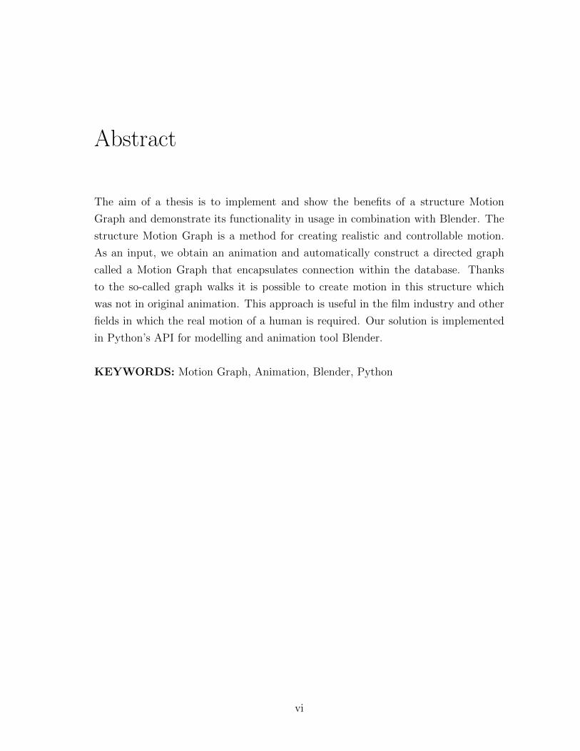
Abstract

The aim of a thesis is to implement and show the benefits of a structure Motion

Graph and demonstrate its functionality in usage in combination with Blender. The

structure Motion Graph is a method for creating realistic and controllable motion.

As an input, we obtain an animation and automatically construct a directed graph

called a Motion Graph that encapsulates connection within the database. Thanks

to the so-called graph walks it is possible to create motion in this structure which

was not in original animation. This approach is useful in the film industry and other

fields in which the real motion of a human is required. Our solution is implemented

in Python’s API for modelling and animation tool Blender.

KEYWORDS: Motion Graph, Animation, Blender, Python

vi

Abstrakt

Ciel’om prace je implementovat’ a ukazat’ vyhody struktury Motion Graph a

demostrovat’ jej funkcionalitu a pouzitie v kombinacii s Blender-om. Struktura Mo-

tion Graph je metoda na vytvaranie realistickeho a kontrolovatel’neho pohybu. Ako

vstup ocakavame animaciu a automaticky skonstruujeme orientovany graf nazyvany

Motion Graph, ktory zahrna prepojenia v databaze poz. V tejto strukture, vd’aka

takzvanym prechadzkam v grafe je mozne vytvorit’ pohyb, ktory nebol v povodnej

animacii. Tento prıstup je uzitocny vo filmovom priemysle a v d’alsıch oblastiach

v ktorych je realnost’ pohybu cloveka potrebna. Nase riesenie je implementovane v

Python API pre modelovacı a animacny nastroj Blender.

KL’UCOVE SLOVA: Struktura Motion Graph, Animacia, Blender, Python

vii

List of Figures

3.1 The skleton A on the left side, skeleton B in the rest pose on other side. 13

3.2 The skleton A and the skeleton B in the same pose. . . . . . . . . . . 14

4.1 The relationship among the animation skeletons, poses and animation

actions in Blender [ble12]. . . . . . . . . . . . . . . . . . . . . . . . . 18

4.2 Control panel in Blender . . . . . . . . . . . . . . . . . . . . . . . . . 30

5.1 Part of the Blender scene using our script. . . . . . . . . . . . . . . . 32

5.2 Extracted key poses from input animation. . . . . . . . . . . . . . . . 34

5.3 Example 1- we set starting and ending pose. . . . . . . . . . . . . . . 35

5.4 Example 1- generated path by graph walk. . . . . . . . . . . . . . . . 35

5.5 Example 2- we set starting and ending pose. . . . . . . . . . . . . . . 36

5.6 Example 2- generated path by graph walk. . . . . . . . . . . . . . . . 36

viii

Contents

Introduction 1

1 Overview of the problem 2

1.1 Basic definitions . . . . . . . . . . . . . . . . . . . . . . . . . . . . . . 2

1.2 Graph Theory . . . . . . . . . . . . . . . . . . . . . . . . . . . . . . 4

1.2.1 Dijstra’s algorithm . . . . . . . . . . . . . . . . . . . . . . . . 5

1.3 Structure Motion Graph . . . . . . . . . . . . . . . . . . . . . . . . . 6

2 Related works and motivation 8

2.1 Motivation . . . . . . . . . . . . . . . . . . . . . . . . . . . . . . . . . 8

2.2 Related works . . . . . . . . . . . . . . . . . . . . . . . . . . . . . . . 9

3 Proposed solution 12

3.1 Description of the subject . . . . . . . . . . . . . . . . . . . . . . . . 12

3.2 Suggested solution . . . . . . . . . . . . . . . . . . . . . . . . . . . . 13

4 Solution 16

4.1 Application possibilities of Blender and Blender Python API . . . . . 16

4.2 Implementation . . . . . . . . . . . . . . . . . . . . . . . . . . . . . . 18

4.2.1 Analysis of the input data . . . . . . . . . . . . . . . . . . . . 19

4.2.2 Creating structure Motion Graph . . . . . . . . . . . . . . . . 20

4.2.3 Structure of the XML file . . . . . . . . . . . . . . . . . . . . 21

4.2.4 ParseXML - Import XML file . . . . . . . . . . . . . . . . . . 22

ix

4.2.5 CreateXML - Export structure to XML file . . . . . . . . . . . 23

4.2.6 Graph walk - Dijkstra’s algorithm . . . . . . . . . . . . . . . . 24

4.2.7 Creating new animation . . . . . . . . . . . . . . . . . . . . . 26

4.2.8 User interface . . . . . . . . . . . . . . . . . . . . . . . . . . . 28

5 Results 31

5.1 Controlling . . . . . . . . . . . . . . . . . . . . . . . . . . . . . . . . 31

5.2 Review of chosen results . . . . . . . . . . . . . . . . . . . . . . . . . 33

Conclusion 37

Bibliography 38

x

Introduction

An animation is a main part of the development in a cinema and entertainment

industry. In the present the virtual persons, so-called virtual agents in the science of

computer animation, occur very often in the film . The virtual agent, human, should

have realistic motion.

One of the possible methods how to add realistic motion to the virtual agent is a

usage of a Motion Capture method. Motion Capture animation uses the real captured

data from real human and allows us to apply these data to the virtual model. One

disadvantage is the price of equipments by which it is possible to capture the motion

of a human. Second disadvantage is the limited possibilities of animation, because of

limitation by human body. Here is the place where our solution can be useful.

Motion Graph structure allows us to create a long varied animation from the small

amount of input data consisting of the set of poses. The variety of the animation

depends upon the specific features of the key poses in the input data.

Our aim is to implement structure which extract necessary data from existing ani-

mation and automatically create own structure. The advantage is that thanks to the

so-called graph walks it is possible to create motion in this structure which was not

in original animation.

In the first chapter we will define some basic terms necessary to understand given

issue. In the next chapter we will mention some related works. The third chapter will

be devoted to a proposed solution, description of a given problem will be summarised.

The details of implementation will be described in the next chapter, also with some

important parts of code. In the last chapter we will present our results.

1

1Overview of the problem

1.1 Basic definitions

For reason of clarity and readability we will explain (define) important terms which

will be used in following thesis.

• Animation - means change of features in computer graphics in time [SK96].

• Articulated structure - structure consisting of finite sequence of fixed seg-

ments(bones), which are each other connected by joints, in which is possible to rotate

with corresponding segments.[WW91]

• Bones - basic building unit of skeleton, parameters of bone is its length and rotation

in relation to the previous bone in the sequence. [WW91]

• Skeleton - tree structure consisting of bones, which are each other connected by

joints. For each bone in the tree, except the root, exists the previous, parental bone.

In the movement itself the parental bone, the angle between it and the following bone

is retained, so by the rotation is in the movement the whole under-tree, in which is

this bone a root. [WW91]

• Mesh - three dimensional polygonal net, which define a shape of the object. Mesh

is defined by the list of its vertices and their coordinates, and also by sequence of

vertices which creates either polygons. There is many other types of representation

but for our work it is not important [ZBSF04].

2

1.1. BASIC DEFINITIONS

• Keyframes - frames, in which animator define key positions and parameters of

object. For all other frames of animation are parameters of object computed by

interpolation or approximation [Par02].

• Skeletal animation - method used for animation of human figure and animals.

Body consist of two parts: polygonal mesh and skeleton. There is a relation between

the model and skeleton, which in the animation deform the surface of the model.

By the movement of bones is possible to define position of the body. Animation is

created by definition the position of bones in the keyframes [Par02].

• XML file - is a simple text-based format for representing structured information:

documents, data, configuration, books, transactions, invoices, and much more. It was

derived from an older standard format called SGML (ISO 8879), in order to be more

suitable for Web use [w3c12].

• Blender - is multiplatform open source 3D software designed for computer model-

ing and animation. Initially was developed by graphic studio NeoGeo and a company

Not a Number Technologies (NaN). From a year 2002 is Blender distributed under

open source licence with support of Blender Foundation. In the presence of writing

this thesis, the last version is 2.6 [ble12].

• Python - is interpreted programming language [pyt12a], which is developed as

open source project. Its formation is dated to the begin of 90’s. Guido van Rossum

was the main engineer. Python is supported over 20 platforms, but at most of its

libraries is available only for Linux, BSD, Mac OS X and Windows. An advantage of

Python is its easy extensibility. Libraries which can be coded in a languace of C or

C++, extend Python in many ways, make available to application interfaces (API)

various programs, in which work like scripting language. This is a case of Blender.

Blender consists of two programming interfaces, Blender Python API and Game-

Engine Python API. In our work we will use Blender Python API, what is a module

collection, which make available a part of internal data and functions of program.

This usage allow us big amount diversified options, for example adding new function

in to a program. With a help of API is possible to create procedural models, scripts

for export and import a many others. Script allow us:

• draw pop up messages, menu, input arrays

3

1.2. GRAPH THEORY

• render graphic user interface (GUI)

• edit objects in a scene

• process various events

• perform changes in 3D view - set visible layers, position of camera..

• import scripts to Blender

• usage of external libraries for Python

1.2 Graph Theory

In mathematics and computer science, graph theory is the study of graphs, mathe-

matical structures used to model pairwise relations between objects from a certain

collection. A graph in this context refers to a collection of vertices or nodes and a

collection of edges or clips that connect pairs of vertices. A graph may be undirected,

meaning that there is no distinction between the two vertices associated with each

edge, or its edges may be directed from one vertex to another. In this section, we

would like to present some definition from Graph Theory [Die06] , because it is close

related to Motion Graph.

• graph - is a pair G = (V,E) of sets satisfying E ⊂ [V ]2, thus, the elements of E

are 2-element subsets of V. The elements of V are the vertices(or nodes, or points) of

the graph G, the elements of E are its edges(or lines).

• adjacent neighbours - Two vertices x,y of G are adjacent, or neighbours, if xy is

an edge of G.

• path - is a non-empty graph P = (V,E) of the form

V = x0, x1, ..., xk

E = x0, x1, x2, ..., xk−1, xk

where the xi are all distinct. The vertices x0 and xk are linked by P and are called

its ends; the vertices x1, ..., xk−1 are the inner vertices of P.

4

1.2. GRAPH THEORY

• length of path - the number of edges of a path is its length.

• cycle - if P = x0, ..., xk−1 is a path and k ≥ 3 then the graph C := P + xk−1x0 is

called cycle.

• connected graph - a non empty graph G is called connected if any two of its

vertices are linked by a path in G.

• component of graph - component of graph G is connected under-graph of graph

G, which is not consists in no bigger connected under-graph of graph G (maximal

connected under-graph).

• cost of path - let G = (V,E) is undirected graph with valued edges, it means for

G is given function h : E→R. Path in graph G is sequence of vertices [v0, v1, ..., vk],

where (vi−1, vi)∈E for i = 1, 2, ..., k. The cost of path P = [v0, v1, ..., vk] isk∑

i=1

h(vi−1,vi).

The cost of path we will mark as |P |.

1.2.1 Dijstra’s algorithm

For a given source vertex in the graph, the algorithm finds the part with lowest cost

or the shortest path between that every other vertex. There is no constrain to use

this algorithm for finding the shortest path between two single vertices by stopping

the algorithm once the shortest path to the destination vertex has been determined.

Djistra’s algorithm runs in worst case in O(|V |2) [Du97]. We will mention here the

pseudocode [wik12]:

function Dijkstra(Graph, source):

for each vertex v in Graph:

dist[v] := infinity ;

previous[v] := undefined ;

end for ;

dist[source] := 0 ;

Q := the set of all nodes in Graph ;

while Q is not empty:

u := vertex in Q with smallest distance in dist[] ;

if dist[u] = infinity:

5

1.3. STRUCTURE MOTION GRAPH

break ;

end if ;

remove u from Q ;

for each neighbor v of u:

alt := dist[u] + dist_between(u, v) ;

if alt < dist[v]:

dist[v] := alt ;

previous[v] := u ;

decrease-key v in Q;

end if ;

end for ;

end while ;

return dist[] ;

end Dijkstra.

1.3 Structure Motion Graph

In this section, we define the motion graph structure [KGP02] and the procedure for

constructing it from a database of clips. A clip of motion is defined as a regular

sampling of the character’s parameters, which consist of the position of the root joint

and quaternions representing the orientations of each joint.

A motion graph is a directed graph where all edges correspond to clips of motion.

Nodes serve as choice points connecting these clips, i.e., each outgoing edge is poten-

tially the successor to any incoming edge. A trivial motion graph can be created by

placing all the initial clips from the database as nodes in the graph. This creates a dis-

connected graph with 2n nodes, one at the beginning and end of each clip(expecting

n clips). Similarly, an initial clip can be broken into two clips by inserting a node,

since the later part of the motion is a valid successor to the earlier part.

A more interesting graph requires greater connectivity. For a node to have multiple

outgoing edges, there must be multiple clips that can follow the clip(s) leading into the

node. Since it is unlikely that two pieces of original data are sufficiently similar, we

need to create edge expressly for this purpose. Transitions are clips designed such that

6

1.3. STRUCTURE MOTION GRAPH

they can seamlessly connect two segments of original data thanks to interpolation.

By introducing nodes within the initial clips and inserting transition clips between

otherwise disconnected nodes, we can create a wellconnected structure with a wide

range of possible graph walks.

Unfortunately, creating transitions is a hard animation problem. Imagine, for exam-

ple, creating a transition between a run and a backflip. In real life this would require

several seconds for an athlete to perform, and the transition motion looks little like

the motions it connects. Therefore the problem of automatically creating such a tran-

sition is complex. On the other hand, if two motions are “close” to each other then

simple blending techniques can reliably generate a transition. How to analyse two

motions and compare them, we will describe in next chapters. In light of this, our

strategy is to identify positions of the initial clips that are sufficiently similar that

straightforward blending is almost certain to produce valid transitions.

How to solve this problem we will describe in the following section.

7

2Related works and motivation

2.1 Motivation

This part is devoted to the necessity of the solution of implementation of the Motion

Graph structure. We will try to show the advantages in comparison with other

animation techniques for creating real human motion. The quoted related papers

dealing with the similar aim is listed below, in the next subchapter.

Motivation of implementing of the Motion Graph structure is to render the most real

human motion. With this approach, we can create a long varied animation from the

small input data consisting of the set of poses. The variety of the animation depends

upon the specific features of the key poses in the input data. This method of Motion

Graph structure is not very expensive because it depends only upon the input model

animation.

Real human motion simulated in the Motion Graph structure is very important from

several points of view. Mostly it is exploited in the film and video-gaming industry. In

both cases, the most real projection of human motion is desired. Despite the fact that

the existing methods in this field are reaching quite a good level of quality, they are

demanding resources which are making the final animation more expensive. Another

disadvantage of these methods is that the final animation is limited by the ability of

the human body movements.

The aim of our thesis is not to improve the existing methods for creating real human

8

2.2. RELATED WORKS

motions, but to reveal the new possible approach by which we do not improve the

quality of final animation from the point of reality of human motion. However the

constraints of the moving apparatus of the human body are removed by our approach

and also the requirements upon the resources are quite low.

2.2 Related works

In this subchapter the paper Motion Graphs of the authors Lucas Kovar, Michael

Gleicher and Frederic Pighin is cited. This paper is very interesting and its part

dealing with the review of the related works is the most representative in this research

field [KGP02].

Much previous work with motion capture has revolved around editing individual clips

of motion. Motion warping [WP95] can be used to smoothly add small changes to a

motion. Retargeting [Gle98],[LS99] maps the motion of a performer to a character of

different proportions while retaining important constraints like footplants. Various

signal processing operations [BW95] can be applied to motion data. My work differs

from the related works in that it involves creating streams of motion, rather than

modifying specific clips.

Another popular approach to motion synthesis is to construct statistical models.

Pullen and Bregler [PB00] used kernel-based probability distributions to synthesize

new motion based on the statistical properties of example motion. Coherence was

added to the model by explicitly accounting for correlations between parameters.

Bowden [Bow00], Galata et al. [GJH01], and Brand and Hertzmann [[BH00]] all

processed motion capture data by constructing abstract “states” which each represent

entire sets of poses. Transition probabilities between states were used to drive motion

synthesis. Since these statistical models synthesize motion based on abstractions of

data rather than actual data, they risk losing important detail. In our work we have

tighter guarantees on the quality of generated motion. Moreover, these systems did

not focus on the satisfaction of high-level constraints.

We generate motion by piecing together example motions from a database. Numer-

ous other researchers have pursued similar strategies. Perlin [Per95] and Perlin and

Goldberg [PG96] used a rulebased system and simple blends to attach procedurally

9

2.2. RELATED WORKS

generated motion into coherent streams. Faloutsos et al. [FvdPT01] used support

vector machines to create motion sequences as compositions of actions generated from

a set of physically based controllers. Since our system involves motion capture data,

rather than procedural or physically based motion, we require different approaches

to identifying and generating transitions. Also, these systems were mainly concerned

with appropriately generating individual transitions, whereas we address the problem

of generating entire motions (with many transitions) that meet user-specified criteria.

Lamouret and van de Panne [LdP96] developed a system that used a database to ex-

tract motion meeting high-level constraints. However, their system was applied to a

simple agent with five degrees of freedom, whereas we generate motion for a far more

sophisticated character. Molina-Tanco and Hilton [MTHMH00] used a state-based

statistical model similar to those mentioned in the previous paragraph to rearrange

segments of original motion data. These segments were attached using linear in-

terpolation. The user could create motion by selecting keyframe poses, which were

connected with a highprobability sequence of states. Our work considers more general

and sophisticated sets of constraints.

Work similar to ours has been done in the gaming industry to meet the requirements of

online motion generation. Many companies use move trees, which (like motion graphs)

are graph structures representing connections in a database of motion. However,

move trees are created manually—short motion clips are collected in carefully scripted

capture sessions and blends are created by hand using interactive tools. Motion graphs

are constructed automatically. Also, move trees are typically geared for rudimentary

motion planning (“I want to turn left, so I should follow this transition”), as opposed

to more complicated objectives. The generation of transitions is an important part

of our approach. Early work in this area was done by Perlin [Per95], who presented

a simple method for smoothly interpolating between two clips to create a blend.

Lee [Lee00] defined orientation filters that allowed these blending operations to be

performed on rotational data in a more principled fashion. Rose et al. [RGBC96]

presented a more complex method for creating transitions that preserved kinematic

constraints and basic dynamic properties.

Our main application of motion graphs is to control a character’s locomotion. This

problem is important enough to have received a great deal of prior attention. Because

a character’s path isn’t generally known in advance, synthesis is required. Procedural

10

2.2. RELATED WORKS

and physically based synthesis methods have been developed for a few activities such

as walking [MD99],[SM01] and running [HWBO95],[BC96]. While techniques such

as these can generate flexible motion paths, the current range of movement styles

is limited. Also, these methods do not produce the quality of motion attainable by

hand animation or motion capture. While Gleicher [Gle01] presented a method for

editing the path traversed in a clip of motion capture, it did not address the need for

continuous streams of motion, nor could it choose which clip is correct to fit a path

(e.g. that a turning motion is better when we have a curved path).

Our basic approach — detecting transitions, constructing a graph, and using graph

search techniques to find sequences satisfying user demands —has been applied previ-

ously to other problems. Schodl et al. [SSSE00] developed a similar method for syn-

thesizing seamless streams of video from example footage and driving these streams

according to high-level user input.

Since writing this thesis, we have learned of similar work done concurrently by a

number of research groups. Arikan and Forsythe [AF02] constructed from a motion

database a hierarchical graph similar to ours and used a randomized search algorithm

to extract motion that meets user constraints. Lee et al. [LCR+02] also constructed a

graph and generated motion via three user interfaces: a list of choices, a sketch-based

interface similar to what we use for path fitting (Section 5), and a live video feed.

Pullen and Bregler [PB02] keyframed a subset of a character’s degrees of freedom and

matched small segments of this keyframed animation with the lower frequency bands

of motion data. This resulted in sequences of short clips forming complete motions.

Li et al [LWyS02] generated a two-level statistical model of motion. At the lower level

were linear dynamic systems representing characteristic movements called “textons”,

and the higher level contained transition probabilities among textons. This model

was used both to generate new motion based on user keyframes and to edit existing

motion.

11

3Proposed solution

3.1 Description of the subject

Before we describe the proposed solution or details of its implementation, we will

recapitulate what kind of problem is solved and which are the aims and requirements

for the final solution. The aim of the work is to study the Motion Graph structure

described in several scientific papers and the implementation of the structure into the

modelling and animating open source tool Blender.

The 3D model animation or the XML file with required input animation data is

supposed as the input data, respectively. The output results in the new animation of

the 3D model with the key poses created from the input, however a different animation

is created. In more details, a required structure is created from the input data and a

new sequence of peaks is created by a graph walk, so the result is a new animation.

The aim of the thesis is as follows:

• to create a tool for the user to create the animations

• to create a realistic animation of articulated model by joining the suitable user

settings and algorithmic constraints

On the other side, to transmission among different 3D models is not the aim of our

thesis.

12

3.2. SUGGESTED SOLUTION

3.2 Suggested solution

Adequate solutions mentioned in the previous chapter are financially and algorithmi-

cally demanding and are almost unavailable to common users. That is why we decided

to implement the Motion Graph structure that can serve as the instrument for cre-

ation of the varied animations for the disposal of the widest range of users. From this

reason we decided to solve the problem in the form of script for the modelling and

animating open source tool Blender, created in programming language Python.

Basic principle

The basic principle of the whole script will be the transmission of the pose of skeleton

A to the identical skeleton B, see the figure 3.1. The way how to reach this trans-

mission is to iterate the skeleton A by the individual bones and to assign the matrix

of each bone in skeleton A to the bone in skeleton B in the same function from the

hierarchy point of view. The basic aim after the pose transmission is to set the pose of

skeleton B to the pose of skeleton A, as we can see in figure 3.2. We want to preserve

only the pose, not the position in the scene coordinates.

Figure 3.1: The skleton A on the left side, skeleton B in the rest pose on other side.

13

3.2. SUGGESTED SOLUTION

Figure 3.2: The skleton A and the skeleton B in the same pose.

Analysis of the input animation data

The analysis of the input animation data will be realised prior the structure creation

itself, in order to extract the key poses of articulated model, which will be the basis in

the creation of peaks in graph. Simultaneously with this analysis we will gain further

important data on the animation scene as, for example, part of the active animation

for the algorithm optimization.

Creation of Motion Graph structure

Owing to complete animation analysis we are able to create a graph represented by

the incident matrix. We will consider the non-oriented graph with valued edges.

Their value will determined by the difference of the key poses in the input data. The

difference between poses will help us to create graph walks. We will keep in other

list the pose of skeleton in certain key frame, which will be nothing else as the set of

matrices. Every matrix will be assigned to the suitable bone.

Exporting of the structure Motion Graph into XML file

For application and usability of this solution we will implement the possibility of

exporting the animation or structure into the XML file. This file will consist of the

most important data for the repeated animation and structure creation. The XML

14

3.2. SUGGESTED SOLUTION

file structure will be described in the following text.

Importing XML file

In this step we will import the initial animation. Parsing the input data is the step

before creating structure. We expect XML file in a format which will be described in

the next chapter.

Graph walk

After creation of Motion Graph structure, user will set constraints and starting and

ending node. We will search for a best fit path between those two nodes. Implemen-

tation of search algorithm we will describe in next chapter. Algorithm output will be

sequence of nodes.

Creation of the output animation

Animation will be created by the graph walk on the basis of the parameters deter-

mined by the user and determined sequence of vertices by graph walk algorithm. It

is very important to choose a suitable sequence of peaks to gain the most faithful

animation.

15

4Solution

4.1 Application possibilities of Blender and Blender

Python API

As our solution is implemented in the form of a script and is the part of the modelling

and animating open source tool Blender and is created in the applied programme

interface Blender Python API, it is reasonable to mention in this chapter which

possibilities for the implementation the programme Blender provide us with. We will

briefly describe the way how the mentioned elements work and what is the relationship

among them like.

Armatures

The skeleton (called armature in Blender) consists of the bones, which are in the rest

position. There is an access to the rest position of the skeleton in the Edit Mode of

the Blender scene. The bones of armature in the rest position will be called as data

bones.

The bones therefore form a hierarchy. The full transform of a child node is the

product of its parent transform and its own transform. So moving a thigh bone

will move the lower leg too. As the character is animated, the bones change their

transformation over time, under the influence of some animation controller. A rig is

generally composed of both forward kinematics and inverse kinematics parts that may

interact with each other. Skeletal animation is referring to the forward kinematics

16

4.1. APPLICATION POSSIBILITIES OF BLENDER AND BLENDER PYTHON API

part of the rig, where a complete set of bones configurations identifies a unique pose.

Pose

The pose defines changes and relationships in the skeleton in the object level. A

corresponding pose channel is created for each bone in the skeleton. In the pose

channel the translations, rotations and scaling of the bone are recorded with respect

to the basic rest position of the skeleton. The pose of the skeleton is accessible via

the Pose Mode of the skeleton in the scene. Its bones will be called the pose bones.

Action

The Action stores the Animation Curves (Ipos) for the PoseChannels and its Con-

straints. You can define an Action as the ”Ipo bag”, the collection of all animated

changes you want to be applied to Poses.

Whether an ”Action Channel” works on a specific Pose Channel is defined by the

Action Channel name. Therefore an Action doesn’t have to be directly derived from

an Armature, it can have fewer channels and can potentially work on different Poses

as well.

Typical Actions can be walkcycles, jumps, waving, grasping, and so on... and be

combined (stacked/strung together) within the NLA editor. The NLA editor actually

creates a ’working Pose’, applies Actions to it, and blends that Pose with the actual

Pose.

There is a possibility to choose one of three basic rotational representations for the

rotations of every object, including skeletons and bones in them:

• Quaternions(’QUATERNION’)

• Euler angles(’XYZ’,’XZY’,’YXZ’,’YZX’,’ZXY’,’ZYX’)

• Rotation with the help of axis and angle(axis-angle representation(AXIS AN-

GLE))

17

4.2. IMPLEMENTATION

Figure 4.1: The relationship among the animation skeletons, poses and animationactions in Blender [ble12].

4.2 Implementation

The details of the implementation of the solution is described in this chapter. The

methods we used and all relevant parts of their codes are mentioned. Several problems

arising with the implementation and the decisions we have made to overcome these

complications are discussed.

A scene with a mesh object to which an animation skeleton is bounded is the input for

the script. The skeleton of the source object has assigned its own animation action

with the data of the movement determined for the creation of the Motion Graph

structure. To mark the object at first is necessary for the obvious assignment of the

source of input data. It is supposed that the animation action will be created by the

18

4.2. IMPLEMENTATION

user itself or he will have a certain action already at the dispose.

4.2.1 Analysis of the input data

The first analysis of the movement source will take place prior the whatever change in

the input model with assigned animation action. In the analysis all the key frames of

the source animation action will be extracted and for the further run of the programme

the following data will be saved:

• list of bones which contains the articulated model with their locations

• list of key frames

• detect active time line of 3D model in the current scene

def analyze_animation(source):

#set of bone name

bones_names = []

for bone in source.pose.bones:

bones_names.append(bone.name)

print(bones_names)

#set of bone location

bones_location = []

for bone in source.pose.bones:

bones_location.insert(bones_names.index(bone.name),bone.location)

print(bones_location)

#animation frame range

scn = bpy.context.scene

frame_range = source.animation_data.action.frame_range

print(frame_range)

begin = frame_range[0]

end = frame_range[1]

19

4.2. IMPLEMENTATION

# find key frames

scn.frame_set(begin - 1)

global key_frames

key_frames = []

key = -1

before = -2

while key != before:

before = key

bpy.ops.screen.keyframe_jump()

key = scn.frame_current

if key != before:

key_frames.append(key)

print(key_frames)

bpy.ops.object.mode_set(mode=’OBJECT’)

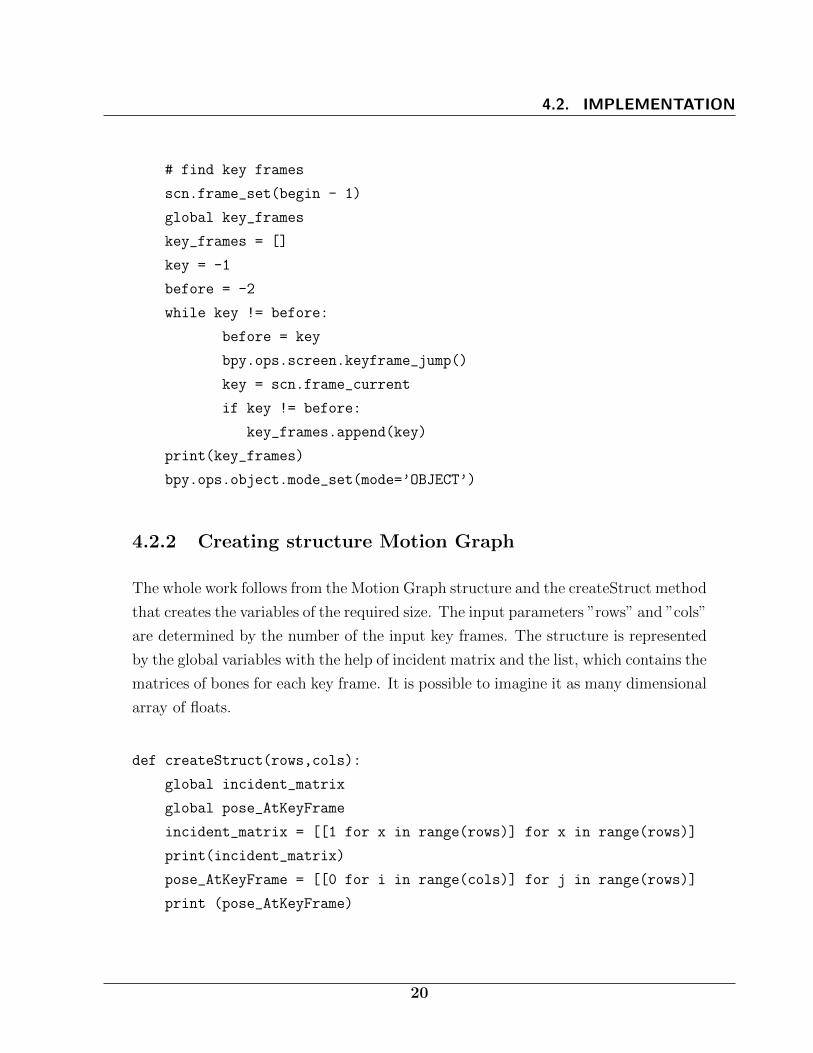
4.2.2 Creating structure Motion Graph

The whole work follows from the Motion Graph structure and the createStruct method

that creates the variables of the required size. The input parameters ”rows” and ”cols”

are determined by the number of the input key frames. The structure is represented

by the global variables with the help of incident matrix and the list, which contains the

matrices of bones for each key frame. It is possible to imagine it as many dimensional

array of floats.

def createStruct(rows,cols):

global incident_matrix

global pose_AtKeyFrame

incident_matrix = [[1 for x in range(rows)] for x in range(rows)]

print(incident_matrix)

pose_AtKeyFrame = [[0 for i in range(cols)] for j in range(rows)]

print (pose_AtKeyFrame)

20

4.2. IMPLEMENTATION

This method is called during the parsing of the input XML file. The structure of

required size will be created by the help of createStruct method. In the next step of

parsing the structure will be filled in by input data in XML file.

4.2.3 Structure of the XML file

In this we will describe proposed structure of the XML file. As the root tag is ”frames”

set. This tag has to properties, armature’s count of bones and number of key frames.

An example you can see below:

<?xml version="1.0"?>

<!--3D model bones-->

<frames count_bones="2" count="3">

<frame id_keyframe="0">

<frame id_keyframe="1">

<frame id_keyframe="2">

</frames>

This root tag is consisted from a tag named ”frame”. It has only one property, it is

used for identification of given key frame. In this tag we store data of armature in

some pose, it mean matrix for every bones of armature. Example of the structure:

<frame id_keyframe="0">

<bone id_keyframe="0" id_bone="0">

<bone id_keyframe="0" id_bone="1">

</frame>

The last we had to define is named ”bone”. It has two properties, identifier of the

key frames and identifier of the bone in armature to which is assigned a matrix stored

in this tag. See example:

<bone id_keyframe="0" id_bone="1">

0,0,0,0,0,0,0,0,0

</bone>

21

4.2. IMPLEMENTATION

4.2.4 ParseXML - Import XML file

In this part we will describe method which creates structure Motion Graph from XML

file. For parsing we use XML dom.minidom library [pyt12b]. It helps as to divide the

file in to tags, then by iterating to extract further data and rebuild Motion Graph

structure.

def parseXML(file_path):

global pose_AtKeyFrame

#open the xml file for reading:

file = open( file_path,’r’)

#convert to string:

data = file.read()

#close file because we dont need it anymore:

file.close()

#parse the xml you got from the file

dom = parseString(data)

element_node_list = dom.getElementsByTagName("frames")

element_n = element_node_list[0]

count_keyframes = int(element_n.attributes["count"].value)

count_bones = int(element_n.attributes["count_bones"].value)

createStruct(count_keyframes,count_bones)

element_node_list = dom.getElementsByTagName("bone")

for i in range(0,element_node_list.length):

element_n = element_node_list[i]

id_keyframe = int(element_n.attributes["id_keyframe"].value)

id_bone = int(element_n.attributes["id_bone"].value)

data = element_n.firstChild.data

kf = []

array = data.rsplit(’,’)

for x in array:

x = float(x)

kf.append(x)

newMat = Matrix(((kf[0], kf[1], kf[2], kf[3]),

22

4.2. IMPLEMENTATION

(kf[4],kf[5],kf[6], kf[7]),

(kf[8], kf[9], kf[10], kf[11]) ,

(kf[12], kf[13], kf[14], kf[15])))

pose_AtKeyFrame[id_keyframe][id_bone] = newMat

print("#---BONE---#")

print (id_keyframe)

print (id_bone)

print (newMat)

4.2.5 CreateXML - Export structure to XML file

This method provide us opportunity to create some animation using Motion Graph

structure and export it to XML file for next work. We fill in the structure of XML

file from the structure, in case of only exporting animation, on the back we create a

structure for easier implementation.

def createXML(path):

global key_frames

global pose_AtKeyFrame

doc = minidom.Document()

doc.appendChild(doc.createComment("3D model bones"))

frames = doc.createElement(’frames’)

frames.setAttribute("count",str(len(key_frames)))

frames.setAttribute("count_bones",str(len(bpy.data.objects[0].pose.bones)))

doc.appendChild(frames)

for j in range(0,len(key_frames)):

name = "frame"

fr = doc.createElement(name)

fr.setAttribute("id_keyframe", str(j))

frames.appendChild(fr)

for i in range(0,len(pose_AtKeyFrame[j])):

23

4.2. IMPLEMENTATION

name = "bone"

obj = doc.createElement(name)

obj.setAttribute("id_bone", str(i))

obj.setAttribute("id_keyframe", str(j))

data = matrixToString(pose_AtKeyFrame[j][i])

obj.appendChild(doc.createTextNode(data))

fr.appendChild(obj)

print (doc.toprettyxml(indent = ’ ’))

file = open(path, ’w’)

file.write(doc.toxml())

4.2.6 Graph walk - Dijkstra’s algorithm

After the creation of structure, we are getting to the core of our thesis. As we have

mentioned before, the graph structure is represented by incident matrix. The next

step is the evaluation of the edges between the individual peaks. In this step we had to

make a decision, how to implement the evaluation function of the edges. The approach

we have chosen is straight-lined. The values of edges are in direct dependence upon

distinctions of two vertices, it means, difference between the poses stored in each

vertex. For example, if two poses are quite similar, the value of the edge is near zero

and on the other hand in case of two various poses the edge value is increasing up

to number of bones in armature. This is very useful, because we want to find such

a path in graph between two vertices, in which there are not great differences(edge

values) between individual adjacent vertices. That is the same problem like to find

the lowest cost path between two peaks.

Two poses are compared in such a way, that we take bone matrix from one pose, a

bone matrix from another pose and we make a difference between every two adequate

elements of matrices. If the difference is smaller than a chosen threshold, we continue

in computing. Otherwise we return the response, that the given matrices are not

similar enough. The edge value consists of value of a count of various matrices between

two poses of the adequate bones.

24

4.2. IMPLEMENTATION

def compare_pose(pose1_id, pose2_id, treshold):

global bones_names

global pose_AtKeyFrame

value = 0

pose1 = pose_AtKeyFrame[pose1_id]

pose2 = pose_AtKeyFrame[pose2_id]

for i in range(0,len(pose1)):

matrix1 = pose1[i].to_3x3()

matrix2 = pose2[i].to_3x3()

if not compare_matrices(matrix1, matrix2, treshold):

value = value + 1

return value

After the edge assessment we can continue with graph walk. The user is asked to

determine the starting and the end peak and the required threshold value. It enables

to remove the edge that joins two different poses so the edge is of a greater value than

the threshold.

With this setting a guaranty will be achieved, that transitions among the

poses(vertices) will be chosen with lower difference. This sequence of steps will lead

to the smoother animation. For the reason of better implementation we create the

representation by the field of neighbours from the adjacent matrix. In this new field

there are added edges with lower value than the threshold value. After the graph

walk this structure is deleted. Thanks to this copy, we do not have to calculate the

deleted edge, which do not fulfil the threshold rule.

At first, we verify if two chosen vertices are in the same component and so it has

a sense to compute the lowest cost path between them. For this purpose we use

depth-first search. If they are not located in one component, a warning is given to

the Toggle Console. In another case, an algorithm for searching of the lowest cost

path between these two vertices will be run. For solving of this problem the Dijstra’s

algorithm is used. It is described in detail in chapter 1. Our implementation follows,

as we do not need to compute the distances from the starting node to all in the graph,

but only to single given node.

def djistra(graph,start,end,visited=[],distances={},predecessors={}):

25

4.2. IMPLEMENTATION

global bignum

if start==end:

path=[]

while end != None:

path.append(end)

end=predecessors.get(end,None)

return distances[start], path[::-1]

if not visited: distances[start]=0

for neighbor in graph[start]:

if neighbor not in visited:

neighbordist = distances.get(neighbor,bignum)

tentativedist = distances[start] + graph[start][neighbor]

if tentativedist < neighbordist:

distances[neighbor] = tentativedist

predecessors[neighbor]=start

visited.append(start)

unvisiteds = dict((k, distances.get(k,bignum))

for k in graph if k not in visited)

closestnode = min(unvisiteds, key=unvisiteds.get)

return djistra(graph,closestnode,end,visited,distances,predecessors)

After the gaining of the lowest cost path the sequence of nodes will be stored for

further usage in creation of resulting animation described in the following text.

4.2.7 Creating new animation

In this part we describe creating of output, a new animation. As a input parameter we

gain a sequence of nodes, computed by Djistra’s algorithm. On the user instruction

we start computing.

Several important methods which we use in the animation creation are described in

the following text.

def animate(target, key_frames):

26

4.2. IMPLEMENTATION

global pose_frame

global next_frame

global frame_dist

global start_frame

bpy.ops.object.mode_set(mode=’POSE’)

for bone in target.bones:

bone.select = True

scn = bpy.context.scene

scn.frame_start = 1

scn.frame_end = 100

before = 0

for f in key_frames:

print(pose_frame)

scn.frame_set(start_frame+next_frame)

ret_source(target,f)

bpy.ops.anim.keyframe_insert_menu(type=’LocRot’)

next_frame = next_frame + frame_dist

bpy.ops.screen.animation_play()

This method gets parameters as target armature and set of the key frames. In software

Blender it is very important in which mode the scene is set. From this mode set

depends the set of possibilities that we can execute. The choosing of the Pose Mode

is also important because in this mode we can work with the skeleton pose, it means

to change the position of simple bones. The further logic step is the need to mark

each bone of the skeleton in order to determine what we would like to work with in the

scene. The cycle in which we will iterate each key frame from the input set consisting

of key frames will follow. The pose of skeleton in each key frame will be applied at

first on the selected set of bones and then the new key frame will be inserted in the

scene. After this operation the created animation will be run in preview, it means,

the frames between two key frames will be by linear interpolation software Blender

computed.

The next function will be described that directly applies the data from the poses of

each bone from a certain peak in the graph to the skeleton in the scene. This function

27

4.2. IMPLEMENTATION

is the base of the script.

def ret_source(target,frame):

bpy.ops.object.mode_set(mode=’POSE’)

size = 0

for bone in target.pose.bones:

bone.matrix = pose_AtKeyFrame[frame][size]

size +=1

In this function the matrices of each bone are directly assigned to its image in target

skeleton. This process will guarantee that the skeleton in the scene will gain the pose

that is saved in the given peak. It means, that key pose from the input animation,

stored in the certain peak in graph, is applied to given skeleton in the scene.

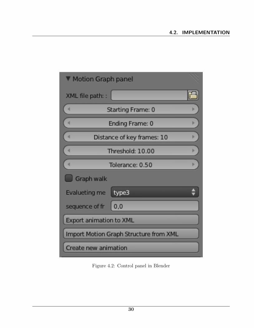
4.2.8 User interface

In order to control simply the creation of the animations with the help of the Motion

Graph structure we have added a special panel implemented in Blender GUI. The

user can choose by marking the target object, the path to XML file for loading of the

structure in case of need and a lot of further settings. After setting of the required

parameters in dependence upon the situation the user has a possibility to push the

buttons according to the given situation and to export the structure to XML file,

to import the structure from XML file or to run the creation of a new animation in

dependence of the given parameters and sequence of key frames.

The example how the defined button and its method execute will be performed after

the pushing of the button is as follows:

class OBJECT_OT_Input_Button(bpy.types.Operator):

bl_idname = "input.animation"

bl_label = "Export animation to XML"

def execute(self, context):

global key_frames

28

4.2. IMPLEMENTATION

scn = context.scene

bpy.ops.wm.console_toggle()

bpy.ops.object.mode_set(mode=’OBJECT’)

# choose selected object in the scene

name_of_selected_object = bpy.context.active_object.name

armature = bpy.data.objects[name_of_selected_object]

analyze_animation(armature)

createStructure(armature)

createXML()

return{’FINISHED’}

29

4.2. IMPLEMENTATION

Figure 4.2: Control panel in Blender

30

5Results

These chapter is dedicated to the results of our solving of the implementation structure

Motion Graph into the modelling and animating tool Blender. We will describe the

usage and controlling of the script and also we will present the samples of generated

animations from the structure.

5.1 Controlling

As first, is needed to do some changes on 3D model settings. The thing we have to

change is the settings of bones. Change your mode to edit mode. For each bone,

select it, in right panel in Blender, choose the bookmark ”Bone” and deselect the box

Inherit Rotation and select Connected(in case this bone should be connected to the

parent bone).

After the script is installed or run a possibility to work with the structure Motion

graph is gained from the text editor integrated in the Blender.

In this moment there is a possibility to choose (select) one from three actions:

1 – a structure from the XML file can be imported

2 – an animation into XML file can be exported

3 – a new animation with the help of the structure Motion Graph can be created.

31

5.1. CONTROLLING

When using it the blender console is required to be open. This can be found in the

item Help –Toggle Console. In this window the relevant (potential) warnings occur

during the work with our script.

When the Motion Graph structure is already created, there are two possible ways how

to create a new animation. The first way is to mark a Boolean Graph walk. With this

option (set-up, setting, positioning) it is obligatory to set the Starting Key Frame and

Ending Key Frame. A number of the Key Frame is its index and the numbering starts

from 0. In the lower part of the scene there is a timeline, where the user can easily

find out (recognize, determine) from which key frame he would like to start the walk

and in which key frame to finish it. With this selection the setting of the Threshold

value is very important. This value will remove (eliminate) the edges with higher

value in comparison with the given value. After stroking Create new animation a

lowest cost path between two given vertices will be found in the graph by our script.

In case the Graph walk is not stroked (marked), the user has a possibility to simply

insert id of the individual (separate) key frames into the field sequence of frames. In

this case the lowest cost path will not be found, but the interpolation between the

given peaks is used. For each of these two possibilities it is possible to choose an

additional setting of a key frame distance in the resulting animation.

Figure 5.1: Part of the Blender scene using our script.

32

5.2. REVIEW OF CHOSEN RESULTS

5.2 Review of chosen results

When testing our solution a 3D model of humanoid armature was used. Naturally

our solution is implemented in such a way, that it could be for any 3D model with a

bound armature. In the figure 5.2 the poses extracted from the initial animation are

presented. They are numbered in order to make it more transparent. The results of

our graph walk algorithm between two peaks selected by the user are demonstrated.

In some cases the animation is the same in both cases (examples, situations) because

the selected two poses were similar and so the lowest cost path was directed via the

edges between them. For these two approaches(graph walk and basic interpolation)

we tried to select the examples with two non-identical animations. Perhaps the results

would be more attractive if the armature animation with a really great number of the

key frames had been at the disposal. However, our animation is satisfying (suitable,

convenient) to demonstrate the functionality of the solution, too.

33

5.2. REVIEW OF CHOSEN RESULTS

Figure 5.2: Extracted key poses from input animation.

34

5.2. REVIEW OF CHOSEN RESULTS

Figure 5.3: Example 1- we set starting and ending pose.

Figure 5.4: Example 1- generated path by graph walk.

35

5.2. REVIEW OF CHOSEN RESULTS

Figure 5.5: Example 2- we set starting and ending pose.

Figure 5.6: Example 2- generated path by graph walk.

36

Conclusion

In our thesis we were dealing with the implementation of the structure motion graph

that serves as a tool for generating the new original animations. To study a given

structure and to implement it later into the modeling and animating tool Blender

was the main aim of this thesis.

In Chapter 1 several basic terms were introduced, the knowledge of which is necessary

to understand this thesis. First of all we tried to understand the graph theory. In

Chapter 2 we were discussing the motivation of this work and why is it so interesting

to solve a given issue. The already published related works have been mentioned, too.

In the next chapter the issue that is discussed was resumed and a suggested solution

was described. In Chapter 4 a precise implementation of solution was described,

especially the usage of the algorithm on the graph structure.

Solution in the form of a script in the modelling and animating tool Blender was

implemented. It is assumed that a wide range of the users could exploit (use) it.

Now it is suitable to summarize the results of our thesis and its possible benefits. With

our solution the implementation of the extracted key frames from the animation was

successful. The next step was the creation of the motion graph structure. A decision

followed on how to compare the individual key poses and the evaluation function

was implemented. Finally the algorithm proposal for finding the most suitable path

between two chosen vertices was realized.

These results are satisfying, but it will be very interesting to deal with the following

issues in the future. It would be suitable to deal with the task how to compare two

poses in a more effective way, how to decide whether two poses are similar enough,

i. e. to create a satisfactory animation by the interpolation of their data. Second

interesting task for improving results is the optimalization of the graph walk algorithm

to get smoother animations .

37

Bibliography

[AF02] Okan Arikan and D. A. Forsyth. Interactive motion generation from

examples. ACM Trans. Graph., 21(3):483–490, July 2002.

[BC96] Armin Bruderlin and Tom Calvert. Knowledge-driven, interactive ani-

mation of human running. In IN GRAPHICS INTERFACE ’96, pages

213–221, 1996.

[BH00] Matthew Brand and Aaron Hertzmann. Style machines. In Proceedings

of the 27th annual conference on Computer graphics and interactive

techniques, SIGGRAPH ’00, pages 183–192, New York, NY, USA, 2000.

ACM Press/Addison-Wesley Publishing Co.

[ble12] Blender foundation, May 2012. http://www.blender.org/.

[Bow00] Richard Bowden. Learning statistical models of human motion, 2000.

[BW95] Armin Bruderlin and Lance Williams. Motion signal processing. In

Proceedings of the 22nd annual conference on Computer graphics and

interactive techniques, SIGGRAPH ’95, pages 97–104, New York, NY,

USA, 1995. ACM.

[Die06] R. Diestel. Graph Theory. Graduate Texts in Mathematics. Springer,

2006.

[Fra11] Roman Franta. Motion retargeting between articulated structures. Fac-

ulty of Mathematics, Physics and Informatics, Comenius University,

2011.

[FvdPT01] Petros Faloutsos, Michiel van de Panne, and Demetri Terzopoulos.

Composable controllers for physics-based character animation. In Pro-

ceedings of the 28th annual conference on Computer graphics and in-

teractive techniques, SIGGRAPH ’01, pages 251–260, New York, NY,

USA, 2001. ACM.

[GJH01] Aphrodite Galata, Neil Johnson, and David Hogg. Learning variable

length markov models of behaviour. Computer Vision and Image Un-

derstanding, 81:398–413, 2001.

38

BIBLIOGRAPHY

[Gle98] Michael Gleicher. Retargetting motion to new characters. In Proceed-

ings of the 25th annual conference on Computer graphics and interactive

techniques, SIGGRAPH ’98, pages 33–42, New York, NY, USA, 1998.

ACM.

[Gle01] Michael Gleicher. Motion path editing. In Symposium on Interactive

3D Graphics, pages 195–202, 2001.

[HWBO95] Jessica K. Hodgins, Wayne L. Wooten, David C. Brogan, and James F.

O’Brien. Animating human athletics. In Proceedings of the 22nd an-

nual conference on Computer graphics and interactive techniques, SIG-

GRAPH ’95, pages 71–78, New York, NY, USA, 1995. ACM.

[KGP02] Lucas Kovar, Michael Gleicher, and Frederic Pighin. Motion graphs. In

Proceedings of the 29th annual conference on Computer graphics and

interactive techniques, SIGGRAPH ’02, pages 473–482, New York, NY,

USA, 2002. ACM.

[LCF05] Yu-Chi Lai, Stephen Chenney, and ShaoHua Fan. Group motion

graphs. In Proceedings of the 2005 ACM SIGGRAPH/Eurographics

symposium on Computer animation, SCA ’05, pages 281–290, New

York, NY, USA, 2005. ACM.

[LCR+02] Jehee Lee, Jinxiang Chai, Paul S A Reitsma, Jessica K Hodgins, and

Nancy S Pollard. Interactive control of avatars animated with human

motion data. Proceedings of the 29th annual conference on Computer

graphics and interactive techniques SIGGRAPH 02, 21(3):491, 2002.

[LdP96] A. Lamouret and M. Van de Panne. Motion synthesis by example. In

EGCAS ’96: Seventh International Workshop on Computer Animation

and Simulation, 1996.

[Lee00] Jehee Lee. A hierarchical approach to motion analysis and synthesis

for articulated figures, 2000.

[LS99] Jehee Lee and Sung Yong Shin. A hierarchical approach to inter-

active motion editing for human-like figures. In Proceedings of the

39

BIBLIOGRAPHY

26th annual conference on Computer graphics and interactive tech-

niques, SIGGRAPH ’99, pages 39–48, New York, NY, USA, 1999. ACM

Press/Addison-Wesley Publishing Co.

[LWyS02] Yan Li, Yan L Tianshu Wang, and Heung yeung Shum. Motion texture:

A two-level statistical model for character motion synthesis. In ACM

Transactions on Graphics, pages 465–472, 2002.

[MD99] Franck Multon and Gilles Debunne. Computer animation of human

walking: a survey, 1999.

[MTHMH00] Luis Molina-Tanco, Adrian Hilton, Luis Molina, and Tanco Adrian

Hilton. Realistic synthesis of novel human movements from a database

of motion capture examples. In In Workshop on Human Motion

(HUMO’00, pages 137–142, 2000.

[Par02] R. Parent. Computer Animation: Algorithms and Techniques. Mor-

gan Kaufmann Series in Computer Graphics and Geometric Modeling.

Morgan Kaufmann, 2002.

[PB00] Katherine Pullen and Christoph Bregler. Animating by multi-level sam-

pling. In Proceedings of the Computer Animation, CA ’00, pages 36–,

Washington, DC, USA, 2000. IEEE Computer Society.

[PB02] Katherine Pullen and Christoph Bregler. Motion capture assisted ani-

mation: Texturing and synthesis, 2002.

[Per95] Ken Perlin. Real time responsive animation with personality. IEEE

Transactions on Visualization and Computer Graphics, 1(1):5–15,

March 1995.

[PG96] Ken Perlin and Athomas Goldberg. Improv: A system for scripting

interactive actors in virtual worlds, 1996.

[pyt12a] Python, May 2012. http://www.python.org/.

[pyt12b] Python documentation, May 2012. http://www.docs.python.org/.

[RF95] Eugen Ruzicky and Andrej Ferko. Pocıtacova grafika a spracovanie

obrazu. Sapientia, 1995.

40

BIBLIOGRAPHY

[RGBC96] Charles Rose, Brian Guenter, Bobby Bodenheimer, and Michael F. Co-

hen. Efficient generation of motion transitions using spacetime con-

straints. In Proceedings of the 23rd annual conference on Computer

graphics and interactive techniques, SIGGRAPH ’96, pages 147–154,

New York, NY, USA, 1996. ACM.

[SK96] Laszlo Szirmay-Kalos. Theory of Three Dimensional Computer Graph-

ics. Akademiai Kiado, Budapest, 1996.

[SM01] Harold C. Sun and Dimitris N. Metaxas. Automating gait generation.

In SIGGRAPH, pages 261–270, 2001.

[SSSE00] Arno Schodl, Richard Szeliski, David H. Salesin, and Irfan Essa. Video

textures. In Proceedings of the 27th annual conference on Computer

graphics and interactive techniques, SIGGRAPH ’00, pages 489–498,

New York, NY, USA, 2000. ACM Press/Addison-Wesley Publishing

Co.

[Du97] Pavol Duris. Tvorba efektıvnych algoritmov. Katedra informatiky FMFI

UK, 1997.

[w3c12] World wide web consortium, May 2012. http://www.w3.org/.

[wik12] Wikipedia, diijstra, May 2012. http://wwwhttp://en.wikipedia.

org/wiki/Dijkstra’s_algorithm/.

[Woo04] Oliver Edward Wood. Autonomous Characters in Virtual Environ-

ments: The technologies involved in artificial life and their affects of

perceived intelligence and playability of computer games. PhD thesis,

2004.

[WP95] Andrew Witkin and Zoran Popovic. Motion warping. In Proceedings

of the 22nd annual conference on Computer graphics and interactive

techniques, SIGGRAPH ’95, pages 105–108, New York, NY, USA, 1995.

ACM.

[WW91] Alan Watt and Mark Watt. Advanced animation and rendering tech-

niques. ACM, New York, NY, USA, 1991.

41

[XTK] Jianfeng Xu, Koichi Takagi, and Ryoichi Kawada. Automatic Compo-

sition of Motion Capture Animation for Music Synchronization. pages

85–88.

[ZBSF04] Jirı Zara, Bedrich Benes, Jirı Sochor, and Petr Felkel. Modernı

pocıtacova grafika. Computer Press, 2004.