Motion Equations Proper for Forward Dynamics of Robotic Manipulator … · 2017-11-28 · algorithm...

Transaction B: Mechanical EngineeringVol. 16, No. 6, pp. 479{495c Sharif University of Technology, December 2009

Motion Equations Proper for Forward Dynamicsof Robotic Manipulator with Flexible Links by

Using Recursive Gibbs-Appell Formulation

M.H. Korayem1;� and A.M. Shafei1

Abstract. In this article, a new systematic method for deriving the dynamic equations of motionfor exible robotic manipulators is developed by using the Gibbs-Appell assumed modes method. Theproposed method can be applied to the dynamic simulation and control system design of exible roboticmanipulators. In the proposed method, the link de ection is described by a truncated modal expansion.All the mathematical operations are done by only 3� 3 and 3� 1 matrices. Also, all dynamic expressionsof a link are expressed in the same link local coordinate system. Based on the developed formulation, analgorithm is proposed that recursively and systematically derives the equation of motion, then this methodis compared with the recursive Lagrangian method. As shown, this method is computationally simplerand more e�cient and it reduces a large amount of computational complexity. Finally, a computationalsimulation for a manipulator with two elastic links is presented to verify the proposed method.

Keywords: Manipulator; Flexible link; Recursive; Gibbs-Appell; Complexity.

INTRODUCTION

The derivation of dynamic equations of motion describ-ing the dynamic behavior of robotic manipulators isnecessary for dynamic simulation and control systemdesign. Today, many systematic methods can be usedfor deriving the dynamic equations of robotic manip-ulators [1-3]. But, these methods are only suitablewhen the individual links of a robotic manipulator areassumed rigid.

Based on recent advances in robot utilizationand also the demand for faster robots with greatquality, a light robot usage idea is represented. Robotswith elastic links are introduced as a solution for thedeformation phenomena in light robots with heavyloads. In this case, deformation causes accuracyreduction and system instability. Therefore, there is anobvious requirement for a complete dynamical modelfor this kind of robot to control light links at highvelocity and in heavy load situations, appropriately.The two main approaches for the dynamic modeling

1. Department of Mechanical Engineering, Iran University ofScience and Technology, Tehran, P.O. Box 13114-16846,Iran.

*. Corresponding author. E-mail: [email protected]

Received 9 September 2008; received in revised form 14 January2009; accepted 14 April 2009

of exible robotic manipulators are the �nite elementmethod [4] and the assumed modes method [5-9]. The�nite element method is a general method and can beapplied to manipulators with complex shaped links.But, this method requires sophisticated software forperforming assembly and the order reduction of theelement equations.

The assumed mode method of modeling exiblemanipulators is mainly presented by Book [5]. Herepresented the link deformation and kinematics of rev-olute joints with a 4�4 matrix and used modal analysisfor link deformations. This method of formulation hadacceptable e�ciency in comparison with other methodsof that time. King applied Walker-Orin's method,based on Newton-Euler formulation, to improve Book'smethod [6]. But, his method still su�ered from greatcomputational complexity. Jin and Sankar also have asystematic approach for elastic links [7]. They obtaineddynamical equations by using Lagrange formulationand the modes approach assumption. In this method3 � 3 matrixes are used for computations and theresults are simulated for a robot with one link. Thecomputations, however, are massive.

Highly e�cient multi- exible-body methods havebeen previously presented by Anderson [10] and Baner-jee [11] based on Kane's Method with many other com-parably e�cient multi- exible-body routines developed

480 M.H. Korayem and A.M. Shafei

by E. Haug, J. Angeles, R. Singh, R. Schwertassek,A. Jain, R. Wehage, J. Ambrosio and others [12].Many of these methods are so-called O(N) routines,being able to form equations of motion with an overallcost that increases only linearly with the number ofsystem degrees of freedom N , (for rigid body systems).For exible body systems, this overall cost (equationsformation) is adjusted somewhat, being approximatedas O(n2

f �m2).Dynamic equations of motion by the Gibbs-

Appell formulation begin with a de�nition of Gibbs'function (acceleration energy) [13]. Then, a set ofindependent quasi velocities (linear combination ofgeneralized velocities) should be selected. By takingthe derivative of the Gibbs' function, with respect toquasi accelerations (time derivate of quasi velocities),and equalizing them with generalized forces, theseequations will be obtained. But, this method has beenthe least used for resolution of the dynamic problemof manipulating robots. In the �eld of robotics,Popov proposed a method later developed by Vuko-bratovic and Potkonjak in which the G-A equationswere used to develop a closed form representation ofhigh computational complexity [14]. This method wasused by Desoyer and Lugner to solve, by means ofa recursive formulation, O(n2), the inverse dynamicproblem, using the Jacobian matrix of the manipulatorwith the purpose of avoiding the explicit developmentof partial derivatives [15]. Another approach was sug-gested by Vereshcahagin, which proposed manipulatormotion equations from Gauss' principle and Gibbs'function [16]. This approach was used by Rudasand Toth to solve the inverse dynamic problem ofrobots [17]. Recently, Mata et al. presented a formu-lation of order O(n) which solves the inverse dynamicproblem and establishes recursive relations that involvea reduced number of algebraic operations [18].

In this article, a new systematic method fordynamic modeling of exible robotic manipulatorsis developed using the Gibbs-Appell assumed modesmethod. In this method, the equation of motion for exible robotic manipulators is written in the followingform:

I(�)�~� =!Re; (1)

where I(�) is the inertia matrix of the whole system;~� denotes the vector of the generalized coordinatecontaining joint and de ection variables; and

!Re is the

vector composed of the strain, gravitational, Coriolis,centrifugal forces or torques and also the generalizedforces or torques exerted to the joint and link vari-ables. Also, a recursive algorithm is proposed thatsystematically derives the equation of motion of elasticrobotic manipulators. Then, this method is comparedwith the recursive Lagrangian method and, as shown,

this method is computationally simpler and moree�cient and it reduces a large amount of computationalcomplexity. Finally, for veri�cation of this method, acomputational simulation for a manipulator with twoelastic links is presented.

KINEMATICS OF FLEXIBLE LINK

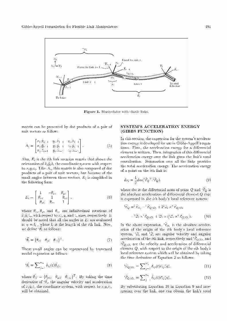
In this section, the kinematics of a chain of n elasticlinks is taken into consideration. The coordinatesystem of every link is attached according to the rulesdeveloped by Denavit and Hartenberg. X0Y0Z0 is thecoordinate system that is attached to the base of themanipulator and can be considered as the referencecoordinate system. Because of the elastic property ofthe links, two rotations occurred one of which is in thejoints and the other of which is in the links. It is usefulto separate the transformations due to the joints fromthe transformations which are due to the exible links.So, we allocate two coordinates system to each link.xiyizi is a coordinate system on link i whose origin islocated at the beginning of this link, but xiyizi is thecoordinate system that is attached to the end of thislink. When link i has no deformation, the axes of xiyiziare parallel to the axes of xiyizi .

In Figure 1, the arbitrary point, Q, is shown.The position of this point with respect to the ithbody's local reference system is expressed by i~rQ=Oi .To incorporate the de ection of the link, the approachof modal analysis is used. So:

i~rQ=Oi = ~� +Xmi

j=1�ij(t)~rij(�); (2)

where ~� = f� 0 0gT and ~rij = fxij yij zijgT . Also,� is the undeformed distance between the origin, Oi,and the point, Q; xij ; yij and zij are the displacementcomponents of j mode of the ith link; �ij is the timevarying amplitude of mode j of link i; and mi is thenumber of modes used to describe the de ection oflink i.

By using the rotation matrix, jRi, we can expressthe arbitrary vector, i~a, in every coordinate system, j,in the following form:

j~a = jRii~a: (3)

As noted above, it is better to separate the rotations,due to joints from de ections. So, jRi can be presentedrecursively as follows:

jRi = jRi�1Ei�1Ai; (4)

where Ai is the rotation matrix of the ith joint thatshows the orientation of the xiyizi coordinate systemwith respect to xi�1yi�1zi�1. The coe�cients of this

Gibbs-Appell Formulation for Flexible Link Manipulators 481

Figure 1. Manipulator with elastic links.

matrix can be presented by dot products of a pair ofunit vectors as follow:

Ai =

24xi:xi�1 yi:xi�1 zi:xi�1xi:yi�1 yi:yi�1 zi:yi�1xi:zi�1 yi:zi�1 zi:zi�1

35 : (5)

Also, Ei is the ith link rotation matrix that shows theorientation of xiyizi the coordinate system with respectto xiyizi. Like Ai, this matrix is also composed of dotproducts of a pair of unit vectors, but because of thesmall angles between these vectors, Ei is simpli�ed inthe following form:

Ei =

24 1 ��zi �yi�zi 1 ��xi��yi �xi 1

35 ; (6)

where �xi; �yi and �zi are in�nitesimal rotations ofxiyizi, with respect to xi; yi and zi axes, respectively. Itshould be noted that all the angles in Ei are evaluatedat � = li , where li is the length of the ith link. Now,we de�ne i~�i as follows:

i~�i = f�xi �yi �zigT : (7)

These small angles can be represented by truncatedmodal expansion as follows:

i~�i =Xmi

j=1�ij(t)~�ij ; (8)

where ~�ij = f�xij �yij �zijgT . By taking the timederivative of i~�i, the angular velocity and accelerationof xiyizi the coordinate system, with respect to xiyizi,will be obtained.

SYSTEM'S ACCELERATION ENERGY(GIBBS FUNCTION)

In this section, the expression for the system's accelera-tion energy is developed for use in Gibbs-Appell's equa-tions. First, the acceleration energy for a di�erentialelement is written. Then, integration of this di�erentialacceleration energy over the link gives the link's totalcontribution. Summation over all the links providesthe total acceleration energy. The acceleration energyof a point on the ith link is:

dsi =12dm(i�~rQT :i�~rQ); (9)

where dm is the di�erential mass of point Q and i�~rQ isthe absolute acceleration of di�erential element Q thatis expressed in the ith body's local reference system:

i�~rQ =i �~rOi +i �~rQ=Oi + 2i~!i �i _~rQ=Oi

+ i _~!i �i~rQ=Oi + i~!i � (i~!i �i ~rQ=Oi): (10)

In the above expression, i�~rOi is the absolute acceler-ation of the origin of the ith body's local referencesystem, i~!i and i _~!i are angular velocity and angularacceleration of the ith link, respectively and i _~rQ=Oi andi�~rQ=Oi are the velocity and acceleration of di�erentialelement Q, with respect to the origin of the ith body'slocal reference system which will be obtained by takingthe time derivative of Equation 2 as follows:

i _~rQ=Oi =Xmi

j=1_�ij(t)~rij(�); (11)

i�~rQ=Oi =Xmi

j=1��ij(t)~rij(�): (12)

By substituting Equation 10 in Equation 9 and inte-grating over the link, one can obtain the link's total


acceleration energy. In this paper, it is assumed thatthe links are slender beams. For slender beams, dm =�d� where � is mass per unit length. So, one canintegrate over � from 0 to li. Only the terms in i~rQ=Oiand its derivatives (i _~rQ=Oi ; i�~rQ=Oi) are functions of �for this link. Thus, the integration can be performedwithout knowledge of i~!i; i _~!i and i�~rOi . Summing overall n links, one �nds the system's acceleration energyto be:

S =Xn

i=1

Z li

0dsi

S =Xn

i=1

12Mi

i�~rOiT :i�~rOi + i�~rOi

T :i ~B1i

� 2i�~rOiTB2i

i~!i � i�~rOiTB3i

i _~!i � i�~rOiT i~!iB3i

i~!i

+12B4i � 2i~!iT :i ~B5i + i _~!Ti :

i ~B6i

� i~!iTB7ii~!i + 2i _~!iTB8i

i~!i +12i _~!iTB9i

i _~!i

+ i _~!iT i~!iB9ii~!i + irrelevant terms; (13)

where:

i ~B1i =Z li

0�i�~rQ=Oid�; (14)

B2i =Z li

0�i _~rQ=Oid�; (15)

B3i =Z li

0�i~rQ=Oid�; (16)

B4i =Z li

0�i�~rQ=Oi :

i�~rQ=Oid�; (17)

i ~B5i =Z li

0�i�~rQ=Oi

i _~rQ=Oid�; (18)

iB6i =Z li

0�i~rQ=Oi

i�~rQ=Oid�; (19)

B7i =Z li

0�i~rQ=Oi

T i�~rQ=Oid�; (20)

B8i =Z li

0�i~rQ=Oi

T i _~rQ=Oid�; (21)

B9i =Z li

0�i~rQ=Oi

T i~rQ=Oid�: (22)

In Equation 13, Mi is the total mass of the ith link.Also i~rQ=Oi , i _~rQ=Oi , i�~rQ=Oi and i~!i are skew-symmetric

tensors representation of the i~rQ=Oi ; i _~rQ=Oi ; i�~rQ=Oi andi~!i vectors. For developing an expression for S, thesevector relations, ~a:~b = ~b:~a, ~a �~b = ~a~b and (~a �~b):~c =~a:(~b � ~c) are frequently used. By interchanging theintegration and summation in Equations 14 to 22, oneobtains:

i ~B1i =Xmi

j=1��ij~"ij ; (23)

B2i =Xmi

j=1_�ij ~"ij ; (24)

B3i = gMirri +Xmi

j=1�ij ~"ij ; (25)

B4i =Xmi

j=1

Xmi

k=1��ij��iksCijk; (26)

i ~B5i =Xmi

j=1

Xmi

k=1��ij _�ik~cijk; (27)

i ~B6i =Xmi

j=1��ij~�ij ; (28)

B7i =Xmi

j=1��ij�ij ; (29)

B8i =Xmi

j=1_�ij�ij ; (30)

B9i = ci +Xmi

j=1�ijcijT +

Xmi

k=1�ik�ik; (31)

where:

~�ij = ~cij +Xmi

k=1�ik~cikj ; (32)

�ij = cij +Xmi

k=1�ikmcikj : (33)

By de�nition, ~� and ~rij are skew-symmetric tensorsassociated with ~� and ~rij vectors. The expressions of~"ij ; ~"ij ;gMirri ;

scijk;~cijk;~cij ; cij ;mcijk; ci that appearedin Equations 23 to 33 can be written in the followingform:

~"ij =Z li

0�~rijd�; (34)

~"ij =Z li

0�~rijd�; (35)

gMirri =Z li

0�~�d�; (36)


scijk =Z li

0�~rijT~rikd�; (37)

~cijk =Z li

0�~rij~rikd�; (38)

~cij =Z li

0�~�~rijd�; (39)

cij =Z li

0�~� T ~rijd�; (40)

mcijk =Z li

0�~rijT ~rikd�; (41)

ci =Z li

0�~�T ~�d�: (42)

Now, it should be noted that B9i has a unit of inertiamatrix. For example, its �rst term (ci) represent rigid-body-inertia terms. It can also be shown that mcijk =mcikjT . The terms de�ned in Equations 23 to 33 areeasily simpli�ed if one link in the system is consideredrigid (mi = 0). Furthermore, the expression for B9ihas a term of order �2, which is small and a candidatefor later elimination [5]. Finally, the integration of themodal shape products in Equations 34 to 42 can bedone o�-line one time for a given link structure.

Derivatives of Acceleration Energy

G-A equations are obtained by taking the derivative ofGibbs' function, with respect to generalized accelera-tions (�qj ; ��jf ):

@S@�qj

;@S@��jf

:

In Equation 13, there was a term named an irrelevantterm. In fact, in Gibbs' function, the terms that arenot functions of �qj and ��jf can be eliminated, becausethey have no role in construction of the derivative ofacceleration energy.

In Gibbs' function, only i�~rOi and i _~!i are functionsof �qj . So, the partial derivative of Gibbs' function withrespect to �qj becomes:

@S@�qj

=Xn

i=j+1

@i�~rOiT

@�qj

�Mi

i�~rOi + i ~B1i

� 2B2ii~!i �B3i

i _~!i � i~!iB3ii~!i�

+Xn

i=j

@i _~!iT

@�qj

�B3i

i�~rOi + i ~B6i

+ 2B8ii~!i +B9i

i _~!i + i~!iB9ii~!i�: (43)

Here, it should be noted that, in the above expres-sion, this property of the skew-symmetric matrix, inwhich aT = �a is used. The partial derivative ofGibbs' function with respect to ��jf is more complex,because in addition to i�~rOi and i _~!i, the expressionsof i ~B1i; B4i; i ~B5i; i ~B6i and B7i are also functions ofde ection variables. So, the expression of @S

@��jfcan be

presented as follows:

@S@��jf

=Xn

i=j+1

@i�~rOiT

@��jf

�Mi

i�~rOi + i ~B1i

� 2B2ii~!i �B3i

i _~!i � i~!iB3ii~!i )

+Xn

i=j+1

@i _~!iT

@��jf

�B3i

i�~rOi + i ~B6i

+ 2B8ii~!i +B9i

i _~!i � i~!iB9ii~!i )

+Xmj

k=1��jkscjfk � 2j~!jT

Xmj

k=1_�jk~cjfk

� j~!jT�jf j~!j + j�~rOjT~"jf + j _~!jT ~�jf : (44)

An additional simpli�cation of @S@��jf

arises, due to thefact that scjfk = scjkf .

SYSTEM'S POTENTIAL ENERGY

The potential energy of the system arises from twosources:

1. Potential energy due to gravity,2. Potential energy due to elastic deformations.

The e�ect of gravity on manipulators can beconsidered simply by putting 0�~rO0 = ~g, where ~g is theacceleration of gravity. Under these circumstances, wecan assume that the base of the manipulator has anacceleration of 1 g to the top. So, the e�ect of gravityhas been considered without additional computations.

To express the strain potential energy stored inthe ith link, let us assume that the assumptions ofthe classical beam (Euler-Bernoulli) hold. So, thestrain potential energy will be expressed in terms ofde ections and rotations as follows:

Vei =12

Z li

0

"EA

�@ui@�

�2

+ EIy�@2wi@�2

�2

+ EIz�@2vi@�2

�2

+GIx�@�xi@�

�2#d�; (45)

where EIy and EIz are the bending sti�ness in the OYand OZ directions, respectively; EA is the extensional


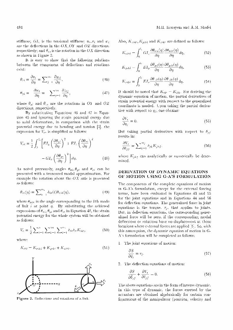
sti�ness; GIx is the torsional sti�ness; ui; vi and wiare the de ections in the OX;OY and OZ directions,respectively; and �xi is the rotation in the OX directionas shown in Figure 2.

It is easy to show that the following relationsbetween the component of de ections and rotationsexist:

�zi =@vi@�

=Xmi

j=1

@yij@�

; (46)

�yi = �@wi@�

= �Xmi

j=1

@zij@�

; (47)

where �yi and �zi are the rotations in OY and OZdirections, respectively.

By substituting Equations 46 and 47 in Equa-tion 45 and ignoring the strain potential energy dueto axial deformation, in comparison with the strainpotential energy due to bending and torsion [5], theexpression for Vei is simpli�ed as follows:

Vei =12

Z li

0

�EIy

�@�yi@�

�2

+ EIz�@�zi@�

�2

+GIx�@�xi@�

�2 �d�: (48)

As noted previously, angles �xi; �yi and �zi can bepresented with a truncated modal approximation. Forexample the rotation about the OX axis is presentedas follows:

�xi(�) =Xmi

k=1�ik(t)�xik(�); (49)

where �xik is the angle corresponding to the kth modeof link i at point �. By substituting the achievedexpressions of �xi; �yi and �zi in Equation 48, the strainpotential energy for the whole system will be obtainedas follows:

Ve =12

Xn

i=1

Xmi

k=1

Xmi

l=1�ik�ilKikl; (50)

where:

Kikl = Kxikl +Kyikl +Kzikl: (51)

Figure 2. De ections and rotations of a link.

Also, Kxikl;Kyikl and Kzikl are de�ned as follows:

Kxikl =Z li

0GIx

@�xil(�)@�

@�xik(�)@�

d�; (52)

Kyikl =Z li

0EIy

@�yil(�)@�

@�yik(�)@�

d�; (53)

Kzikl =Z li

0EIz

@�zil(�)@�

@�zik(�)@�

d�: (54)

It should be noted that Kikl = Kilk. For deriving thedynamic equation of motion, the partial derivatives ofstrain potential energy with respect to the generalizedcoordinate is needed. Upon taking the partial deriva-tive with respect to qj , one obtains:

@Ve@qj

= 0: (55)

But taking partial derivatives with respect to �jfresults in:

@Ve@�jf

=Xmj

k=1�jkKjkf ; (56)

where Kjkf can analytically or numerically be deter-mined.

DERIVATION OF DYNAMIC EQUATIONSOF MOTION USING G-A'S FORMULATION

The components of the complete equations of motionin G-A's formulation, except for the external forcingterms, have been evaluated in Equations 43 and 55for the joint equations and in Equations 44 and 56for de ection equations. The generalized force in jointequations is the torque, �j , that applies to joints.But, in de ection equations, the corresponding gener-alized force will be zero, if the corresponding modalde ections or rotations have no displacement at thoselocations where external forces are applied [5]. So, withthis assumption, the dynamic equation of motion in G-A's formulation will be completed as follows:

1. The joint equations of motion:

@S@�qj

= �j : (57)

2. The de ection equations of motion:

@S@��jf

+@Ve@�jf

= 0: (58)

The above equations are in the form of inverse dynamic.In this type of dynamic, the forces exerted by theactuators are obtained algebraically for certain con-�gurations of the manipulator (position, velocity and


acceleration). On the other hand, the forward dynamicproblem computes the acceleration of the joints of themanipulator, once the forces exerted by the actuatorsare given. This problem is part of the process that mustbe followed to perform the simulation of the dynamicbehavior of the manipulator. This process is completedafter it calculates the velocity and position of thejoints by means of a process of numerical integrationin which the acceleration of the joints and the initialcon�guration are data input to the problem [15].

FORWARD DYNAMIC EQUATIONS OFMOTION

In this section, the �rst step will extend the equationsof i�~rOi and also i _~!i. These equations are used toseparate the second derivatives of joint variables andde ection variables from the dynamic equations ofmotion.

The absolute acceleration of the origin of the ithbody's local reference system in recursive form can bepresented as follows:

i�~rOi = iRi�1

�i�1�~rOi�1 + i�1�~rOi=Oi�1 + 2i�1~!i�1

� i�1 _~rOi=Oi�1 + i�1 _~!i�1 � i�1~rOi=Oi�1

+ i�1~!i�1 � �i�1~!i�1 � i�1~rOi=Oi�1

��; (59)

where:

i~rOi+1=Oi = ~li +Xmi

j=1�ij(t)~rij(li); (60)

i _~rOi+1=Oi =Xmi

j=1_�ij(t)~rij(li); (61)

i�~rOi+1=Oi =Xmi

j=1��ij(t)~rij(li); (62)

and also ~li = fli 0 0gT . Before developing anexpression for angular acceleration, we should presentangular velocity, because by taking its time derivative,angular acceleration will be obtained. The angularvelocity of the ith link is the same as the i � 1th linkplus two new components, one of which (i~zi _qi), comesfrom the angular velocity of the ith link and the other(i�1 _~�i�1) is produced due to the elasticity of the i�1thlink. So, the expression of angular velocity can bepresented as follows:

i~!i = iRi�1

�i�1~!i�1 +i�1 _~�i�1(li�1)

�+ i~zi _qi; (63)

where:

i _~�i(li) =Xmi

j=1_�ij(t)~�ij(li); (64)

and i~zi = f0 0 1gT . By taking the time derivative ofEquation 63, the expression of angular acceleration willbe obtained:

i _~!i= iRi�1

�i�1 _~!i�1+i�1 �~�i�1+i�1~!i�1 � i�1 _~�i�1

�+ iRi�1

�i�1~!i�1 + i�1 _~�i�1

�� i~zi _qi + i~zi�qi: (65)

In the above expression, i�1 �~�i�1(li�1) is the angularacceleration that is produced because of the elasticityof the i� 1th link:

i�~�i (li) =Xmi

j=1��ij (t) ~�ij (li): (66)

Now, by having i�~roi and i _~!i in recursive form, we canconvert them in summation form as follows:

i�~rOi =Xi�1

k=1iRkk�~rOk+1=Ok

+Xi�1

k=1iRk

�k _~!k � k~rOk+1=Ok

�+ i�~rOv;i ; (67)

i _~!i =Xi

k=1iRkk~zk�qk

+Xi�1

k=1iRkk

�~�k (lk) + i _~!v;i; (68)

where:

i�~rOv;i = 2Xi�1

k=1iRk

�k~!k � k _~rOk+1=Ok

�+Xi�1

k=1iRk

�k~!k � �k~!k � k~rOk+1=Ok��; (69)

i _~!v;i =Xi�1

k=1iRkk~!k � iRk+1

k+1~zk+1 _qk+1

+Xi�1

k=1iRkk

_~�k � iRk+1k+1~zk+1 _qk+1: (70)

In fact, i�~rov;i and i _~!v;i are those constructive terms ofi�~roi and i _~!i that do not contain the second derivativesof joint variables and de ection variables. By havingi�~roi and i _~!i in summation form, the calculation of par-tial derivatives that appeared in the dynamic equationsof motion can be done as follows:

@i _~!i@�qj

= iRjj~zj ; (71)

@i _~!i@��jf

= iRj~�jf (lj); (72)

@i�~rOi@�qj

= iRjj~zj � i~rOi=Oj ; (73)


@i�~rOi@��jf

= iRj~rjf (lj) + iRj~�jf (lj)� i~rOi=Oj+1 ; (74)

where i~roi=oj is a position vector drawn from the jthbody's local reference system to the ith body's localreference system (j < i).

Inertia Coe�cients

For construction of the inertia coe�cients that multiplythe second derivatives, we substitute Equations 71 to74 and also the summation form of i�~roi and i _~!i (Equa-tions 67 to 68) into the relevant parts of Equations 43and 44. By collecting the terms that contain �qj and��jf and by arranging them, we obtain expressions thatshould be written in matrix form. By assembling thesematrixes, the inertia matrix of the whole system willbe obtained. In continuation the details of the abovesteps are brought.

Inertia Coe�cients of Joint Variable in JointEquationsAll occurrences of �qj in Equation 43 are in the ex-pressions of i _~!i and i�~roi ; by isolating these terms andinterchanging the order of summations as follows:

nXi=j

Xi

k=1=n�1Xk=1

Xn

i=max(k+1;j);

nXi=j+1

Xi

k=1=

nXk=1

Xn

i=max(k;j+1);

nXi=j

Xi�1

k=1=n�1Xk=1

Xn

i=max(k+1;j);

nXi=j+1

Xi�1

k=1=n�1Xk=1

Xn

i=max(k+1;j+1);

n�1Xk=1

Xk

t=1=n�1Xt=1

Xn�1

k=t;

the below expression for the terms that contain �qj isobtained:�Xn

k=1j~zjT (j�k�j k)k~zk �Xn�1

k=1j~zjT jUkk~zk

��qk;(75)

where:

j�k =nX

i=max(k;j)

jRiB9iiRk; (76)

j k =nX

i=max(k;j+1)

j~rOi=OjjRiB3i

iRk; (77)

jUk =n�1Xt=k

(j t + j�t+)t~rOt+1=OttRk: (78)

Also j t and j�t+ are de�ned as follows:

j t =nX

i=max(t+1;j+1)

j~rOi=OjMijRt; (79)

j�t+ =nX

i=max(t+1;j)

jRiB3iiRt: (80)

In the next section, Expression 75 will be written inmatrix form that makes the inertia matrix of the jointvariable in the joint equations. As will be shown, thismatrix is symmetric and this fact reduces the necessarycomputations. Also, the expressions appeared in sum-mation form (j�t+ ; j t; jUk; j k; j�k) can be calculatedrecursively. This is an important issue that causesthe reduction of necessary computations and will beconsidered in detail in the next section.

Inertia Coe�cients of De ection Variables inJoint EquationsIn consideration of Equation 43, we observe that thede ection variables ��jf appear not only in i�~rOi and i _~!i,but also in i ~B1i and i ~B6i. By isolating these terms, theexpression for the terms that contain ��jf is obtained asbelow:�Xn�1

k=1

Xmk

t=1j~zjT

�j�k+ � j k+� ~�kt

+Xn�1

k=1

Xmk

t=1j~zjT

�j�k+ + j k�~rkt

�Xn�2

k=1

Xmk

t=1j~zjT jUk+~�kt

+Xn

k=j+1

Xmk

t=1j~zjT j~rOk=Oj

jRk~"kt

+Xn

k=j

Xmk

t=1j~zjT jRk~�kt

��kt; (81)

where:

j�k+ =nX

i=max(k+1;j)

jRiB9iiRk; (82)

j k+ =nX

i=max(k+1;j+1)

j~rOi=OjjRiB3i

iRk; (83)


jUk+ =n�1Xt=k+1

�j t + j�t+� t~rOt+1=Ot

tRk: (84)

By writing Expression 81 in matrix form, the inertiacoe�cients of de ection variables in the joint equationswill be obtained.

It can be shown that the inertia coe�cients forjoint variables in the de ection equations are the sameas the coe�cients of de ection variables in the jointequations. This issue implies the symmetry of theinertia matrix of the whole system and can be usedfor reduction of necessary computations.

Inertia Coe�cients of De ection Variables inDe ection EquationsIn a manner much the same as the previous two steps,the below expression is obtained by isolating the termsthat contain ��jf in de ection equations:�Xn�1

k=1

Xmk

t=1~�jf T

�j+�k+ � j+ k+

�~�kt

�Xn�2

k=1

Xmk

t=1~�jf T j

+Uk+~�kt

�Xn�2

k=1

Xmk

t=1~rjf T jVk~�kt

�Xn�1

k=1

Xmk

t=1~rjf T j

+�k+~�kt

�Xj�2

k=1

Xmk

t=1~"jf T jWk~�kt

+Xj�1

k=1

Xmk

t=1~�jf T jRk~�kt +

Xmj

t=1scjft

+Xn�1

k=1

Xmk

t=1~�jf T

�j+ k + j+�k+

�~rkt

+Xn�1

k=1

Xmk

t=1~rjf T j�k~rkt

+Xj�1

k=1

Xmk

t=1~"jf T jRk~rkt

+Xn

k=j+1

Xmk

t=1~rjf T jRk~"kt

+Xn

k=j+2

Xmk

t=1~�jf T j~rOk=Oj+1

jRk~"kt

+Xn

k=j+1

Xmk

t=1~�jf T jRk~�kt

��kt; (85)

where:

j+�k+ =nX

i=max(k+1;j+1)

jRiB9iiRk; (86)

j+�k+ =nX

i=max(k+1;j+1)

jRiB3iiRk; (87)

jVk =n�1Xt=k+1

j�tt~rot+1=ottRk; (88)

j+ k+ =nX

i=max(k+1;j+2)

j~roi=oj+1jRiB3i

iRk; (89)

j+ k =nX

i=max(k+1;j+2)

j~roi=oj+1MijRk; (90)

jWk =j�1Xt=k+1

jRtt~rot+1=ottRk; (91)

j+Uk+ =n�1Xt=k+1

�j+ t + j+�t+

�t~rot+1=ot

tRk; (92)

j�k =nX

i=max(k+1;j+1)

MijRk: (93)

Like the previous two steps, the above expression iswritten in matrix form. The symmetry of this matrixcan be shown by expanding its coe�cients. On theother hand, all the expressions in summation form canbe calculated recursively.

Final Form of Forward Dynamic Equations

The complete simulation equations have now beenderived. It remains to assemble them in �nal formand point out some remaining recursions that can beused to reduce the number of calculations. The secondderivatives of the joint and de ection are desired onthe \left hand side" of the equation as unknowns,and the remaining dynamic e�ects and the inputs aredesired on the \right hand side". To carry out thisprocess completely, one would take the inverse of theinertia matrix, I(�) , and premultiply the vector ofother dynamic e�ects,

!Re. Because of its complexity,

this inverse can only be evaluated numerically. Thus,for the purpose of this paper, the equations will beconsidered in the following form:

I(�) �~� =!Re; (94)

where:

I(�) The inertia matrix consisting of coe�cientswill be obtained in the next section;


~� The vector of generalized coordinate;~� fq1 �11 �12 � � � �1m1 q2 �21 � � �

�2m2 � � � qk �k1 � � � �kmk � � � �nmngT ;qk The joint variable for the kth joint;�kt The de ection variable (amplitude) of

the tth mode of link k;!Re Vectors of remaining dynamics and external

forcing terms, f Re1 Re11 � � � Re1m1

Re2 Re21 � � � Re2m2 � � � Rej Rej1� � � Rejmj � � � RenmngT ;Rej Dynamics from the joint equations j

(Equation 43), excluding second derivativesof the generalized coordinate;

Rejf Dynamics from the de ection equations jf(Equation 44), excluding secondderivatives of the generalized coordinate.

At �rst, consider Rej . In joint equations, by collectingthe terms that do not contain �qj and ��jf , theexpression is obtained as below:

Rej=�j�Xn

i=j+1

@i�~rOiT

@�qj:i~Si�Xn

i=j

@i _~!iT

@�qj:i ~Ti;

(95)

where:

i~Si = Mii�~rOv;i � 2B2i

i~!i �B3ii _~!v;i � i~!iB3i

i~!i;(96)

i ~Ti = B3ii�~rOv;i + 2B8i

i~!i +B9ii _~!v;i + i~!iB9i

i~!i:(97)

By substituting Equations 71 and 73 in Equation 95and changing it to a recursive expression, a newequation for Rej is obtained:

Rej = �j � j~zjT j~�j ; (98)

where:

j~�j = j ~Tj + j~rOj+1=Ojj~�j + jRj+1

j+1~�j+1; (99)

and:

j~�j = jRj+1

�j+1~Sj+1 + j+1~�j+1

�: (100)

Now, consider Rejf . If in the defection equation theterms that do not contain �qj and ��jf are collected, thefollowing expression will be obtained:

Rejf =�Xmi

k=1�jkKjkf �Xn

i=j+1

@i�~rOiT

@��jf:i~Si

�Xn

i=j+1

@i _~!iT

@��jf:i ~Ti +Qjf ; (101)

where:

Qjf = 2j!jT :Xmj

k=1_�jk~cjfk + j~!jT�jf j~!j

� j�~rov;jT :~"jf � j _~!v;jT � ~�jf : (102)

Like the previous step, the following recursive equationfor Rejf is obtained:

Rejf =�Xmj

k=1�jkKjkf +Qjf

� ~rjf T :j~�j � ~�jf T jRj+1j+1~�j+1: (103)

Equations 98 and 103 are used to construct the righthand side equations of motion.

PROPOSED ALGORITHM

Now, we shall present an algorithm that results fromthe expressions developed in previous sections. Inthis algorithm, all cross products are done in tensornotation. And, also, each speci�c algorithmic ex-pression is accompanied by information that indicatesthe number of algebraic operations that are involved,showing separately products M and A sums. Thecalculations are done in a step by step process, asfollows:

Step 1: The rotation matrix will be calculated by thisalgorithm.

for i = 2 : 1 : n

i�1Ri = Ei�1Ai & iRi�1 = i�1RiT ; 15M6A

Step 2: The vectors of i~!i, i _~!v;i and i�~rOv;i can becalculated recursively, as follows.

Initialize:

1~!1 = 1~z1 _q1; & 1 _~!v;1 = f0 0 0gT ; &

1�~rOv;1 = A1T fgx gy gzgT ;

for i = 2 : 1 : n

Equation 63 9M10A

i _~!v;i = iRi�1

��i�1 ~!i�1 + i�1 _~�i�1

�i�1Rii~zi _qi

+ i�1 _~!v;i�1

�; 18M18A


i�~rov;i = iRi�1

�2i�1 ~!i�1

i�1 _~roi=oi�1

+ i�1 _~!v;i�1i�1~roi=oi�1

+ i�1 ~!i�1�i�1 ~!i�1

i�1~roi=oi�1

�+i�1�~rov;i�1 ) ; 33M27A

Step 3: In this step, the vectors of i~Si and i ~Ti arecalculated.

for i = 2 : 1 : n

Equation 96; 27M 21A

for i = 1 : 1 : n


Step 4: The vectors of i~�i and i~�i can be calculatedby the following algorithm:

Initialize:

n~�n = f0 0 0gT ; & n~�n = n ~Tn

for j = n� 1 : �1 : 1

Equation 100; 9M 9A


Step 5: Calculation of Qjf ,

for j = 1 : 1 : n; f = 1 : 1 : mj


Step 6: In this step, Equations 98 and 103 are usedto calculate Rej and Rejf .

for j = 1 : 1 : n

Equation 98; 0M 1A

for f = 1 : 1 : mn

Renf = �Xmn

k=1�nkKnkf +Qnf ; 0M 1A

for j = 1 : 1 : n� 1; f = 1 : 1 : mj


At the end of this step, the right hand side ofthe equations of motion is completely evaluated. Incontinuation, a recursive algorithm is presented thatevaluates the left hand side of the equations of motion

and, also, the inertia matrix of the whole system.

Step 7: Calculation of the compound rotation matrix,

for j = 1 : 1 : n

jRj = I3�3;

for j = 1 : 1 : n� 2; k = j + 2 : 1 : n

jRk = jRk�1k�1Rk; &

kRj = jRkT ; 27M 18A

Step 8: The following algorithm evaluates the vectorof i~rOj=Oi :

for j = 2 : 1 : n� 1; j = i� 1 : �1 : 1

j~rOi+1=Oi = jRj+1j+1~rOi+1=Oi ; 9M 6A

for i = 1 : 1 : n� 2; j = i+ 2 : 1 : n

i~rOj=Oi = i~rOj�1=Oi + i~rOj=Oj�1 ; 0M 3A

Step 9: In this step, the variables that have beenappeared in summation form in the inertia matrix areevaluated.

� Calculation of j�k:

for k = n : �1 : 1; j = k : �1 : 1

if (k = j)

if (k = n) n�n = B9n;

else

k�k = B9k + k�k+1k+1Rk; 27M 27A

else

j�k= jRj+1j+1�k; & k�j= j�kT ; 27M 18A

A recursive algorithm, like the one mentionedabove, for calculation of j�k, can be used. However,it should be noticed that, instead of B9i , we haveB3i and, also, at the last line, we have:

k�j = �j�kT ;

� Calculation of j k:

for j = n� 1 : �1 : 1

j n = j~rOn=Ojj�n; 18M 9A


for j = n� 1 : �1 : 1; k = n� 1 : �1 : 1

if (k > j)

j k= j k+1k+1Rk + j~rOk=Oj

jRkB3k; 63M 45A

else j k = j k+1k+1Rk; 27M 18A

� Calculation of j�k:

for k = n� 1 : �1 : 1; j = k : �1 : 1

if (k = j)

if (k = n� 1) n�1�n�1 = MnI3�3; 3M 0A

else

k�k = Mk+1I3�3 + k+1�k+1; 3M 3A

else

j�k= jRj+1j+1�k; & k�j= j�kT ; 27M 18A

� Calculation of j k:

for j = n� 1 : �1 : 1

j n�1 = j~rOn=Ojj�n�1; 18M 9A

for j = n� 1 : �1 : 1; k = n� 2 : �1 : 1

if(k < j) j k = j k+1k+1Rk; 27M 18A

else

j k= j k+1k+1Rk+Mk+1

j~rOk+1=OjjRk; 51M 36A

� Calculation of jUk:

for j = 1 : 1 : n

jUn�1 =�j n�1 + j�n�1+

� n�1~rOn=On�1 ;

18M 18A

for j = 1 : 1 : n; k = n� 2 : �1 : 1

jUk =�j k + j�k+

� k~rOk+1=Ok

+ jUk+1k+1Rk; 45M 45A

� Calculation of jVk:

for j = 1 : 1 : n� 1

jVn�2 = j�n�1n�1~rOn=On�1

n�1Rn�2; 18M 9A

for j = 1 : 1 : n� 1; k = n� 3 : �1 : 1

jVk = j�k+1k+1~rOk+2=Ok+1

k+1Rk

+ jVk+1k+1Rk; 45M 36A

� Calculation of j�k+ :

for k = 1 : 1 : n� 1; j = 1 : 1 : n

j�k+ = j�k+1k+1Rk; 27M 18A

� Calculation of j+�k+ :

for j = 1 : 1 : n� 1; k = 1 : 1 : n� 1

j+�k+ = jRj+1j+1�k+ ; 27M 18A

For calculation of j�k+ ; j k+ and jUk+ we use thealgorithm like the one that was used for calculationof j�k+ . Also, j

+�k+

j+ k+j+ k and j+Uk+ can be

calculated by the algorithm like the one that wasused for calculation of j

+�k+ .

Step 10: Finally, calculation of the inertia matrix forthe whole system is considered.

� Calculation of the inertia matrix for joint variablesin joint equations:

for j = 1 : 1 : n� 1; k = j : 1 : n� 1

Ijk = j~zjT�j�k � j k � jUk

� k~zk; &

Ikj = Ijk; 0M 18A

for j = 1 : 1 : n

if (j 6= n) Ijn= j~zjT�j�n � j n

� n~zn; &

Inj = Ijn; 0M 9A

else Inn = n~znT n�nn~zn; 0M 0A


� Calculation of the inertia matrix for de ection vari-ables in joint equations:

for j = 2 : 1 : n; k = 1 : 1 : j � 1; t = 1 : 1 : mk

Ijkt = j~zjT��j�k+ � j k+ � jUk+

� ~�kt+�j�k+ + j k

�~rkt ) ; 18M 42A

for j = 1 : 1 : n� 1; k = j; t = 1 : 1 : mk


� ~�kt+�j�k+ + j k

�~rkt + ~�kt ) ; 18M 45A

for j=1 : 1 : n� 2; k=j+1 : 1 : n�1; t=1:1:mk


� ~�kt+�j�k+ + j k

�~rkt + jRk~�kt

+ j~rOk=OjjRk~"kt ) ; 42M 63A

for j=1 : 1 : n� 1; k=n; t=1 : 1 : mk

Ijnt = j~zjT�jRk~�kt + j~rOk=Oj

jRk~"kt�

; 24M 18A

for j = k = n; t = 1 : 1 : mk

Ijkt = j~zkT ~�kt; 0M 0A

� Calculation of de ection variables in de ection equa-tions:

for j=1 : 1 :n� 1; k=j; t=1 : 1: mk; f=1 : 1:mj

Ijkft = ~�jf T�j+ k + j+�k+

�~rkt

+�j+�k+ � j+ k+ � j+Uk+

�~�kt

� ~rjf T��

jVk + j+�k+

�~�kt � j�k~rkt

�+ scjft; 42M 72A

for j=1 : 1: n�2; k=j+1 : 1 : n�1; t=1 : 1: mk;

f=1 : 1 : mj

Ijkft = ~�jf T��

j+ k + j+�k+

�~rkt

+�j+�k+ � j+ k+ � j+Uk+

�~�kt

+jRk~�kt + jRj+1j+1~rOk=Oj+1

j+1Rk~"kt )

�~rjf T��

jVk + j+�k+

�~�kt

� j�k~rkt � jRk~"kt�

; 84M 107A

for j=1 : 1 : n�1; k=n; t=1 : 1 : mk; f=1 : 1;mj

Ijkft= ~�jf T�jRk~�kt+jRj+1

j+1~rOk=Oj+1j+1Rk~"kt

�+~rjf T jRk~"kt; 48M 35A

for j = n; k = n; t = 1 : 1 : mk; f = 1 : 1 : mj

Ijfkt = scjft; 0M 0A

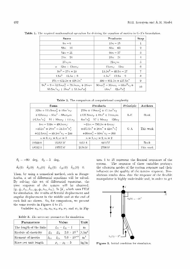
The required mathematical operations for calculatingthe above steps are listed in Table 1, where n is thetotal number of links; nf is the number of exible linksand m is the number of modes describing each exiblelink, the same for all exible links.

In Table 2, the computational complexity of thismethod compared with the ones of [5], are shown. Also,Table 2 shows the number of operations for two typicalcases.

As a general comparison, the number of mathe-matical operations of the method proposed in this ar-ticle for the dynamic modeling of exible manipulatorsis less than the recursive Lagrangian method in [5].

COMPUTATIONAL SIMULATION

In this section, we verify the proposed method forthe dynamic modeling of exible robotic manipulatorsin the preceding sections by means of computationalsimulation for a manipulator with two elastic links.The �rst mode shape of clamped-free beams is used tomodel the elastic deformation of each link. All neces-sary parameters of exible links for this computationalsimulation are shown in Table 3. These parameters arethe same as in [4].

To clearly explain computational procedures forthe simulation, we rewrite Equation 94 in state form.

_~�1 = ~�2;

_~�2 = I�1(�1)!Re:

The initial conditions are also the same as in [4] asshown in Figure 3.


Table 1. The required mathematical operation for deriving the equation of motion in G-A's formulation.

Sums Products Step

6n� 6 15n� 15 1

55n� 55 60n� 60 2

54n� 21 66n� 27 3

24n� 24 24n� 24 4

17nfm 21nfm 5

n� 12m+ 13mnf 15mnf � 15m 6

9n2 � 27n+ 18 13:5n2 � 40:5n+ 27 7

4:5n2 � 13:5n+ 9 4:5n2 � 13:5n+ 9 8

276� 652:5n+ 328:5n2 390� 901:5n+ 457:5n2 99n2 � 9 + 52:5mn2

f � 79:5mnf + 18m�89:5m2nf + 18m2 + 53:5m2n2

f

30mn2f � 30mnf � 60m2nf+18m2 + 42m2n2

f10

Table 2. The comparison of computational complexity.

Sums Products Principle Authors

329n+ 115:5mn2f + 19m2nf 279n+ 118mn2

f + 17:5m2nf+123mnf + 85n2 + 68nnfm +137:5mnf + 84n2 + 74nnfm L-E Book

+6:5m2n2f � 91 + 80nnf + 111nf +6m2n2

f � 57 + 86nnf + 126nf6m� 553n� 49:5mnf �15m� 790:5n+ 6mnf

+351n2 + 18m2 + 53:5m2n2f +475:5n2 + 18m2 + 42m2n2

f G-A This work+52:5mn2

f � 89:5m2nf + 188 +30mn2f � 60m2nf + 300

n = 6; nf = 6;m = 3 n = 3; nf = 2;m = 2

24569A 25251M 4851A 4922M Book

18332A 19557M 2134M 2706M This work

�1 = �90 deg; �2 = 5 deg;

_�1(0)= _�2(0)=�11(0)= _�12(0)=�21(0)= _�21(0)=0:

Then, by using a numerical method, such as Runge-Kutta, a set of di�erential equations will be solved.By solving this set of di�erential equations, thetime response of the system will be obtained,(q1; _q1; �11; _�11; q2; _q2; �21; _�21). In [4], which uses FEMfor simulation, the results of exural displacement andangular displacement in the middle and at the end ofeach link are shown. So, for comparison, we presentthe same results in Figures 4 to 15.

Variables u3; u4; u5; u6; w3; w4; w5 and w6 in Fig-

Table 3. The necessary parameters for simulation.

Parameters Value UnitThe length of the links L1 = L2 = 1 mModule of elasticity E1 = E2 = 2:0� 1011 N/m2

Moment of inertia I1z = I2z = 5:0� 10�9 m4

Mass per unit length �1 = �2 = 5 kg/m

ures 4 to 15 represent the exural responses of thesystem. The response of these variables portraysthe vibration modes of the system response and theirin uence on the quality of the system response. Sim-ulations results show that the response of the exiblemanipulator is highly undesirable and, in order to get

Figure 3. Initial condition for simulation.


Figure 4. Angular displacement of the �rst joint.

Figure 5. Angular displacement of the second joint.

Figure 6. X position of end e�ector.

Figure 7. Y position of end e�ector.

Figure 8. Flexural displacement in the middle of the �rstlink.

Figure 9. Flexural displacement at the end of the �rstlink.


Figure 10. Angular displacement in the middle of the�rst link.

Figure 11. Angular displacement at the end of the �rstlink.

Figure 12. Flexural displacement in the middle of thesecond link.

Figure 13. Flexural displacement at the end of thesecond link.

Figure 14. Angular displacement in the middle of thesecond link.

Figure 15. Angular displacement at the end of thesecond link.


the dynamics of the system to be acceptable for mostpractical purposes, very e�ective controls are neededto control the vibration modes. On the other hand,as seen, the results are in good concordance with onesin [4]. It should be noted that the simulation is doneby using only one mode shape. More accurate resultswill be obtained by using more mode shapes.

CONCLUSION

This article has presented an e�cient and systematicmethod for the dynamic modeling of exible roboticmanipulators. The proposed method can be appliedto the design of control systems and the dynamicsimulation of exible manipulators. The advantages ofthis method in comparison with others are as follows:

1. A reduction in computations by using only 3 � 3and 3� 1 matrices.

2. Increase in the speed of generating the equationsof motion by reducing the number of additions andmultiplications, as shown in Table 2.

3. Ease of understanding, as it uses primitive dynamicconcepts.

REFERENCES

1. Walker, M.W. and Orin, D.E. \E�cient dynamiccomputer simulation of robotic mechanisms", ASMEJ. Dynamic systems Meas. Control., 104, pp. 205-211(1982).

2. Megahed, S. and Renaud, M. \Minimization of thecomputation time necessary for the dynamic controlof robot manipulators", Proc. of the 12th ISIR, pp.469-478 (1982).

3. Vukobratovic, M., Li, S.G. and Kircanski, N. \Ane�cient procedure for generating dynamic manipulatormodels", Robotica., 3, pp. 147-152 (1985).

4. Usoro, P.B., Nadira, R. and Mahil, S.S. \A �niteelement / Lagrange approach to modeling lightweight exible manipulators", ASME J. Dynamic SystemsMeas. Control., 108, pp. 198-205 (1986).

5. Book, W.J. \Recursive Lagrangian dynamics of exiblemanipulator arms", Int. J. Robotics. Res., 3, pp. 87-101 (1984).

6. King, J.O., Gourishankar, V.G. and Rink, R.E. \La-grangian dynamics of exible manipulators using an-gular velocities instead of transformation matrices",

IEEE Trans. System Man Cybernet, SMC 17, pp.1059-1068 (1987).

7. Jin, C. and Sankar, T.S. \A systematic Method ofdynamics for exible robot manipulators", J. DynamicSystem., 9(7), pp. 861-891 (1992).

8. Korayem, M.H., Yau, Y. and Basu, A. \Applicationof symbolic manipulation to inverse dynamics andkinematics of elastic robot", International Journal ofAdvanced Manufacturing Technology, 9(4), pp. 343-350(1994).

9. Korayem, M.H. and Basu, A. \Automated fast sym-bolic modeling of robotic manipulators with compliantlink", International Journal of Scienti�c Computing &Modeling, 22(9), pp. 41-55 (1995).

10. Anderson, K.S. \An e�cient formulation for the mod-eling of general multi- exible-body constrained sys-tems", International Journal of Solids and Structures,30(7), pp. 921-945 (1993).

11. Banerjee, A.K. \Block-diagonal equations for multi-body elastodynamics with generic sti�ness and con-straints", AIAA Journal of Guidance, Control andDynamics, 16(6), pp. 1092-1100 (1993).

12. Dwivedy, S.K. and Eberhard, P. \Dynamic analysis of exible manipulators, a literature review", J. Mecha-nism and Machine Theory, 41(7), pp. 749-777 (2006).

13. Baruh, H., Analytical Dynamics, New York, McGraw-Hill (1998).

14. Vukobratovic, M. and Potkonjak, V., Applied Dynam-ics and CAD of Manipulation Robots, Springer-Verlag,Berlin (1985).

15. Desoyer, K. and Lugner, P. \Recursive formulation forthe analytical or numerical application of the Gibbs-Appell method to the dynamics of robots", Robotica.,7, pp. 343-347 (1989).

16. Vereshchagin, A.F. \Computer simulation of the dy-namics of complicated mechanisms of robotic manipu-lators", Eng. Cyber., 6, pp. 65-70 (1974).

17. Rudas, I. and Toth, A. \E�cient recursive algorithmfor inverse dynamics", Mechatronics., 3(2), pp. 205-214 (1993).

18. Mata, V., Provenzano, S., Cuadrado, J.I. and Valero,F. \Serial-robot dynamics algorithms for moderatelylarge number of joints", J. Mechanism and MachineTheory, 37, pp. 739-755 (2002).

Motion Equations Proper for Forward Dynamics of Robotic Manipulator … · 2017-11-28 · algorithm...

Documents

Transcript of Motion Equations Proper for Forward Dynamics of Robotic Manipulator … · 2017-11-28 · algorithm...