Portland State University Portland State University

PDXScholar PDXScholar

University Honors Theses University Honors College

2015

MOSCAP Oxide Charges MOSCAP Oxide Charges

August George Portland State University

Follow this and additional works at: https://pdxscholar.library.pdx.edu/honorstheses

Let us know how access to this document benefits you.

Recommended Citation Recommended Citation George, August, "MOSCAP Oxide Charges" (2015). University Honors Theses. Paper 139. https://doi.org/10.15760/honors.189

This Thesis is brought to you for free and open access. It has been accepted for inclusion in University Honors Theses by an authorized administrator of PDXScholar. For more information, please contact pdxscholar@pdx.edu.

MOSCAP Oxide Charges

by

August George

An undergraduate honors thesis submitted in partial fulfillment of the

requirements for the degree of

Bachelor of Science

in

University Honors

and

Physics

Thesis Adviser

Dr. Rajendra Solanki

Portland State University

2015

Table of Contents

Introduction….……………………………………………………………………………………….1

1.1 Introduction to Solid State Physics………………………………………………..…2

1.2 Semiconductors…………………………………………………………………………….…4

1.3 Doping………………………………………………………………………………………….….6

2.1 Wafer Fabrication………..……….…………………………………………………….……7

2.2 Impurities and Gettering………………………………………………………………….8

2.3 Oxide Growth……………………………………………………………………………..…….9

3.1 Material Interfaces…………………………………………………………………………11

3.2 MOSCAP Interface Characteristics………………………………………………….13

3.3 MOSCAP CV Curve Characteristics………………………………………….………13

4.1 Oxide Charges………………………………………………………………………………..16

Methods…………………………………………………………………………………..…………..17

Results and Discussion…………………………………………………………………..……19

Conclusion…………………………………………………………………………………………...20

Recommendations…………………………………………………………………………….…20

Acknowledgements………………………………………………………………..……………21

Appendix A – Wafer Fabrication Data Sheet………………………………….……..22

References………………………………………………………………………………………..…24

Abstract

Transistors form the backbone of digital devices, allowing for amplification

and digital “switching” of electrical signals. One of the simplest devices is the Metal-

Oxide-Semiconductor Capacitor (MOSCAP). The MOSCAP is analogous to a parallel

plate capacitor with the Si wafer and metal layer corresponding to the positive and

negative plates, and the oxide layer corresponding to the dielectric material. During

the fabrication process it is likely that trapped charge impurities will become

incorporated into the oxide layer of the MOSCAP. This thesis project will examine

the effects of these charges on the capacitance and voltage characteristics of a

MOSCAP.

Introduction

The world drastically changed in 1947 with the development of the first

transistor by Shockley, Bardeen, and Brattain at Bell Labs. Large vacuum tube

chambers could now be replaced with smaller solid-state devices. As scientists and

engineers worked, these devices shrunk not only in size but in price, largely due to

improvements in industrial fabrication techniques. These improvements led the

way to the large scale production of transistors, causing an exponential increase in

computing power, commonly known today as “Moore’s Law”. In effect, transistors

have become ubiquitous in today’s society, finding their way into cars, appliances,

and medical devices.

By far the most common type of transistor made today is the MOSFET (Metal

Oxide Semiconductor Field Effect Transistor) which are the basis for the more

advanced logic devices (CMOS) that make up ICs (Integrated Circuits). Going even

further, MOSFETs can be built from MOSCAPs (Metal Oxide Semiconductor

Capacitor). The key step in mass producing these devices is the fabrication process,

where great care must be taken to eliminate any contaminants. This thesis will

provide a look into the fabrication of MOSCAPs, and how varying material

properties will affect their performance. More specifically, this paper will

investigate the effect of oxide fixed charges on device capacitance.

In order to study MOSCAPs it is essential to have sufficient background in

solid state and device physics. This paper will strive to provide a sufficient

introduction into the properties of metals, oxides and semiconductors. It will also

explore the characteristics of MOSCAP devices: junction types, fabrication, charges,

and models. Afterwards, the experimental methods used to verify the theoretical

model of MOSCAP performance will be discussed. The data collected from this will

then be analyzed and compared to the theoretical predictions. From this, there will

be sufficient evidence to thoroughly examine the performance of MOSCAPs.

1.1 Introduction to Solid State Physics

The first foundation of MOSCAP device physics is the atomic organization of

each material. The current physical model describes electrons around an atom as

occupying orbitals, mathematical expressions which dictate the most probable

regions that an electron will occupy. These orbitals can be described using four

quantum numbers: ‘n’, the principal quantum number which relates to quantum

energy, ‘l’, the azimuthal quantum number which relates to magnitude of angular

momentum, ‘m’, the magnetic quantum number which relates to a component of the

angular momentum, and ‘s’ the spin number which relates to either the spin up or

spin down position. 1 Each ‘n’ value can be thought of as a series of shells around the

atom. For each principal quantum number there is a subset of azimuthal, magnetic,

and spin numbers, which describe an electrical orbital for a given quantum energy

level. While these shells are mathematically defined over all space, it is more useful

to only consider the cases where the probability of an electron in each orbital is

larger than zero. Each shell is categorized into different types: if ‘l’ is zero, then it is a

‘s’ orbital which is spherical, if ‘l’ is one, then it is a ‘p’ orbital which is a “dumbbell”

shape, if ‘l’ is two then the orbital is a four lobed shape. There are more orbital

shapes as ‘l’ increases, but these are less important for practical applications.1

Only two electrons can occupy a particular set of principal, azimuthal, and

magnetic quantum numbers. These correspond to the two spin numbers for spin up

and spin down. This is called the “Pauli Exclusion Principle” and is very important as

it limits the number of electrons in each shell. Following the Exclusion Principle is

Hund’s Rule, which states all the possible energy states of a particular shell must be

filled before doubling up the electrons via the Exclusion principle. Using the Pauli

Exclusion Principle and Hund’s Rule, Pauli devised the idea of “aufbau” 2, in which

orbitals are built up piece by piece like a house.

These principles can be used to explain the process of chemical bonding. Two

atoms of the same energy level will each have a corresponding orbital. As they move

closer together, their orbitals will overlap. At this point, the two orbitals will

combine to make two new orbitals, one at a higher (bonding) energy and one at a

lower (anti-bonding) energy state. The difference in energy states between the new

orbitals is referred to as the bond energy. Depending on how many electrons are in

the orbitals, either the lowest energy orbital will be occupied, or both the highest

and the lowest orbital will be occupied. If only the low energy state is occupied, then

the system has formed a chemical band because the combination provides a more

preferable (lower) energy state. If instead the higher energy state is occupied, there

will not be a stable bond.

Crystal structures can be thought of as large collections of atoms, and as such

the formation of crystals can be thought of as analogous to the formation of a bond.

Like chemical bonds, the orbitals of the electrons are combined. However, unlike

chemical bonds, the combination gives a range of energies (energy band) and not

just two bonding and anti-bonding states like with two atoms. Electrons in this band

of orbitals are considered delocalized or corresponding to the whole crystal system

and not just a particular atom.3 Generally only two bands are typically needed to

explain the properties of solid state devices. The lowest band, called the valence

band, represents bonding orbitals, while the highest band, called the conduction

band, corresponds to delocalized anti-bonding orbitals.

Since the conduction band is more delocalized than the valence band,

electrons in the anti-bonding orbitals are freer to move about the crystal structure.

These free moving electrons are called mobile carriers. To be promoted from the

valence band to the conduction band, an electron must be excited in some way to

overcome the energy gap between the two bands. 1 In insulating materials, this

energy gap is very large (several eVs) so it is rare for electrons to jump into the

conduction band. With metals, the energy gap is very small or non-existent, so

electrons frequently move to conduction band. As a result, insulators have poor

electrical characteristics while metals have excellent electrical characteristics.

1.2 Semiconductors

As the name implies, semiconductors have properties between that of an

insulator and a metal. It has a small energy band gap of a few eVs which allows it to

have some electrons in the valence band and conduction band. In this way,

semiconductors have a non-trivial amount of mobile carriers. Semiconductors also

have two types of band gaps: direct and indirect. A direct band gap semiconductor

such as gallium arsenide will allow an electron to move from valence to conduction

bands without losing momentum. In a direct band gap, the maxima of the valence

band are directly underneath the minima of the conduction band. When an electron

moves from the valence band and combines with a hole in the conduction band, the

resulting annihilation gives off energy as a photon. 4 As a result, direct band gap

materials have optical properties well suited for laser diodes and other optical

devices.

In an indirect band gap such as in silicon, the maxima of the valence band is

not directly underneath the minima of the conduction band. This implies that an

electron traveling from valence to conduction bands will have a change in

momentum. It follows that in semiconductor, the valence band is filled, while the

conduction band is empty at lower temperatures. When an electron is excited into

the conduction band, it leaves behind a hole, which is similar to positively charged

electron. 4 These holes can move around the crystal since they are also delocalized.

This results in a quasi-particle which can move freely and carry a charge, making it

another mobile carrier.

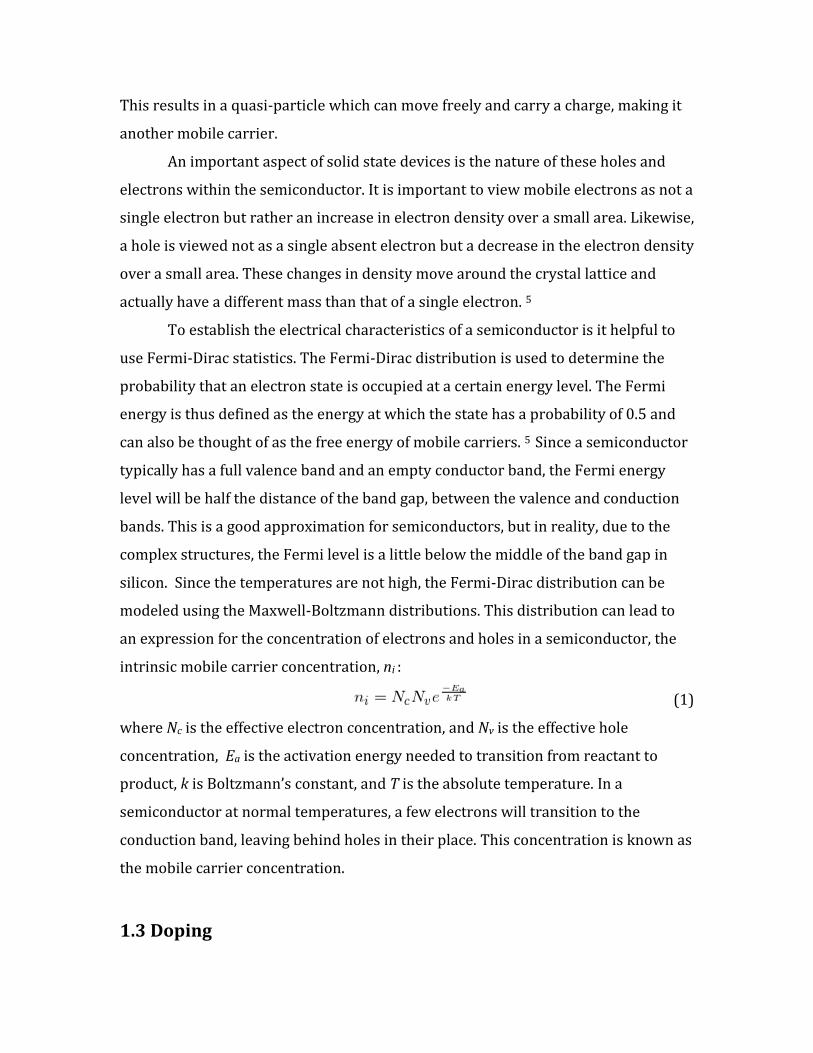
An important aspect of solid state devices is the nature of these holes and

electrons within the semiconductor. It is important to view mobile electrons as not a

single electron but rather an increase in electron density over a small area. Likewise,

a hole is viewed not as a single absent electron but a decrease in the electron density

over a small area. These changes in density move around the crystal lattice and

actually have a different mass than that of a single electron. 5

To establish the electrical characteristics of a semiconductor is it helpful to

use Fermi-Dirac statistics. The Fermi-Dirac distribution is used to determine the

probability that an electron state is occupied at a certain energy level. The Fermi

energy is thus defined as the energy at which the state has a probability of 0.5 and

can also be thought of as the free energy of mobile carriers. 5 Since a semiconductor

typically has a full valence band and an empty conductor band, the Fermi energy

level will be half the distance of the band gap, between the valence and conduction

bands. This is a good approximation for semiconductors, but in reality, due to the

complex structures, the Fermi level is a little below the middle of the band gap in

silicon. Since the temperatures are not high, the Fermi-Dirac distribution can be

modeled using the Maxwell-Boltzmann distributions. This distribution can lead to

an expression for the concentration of electrons and holes in a semiconductor, the

intrinsic mobile carrier concentration, ni :

(1)

where Nc is the effective electron concentration, and Nv is the effective hole

concentration, Ea is the activation energy needed to transition from reactant to

product, k is Boltzmann’s constant, and T is the absolute temperature. In a

semiconductor at normal temperatures, a few electrons will transition to the

conduction band, leaving behind holes in their place. This concentration is known as

the mobile carrier concentration.

1.3 Doping

The next critical aspect of semiconductor physics is doping. Doping occurs

with the insertion of shallow level impurities into a pure semiconductor. Supposed

an element such as phosphorous is added to a silicon crystal. Since phosphorus has

five free electrons, the first four will bond to the lattice with silicon, leaving one

extra electron unbonded. This extra electron occupies a donor state just below the

conduction band, but is excited up into the conduction band by the vibrational

energy of the lattice. 5 The electron then becomes delocalized, free to move about

the lattice. At this point, the phosphorus atom is considered a positively ionized

impurity. The result of this, is that by adding phosphorus to the silicon crystal, the

amount of conduction electrons has increased, thereby improving the overall

conductivity of the material.

The other method of doping introduces an element with three electrons

instead of five, such as boron. As a result, boron leaves an extra hole in just above

the valence band, called an acceptor state. The hole gets moved to the valence band

due to the vibrational energy of the crystal, and as a result creates a delocalized

negative mobile carrier. This makes boron a negatively ionized impurity. Similarly

to the phosphorus, by adding boron, the overall conductivity of the semiconductor

has increased.

Typically, Group VB elements such as phosphorus are considered donor

impurities, while Group IIIB elements act as acceptor impurities. These impurities

are called dopants. If the doping is done with a donor impurity, it is called n-type

doping because more electrons are being sent to the conduction band, making the

majority of the mobile carriers negatively charged. Conversely, if the doping is done

with donor impurities, it is called p-type doping because more holes are being sent

to the valence band, making the majority of the mobile carriers positively charged.

When doing p and n-type doping it is important to clarify the different types

of mobile carriers. First, there are intrinsic mobile carriers, the electrons and holes

that are free to move in a pure semiconductor crystal. Second, there are majority

carriers, which correspond to electrons in n-type and holes in p-type

semiconductors. Finally, there are minority carriers, which are holes in n-type and

electrons in p-type semiconductors. The majority carrier is usually orders of

magnitude larger than the minority and intrinsic carriers, although minority

carriers are a vital part of the inversion process. Having a large proportion of

majority carriers will cause a shift in the Fermi energy level. 5 It is self-evident, that

if there are more electrons in the conduction band that the energy level (Fermi

level) where there is a 50% chance of being occupied must shift towards the

conduction band. Similarly, the Fermi level will shift closer towards the valence

band when holes are the majority carrier. Typically, doping is done using ion

implantation.

1.4 Wafer Fabrication

In order to make an integrated circuit, the first step is to fabricate a wafer.

These wafers are composed of single crystal silicon. The silicon comes from sand

which contains SiO2. In order to get high grade silicon, the silicon dioxide must first

be reduced:

SiO2 + 2C → Si + 2CO

The silicon must then be purified again using hydrogen chloride:

Si + 3HCl → SiHCl3 + H2

The SiHCl3 is then distilled and reduced until only high grade polycrystalline

material is left over.

Once electronic grade silicon has been obtained, it is possible to grow a wafer.

The main technique for wafer growth is the Czochralski (CZ) process.6 In CZ growth,

the pure silicon is placed into a crucible and then heated until it melts. A crystal seed

is then placed into the molten silicon. Note that the diamond cubic structure of

silicon allows for multiple orientations which have different electrical properties.

Depending on the device being fabricated with the wafer, a different crystal with a

different orientation will be used as the seed. The seed is slowly pulled up until the

desired wafer size is solidified on the crystal. From there the crystal structure is

gradually pulled up until a larger crystal is formed. Once the large crystal is cooled it

is then cut into thin slices, making the silicon wafers7.

Another method used to make wafers is Float Zone (FZ) refining. In this

method, a silicon rod is melted and then recrystallized. The recrystallized rod then

goes through a furnace, which only heats one section (zone) at a time. The

impurities are thus moved to the bottom of the rod. The rod continues cycle through

the furnace until the desired purity has been reached. As a result, the FZ method

gives the purest silicon.8 However, the impurities found in the CZ process actually

improve the durability and reliability of the wafers by increasing the mechanical

strength and allowing for internal gettering which will be discussed shortly.

Therefore CZ growth is used primarily for industrial applications which don’t

require extremely pure silicon.

2.2 Impurities and Gettering

In any silicon wafer there will be some impurities that affect the properties of

the semiconductor. For instance, doping atoms can be thought of as point defects

within the crystal. Foreign atoms can contaminate the crystal by either forming in

the lattice or inside the lattice structure (interstitial).9 These atoms typically form

electronic states inside the band gap which cause poor electronic performance. In

addition, these atoms can group together to form precipitates within the crystal,

which will cause device failure.

While most foreign atoms have negative effects, not all do. One example is of

a beneficial foreign atom is oxygen. In the CZ process, oxygen is dissolved into the

crystal from the crucible, forming interstitial impurities. As long as the oxygen

amount is small enough to not form precipitates, it can provide two beneficial

characteristics. The first is to improve the mechanical durability of the crystal. The

second is to add donor states into the crystal, adding extra doping to the crystal.

During the CZ process, great care must be taken to not introduce carbon, which will

accelerate the formation of oxygen precipitates.9

Following the discussion of impurities, it is important to mention gettering.

Gettering is a process used to move impurities from active areas in the device. This

is crucial to ensure device reliability and durability. The underlying principle behind

gettering is that a damaged section of a crystal lattice will “get” or capture defects

and foreign impurities.10 Since there is already a defect, it takes less energy for

impurities to fall into the defect than to form an interstitial defect in the lattice. In

external gettering, the back is typically damaged so the front (where the ICs are

placed) will not have defects. The “damage” is usually caused by adding argon ions

or polysilicon to the back of the wafer which draw out the defects. Alternatively,

internal damages can be used to trap and collect defects which typically done with

oxygen atoms. The first step is to remove the oxygen from the front of the wafer by

heating it, causing the oxygen to move out of the surface. The wafer is then

annealed, allowing for the remaining oxygen atoms to cluster together, nucleating.

Once the nucleation reaches as critical mass it will then cause defects inside the

crystal which can be used for gettering. Internal gettering has become more popular

in the recent years due to its simplicity and use of existing elements in the

fabrication process.

2.3 Oxide Growth

Once a wafer has been fabricated, the next step is oxidation. An oxide layer

provides insulation for the semiconductor which is crucial for capacitors. The

primary advantage of silicon versus other semiconductors (germanium) is that it

easy combines to make silicon dioxide. By heating up the wafer in a container filled

with oxygen, a glass film (thermal oxide), is formed (thermal oxidation). Note that

quartz glass is an amorphous and not a solid crystal. Thermal oxidation is preferred

over chemical vapor deposition (CVD) because it provides a more uniformed

structure that is less subject to change over time.9 Another critical property of

amorphous silicon dioxide is that it provides a mask for doping, due to a low

diffusion rates.

There are two main methods of oxidation: dry oxidation and wet oxidation.

Dry oxidation occurs by heating the silicon wafer in a chamber filled with oxygen

gas. The result is silicon dioxide. Wet oxidation occurs by heating the silicon wafer

in a chamber filled with water vapor. The result is silicon dioxide and hydrogen gas.

It is crucial to closely monitor the temperature and amounts of each substance in

these reactions. In order to get the desired device specifications, exact thicknesses

and timings are required. The growth of the thin film and the time required can be

modeled using the Deal-Grove model11.

Under the Deal-Grove model, thermal oxidation is broken into transport and

reaction processes. The oxygen gas in the chamber moves first (transports) to the

silicon surface. Next the oxygen diffuses and dissolves (reaction) into the interface

of gas and solid. The Deal-Grove model then gives two useful expressions for the

oxide thickness and growth time.12 The first, called the parabolic growth regime, is

diffusion limited, meaning that the limiting factor is the diffusion of oxygen through

the oxide film. The second expression, the linear growth regime, is considered mass

transport limited, meaning that the limiting factor is not enough oxygen close to the

substrate. The parabolic regime expression is given by:

(2)

where x is the oxide layer thickness, B is the parabolic rate constant that can be

found in a lookup table, and t is the time. Similarly, the linear limiting expression is:

(3)

where B/A is the linear rate constant that can be found in a lookup table, t0 is the

initial time, x is the oxide thickness, and t is the time.

The growth of thin films is also highly correlated to temperature.12The linear

and parabolic growth rate constants can be related to temperature via the Arrhenius

equation:

(4)

Where R is the rate constant, R0 is the initial rate constant, Ea is the activation

energy needed to transition from reactant to product, k is Boltzmann’s constant, and

T is the absolute temperature. The activation is usually around 2 eVs whereas the

initial rate constants are ~ 104.

A final consideration in growth of thermal oxides is the pressure. Increasing

the pressure will cause more oxygen atoms to move to surface, decreasing the

overall time needed to reach a desired thickness. This is important in industrial

settings where it is necessary to limit the amount of high temperature the substrate

is exposed to, in order to mitigate negative effects on durability. Decreasing the

temperature will simultaneously increasing the pressure will allow the wafers to be

fabricated in the same amount of time. Another industrial application of pressure

dependence is the ability to make very thin films by using a lower pressure. In

summary, the Deal-Grove model is used in industrial settings to model the required

device parameters.

3.1 Material Interfaces

Before getting into the specifics of metal-oxide-semiconductor capacitors it is

important to analyze the properties at the interface of different materials. Recall

that Fermi energy is the free energy of mobile carriers which implies that at

equilibrium, the Fermi level of a solid will be uniform. In addition to the Fermi level,

the work function is used to describe the electronic properties at material interfaces.

The work function is defined as the energy required to remove an electron from a

material in a vacuum. It can be thought of as the energy difference between the

Fermi level and the vacuum, and as a result each material will have a different work

function. For a given work function, there is also an associated threshold voltage at

which current will begin flowing, activating the device. 13 This threshold voltage is

typically a few volts.

Now, with this knowledge, it is possible to analyze the interface of a metal

and a semiconductor. Since intrinsic (undoped) semiconductors have a larger work

function than metals, when the two materials are placed together, the electrons will

flow from the metal to the semiconductor until equilibrium is reached. The electrons

flow from the metal to the semiconductor because the semiconductor has a lower

Fermi level (lower energy states). Because electrons are being added to the

conduction band of the semiconductor, it is essentially being n doped close to the

interface, causing a shift in the Fermi level. Since the Fermi level must remain

constant, the bands must “bend” close to the interface. The electrostatic field that is

caused by the potential differences between the two materials keeps the “bend” in

the bands near the interface. 13

Introducing doping to a semiconductor has a similar effect. For example, in a

p-type semiconductor, there will be a larger work function, and as a result there will

be a steeper “bend” in the band since more electrons will need to travel from the

metal for equilibrium. Since p-type semiconductors have holes in the valence band,

these extra electrons will recombine with them first. This will cause a reduction in

the amount of mobile carriers available near the interface. If the semiconductor is

heavily doped (>1018 cm-3), holes will still remain the majority carrier, but will be

reduced. This is called depletion.14 If the doping level is low enough (<1013 cm-3), all

the holes will be recombined with electrons in the valence band, and the electrons

will then move to the valence band. This changes the majority carrier from holes to

electrons, making the p-type semiconductor n-type at the interface. This is called

inversion. 14

Similarly, if one has combines a metal to an n-type semiconductor, there will

also be a "bend" in the bands of the semiconductor near the interface. Electrons

travel from the metal to the semiconductor, entering the conduction band first as

there are no holes in the valence band. This will cause an increase in the amount n-

type dopants in the semiconductor. This process is called accumulation because the

amount of mobile carriers increases. 14 Also, it is possible to have the Fermi level

and the work function difference of the materials cancel out with the right doping

concentration. Since the effective work function difference is zero, there is no

"bend" in the band. This is called flat-band.14

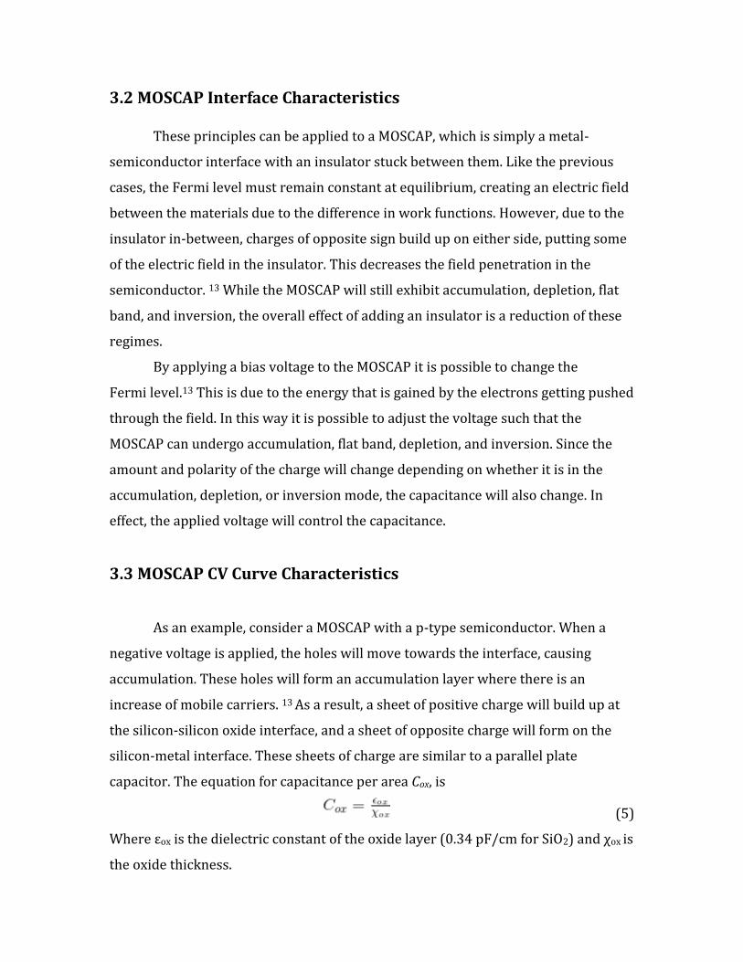
3.2 MOSCAP Interface Characteristics

These principles can be applied to a MOSCAP, which is simply a metal-

semiconductor interface with an insulator stuck between them. Like the previous

cases, the Fermi level must remain constant at equilibrium, creating an electric field

between the materials due to the difference in work functions. However, due to the

insulator in-between, charges of opposite sign build up on either side, putting some

of the electric field in the insulator. This decreases the field penetration in the

semiconductor. 13 While the MOSCAP will still exhibit accumulation, depletion, flat

band, and inversion, the overall effect of adding an insulator is a reduction of these

regimes.

By applying a bias voltage to the MOSCAP it is possible to change the

Fermi level.13 This is due to the energy that is gained by the electrons getting pushed

through the field. In this way it is possible to adjust the voltage such that the

MOSCAP can undergo accumulation, flat band, depletion, and inversion. Since the

amount and polarity of the charge will change depending on whether it is in the

accumulation, depletion, or inversion mode, the capacitance will also change. In

effect, the applied voltage will control the capacitance.

3.3 MOSCAP CV Curve Characteristics

As an example, consider a MOSCAP with a p-type semiconductor. When a

negative voltage is applied, the holes will move towards the interface, causing

accumulation. These holes will form an accumulation layer where there is an

increase of mobile carriers. 13 As a result, a sheet of positive charge will build up at

the silicon-silicon oxide interface, and a sheet of opposite charge will form on the

silicon-metal interface. These sheets of charge are similar to a parallel plate

capacitor. The equation for capacitance per area Cox, is

(5)

Where εox is the dielectric constant of the oxide layer (0.34 pF/cm for SiO2) and χox is

the oxide thickness.

As the voltage increases (positively), the amount of mobile carriers (holes)

will decrease until the flat band is reached. When the voltage increases, the

capacitor will enter into depletion. In this regime, the positive voltages will repel the

holes from the oxide interface. The region without the holes is called the depletion

region. 13 This region has an overall negative charge. As a result the capacitance can

again be modeled as a parallel plate capacitor with the depletion capacitance, Cd, per

area given by:

(6)

where εs is the semiconductor dielectric constant and χd is the depletion layer

width.

As the voltage gets very large, the MOSCAP will undergo inversion. In this

regime, the positive bias is such that the majority carriers (holes) are pushed away

from the interface and the minority carriers (electrons) are attracted to the

interface. The sheet of electrons form an inversion layer within the depletion layer,

halting the growth of the depletion layer. 13 The result is that the semiconductor

becomes n-type at the interface. The capacitance per area, Cs, is given by:

(7)

where χsmax is the maximum depletion layer width.

To measure the CV curve of a MOSCAP, the silicon-silicon oxide wafers are

coated with a metal (aluminum) or polysilicon (used for transistor fabrication). 15

To improve conductivity, the back of the silicon wafer may also be coated with a

metal. The two metal contacts are then connected to an impedance analyzer which

applies a voltage sweep, measures the current, and calculates the capacitance by

integrating the current over time. In a perfect MOSCAP there would be no current

inside the oxide insulator, however in real world systems there is typically a small

leakage current which is accounted for in most modern measurement systems. 16

The MOSCAP CV characteristics are illustrated by the following chart17:

Figure 1: CV Characteristics of MOSCAP

CV measurements are typically done at low (quasistatic) and high

frequencies. 5At low frequencies (Hz range), the mobile carriers will be at the oxide

interface during accumulation and inversion, making the MOSCAP capacitance equal

to the total capacitance of the oxide layer. In the depletion mode, since there are no

mobile carriers at the oxide interface, the total capacitance will be the series

combination of the depleted region and the non-depleted region, decreasing the

overall capacitance.5 In high frequency measurements (MHz range), the total

capacitance for the accumulation and depletion modes are the same as in the low

frequency range. However, in the inversion mode, the high frequency is too fast for

an inversion layer to form.5 As a result, the total capacitance for the inversion mode

is the same as for the depleted mode, the series combination of depletion and oxide

capacitance.

4.1 Oxide Charges

Now, the CV characteristics of MOSCAPs are further complicated by the

introduction of trapped charges in the oxide layer during fabrication. These charges

are effectively trapped inside the oxide layer, near the oxide interface, and therefore

affect the depletion region by shifting the potential.16 These charges are called oxide

charges and are divided into four types: interface trapped charges (also known as

surface states), fixed oxide charges, oxide trapped charges, and mobile oxide

charges. Surface states are caused by structural defects and are typically removed

using a low temperature annealing process. Oxide trapped charges are holes or

electrons that are trapped from ionizing radiation. These can also be removed using

low temperature annealing. Mobile oxide charges are contaminants from Na+, Li+, or

K+ ions that can occur during the fabrication process. These charges are often

identified using a bias stress test. Fixed oxide charges are typically positive charges

located near the semiconductor-oxide interface and are a result of the thermal

oxidation process. 16 These charges are the primary interest of this paper.

It is helpful to analyze the effect of the fixed oxide charges using the flat band

condition. The flat band capacitance, CFB, can be shown to be:

(8)

where Cmax and Cmin are the maximum and minimum capacitance, NA and ND are the

acceptor and donor concentrations, and ni is the intrinsic carrier concentration.

Once the flat band capacitance has been calculated, the flat band voltage can

be visually determined from the CV curve. If the charges are assumed to be stuck

near the interface, an expression for the flat band voltage, VFB, can be given as:

(9)

where φM and φS are the work functions for metal and semiconductor, and Qf is the

fixed charge density near the surface of the oxide. For a given MOSCAP, the change

in flat band voltages, called the flat band shift, can be found using:

(10)

Finally, in the inversion regime, it is possible to calculate the threshold voltage, VT, of

the MOSCAP. This equation is given by:

(11)

where φF is the work function of the Fermi energy level, and NB is the substrate

charge concentration. The important feature of this expression is that the change in

the threshold voltage will be the flat band shift for the same MOSCAP with different

trapped charge amounts.

So,

(12)

Since the threshold voltage is a critical parameter for MOS devices14,

(especially CMOS transistors), it will be possible to relate a change in fixed oxide

charges, Qf, with the overall performance of these devices using the above equations

and two MOSCAP CV curves (with and without oxide charges).

Methods

In order to test how the oxide charges affect device performance, capacitance

and voltage curves were taken. CV curves, as explained previously, show the

effective capacitance as a function of different voltage biases applied to the metal

contacts. By measuring the CV curve for a MOSCAP with trapped charges, and

comparing it to one without charges, it would be possible to see a change in

characteristic behavior of the capacitor, and therefore infer the change in

performance.

Originally, an experiment was planned using MOSCAPs manufactured at

SHARP Labs in Camas, Washington. These were made as P type silicon with boron

doping and oxide thickness of 110 nm, (see appendix). These wafers were then

broken into smaller pieces. The backsides of these pieces were scratched and light

layers of a conductive silver paste were added, in order to improve the metal

contacts. Once the silver had dried after about 3 days, the wafers were placed into a

measuring stage, where the wire leads were placed on the metal contacts using a

microscope. After the connection was made, a HP 4275A impedance analyzer was

used to measure the capacitance from -5 to +5 Volts using an alternating current of

1 MHz. These readings were then connected to ICS software on a computer.

Unfortunately, after repeated trials, there was no viable data measured just

static noise. After switching to a HP 4192A and then a Solartron SI 1260, no results

were measured. During the measurements with the Solartron, there was a failure,

likely a blown capacitor, which caused the Solartron to be under repair for a few

days. After trying again with the Solartron without results, a new strategy was

devised.

The measurements could be simulated using software tools developed for

MOSCAPs. The particular software used was based on PADRE. Two measurements

were taken using simulated MOSCAPs: one with trapped charges, and another

without trapped charges. In this way, the only variable changed was the amount of

charges introduced into the oxide layer. A trapped charge density of 1016 cm-3 was

added in order to provide an extreme difference between the two simulated

MOSCAPs. In the simulated MOSCAPs, the wafers were P doped, with an insulator

thickness of 0.1 micrometers. The measurements were simulated with a bias of -5 to

+5 Volts, with an alternating current of 5 MHz and 1 Hz.

Results and Discussion

The results of the simulations were then calculated using the PADRE18 and

MOSCap19 software and are shown in the following graph:

Figure 2: CV response of contaminated (blue/yellow) and uncontaminated (magenta/green) MOSCAPs.

On the graph, the blue line corresponds to the high frequency response and

the yellow line corresponds to the low frequency response of the MOSCAP with

trapped charges. Also, the magenta line corresponds to the high frequency response

and the green line corresponds to the low frequency response of the MOSCAP

without trapped charges. Note the accumulation regime at negative voltages,

depletion, flat band, and inversion at positive voltages.

As is visible from the graph, there is a noticeable shift in the CV curves of

approximately 1 Volt. This shift corresponds to a change in the flat band voltage

(equation 10). Since the threshold voltage is dependent on flat band voltage

(equation 12), there will also be a shift in threshold voltage. As noted earlier, the

threshold voltage is a critical parameter used in field-effect devices. Since the typical

threshold voltages are close to 0.7 mV, a shift of 1 Volt will cause a dramatic change

in the voltage needed to activate the device. This will have a negative effect on the

reliability of the devices because they will be operating outside the designed

tolerances. As a result, the trapped oxide charges will have a significant negative

impact on device performance.

Conclusion

During the fabrication of MOSCAPs contaminants can be trapped inside the

oxide layer. By introducing oxide charges into the MOSCAP the threshold voltage

shifts causing device instability and general reliability problems. As a result,

MOSCAP devices suffer worse performance with trapped charges than without

trapped charges. For large scale industrial applications, this can be catastrophic. It is

crucial for production that these trapped charges be kept to a density under 1015

cm-3. With modern clean room procedures and annealing processes it is standard to

have densities well below 1015 cm-3. Nonetheless, trapped charges can still cause

problems in device performance if they are not carefully tested for.

Recommendations

One recommendation is the need for physical measurements. Do to

equipment malfunctions and general technical issues; I was unable to use the

impedance analyzer with the fabricated wafers. It would be very beneficial to

compare those readings to those of the simulated results to determine the accuracy

of the measurements.

Another recommendation would be to study the effects of mobile charges

such as sodium or potassium ions. It would be possible to contaminate the MOSCAP

with a sodium or potassium bath, and measure the shift in the CV curve. This shift

could be used to calculate the shift in the flat band voltage, as well as determine the

mobility and diffusivity of the charges.

Acknowledgements

I would first like to acknowledge my advisor Dr. Solanki for the use of his

equipment and continued guidance with my project. I would also like to thank Dr.

Evans and Sharp Labs for fabricating the MOSCAPs and starting me on this project.

In addition, I would like to thank Prasanna Padigi for teaching me how to use the lab

equipment and for advising me on any questions I had. Finally, I would like to thank

Dr. Fallon, Dr. Wolf, Dr. Estes, and the Portland State University Urban Honors

College for their guidance and support of my undergraduate thesis.

Appendix A – Wafer Fabrication Data Sheet

Appendix A - Continued

References

1. Griffiths, David (1995). Introduction to Quantum Mechanics. Prentice Hall.

ISBN 0-13-124405-1.

2. Boeyens, J. C. A.: Chemistry from First Principles. Berlin: Springer Science

2008, ISBN 978-1-4020-8546-8

3. IUPAC. Compendium of Chemical Terminology, 2nd ed. (the "Gold Book").

Compiled by A. D. McNaught and A. Wilkinson. Blackwell Scientific

Publications, Oxford (1997).

4. Shyam P. Murarka and Martin C. Peckarar, Electronic Materials: Science and

Technology, Academic Press, Boston, 1989.

5. Andrew S. Grove, Physics and Technology of Semiconductor Devices, Wiley,

New York, 1967.

6. J. Czochralski (1918) "Ein neues Verfahren zur Messung der

Kristallisationsgeschwindigkeit der Metalle" [A new method for the

measurement of the crystallization rate of metals], Zeitschrift für

Physikalische Chemie, 92 : 219–221

7. Paweł Tomaszewski, "Jan Czochralski i jego metoda" (Jan Czochralski and his

method), Oficyna Wydawnicza ATUT, Wrocław–Kcynia 2003, ISBN 83-

89247-27-5

8. William G. Pfann (1966) Zone Melting, 2nd edition, John Wiley & Sons

9. Mattox, Donald M. (2010). Handbook of Physical Vapor Deposition (PVD)

Processing (2 ed.). ISBN 0815520387.

10. Rozgonyi, G. A., and C. W. Pearce. "Gettering of surface and bulk impurities in

Czochralski silicon wafers." Applied Physics Letters 32.11 (1978): 747-749.

11. Deal, B. E.; A. S. Grove (December 1965). "General Relationship for the

Thermal Oxidation of Silicon". Journal of Applied Physics 36

12. Jaeger, Richard C. (2002). "Thermal Oxidation of Silicon". Introduction to

Microelectronic Fabrication (2nd Ed.). Upper Saddle River: Prentice

Hall. ISBN 0-201-44494-1.

13. E. H. Nicollian and J. R. Brews, MOS Physics and Technology, Wiley, New York,

1982-2nd Ed. 2003.

14. S. M. Sze, Physics of Semiconductor Devices, Second Edition, New York: Wiley

and Sons, 1981.

15. Stephen A. Campbell, The Science and Engineering of Microelectronic

Fabrication, Oxford University Press, 1996-2nd Ed. 2001.

16. Schroder, Dieter K. Semiconductor material and device characterization. John

Wiley & Sons, 2006.

17. "Support." MOSCap Learning Materials. N.p., n.d. Web. 02 June 2015.

18. Mark R. Pinto; kent smith; Muhammad Alam; Steven Clark; Xufeng Wang;

Gerhard Klimeck; Dragica Vasileska (2014), "Padre,"

https://nanohub.org/resources/padre.

19. Akira Matsudaira; Saumitra Raj Mehrotra; Shaikh S. Ahmed; Gerhard

Klimeck; Dragica Vasileska (2014), "MOSCap,"

https://nanohub.org/resources/moscap.