Mortgage Lending Institutions in Scandinavia:

A study of risk for the period 2000-2013

Authors: Syed Anil Akbar

Duyen Ngoc La

Supervisor: Catherine Lions

Student

Umeå School of Business and Economics

Spring semester 2014

Degree project, 30 hp

Abstract

In the last 14 years there has been a major flux in the Scandinavian financial institutions

and real estate markets. The increase in size and openness, in both the markets and the

institutions allowed the sector to expand phenomenally, raising concerns about the

potential rise of risks. Concerns regarding the health and state of the Scandinavian real

estate and mortgage markets increased with the surge in residential housing prices

between 2000 and 2013. However, during this period popular sentiments and media

outcry was not met with sufficient academic inquiry into the subject.

Hence, we conducted this study trying to bridge the gap between popular concern and

academic inquiry by addressing the question: How are mortgage lending institutions

affected by the risk emanating from residential real estate markets in Scandinavia

between 2000 and 2013? In attempting to answer this question we developed a two-

tiered approach by addressing two questions: What is the effect of selected factors on

the delinquency rate of mortgagors in Scandinavia during the period 2000 to 2013? And

does the change in institutional business models and mortgage lending businesses affect

their distance to default? These questions give us an insight into the composition of the

mortgage market and the effects of the market upon the institutional distress; thereby

giving us a comprehensive understanding of the markets and institutions in line with our

primary research question.

We employed a deductive approach in line with our epistemological stance of

positivism and ontological belief of objectivism. Thereby, we formulated a quantitative

explanatory research employing the panel regression analysis tools in order to address

our central question.

The results of the research re-affirmed our earlier intuition as we discovered that interest

rates, unemployment, outstanding mortgages and mortgage growth were significant

predictors of the delinquency rates. Meanwhile risk weighted assets, mortgage revenue

and mortgage share of total assets were significant predictors of distance to default.

These findings highlighted that while individual delinquencies are affected by macro

and mortgage business changes, the distress in institutions is characterized by capital

adequacy and the flux in their mortgage businesses.

Hence, the results of our two-tiered analysis confirmed that mortgage lending

institutions have been affected by the risks emanating from the residential real estate

markets between 2000 and 2013 and this effect has been characterized by changing

models and rising influence of the real estate market in institutional portfolios.

Keywords:

Scandinavia, Real estate markets, Mortgage, Delinquency, Firm Default, Distance to

default, Credit Risk, Panel regression, Random Effects model, Fixed Effects model

Acknowledgement

In developing this research, we owe our gratitude to people who helped us within this

process. Among the individuals who helped us in this process we would first like to

thank our supervisor Catherine Lions, whose help and supervision were vital for the

completion of this study. Secondly, we would give our regards to Jorgen Hellstrom for

his help with the development of the statistical model and contribution towards our

empirical research. Thirdly, we would like to give our regards to the faculty and the

administration of Umea School of Business and Economics, whose dedicated teaching

helped us in developing our insights, all throughout our degree program, and which

provided us with the necessary utilities for conducting this research. Finally, we would

like to thank our respective friends and family for their support all throughout this

process.

Umeå, May 23rd

2014

Syed Anil Akbar Duyen Ngoc La

Table of Contents

CHAPTER 1: INTRODUCTION 1

1.1 PROBLEM BACKGROUND 1 1.2 RESEARCH QUESTION 4 1.3 PURPOSE 5 1.4 RESEARCH GAP 6 1.5 CONTRIBUTIONS & LIMITATIONS 6 1.6 DISPOSITION 7

CHAPTER 2: METHODOLOGY OF THE RESEARCH 8

2.1 CHOICE OF TOPIC & PRECONCEPTIONS 8 2.2 PERSPECTIVE 8 2.3 RESEARCH PHILOSOPHY 9 2.3.1 EPISTEMOLOGY 9 2.3.2 ONTOLOGY 10 2.4 RESEARCH APPROACH 10 2.5 RESEARCH DESIGN 11 2.6 RESEARCH STRATEGY 12 2.7 TIME HORIZON 13 2.8 RESEARCH METHOD 14 2.9 LITERATURE AND DATA SOURCES 14 2.10 SUMMARY OF METHODOLOGY OF OUR RESEARCH 15 2.11 ETHICAL, LEGAL AND SOCIAL CONSIDERATIONS 16

CHAPTER 3: THEORETICAL FRAMEWORK 18

3.1 REAL ESTATE MARKETS, REAL ESTATE BUBBLES AND MORTGAGE MARKETS 18 3.1.1 THE REAL ESTATE MARKETS 18 3.1.2 REAL ESTATE BUBBLES 19 3.1.3 MORTGAGE MARKETS 21 3.1.4 THE COUNTRIES’ INSIGHTS 22 3.2 FINANCIAL RISKS IN BANKS AND FINANCIAL INSTITUTIONS 25 3.2.1 OPERATIONAL RISK 25 3.2.2 LIQUIDITY RISK 25 3.2.3 MARKET RISK 26 3.2.4 CREDIT RISK 26 3.3 RISK MANAGEMENT AND MEASUREMENTS 27 3.3.1 AN OVERVIEW 27 3.3.2 RISK AGGREGATION 28 3.3.3 RISK DECOMPOSITION 28 3.4 METHODS FOR RISK MANAGEMENT AND MEASUREMENTS 28 3.4.1 EXPERT SYSTEMS AND SUBJECT ANALYSIS 29 3.4.2 ACCOUNTING BASED CREDIT SCORING SYSTEMS 31 3.4.3 RISK OF RUIN MODELS 32 3.4.4 OUR CHOSEN MEASURE: DISTANCE TO DEFAULT 33 3.4.5 FACTORS INFLUENCING BANK / INSTITUTIONAL DISTRESS 33 3.5 RESEARCH MODEL 35

CHAPTER 4: PRACTICAL METHOD 37

4.1 HYPOTHESES 37

4.1.1 DELINQUENCY RATE OF MORTGAGORS 37 4.1.2 DISTANCE TO DEFAULT OF BANKS 40 4.2 DATA COLLECTION 43 4.3 COMPUTATION OF DTD 44 4.4 PANEL DATA AND STATISTICAL TEST FOR THE ANALYSIS OF PANEL DATA 45 4.4.1 PANEL DATA 45 4.4.2 FIXED AND RANDOM EFFECTS MODELS 46 4.4.3 DIAGNOSTICS TESTS 47

CHAPTER 5: EMPIRICAL RESEARCH 49

5.1 DESCRIPTIVE STATISTICS AND SUMMARY STATISTICS 49 5.1.1 RESEARCH QUESTION 1 49 5.1.2 RESEARCH QUESTION 2 52 5.2 REGRESSIONS AND TESTS 56 5.2.1 REGRESSION 1: DELINQUENCY RATE OF MORTGAGORS 56 5.2.2 REGRESSION 2: BANK DISTRESS 59 5.3 SUMMARY OF HYPOTHESES TESTED IN THE TWO MODELS 63

CHAPTER 6: DATA ANALYSIS 64

6.1. RESEARCH QUESTION 1 64 6.1.1 INTERPRETATIONS OF INDIVIDUAL HYPOTHESES 64 6.1.2 CONCLUSION ON SUB QUESTION 1 66 6.2. RESEARCH QUESTION 2 67 6.2.1 INTERPRETATIONS OF INDIVIDUAL HYPOTHESES 67 6.2.2 CONCLUSION ON SUB QUESTION 2 69 6.3. CONCLUSIONS ON THE MAIN RESEARCH QUESTION 69

CHAPTER 7: CONCLUSION 71

7.1 THE CREDIBILITY OF RESEARCH FINDINGS 71 7.1.1 RELIABILITY 71 7.1.2 VALIDITY 71 7.1.3 GENERALIZABILITY 72 7.2 CONCLUSION 72 7.3 FURTHER RESEARCH 74

REFERENCE LIST 76

List of Tables

Table 1 Summary of Main Procedure of Research Approach _____________________________________________ 12 Table 2 Summary of Research Strategy ___________________________________________________________________ 13 Table 3 Summary of Factors influencing distress in previous studies ____________________________________ 35 Table 4 Banks and LMLIS covered in the study____________________________________________________________ 44 Table 5 Data and data sources used in the study _________________________________________________________ 44 Table 6 Descriptive Statistics of Swedish Delinquency Model Variables _________________________________ 50 Table 7 Descriptive Statistics of Norwegian Delinquency Model Variables ______________________________ 51 Table 8 Descriptive Statistics of Danish Delinquency Model Variables __________________________________ 52 Table 9 Summary of Panel Data set _______________________________________________________________________ 53 Table 10 Summary of Statistics of the Banks Variables ___________________________________________________ 54 Table 11 Panel Data ________________________________________________________________________________________ 56 Table 12 Wooldridge test for Regression 1 ________________________________________________________________ 57 Table 13 Heteroskedasticity for Regression 1 _____________________________________________________________ 57 Table 14 Hausman test for Regression 1 __________________________________________________________________ 58 Table 15 Breusch-Pagan test for Regression 1 ____________________________________________________________ 58 Table 16 Fixed Effect Model for Regression 1 _____________________________________________________________ 59 Table 17 Wooldridge Test for Regression 2 _______________________________________________________________ 60 Table 18 Wald Test for Regression 2 ______________________________________________________________________ 61 Table 19 Hausman Test for Regression 2 __________________________________________________________________ 61 Table 20 Breusch-Pagan LM Test for Regression 2 _______________________________________________________ 61 Table 21 Pesaran Test for Regression 2 ___________________________________________________________________ 62 Table 22 Random Effects Model for Regression 2 _________________________________________________________ 63 Table 23 Summary of Hypotheses Tested in the Two Models _____________________________________________ 64 Table 24 Alpha Estimation for Regression 1 ______________________________________________________________ 65 Table 25 Alpha Estimation for Regression 2 ______________________________________________________________ 68

List of Figures Figure 1. Nordic House Prices _______________________________________________________________________________ 2 Figure 2. Household Debt in relation to Disposable Income _______________________________________________ 3 Figure 3. Summary of Methodology of the Research ______________________________________________________ 15 Figure 4. Equity as an Option of Asset _____________________________________________________________________ 32 Figure 5. The Research Model ______________________________________________________________________________ 35 Figure 6. Panel Summary Statistic _________________________________________________________________________ 46 Figure 7. The Research Model with Significant Factors___________________________________________________ 63

Abbreviations

BIS: Bank of International Settlements

EBSCO: Elton Bryson Stephens Company

EMF: European Mortgage Federation

FMAC: Freddie Mac

FMAE: Fannie Mae

FSA: Financial Supervisory Authority

IMF: International Monetary Funds

OECD: Organisation for Economic, Co-operation and Development

1

CHAPTER 1: INTRODUCTION

In this chapter we provide the readers with an introduction to our research topic. The

chapter discusses the background of the problem that lead us to the research question

followed by the purpose of the research, the research gap, limitations and contributions.

1.1 Problem Background

The Financial crisis of 2008-09 still haunts economists, industry professionals and

academics alike, especially in the wake of a slow recovery and the later development of

the crisis in Europe. Although a whole host of reasons have been discussed regarding

the causes of the financial crisis, the eventual spark that lit up the flame came after the

bursting of the property bubble. This leads to defaults on the subprime loans which

spelled out disastrous implications for the mortgage backed security markets; hence on

the financial markets as a whole (Jickling, 2009, p. 3-7). In light of these events heavy

criticism has been aimed towards both private and government backed subprime lending,

relaxed credit policies for mortgages, and upon the failure of risk management within

corporate lending institutions (Jickling, 2009, p. 6-7).

Large deviations from fundamentals within real estate markets can, hence, spell

potentially disastrous systemic effects upon an economy and the entire financial system

as a whole (Anson, 2012). This effect is especially pronounced in highly developed

markets where bank portfolios have a large exposure towards real estate investments

and housing mortgages make up a large part of the bank balance sheets. However, the

fundamental problem with real estate stems from the complexity of the real estate

market as it eludes notions of semi-strong efficiency present within other asset markets

particularly since transactions are mostly private and no liquid trading facilities are

present (Anson, 2012, p.45). Furthermore the excess availability of financing, easy

availability of credit and openness has made the housing market bubble prone within the

recent years, especially in times when crises lead to a flow of liquidity to safer assets.

Given these complications within the real estate market, the advent of the European

debt crisis spelled out a surge in the capital into the safer markets, which were relatively

well performing (Colliers, 2013). However, this effect was especially pronounced in

Scandinavia, which has one of the most transparent real estate markets in the world

(Colliers, 2013). Hence, within the last few years housing prices in Scandinavia have

increased significantly attracting criticism from the IMF, and noted economists like

Nourel Robini and Nobel Prize laureate Robert Schiller (Magnusson, 2013).

2

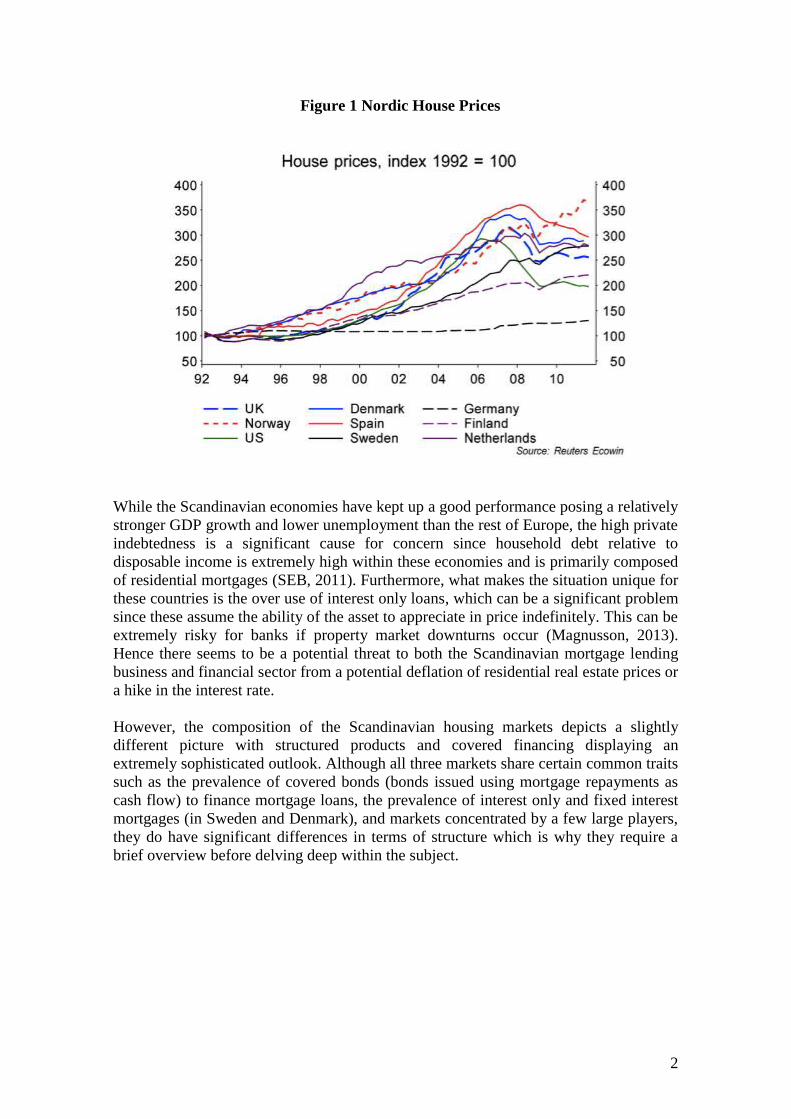
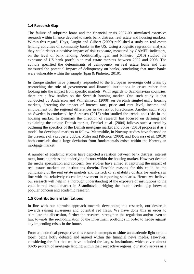
While the Scandinavian economies have kept up a good performance posing a relatively

stronger GDP growth and lower unemployment than the rest of Europe, the high private

indebtedness is a significant cause for concern since household debt relative to

disposable income is extremely high within these economies and is primarily composed

of residential mortgages (SEB, 2011). Furthermore, what makes the situation unique for

these countries is the over use of interest only loans, which can be a significant problem

since these assume the ability of the asset to appreciate in price indefinitely. This can be

extremely risky for banks if property market downturns occur (Magnusson, 2013).

Hence there seems to be a potential threat to both the Scandinavian mortgage lending

business and financial sector from a potential deflation of residential real estate prices or

a hike in the interest rate.

However, the composition of the Scandinavian housing markets depicts a slightly

different picture with structured products and covered financing displaying an

extremely sophisticated outlook. Although all three markets share certain common traits

such as the prevalence of covered bonds (bonds issued using mortgage repayments as

cash flow) to finance mortgage loans, the prevalence of interest only and fixed interest

mortgages (in Sweden and Denmark), and markets concentrated by a few large players,

they do have significant differences in terms of structure which is why they require a

brief overview before delving deep within the subject.

Figure 1 Nordic House Prices

3

The Swedish mortgage market is covered by eight large banks Danske Bank,

Handelsbanken, Lansforsakringar Bank, Nordea, SBAB Bank, SEB, Skandiabanken

and Swedbank, which control 95% of the market. Nordea, SEB, SwedBank and

Handelsbanken control assets 4.5 times the Swedish GDP and pose a strong Tier 1

capital ratio of 18% (Magnusson, 2013). In Sweden owner occupied and tenant owned

dwellings make up housing for two thirds of the population and loans pertaining to

housing make up almost 85% of household lending. Household debt has soared to 177%

of disposable income and housing prices have soared to 11% from 2009 (Magnusson,

2013). The Finans Inspektionen (Financial Service Authority in Sweden) has

implemented general guidelines to introduce a cap on the loan to value ratio at 85%.

However these make 11% of the total mortgage loans. This is pertaining to the fact that

the higher the loan to value ratio the more difficult it is to repay the loans. Sweden has

seen a growth in household indebtedness though lending institutions reiterate that they

have taken a stance by introducing limits to the indebtedness to 500% of the income.

The rate of amortization, however, stands at 140 years hinting signs of concern (FI,

2013).

Denmark, however, has a unique mortgage market, which even according to leading

investors such as George Soros (2008) offers a model for developed economies to

follow. Firstly only mortgage banks are allowed to offer loans against mortgages on real

property by issuing covered bonds on each mortgage. These banks are under strict rules

enforced by the Danish mortgage credit Act, which requires banks to match assets with

liabilities within their balance sheets. Only Five Large institutions: Nykredit, Realkredit

(part of the Danskebank group), Nordea Kredit (part of Nordea Group), BRF Kredit and

DLR Kredit control the entire mortgage market in Denmark. Secondly the government

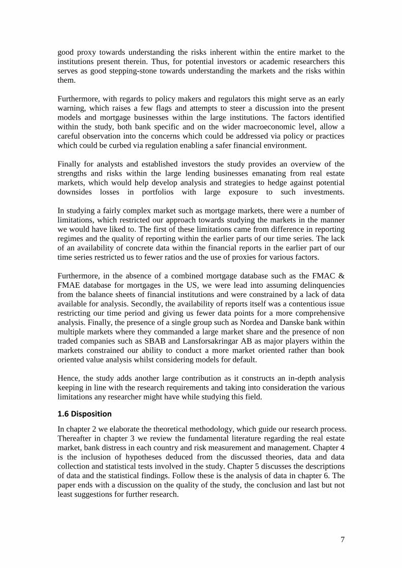
Figure 2 Household Debt in relation to Disposable Income

4

introduces a strict cap on loan to value ratios for different kinds of properties (BIS,

2004). However, the rise in unemployment and increase in household debt to 300% of

disposable income alongside the dampening of a property market bubble create

significant concern for the market and the financial sector as a whole (Lerving, 2014).

In comparison with those of its neighbours, Norway has a mortgage market in a

relatively nascent stage. The mortgage financing market is saturated by 3 large players

of whom DNB controls 35%, Sparebank 1 controls 13%, Nordea controls 11%, and 3

small players KLP, Storebrand and Terra which control less than 1% of the market

(regjeringen.no, 2012). Financing for mortgages is available mostly via adjustable rate

mortgages and mortgages of up to 70% of loan to value have to be covered by a covered

bond. Furthermore, banks provide plenty of cheap credit, which has increased

household debts considerably and household loans make up more than 85% of banks

assets. Government policy and subsidies encourage buying houses and the market has

seen a substantial increase during and after the credit crisis. Banks have increasingly

funded themselves using short term deposits from money markets which pose a

substantial problem since most of the balance sheet is composed of long term assets

(residential mortgages) (Gjedrem, 2010). However, Norwegian institutions have also

indulged in the distribution of controversial products such as securing credit lines on

houses and selling structured products with a derivative component, which have not

generated any substantial return for the investors and are potentially risky (Almklov,

2008).

Hence, despite the strengths of the structured and sophisticated Scandinavian mortgage

markets and financial institutions, there are some areas of legitimate concern, which

serve for an interesting case from a risk investigation perspective.

1.2 Research Question

Rapidly changing house prices, house price to income ratios, high levels of mortgage

debt as a share of household debt can be considered as signals towards housing bubbles.

A significant concern within such market conditions is the borrowers and institutions’

ability to indulge in speculation given the low interest rate conditions and in expectation

of ever increasing house prices (Boverket, 2013). In the event of a market downturn or

an interest rate hike this can spell disastrous consequences for financial institutions

involved in mortgage lending.

Furthermore, major financial institutions within Scandinavia have increasingly

expanded within the last 13 years, significantly changing their business model as well as

the risk appetite of their portfolios (FinansInspektionen, 2013, p.4). Hence, facing such

a situation we developed the following question, in line with our interest in mortgage

and real estate markets:

How are mortgage lending institutions affected by the risk emanating from the

residential real estate market in Scandinavia during the period 2000-2013?

In order to answer this question, we developed two sub-questions, which guide our

approach towards conducting this study. The two questions are:

What are the effects of selected factors on delinquency rate of mortgagors in

Scandinavia during the period 2000-2103?

5

Where the factors selected include indicators from established literature on the

predictors of delinquency. These include: mortgage interest rate, mortgage growth rate,

outstanding mortgage debt, debt to income ratio, unemployment rate, social benefits,

risk free rate, GDP growth rate and housing price changes.

Does the change in institutional business models and mortgage lending business affect

its distance to default?

Where the changing nature of business models and mortgage lending within institutions

is depicted by the following factors: mortgage growth, delinquency rates, derivatives as

a share of total assets, risk weighted assets, interbank assets, wholesale funding, net

income to total assets, loan to deposit ratio, mortgage revenue to total mortgage assets

and the share of mortgages within total assets.

1.3 Purpose

With increasing integration of financial markets and enlarging of the financial sector

within developed and developing economies, financial institutions have increasingly

acquired an important role within an economic system. Thus, the maintenance of

healthy financial markets and financial institutions is the objective of many

governments and has led international bodies like Bank for International Settlements,

OECD, IMF and World Bank develop regulation and procedures towards achieving this

objective. However, with regards to 2008 financial crisis and the later Euro debt crisis

concerns about the health of the financial system and institutions have been particularly

strong among investors, shareholders, governments and policy makers.

Hence, we attempt to address concerns about the health of major Scandinavian financial

institutions and their mortgage lending businesses in light of the tumultuous housing

markets via our study. Keeping investors, shareholders, analysts, policy makers and

advanced academic researchers as our target audience, we attempt to spread awareness

regarding risks posed from the changing bank business models and real estate markets

within Large Mortgage Lending Institutions (LMLIs) in the region.

In order to acquire a comprehensive overview of the evolution of the institutions, and to

account for a tumultuous period encompassing a rapid expansion followed by two crises

and an eventual slow recovery, we have chosen a period from 2000 to 2013 for our

study. The extent of this period will further the understanding of risks emanating from

the real estate markets, mortgage businesses and bank operations during volatile periods

and serve as a model encompassing stressed and expansive periods.

This study tries to develop a two-tiered approach towards the analysis of the primary

research question in order to serve as a useful insight for each of the members of the

intended audience. The first level involves the study into selected macro and micro

factors influencing delinquency. This would serve as an important insight into the

characteristics of the borrowers and the mortgage market itself, serving the needs of

policy makers, academics and industry analysts. The second level involves investigating

the factors affecting distress in large mortgage lending institutions within Scandinavia.

This would help display the risk emanating from business models and mortgage

businesses of the institutions, which draw them closer to distress thereby serving the

needs of investors, regulators and shareholders alike.

6

1.4 Research Gap

The failure of subprime loans and the financial crisis 2007-09 stimulated extensive

research within finance devoted towards bank distress, real estate and housing markets.

Within this regard, Hays, Lurgio and Gilbert (2009) published a study on real estate

lending activities of community banks in the US. Using a logistic regression analysis,

they could detect a positive impact of risk exposure, measured by CAMEL indicators,

on the level of bank lending. Additionally, Igan and Pinheiro (2010) studied the

exposure of US bank portfolio to real estate markets between 2002 and 2008. The

authors specified the determinants of delinquency on real estate loans and then

measured the potential impact of delinquency on banks, concluding that most banks

were vulnerable within the sample (Igan & Pinheiro, 2010).

In Europe studies have primarily responded to the European sovereign debt crisis by

researching the role of government and financial institutions in crises rather than

looking into the impact from specific markets. With regards to Scandinavian countries,

there are a few studies on the Swedish housing market. One such study is that

conducted by Andersson and Wilhelmsson (2008) on Swedish single-family housing

markets, detecting the impact of interest rate, price and rent level, income and

employment on the regional differences in the risk of foreclosure. Another such study

on Sweden is conducted by Sorensen (2013) who studied the trends and risks in the

housing market. In Denmark the direction of research has focused on defining and

explaining the unique Danish market, Frankel et al. (2004) follows such a trend by

outlining the specifics of the Danish mortgage market and Soros (2010) proposes it as a

model for developed markets to follow. Meanwhile, in Norway studies have focused on

the presence of a property bubble. Miles and Pillonca (2008), and Bourassa et al. (2010)

both conclude that a large deviation from fundamentals exists within the Norwegian

mortgage market.

A number of academic studies have depicted a relation between bank distress, interest

rates, housing prices and underlying factors within the housing market. However despite

the media speculation and concern, few studies have aimed at capturing the impact of

real estate markets on institutions therein. Possible reasons for this could be the

complexity of the real estate markets and the lack of availability of data for analysis in

line with the relatively recent improvement in reporting standards. Hence we believe

our research will help in a thorough understanding of the exposure of institutions to the

volatile real estate market in Scandinavia bridging the much needed gap between

popular concern and academic research.

1.5 Contributions & Limitations

In line with our alarmist approach towards developing this research, our desire is

towards raising awareness and potential red flags. We have done this in order to

stimulate the discussion, further the research, strengthen the regulation and/or even to

hint towards the re-modification of the investment portfolios in order to hedge against

any impending crises in the future.

From a theoretical perspective this research attempts to shine an academic light on the

topic, being hotly debated and argued within the financial news media. However,

considering the fact that we have included the largest institutions, which cover almost

80-95 percent of mortgage lending within their respective regions, our study serves as a

7

good proxy towards understanding the risks inherent within the entire market to the

institutions present therein. Thus, for potential investors or academic researchers this

serves as good stepping-stone towards understanding the markets and the risks within

them.

Furthermore, with regards to policy makers and regulators this might serve as an early

warning, which raises a few flags and attempts to steer a discussion into the present

models and mortgage businesses within the large institutions. The factors identified

within the study, both bank specific and on the wider macroeconomic level, allow a

careful observation into the concerns which could be addressed via policy or practices

which could be curbed via regulation enabling a safer financial environment.

Finally for analysts and established investors the study provides an overview of the

strengths and risks within the large lending businesses emanating from real estate

markets, which would help develop analysis and strategies to hedge against potential

downsides losses in portfolios with large exposure to such investments.

In studying a fairly complex market such as mortgage markets, there were a number of

limitations, which restricted our approach towards studying the markets in the manner

we would have liked to. The first of these limitations came from difference in reporting

regimes and the quality of reporting within the earlier parts of our time series. The lack

of an availability of concrete data within the financial reports in the earlier part of our

time series restricted us to fewer ratios and the use of proxies for various factors.

Furthermore, in the absence of a combined mortgage database such as the FMAC &

FMAE database for mortgages in the US, we were lead into assuming delinquencies

from the balance sheets of financial institutions and were constrained by a lack of data

available for analysis. Secondly, the availability of reports itself was a contentious issue

restricting our time period and giving us fewer data points for a more comprehensive

analysis. Finally, the presence of a single group such as Nordea and Danske bank within

multiple markets where they commanded a large market share and the presence of non

traded companies such as SBAB and Lansforsakringar AB as major players within the

markets constrained our ability to conduct a more market oriented rather than book

oriented value analysis whilst considering models for default.

Hence, the study adds another large contribution as it constructs an in-depth analysis

keeping in line with the research requirements and taking into consideration the various

limitations any researcher might have while studying this field.

1.6 Disposition

In chapter 2 we elaborate the theoretical methodology, which guide our research process.

Thereafter in chapter 3 we review the fundamental literature regarding the real estate

market, bank distress in each country and risk measurement and management. Chapter 4

is the inclusion of hypotheses deduced from the discussed theories, data and data

collection and statistical tests involved in the study. Chapter 5 discusses the descriptions

of data and the statistical findings. Follow these is the analysis of data in chapter 6. The

paper ends with a discussion on the quality of the study, the conclusion and last but not

least suggestions for further research.

8

CHAPTER 2: METHODOLOGY OF THE RESEARCH

This chapter entails theoretical considerations, which guide our research process. The

chapter starts with the choice, preconception of the research topic and the perspectives

the authors had in mind while conducting the research. The chapter also specifies the

philosophical underpinnings guiding the research and leads to the structure of the

research. Finally the chapter ends with a clarification of literature review, data sources

and the ethical, legal and social aspects of the thesis.

2.1 Choice of Topic & Preconceptions

The proposal of this research topic can be viewed as a combination of our knowledge

and interest within the subject. After gaining enough knowledge in Business

Administration and especially in finance, risk management and financial statistics, we

chose to conduct a study in line with our interests and relevant to the current affairs in

Scandinavia. Studying as foreign students in Sweden, we both were interested in

reconciling our concepts by studying a local issue and shining a light upon it from a

neutral’s perspective. Additionally, this research comes just in time when Scandinavia is

in a possible residential real estate bubble yet there is not enough corresponding

academic research within addressing this situation. Hence, we are very excited with the

prospects of our outcomes to fill the possible gaps within research.

However, our motivation for conducting research within this subject area should not be

assumed to generate subjectivity and influence our results. This stems primarily from

our training and education within both finance and research. As students who have had

the pleasure of studying and researching within different prestigious universities in

Europe, we believe we have acquired a necessary insight into both the subject matter of

finance and risk management, and a rigorous training in research projects which would

help us maintain objectivity within our research area. Furthermore, our different

backgrounds, analytical skills would increase the objectivity of the study process.

Moreover, we base our hypothesis on peered review theories/ models. The data is

established as it is represented in public domains, and statistical testing is in line with

credible input data. Finally, important critique and advice from our supervisor and

colleagues has increased the neutralist approach towards the research thereby enhancing

the validity of the thesis.

2.2 Perspective

Adhering to the purpose of our study, we will write our thesis in the perspective of

financial analysts attempting to understand the exposure of the real estate and mortgage

markets upon the financial market in Scandinavia. Our findings aim towards benefiting

a number of actors, namely banks, specialised investors, regulators, industry analysts

and advanced students of finance, the intended audience for this study. Therefore the

research employs specialised terminology and advanced financial concepts. Given the

soaring prices within the housing market, we expect our findings will reveal how

LMLIs have been affected by residential real estate market in Scandinavia. Thereby

helping investors hedge their risks, institutions gain an insight into and regulators to

plan appropriate policy responses for risks stemming from this market.

9

2.3 Research Philosophy

Research philosophy determines what reality is. Its importance is not only for the

development of knowledge but also for the nature of that knowledge (Saunders et al.,

2009, p. 107,108). The choice of one’s research philosophy helps one to define a good

research proposal and acquire useful guidelines throughout the course of research.

Epistemology and Ontology are the major orientations.

2.3.1 Epistemology

The epistemological stance concerns how to study a social entity. It asks whether a

social entity should be explained by ‘the same principles, procedures and ethos as

natural science’ or should it reflect the complexity of human behaviour and its

institutions (Bryman & Bell, 2011, p. 15, 16). Positivism and Interpretivism are the two

aspects of epistemology.

Positivism according to Crossman affirms the importance of imitating the natural

science given the use of appropriate methods (2003, p.50). Natural science implies

working with an observable social reality, which in turn leads to the production of

measurable data while appropriate methods refer to the use of ‘maths and formal logic’

to provide analytical statements about the observe world using the process of deduction

as the means of establishing generalisations and laws (2003, p.50). Carrying the features

of natural science, a positivist approach asserted by Saunders et al. (2009, p. 114)

should be undertaken in a value-free way which has to be assured by no bias

preferences of researchers in the collection of data and there should leave no room for

altering them. As Bryman and Bell (2011, p. 15) stresses that the true domain of a

positivist researcher should be scientific statements instead of normative statements.

Interpretivism opposes positivism, as it requires researchers to understand the

differences between objects and humans the latter of whom are social actors (Bryman &

Bell, 2011, p. 18; Saunders et al., 2009, p.116). According to this philosophical stance,

social science would become too rigid and limited if it only relied upon on hard facts

and observable reality since reality is not always observable or verifiable but multiple

and subjective. Crossman (2003, p.51, 52) stresses that reality is the creation of the

individual involved in the research and that humans are not objects but are subjects with

feelings, perceptions, behaviours and attitudes. Therefore, Saunders et al. agrees that

conducting research upon people is different from doing research on objects (2009, p.

115). Hence, the interpretive philosophy should adopt an empathetic stance, which

challenges researchers to enter the social world of the research subjects in order to

understand their point of views (2009, p. 116). Due to this feature Saunders et al. (2009,

p. 116) claims the interpretive perspective is more appropriate for studies on

organisational behaviour, marketing and human resource management.

A comparison of these features leads us to the conclusion that our study stands for

positivism. Adopting this view, we aimed to explain a reality in which possible causal

effects between social actors exist. We did not try to interpret human behaviour nor did

we try to understand in-depth phenomena beyond the observed reality since we believe

that knowledge is accepted only when it is logical and empirically verified (McKeinzie,

2011, p.535). Our research question “How are mortgage lending institutions affected by

the risk emanating from the residential real estate market in Scandinavia during the

period 2000-2013?” reflects this standpoint. First of all, there are no value judgements

in this question regarding the risk arising from the residential real estate market. The

10

question simply affirms the fact that mortgage lending institutions are exposed to

residential real estate market and initiates an inquiry into this affect. Then, acting like

natural scientists we believe knowledge originates from what we observe. In other

words, we based our research on observable social reality, namely LMLIs, banks as

institutions, mortgagors as individuals and the real estate market in Scandinavia from

where measurable data are collected. Lastly, following a deductive process we draw our

conclusions about the exposure of these institutions from the outcomes of the input data

and statistical tests leaving no rooms for subjective judgments as explained in the

interpretive position.

2.3.2 Ontology

The ontological stance deals with the nature of social entity – whether a social entity

exists independent of social actors or are social actors ones who build up social entities

(Saunders et al., 2009, p. 111). Responding to this question there are two orientations

objectivism and constructionism.

Objectivism implies that social phenomena confront us as external facts, which are

beyond our reach or influence (Bryman & Bell, 2011, p. 21). For the purpose of

convenience, both Bryman and Bell (2011, p. 21) and Saunders et al. (2009, p. 110,111)

develop the concept under an organisational set up. Every organisation has its own well-

defined structures, rules and missions. People living within this organisation simply

have to comply and fulfil their duties without any individual inputs upon how they are

to perform their jobs. In other words, the social entity is a constraining force of social

actors (Bryman & Bell, 2011, p.21).

On the other hand, a constructionist position asserts that ‘social phenomena and its

meaning is created from the perceptions and consequent actions of social actors’ (2009,

p. 21). Therefore, the researcher role is to try to understand the motives, actions and

intentions of social actors (Saunders et al., 2009). This goes in line with the

interpretivist philosophy, which stresses the importance of understanding the

complexity of human.

In this study a volatile real estate market is considered as a large organisation with

LMLIs, banks and mortgagors as individuals in this market. This organisation most

likely has a large impact on the individual participants in this set-up. The volatile

market condition within the period 2000-2013, there are potential issues which create

problems for mortgagors which consequently spread onto LMLIs. This impact is the

consequence of a causal effect. Delinquency rate and other market factors such as

housing prices and interest rate can be seen as mechanisms of the market, which

objectively affect mortgagors and LMLIs. Overall mortgagors and institutions bear all

possible impact from the real estate market, which will be revealed later in our analysis.

Hence for these reasons, we stand for the objectivist ontological position.

2.4 Research Approach

Having clarified our philosophical stance we can analyze our research approach in

conducting this study. This determines the relation of theory with our research and leads

to our research design (Bryman & Bell, 2011, p.11). The main consideration here is

testing and building theory. The two contrasting approaches are induction and deduction.

These have been illustrated in the following table.

11

The deductive approach is akin to scientific research, common in natural science

experiments (Collis & Hussey, 2003). Researchers adopt this approach by deducing a

hypothesis from a theory, indicating how data are collected, testing the hypothesis given

a certain strategy and confirming or modifying the theory in light of the findings

(Robson 2002; Bryman & Bell, 2011, p. 11).

However, the criticism of the deductive approach is that it is rigid and therefore limits

alternative explanations (Saunders et al., 2009, p.126). Therefore an alternative choice

is offered by the inductive approach. Within the inductive approach the research process

begins with data collection and concludes by drawing generalizations in the form of

inferences from the data creating a tentative hypotheses upon which conclusions are

drawn (Adams et al., 2007, p.29; Cresswell, 2009, p.63).

The difference of the two approaches can be observed from not only the research

process but also from the choice of data and research strategies, a discussion we will

conduct in the next section. However, before we continue, it is useful to associate the

different research philosophies with the research approaches. Deduction likely belongs

to positivism and induction to interpretivism (Saunders et al., 2009, p. 124; Bryman &

Bell, 2011, p.27).

In line with the philosophical stances clarified before and the sequence of the research

described above, our study adopted a deductive approach. As mentioned in the previous

part, with the understanding of fundamental theories, we can create hypotheses on the

predicted relationship of the delinquency rate and selected factors. We can also create

hypotheses on the impact of market factors and banks’ lending businesses on bank

distress. Thereafter collecting quantitative data and conducting subtle statistical tests,

we can confirm or reject the hypotheses to reinforce or negate the validity of the

theories. Therefore adhering to scientific method, we answer our research question

based on the outcome of the test built on initial theories.

2.5 Research Design

Research design is considered to be a general plan for the research (Saunders et al.,

2009, p. 136). In order to achieve a good plan, researchers need to be clear about the

purpose of their research since this will guide how the research is designed (Bryman &

Bell, 2011, p.40). According to Saunders et al. (2009, p.138) the purpose of a research

can be exploratory, descriptive and explanatory.

An exploratory study usually involves the exploration of new ideas, new insights or a

clarification of an ambiguous concept (2009, p. 139). This can be achieved by searching

literature, or conducting in-depth interviews such as those with an expert in field of

Source: Bryman and Bell (2012)

Table 1 Summary of Main Procedure of Research Approach

12

study or a focus group (2009, p. 139; Sreejesh et al. 2014, p.29, 30). Explanatory studies

according to Saunders et al. (2009, p.140) establish causal relationships between

variables. Researchers need to have good knowledge of the situation or phenomena in

order to infer or detect pertinent causal relationship (Zikmund et al., 2012, p.55).

According to Zikmund et al. (2012, p.55) researchers want to study how a change in one

event will change another event of interest.

In contrast with exploratory studies, design descriptive research emphasises upon the

description of a group of people or entities (Robson, 2002, p.59; Sreejesh et al., 2014, p.

33). Design descriptive research is further described by Sreejesh et al. (2014, p.33) who

discusses that it should describe the characteristics of certain groups in order to figure

out certain behaviour, to make specific prediction and to examine difference between

groups.

Hence based on the discussion above we can establish that our research design is

explanatory, since we emphasize on the relationship of the variables and seek to detect a

causal effect between them. We therefore believe that a possible causal relationship

between delinquency rate and other explanatory variables, such as disposable income,

employment, unemployment benefit, housing price etc exists. Furthermore, we also

believe the causal relationship between bank distress and the bank business model will

be examined in line with the objectives of an exploratory study.

2.6 Research Strategy

Having established the design of our research we progress towards our strategy. The

literature outlines numerous approaches towards conducting exploratory studies (Hair et

al., 2007; Robson, 2002; Saunders et al., 2009). Our choice however was in line with

our research philosophy and best suited towards addressing our research question

(Saunders et al., 2009, p. 141). The different strategies commonly used in social

sciences are:

When observing our research needs and philosophy alongside our questions, a research

strategy based on experimentation could not be implemented for the obvious lack of

control we possess on the independent variables. Archival data that we employed within

Source: Saunders et al., 2012, p. 171-188

Table 2 Summary of Research Strategy

13

our study cannot be changed within the context of the study; hence, our research cannot

be described as experimentation borrowing from a natural science context. The

principle for such studies as described in Bryman and Bell is establishing a control

group and an experimentation group upon whom individual tests are conducted by

changing the independent variables and observing the influence on the dependent

variables (2012, p.45). However, we have included a certain aspect of experimentation

within our study as we will be conducting an individual stress test upon the individual

institutions by changing the independent variables to assess the impact of a potential

impact of an unexpected negative stress event.

The study relies on secondary sources of information that are derived from established

reports and proxy variables constructed from established research, hence, surveys,

ethnographies, action research, case study, grounded theory or narrative inquiries can all

be ruled out as possible descriptions of our research. This is as all these are methods,

which rely on feedback from the research subjects and are the wider part of the

inductive approach towards research, which we have not pursued due to either the

complications involved within the collection procedures, the insufficient time and

resources to do so.

Hence, archival research as described before is the best description of the orientation of

our research strategy. This is as archival research described by Saunders is ‘research

that uses administrative data from the principle sources of data’ (Saunders et al., 2009, p.

150). Archival research is also described as one that makes use of data from the

principle sources and interprets it in order to derive conclusions not established before

by Hakim (1987, p.38-39). Since we employ data from secondary sources which has

been collected and organized this can reflect the reality embedded within statistics being

studied rather than being a poor reflection of data that might have been collected within

a different manner (Hakim et al., 1987, p. 21-24). Such an approach is best suited

towards answering our research question within the time frame in the most efficient

manner, as it uses established facts in the form statistical data to base conclusions upon.

We construct our macro-economic function of delinquency and default based on macro-

economic variables collected from the statistical bureaus of Sweden, Denmark and

Norway, while the model for distance to default is based on information from company

annual reports. This data has been used to derive our conclusions regarding our

hypothesis.

2.7 Time Horizon

Time horizons vary depending upon the purpose of a research question. If a researcher

is interested in a snapshot of a particular event at one given point in time, he/she fares a

cross-sectional study (Saunders et al., 2009, p.155). The purpose of this type of study is

to identify and understand differences between the various members of the study

population (Renmenyi et al., 1998, p.47). On the other hand, if the development or

changes of certain events are in concern, a longitudinal study is an alternative choice

(2009, p. 155).

Within our research, we are concerned with both types of studies. The reason is that we

are interested in both the differences between the exposure of mortgagors and LMLIs in

Sweden, Norway and Denmark and the credit risk evolving during the period of 2000-

2013. By just observing a snapshot of the credit conditions of the three countries at one

given time, we would be able to compare the differences in the rate of delinquency and

14

the impact of the mortgage lending business on bank distress in each country, but we

would not be able to see the development of particular variables for example the interest

rates or the credit risk throughout the economic cycle. By accounting for periods when

the economy was relatively healthy, onto a crash and into a recession our study

contributes a more in-depth understanding of delinquency and bank distress face from

credit risk ensuing from the real estate market.

2.8 Research Method

Research method provides us the framework of the data collection and data analysis. A

research can follow two widespread approaches - quantitative or qualitative approach.

The choice depends primarily on the purpose of the research question, whether the

emphasis is on generalisation or in-depth understanding (Bryman & Bell, 2011, p. 410).

Thereby, quantitative or qualitative data and deductive or inductive approach will be

matched respectively. Certainly these decisions need to follow after the choice of

researchers’ philosophical point of view.

According to a number of researchers there are common contrasts between the two

methods, which help them to determine the appropriate method. For instance,

qualitative research relies on contextual understanding of humans as social actors. This

requires the collection of qualitative data, which is rich and complex in meaning and

therefore requires the analysis of the words collected. In line with these characteristics,

theory and concepts in qualitative research emerge from data, which make the study

unstructured since it leaves room for subjective interpretations. On the other hand,

quantitative studies rely on generalisation, which needs the support of hard and reliable

data. This goes in line with the purpose of theoretical testing which follows a certain

static, pre-determined structure prescribed by researchers. Therefore quantitative studies

reflect a researchers’ point of view better than the views of participants in the research.

In this study we follow a quantitative method, which harmonises the purpose of our

research question and the choice of research philosophy, research approach and design.

This is as firstly the aim is to determine factors that lead to the delinquency by

mortgagors; for this we employ macro and micro factors in each country. The second

aim is to acquire the determinants of bank distress; for this we employ a number of

accounting ratios and fundamental theories on credit risk and risk management. The

statistics is collected from LMLI balance sheets, the statistical authorities in each

country and allow us to generate hypotheses that can be tested by statistical

programming software. Lastly, the confirmation or rejection of the stated hypotheses is

based on present theory and can only be made in the light of the outcomes without our

own interpretation.

2.9 Literature and Data Sources

In an attempt to ‘refine and map the already established theoretical framework’

(Tranfield et al., 2003, p.208) we utilized the literature and data from secondary sources.

Since this was in line with our deductive approach, literature review for which is done

for the purposes of establishing the theoretical framework for testing data (Saunders et

al., 2012, p.61). Secondary source analysis for the purposes of research is defined as the

analysis of sources, which have not been collected by the researchers themselves but

come from data collected by other researcher or by other organizations in the course of

their business (Bryman & Bell, 2011, p.325). This secondary data we have collected is

15

composed of data from reports, annual/quarterly statistics, scientific articles and books.

The literature primarily consists of material collected from Emerald and Business

Source Premier (EBSCO) and Science Direct available from Umea University library

and Reports from the individual financial authorities and central banks in the three

countries (Sweden, Norway and Denmark). The use of EBSCO and Science Direct

databases is a natural result of the fact that they consist of the largest source of

economics and business scholarly journals. The key words employed while conducting

our search were: residential real estate, credit risk exposure, banks, delinquency, default,

and distance to default, bank stress, Scandinavia, Sweden, Norway, Denmark, single

family house, mortgages, mortgage market, financial performance and risk report. In

gathering the literature we ensured that the articles were peer reviewed. This process

ensures the objectivity of the research.

After reviewing a sufficient number of articles and establishing a sound basis for our

research, we started gathering data for our models on defaults and distance to default

from Thomson DataStream, annual reports of individual banks and macro, micro

economic data from the European Mortgage Federation (EMF), OECD and Eurostat.

The choice of EMF, OECD and Eurostat database stem from their wide scope of

compiled data of different countries and in particular the specialised data on housing

and mortgage market from the EMF fit perfectly our research question. The choice of

Thomson DataStream stems from the acceptance and respect within the financial

community, it is regarded as a premier data source for businesses, academics and

industry analysts alike. Overall these databases underscore our utilization of globally

accepted, legitimate and verifiable data sources, which spells out the possibility of

incorrect data. However, in order to develop our model we had to create a new database

with micro and marco-economic variables alongside the financial statistics we collected.

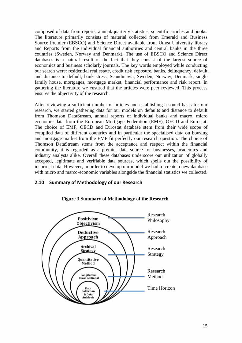
2.10 Summary of Methodology of our Research

Research

Philosophy

Research

Approach

Research

Strategy

Research

Method

Time Horizon

Figure 3 Summary of Methodology of the Research

16

2.11 Ethical, Legal and Social Considerations

Social science research is guided by ethical and legal considerations in order to ensure a

fair and justified approach towards research. A number of different schools argue the

different basis upon which to judge ethical and legal considerations within social

research. Two of the most prominent of these are universalism which argues that certain

universal ethics should not be broken by researchers in going about their research and

situation ethics which argue that ethics are defined by the situation faced by researchers

(Bryman & Bell, 2011, p.129). Since our research consists of a deductive approach with

descriptive/archival research we can associate with the universalism school of by

ensuring we have respected the specified ‘universal’ ethics and legal considerations of

research.

In discussing research ethics Diener & Crandall specify four specific parts of research

ethics. These concern the following whether there is harm to participants, whether there

is an invasion of privacy, whether there is a lack of informed consent and whether

deception is involved (1978, p. 17-96). In our research we employed data from

secondary sources where no individual participants were involved and large

organizations had disclosed information themselves, hence harm due to invasion of

privacy, lack of informed consent and harm to participants could not have been

involved in the data collection process as it was already a matter of public record

without any discrepancy and with full authority. Diener & Crandell elaborate on this

issue by mentioning that the fact that the disclosed information is a matter of public

records represents ‘informed consent’ by the companies involved (1978, p.38-39).

We addressed the concern regarding deception, which is explained as the ‘deliberate

misrepresentation of a scientific study’ (Diener & Crandell, 1978, p.72) by ensuring that

the sources were cited in the right context as per our understanding and it is correctly

cited with the corresponding author. However, deception also includes the process of

data processing and gathering. While conducting the econometric analysis, we have

ensured that this process is thoroughly elucidated with transparency. Furthermore, we

ensured a strict adherence towards presenting results as they occurred and have not

indulged in data mining in order to produce results. This can also be understood from

the fact that we have no gain in doing so nor do we have any established preconceptions

regarding the outcomes of our research.

Questions of ethical behaviour aside, we have also considered the legal aspects which

might afflict a research of this nature. The first of these refers to deception or

misrepresentation which we dealt with in the paragraph above by explaining the fact

that we have reproduced our research model, statistics and results with transparency in

the incoming chapters hence spelling out possibility of ‘data-mining’ or

misrepresentation of data. The second aspect concerns the issue of privacy and rights to

information. This aspect is covered by the fact that we have employed Thomson Reuters

DataStream and statistics from the Central Statistics Bureaus of Scandinavian countries.

Hence, all information used within this research is disclosed publicly and can be used

by anyone and does not create any privacy issues. We have, therefore, adhered to the

strictest provisions of ethics and legality while conducting this study.

In line with the legal and ethical aspects, we would also consider social or societal

impact of our research. Throughout our university studies we have constantly focused

on societal impact within our subject areas in order to become concerned and active

17

citizens within the wider community and in accordance with this spirit we continue this

trend within this research as well.

Adhering to the recent catastrophic events in the financial sector on the back of a

property market crash which left millions in financial turmoil particularly due to the

large exposure of the financial sector, we believe our study is a small attempt towards a

greater transparency and understanding of the risks facing the financial sector within

Scandinavia. We, via our study, have attempted to give a fair representation of the

exposure and consequent stress that could occur in a negative tail event. However, we

should elucidate that the purpose of our study is not to predict turmoil or to give reasons

for which would occur but merely understand what financial turmoil, if it occurs, could

do. This we believe is an extremely vital for not just investors, finance students and

institutions but ultimately also to the larger community involved in buying property and

taking mortgages. Thus adhering to our belief in greater transparency for the financial

services we believe our research has a potential to provide insights to buyers (via

mortgages) or their advisors and result in more awareness and understanding of risks

before the proverbial ‘rainy day’ occurs. Hence, essentially the societal impact of our

study is an attempt to increase the awareness and understanding of risks stemming from

the mortgage markets, which constitute a fairly large percentage of the credit markets

within Scandinavia.

18

CHAPTER 3: THEORETICAL FRAMEWORK

In this chapter we provide the theoretical framework on real estate and mortgage

markets. We then present the debate on real estate bubbles before going over the market

outlook for each Scandinavian country individually. Next we present the theoretical

underpinnings for the various concepts of financial risk and discuss the different

methods of risk measurements and risk management. The chapter ends by presenting

our selected measures and an illustration of our research model.

3.1 Real Estate Markets, Real Estate Bubbles and Mortgage Markets

3.1.1 The Real Estate Markets

In the recent financial history of the world few asset classes have created as much

controversy because of their potential role in financial crises as real estate. Despite

receiving a significant attention by academics and industry specialists alike, the

property or the real estate market remains a rather grey area, with researchers still

struggling to explain bubbles and mispricing within the market. A part of this problem

as argued by Anson (2012) lies in the fact that the real estate asset is fundamentally

illiquid in nature. This stems from a number of different factors such as the unique

nature of each property, the lack of a publicly traded market, appraisal valuing of each

asset and the ‘chunky’ size of this asset (Anson, 2012, p.45). The problem hence is that

there is no notion of efficiency within real estate markets where the price would

essentially reflect all publicly available information. Therefore essentially the problem

with real estate stems from the unique nature of the asset. Hence, in order to understand

real estate and consequently the mortgage market we will attempt to break down the

analysis to the very basics, by understanding the determinants of the real estate pricing

leading on to a discussion on the presence of large deviations or bubbles within the

market, before going over the analysis of the individual markets within the three

countries.

A great deal of research has gone into understanding the determinants of the cycles in

real estate prices from both the demand and supply side. Tsatsaronis and Zhu (2004) try

to summarize the main findings of prior research by explaining both the determinants

from the demand and supply side, including factors, which entail distortions within the

market. According to their research factors stemming from the demand side include

fundamentals such as nominal interest rate on bank loans (+), tax rate of first ownership

of house (+), cost of detention related amortization and maintenance (+) and earnings

and capital losses on housing (-). All of these factors are combined within one main

determinant, the user cost of housing which along with factors such as population size,

growth, disposable incomes (real/nominal) is used in composing the demand function.

Tsatsaronis and Zhu (2004) elaborate that factors, which determine supply are

availability of land, existence of transport infrastructure and regulation. Meanwhile the

factors, which introduce distortions within the real estate market, include the innovation

within the financial market making credit available for cheap and for general populace

rather than just the upper middle class families. Furthermore, the introduction of tax

breaks for first time buying and a highly regulated rental market with presence of

subsidies and tax incentives for tenants have introduced even larger distortions within

the market making them prone to large deviations from fundamentals.

19

To understand deviations within the real estate market Sorensen (2013, p. 8-18)

evaluates whether real housing prices trend upwards. In constructing his analysis he

concurs with the argument from Shiller (2007), who conducting a study on long term

housing prices in the United States using his specially constructed index and concluded

that housing prices do not tend upwards in the long term. This view is endorsed by

many economists and by Sorensen (2013, p. 8-18) who goes to elaborate the

relationship between the long run housing supply curve which is the total stock of

housing is assumed to be horizontal whilst the marginal cost of building a house is

supposed to be constant. As long as the price of existing houses is greater than the

marginal cost of building a new house, each profit-maximizing firm will keep adding to

the total stock of housing. However if the price of housing falls the building firms will

see a fall in profit and need compensation for depreciation in housing prices thereby

reducing the stock of housing. Consumers however demand a flow of housing services,

which are assumed as proportional to the housing stock. The annual cost of housing

services is given by the price of the house and the user cost, which we defined in the

paragraph above. Hence, the demand of housing is defined by user costs and prices, as

prices move upwards-citrus paribus the demand decreases, whereas when user costs

move upwards ceteris paribus the demand decreases. Based on this view Sorensen

(2013) says that we can deduce how housing prices keep in line with construction costs.

In the long run equilibrium housing demand meets the housing supply and where costs

of acquiring a house and building one of a same type are the same. In such equilibrium

the construction of new homes is just sufficient to make up for the depreciation of

current housing stock ensuring the aggregate stock remains constant.

Sorensen (2013) also introduces a possible contention within this view by citing an

argument made by some critics of Shiller (2007) who argues that changing two

important components of the cost of supplying the house rather than assuming them

fixed does not lead to a long term return to fundamentals. The first of these components

is the price of the land on which the building is made. This is as a building company can

counter the increasing prices by building a different building structure on the land for eg.

an apartment instead of a house rather therefore avoiding the depreciation of the

housing stock. The second of these is the productivity of labor, as labor productivity

increase so does the price paid to labour as wages increases thereby increasing costs of

construction in the future distorting the idea of a horizontal long run supply curve for

housing.

3.1.2 Real estate bubbles

The prevailing view among economists tends to favour the view that housing prices do

not tend upwards ad infinitum in the future. Pertaining to this view and in line with the

difficulty inherent within pricing the real estate asset, the housing market is prone to the

‘bubble’ phenomenon. A bubble however is a rather vaguely defined term and is

contaminated by its overuse by media sources. While a lot of work has gone into its

identification, its definition and understanding remain ambiguous at best. Case and

Schiller (2003, p.1) attempt to define bubbles as situations where excessive public

future expectations of asset prices leads to an elevation in the price of the assets. Hence,

they take a more behavioralist approach towards bubbles. Claussen, Jonsson and

Lagerwall (2011, p.81) provide an opposing view, from a rationalist perspective by

stating that bubbles can be interpreted in three different ways:

20

i) Housing Prices are above their long-term trend level

ii) House Prices cannot be explained by fundamental factors

iii) Models of the housing predict falling future real house prices

The first interpretation is rather ambiguous since it is dependent upon the time period in

question and thereby the definition of long term could be interpreted in different ways,

which would affect one’s view of housing prices. The second interpretation uses

‘fundamental prices’ which are based on fundamental economic variables such as

interest rates, disposables incomes, household wealth, property taxes etc. This approach

is again dependent upon the time period in question as housing prices adjust to short run

equilibrium where housing demand equates the housing stock and it takes an even

longer period of time for prices to adjust to the long term equilibrium where prices

equate the cost of providing the house as explained in the last section. However there is

hardly any difference between the second and third interpretation as both emphasize

that overvaluation is where prices are above short or long run equilibrium which is

established with accuracy (Sorenson, 2013, p.19). The only difference between the two

interpretations occurs where one assumes the pricing in the short run is not an

overvaluation hence there by the second definition would assume no overvaluation

while the third one will retain that overvaluation maybe there since prices will

depreciate in the future (Sorenson, 2013, p.19-20).

Sorenson (2013, p.19-20) elaborates that confusion when considering a housing bubble

is not only limited to its definition but also to the nature of its occurrence. The

rationalist approach to housing bubbles considers that a part of the price of an asset

reflects an expectation of the price the next day, which is based on expected capital gain.

While house prices should reflect the discounted valued of future housing services it

produces, given that the rate of increase in house prices is lower than the discount rate,

Market might believe for some reasons that the rate of increase of prices is greater than

the discount rates which would produce current house prices exceeding the fundamental

price by a component described as the ‘bubble’. This component grows in line with the

expectations of future gain. Hence this situation describes when a housing price could

be in rational expectation equilibrium and prices are confirmed by anticipations of

further increases (Sorenson, 2013, p.20). This effect is demonstrated by Arce and Lopex

(2011) in their study of bubbles rising up under rational expectations when there is a

minimum collateral requirement combining the borrowing capacity of homeowners with

the value of their houses.

However, those economists obtaining a behaviorialist approach take a different view

towards how bubbles arise in a market as explained by Case and Shiller (2003, p.321)

who elaborate that “A tendency to view housing as an investment is a defining

characteristic of a housing bubble’. Expectations of future appreciation of homes is the

motivation for buying that deflects consideration from how much one is paying for

housing services. That is what a bubble is all about: buying for the future price

increases, rather than simply for the pleasure of occupying the home. And it is this

motive that is thought to lend instability to bubbles, a tendency to crash when the

investment motive weakens”. The emphasis of Shiller’s argument is that bubbles are

characterized by unreasonable assumptions, widespread beliefs, and storytelling. This

means bubbles are grounded in ‘irrational exuberance’. Lux (1995) attempted to

formalize Shiller’s argument by using a model where some agents have a fundamental

asset values while others do not. The uninformed investors either practice herding or

21

follow imitation strategies. Lux used his research to show how the uninformed investors

by following an imitation strategy drove prices far away from the fundamentals but after

sufficient deviation the asset returns to the fundamentals. Similarly researches by Hong

and Stien (1999), Daniel et al. (1998) and Barberis et al. (1998) attempted to study

bubbles from a behaviorist perspective of Shiller and concluded that prices in the short

term tends to under react to fundamentals but gradually moves or overreacts to

fundamentals in the long run.

Despite the confusions surrounding real estate bubbles there has been a significantly

high correlation between bursting of property bubbles and financial/banking crisis in the

world (Herring and Wachter.1998, p.2). Hence a period characterized by real estate

bubbles or a that hinting a potential bubble in the future require a greater understanding

in order to avoid the potentially disastrous effects after the bubble bursts.

3.1.3 Mortgage Markets

Bursting bubbles can impact financial institutions and banks in two different ways as

argued by Herrying and Wachter (1998, p.3-5). The first of these as explained before is

that real estate assets on balance sheets can lose value really fast in an event of a bust,

hence affecting portfolios. The second of these impacts concerns the mortgage market

as the value of loans collateralized by real estate would depreciate leading to defaults

that reduce capital. This can also increase the perceived risk in real estate lending and

therefore affect the supply of credit in an economy. However, Miles and Pillonca (2008,

p.145-147) argue that the mortgage lending market plays more than just the role implied

earlier within the calculation of user costs for determining the demand of housing as it

can worsen the effects of contagion after a bubble bursts by affecting both the lender

and the debtor as explained in the earlier sentence. Furthermore, since mortgage lending

constitutes a central tenant of this study we will first give these markets a cursory look

before going over to individual mortgage and real estate markets of the three countries

we would be studying in this research.

In order to understand the magnitude of the mortgage markets one can observe the facts

that the total outstanding residential mortgage loans in the EU 27 and Norway stand at a

staggering €6.9 trillion, the residential loans to GDP ratio is at a 52% for the EU27 and

69.7% for Norway, and the total residential debt to GDP ratio stands at 81.4 % in EU 27

and 156.4 % in Norway (EMF, 2013, p.87-90). However, the significance of the

mortgage market does not just stem from its sheer size but also because homeowners

within the economy depend on them, because they fuel the economy and because they

serve a wider ideological purpose in the neoliberal age (Aalbers, 2009, p.290). The

liberalization of these markets have provided a wider access to homeownership and

goes hand in hand with the neoliberal agenda of providing private property, firm

ownership and risk taking for any willing to do so. This process had enabled more

freedom for households (and ultimately individuals) in the sense that they are able to

make decisions regarding risk taking, homeownership etc. without adhering to the

income bracket they pertain to. However, it has increasingly made households

dependent upon the financial markets for their long-term security, which is why housing

risks stem primarily from the financial sector, and contagion within one quickly spreads

to another. This phenomenon was evident in the financial crises of 2007 where

contagion from the mortgage market spread into the financial markets (Aalbers, 2009,

p.290).

22

Hence as Bergeson & Greibrokk (2012, p.1-2) emphasize, developed economies within

recent times have seen a phenomenal increase in mortgage lending due to innovation

within products and easy credit policies allowing mortgage borrowing, once strictly

upper middle income family activity, to lower middle and low income families. This has

led to the expansion in both the size of the market and the scope of any potential threats

imitating from it. This increase has reshaped bank balance sheets giving a large share to

mortgages on bank assets. It has led to the development of large independent or state

run mortgage institutions and therefore increased the mortgage debt to GDP burden.

Furthermore, low mortgage rates, high loan to value ratios, lowering of down payment

schedules, and flexible payment schedules have all played a crucial role in the

appreciation of housing prices and increasing risks.

Mortgage and real estate markets today control a significant place within the realms of

both academic and industry research due to both their sheer size and the eventual impact

they have upon both financial institutions and individuals. Therefore before proceeding

to our formal assessment of risks and risk management, we would now assess the

outlook on the three individual markets within Scandinavia, Sweden, Norway and

Denmark, to establish a framework for understanding the situation with reference to the

latest reports available 2013 within these three economies.

3.1.4 The Countries’ Insights

Sweden

The overview of the Swedish market from the EMF (2013, p.70) report elaborates that

Sweden witnessed stagnated economic growth at +0.8% and the National Institute of

Economic research elaborated that after the sharp drop in demand for housing after the

financial crisis the economy has not reached full utilization despite the quick recovery.

However, the Euro debt crisis prolonged the Swedish recession and exports have not

recovered substantially. Unemployment increased to 8% from 7.8% in 2012, while

inflation remained at the 2% target. Gross government debt stands at 40% of GDP and

residential housing loans to disposable income stands at 156.5% in 2012 (EMF, 2013,

p.70).

The FinansInspektionen (Swedish Mortgage Markets, 2013) elaborates that housing

completions have increase in 2012 to 26000 dwellings from 20100 in 2011 but these

figures remain lower than the demand. Housing starts are lower from 2011 at 20100.

The transactions declined by 4% in 2012 while the prices for single-family homes fell

by 1.3% in 2012 it started rising phenomenally from the beginning of 2013 due to the

raising of the loan to value ratio cap at 85% by FinansInspektionen (FSA). According to

FinansInspektionen (Swedish Mortgage Markets, 2013) housing price increase is

primarily driven by large cities like Stockholm, Gothenburg, and has prevailed

throughout the mid 1990s. University towns and other cities have seen mild or even

negative increases in prices while Malmo has seen a slight decline influenced by

happenings in Copenhagen. Construction figures have seen an increase by 2.5% in 2012

over 2011, residential mortgages have grown by 4.5% over 2011, the variable interest

rate on mortgages decreased to 2.90% in 2012 from 4.20% in 2011 and this has

continued to decrease in 2013. Both net credit losses and doubtful loans have increased

slightly by 0.01% and 0.03% respectively in 2012. Funding for the mortgages is via

covered bonds primarily and Swedish institutions have managed to raise the stock of

these by 1.6 % in 2012 to Euro 220 billion despite the chaotic market. The reason for

23

this increase stems from Basel III requirements favoring long term funding and from the

increase in real estate lending (EMF, 2013, p.70).

There is quite a lot of research on the Swedish market though it seems to be rather

contradictory. While some research including that from leading economists like Robert

Shiller and Noriel Robini point towards bubble like conditions with property prices

soaring, others contend such a position. This is visible in Peter Sorensen’s (2013) report

on the trends and risks in Swedish housing market where he takes a multifaceted

approach by establishing different definitions of housing bubbles and assesses the

Swedish market in terms of these definitions. He concludes that while the Swedish

market does not seem to be in a bubble like environment if assessed from a user cost

model, it does seem to have had a +12% deviation from fundamental house price (price

reflected by fundamental factors like borrowing costs, interest rates etc). Furthermore,

Sorensen (2013) reiterates that the housing prices will gradually return to the

fundamentals rather than a sudden drop unless a negative shock appears. This view is

shared by FinansInspektionen Sweden (FSA) who in their report (Swedish mortgage

market, 2013) express a similar view saying that only 1 in 10 Swedish borrowers use an

unsecured loan, the amortization schedule is 140 years, and that banks are fairly

resistant to this risk. However, Boverket (2013), the Swedish housing association takes

a rather cautious approach towards the housing market by elaborating that the housing

prices are 11% over fundamental values. Increased incomes and the falling costs of

borrowing are fuelling a price hike in the property market (Boveket, 2013). Furthermore,

they emphasize that the debt burden of households is increasing because of mortgage

lending and that a negative shock can be extremely disastrous for the economy.

Denmark

The EMF (2013, p.38-39) writing on the Danish economy states that it went into a

recession in 2012 as GDP contracted by -0.4% over the year. This deterioration was

caused by slow growth in consumption and falling exports. Imports rose by 1% while

exports rose by 0.2%. Private consumption remained low increasing 0.5% over 2012;

gross capital formation and residential construction fell by 0.1% and 8.6% respectively.

The interest rates remained low at 0.42% and 30-year mortgage rates were at 3%

coupon. Negative real growth in wages, falling exports, job losses and uncertainty about

the housing prices all have been depressing consumer spending in Denmark.

Unemployment rate remained constant at 6.2% in 2012 while the labor market saw a

decrease in employment by 0.7% and consumer prices rose by 2.4%. This negative

outlook is further worsened by Denmark’s extremely high residential debt to disposable

income ratio at staggering 205.7% given that house prices are falling 2012 by 3.2%

underscores a potential trouble (EMF, 2013, p.38-39).

The Danish FSA (Risk Report, 2013) mentions that the Danish housing market retains a

divided outlook, as developments within Copenhagen area are certainly different from

those in the rest of the country. Copenhagen has witnessed a larger price drop than other

areas in the aftermath of the crisis. The owner occupation rate fell by 1.1% from 2011 to

2012; this rate has been falling at 1.8% since 2007. The construction costs are

increasing. The total outstanding mortgage loans increase by 2.1% in 2012 and stand at

2457 billion out of which 75% are residential. Fixed rate mortgages accounted for 47%

of gross lending and are the highest share of gross lending since 2007. The adjustable

mortgages stood at 51% of gross lending while mortgages with an interest cap made 2%

of the total lending. Mortgage loans are entirely funded by issuance of covered bonds

24

and mortgage banks can apply extra collateral on loan-to-loan basis. The funding mix

for the bonds includes a short term and a convertible component, which adjusts to a

borrower’s demands (EMF, 2013, p.38-39).

Danish Mortgage market has had many supporters as reflected by opinions from not

only the Bank of International Settlements (2004) but also from investment moguls like

George Soros who emphasizes in his opinion to the Wall Street Journal (Oct. 10, 2008)

that American regulatory and financial authorizes should learn from the Danish

mortgage market and its various strengths such the presence of open pools, no quasi-

monopolistic conditions and the conversion of mortgages into securities by issuance of

a covered bond. Hence, Bank for International Settlements and major investors support

the current Danish model of mortgage issuance and coverage. Furthermore, Admunsen

and Arnt (2005) discover that the risk of contagion within banks in Denmark at loss

given default of 100% is fairly limited with only a couple of small banks exposed and

no knock on effects possible. Hence, studies have been indicating a fairly safe Danish

market.

Sorensen (2013) however elaborates that Denmark saw a housing bubble in 2005-2006,

which led to massive increases in prices, which could not be explained by the present

models. However, the economists at the National Bank of Denmark overhauled the

models and produced a new model based on a user cost model. The Danish market saw

a downturn with the fall in housing prices and consumer confidence and net exports

collapsed both of which have been trying to recover since then yet have not. These

conditions led to a fall in investor confidence and it made it difficult for Denmark to

obtain international funding during the financial crisis. This has resulted in the anaemic

growth in Denmark and furthers the seriousness of housing bubbles, which despite

strong mortgage industry in Denmark produced grave consequences for the economy.

Norway

EMF (2013, p.77) mentions that Norway outpaced the OECD growth rate by growing at

3.5% in 2012 an increase over 2011. However, exports remained weak and just grew by

2.2% in 2012 while petroleum investments increased by 10% in 2012. Inflation

remained low as indicated by the CPI at +0.8%, which was result of a strong krona and

low and falling interest rates. This has reduced financial costs, house renting prices and

margins. The interest rate in the 2 month money market was 2.2% a decrease of -0.7%

of 2011. Unemployment decreased by 0.1% to 3.2% in 2012. The outstanding

residential mortgage lending per capita increased in 2012 to €70114 per person from

€62000 in 2011 and outstanding residential mortgage lending to disposable income ratio

has now become 156.4% while the house prices growth is at 6.6% indicating a bubble

like conditions (EMF, 2013, p.77).

Furthermore, EMF (2013, p.77) also elaborates that the rapid increase in housing prices

by Q4 of 2012, which had hit +7% was a result of increase in population and declining

interest rates. The housing starts rose to 30200 in 2012 from 27000 in 2011 triggered by

population growth. A lot of the increase is due to an influx of immigrants from eastern

European EU-Countries. However, building costs have increase by 3.1% in 2012 which

is a lesser increase than 2011’s 3.7%. The total mortgage lending has increased by 14%

in 2012 where in mostly traditional mortgages are being sought after. Mortgages

account for 84% of the total debt of households while the household debt itself has

increased now becoming 1.6 times the household income. The increase in mortgages

25

and debt has thrown in speculation about possible financial instability as increasingly

loans with higher LTV ratios are being issued. The Norwegian FSA has recommended

lowering the mortgage LTV ratios. The Funding for mortgages via bonds increased by

33% in 2012 to NOK 82.3 bn. Furthermore unlike Sweden and Denmark where covered

bonds make most or all of the mortgage lending, Norway allows mortgages to be

covered by interbank loans, bond debt, short term debt and customer deposits which

exposes its banks to risks emanating from the mortgage market (EMF, 2013, p.77).

Most of the academic research concluding with regards to housing prices and existence

of bubbles hints at the possibility of a bubble or at the very least bubble like conditions

in Norway. Miles and Pillonca (2008), Bourassa, Hendershott & Murphy (2010),

Svenska BoVerket (2013), all conclude that the real estate prices as well as the

percentage of mortgage debt as compared to disposable income is high for Norway as

compared to other economies. Furthermore, to highlight the concern of probable

financial distress Almklov (2008) argues that the use of controversial products by

Norwegian banks in the forms of structured financial securities with bond and option

components, and credit lines secured on dwellings has been widespread. These products

while giving no significant return are an increasingly risk venture for the banks.

3.2 Financial Risks in Banks and Financial Institutions

Financial risk is a broad term encompassing risks involved in all kinds of transactions in

banks and financial institutions’ daily businesses (Hull, 2012, p. 37). It is the risk of loss,

which stems from both counterparty creditworthiness and shocks that change market

conditions or states of the economy (Hull, 2012, p.347-367). Increasingly global

markets have improved the efficiency and integration, which has led to problem that

risk contingent within the system once shocks occur threatens the global financial

system. The financial crisis of 2007 is a representative of this problem. Hence, partly

due to the large exposure of risks from the financial system and the important role banks

and financial institutions, it is worth having a brief review on types of risks these

institutions bear before going towards risk management and measurement. Within this

discussion we would emphasize on credit risk since it appears to be one of the primary

causes of the last financial crisis and is the primary field of study for our research.

In the works of Santomero, 1997; Vyas and Singh, 2011; Duffie and Singh, 2012; Hull,

2012 risks are discussed in different scopes. However they seem to converge into four

main types - operational, liquidity, market and credit risk.

3.2.1 Operational risk

This risk can be seen as a broad term including internal and external risks. BIS (2001)

defines it as ‘loss resulting from inadequate or failed internal processes, people and

systems or from an exposure to an external event’. Internally, operational risk implies

all the risks associated with the institution’s daily operations. For instance, trade entry

mistakes, failed process of trade settlements, inaccurate models, and actions of ‘rogue

traders’. Externally operational risk accounts for political, legal issues and catastrophic

events. Due to the wide scope of the risks involved, operational risk is hard to quantify

and manage (Gregory, 2010, p.2).

3.2.2 Liquidity risk

‘Liquidity risk of a financial firm is its ability to meet its debt obligations without

incurring unacceptably large losses’ (Lopez, 2008). Hull (2012, p. 469) puts it more

26

simplistically – ‘the risk that an asset or security cannot be traded quickly enough in the

market to prevent a loss’. The idea is that it is required for firms to have sufficient liquid

assets to meet short term debt obligations and small shocks. Brunnermeier and

Perdersen (2009, p. 91,94) characterized these two requirements by the concept of

funding liquidity and market liquidity, which is the availability of cash and the

transformability into cash respectively. Liquidity risk is amplified in stressed market

conditions when traders become “irrational exuberance”, overexposed themselves to

particular risks (Alan Greenspan’s speech, December 1996; Shiller, 2005).

3.2.3 Market risk

Market risk is defined by BIS (2003, p.30) as the ‘risk to institution resulting from

movements in market prices’. Vyas & Singh (2011, p.16) classified this by risk of

changes in interest rates, foreign exchange rates, equity and commodity prices. Market

risk is at a certain extent identical to systemic risk, which is the risk of a ‘ripple effect of

a trouble’, a default by one financial institution leads to defaults of other financial

institutions threatening the stability of the financial system (Hull, 2012, p.258). Once

these risks arise, they hit the performance of the entire financial markets. Therefore

market risk is considered to be a non-diversifiable risk against which banks can only

hedge.

The LMLIs in our study are exposed to the risk of losses due to possible surging interest

rates and declining housing prices. This results in the deterioration of the value of a

house and the credit conditions of mortgagors, which in turn creates losses to respective

mortgage institutions.

3.2.4 Credit Risk

‘The potential loss that a bank borrower or counterparty will fail to meet its obligations

in accordance with agreed terms’ (BIS, 2000, p.1). Duffie and Singleton (2003, p.3) add

that credit risk is a deterioration of counterparties’ creditworthiness, which implies the

perceived credit quality of borrowers or counterparties might deteriorate, without

default being a certainty (Bruyere. et al. 2006, p. 8). In other words the former case

implies a more severe actual loss whereas in the later case future loss is more likely

leading to a mark-to-market impact. According to Gregory (2010, p.2) to characterize

credit risk it is important to take into account not just probability of default but also

exposure at defaults and associated recovery values.

Credit risk exists in loans and other types of assets, such as bonds, short-term debt

securities, derivatives, unused credit lines, guarantees and documentary credit (esrb.

2004, p. 10). Loans, however, are the largest elements of credit risk as banks face the

default risk from loan borrowers (BIS 2000, p.1). In this case, Santomero argued that

borrowers either have inability or unwillingness to perform their loans’ obligations

(1997, p. 9). Consequently financial institutions or lenders of the issued loans will be in

trouble with their loan portfolios and their debt creditors as well.

In this study we delve into LMLIs, their exposure to the residential real estate mortgage

in Scandinavia. Due to the exclusive business in granting mortgages to mortgagors,

these institutions bear substantial credit risk which is specifically the default risk of the

borrowers. Credit risk in loan portfolios can be diversified through the combination of

for example different homogenous group of borrowers, although the diversification

effect is limited since default risk can be triggered by the market risk, which is not fully

under financial institutions’ control. This is the main motivation of our study since we

27

will investigate factors that trigger default risk of mortgagors and then examine the

extent that a mortgage lending institutions can be exposed to.

3.3 Risk Management and Measurements

3.3.1 An Overview

The idea regarding risk management stems from one of the primary functions of firms,

which is the provision of adequate reward for bearing a certain risk. This risk reward

framework, however, is not the only reason why firms specifically financial mange

there risks. Costs in the wake of bankruptcy and the reluctance of governments to grant

bailouts, as seen in the case of Lehman Brothers, are other reasons why firms might

want to manage risks. Furthermore, specifically in the case of financial firms

governments have established strict regulatory requirements in order to ensure financial

firms manage their risks.

While the subject of risk management in financial institutions is an idea which has been

floating around the industry for quite some time, the marked beginning of the

importance of risk management came with the BIS Accord in 1988 where the 12

members of the Basel committee set down making the first regulatory requirements for

banks. After phenomenal changes by the addition of VaR and Back-testing procedures,

netting and marked to market accounting in 1996, the Basel committee published the

new Basel II requirements in 2005, which were adopted in 2007. These requirements

had a three tier structure which required banks to have minimum capital requirements,

conduct a supervisory review and work towards maintaining market discipline. Along

with this the rules within risk management were also revamped and made more

stringent. However after the financial meltdown of 2008, there was an outcry by

authorities across the world regarding the malpractices within the financial sector and

this paved way for the Basel III, which follows a 6 parts structure as follows:

1. Capital Definition and Requirement

2. Capital Conservation Buffer

3. Countercyclical Buffer

4. Leverage Ratio

5, Liquidity Risk

6. Counterparty Credit Risk.

Hence the entire structure of the Basel II was shaken up and made more stringent.

While the deadline for the adoption of Basel III is set in 2015 it has already been

adopted by a large number of financial institutions. The start of the credit crisis in 2008

therefore also brought back risk management into the limelight making it the ever

growing and researched field within international finance (Hull et al 2009, p. 257-288).

Risk management within financial institutions follows two distinct methodologies. The

first of these uses risk decomposition where in each individual trader is responsible for

the trades he makes, while the second is aggregation whereby all risks are pooled

together in order to assess their impact on the institution as a whole (Hull et al 2009,

p.17).

28

3.3.2 Risk Aggregation

The Basel committee specifies risk aggregation as one of the most important sections

within its report on the ‘The principles of effective risk reporting’ (2013). Risk

aggregation is impressed on by not only regulatory bodies but also by investors and

board members who require a basis to make decisions regarding risks, which are easier

to do if aggregation is done to provide hard numbers. Risk aggregation is done in

principle by combining the various risks stemming from a number of different channels

and even within each channel. Hence, not only figures from operational, credit, market,

reputational and liquidity risks are combined but also figures within each channel, such

as those stemming from different products creating credit risks are combined in order to

calculate aggregate credit risk statistics.

Skoglund (2013) elaborates that risk aggregation is carried forward via two distinct

approaches the top down approach where the risk measurement at individual levels, the

market risk in the trading book, the credit risk in the trading and banking book, the

operational risk in the management systems are combined into a figure for risk using the

established models. The other method is the bottoms up approach wherein the sub-risks

are combined at different levels using correlations or copula models. He goes on further

by explaining the various models involved and concludes that while the top down

approach is easier and faster the bottoms up is more explanatory and that the type of

risk determines the approach used to aggregate it.

3.3.3 Risk Decomposition

The concept of Risk Decomposition itself is an idea that stems from the very beginning

of the research on risk and return when Harry Markowitz (1952) composed his

influential insights into what has now shaped up to be the modern portfolio theory. The

central tenet of modern portfolio theory is that the total risk from a portfolio is lower

than the sum of the individual parts. The idea of risk decomposition basically aims to

compute the risk stemming from each constituent part of a portfolio or a firm for that

matter. Models used within this regard range from standard volatility measures of

standard deviation, mean, kurtosis and skewness of the returns distributions (Marchiorio,

2010, p.1-2).

3.4 Methods for Risk Management and Measurements

The task of risk management does not only include measures for their identification but

also methods for protection against the risks. The tools at the disposal of the firm

management depend on the type of risk faced by the firm as well as its risk management

appetite. Trading risks are protected against by using individual tools available for the

disposal of the firm such as derivatives, bond insurance also known as credit default

swaps, or other indexes, swaps or futures. However for firm wide risks the firm needs to

use measures such as allocating risk or economic capital, which is basically a capital

buffer to protect against downside risks stemming from credit, market, operational,

model, reputational or other forms of risk.

As discussed in the types of risk section, market and credit risks have large impacts on

mortgage lending institutions, and credit risk is triggered by market risk, meaning that

possible fluctuations of market factors lead to potential defaults. However credit risk

has more direct impact on the bank mortgage portfolio, which is exposed to the risk of

defaults of mortgagors, we focus more on discussing methods for credit risk

management and measurements.

29

Credit risk management has remained as one of the more dynamic ideas within the

domain of risk management as measures within it have evolved from simple assumptive

models to increasingly complicate and robust models, which have a strong exploratory

power. In their paper Altman and Saunders (1998) tried to summarize the major

developments within credit risk measurement in the last twenty years. They begin by

defining the forces, which have led to such a dynamic approach towards credit risk

management. These are as follows:

(i) increase in bankruptcies worldwide

(ii) trend towards disintermediation

(iii) competitive margins on loans

(iv) falling values of real assets

(v) increase in off balance sheet instruments.

These factors have resulted in the development of sophisticated tools and a move

towards measures for other fixed income and entire portfolios. We will now discuss the

credit risk measurement models in parallel with proxies used to measure them. These

models are widely used within both academia and industry.

3.4.1 Expert Systems and Subject Analysis

The early analysis of credit risk relied on ‘experts’ (experts being bankers) subjective

analysis of borrower characteristics. This analysis introduced a number of biases within

the credit risk management process as it relied on a subjective view rather than an

objective analysis (Altman & Saunders, 1998, p.1722-1723). Probability of default

entailing a number of measuring proxies is an example of this analysis.

Probability of Default

The risk of credit comes from a possibility of counterparties in derivative transactions,

borrowers; bond issuers may default on their obligations (Hull, 2012, p. 347). In

acquiring information regarding the possibility of an event happening we switch to the

domain of statistics dealing with probability theory. Hence, probability of default is

estimated by a number of different methods including: credit ratings, historical data,

internal ratings, recovery rates, spreads on credit default swaps, delinquency rate, value

at risk and expected loss (Hull, 2012, p. 347-367). A number of these proxies are

discussed in the following.

Credit Ratings

Credit Ratings are ratings of creditworthiness of a corporate bond granted by a rating

agency (Hull, 2012, p. 347). Moody’s, S&P and Fitch are popular rating agencies.

Ratings can be granted into four classes from A- to D- with increasing probability of

default. Each agency designs its own rating standards. Methods used for assigning

credit quality of a corporate usually consider ‘through the cycle rating’ meaning that

rating agencies take into account long-term perspectives of relevant factors and thereby

smooth out the performance (Hull, 2012, p. 347). Credit ratings from these agencies can

also applied into calculating of hazard rate based on the historical values of the ratings

(Hull, 2012, p. 347-348).

Credit Default Swaps (CDS)

A credit spread considered as an average rate of loss for a given time period wherein the

time period is the maturity date of the CDS (Hull, 2012, p.351). With a given recovery

rate, the average hazard rate between time zero and time to maturity can be calculated.

30

Hazard rate from CDS Swap Rate (Hull, 2012, p.361)

This process can be repeated using the bootstrap method using different credit spreads

for different maturities. In order to calculate the expected loss we first deduce the loss

on a bond by using computing the default free values of the bond given by the forward

risk free interest rates and subtracting these by the recovery amount in order to produce

the loss amount. This loss is multiplied by default probabilities calculated using the

Hazard rate to produce the expected loss (Hull, 2012, p.361).

Delinquency Rates

Delinquency rate is an indicator for the quality of a bank loan portfolios computed by

the number of past due loans divided by total number of current loans (Investopedia).

Delinquent loans need to last for a certain length of time until the lender would affirm it

delinquent. Delinquency rates on loan are affected by the borrower’s credit quality, like

disposable income or macroeconomic factors, such as employment, housing prices

(Igan & Pinheiro, 2010, p.11). Delinquency does not necessary lead to a default

although it tends to be the precursor of default; therefore most of literature focuses on

the probability of default to measure the risk banks exposed to mortgages (Diaz-Serrano,

2005). However, at a certain extent delinquency rate influence the final mortgage

default. According to Diaz-Serrano (2005), shock in income, financial resilience of

mortgagors, and amount of equity invested in the mortgage are factors that determine

mortgage delinquency.

Value at Risk (VaR)

VaR is a measure for the potential loss in value of a risky asset or portfolio over a

defined period for a given confidence interval (Gregory, 1996, p. 20). Simply put, VaR

attempts to make this statement ‘We are X% certain that we will not lose more than V

dollars in time T’ (Hull, 2011, p. 471). VaR is used as a standard summary of market

risk exposure, which has become popular among financial firms, banks and regulators

during the last two decades due to its simplicity and convenience (Hull, 2012). Several

approaches have been developed to compute VaR. Among these there are three popular

ones, namely Historical Simulation, Monte Carlo and Variance Covariance (Jorion,

1996; Duffie & Pan, 1997; Linsmeier & Pearson, 2000; Dowd 2002; Hull, 2011). In

contrast to Historical Simulation, which employs historical data on loss and profit to

guide future outcomes, the other two methods demand estimates of standard deviations

and correlations of the portfolio assets with the assumption of normal distribution of

these variables.

Although VaR is a popular measure, there is criticism against the measure. For instance,

Beder (1995) critics that VaR is ‘dangerous’ because of the reliance on input parameters

and data assumptions; Yami and Yoshiba (2012, p. 2216) and Hull & White (1998)

criticise on the disregarding of fat-tailed of actual returns and lack of subadditivity

property; and Crouhy, Galai & Mark (1998) criticise on the computation of VaR is

substantially exposed to misspecification and model risk especially in the case of firms

with large portfolios.

31

Expected Loss

Expected loss is defined as the expected amount of a loan that will be lost within one

year in the case of a default (Hlawatsch & Ostrowski, 2009, p.133). Expected loss is

indeed a credit risk measure regulated in Basel II by BIS (2010). From this measure

Basel II can implement regulatory capital requirements on banks. In order to adapt the

legal qualification and also to signal the banks’ healthy financial conditions, most large

banks adopt this method to measure total risk of their loan portfolios. Detail

measurements are usually disclosed in the bank capital adequacy risk management

report. Expected loss (EL) is computed by the three multiples, Loss Given Default

(LGD), Exposure at Default (EAD) and Probability of Default (PD). Here is the

formula:

EL = LGD x EAD x PD

BIS (2010) clarified the terms as the following: PD provides the average percentage of

obligors that default in a rating grade in the course of one year, EAD offers an estimate

of the outstanding amount in case the borrower’s defaults and LGD is the percentage of

exposure the bank might lose if the borrower defaults. In the context of mortgage

lending institutions, LGD is understood as the collateral value. Assented by Basel II,

these risk components are computed by banks’ Internal Ratings-based model (IRB).

This model allows banks to incorporate their own estimated risk parameters for

calculating the regulatory capital requirements. Hence the method reflects the credit risk

sensitivity of individual bank portfolios and incentivizes compatibility for better risk

management to minimize the regulatory capital (BIS, 2001).

3.4.2 Accounting based Credit Scoring Systems

Accounting based credit scoring systems rely on credit ratings given based on certain

variables or factors. Earlier univariate credit based scoring systems were used in order

to compare key accounting ratios with accounting group norms. However, later this

developed into multivariate models where key accounting variables were combined

with weightings to give credit scores or probability of default measures. The primary

models used for multivariate approach include the linear, the logit, the probit and the

discriminant analysis model. Later developments focused on developing models similar

to Altman (1977) and CAMEL models (Altman & Saunders, p.1998, 1724).

Altman Z-score

Altman Z-score is a measure to predict default. The method was name after Edward

Altman who pioneered the use of financial ratios and developed a Z-score through a

discriminant analysis to predict defaults of industrial firms (Altman, 1967). By

analyzing financial ratios within a multivariate framework, the test becomes more

significant comparing to common technique of sequential ratio comparisons (Hull, 2012,

p. 349). Below is the discriminant function developed by Altman is as follow:

Z = β1X1 + β2X2 + β3X3 + β4 X4 + β5 X5

Here X1 stands for working capital/ total assets, X2 for retained earnings/ total assets,

X3 for EBIT/ total assets, X4 for market value of equity/ book value of total liabilities

and X5 for sales/ total assets. According to Altman (1967) default can be accurately

predicted up to 2 years prior to actual failure. Specifically, firms having a Z score

greater than 2.99 belong to the ‘non-bankrupt groups while those below 1.81 are

bankrupt and firms in between the range of 1.81 and 2.99 classified as in ‘grey area’

implied for alerting case of default.

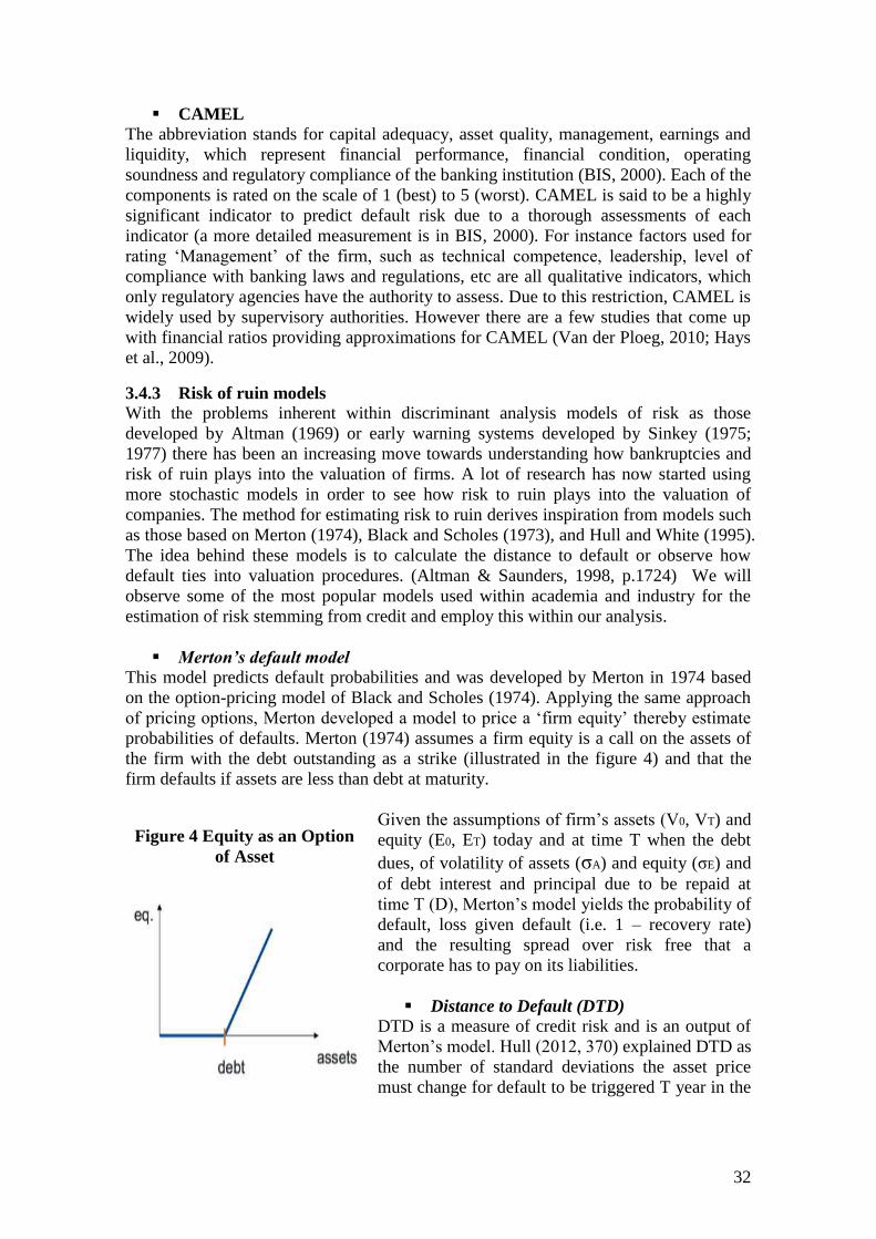
32

CAMEL

The abbreviation stands for capital adequacy, asset quality, management, earnings and

liquidity, which represent financial performance, financial condition, operating

soundness and regulatory compliance of the banking institution (BIS, 2000). Each of the

components is rated on the scale of 1 (best) to 5 (worst). CAMEL is said to be a highly

significant indicator to predict default risk due to a thorough assessments of each

indicator (a more detailed measurement is in BIS, 2000). For instance factors used for

rating ‘Management’ of the firm, such as technical competence, leadership, level of

compliance with banking laws and regulations, etc are all qualitative indicators, which

only regulatory agencies have the authority to assess. Due to this restriction, CAMEL is

widely used by supervisory authorities. However there are a few studies that come up

with financial ratios providing approximations for CAMEL (Van der Ploeg, 2010; Hays

et al., 2009).

3.4.3 Risk of ruin models

With the problems inherent within discriminant analysis models of risk as those

developed by Altman (1969) or early warning systems developed by Sinkey (1975;

1977) there has been an increasing move towards understanding how bankruptcies and

risk of ruin plays into the valuation of firms. A lot of research has now started using

more stochastic models in order to see how risk to ruin plays into the valuation of

companies. The method for estimating risk to ruin derives inspiration from models such

as those based on Merton (1974), Black and Scholes (1973), and Hull and White (1995).

The idea behind these models is to calculate the distance to default or observe how

default ties into valuation procedures. (Altman & Saunders, 1998, p.1724) We will

observe some of the most popular models used within academia and industry for the

estimation of risk stemming from credit and employ this within our analysis.

Merton’s default model

This model predicts default probabilities and was developed by Merton in 1974 based

on the option-pricing model of Black and Scholes (1974). Applying the same approach

of pricing options, Merton developed a model to price a ‘firm equity’ thereby estimate

probabilities of defaults. Merton (1974) assumes a firm equity is a call on the assets of

the firm with the debt outstanding as a strike (illustrated in the figure 4) and that the

firm defaults if assets are less than debt at maturity.

Given the assumptions of firm’s assets (V0, VT) and

equity (E0, ET) today and at time T when the debt

dues, of volatility of assets (σA) and equity (σE) and

of debt interest and principal due to be repaid at

time T (D), Merton’s model yields the probability of

default, loss given default (i.e. 1 – recovery rate)

and the resulting spread over risk free that a

corporate has to pay on its liabilities.

Distance to Default (DTD)

DTD is a measure of credit risk and is an output of

Merton’s model. Hull (2012, 370) explained DTD as

the number of standard deviations the asset price

must change for default to be triggered T year in the

Figure 4 Equity as an Option

of Asset

33

future. DTD has to large enough; the more DTD reduces the more likely the company

becomes default. The formula is as follows:

A challenge in implementing Merton model and its output Merton’s DTD model is the

importance it places in the estimation of the asset market value and asset market

volatility since a firm as a going concern presumably possesses intangible assets and

volatility involves a time series of observed asset values which are hard to determine.

Hence, Merton’s model cannot be applied directly (like Black & Scholes model)

without other methods to estimate the unknown variables. However, literature has

revealed a number of methodologies to estimate these parameters. A few of these

methods are: the volatility restriction method proposed by Rone and Verma (1986),

Jones et al. (1984); the market value proxy method used in Brockman and Turtle (2003),

Eom et al. (2004), the KMV iterative method described in Crosbie and Bohn (2003) and

the Maximum Likelihood Estimate (MLE) developed by Duan (1994). The propositions

have their strengths and weaknesses depending on the underlying assumptions and been

criticized by other researchers. Despite all these, KMV appears to be commercially a

common credit risk assessment (BIS, 2005), moreover, the MLE method according to

Duan and Wang (2012) prevails over other existing methods.

3.4.4 Our chosen measure: Distance to Default

Out of the numerous methods for risk measurement, we chose distance to default. The

reason for doing so depended upon both the ease of implementation in light of data

constraints and the exploratory power of the method. Measurements relying on the

probability of default approximated by different proxies are not our choice because of

data constraints. Methods relying on credit ratings, available via rating agencies could

be used yet they were too general a measure for our analysis and the ratings generally

are subjective to the respective ratings agencies. Among other measures; Altman Z-

score is more applicable to non-financial firms and CAMEL covers a wide range of

quantitative as well as qualitative indicators, which we cannot obtain. If we were to use

proxies to approximate the CAMEL we would need to analyse them in combination

with other risk measures such as credit ratings in order to assure that they reflect the

appropriate risks. Moreover these risk measurements are associated with models having

intrinsic problems such as data measured on discreet intervals or ‘the world not being

linear’. Hence, these reasons lead us to the choice of distance to default. However, we

had to adjust our approach towards the distance to default in order suit our data and this

we discuss in the next chapter.

3.4.5 Factors influencing bank / institutional distress

In conducting this research we employed various ratios as variables to address the

question regarding institutional business models and real estate businesses by observing

their impact upon the distance to default measure we selected. The variables employed

capture various aspects of business model changes and real estate businesses within the

modern financial institutions. Furthermore, these are motivated by the theoretical

framework, which we would address in the following discussion.

The interest in firm distress or default has been hotly investigated throughout time. This

is particularly pronounced with regards to the financial firms, where distress has had

wider systemic effects on the overall economy. However, the work by Beaver (1966)

and Altman (1968) gave this field a proper structure for analysis and has guided

34

research so far. Both Beaver and Altman’s approach towards understanding various

variables associated with bank distress carries on until now despite the changing nature

of models and variables associated with the consequent studies.

The literature about influences on bank distress has evolved by building upon the earlier

studies by Altman and Beaver into even more complex and explanatory variables. The

research evolved by incorporating ratios and measures which address the changing

nature of institutions and businesses. Van Der Ploeg (2010) in his study of the literature

on bank defaults gives a thorough understanding of the framework established by

researchers wherein he indentifies the following risk factors: capital adequacy, asset

quality, management quality, earnings and liquidity, within which the variables studied,

could be clustered into.

The table below taken from Van Der Pleog (2010) explains the various ratios used

within the context of the factors emphasized above within some of the most prominent

literature from 1977- 2008.

The table above depicts that most of the studies within this time period had significant

results for the ratios, which formed a proxy for the risk factors identified as the CAMEL

risk factors.

GCARA = Gross Capital / Adjusted Risk Assets, GCONI = Charge-Offs / (Net Operating Income + Loss Provision), CI2LN = (Commercial and Industrial Loans + Loans to REITs and Mortgage Bankers + Construction Loans + Commercial Real

Estate Loans) / Total Assets, NITA = Net Income / Total Assets, , NWTA = Net Worth / Total Assets, ISFTF = Interest

Sensitive Funds / Total Funds, LATA = Liquid Assets / Total Assets, NCAPTA = (Book Equity + Loan Loss Reserves – Loans 90 Days Past Due - Non-Accruing Loans) / Total Assets, NCOTA = Net Charge-Offs / Total Assets, OVRHDTA = Overhead /

Total Assets, INSLNTA = Loans to Insiders / Total Assets, ROA = Return On Assets, LIQ = (Federal Funds Purchased –

Federal Funds Sold) / Total Assets, CAR = Capital Adequacy Ratio, RMGL = Residential Mortgages / Gross Lending, ELOSS

= Expected Loss based on PD / Gross Lending, CONS = Herfindahl Index for Loan Portfolio, NBLI = Norges Bank’s

Liquidity Indicator, OEOI = Operating Expense / Operating Income, TLTD = Total Loans / Total Deposits, CDR = Total

Domestic Time Deposits / Total Assets, NPCR = (Primary Capital – Nonperforming Loans) / Average Total Assets, TLTA = Total Loans / Total Assets, OHR = Operating Expenses / Average Total Assets, TETA = Total Equity / Total Assets, OROTA =

Other Real Estate Owned / Total Assets, NPLTA = Nonperforming Loans / Total Assets, CSTIN = Cost Inefficiency, TETL =

Total Equity / Total Liabilities, LATL = Liquid Assets / Total Liabilities

Source: Van Der Pleog, 2010. p.10

Table 3 Summary of Factors influencing distress in previous studies

35

However, aside from the more prominent literature within bank distress/default which

focuses on CAMEL ratios, Blundell-Wignall & Roulet (2013) and Igan & Pinheiro

(2009) take a different approach towards the factors determining default as they focus

on business models and impacts from the real estate markets. Blundell-Wignall &

Roulet (2013) in their study of large OECD lending institutions use macro ratios to

observe the presence of systemic influences in bank defaults and balance sheet ratios

which express the core business model of banks which include wholesale funding, gross

market value of derivatives, trading assets, interbank asset ratios. They also account for

the diversity of banking operations by accounting for cross-border revenues and number

of subsidiaries. Hence, their approach towards determinants of default is rather

expansive covering a wider dimension of ratios in line with the global nature of the

financial institutions today. Igan & Pinheiro (2009) do not take such an expansive

approach; however, their focus is more towards ratios gauging the impact of mortgage

lending businesses and real estate markets which is why they include ratios such as

outstanding mortgages, mortgage loan to total assets and non-performing loan ratios.

Hence, our research takes inspiration from these two studies as we study a cross country

market and emphasize on the mortgage lending businesses of financial institutions

therein.

3.5 Research Model

In light of the theoretical framework surrounding Scandinavian mortgage markets and

conditions for bank default, we developed a two-tiered analysis of our primary question.

Figure 5 The Research Model

36

The two-tiered system is inspired by the approach taken by Igan & Pinheiro (2009) in

conducting their analysis of commercial bank exposure to real estate markets within the

United States prior to the financial meltdown of 2008. Our approach, however, looks at

this question with an increase in depth and complexity as compared to Igan & Pinheiro

(2009). This pertains to the fact that we have included specific variables in compliance

with the Scandinavian markets and we have used a more sophisticated approach

towards studying the question with our use of Merton’s Distance to Default model for

estimation of default and wide-range of ratios capturing effects from the mortgage

businesses of the institutions.

The two-tiered approach itself allows us to acquire a profound understanding at both the

individual and the economy-wide level to understand the exposure of real estate markets.

The first tier of analysis involves the determination of factors, which affect the

delinquency rate within bank portfolios. This analysis tries to understand macro and

micro factors behind delinquency within the context of Scandinavian markets over a

chaotic period of 2000-2013. The analysis attempts to provide an understanding on a

wider policy level of the various economic factors affecting delinquency rates.

The second tier concerns the large financial institutions within the three economies and

tries to observe the impact stemming from various balance sheet factors and from their

mortgage businesses. In this tier, we attempt to understand the factors within financial

institution books along with two macro economic factors, housing price and interest

rates, which can lead to distress within the institutions. We measure distress by the

using a distance-to-default measure inspired by Merton (1977) model and in line with

Bottazzi et al. (2011) model for measuring distance to default relying on book values.

This analysis completes our outlook from a risk management perspective as it delves

into specific factors from individual banking books and from mortgage business

segments which can affect an institution. Hence it provides an in-depth understanding of

the risks stemming within the banks credit portfolios from the real estate markets.

The two-tiered analysis, therefore, tries to understand the risks from real estate markets

from both a macro and micro perspective as it attempts to understand macro influences

into the delinquency rates and the impact within institutions of risks to the credit

portfolios from the market.

37

CHAPTER 4: PRACTICAL METHOD

This chapter explains the practical method used in conducting this study. First of all we

draw hypotheses deduced from relevant theories presented in the previous chapter. Then

we present the data collection method along with the computation of proxies. The

chapter ends by a clarification of statistical tests used to analyse the data.

4.1 Hypotheses

The objective of this study is to discover how a volatile real estate market impacts

LMLIs in Scandinavia during the period 2004-2013. In order to do this, two sub-

questions need to be answered:

What are the effects of selected factors on delinquency rate of mortgagors in

Scandinavia during the period 2000-2103?

Does the change in institutional business models and mortgage lending business affect

its distance to default?

4.1.1 Delinquency rate of mortgagors

Our main argument on the possibility of a delinquency among borrowers stems from the

low declining interest rates under a long period and the surge of housing prices

throughout these years. As discussed in the problem background and theoretical

framework, the moves in housing prices does not always match the changes in other

prudential economic factors such as disposable income, household wealth or interest

rates. Therefore the borrower’s probability of delinquency on mortgages becomes more

likely when he/she encounters an income shock or unfavourable changes in loan terms

making it troublesome for keeping up with regular interest payments. Moreover,

macroeconomic shocks, such as rising interest rates or stagnant economies are likely to

have strong impacts on defaults by mortgagors as well. With these arguments we model

the aggregate delinquency rate as a function of the following explanatory variables

aggregate mortgage rate, household debt to disposable income ratio and unemployment

rate while controlling for variables indicating the position of the housing market such as

housing prices, mortgage credit growth outstanding mortgage and the business cycle –

GDP growth, interest rate changes and social benefits. Hence we expect these factors

lead to delinquency of mortgagors noticing that some factors carry a more significant

impact than the others. Stated below are the assumptions and hypotheses with regards to

individual variables.

The first model is:

Delit = β0 + β1*RFit + β2*HPIChngit + β3*Unempit + β4*DebtIncomeit +

β5*SocialBenefitit + β6*GDPgrowthit + β7*MortRateit + β8*OutMortgtit +

β9*Mortgrowthit + Vit

H1-Risk free rate (RF). The risk free rate reflects the monetary policy of the central

bank. A change in risk free rate affects a number of other factors such as mortgage rate,

household income and housing prices. Delinquency is expected to have positive relation

with RF (+). Based on this assumption the first hypothesis is:

Ho: βRF = 0

38

Ha: βRF ≠ 0

Here the βRF indicates the relationship between risk free rate and delinquency rate. The

null hypothesis states that risk free rate does not have an impact on delinquency and the

alternative hypothesis would state the opposite.

H2- House price change (HPIchng). An increase in house price goes together with an

increase in the market value of the house, in our argument this phenomena implies

speculation in the increased value of the property in real estate market and thus we

expect this to have positive impact on delinquency (+). Based on this assumption our

second hypothesis is:

Ho: βHPIChng = 0

Ha: βHPIChng ≠ 0

Here βHPIChng indicates the relationship between the change in house price and

delinquency rate. The null hypothesis states that change in house price does not have an

impact on delinquency and the alternative hypothesis would state the opposite.

H3-Unemployment (Unemp). Unemployment cuts down the income source of

borrowers, which affects their creditworthiness. A high unemployment rate goes in line

with high delinquency rate since more borrowers cannot afford to pay the interests (+).

Based on this assumption our third hypothesis is:

Ho: βUnemp = 0

Ha: βUnemp ≠ 0

Here βUnemp indicates the relationship between unemployment rate and delinquency

rate. The null hypothesis states that unemployment rate does not have an impact on

delinquency and the alternative hypothesis would state the opposite.

H4-Debt/Income ratio (DebtIncome). Household debt to disposable income ratio is

supposed to have a positive relation with delinquency, since the higher the debt burden

is the more economic constraints mortgagors have to bear and thus the chance to fail the

interest payment are significant (+). Based on this assumption our forth hypothesis is:

Ho: βDebtIncome = 0

Ha: βDebtIncome ≠ 0

Here βDebtIncome indicates the relationship between debt and income ratio and

delinquency rate. The null hypothesis states that debt and income ratio does not have an

impact on delinquency and the alternative hypothesis would state the opposite.

H5-Social Benefit (SocialBenefit). A high rate of unemployment benefit might lessen

the debt burden of mortgagors at a certain time, however this implies a high number of

unemployed people, thus this should be positively related to delinquency (+). Based on

this assumption our fifth hypothesis is:

Ho: βSocialBenefit = 0

Ha: βSocialBenefit ≠ 0

39

Here βSocialBenefit indicates the relationship between social benefit and delinquency

rate. The null hypothesis states that social benefit does not have an impact on

delinquency and the alternative hypothesis would state the opposite.

H6-GDP growth (GDPgrowth). GDP growth reflects the healthiness of an economy

overall which places less burden on the household economy and thus less problem of

delinquent loans to the banks. GDP growth expects to be negatively related to

delinquency (-). Based on this assumption our sixth hypothesis is:

Ho: βGDPgrowth = 0

Ha: βGDPgrowth ≠ 0

Here βGDPgrowth indicates the relationship between GDP growth and delinquency

rate. The null hypothesis states that GDP growth does not have an impact on

delinquency and the alternative hypothesis would state the opposite.

H7-Mortgage rate (MortRate). Mortgage rate is the premium the bank charges its

mortgagors. The higher the mortgage rates the harder for mortgagors to fulfil the

interest payments. Thus, mortgage rate is expected to be positively related to

delinquency (+). Based on this assumption our seventh hypothesis is:

Ho: βMortRate = 0

Ha: βMortRate ≠ 0

Here βMortRate indicates the relationship between mortgage rate and delinquency rate.

The null hypothesis states that mortgage rate does not have an impact on delinquency

and the alternative hypothesis would state the opposite.

H8-Outstanding mortgages (OutMortg). This variable is inline with the mortgage

growth. The more outstanding mortgage in the market the more risks involve, hence this

should be positively correlated to DTD (+). Based on this assumption our eighth

hypothesis is:

Ho: βOutMortg = 0

Ha: βOutMortg ≠ 0

Here βOutMortg indicates the relationship between outstanding mortgages and

delinquency rate. The null hypothesis states that outstanding mortgages do not have an

impact on delinquency and the alternative hypothesis would state the opposite.

H9-Mortgage growth (Mortgrowth). This variable corresponds to the change in house

prices, the higher the house price gets the more mortgage grows, hence mortgage

growth should have positive impact on delinquency (+). Based on this assumption our

ninth hypothesis is:

Ho: βMortgrowth = 0

Ha: βMortgrowth ≠ 0

40

Here βMortgrowth indicates the relationship between mortgage growth and delinquency

rate. The null hypothesis states that mortgage growth does not have an impact on

delinquency and the alternative hypothesis would state the opposite.

4.1.2 Distance to default of banks

DTD is used as a proxy for bank distress. To detect banks exposure we model the bank

DTD as a function of these explanatory variables, macro factors, such as default rate,

change in house prices, and interbank interest rate while controlling for factors

indicating the banks business model and their business activities, such as, capital

adequacy liquidity, whole sale funding, interbank assets, net income, derivatives; and

variables accounting for the proportion of mortgage lending institutions in the banks,

such as the proportions of mortgages and revenue. Stated below are the hypotheses with

regards to individual variables.

The second model is:

DTDit = β0 + β1*HPIChngit + β2*Mort2TAit + β3*RWAit + β4*INTTAit +

β5*WSFDTLit + β6*NITAit + β7*L2Dit + β8*Derit + β9*MortGit + β10*Delit +

β11*RevTAit + Vit

H1-House prices change (HPIChng). The variable captures at a certain extent

monetary policy of a country and the credit cycle of asset prices. An increase in house

prices implies gains in the increased value of the house, which leads to a high DTD,

thus DTD is expected to be positively related to ΔHPI (+). Based on this assumption the

first hypothesis is:

Ho: βHPIChng = 0

Ha: βHPIChng ≠ 0

Here βHPIChng indicates the relationship between change in house price and DTD. The

null hypothesis states that change in house price does not have an impact on DTD and

the alternative hypothesis would state the opposite.

H2-Mortgage/Total assets (Mort2TA) Total mortgages of a mortgage company over

total assets of the group represent the proportion of mortgages in the portfolio of the

bank. The larger the mortgage portion is the more vulnerable the bank become, thus

DTD is positively correlated to Mort2TA (+). Based on this assumption the second

hypothesis is:

Ho: βMort2TA = 0

Ha: βMort2TA≠ 0

Here βMort2TA indicates the relationship between the share of mortgages in the group

asset and DTD. The null hypothesis states that the share of mortgage in the group asset

does not have an impact on DTD and the alternative hypothesis would state the

opposite.

H3-RWA. The capital available for risk-weighted assets is a good estimation for the

capacity to absorb risks of banks. A high capital ratio is a good predictor for a far DTD,

thus should have positive relation with DTD (+). Based on this assumption the third

hypothesis is:

41

Ho: βRWA = 0

Ha: βRWA ≠ 0

Here βRWA indicates the relationship between risk weighted asset and DTD. The null

hypothesis states that risk weighted asset does not have an impact on DTD and the

alternative hypothesis would state the opposite.

H4-Interbank Assets/Total assets (INTTA). Banks hold each other’s assets in the

interbank market and can sell these liquid assets in case of liquidity crunch. The ratio is

expected to be positively related to DTD (+). Based on this assumption the forth

hypothesis is:

Ho: βINTTA = 0

Ha: βINTTA ≠ 0

Here βINTTA indicates the relationship between interbank assets and DTD. The null

hypothesis states that interbank assets do not have an impact on DTD and the alternative

hypothesis would state the opposite.

H5-Whole sale funding/Total Liability (WSFTL). This reflects the sources banks use

to finance their liabilities besides deposits from the public. Wholesale funding is short-

term funds and more vulnerable than retail funds in stressed market. DTD is negatively

related to a high level of wholesale funding (-). Based on this assumption the fifth

hypothesis is:

Ho: βWSFTL = 0

Ha: βWSFTL ≠ 0

Here βWSFTL indicates the relationship between wholesale funding and DTD. The null

hypothesis states that wholesale funding does not have an impact on DTD and the

alternative hypothesis would state the opposite.

H6-Net income/Total assets (NITA). The profitability of the banks reflects the ability

to cover losses. Hence DTD is expected to have a positive relation with profitability (+).

Based on this assumption the sixth hypothesis is:

Ho: βNITA = 0

Ha: βNITA≠ 0

Here βNITA indicates the relationship between net income and DTD. The null

hypothesis states that net income does not have an impact on DTD and the alternative

hypothesis would state the opposite.

H7-Loan to deposit ratio (L2D). The proportion of loans as assets as compared to

deposits as liabilities reflects a sound funding of the banks through retail funds, which is

liquid. A high proportion implies the reliance on wholesale funding of the banks. Hence,

this ratio should have positive relation with DTD (+). Based on this assumption the

seventh hypothesis is:

42

Ho: βL2D = 0

Ha: βL2D ≠ 0

Here βL2D indicates the relationship between loan to deposit ratio and DTD. The null

hypothesis states that loan to deposit ratio does not have an impact on DTD and the

alternative hypothesis would state the opposite.

H8-Derivatives/Total assets (Der). Derivatives represent the risk of margin calls in

volatile market, the more derivatives banks hold; the larger the call on capital or the

more the assets become liquid. This ratio is expected to have negative impact on DTD (-

). Based on this assumption the eighth hypothesis is:

Ho: βDer = 0

Ha: βDer ≠ 0

Here βDer indicates the relationship between derivatives and DTD. The null hypothesis

states that derivatives do not have an impact on DTD and the alternative hypothesis

would state the opposite.

H9-Mortgage growth (MortG). The more the mortgages grow, the more the exposure

of banks to these risky assets, therefore mortgage growth is expected to have negative

relation with DTD. Based on this assumption the ninth hypothesis is:

Ho: βMortG = 0

Ha: βMortG≠ 0

Here βMortG indicates the relationship between mortgage growth and DTD. The null

hypothesis states that mortgage growth does not have an impact on DTD and the

alternative hypothesis would state the opposite.

H10-Delinquency (Del). A high number of impaired loans in comparison to the total

mortgages represent a high risk of defaults. DTD is expected to have negative relation

with impaired loans (-). Based on this assumption the tenth hypothesis is:

Ho: βDel = 0

Ha: βDel ≠ 0

Here βDel indicates the relationship between delinquency rate and DTD. The null

hypothesis states that delinquency rate does not have an impact on DTD and the

alternative hypothesis would state the opposite.

H11-Revenue/Total Mortgage (RevMort). The more profitable the mortgage company

is the less financial burden it places on the group or in other words the more financial

funds it contributes to the group, hence this ratio should have positive relationship with

DTD (+). Based on this assumption the eleventh hypothesis is:

Ho: βRevMort = 0

Ha: βRevMort ≠ 0

43

Here βRevMort indicates the relationship between the share of mortgage revenue and

DTD. The null hypothesis states that the share of mortgage revenue does not have an

impact on DTD and the alternative hypothesis would state the opposite.

4.2 Data collection

In this study we utilise micro and macro datasets along with institutional financial

reports from the three countries with yearly frequency. As discussed throughout the text,

our sample includes LMLIs in Sweden, Norway and Denmark representing for the

whole population in Scandinavia. Thirteen banks and LMLIs are selected based on the

market share they capture in each country, which we have discussed in the background

and the countries’ insights. Although the sample is not large, we expect the large market

share pertaining to 90% or above of the institutions within respective markets is

sufficient to reflect the exposure of the mortgage-lending sector to the real estate market.

Table 4 and 5 depict the samples and specific data and data sources used respectively

Table 5 Data and data sources used in the study

Table 4 Banks and LMLIS covered in the study

44

Proxies

The choice of variables and ratios was based on the relevant theories. Among others, the

research by Blundell-Wignall and Roulet (2013) and Igan and Pinheiro (2010) were our

main guides in conducting this research. The variables and ratios we used came from

the bank annual statements including the notes section. However, since not all variables

and ratios were given, we needed to derive and approximate some of them:

Wholesale funding = Liability – Deposits from public – Debt securities issued

Interbank assets = Loans to credit institutions

Delinquency rate = (Impaired loans + Loan losses)/ Total mortgages

Mortgage rate = Representative rates

Interbank rate = Stibor, Oibor, Cibor

RWA = Tier 1 capital ratio

4.3 Computation of DTD

The Merton’s (1977) distance to default model was developed as one of the dynamic

models in order to assess the question of bank contagion. Overall it assumes the bank

equity as a call option on the banks debt holder, whereupon default the equity holder

does not get any pay off where as the entire pay off goes to the writer of the call which

in this case is represented by the debt holder. Furthermore the model involves the

assumption of Brownian motion with a constant drift frequency represented by the

volatility of the assets as described in the earlier chapter.

However within the case of our research we had to modify our approach towards

measuring distance to default since we considered regional subsidiaries of the Nordea

Banking group within Sweden, Norway and Denmark. Along with these subsidiaries we

also considered mortgage companies, which are not actively traded on the financial

markets these include public owned firms such as Lansforsakringar AB, SBAB and

mortgage companies such as Nykredit and BRF. Hence we applied the approach used

by Bottazzi et al. (2011), which is based on a method to find the naïve DD by Bharath

& Shumway (2008).

Bharath and Shumway (2008) explained distance to default as:

Naïve DD=

σ

σ

Where E is the equity market value, F is the face value of debt, T is the time to maturity

assuming that every firm has just a single bond maturing over the T period, rt-1 is the

firm’s stock return over the previous year, and naïve σv represents the volatility of firm

assets which will be computed as follows:

Naive σv =

σ

σ

In this equation the volatility of debt is assumed to be the term in the parenthesis

composed of the volatility of equity (σe), which is an estimate of the Black-Scholes

Merton’s volatility of debt as predicted by Bharath & Shumway (2008, p. 9). However,

Bottazzi et al. (2011) modified this approach by making it suitable to those firms that

were not publicly traded, which we have adopted within our distance to default

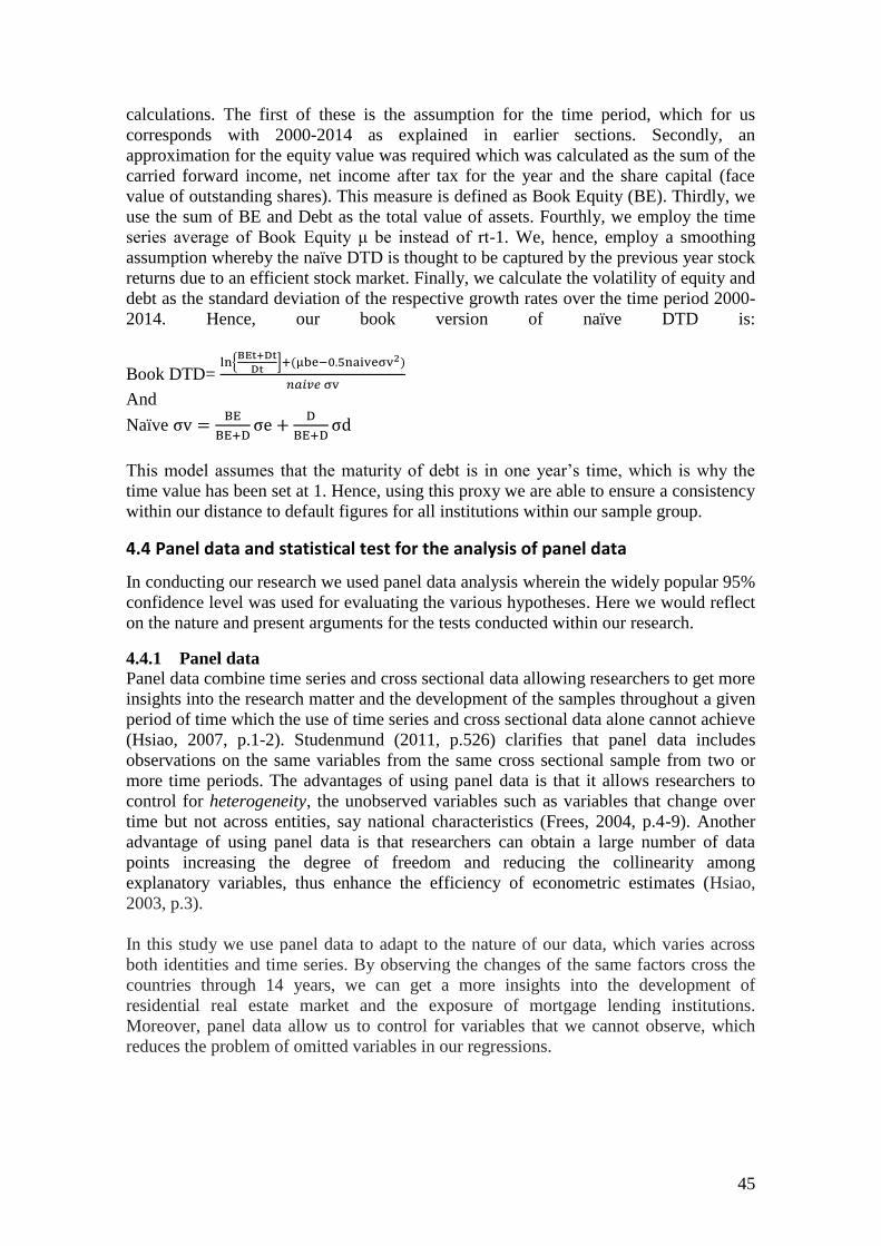
45

calculations. The first of these is the assumption for the time period, which for us

corresponds with 2000-2014 as explained in earlier sections. Secondly, an

approximation for the equity value was required which was calculated as the sum of the

carried forward income, net income after tax for the year and the share capital (face

value of outstanding shares). This measure is defined as Book Equity (BE). Thirdly, we

use the sum of BE and Debt as the total value of assets. Fourthly, we employ the time

series average of Book Equity μ be instead of rt-1. We, hence, employ a smoothing

assumption whereby the naïve DTD is thought to be captured by the previous year stock

returns due to an efficient stock market. Finally, we calculate the volatility of equity and

debt as the standard deviation of the respective growth rates over the time period 2000-

2014. Hence, our book version of naïve DTD is:

Book DTD=

And

Naïve

This model assumes that the maturity of debt is in one year’s time, which is why the

time value has been set at 1. Hence, using this proxy we are able to ensure a consistency

within our distance to default figures for all institutions within our sample group.

4.4 Panel data and statistical test for the analysis of panel data

In conducting our research we used panel data analysis wherein the widely popular 95%

confidence level was used for evaluating the various hypotheses. Here we would reflect

on the nature and present arguments for the tests conducted within our research.

4.4.1 Panel data

Panel data combine time series and cross sectional data allowing researchers to get more

insights into the research matter and the development of the samples throughout a given

period of time which the use of time series and cross sectional data alone cannot achieve

(Hsiao, 2007, p.1-2). Studenmund (2011, p.526) clarifies that panel data includes

observations on the same variables from the same cross sectional sample from two or

more time periods. The advantages of using panel data is that it allows researchers to

control for heterogeneity, the unobserved variables such as variables that change over

time but not across entities, say national characteristics (Frees, 2004, p.4-9). Another

advantage of using panel data is that researchers can obtain a large number of data

points increasing the degree of freedom and reducing the collinearity among

explanatory variables, thus enhance the efficiency of econometric estimates (Hsiao,

2003, p.3).

In this study we use panel data to adapt to the nature of our data, which varies across

both identities and time series. By observing the changes of the same factors cross the

countries through 14 years, we can get a more insights into the development of

residential real estate market and the exposure of mortgage lending institutions.

Moreover, panel data allow us to control for variables that we cannot observe, which

reduces the problem of omitted variables in our regressions.

46

4.4.2 Fixed and Random Effects Models

Among others models, fixed and random models are the two common ones that have

been proposed by a number of econometricians such as Baltagi (2008) or Wooldridge

(2010) as appropriate for panel data analysis.

Fixed effects model

Fixed effect model explores the relationship between a predictor and independent

variables within an entity, such as a country or a company. The model assumes that the

characteristics of an individual entity may cause bias in estimating the predictor and the

independent variables compelling a researcher to control for this. The fixed effects

model works in the way that it allows each cross sectional unit to have a different

intercept to account for the differences between an individual unit and one or more

dummy variables. It also does this in order to account for possible omitted variables that

do not change over time, which might cause bias in estimating the variables coefficients

(Hsiao, 2003, p. 30-33). Using the term ‘fixed effects’ the model assumes the variation

across entities is fixed and correlated with the regressors in the models, which reflect

the correlation between the error term and other variables (2003, p.31). When such a

correlation exists, the researcher would have chosen the wrong model and should apply

random effect model instead.

We chose the fixed effects model for our first question because we were interested in

analyzing the impact of variables that vary over time, such as changes in interest rates,

housing prices, household debt to income ratios, or unemployment rates and the impact

these variables have on the delinquency rates of mortgagors. Furthermore, using the

fixed effect model helps us to explore the relationship between delinquency rate and

other explanatory variables while controlling for possible differences that might exist

within the country, which is in line with our premise regarding the relative similarity

within Scandinavian markets. Moreover, we can disregard the probable correlation of

time-invariant variables since in the model of delinquency rate we have no time

invariant variables.

Random effects model Another option for panel data analysis is using the random effect model. While the fixed

effect model assumes different intercept for each cross sectional unit, the random effect

model assumes the intercept of each cross sectional unit is drawn from a distribution

that is centered around a mean intercept (Wooldridge, 2008, p. 489). By this the model

assumes the variation across entities to be random and uncorrelated with the predictors.

Since the model disregards the possible variations between cross sectional units that can

repeat over time, there is a possibility of omitted variable bias. An advantage of random

effects model researcher can include time invariant variables while in the fixed effects

model, these variables are absorbed by the intercept.

We use the random effects model for our second question since we believe that

variation between entities is significant since the structure of the institutions vary and

because there is correlation between error terms, which we can control via random

effect models.

47

4.4.3 Diagnostics tests

Hausman test

Haumans test (1978) is the only recommended test that can prioritize the choice of fixed

or random effects model. The application of this test is to check whether there is

significant correlation between the error terms or the unobserved specific random

effects and the regressors. The test is simply a comparison of the covariance matrix of

the regressors in the fixed effect model with those in the random effect model given the

null hypothesis that there is no correlation. If there is no statistical significant difference

between the covariance matrixes of the two models, then the correlations of the random

effects with the regressors are statistically insignificant and the fixed effect model

prevails and vice versa.

Testing for time fixed effects As earlier mentioned fixed effects model control for all time invariant differences

between individuals, researcher needs to double check if this is the case. This can be

done by a normal fixed effects regression with the inclusion of all the year dummies to

see if the dummies for all years combined are equal to 0, if they are then no time effect

are needed.

Breusch-Pagan Lagrange Multiple and Pesaran test for cross-section dependence

As discussed earlier the random effects model assumes there is no correlation between

the cross sectional unit and the predictors, we need to test if this is the case and if it is

then heteroskedasticity arising from group-wise differences is the issue at hand. This

happens when the observations of the error term are drawn from a distribution that has

different variance, which causes biased standard errors and leads to biased inference of

the results (Wooldridge, 2008, p. 264). To justify this problem Breusch-Pagan LM test,

which is based on the average squared pairwise correlation coefficients was introduced.

The method behind the test is to first obtain the residuals of the estimated regression

equation, then to run a linear regression with the squared residuals from the original

equation as a function of all the independent variables in that equation (Wooldridge,

2008, p. 273). The null hypothesis is that residual across entities are not correlated. If

the p-value of the test is sufficiently small at significant level, we can reject the null

hypothesis and thus the researcher need to control for heteroskedasticity problem.

Another powerful test to diagnose for random effects is the Pesaran test for cross-

section dependence. The test is based on a simple average of all pairwise correlation

coefficients of the OLS residuals from the individual regressions in the panel (Pesaran,

2004, p.2). The null hypothesis is the residuals are not correlated. The strength of

Pesaran is that it is applicable independent small sample bias of the parameter estimate,

the fixed or random effect residuals will have mean zero provided the disturbances are

symmetrically distributed (Pesaran, 2004, p.6).

Wooldridge test for autocorrelation Serial correlation or autocorrelation refers to correlations among observations taken

over time (Studenmund, 2011, p. 305). Informally it exists when we expect there is an

effect of an independent variable on a dependent variable after a time lag or there are

repeating trends through a certain time span. Serial correlation causes bias standard

errors of the coefficient and R-squared leading to unreliable hypothesis testing

48

(Studenmund, 2011, p. 312-314). To improve this problem we used Wooldridge (2002)

test for autocorrelation in panel data. The method is to analyze how well the lagged

residuals explain the residuals of the original equation. The null hypothesis is that there

is no autocorrelation. If the lagged residuals significantly explain the time’s residuals,

then the null hypothesis of no serial correlation can be rejected.

Hence having discussed the tools, estimators and tests for empirical analysis we can

provide an overview of our empirical model. The first model consists of 3 group

(country) variables of which we set dummy 0 for Sweden, 1 for Norway and 2 for

Denmark and time variable of 14 years from 2000-2013. The second model entails 13

group (banks) variables of which six belong to Sweden, 3 to Norway and 4 to Denmark

and time variable of 10 years from 2004-2013. The time spans in two models are

different due to a lack of data of Sparebank 1 and Lansfosakringar in the first four years.

Below are the two models (for the variable abbreviations, review the hypothesis

section).

Model for delinquency of mortgagors:

Delit = β0 + β1*RFit + β2*HPIChngit + β3*Unempit + β4*DebtIncomeit +

β5*SocialBenefitit + β6*GDPgrowthit + β7*MortRateit + β8*OutMortgtit +

β9*Mortgrowthit + Vit

(Where Vit is the error term, and i, t are indexes for cross sectional unit and time)

Model for distance to default:

DTDit = β0 + β1*HPIChngit + β2*Mort2TAit + β3*RWAit + β4*INTTAit +

β5*WSFDTLit + β6*NITAit + β7*L2Dit + β8*Derit + β9*MortGit + β10*Delit +

β11*RevTAit + Vit

(Where Vit is the error term, and i, t are indexes for cross sectional unit and time)

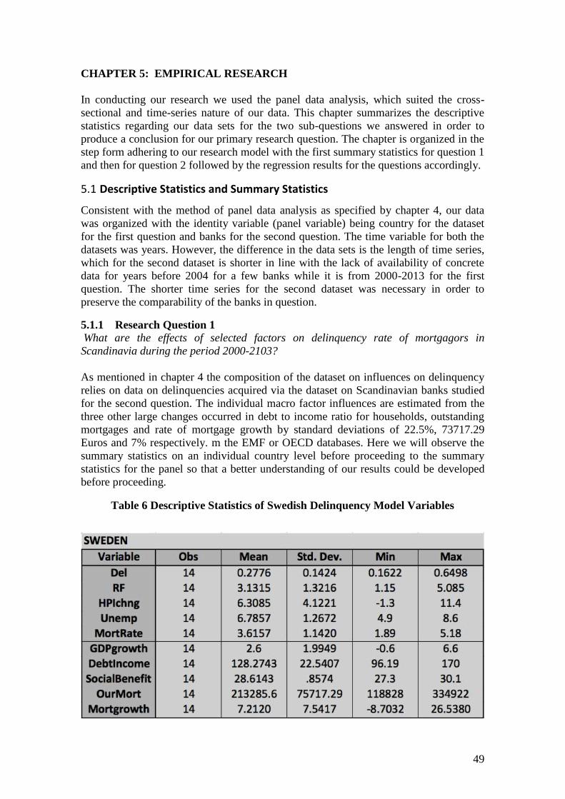
49

CHAPTER 5: EMPIRICAL RESEARCH

In conducting our research we used the panel data analysis, which suited the cross-

sectional and time-series nature of our data. This chapter summarizes the descriptive

statistics regarding our data sets for the two sub-questions we answered in order to

produce a conclusion for our primary research question. The chapter is organized in the

step form adhering to our research model with the first summary statistics for question 1

and then for question 2 followed by the regression results for the questions accordingly.

5.1 Descriptive Statistics and Summary Statistics

Consistent with the method of panel data analysis as specified by chapter 4, our data

was organized with the identity variable (panel variable) being country for the dataset

for the first question and banks for the second question. The time variable for both the

datasets was years. However, the difference in the data sets is the length of time series,

which for the second dataset is shorter in line with the lack of availability of concrete

data for years before 2004 for a few banks while it is from 2000-2013 for the first

question. The shorter time series for the second dataset was necessary in order to

preserve the comparability of the banks in question.

5.1.1 Research Question 1

What are the effects of selected factors on delinquency rate of mortgagors in

Scandinavia during the period 2000-2103?

As mentioned in chapter 4 the composition of the dataset on influences on delinquency

relies on data on delinquencies acquired via the dataset on Scandinavian banks studied

for the second question. The individual macro factor influences are estimated from the

three other large changes occurred in debt to income ratio for households, outstanding

mortgages and rate of mortgage growth by standard deviations of 22.5%, 73717.29

Euros and 7% respectively. m the EMF or OECD databases. Here we will observe the

summary statistics on an individual country level before proceeding to the summary

statistics for the panel so that a better understanding of our results could be developed

before proceeding.

Table 6 Descriptive Statistics of Swedish Delinquency Model Variables

50

The table above shows the summary statistics for Sweden. As observable from the

dataset delinquency in Sweden averaged a 0.28% which is considerably lower for the

tumultuous period in consideration and delinquencies did not increase 0.65% of the total

mortgages given out and the change was not substantial considering the low standard

deviation of 0.14%. The risk free interest rate averages 3.13% with a low standard

deviation of 1.32%. Housing prices changes remains at 6.3% over time period with a

higher standard deviation of 4.12% and a maximum value of 11.4% which highlight a

considerably heated market since this is the change in the average index prices wherein

the base was elevated in 2000. Unemployment in Sweden remains lower than the

European Union average with an average of 6.78% over the time period and hitting a

maximum of 8.6%. Mortgage rate, GDP growth and social benefit as a percentage of

GDP all have a low standard deviation over the time series. The high debt to income

ratio and increase of mortgages highlight the high indebtedness and the heated property

markets within the country.

The table above shows the summary statistics for Norway. Delinquency remains at an

average of 0.76% with a standard deviation of 0.83%, however the range is quite large

compared to other two countries with a maximum value of 2.1% of total mortgages.

Other important highlights are the high spread between house prices changes of 16.8%,

the high indebtedness at 154% with a huge standard deviation of 27% and the large

standard deviation in mortgage growth of 51.75%, which reflects a severely heated

market.

Table 7 Descriptive Statistics of Norwegian Delinquency Model Variables

51

In Denmark the delinquencies remain at an average of 0.23%, which have a standard

deviation 0.165%. Housing price changes had a considerably large spread of 34% which

includes a drop of -12.9% which signifies the crash of the property market. Other

important highlights are the extremely high indebtedness at an average of 236% with an

average deviation of 38% and high mortgage growth average of 6.7%.

Table 8 Descriptive Statistics of Danish Delinquency Model Variables

Figure 6 Panel Summary Statistics

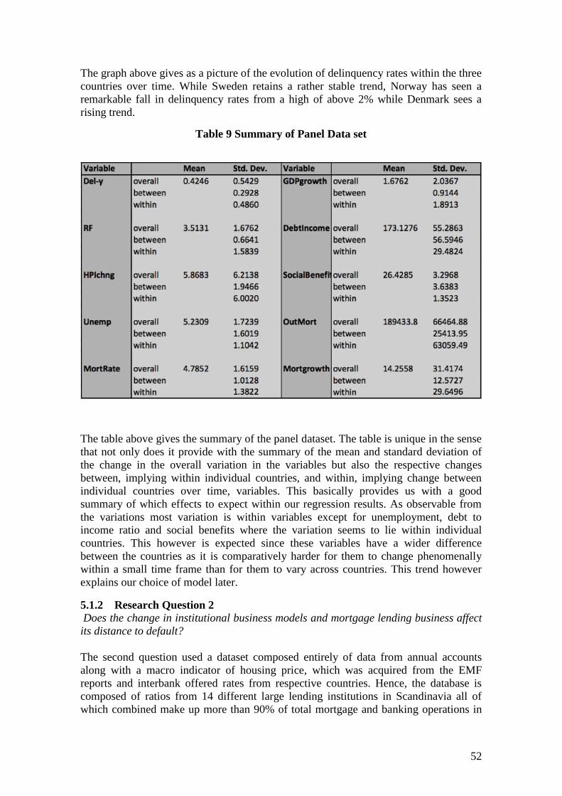
52

The graph above gives as a picture of the evolution of delinquency rates within the three

countries over time. While Sweden retains a rather stable trend, Norway has seen a

remarkable fall in delinquency rates from a high of above 2% while Denmark sees a

rising trend.

The table above gives the summary of the panel dataset. The table is unique in the sense

that not only does it provide with the summary of the mean and standard deviation of

the change in the overall variation in the variables but also the respective changes

between, implying within individual countries, and within, implying change between

individual countries over time, variables. This basically provides us with a good

summary of which effects to expect within our regression results. As observable from

the variations most variation is within variables except for unemployment, debt to

income ratio and social benefits where the variation seems to lie within individual

countries. This however is expected since these variables have a wider difference

between the countries as it is comparatively harder for them to change phenomenally

within a small time frame than for them to vary across countries. This trend however

explains our choice of model later.

5.1.2 Research Question 2

Does the change in institutional business models and mortgage lending business affect

its distance to default?

The second question used a dataset composed entirely of data from annual accounts

along with a macro indicator of housing price, which was acquired from the EMF

reports and interbank offered rates from respective countries. Hence, the database is

composed of ratios from 14 different large lending institutions in Scandinavia all of

which combined make up more than 90% of total mortgage and banking operations in

Table 9 Summary of Panel Data set

53

the market. Here the analysis will be presented briefly for banks individually before

proceeding to summary statistics for the panel.

The Banks The tables below summarize the main bank balance sheet measures including book

distance to default.

Table 10 Summary of Statistics of the Banks Variables

54

These tables have been provided for a comprehensive insight into the institutions’

current business models and their mortgage businesses along with the risk of default

captured by the distance to default (book). Distance to default here should be interpreted

as the number of standard deviations away from a potential default an institution is.

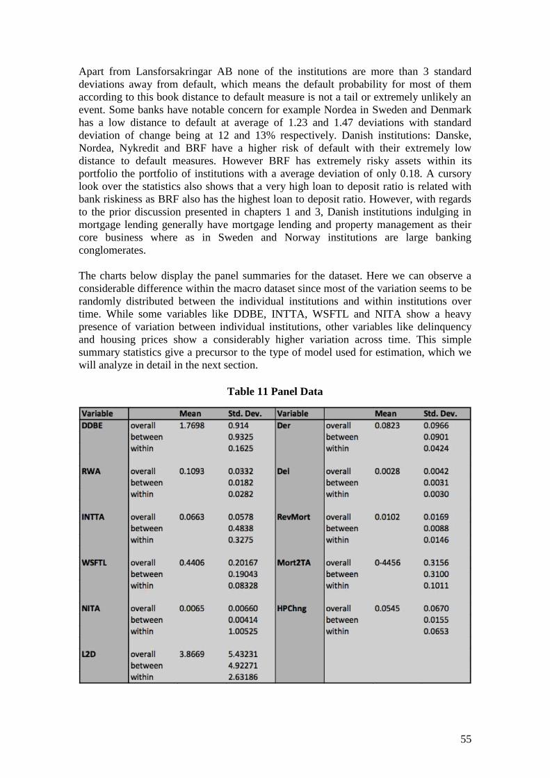
55

Apart from Lansforsakringar AB none of the institutions are more than 3 standard

deviations away from default, which means the default probability for most of them

according to this book distance to default measure is not a tail or extremely unlikely an

event. Some banks have notable concern for example Nordea in Sweden and Denmark

has a low distance to default at average of 1.23 and 1.47 deviations with standard

deviation of change being at 12 and 13% respectively. Danish institutions: Danske,

Nordea, Nykredit and BRF have a higher risk of default with their extremely low

distance to default measures. However BRF has extremely risky assets within its

portfolio the portfolio of institutions with a average deviation of only 0.18. A cursory

look over the statistics also shows that a very high loan to deposit ratio is related with

bank riskiness as BRF also has the highest loan to deposit ratio. However, with regards

to the prior discussion presented in chapters 1 and 3, Danish institutions indulging in

mortgage lending generally have mortgage lending and property management as their

core business where as in Sweden and Norway institutions are large banking

conglomerates.

The charts below display the panel summaries for the dataset. Here we can observe a

considerable difference within the macro dataset since most of the variation seems to be

randomly distributed between the individual institutions and within institutions over

time. While some variables like DDBE, INTTA, WSFTL and NITA show a heavy

presence of variation between individual institutions, other variables like delinquency

and housing prices show a considerably higher variation across time. This simple

summary statistics give a precursor to the type of model used for estimation, which we

will analyze in detail in the next section.

Table 11 Panel Data

56

5.2 Regressions and Tests

The regression tests where carried within the context of individual specific effects in

panel data analysis. In the following explanation we will go through the pre-modelling

diagnostic tests, the model and the selection process.

5.2.1 Regression 1: Delinquency rate of mortgagors

The dataset used for conducting tests in order to answer this question included the

macro-micro dataset explained in the section above. The first test regarding the dataset

was for possible auto-correlation and serial correlations within the set itself. For

conducting this test we used the Lagram Multiplier test approximating a Wooldridge

test for auto-correlation in panel data, as expressed in the earlier chapter.

As displayed by the test H0 was rejected at 5% level and therefore we have some

autocorrelation in the panel data. This clearly implied that we would have to change our

approach towards the models and embrace robust regression models with clustering in

order to address this cross-sectional dependence among the variables. However, this

was not the only problem as the second test for heteroskedasticity, which was conducted

by the modified Wald test for group-wise heteroskedasticity on the simple models

predicted the presence of heteroskedasticity in the simple fixed and random effects

models.

As displayed above the H0 implied that the sigma of all errors squared was equal to the

sigma of all independent variables however at 5% level the H0 was rejected and

therefore hinting the presence of heteroskedasticity within the simple models.

Models and Model Selection As emphasized by the pre-modelling tests the data sets contained heteroskedasticity and

autocorrelation therefore the use of simple models for evaluation was faulty. In

considering alternate tests we had to conduct a robust regression based on the approach

by Newly & West (1987) who developed estimators, which were lag consistent and

therefore usable under the presence of heteroskedasticity and autocorrelation. The

approach we used within the robust regression in this set is loosely depended on Newly

Table 12 Wooldridge test for Regression 1

Table 13 Heteroskedasticity for Regression 1

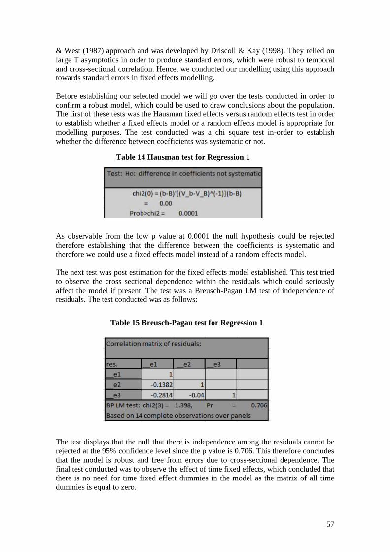
57

& West (1987) approach and was developed by Driscoll & Kay (1998). They relied on

large T asymptotics in order to produce standard errors, which were robust to temporal

and cross-sectional correlation. Hence, we conducted our modelling using this approach

towards standard errors in fixed effects modelling.

Before establishing our selected model we will go over the tests conducted in order to

confirm a robust model, which could be used to draw conclusions about the population.

The first of these tests was the Hausman fixed effects versus random effects test in order

to establish whether a fixed effects model or a random effects model is appropriate for

modelling purposes. The test conducted was a chi square test in-order to establish

whether the difference between coefficients was systematic or not.

As observable from the low p value at 0.0001 the null hypothesis could be rejected

therefore establishing that the difference between the coefficients is systematic and

therefore we could use a fixed effects model instead of a random effects model.

The next test was post estimation for the fixed effects model established. This test tried

to observe the cross sectional dependence within the residuals which could seriously

affect the model if present. The test was a Breusch-Pagan LM test of independence of

residuals. The test conducted was as follows:

The test displays that the null that there is independence among the residuals cannot be

rejected at the 95% confidence level since the p value is 0.706. This therefore concludes

that the model is robust and free from errors due to cross-sectional dependence. The

final test conducted was to observe the effect of time fixed effects, which concluded that

there is no need for time fixed effect dummies in the model as the matrix of all time

dummies is equal to zero.

Table 14 Hausman test for Regression 1

Table 15 Breusch-Pagan test for Regression 1

58

Hence, after the tests the final model is presented below.

As observable from the model it rejects the hypothesis for the F test that the combined

model is equal to zero, which is given by the F statistic showing a probability of lower

than 5% alpha. Thereby there is no problem within this model as it stands and it is

robust. The R-squared is significantly high explaining that the model explains most of

the variation within the variables; therefore further cementing the view that model is

correct. Having established the strength of this robust regression fixed effects model we

would now look at the various hypothesis being tested within the context of this test for

the individual independent variables influencing the delinquency rates in Scandinavia.

The first hypothesis tested was regarding the influence of risk free or interest rates upon

the delinquency rates. At 95% confidence we can reject the null hypothesis that risk free

interest rates do not have an effect on delinquency rates as the p value is 0.04. We can

hence accept the alternate hypothesis as the results show that risk free rates are

positively related to delinquency rates and 1 unit changes in risk free/interest rates

increases delinquency rates by 0.208 units.

The second hypothesis tested within this question was the effect of change in real estate

prices captured by the respective changes in housing price indexes within the countries.

At 95% level of confidence the null hypothesis that the housing price has no effect on

the delinquency rate cannot be rejected therefore implying that the change in housing

prices do not effect delinquency rates as evidenced from the sample where the p value is

high at 0.956.

Table 16 Fixed Effect Model for Regression 1

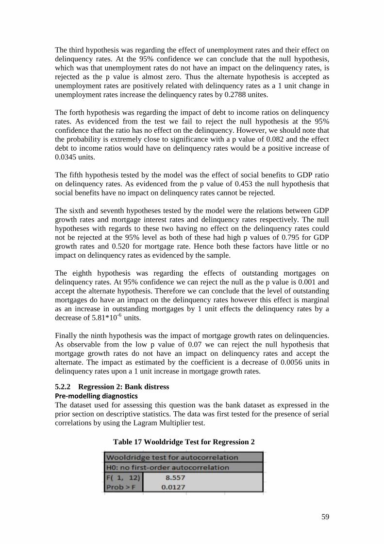
59

The third hypothesis was regarding the effect of unemployment rates and their effect on

delinquency rates. At the 95% confidence we can conclude that the null hypothesis,

which was that unemployment rates do not have an impact on the delinquency rates, is

rejected as the p value is almost zero. Thus the alternate hypothesis is accepted as

unemployment rates are positively related with delinquency rates as a 1 unit change in

unemployment rates increase the delinquency rates by 0.2788 unites.

The forth hypothesis was regarding the impact of debt to income ratios on delinquency

rates. As evidenced from the test we fail to reject the null hypothesis at the 95%

confidence that the ratio has no effect on the delinquency. However, we should note that

the probability is extremely close to significance with a p value of 0.082 and the effect

debt to income ratios would have on delinquency rates would be a positive increase of

0.0345 units.

The fifth hypothesis tested by the model was the effect of social benefits to GDP ratio

on delinquency rates. As evidenced from the p value of 0.453 the null hypothesis that

social benefits have no impact on delinquency rates cannot be rejected.

The sixth and seventh hypotheses tested by the model were the relations between GDP

growth rates and mortgage interest rates and delinquency rates respectively. The null

hypotheses with regards to these two having no effect on the delinquency rates could

not be rejected at the 95% level as both of these had high p values of 0.795 for GDP

growth rates and 0.520 for mortgage rate. Hence both these factors have little or no

impact on delinquency rates as evidenced by the sample.

The eighth hypothesis was regarding the effects of outstanding mortgages on

delinquency rates. At 95% confidence we can reject the null as the p value is 0.001 and

accept the alternate hypothesis. Therefore we can conclude that the level of outstanding

mortgages do have an impact on the delinquency rates however this effect is marginal

as an increase in outstanding mortgages by 1 unit effects the delinquency rates by a

decrease of 5.81*10-6

units.

Finally the ninth hypothesis was the impact of mortgage growth rates on delinquencies.

As observable from the low p value of 0.07 we can reject the null hypothesis that

mortgage growth rates do not have an impact on delinquency rates and accept the

alternate. The impact as estimated by the coefficient is a decrease of 0.0056 units in

delinquency rates upon a 1 unit increase in mortgage growth rates.

5.2.2 Regression 2: Bank distress

Pre-modelling diagnostics The dataset used for assessing this question was the bank dataset as expressed in the

prior section on descriptive statistics. The data was first tested for the presence of serial

correlations by using the Lagram Multiplier test.

Table 17 Wooldridge Test for Regression 2

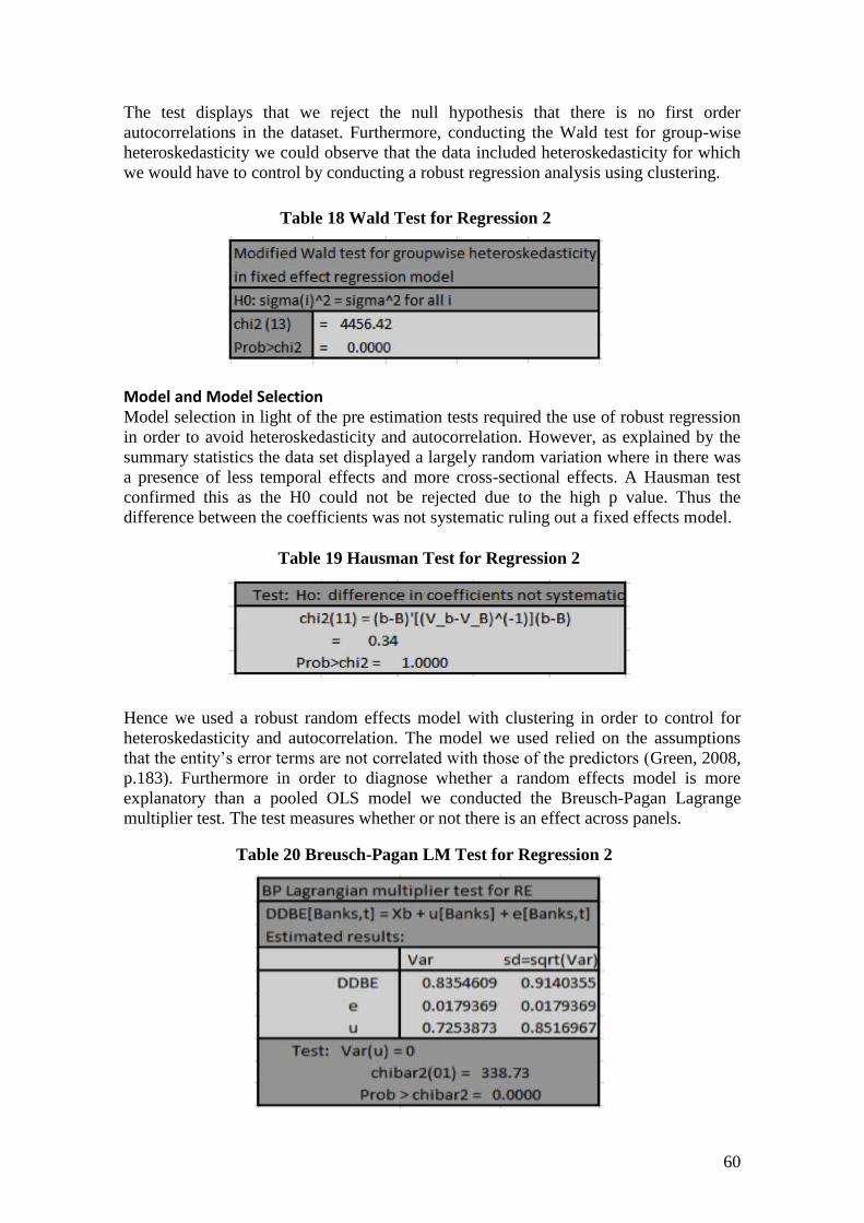
60

The test displays that we reject the null hypothesis that there is no first order

autocorrelations in the dataset. Furthermore, conducting the Wald test for group-wise

heteroskedasticity we could observe that the data included heteroskedasticity for which

we would have to control by conducting a robust regression analysis using clustering.

Model and Model Selection Model selection in light of the pre estimation tests required the use of robust regression

in order to avoid heteroskedasticity and autocorrelation. However, as explained by the

summary statistics the data set displayed a largely random variation where in there was

a presence of less temporal effects and more cross-sectional effects. A Hausman test

confirmed this as the H0 could not be rejected due to the high p value. Thus the

difference between the coefficients was not systematic ruling out a fixed effects model.

Hence we used a robust random effects model with clustering in order to control for

heteroskedasticity and autocorrelation. The model we used relied on the assumptions

that the entity’s error terms are not correlated with those of the predictors (Green, 2008,

p.183). Furthermore in order to diagnose whether a random effects model is more

explanatory than a pooled OLS model we conducted the Breusch-Pagan Lagrange

multiplier test. The test measures whether or not there is an effect across panels.

Table 18 Wald Test for Regression 2

Table 20 Breusch-Pagan LM Test for Regression 2

Table 19 Hausman Test for Regression 2

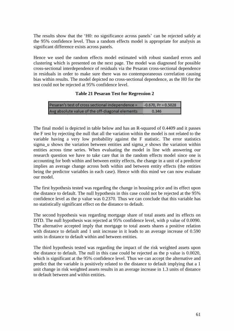
61

The results show that the ‘H0: no significance across panels’ can be rejected safely at

the 95% confidence level. Thus a random effects model is appropriate for analysis as

significant difference exists across panels.

Hence we used the random effects model estimated with robust standard errors and

clustering which is presented on the next page. The model was diagnosed for possible

cross-sectional interdependence of residuals via the Pesaran cross-sectional dependence

in residuals in order to make sure there was no contemporaneous correlation causing

bias within results. The model depicted no cross-sectional dependence, as the H0 for the

test could not be rejected at 95% confidence level.

The final model is depicted in table below and has an R-squared of 0.4409 and it passes

the F test by rejecting the null that all the variation within the model is not related to the

variable having a very low probability against the F statistic. The error statistics

sigma_u shows the variation between entities and sigma_e shows the variation within

entities across time series. When evaluating the model in line with answering our

research question we have to take care that in the random effects model since one is

accounting for both within and between entity effects, the change in a unit of a predictor

implies an average change across both within and between entity effects (the entities

being the predictor variables in each case). Hence with this mind we can now evaluate

our model.

The first hypothesis tested was regarding the change in housing price and its effect upon

the distance to default. The null hypothesis in this case could not be rejected at the 95%

confidence level as the p value was 0.2370. Thus we can conclude that this variable has

no statistically significant effect on the distance to default.

The second hypothesis was regarding mortgage share of total assets and its effects on

DTD. The null hypothesis was rejected at 95% confidence level, with p value of 0.0090.

The alternative accepted imply that mortgage to total assets shares a positive relation

with distance to default and 1 unit increase in it leads to an average increase of 0.590

units in distance to default within and between entities.

The third hypothesis tested was regarding the impact of the risk weighted assets upon

the distance to default. The null in this case could be rejected as the p value is 0.0020,

which is significant at the 95% confidence level. Thus we can accept the alternative and

predict that the variable is positively related to the distance to default implying that a 1

unit change in risk weighted assets results in an average increase in 1.3 units of distance

to default between and within entities.

Table 21 Pesaran Test for Regression 2

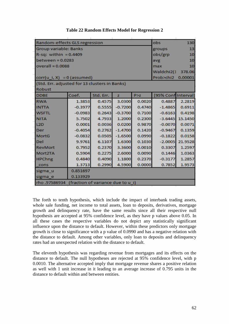
62

The forth to tenth hypothesis, which include the impact of interbank trading assets,

whole sale funding, net income to total assets, loan to deposits, derivatives, mortgage

growth and delinquency rate, have the same results since all their respective null

hypothesis are accepted at 95% confidence level, as they have p values above 0.05. In

all these cases the respective variables do not depict any statistically significant

influence upon the distance to default. However, within these predictors only mortgage

growth is close to significance with a p value of 0.0990 and has a negative relation with

the distance to default. Among other variables, only loan to deposits and delinquency

rates had an unexpected relation with the distance to default.

The eleventh hypothesis was regarding revenue from mortgages and its effects on the

distance to default. The null hypotheses are rejected at 95% confidence level, with p

0.0010. The alternative accepted imply that mortgage revenue shares a positive relation

as well with 1 unit increase in it leading to an average increase of 0.795 units in the

distance to default within and between entities.

Table 22 Random Effects Model for Regression 2

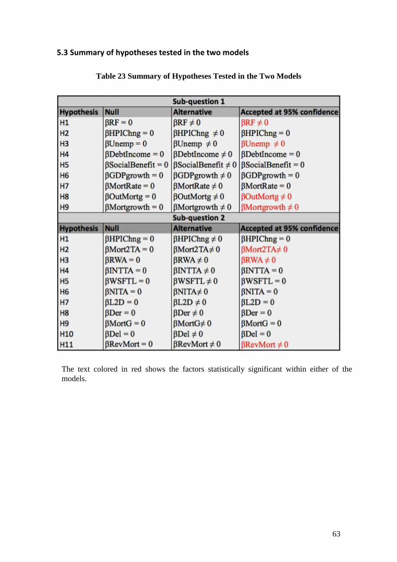
63

5.3 Summary of hypotheses tested in the two models

Table 23 Summary of Hypotheses Tested in the Two Models

The text colored in red shows the factors statistically significant within either of the

models.

64

CHAPTER 6: DATA ANALYSIS

We would now tie in our empirical findings with the theoretical framework established

in chapters 2-4 in order to present a discussion and an eventual answer towards our

primary research question. This chapter also discusses the results from the previous

chapter in light of the prior literature. The chapter first goes over the two sub-questions

and hypotheses developed within these two questions, and then it concludes with a

discussion on the primary research question.

6.1. Research Question 1

What are the effects of selected factors on delinquency rate of mortgagors in

Scandinavia during the period 2000-2103?

In answering this question we used a fixed effects model where in we assessed the

impact of individual entities over time controlling for within entity effects. The model

used was a robust fixed effects regression with Driscoll & Kraay standard errors to

control for heteroskedasticity and autocorrelation. The final model developed was:

Delit = β0 + β1*RFit + β2*HPIChngit + β3*Unempit + β4*DebtIncomeit +

β5*SocialBenefitit + β6*GDPgrowthit + β7*MortRateit + β8*OutMortgtit +

β9*Mortgrowthit + Vit

The equation was robust with a high R-squared of 0.7865 and the non model related

variation in the model is fairly low as displayed below in the predicted alphas, which

indicate non model related variation:

Hence having established the strengths of the model we can now analyze the predictors

and the individual hypotheses.

6.1.1 Interpretations of individual hypotheses

H1: Risk free interest rate

Our results indicated that the risk free interest rate shares a fairly strong positive relation

with the delinquency rates as an increase in 1 unit of the risk free rate results in

increasing delinquency by 0.208 units and this result is significant at the 95%

confidence level with a p value of 0.04. This result is in line with our expectations as

established in chapter 4 since the risk free rate is the basis rate upon which banks at

their interest rates and it also is the standard upon which changes are made on other

lending rates on loans and mortgages. Therefore as displayed by the results and our

intuition the rate increases the interest burden on individuals thereby increasing the rate

of delinquency on mortgage loans. This is in contrast to Igan & Pinhero (2009) who

established a surprisingly negative relation between delinquency rates and interest rates.

Hence, we believe our results reflect a fairly appropriate picture in line with our

Table 24 Alpha Estimation for Regression 1

65

intuitions and the grounded theory behind interest rates and paybacks on mortgages.

However, the results are in line with Andersson & Wilhelmsson’s (2009) inquiry into

Swedish housing markets as they discovered a significant positive relation between

delinquencies and interest rate increases. Therefore, we believe the Scandinavian

market shows difference from the one in the US within this regard.

H2: Change in Housing Prices

Our results displayed a negative yet not a significant relation between the housing price

changes and delinquency rates this is in line with Igan & Pinhero (2009) who also were

not able to establish any significant relation between housing price changes and

delinquencies. Possible reasons for a lack of significance of housing prices maybe as

explained by the research conducted by Sorenson (2013), Browne et al. (2013) and Diaz

& Prado (2011). Sorenson (2013) elaborated that in order to calculate the risk or the

potential effects from changes in housing prices the use of user cost of housing should

be employed rather than simple changes within the housing prices. Browne et al (2013)

argued a similar case when they used the user cost of housing rather than the changing

housing prices in order to study the effects on delinquency and default rates in Ireland.

Diaz & Prado (2011) made a case in their study for the US Federal Reserve using the

user cost measure rather than change in housing prices as they argued the need to use

the utility derived from the housing asset rather than just a market price change

reflecting expectations.

H3: Unemployment Rate

Unemployment rates have a fairly significant relation between delinquency rates, which

is large and positive. This is displayed by the low p value at 0.0001 and a high

coefficient of 0.279, which implies a fairly strong impact of this predictor on the

response. This result is in line with our intuition and with the ability to pay hypothesis

and confirms the findings from Igan & Pinhero (2009) and Serrano (2005) that the

ability to pay hypothesis confirms that delinquency rates would rise in the case of rising

unemployment as mortgagors’ ability to payback mortgages is restricted. Andersson &

Wilhemsson (2009) also discovered a significant positive relation between the

unemployment rate and delinquency rates in Sweden. This further cements the ability to

pay hypothesis that despite differences across economies with regards to welfare

payments unemployment is a strong predictor of delinquencies.

H4: Debt to Income ratio

This predictor had a positive relation with the delinquency rates yet it was not

significant on the 95% level. However, with a p value of 0.08 we expect that a larger

time series might have given a more significant relationship between this predictor but

within our sample it does not predict a significant influence on the delinquency rates.

Bhutta (2012) and Sorenson (2013) both depict that debt to income ratios indeed

influence delinquencies positively as they reduce the mortgagors’ ability to make good

on his debts. Thus, we believe that our results are just a reflection of our smaller time

series.

H5: Social Benefits

The predictor was established keeping in line with Finansinspektionen’s (Swedish

Mortgage Market, 2013) concern regarding the impact of decreasing welfare payments

upon possible rising delinquency rates in the future. However our results indicate no

significant relationship between social benefits payments and delinquency rates. The

66

reason for this might be assumption errors as the only available proxy we could find for

welfare payments was the OECD average social benefit as a percentage of GDP, which

might be a fairly weak predictor of welfare payments.

H6: GDP growth

The GDP growth is an indicator of economic progress within a country and therefore

establishes the total consumption; production, imports, government expenditure and

exports in an economy hence can be a good proxy for the wealth of the individuals or

the expectations of rise of income and wealth. However within our tests as in those

conducted by Igan & Pinhero (2009) on residential mortgages we find no significant

relation between GDP growth and delinquency rate on mortgages.

H7: Mortgage Rate

The test results for mortgage rates were surprising in the sense that it did not have any

significance at 95% confidence level and had a negative relation with delinquency rates.

This however is similar to the findings of Igan & Pinhero (2009) who could not

establish a significant impact of mortgages rates upon delinquency rates. A reason for

this might reflect from the fact that there is a major difference in fixed and variable rates.

Finansinspektion (2013) and Allen et al. (2004) emphasize in the studies of Swedish

and Danish mortgage markets about the change in the popularity of fixed and variable

mortgage rates with then last decade. Thus, in recent times both types of rates have been

used although fixed rates have dominated within Denmark and Sweden; in Norway

variable rates still dominate therefore making this average mortgage rate a rather weak

proxy for the prevailing rates in the market.

H 8 & H9: Outstanding mortgages and mortgage growth

These two predictors concerned more the institutions and the types of individuals

increasing their share in the mortgage market than an individuals’ influence on

delinquency. Both have a statistically significant impact on delinquency rates as

displayed by the p values 0.001 and 0.007 on outstanding mortgages and mortgage

growth rates respectively. This establishes a rather surprising result as both have

depicted a negative relation with respect to delinquency. This is in conflict with the

study conducted by Igan & Pinhero who did not find any significant relationship

between outstanding real estate mortgages and delinquencies on residential real estate

mortgages. The possible reason for a negative relation between both these indicators

might be an indication of the increasing protections being offered in case of

delinquencies and defaults whereby in Denmark the financial supervision authority

takes over the mortgages and in Sweden delinquencies are secured by the government

guarantees as expressed by Finansinpektionen (Swedish Mortgage Market, 2013) and

Admunsen & Art (2005).

6.1.2 Conclusion on Sub Question 1

What are the effects of selected factors on delinquency rate of mortgagors in

Scandinavia during the period 2000-2103?

In trying to establish the answer to this question we looked at possible predictors of

delinquency rates, as specified by literature, across the time series from 2000 to 2013 in

the three Scandinavian economies. The results depicted that the interest rates,

unemployment rates, outstanding mortgages and mortgage growth rates are fairly strong

determinants of delinquency rates. Debt to income, however, is also closely related to

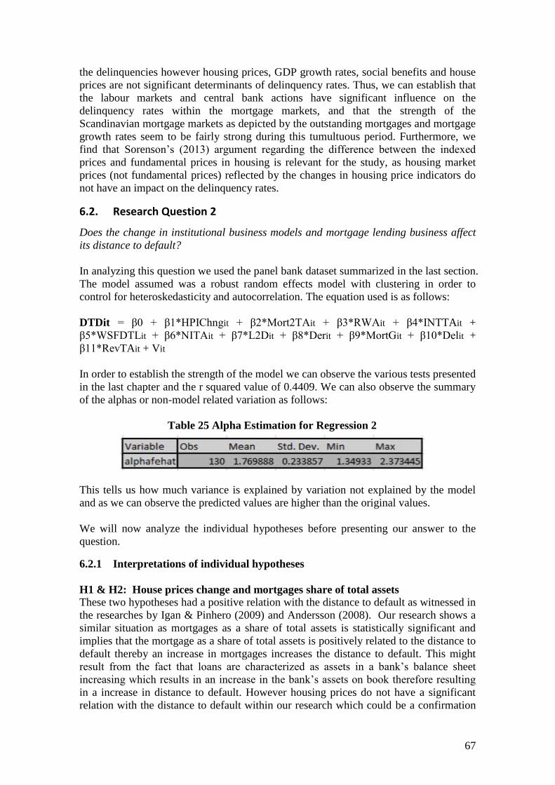
67

the delinquencies however housing prices, GDP growth rates, social benefits and house

prices are not significant determinants of delinquency rates. Thus, we can establish that

the labour markets and central bank actions have significant influence on the

delinquency rates within the mortgage markets, and that the strength of the

Scandinavian mortgage markets as depicted by the outstanding mortgages and mortgage

growth rates seem to be fairly strong during this tumultuous period. Furthermore, we

find that Sorenson’s (2013) argument regarding the difference between the indexed

prices and fundamental prices in housing is relevant for the study, as housing market

prices (not fundamental prices) reflected by the changes in housing price indicators do

not have an impact on the delinquency rates.

6.2. Research Question 2

Does the change in institutional business models and mortgage lending business affect

its distance to default?

In analyzing this question we used the panel bank dataset summarized in the last section.

The model assumed was a robust random effects model with clustering in order to

control for heteroskedasticity and autocorrelation. The equation used is as follows:

DTDit = β0 + β1*HPIChngit + β2*Mort2TAit + β3*RWAit + β4*INTTAit +

β5*WSFDTLit + β6*NITAit + β7*L2Dit + β8*Derit + β9*MortGit + β10*Delit +

β11*RevTAit + Vit

In order to establish the strength of the model we can observe the various tests presented

in the last chapter and the r squared value of 0.4409. We can also observe the summary

of the alphas or non-model related variation as follows:

This tells us how much variance is explained by variation not explained by the model

and as we can observe the predicted values are higher than the original values.

We will now analyze the individual hypotheses before presenting our answer to the

question.

6.2.1 Interpretations of individual hypotheses

H1 & H2: House prices change and mortgages share of total assets

These two hypotheses had a positive relation with the distance to default as witnessed in

the researches by Igan & Pinhero (2009) and Andersson (2008). Our research shows a

similar situation as mortgages as a share of total assets is statistically significant and

implies that the mortgage as a share of total assets is positively related to the distance to

default thereby an increase in mortgages increases the distance to default. This might

result from the fact that loans are characterized as assets in a bank’s balance sheet

increasing which results in an increase in the bank’s assets on book therefore resulting

in a increase in distance to default. However housing prices do not have a significant

relation with the distance to default within our research which could be a confirmation

Table 25 Alpha Estimation for Regression 2

68

of Sorenson’s (2013) research that fundamental housing prices derived from the user

cost model of housing (explained in chapter 3) rather than market house prices affect

economy and institutions.

H3: RWA

The model displays that the risk weighted assets have a statistically significant (p value

0.0020) and positive average relation across identity and time with distance to default.

This is an important finding which contradicts the research of Wignall & Roulet (2013)

who using a time fixed model depicted that risk weighted assets have no significant

relation with the distance to default and conclude that the Basel regulation have not led

to a risk mitigation in bank portfolios. Our result however confirms the research by Van

der ploeg (2010) and Anderssen (2009) who confirmed that the regulation mechanism

developed under the Basel regulatory framework is working in mitigating the risk

within the portfolios of financial institutions. This is reflected by our test where in the

rise in risk weighted assets by one unit increases the average book distance to default by

1.385 units thereby having a considerable effect on the safety of the banks. However,

we should recognize the fact that we have used a different model and proxy for distance

to default and the results could reflect a possible distinction between book and market

oriented measures.

H4 & H5: Interbank trading assets and whole–sale funding

As elaborated by Wignall and Roulet (2013) the relation the relation between interbank

trading assets and whole-sale funding towards distance to default is negative. This is

confirmed by our findings however we find that this result is statistically insignificant

when considering the book distance to default for Scandinavia conflicting with Wignall

and Roulet (2013). This might be a reflection of the dataset constraints or the predictive

value by the distance to default is measured.

H6 & H7: Net income to trading assets and loan to deposit ratios

These two predictors do not give a statistically significant relationship towards the

distance to default and hence show no relation with the changes over time and over

different banks. Igan & Pinhero (2009) saw a similar result within their research as both

these measures failed to give a statistically meaningful impact on distance to default

measures adopted therein. However, Martin (1977), Avery & Hanweck (1984) and

Barth et al. (1985) all discovered that both of these measures to had significant

relationships thereby underscoring that a difference might exist because of the bank

distance to default measure used based on book values and based on the market values.

Furthermore, all three of the studies used a logit model rather than a panel random

effects model, which could explain the possible divergence.

H8 & H9: Derivatives and growth of mortgage portfolios

As observable from Wignall and Roulet (2013), Igan & Pinhero (2009) and Hays et al

(2009) both these factors are negatively related to the distance to default. We observed s

similar relation as the rise in derivatives as a share of assets and growth of mortgage

portfolios are increasingly characterized by increasing the riskiness of a financial

institution. However within our tests we found that the relation was statistically

insignificant, which can be a reflection of the limitations imposed by our dataset

constraints.

H10 & H11: Delinquencies and mortgage revenue

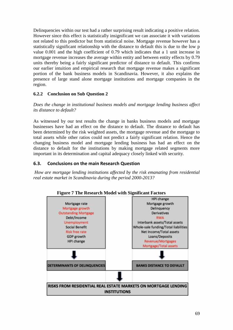
69

Delinquencies within our test had a rather surprising result indicating a positive relation.

However since this effect is statistically insignificant we can associate it with variations

not related to this predictor but from statistical noise. Mortgage revenue however has a

statistically significant relationship with the distance to default this is due to the low p

value 0.001 and the high coefficient of 0.79 which indicates that a 1 unit increase in

mortgage revenue increases the average within entity and between entity effects by 0.79

units thereby being a fairly significant predictor of distance to default. This confirms

our earlier intuition and empirical research that mortgage revenue makes a significant

portion of the bank business models in Scandinavia. However, it also explains the

presence of large stand alone mortgage institutions and mortgage companies in the

region.

6.2.2 Conclusion on Sub Question 2

Does the change in institutional business models and mortgage lending business affect

its distance to default?

As witnessed by our test results the change in banks business models and mortgage

businesses have had an effect on the distance to default. The distance to default has

been determined by the risk weighted assets, the mortgage revenue and the mortgage to

total assets while other ratios could not predict a fairly significant relation. Hence the

changing business model and mortgage lending business has had an effect on the

distance to default for the institutions by making mortgage related segments more

important in its determination and capital adequacy closely linked with security.

6.3. Conclusions on the main Research Question

How are mortgage lending institutions affected by the risk emanating from residential

real estate market in Scandinavia during the period 2000-2013?

Figure 7 The Research Model with Significant Factors

70

In answering this question, we have tried to establish a two tiered approach. One of

which addresses the borrower side and the other the lender side of the real estate market

in Scandinavia. Since most of the institutions used in the study are either major

mortgage companies or banks controlling the major share of real estate and mortgage

lending businesses, we could gather the key insights into answering this question by our

two sub questions. The delinquency rate analysis provided us with major determinants

of delinquency as prescribed by theory and therefore an insight into the borrower side of

the mortgage market. This analysis answers the question by providing us with the key

determinants of delinquency, as prescribed by theory, which were interest rates,

unemployment rates, mortgage growth and outstanding mortgages as well as an almost

significant impact from the debt to income ratios. Hence, within the studied time period

delinquency rates on mortgages have been affected by the changing macro and micro

conditions elucidating the effect from the borrower side on the institutions, due to

changing market conditions. This is seen from the increase in mortgage lending

affecting delinquency, an increased risk from macro shocks such as unemployment and

interest rate hikes, and a spike in indebtedness among individuals witnessed by the large

debt to income ratios.

The second aspect of the question concerns whether factors affecting institutional

distress are affected by the residential real estate market conditions. In answering this

question we used our sub-question two with the analysis on the determinants of distance

to default among banks and lending institutions in Scandinavia. The analysis displays

the importance of mortgage share of total assets, revenue from mortgages and core tier

one ratio as the most significant determinants of distance to default during this period in

Scandinavia. Additionally, summary statistics also show increasing loan to deposit

ratios, a larger share of derivative assets and a growth in mortgage portfolios

characterizing the latter part of the time series. This essentially depicts a changing

nature of the businesses. However, over the course of our time series, institutions have

also witnessed a significant impact from changing real estate market conditions as their

mortgage portfolios have increasingly expanded and acquired importance in

determining their risk of distress. Furthermore, the very nature of mortgage lending

institutions has changed over the course of this tumultuous period reflecting a rising

share in new risky instruments and increasing reliance on mortgage lending.

Hence, we can safely conclude that mortgage lending institutions have been affected by

the residential real estate markets between 2000 and 2013. This is due to the changing

characterization of the risks facing their customers, which are transferred onto them via

delinquency and through the changing nature of their businesses. However what

remains to be seen is whether this effect creates opportunities and spurs growth or

whether it manifests troubles and creates major problems.

71

CHAPTER 7: CONCLUSION

The chapter concludes our research by presenting a discussion on the quality of the

research followed by concluding arguments, contributions and recommendations, and

suggestions for further research.

7.1 The credibility of research findings

The quality of a research relies on the following three criterions – reliability, validity

and generalizability (Bryman & Bell, 2012, p. 157-166).

7.1.1 Reliability

This criterion concerns the issue of consistency of the measures. The criterion delves

upon questions such as whether data collection and data analysis are reliable, whether

the measures yield the same results as those by other researchers and whether the data

was transparent and made sense (Bryman & Bell, 2012, p. 157; Saunders et al, 2011, p.

156). The data used in our study comes from internationally reliable databases, which

include the EMF, Eurostat, Thomson Reuters DataStream, OECD databases and

published annual reports of the institutions concerned. The credibility of these sources is

not questionable since they are abundantly used, cited and scrutinized since they are

used for research, policy making and analysis globally. Moreover we have stated clearly

the indicators used in the study and elaborated upon the methods used in computing

them associating them with the corresponding theories. We have also explained the

procedure for the data analysis and compared these to prior research. For these reasons,

we can safely conclude that it does not matter who collects the data since following the

same framework under same time frame, the data should remain the same. Due to this

transparency in data collection and analysis, we can say that our research is replicable

by other researchers since we have clearly outlined the step by step procedure we

followed and highlighted all the tests and estimators employed within the research in

our practical method and empirical research sections. Furthermore, we employed Stata

(stata.com) as a statistical tool to detect the relationships between the variables. The

software is constructed with standard setups of data input as well as output, therefore we

have to strictly adapt to the system and the same for other researchers, and hence the

outcome of the test should be consistent for all researchers. In particular, our research

would not have problem with ‘subject and participant bias’, which asserted by Saunders

et al. (2012, p157) as the inconsistency in the responses of participants. Our quantitative

study relies purely on public statistics, which eliminate the possibility of subjectivity

and participant bias.

7.1.2 Validity

Validity refers to the issue of a concept actually measuring that concept (Bryman & Bell,

2012. p. 159). This criterion questions the causal effect between a dependent variable

and independent variables, and whether this relation is credible rather than being a

response to other factors (2012, 42). In response to the question we based our findings

on facts and theories extracted from peered reviewed articles to state the causal effect.

We interpreted the effect in the light of computational statistical tests with robust

regression to control for any estimation errors causing bias. The causal effect in the first

model between delinquencies and the macro and micro factors stem from the nature of

the countries’ economies, their real estate market conditions and the creditworthiness of

72

the households. The causal effect for the second model is between bank distress and

other accounting factors as prescribed by previous research, outlined in the theoretical

framework. Within the given theoretical framework, accessible data and consequent

analysis was conducted by comparing the results with those of other studies. Hence, our

research can be seen valid within the domains of this criterion.

7.1.3 Generalizability

Generalizability is considered as the external validity of a research. External validity

deals with the question that whether the result of the research can be generalised beyond

the specific research concept (2012, p. 43). As a response to this question we can state

that our sample data, regarding the institutional factors, is representative for banks and

mortgage lending institutions in each of the countries studied as prescribed by prior

studies. These studies are highlighted within the practical methodology. One could

question the number of observation within each of the models, 42 observations for the

first model and 130 for the second, as being fewer than necessary to achieve

generalizability. We would, however, retort by reasoning that the mortgage lending

institutions in the study capture most of the residential real estate market in each of the

respective countries mentioned in the study. Therefore the study is generalizable to

countries with similar macroeconomic conditions within the given time period. Hence,

we can conclude that the results of the research can be generalized to other similar

economies within the given time frame.

7.2 Conclusion

The last 13 years have remained as some of the most tumultuous in the recent financial

history of the world. In a time period little more than a decade we have witnessed two

financial crises, a large external shock due to a terrorist event, two wars and extremely

volatile markets across the globe. However within this decade we have also witnessed a

massive change in banking regimes and the conversion of everyday commercial lenders

and investment houses into large scale financial behemoths, completely changing the

nature of credit markets.

Hence, as part of the OECD, Scandinavia has seen a massive change in its real estate

and credit markets. The real estate market itself has deviated from fundamentals by

dangerous proportions and banks have evolved from commercial lending to large scale

investment and holding companies. Furthermore, household and mortgage debts remain

at their highest peak for individuals, where as loan to deposit ratios and size of

mortgage assets are extremely high within credit institutions’ balance sheets.

Thus such a situation and the lack of a presence of a theoretical framework for assessing

Scandinavian mortgage markets, led us to construct this study in pursuit of a simple

question: How are mortgage lending institutions affected by the risk emanating from

residential real estate market in Scandinavia during the period 2000-2013?

In answering this question we looked at two themes one related to delinquency rates,

which addressed the presence of an effect and the extent of it from individuals and the

buyer/borrower side of the mortgage markets upon institutions. Within this theme we

discovered that delinquency was determined by mortgage growth, outstanding

mortgages, unemployment and the risk free interest rate. The second theme was related

to the effect of the change in an institutions’ business model and mortgage lending

business upon its distance to default. This theme answered the question regarding the

73

presence and the extent of an impact from mortgage markets and changing business

models upon institutions. Within this theme, we identified risk weighted assets, revenue

from mortgages and mortgages share in total assets as having an effect on the distance

to default. However, in line with the answers presented within the two themes and with

regards to the theoretical framework we presented, we can conclude that there is

certainly an effect upon the large mortgage lending institutions in Scandinavia

emanating from the real estate markets between 2000 and 2013. However, we believe

that it is extremely difficult for us to predict with certainty whether the effect will be

prosperous or disastrous for the economies in Scandinavia. Hence, instead of predicting

an impending scenario we would now present a discussion on our contribution and give

recommendations for the intended audience in line with our research findings.

Practical contribution and Recommendations:

In developing this study we specified that the purpose of our alarmist approach was to

address concerns about the Scandinavia real estate markets by investors, shareholders,

analysts, policy makers and academic researchers alike. Furthermore, the purpose of

this study also was to shine a light on large mortgage lending institutions in Scandinavia

and the risk they faced from real estate markets.

Hence via conducting this study, we were able to develop a contribution in line with our

intended purpose. This is as the study into the primary question attempts to fill the gap

between popular concern and academic research by giving a key academic insight into

the Scandinavian residential real estate markets. Meanwhile the individual level of

analysis serves as a guide for the intended audience and develops an understanding of

the structure of the market and the institutions. The first level of analysis discovers the

influence of selected predictors of delinquency, thereby offering a key insight into the

mortgage markets addressing the needs of policy makers and serving as a stepping-

stone for further research for researchers. Meanwhile, the second level addresses the

changing nature of Scandinavian mortgage institutions and the influences into their

distress, which could serve as an insight for investors, financial analysts and firm

managers alike.

However, we would like to further our contribution via this research by suggesting

recommendations for the intended audience. For investors we would recommend

following the price changes and developing the necessary hedges against a real estate

portfolio rather than treating it as a hedging asset itself. Our recommendation is in line

with the present academic research on the volatility in housing prices and rapid

downturns causing problems for investors. For policy makers, analysts and researchers,

we would present this research as a reference point for a more in-depth inquiry into the

mortgage lending institutions and their risk profile. This recommendation is in line with

our belief that the study covers the seller and buyer sides of the Scandinavian market by

delving deep into the specific factors and influences within them. Thus it is a complete

stepping stone for either side of the analysis.

Hence, having fulfilled our intended purpose and having highligted the contribution of

this study, we conclude this research by presenting suggestions for further research.

74

7.3 Further Research

In this study we could detect four factors that determined the delinquency rate of

mortgagors, and three factors that had significant impact on banks’ distress. However,

there are several procedures, which could have improved the study but could not be

conducted although due to the time and data constraint we faced. For this reason, we

would like to review these by offering suggestions for further research in improving and

understanding of mortgage markets.

One such suggestion would be to obtain more specific databases reflecting the features

of the residential real estate market or commercial real estate market separately. The use

of such a database can allow researchers to demonstrate a complete picture of the real

estate market wherein impact of residential and commercial real estate markets could be

judged. Also, a further bifurcation would be interesting if the residential real estate

market can be broken into specified categories such as flats or small houses and across

different regions. Thus studying these separately would allow for a more comprehensive

understanding of the house price development.

Furthermore, there are a number of indicators that we think can be improved in further

research. Firstly, an inclusion of the user cost, which we discussed in mortgage markets

section within chapter 3 could serve for a more elaborate and appropriate understanding

of real estate prices. The user cost is a good proxy for house prices because the elements

included in this cost, such as interest rate, tax rate of ownership of the house,

amortisation cost, earning and capital lost on housing reflect a more true value of the

house than simply house price indicator. Secondly, the loan to value ratio which

measures the difference in the value of the loan and the house is a good indicator for the

risk taking behaviour of banks and mortgagors especially when facing high loan to

value ratios. In Scandinavia, this ratio is strikingly higher than elsewhere due to special

loan conditions such as infinite terms for loans and low down payments.

Another important improvement, which we could not include in our study because of

time constraints, could be the addition of appropriate stress tests and scenario analysis.

These tests could detect countries or banks, which were most vulnerable during the

volatile real estate market conditions. Hence a suggestion for further research would be

to conduct these tests. Throughout the research our focus has been on volatile real estate

markets, therefore we suggest constructing scenarios in stress situations by varying the

interest rates and/or housing prices to observe how these changes affect the bank

distress.

Another suggestion would be to use other methods for measuring bank distress than

book distance to default. An interesting case could be where one could obtain a measure

for bank distress, which linked both the market factors and the bank book factors. This

could create a more dynamic indicator for bank distress. Within this regard, one could

possibly use a combination of CAMEL with credit ratings similar to the methods

employed by rating agencies. Since credit ratings on their own are rather subjective to

rating agencies’ standard criteria and CAMEL is considerably difficult to approximate.

What one can do, however, is to compute ratios that match each aspect within CAMEL

and then list out the risk profile of the agency. This could be done by employing an

ordinal probit model (Greene, 2003, p.710-719) where a CAMEL rating can be matched

with a certain risk profile differentiated from high to low. For instance, a risk profile of

A- could match a CAMEL rating of 1 indicating that there is no risk of default or

75

distress and a risk profile of C- will match the rating of 5 indicating high risk of default

and so on.

Finally, we would also suggest studying this topic by employing the use of probit and

logit models. Since these models employ binary outcomes, which take two possible

values, and can therefore incorporate probability of default as an indicator of bank

distress (as a dependent variable in the regression). This method has been very popular

and has been used by many researchers. For more insights review the works of

Campbell and Diertrich (1983), Diaz-Serrano (2005), Koetter and Poghosyan (2008),

Hays, Lurgio and Gilbert (2009), Bottazzi, Secchi and Tamagni (2011) and Blundell-

Wignall and Roulet (2012).

In line with these suggestions and other such profound methods, we believe further

research can improve upon our study by overcoming the limitations of this research and

can lead to an even better understanding of the residential real estate market and

mortgage lending institutions in Scandinavia.

76

Reference List

Aalbers, M. B. (2009). The globalization and Europeanization of mortgage markets.

International Journal Of Urban And Regional Research, 33 (2), 389-410

Adams, J. (2007). Research methods for graduate business and social science students.

New Delhi: SAGE Publications.

Almklov, G. (2008). Popular and controversial banking products for households in

Norway. Session 1: An overview of challenges related to measuring financial

innovations, 26, 150.

Altman, E. I. (1967). Financial ratios, discriminant analysis and the prediction of

corporate bankruptcy. The journal of finance, 23(4), 589-609.

Altman, E. I. (1968). Financial ratios, discriminant analysis and the prediction of

corporate bankruptcy. The journal of finance, 23(4), 589-609.

Altman, E. I. and Saunders, A. (1997). Credit risk measurement: Developments over the

last 20 years. Journal of banking & finance, 21 (11), 1721-1742.

Altman, E. I., Haldeman, R. G., & Narayanan, P. (1977). ZETA< sup> TM</sup>

analysis. A new model to identify bankruptcy risk of corporations. Journal of banking

& finance, 1(1), 29-54.

Andersen, H., (2008). Failure Prediction of Norwegian Banks; A Logit Approach.

Working Paper, Norges Bank.

Amundsen, E., & Arnt, H. (2005). Contagion risk in the Danish interbank market (No.

29). Danmarks Nationalbank Working Papers.

Anson, M. J. (2012). Measuring Systematic Biases in Real Estate Returns. [report]

CAIA institute, 1-4.

Arce, Ó. and D. López-Salido (2011). Housing bubbles. American Economic Journal:

Macroeconomics 3, 212-241.

Ashirt, H., & Loungani, P. (2013). Global House Prices Inching Up. IMF Finance and

Development Vol. 50, No. 4. December, 2013.

http://www.imf.org/external/pubs/ft/fandd/2013/12/picture.htm. [Retrieved 8 February,

2014]

Avery, R. B., and Hanweck, G. A., (1984). A Dynamic Analysis of Bank Failures.

Research Papers in Banking and Financial Economics, 74, Board of Governors of the

Federal Reserve System

Baltagi, B. (2008). Econometric analysis of panel data. John Wiley & Sons.

BANK OF INTERNATIONAL SETTLEMENTS. (2000). Principle for the

management of credit risk. [Report]. September 2000.

77

BANK OF INTERNATIONAL SETTLEMENTS. (2000). Supervisory Risk

Assessment and Early Warning Systems. December 2000.

BANK OF INTERNATIONAL SETTLEMENTS. (2001). Internal Ratings-Based

approach. [Report]. January 2001.

BANK OF INTERNATIONAL SETTLEMENTS. (2003). A Glossary of terms used in

payments and settlement systems. [Report]. March 2003.

BANK OF INTERNATIONAL SETTLEMENTS. (2005). Measuring Risk Premia from

Default Swap Rates and EDFs. [Report]. March 2005.

BANK OF INTERNATIONAL SETTLEMENTS. (2009). Principles for sound stress

testing practices and supervision. [Report]. September 2009.

BANK OF INTERNATIONAL SETTLEMENTS. (2010). Regulatory use of system-

wide estimations of PD, LGD and EAD. [Report]. September 2010.

BANK OF INTERNATIONAL SETTLEMENTS. (2011). Principles for the sound

management of operational risk. [Report]. June 2011.

BANK OF INTERNATIONAL SETTLEMENTS. (2012). Fundamental review of the

trading book. [Report]. May 2012.

BANK OF INTERNATIONAL SETTLEMENTS. (2013). The Principles of effective

Risk Reporting. [Report]. December 2013.

Barberis, N., A. Shleifer and R. Vishny (1998). A model of investor sentiment. Journal

of Financial Economics 49, 307-343.

Barth, J. R., Brumbaugh, R. D., Sauerhaft, D., and Wang, G. H. K., (1985). Thrift

Institution Failures: Causes and Policy Issues. Proceedings, Federal Reserve Bank of

Chicago, 184-216.

Beder, T. S. (1995). VaR: Seductive but dangerous. Financial Analysts Journal, 12-24.

Berndt, A., Douglas, R., Duffie, D., Ferguson, M., & Schranz, D. (2008). Measuring

default risk premia from default swap rates and EDFs. Tepper School of Business, 49.

Bhutta, N. (2012). Mortgage debt and household deleveraging: accounting for the

decline in mortgage debt using consumer credit record data. Available at SSRN 2027262.

Black, F., & Scholes, M. (1973). The pricing of options and corporate liabilities. The

journal of political economy, 637-654.

Borgersen, T. A. & Greibrokk, J. (2012). Reflections on LTV, risk and incentives in

mortgage markets. Journal Of European Real Estate Research, 5 (3), 199-210

78

Bourassa, S. C., Hendershott, P. H., & Murphy, J. (2001). Further evidence on the

existence of housing market bubbles. Journal of Property Research, 18(1), 1-19.

BoVerket (Swedish National Board of Housing and Planning). (2013). Are housing

prices driven by a housing shortage. [report]

Brockman, P., & Turtle, H. J. (2003). A barrier option framework for corporate security

valuation. Journal of Financial Economics, 67(3), 511-529.

Bryman, A., & Bell, E. (2011). Business research methods. Cambridge: Oxford

University Press.

Case, K.E. and R.J. Shiller (2003). Is there a bubble in the housing market? Brookings

Papers on Economic Activity, vol. 2003, 299-342.

Claussen, C.A., M. Jonsson and B. Lagerwall (2011). En makroekonomisk analys av

bostadspriserne i Sverige. Chapter II.1 in Sveriges Riksbank (2011)

Colliers, Q3 2013, Nordic Real Estate Review Q3 2013, <http://www.colliers.com/-

/media/files/emea/emea/research/nordicrealestate_q32012.pdf>. [Retrieved: 01 March

2014]

Collis, J., & Hussey, R. (2003). Business research: A practical guide for undergraduate

and postgraduate students. Houndmills, Basingstoke, Hampshire: Palgrave Macmillan.

Creswell, J. W. (2009). Research design: Qualitative, quantitative, and mixed methods

approaches. Los Angeles: Sage.

Crosbie, P., & Bohn, J. (2003). Modeling default risk. Moody’s KMV. Available at:

http://www.macs.hw.ac.uk/~mcneil/F79CR/Crosbie_Bohn.pdf. [Retrieved: 01 April

2014]

Crossan, F. (2003). Research philosophy: towards an understanding. Nurse

researcher, 11(1), 46-55.

Crouhy, M., Galai, D., & Mark, R. (1998). Model risk. Journal of Financial

engineering, 7, 267-288.

Daniel, K., D. Hirshleifer and A. Subrahmanyam (1998). Investor psychology and

security market under- and overreactions. Journal of Finance, 53, 1839-1885.

Diaz-Serrano, L. (2005). Income volatility and residential mortgage delinquency across

the EU. Journal of Housing Economics, 14(3), 153-177.

Dowd, K. (2007). Measuring market risk. John Wiley & Sons.

Duan, J. C., & Wang, T. (2012). Measuring distance-to-default for financial and non-

financial firms. Global Credit Review, 2(01), 95-108.

79

Duan, J. C., & Yu, M. T. (1994). Assessing the cost of Taiwan's deposit

insurance. Pacific-Basin Finance Journal, 2(1), 73-90.

Duffie, D., & Pan, J. (1997). An overview of value at risk. The Journal of derivatives,

4(3), 7-49.

Eom, Y. H., Helwege, J., & Huang, J. Z. (2004). Structural models of corporate bond

pricing: An empirical analysis. Review of Financial studies, 17(2), 499-544.

ESRB. (2004). The financial supervisory authority. Capital adequacy and risk

Management. Management of Credit Risk 4.4a. J. No. 1/120/2004. Available at:

https://www.esrb.europa.eu/mppa/cbmd/shared/pdf/Finland/2013-12-

11_4_4a_std11.pdf?42ff6f36759a6c2976868d9c884328c4. [Retrieved: 27 March 2014]

European Mortgage Federation. (2013). HYPOSTAT: A review of europe’s mortgage

and housing markets. [report]

Finansinspektionen (Swedish Financial Services Authority). (2013). The Swedish

Mortgage Market 2013. [report]

Frankel, A., Gyntelberg, J., Kjeldsen, K and Persson, M. (2004). The Danish mortgage

market1. BIS Quarterly Review (2004): 95.

Frees, E. W. (2004). Longitudinal and panel data: analysis and applications in the

social sciences. Cambridge University Press.

Greene, W. H. (2003). Econometric analysis. Pearson Education India.

Jarrow, R. A., & Turnbull, S. M. (2000). The intersection of market and credit

risk. Journal of Banking & Finance, 24(1), 271-299.

Hays, F. H., De Lurgio, S. A., & Gilbert Jr, A. H. (2009). Real estate lending--some

bankers just never learn: a logistical regression analysis. Journal of Finance &

Accountancy, 2.

Hendricks, D. (1996). Evaluation of value-at-risk models using historical data. Federal

Reserve Bank of New York Economic Policy Review, 2(1), 39-69.

Herring, R. J., & Wachter, S. (1998). Real estate booms and banking busts: an

international perspective. US-Japan Management Studies Center, Wharton School of

the University of Pennsylvania.

Hlawatsch, S., & Ostrowski, S. (2009). Economic loan loss provision and expected loss

(No. 09013). Otto-von-Guericke University Magdeburg, Faculty of Economics and

Management.

Hong, H. and J.C. Stein (1999). A unified theory of underreaction, momentum trading,

and overreaction in asset markets. Journal of Finance 54, 2143-2184.

80

Hopper, G. P. (1996). Value at risk: a new methodology for measuring portfolio risk.

Business Review, 7, 19-31.

Hull, J. C. (2011). Options, futures, and other derivatives. 8th edition. Pearson

Education.

Hull, J. C., & White, A. D. (1998). Value at risk when daily changes in market variables

are not normally distributed. The Journal of Derivatives, 5(3), 9-19.

Hull, J., & White, A. (1995). The impact of default risk on the prices of options and

other derivative securities. Journal of Banking & Finance, 19(2), 299-322.

Igan, D., & Pinheiro, M. (2010). Exposure to real estate in bank portfolios. Journal of

Real Estate Research, 32(1), 47-74.

INVESTOPEDIA. http://www.investopedia.com/terms/d/delinquency-rate.asp .

Accessed 17 may 2014.

Jickling, M. (2009). Causes of the financial crisis (R40173). Washington, DC:

Congressional Research Service.

http://digitalcommons.ilr.cornell.edu/key_workplace/600

Jones, E. P., Mason, S. P., & Rosenfeld, E. (1984). Contingent claims analysis of

corporate capital structures: An empirical investigation. The Journal of Finance, 39(3),

611-625.

Jorion, P. (1996). Risk 2: Measuring the risk in value at risk. Financial Analysts Journal,

47-56.

Keys, B. J., Mukherjee, T., Seru, A., & Vig, V. (2010). Did securitization lead to lax

screening? Evidence from subprime loans. The Quarterly Journal of Economics, 125(1),

307-362.

Koetter, M., & Poghosyan, T. (2008). Real estate markets and bank distress (No. 2008,

18). Discussion Paper, Series 2: Banking and Financial Supervision.

Linsmeier, T. J., & Pearson, N. D. (2000). Value at risk. Financial Analysts Journal,

47-67.

Lux, T. (1995). Herd behaviour, bubbles, and crashes. Economic Journal 105, 881-896.

Marchorio, M. (2010). Risk Decomposition for Portfolio Simulations. [online] Available

at: http://marchioro.webs.com/White-papers/portfolio-risk-decomposition.pdf

[Retrieved: 4 Apr 2014]

Markowitz, H., (1959). Portfolio Selection: Efficient Diversification of Investments.

Wiley, New York

Martin, D., (1977). Early Warning of Bank Failure: A Logit Regression Approach.

Journal of Banking & Finance, 1, 249-276.

81

Martins, A., Serra, A., & Martins, V. (2011, February). Real Estate Market Risk in

Bank Stock Returns: Evidence for the EU-15 Countries. In 24th Australasian Finance

and Banking Conference.

Merton, R. C. (1974). On the pricing of corporate debt: The risk structure of interest

rates*. The Journal of Finance, 29(2), 449-470.

Mian, A., & Sufi, A. (2009). The consequences of mortgage credit expansion: Evidence

from the US mortgage default crisis. The Quarterly Journal of Economics, 124(4),

1449-1496.

Miller, M. H. (1986). Financial innovation: The last twenty years and the next. Journal

of Financial and Quantitative Analysis, 21(04), 459-471.

Pesaran, M. H. (2004). General diagnostic tests for cross section dependence in panels.

CESifo working papers, No. 1229

Remenyi, D. (1998). Doing research in business and management: An introduction to

process and method. London: SAGE.

Robson, C. (2002). Real world research: A resource for social scientists and

practitioner-researchers. Oxford, UK: Blackwell

Ronn, E. I., & Verma, A. K. (1986). Pricing Risk‐Adjusted Deposit Insurance: An

Option‐Based Model. The Journal of Finance, 41(4), 871-896.

Santomero, A. M. (1997). Commercial bank risk management: an analysis of the

process. Journal of Financial Services Research, 12(2-3), 83-115.

Saunders, M. N., Saunders, M., Lewis, P., & Thornhill, A. (2011). Research methods

for business students, 5/e. Pearson Education India.

SEB, 2011, Swedish Housing Market,

http://www.ascb.se/sites/default/files/111221_The_Swedish%20_housing_market.pdf.

[Retrieved: 03 February 2014]

Shiller, R.J. (2005). Irrational Exuberance, 2nd edition. Princeton: Princeton University

Press.

Shiller, R.J. (2007). Understanding recent trends in house prices and home ownership.

Paper presented at the symposium on “Housing, Housing Finance and Monetary Policy”

organized by the Federal Reserve Bank of Kansas City in Jackson Hole, Wyoming, on

August 31-September 1, 2007.

Shin, H. S. (2009). Reflections on Northern Rock: the bank run that heralded the global

financial crisis. The Journal of Economic Perspectives, 101-120.

82

Sinkey, J. F. (1975). A multivariate statistical analysis of the characteristics of problem

banks. The Journal of Finance, 30(1), 21-36.

Skoglund, J. (2013). Risk Aggregation and Economic Capital. [report] SAS Institute

Inc., 2.

Sørensen, P. B. ( 2013). The Swedish housing market: Trends and risks. [report]

Copenhagen: Swedish Fiscal Policy Council (Finanspolitiska rådet).

Sreejesh, S., Mohapatra, S., & Anusree, M. R. (2014). Business Research Design:

Exploratory, Descriptive and Causal Designs. In Business Research Methods (pp. 25-

103). Springer International Publishing.

Tsatsaronis, K. and H. Zhu (2004). What Drives Housing Price Dynamics: Cross-

Country Evidence. BIS Quarterly Review (March).

Van der Ploeg, S. (2010). Bank Default Prediction Models. Erasmus University.

Vinso, J. D. (1979). A Determination of the Risk of Ruin. Journal of Financial and

Quantitative Analysis, 14 (01), 77—100.

Vyas, M., & Singh, S. (2011). Risk management in banking sector. BVIMR

Management Edge, 4(1).

Wooldridge, J. (2008). Introductory econometrics: A modern approach. 4ed. South-

Western.

Yamai, Y., & Yoshiba, T. (2002). Comparative analyses of expected shortfall and

value-at-risk (3): their validity under market stress. Monetary and Economic Studies,

20(3), 181-237.

Zikmund, W. G., Carr, J. C., Griffin, M., & Babin, B. J. (2012). Business research

methods. Australia.