MorpheusUser manual

Walter de Back and Jörn Starruß

Center for Information Services and High Performance ComputingTechnische Universität Dresden, 01062 Dresden, Germany

http://imc.zih.tu-dresden.de/wiki/morpheus

Disclaimer

Non-commercial use: Morpheus (the Software) is distributed for academic useand cannot be used for commercial gain without explicitly written agreement by theDevelopers. No warranty: The Software is provided "as is" without warranty of anykind, either express or implied, including without limitation any implied warrantiesof condition, uninterrupted use, merchantability, fitness for a particular purpose, ornon-infringement. No liability: The Developers do not accept any liability for anydirect, indirect, incidential, special, exemplary or consequential damages arising inany way out of the use of the Software.

This manual describes Morpheus version 1.1.0 (revision 866).

Development of Morpheus was supported by the German Ministry for Educationand Research (BMBF) through grants 0315734 and 0316169.

Department for Innovative Methods of ComputingCenter for Information Services and High Performance Computing

Technische Universität Dresden, 01062 Dresden, Germanyhttp://imc.zih.tu-dresden.de/imc/

Contents

Contents i

1 Introduction 11.1 About Morpheus . . . . . . . . . . . . . . . . . . . . . . . . . . . 1

1.1.1 Software . . . . . . . . . . . . . . . . . . . . . . . . . . . 11.1.2 Usability . . . . . . . . . . . . . . . . . . . . . . . . . . . 21.1.3 Developers . . . . . . . . . . . . . . . . . . . . . . . . . . 3

1.2 About this manual . . . . . . . . . . . . . . . . . . . . . . . . . . 31.2.1 Margin images . . . . . . . . . . . . . . . . . . . . . . . . 31.2.2 More information . . . . . . . . . . . . . . . . . . . . . . . 3

2 Graphical user interface 52.1 Model construction and editing . . . . . . . . . . . . . . . . . . . 5

2.1.1 Examples . . . . . . . . . . . . . . . . . . . . . . . . . . . 62.1.2 Documents panel . . . . . . . . . . . . . . . . . . . . . . . 62.1.3 Element editor . . . . . . . . . . . . . . . . . . . . . . . . 62.1.4 Attribute editor . . . . . . . . . . . . . . . . . . . . . . . . 62.1.5 Expression editor . . . . . . . . . . . . . . . . . . . . . . . 62.1.6 Documentation . . . . . . . . . . . . . . . . . . . . . . . . 72.1.7 Clipboard . . . . . . . . . . . . . . . . . . . . . . . . . . . 72.1.8 Fixboard . . . . . . . . . . . . . . . . . . . . . . . . . . . 7

2.2 Simulation and results . . . . . . . . . . . . . . . . . . . . . . . . 72.2.1 Simulation execution . . . . . . . . . . . . . . . . . . . . . 72.2.2 Status and error messages . . . . . . . . . . . . . . . . . . . 82.2.3 Job queue and archive . . . . . . . . . . . . . . . . . . . . 82.2.4 Simulation output . . . . . . . . . . . . . . . . . . . . . . . 82.2.5 Restoring and checkpointing . . . . . . . . . . . . . . . . . 102.2.6 SBML import . . . . . . . . . . . . . . . . . . . . . . . . . 10

2.3 Parameter sweeps . . . . . . . . . . . . . . . . . . . . . . . . . . 112.3.1 Multiple parameters . . . . . . . . . . . . . . . . . . . . . . 112.3.2 Simulation and results . . . . . . . . . . . . . . . . . . . . 132.3.3 Restoring parameter sweeps . . . . . . . . . . . . . . . . . . 13

i

ii Contents

3 Model formalisms 153.1 The System construct . . . . . . . . . . . . . . . . . . . . . . . . 153.2 Differential equations . . . . . . . . . . . . . . . . . . . . . . . . 15

3.2.1 Finite difference solvers . . . . . . . . . . . . . . . . . . . . 163.2.2 Stochastic differential equations . . . . . . . . . . . . . . . . 163.2.3 Delay differential equations . . . . . . . . . . . . . . . . . . 173.2.4 Initial condition . . . . . . . . . . . . . . . . . . . . . . . . 17

3.3 Reaction-diffusion models . . . . . . . . . . . . . . . . . . . . . . 173.3.1 Diffusion . . . . . . . . . . . . . . . . . . . . . . . . . . . 183.3.2 Boundary conditions . . . . . . . . . . . . . . . . . . . . . 183.3.3 Initial condition . . . . . . . . . . . . . . . . . . . . . . . . 18

3.4 Cellular Potts model . . . . . . . . . . . . . . . . . . . . . . . . . 193.4.1 Modified Metropolis kinetics . . . . . . . . . . . . . . . . . 193.4.2 Stepper . . . . . . . . . . . . . . . . . . . . . . . . . . . . 203.4.3 Neighborhood . . . . . . . . . . . . . . . . . . . . . . . . . 203.4.4 Monte Carlo Step (MCS) and time scaling . . . . . . . . . . 203.4.5 Cell shape, interaction and motility . . . . . . . . . . . . . . 213.4.6 Initial condition of spatial configuration . . . . . . . . . . . . 22

3.5 Auxiliary model formalisms . . . . . . . . . . . . . . . . . . . . . 23

4 Model description language 254.1 Declarative . . . . . . . . . . . . . . . . . . . . . . . . . . . . . 254.2 Domain-specific . . . . . . . . . . . . . . . . . . . . . . . . . . . 254.3 Encapsulation . . . . . . . . . . . . . . . . . . . . . . . . . . . . 264.4 Two-tiered architecture . . . . . . . . . . . . . . . . . . . . . . . 26

4.4.1 XML . . . . . . . . . . . . . . . . . . . . . . . . . . . . . 264.4.2 Symbols . . . . . . . . . . . . . . . . . . . . . . . . . . . 27

4.5 Mathematical constructs . . . . . . . . . . . . . . . . . . . . . . 284.6 XML schema . . . . . . . . . . . . . . . . . . . . . . . . . . . . 28

5 Model integration 335.1 Spatial mapping . . . . . . . . . . . . . . . . . . . . . . . . . . . 33

5.1.1 Automated mapping . . . . . . . . . . . . . . . . . . . . . 345.1.2 Explicit mapping with Reporters . . . . . . . . . . . . . . . 34

5.2 Scheduling . . . . . . . . . . . . . . . . . . . . . . . . . . . . . . 345.2.1 Simulation schedule . . . . . . . . . . . . . . . . . . . . . . 345.2.2 Scheduling update order . . . . . . . . . . . . . . . . . . . 365.2.3 Update interval . . . . . . . . . . . . . . . . . . . . . . . 36

1Introduction

1.1 About Morpheus

Morpheus is a modeling and simulation environment for the study of multiscalemulticellular systems. It supports the simulation of discrete cell-based models aswell as ordinary differential equations and reaction-diffusion systems and facilitatesthe integration of these models into multiscale models. It allows users to constructand simulate models of gene regulation, signaling pathways, tissue patterning andmorphogenesis and explore the effects of multiscale feedbacks between these pro-cesses.

1.1.1 SoftwareMorpheus is a self-contained application that covers the workflow from modelconstruction to simulation and data analysis. Internally, it consists of two stand-alone components: a graphical user interface (morpheus-gui) and a simulator(morpheus). The graphical user interface provides tools for model editing, jobexecution and archiving and it generates XML-based model descriptions based onuser-specified models. The simulator takes these model description files as inputto perform numerical simulation and generate data output and visualization. Thesimulator can also be used from the command line interface.

1.1.1.1 Download and installation

Morpheus is available as binary package for all major operating systems. Thesecan be downloaded from the download page of the Morpheus website.

For Linux, Morpheus is available as a Debian package (.deb) that can beinstalled using the default package manager. For other Linux distributions, thesepackages can be converted using tools such as alien.

For Mac OSX 10.6 or higher, Morpheus is distributed as an Apple disk image(.dmg) containing the application bundle (.app). Installing Morpheus.app is doneby dragging the app into Applications, as usual. It also contains a Gnuplot.apprequired for data visualization, to be installed in the same way.

For MS Windows XP or higher, Morpheus uses an installer that guides the userthrough the installation process. Gnuplot for windows should be installed separatelyfor which a recent version can be downloaded from the gnuplot sourceforge website.

1

2 Introduction

1.1.1.2 External software

Morpheus is implemented in C++ and Qt and depends on a number of exter-nal libraries and software packages. The simulator (morpheus) is implemented inC++. It uses XMLParser to read model description files and write simulation states(checkpointing). Pseudo-random numbers are generated using Mersenne Twister19937 from the C++11 standard library. Mathematical expressions are parsed andevaluated using the math parser library muparser. TIFF image stacks are read andwritten using libTIFF. For data visualization, it depends on the graphing utilityGnuplot and its C interface. Morpheus uses openMP for shared-memory parallelprocessing.

The graphical user interface (morpheus-gui) is implemented in the cross-platform framework Qt/C++. It uses a SQLite database to store an archive ofjobs and parameter sweeps. It depends on libSSH for secure communication to re-mote high performance computing resources for remote job submission (ssh) andsynchronization of simulation results (sftp). Furthermore, it depends on libSBMLto import biochemical network models written in SBML format.

1.1.2 UsabilityImproving usability and transparency of computational tools in multicellular sys-tems biology is a prime objective in the design of Morpheus. This widens theaudience from computational experts to more biologically trained students andresearchers within this multi-disciplinary field and it can accelerate research byfacilitating rapid development of new hypotheses into computational models andsimulation results. Ultimately, it is required to streamline the scientific workflowin the face of the growing complexity of computational models in systems biology.

The usability and workflow management in Morpheus is most tangible in thegraphical user interface with its tools for model construction, simulation, batchprocessing and archiving. However, it also extends into the modular design of themodel formalisms, generating the flexibility to construct a range of auxiliary modelformalisms. Moreover, the domain-specific language that Morpheus uses for modeldescription separates the process of modeling from its numerical implementationand allows users to construct complex models in a transparent fashion.

1.1.2.1 Target audience

Morpheus is aimed at researchers and students interested in mathematical modelingof multicellular systems. Its use does not presuppose knowledge of computationalmodeling or programming. It is suitable for anyone with basic knowledge of math-ematical modeling of biological systems including researchers and students with abackground in biology, mathematics, physics and related fields.

1.1.2.2 Limitations

Morpheus is not an advanced solver for ordinary differential equations or reaction-diffusion systems. The use of explicit forward solver methods precludes the sim-

1.2. About this manual 3

ulation of stiff systems, and the use of fixed time stepping methods requires thespecification of reasonable time-steps by the user to ensure numerical stability un-der acceptable computational performance. The current version does not supportsolving partial differential equations with spatial derivatives other than the mostcommonly used second order and thereby excludes the simulation of e.g. advectiveterms.

1.1.3 Developers

Morpheus has been developed by Jörn Starruß, Walter de Back and others in thegroup of Prof. Andreas Deutsch at the Center for Information Services and HighPerformance Computing (ZIH) at the Technische Universität Dresden.

1.2 About this manual

This manual provides information on the main functionalities of the graphical userinterface (chapter 2), the core model formalisms it implements (chapter 3), thedomain-specific language in which Morpheus models are expressed (chapter 4) andthe methods for model integration of the various formalisms (chapter 5).

The manual does not provide an extensive list of descriptions of features ormodel components. For documentation on individual model elements, users arerefered to the Documentation panel in the graphical user interface (see section2.1.6 and figure 2.1).

It intends to concisely describe Morpheus to a degree that is relevant for con-structing models, performing simulation experiments and understanding how sim-ulation results are achieved.

1.2.1 Margin images

Images in the page margins refer to example models that are associated withthe text and contain hyperlinks to the example website. The example modelsillustrate the main modeling features of Morpheus, introduce the model descriptionlanguage, and can be used as templates for new models. These example modelsare embedded in the application (see 2.1.1) and are described on the website (seefigure 5.1).

1.2.2 More information

1.2.2.1 Documentation in GUI

Further documentation on individual elements of a Morpheus model is availablein the graphical user interface in the Documentation panel (see section 2.1.6 andfigure 2.1).

4 Introduction

1.2.2.2 Website

The Morpheus website provides additional up-to-date information. It presents agrowing number of example models that represent common use cases. The websitealso answers frequently asked questions, mentions how to submit bug reports,presents a comparison to related software and a detailed performance analysis.

Published articles on Morpheus and an up-to-date list of research papers inwhich the software has been used are listed on the publication page. When pub-lishing results that were obtained with the help of Morpheus, please cite the articleon Morpheus as indicated on the publication page. This helps to maintain Mor-pheus and support its further development.

The URL of the website is: http://imc.zih.tu-dresden.de/wiki/morpheus.

2Graphical user interface

The graphical user interface (GUI) provides tools to construct and edit models,execute simulations, browse results and perform parameter sweeps.

2.1 Model construction and editing

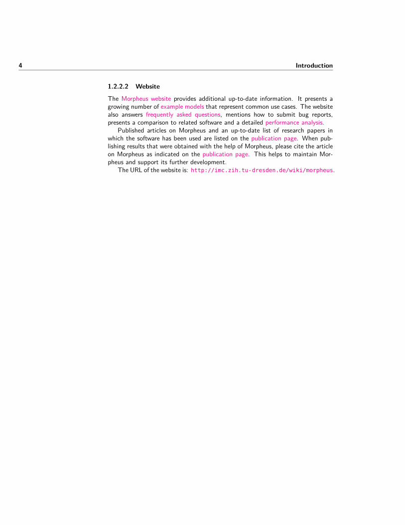
The GUI provides a series of editing tools that facilitate the construction andmodification of computational models and performs validation of the generatedXML models (see figure 2.1).

2.1.1

2.1.2

2.1.8 2.1.3

2.1.5

2.1.6

Figure 2.1: Editor view. This view is opened when selecting an element in the Documentspanel. Numbers correspond to sections in the text.

5

6 Graphical user interface

2.1.1 Examples

A number of example models is included in the application, accessible throughthe Examples menu in main toolbar. These examples demonstrate key featuresof Morpheus, show diverse use cases and modeling approaches and illustrate allelements of the Morpheus model description language.

These example models can serve as templates for the construction of newmodels. Detailed descriptions can be found on the website (fig. 5.1).

2.1.2 Documents panel

The Documents panel gives an overview of the opened documents and provides ameans to switch the current model. The main elements of each model are shownand can be edited via the context menu (right-click or ctrl-click). The contextmenu also allows the user to view the generated XML document.

2.1.3 Element editor

The Editor panel shows the editable tree-like structure of elements of the currentlyselected element in the Documents view. Elements can be added, copied or re-moved using the context menu. Adding an element opens a window showing a listof elements that can be added in the selected parent element. Required elementscannot be cut or removed, as to ensure model validity.

An element can also be temporarily disabled, which renders it ineffective withoutremoving it from the model. Disabled elements can afterwards be re-enabled.

2.1.4 Attribute editor

The Attribute panel shows a table of attributes of the element that is currentlyselected in the Editor panel. The first column shows attribute names and, for op-tional attributes, a checkbox. The second column allows users to specify parametervalues, depending on the type of attribute (double, integer, vector, string, etc.).Entries are validated by regular expressions. As long as an entry is invalid, it ismarked by a red background.

2.1.5 Expression editor

The Expression panel is a multiline editor to enter or edit the expression that iscurrently selected in the Editor panel. The editor enables users to specify math-ematical expressions as text in a familiar infix notation, using common operatorsand functions (listed in table 4.4). Expressions are formulated using predefined anduser-defined symbols (see table 4.1). For each model, the available symbols areshown in a list below the editor.

2.2. Simulation and results 7

2.1.6 Documentation

The Documentation panel provides a context-sensitive documentation of the ele-ment or attribute that is currently selected in the Editor or Attribute editor.

2.1.7 Clipboard

The Clipboard provides the ability to cut, copy and paste model elements. Becausethe clipboard is shared between documents, elements can be copied and pastedbetween models.

2.1.8 Fixboard

When loading documents with outdated or broken (yet well-formed) models, Mor-pheus attempts to repair the model by e.g. adding required elements or removingelements that are not allowed. The Fixboard provides a list of changes that havebeen made. Items in this list link to the element to which the changes have beenapplied.

2.2 Simulation and results

The GUI provides tools to execute (multiple) simulations called jobs, view simu-lation results, browse and restore jobs in the job archive and perform parametersweeps (see figure 2.2).

2.2.1 Simulation execution

Simulations are executed using the Start button in the simulation toolbar. Jobscan be executed in interactive, local and remote mode.

Interactive mode is the most verbose mode and useful for model testing. Graph-ical output generated by Gnuplot is displayed on screen (overriding the set-tings in analysis plugins). And error messages are displayed in a pop-up win-dow. The Stop button in the toolbar terminates the most recently startedrunning interactive simulation.

Local mode is the standard, non-verbose, execution mode for simulation on a lo-cal machine. Graphical output is stored in files. Error messages are displayedbelow the job queue. The Stop button in the toolbar is disabled.

Remote mode is th execution mode for large-scale simulation or batch processing.Jobs are executed on a remote high performance computing resource viassh, using the remote batch system (currently, only LSF is supported). SeeFile/Settings/Remote.

8 Graphical user interface

Figure 2.2: Results view. This view is opened at simulation start or upon selection a jobin the job archive (JobQueue). Numbers correspond to sections in the text.

2.2.2 Status and error messagesStatus and error messages of simulations executed in local mode are non-intrusivelydisplayed in the message box below the JobQueue panel. In interactive mode, theseerror messages are displayed in a pop-up window.

2.2.3 Job queue and archiveThe JobQueue panel provides an overview of pending, running, and completedsimulation jobs and shows the progress and execution time. Jobs can be stopped,removed and debugged (requires GNU debugger gdb) using the context menu.Jobs can be grouped and sorted according to model, job ID, state or sweep.

The result browser panel displays the content of the output folder of the cur-rently selected job. The toolbar allows jobs to be stopped (when running) andto open the output folder in a system-dependent file browser, or a command lineterminal.

2.2.4 Simulation output2.2.4.1 Visualization

Simulation data can be visualized in various ways. The method of visualization canbe configured in the Analysis element. Gnuplotter is the most versatile tool forvisualization of 2D simulations. It is based on the graphing utility Gnuplot. This

2.2. Simulation and results 9

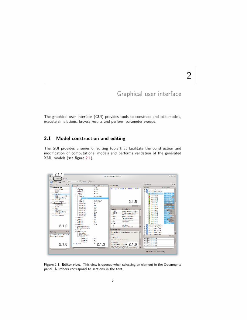
Table 2.1: Output files. Description of common output and result files.

File Descriptionmodel.xml XML model generated by GUI upon model execution.model.xml.out Standard output from simulator (as in Output panel).model.xml.err Error message generated by the simulator.[Title][Time].xml.gz Compressed XML model with simulation state, created if

and only if checkpointing enabled (Time/SaveInterval).logger_[Symbols].log ASCII text output from the Analysis/Logger plugin.cells_[Time].png

/jpg/gif/pdf

Plot generated by the Analysis/Gnuplotter plugin.

gnuplot_error.log Gnuplot error messages (if any).

analysis plugin can visualize both cells and PDE layers, provides customizable colorscales, and can display output to screen (wxt, aqua, x11, win) or write to file in anumber of image formats (png, jpg, pdf, svg).

For 3D simulations, the TIFFPlotter provides writing image stacks that maycontain 2D-5D data in the format [X, Y, Z, time, channel] that can be read byexternal image analysis software such as Fiji or ImageJ. Alternatively, 3D simulationdata can be written to VTK format using VTKPlotter for post-hoc visualizationwith ParaView.

The frequency of visualization is set by the interval attribute of the particularAnalysis element.

2.2.4.2 Logging and analysis

Simulation data can be exported to log files, either as raw data or in processed form.The Logger plugin writes cell property values or PDE values, optionally reducedafter summing or averaging. The SpaceTimeLogger provides a way to write valuesof a linear PDE layer or a slice of a 2D/3D PDE layer to construct space-timeplots. The HistogramLogger constructs and outputs frequency distributions ofcell properties in a population.

The result files are standard tab-delimited text files that can be imported andprocessed by external statistical software. Additionally, these logging tools includea Plot function to visualize the data.

The frequency of data output is set by the interval attribute of the particularAnalysis element.

2.2.4.3 Output folder

Simulation data is written to a folder [Title]_[JobID] within the simulation folderconfigured in Settings/Local. Before execution, the model XML file (i.e. model.xml)and dependent files (e.g. TIFF images) are written/copied to this folder. Duringexecution, simulation output is written to the same folder. The contents of theoutput folder can be browsed by selecting the job in the JobQueue panel. Table2.1 gives an overview of the files in the output folder.

10 Graphical user interface

Table 2.2: SBML import. Translation of SBML concepts (red) into Morpheus modeldescription language (blue).

SBML Morpheus MDL CommentSpecies Property Units are discardedParameter Property / Constant Depends on constant attributeInitialAssignment InitProperty

Functions Inlined in RateRule

AssignmentRule Equation

RateRule DiffEqn

AlgebraicRule not supported

Reaction Converted to RateRule

Event Event Delays are not supported

2.2.5 Restoring and checkpointingModels in the job archive can be restored by opening the file: model.xml. Thisopens the initial state of the simulation model as a new document.

When using checkpointing (Time/SaveInterval), the complete simulationstate is saved as a compressed XML file ([Title][Time].xml.gz) at the specifiedinterval. These files can be restored in the same way, however, in this case, a newdocument is opened containing the complete simulation state at time [Time].

2.2.6 SBML importMorpheus supports importing SBML models for intracellular dynamics. SBML(Systems Biology Markup Language) is a standard for describing models of bio-chemical pathways. SBML models can be generated using SBML simulators suchas Copasi or downloaded from public repositories such as the BioModels database.

Upon importing an SBML model, the SBML model is converted into systemsof ordinary differential equations for intracellular dynamics in Morpheus modeldescription language (MDL). Some SBML constructs can be translated in a one-to-one fashion into Morpheus MDL while others require a more elaborate conversion(see table 2.2).

In general, SBML models are imported in the following way (SBML constructsin red and Morpheus MDL constructs in blue):

1. A new non-spatial single-cell Morpheus model is created. This model specifiesa single lattice site and a population of 1 cell. A CellType is created tocontain the system of ordinary differential equations.

2. Matching concepts such as Species, Events, InitialAssignments, etc.are translated from SBML into the Morpheus MDL concepts of Property,Constants, Events, InitProperty, etc..

3. Reactions in the SBML model are, together with the associated KineticLawsand Functions, converted into SBML RateRules. These RateRules are

2.3. Parameter sweeps 11

subsequently assembled into a System of differential equations (DiffEqn)such that a single differential equation describes the temporal evolution of aSpecies or Parameter.

4. Unlike in SBML, the symbolic identifier of a Property or a Constant mustbe unique in Morpheus MDL. Therefore, if necessary, Reaction parametersare renamed upon import by appending the sequential reaction number.

5. Simulation details are not specified in SBML models but are required forsimulation. Therefore, default values are set during the import process. Sim-ulation time is assumed to run from 0...1 by setting Time/StartTime=”0”and Time/StopTime=”1”. The System solver is set to Runge-Kutta (RK4)by setting solver =”runge-kutta” and its time-step=”0.01”.

6. Finally, simulation output is preconfigured with a graphical visualization ofthe time course data of all species using Analysis/Logger/plot.

Note that not all SBML concepts can be converted into Morpheus MDL. In partic-ular, multiple compartments are not supported, and conversion of delay equationsis not possible (since Morpheus only supports delay differential equations with con-stant delays, see section 3.2.3). Furthermore, note that units and dimensions arediscarded upon import.

After importing an SBML model into Morpheus, it can be extended into aspatial, multicellular or multiscale model. Alternatively, it can be copied as amodule into an existing model using the Clipboard (see section 2.1.7).

2.3 Parameter sweeps

The GUI provides a convenient interface for batch processing by generating multiplejobs with different parameter sets. All parameters (Attributes and Expressions) canbe selected for parameter sweep, using the context menu item ParamSweep. Uponselection, the parameter appears in the ParamSweep view (fig. 2.3). This is openedwhen selecting the ParamSweep element in the Documents panel. This shows theXML path of the parameter and its type. The range of values for batch processingcan be set be editing the values in the third column. Values can be given explicitlyas semicolon-separated lists or using the list expansion syntax as shown in table2.3.

2.3.1 Multiple parametersBy default, parameter sets will be combined in a combinatorial fashion, such that ajob is created for each combination of parameter values. Note that the number ofsimulation jobs can get prohibitively large for multiple parameters. The number ofjobs is calculated for the current configuration and displayed above the parameters.

To have multiple parameters set simultaneously changing sets, a parametercan be dragged on another to couple them in a pairwise fashion. Note that theseparameter sets should be of the same length, otherwise, the lowest number ofparameter values is used for the paired set.

12 Graphical user interface

Figure 2.3: Parameter sweep view. This view is opened when selecting the ParamSweepelement in the Documents panel.

Table 2.3: Syntax for list expansion in parameter sweep view.

Syntax Examples ResultList x;x;x 1.0;1.5;3.0 1.0;1.5;3.0

10 10 10;20 20 20 10 10 10;20 20 20

square;hexagonal square;hexagonal

Range Increment x:x:x 0:2:10 0;2;6;8;10

0.5:1:3 0.5;1.5;2.5

Intervals x:#x:x 0:#2:10 0;5;10

0:#4:1.0 0;0.25;0.5;0.75;1.0

Logarithmic x:#xlog:x 1:#2log:100 1;10;100

2.3. Parameter sweeps 13

2.3.2 Simulation and resultsParameter sweeps are executed from the ParamSweep panel using the Start buttonin the toolbar. Note that the ParamSweep panel must be opened in order to starta parameter sweep. Upon execution, a folder [Name of Sweep] is created thatcontains a file sweep_summary.txt and subfolders for each simulation job. Thefile contains the folder names for the individual jobs and their parameter sets. andcan be used for post-hoc analysis.

2.3.3 Restoring parameter sweepsSettings of previous parameter sweeps can be restored from the JobQueue providedthat the selected model defined the same parameters and symbols.

3Model formalisms

Morpheus supports the simulation of discrete cellular Potts models as well as contin-uous ordinary differential equations (ODEs) and reaction-diffusion systems. Thesecore model formalisms are implemented in a modular way such that they can beflexibly integrated into multiscale models. Moreover, the modularity enables themto be combined into auxiliary formalisms such as finite state machines, cellularautomata, coupled ODE lattices or gradient-based models.

3.1 The System construct

The System is a mathematical construct in Morpheus MDL that plays a centralrole in modeling of temporal dynamics including ordinary differential equation,reaction-diffusion systems as well as rule-based models such as cellular automata.

A System is an environment for tightly coupled sets of (differential) equations.Rules or differential equations in a System environment are updated synchronouslysuch that the states of variables at time t are calculated on the basis of the stateof the variables at the previous time t − ∆t. Algebraic loops within or betweenrules or differential equations are allowed (only) within a System. Therefore, re-currence equations (Rule) or tightly coupled differential equations (DiffEqn) canbe modeled within this environment.

A System is associated with a numerical solver and a time-step (as explainedin section 3.2.1). The time-step sets the integration time step used by the solverand should be set by the user on the basis of performance (large time-step) andaccuracy (small time-step) considerations.

In addition, the System has an optional attribute time-scaling (default =1.0) which scales the time within a System relative to the global time. Thisautomatically scales the System time-step such that the numerical accuracy ispreserved. The time-scaling attribute provides a convenient way to scale thedynamics of sub-models to each other.

3.2 Differential equations

A number of numerical solvers are available for (a subset of) ordinary, stochas-tic, delay and partial differential equations to solve initial value problems (Cauchy

15

16 Model formalisms

Table 3.1: Numerical solvers for ordinary and stochastic differential equations.

Method Numerical schemeEuler yn+1 = yn + ∆tf(tn, yn)

Heun (midpoint) yn+1 = yn + 12∆tf(tn, yn) + f(tn+1, yn+1)

whereyn+1 = yn + ∆tf(tn, yn)

Runge-Kutta (RK4) yn+1 = yn + 16∆t(k1 + 2k2 + 2k3 + k4)

wherek1 = f(tn, yn),k2 = f(tn + 1

2∆t, yn + 1

2∆tk1),

k3 = f(tn + 12∆t, yn + 1

2∆tk2),

k4 = f(tn + ∆t, yn + ∆tk3)

Euler-Maruyama yn+1 = yn + ∆tf(tn, yn) +√

∆t∆Wn

Heun-Maruyama yn+1 = yn + 12∆tf(tn, yn)+

√12∆t∆Wn +f(tn+1, yn+1)

whereyn+1 = yn + ∆tf(tn, yn) +

√12∆t∆Wn

problems) of the form dydt = f(t, y(t)) together with the initial condition y(t0) = y0.

Differential equations (DiffEqn) must be specified inside a System element thatprovides an environment for synchronous updating of tightly coupled updated dif-ferential equations.

3.2.1 Finite difference solvers

Morpheus implements finite difference methods, Euler, Heun and Runge-Kutta (seetable 3.1). The method to be used for a set of differential equations is specified inSystem/solver. All solvers have a fixed time-step that must be specified by theuser in System/time-step.

Note that forward solver methods are not suitable for solving stiff systemsand may require small time-steps to guarantee stability and sufficient accuracy.All solvers use fixed time stepping; adaptive time stepping solvers are not yetimplemented.

3.2.2 Stochastic differential equations

For stochastic differential equations, the Euler-Maruyama or Heun-Maruyamamethod is used (see table 3.1). These methods scale the noise amplitude to thetime-step h that is used. Morpheus automatically switches to Maruyama solvers

3.3. Reaction-diffusion models 17

when a DiffEqn contains a normally distributed random number, i.e. rand_-norm([mean],[stdev]).

Note that other random number distributions, e.g. uniform or gamma distribu-tions, are not allowed in this context. Moreover, stochastic differential equationscannot be solved using the Runge-Kutta method.

3.2.3 Delay differential equationsMorpheus supports delay differential equations through the use of a property

with a delay, a DelayProperty. This property has an attribute delay that specifiesthe length of history, i.e. the lag between assignment of a value and the time atwhich it is returned.

Note that only constant time delays are supported. Further note that the delaymust be a multiple of the solver time-step*time-scaling. Also note that a delaysmaller than this time-step has no effect.

3.2.4 Initial conditionInitial conditions for cell-bound variables, i.e. Celltype/Property can be specifiedin various ways, depending on whether the initial condition should be specified in ahomogeneous or heterogeneous way or to set an initial conditions in a cell-specificfashion.

3.2.4.1 Homogeneous population

The value specified in Celltype/Property/value serves as an initial conditionfor the whole population of this Celltype. Therefore, this method defines a cellpopulation that is homogeneous with respect to this variable.

3.2.4.2 Heterogeneous population

A heterogeneous cell population in which initial conditions differ per cell may beconfigured using a mathematical expression in Population/InitProperty. Thisenables setting initial conditions according to cell ID (cell.id), cell position(cell.center.x) or using random distributions (e.g. rand_uni([min],[max])).

3.2.4.3 Cell-specific initial conditions

Initial conditions may be specified for each cell separately in Population/Cell/-PropertyData, and likewise for vector and delay properties. When using check-pointing, the state of each cell-bound variable is stored here.

3.3 Reaction-diffusion models

Solvers are available for initial boundary value problems on a one-, two- or three-dimensional domain of length L of the form ∂y

∂t = D ∂2y∂x2 + f(t, y(t)) with initial

18 Model formalisms

conditions y(t0, x) = y0(x) and a set of boundary conditions such as y(t, 0) =y(t, L) = 0. Reaction-diffusion systems are solved using the sequential operatorsplitting method in which the original problem is split into two subproblems (thereaction and diffusion steps) that are solved sequentially, both for the same time-step. For the reaction step, one of the finite difference methods is used, as describedabove (section 3.2).

3.3.1 DiffusionThe diffusion equation is solved using the central difference method. The diffu-sion coefficient D is specified for each species in the reaction-diffusion systemsin Layer/Diffusion (default: 0.0). The spatial discretization h is specified inSpace/Lattice/NodeLength (default: 1.0).

During initialization, the numerical time-step for the reaction step is adoptedby the diffusion problem. If necessary, the time-step is automatically adjusted inorder to satisfy the Courant–Friedrichs–Lewy (CFL) condition, 2dD∆t

h2 ≤ 1 whered = 1, 2, 3 is the number of dimensions.

3.3.2 Boundary conditionsBoundary conditions can be either periodic (default), constant (Dirichlet) ornoflux (Neumann). These are specified in Space/Lattice/BoundaryConditionsfor each boundary separately (x, -x, y, -y, z, -z). Note that the type of boundarycondition is shared for all spatial model components (although values may differ).

3.3.2.1 Constant boundary value

In case of constant boundaries, for each species in the reaction-diffusion system,a value for each boundary should be specified in PDE/Layer/BoundaryValue (de-fault: 0.0).

3.3.2.2 Irregular domains

To solve reaction-diffusion systems in irregular domains, as often required in image-based systems biology, a shaped domain may be loaded from a TIFF image inSpace/Lattice/Domain/Image. This TIFF must be in 8-bit format in which zeropixels are interpreted as background (outside domain), non-zero pixels are setas foreground (inside domain). Irregular domains can have constant or nofluxboundaries.

3.3.3 Initial conditionInitial conditions for each species in the reaction-diffusion system can be set us-

ing mathematical expressions in PDE/Layer/Initial/InitPDEExpression. Thisenables setting up random initial conditions or spatial gradients. By specifyingsymbols for space and lattice size using user-defined symbols (see table 4.1), het-erogenous initial conditions can be specified, independent of spatial discretization.

3.4. Cellular Potts model 19

Table 3.2: Cellular Potts model parameters and their location in the model descriptionlanguage.

Symbol Description Morpheus MDLMetropolis kinetics CPM/MetropolisKinetics

T Temperature temperature

Y Yield yield

N Neighborhood Neighborhood

Sampling / stepper algorithm stepper

Interaction energy CPM/Interaction

J Interface energy Contact

Shape constraints CellTypes/CellType

Vt Target volume VolumeConstraint/target

λV Strength of volume constraint VolumeConstraint/strength

Pt Target perimeter SurfaceConstraint/target

λP Strength of perimeter constraint SurfaceConstraint/strength

Non-Hamiltonian CellType/CellType

µ Chemotactic sensitivity Chemotaxis/strength

3.4 Cellular Potts model

The cellular Potts model (CPM) is a cell-based time-discrete method that repre-sents individual cell shapes as lattice domains and models cell motility in termsof energy minimization using modified Metropolis kinetics. Table 3.2 provides anoverview of how cellular Potts model parameters are encoded in Morpheus MDL.

3.4.1 Modified Metropolis kineticsA CPM defines cell shape and motility constraints in terms of energetical con-straints, described in a Hamiltonian. Motility arises from updating the latticeconfiguration according to energy minimization, based on a modified Metropoliskinetics, with the following steps.

First, a lattice site x (target site) is chosen at random with uniform distribution(see 3.4.2). Second, a lattice site x′ (trial site) is chosen from the neighborhoodNx, with uniform distribution (see 3.4.3). Then, the change in free energy ∆His calculated for the case if the state σ at the trial site x′ would be copied to thetarget site x. Finally, whether or not this transition is accepted depends on ∆Haccording to a Boltzmann probability:

P (σx′ → σx) =

{1 if ∆H + Y < 0

e−(∆H+Y )/T otherwise

Here, T (for ’temperature’) modulates the probability of unfavorable updatesto be accepted, and represents local protrusions/retractions of the cell membrane.The parameter Y (for ’yield’) accounts for dissipative effects and represents forexample cytoskeletal resistance to membrane fluctuations.

20 Model formalisms

Figure 3.1: Neighborhood Order. Neighborhood of a lattice site (with dot) numberedaccording to the minimum neighborhood order in which they are included, for square(left) and hexagonal (right) lattices.

The parameters for the modified Metropolis kinetics are specified in CPM/-MetropolisKinetics.

3.4.2 StepperIn the standard random stepper algorithm, the target site x is selected at random,while the trial site x′ is selected from its local neighborhood. In certain cases,this can be highly inefficient. In sparsely populated lattices, for instance, thereis a high likelihood of selecting sites with identical states that cannot change theconfiguration. Selecting such sites is therefore redundant.

To prevent such meaningless updates, Morpheus provides the edgelist step-per. This sampling algorithm tracks all lattice sites that can potentially lead to achange in configuration and selects the target site x from this list with uniform ran-dom distribution. This can yield major improvements in computational efficiencywithout affecting model results.

The stepper algorithm can be selected in CPM/MetropolisKinetics/stepper(default: edgelist).

3.4.3 NeighborhoodThe size of the Neighborhood N can be specified using either Distance or Order.The Distance specifies the maximum Euclidean distance within which lattice sitesare considered neighboring sites. The Order uses a labeling scheme to identifythe neighboring sites. These labels are integer values that alternate between axial(odd numbers) and radial (even numbers) neighborhoods as shown in figure 3.1.

3.4.4 Monte Carlo Step (MCS) and time scalingWithin the CPM, a Monte Carlo step (MCS) is often interpreted as a discrete unitof time. A single Monte Carlo step is defined as the number of random sampledupdates equal to the number of lattice sites. That is within one MCS, on average,each lattice site has been sampled for an update.

3.4. Cellular Potts model 21

The duration of a single MCS is scaled to the global simulation time as specifiedin CPM/MCSDuration (default: 1.0).

3.4.5 Cell shape, interaction and motility

3.4.5.1 Hamiltonian

Each cell occupies a set of lattice sites x with its cell index σ > 0, whereasσ = 0 refers to the medium. Changes in the spatial configuration of cells onthe lattice are governed by a Hamiltonian H that describes the free energy ofthe lattice configuration. In its simplest form, ignoring intercellular interactionenergies, H =

∑σ>0 λV (vσ − Vt)2 where vσ is the actual volume (i.e. number

of lattice sites) of cell σ and Vt is the target volume. Deviations from the targetvolume increase the free energy H according to the elasticity parameter λV .

Additionally, a constraint on the perimeter of the cell is often used, H =∑σ>0

[λV (vσ − Vt)2 + λP (pσ − Pt)2

], where pσ is the actual perimeter (i.e.

number of interfaces between lattice sites) of cell σ and Pt is the target perimeterwith λP representing the elasticity parameter. The targets and scalars are writtenhere as constants for simplicity, but can be cell-specific and time-dependent, i.e.Vt,σ(t), by linking them to cell-bound variables or functions.

Hamiltonian terms for CPMmodels that constrain cell shape (VolumeConstraint,ShapeConstraint, LengthConstraint) can be specified in CellTypes/CellType.

3.4.5.2 Interaction energies

The CPM has been originally developed to study the effects of differential adhesionon cell sorting. Adhesion can be modeled using interaction energies that define afree energy penalty per interface of contact between cells. Differential cell adhesioncan be modeled by specifying different interaction energies for contacts betweendifferent cells σ of different cell types τ . This extends the Hamiltonian with theterm H =

∑interfaces i,j J [τ(σi), τ(σj)] (1− δσiσj

) where J is a matrix of inter-action energies between different cell types τ(σi) and σi is the cell at lattice sitei. The Kronecker delta δσiσj = {1, σi = σj ; 0, σi 6= σj} ensures only interfacesbetween cells are taken into account.

The matrix of interaction energies between cell types can be specified in CPM/-Interaction. These energies are normalized by the number of neighbors suchthat the interaction energies are automatically rescaled when the lattice structureis changed.

Interaction energies can be altered based on the state of a cell property thatrepresents e.g. cadherin expression (AddonAdhesion) or on the combination ofproperties between neighboring cells to represent binding between heterophilic(HeterophilicAdhesion) or homophilic adhesion molecules (HomophilicAdhesion).These plugins can be specified in CPM/Interaction/Contact.

22 Model formalisms

3.4.5.3 Kinetic terms

The classical CPM has been extended by non-Hamiltonian terms. Since these termsdirectly affect the change in energy ∆H and may change the energy of the system,they are called kinetic terms. A widely used kinetic term biases motility of a cell σ inthe direction of a local concentration gradient of a species w in a reaction-diffusionmodel in order to represent chemotactic migration: ∆H =

∑σ>0 µ(wx′ − wx).

Kinetic terms that bias motility (Chemotaxis, Haptotaxis, DirectedMotion,Persistence) can be specified in CellTypes/CellType.

3.4.5.4 Event-based terms

Other CPM extensions are based on the cell state at the end of a Monte Carlo stepand are evaluated only once per Monte Carlo step, instead of every update trial.This includes extensions that model cell division (Proliferation) and cell death(Apoptosis). Proliferation triggers the division of a cell into two daughtercells, based on a condition. Apoptosis triggers the immediate removal of a cell(lysis) or setting its target volume to zero (shrinking) and removing the cellfrom the population only after it does not occupy any lattice sites.

3.4.5.5 Update-preventing terms

Some CPM extensions act to prevent updates altogether, based on some criterion.These include the Freezer that disables all updates for a particular cell, basedon a user-specified condition. It also includes the ConnectivityConstraint thatensures the cell is simply connected by preventing updates that would break thistopological constraint.

3.4.6 Initial condition of spatial configurationSimulations of cellular Potts models require the specification of at least one popula-tion of cells in CellPopulations/Population. By default, the specified numberof cells is distributed randomly in space using a uniform distribution, each celloccupying a single lattice site.

Spatially structured initial populations can be configured using InitRectangleand InitCircle. These initializers attempt to fit the specified number of cells ina regular fashion, with each cell occupying a single lattice site. Note that artefactsmay occur due to spatial discretization.

Initializing a population of cells with geometrical shapes can be configured usingthe CellObjects initializer. This allows for the specification of spheres, cylinders,boxes and ellipsoids that can be arranged along the orthogonal axes.

Cell populations can also be initialized from images using the TIFFReaderinitializer. This provides an interface to configure models from microscopy images.TIFF images may be in 8-, 16-, and 32-bit format and may contain multiple z-slices(image stacks). By convention, all pixels sharing a particular integer value will beadded to the same cell. The option keep_id ensures that this value is used as acell ID internally.

3.5. Auxiliary model formalisms 23

3.5 Auxiliary model formalisms

The modular design of the formalisms allows a number of auxiliary formalisms tobe constructed. For instance:

Coupled ODE Lattice Coupled ordinary differential equation lattice models canbe used to represent a regularly structured tissue in which each cell is repre-sented by an intracellular ODE model and communicates with its neighboringcells.Coupled ODE lattice models can be constructed by configuring a lattice ofcells, each occupying a single lattice site using InitRectangle. A CellTypewith a System of DiffEqn describing the intracellular dynamics. Intercellu-lar communication is modeled using a NeighborReporter that reports the(weighted) average of the properties of directly adjacent neighbor cells.

Cellular Automata (CA) Cellular automata are a widely used discrete-time, discrete-space, discrete-variable formalism to study the emergence of macroscopicbehavior from microscopic local rules.CA models can be constructed by configuring a lattice of cells, each occupy-ing a single lattice site using InitRectangle. A CellType with a Systemof synchronously updated Rules describes the state transitions, based on thestates of cells in the local neighborhood, reported using a NeighborReporter.

Gradient based models Gradient-based models can be used to describe pattern-ing of tissues under influence of a morphogen gradient, such as Wolpert’sclassical French flag model.Gradient-based models are built using a non-diffusive PDE Layer, initializedby a mathematical expression using an InitPDEExpression. A regular lat-tice of cells is configured by an InitRectangle, in which each cell measuresthe morphogen concentration at its location using a PDEReporter, based onwhich an Equation defines the cellular identity.

4Model description language

Morpheus simulation models are specified in a custom domain-specific model de-scription language (MDL). The XML-based language uses biological and math-ematical terminology to declaratively describe multiscale multicellular simulationmodels. It is composed of human-readable tags to represent the components ofbiological processes (table 4.2) and a number of mathematical constructs to definetheir dynamics and relations (table 4.3).

Morpheus simulation models are fully specified by single model descriptionfiles. These include the definition, configuration and and parameterization of(sub)models as well as the specification how these (sub)models are interlinked.Details on the numerical simulations are also stored in the model description filesuch as the simulation time, spatial discretization, initial conditions and the con-figuration of visualization and data output. For checkpointing, the complete stateof a simulation during execution can be stored in the same file format. The factthat the complete simulation model, including the description of its dynamics, isencapsulated in single files, render them suitable for archiving as well as modelexchange between users.

4.1 Declarative

The Morpheus model description language (MDL) separates modeling from imple-mentation by allowing the description of models in a declarative fashion. Modelsdescribe what processes are to be simulated rather than how this should be ac-complished. This distinguishes declarative languages such as the Morpheus MDLfrom imperative programming language such as C++ or Python that focus on thedescription of algorithmic control flow.

4.2 Domain-specific

The MDL uses a domain-specific markup language using vocabulary that is derivedfrom the application domain of multiscale and multicellular systems biology. Onthe one hand, it uses concepts such as cell types and populations, and biologicalprocesses such as proliferation and chemotaxis (table 4.2). On the other hand, itdefines a range of mathematical constructs such as constants, functions, equations

25

26 Model description language

and systems of differential equations (table 4.3). This combination of biologicaland mathematical terms provides a powerful way to describe the relations anddynamics of biological processes.

4.3 Encapsulation

Models in Morpheus MDL describe both the model itself and specify details ofits simulation including initial conditions (see table 4.2). During a simulation, thefull simulation state, including the position and state of all cells, can be writtenin the same description language. In this way, a single model file contains the fullspecification of the model simulation. The encapsulation in a single file significantlysimplifies archiving, checkpointing and restoring simulation models as well as theexchange of models between users.

4.4 Two-tiered architecture

Morpheus MDL has a two-tier architecture (see figure 4.1). On the one hand, theXML is used to store information about the model components or sub-models in ahierarchically structured way. On the other hand, symbolic interdependencies rep-resent the interactions and feedbacks between model components or sub-models.This combination provides a convenient way to express models of complex biolog-ical processes and allows automation of model integration (see chapter 5).

4.4.1 XMLThe model description language is based on the eXtensible Markup Language(XML). This has a number of advantages: It stores information in a well-structuredfashion that can be easily parsed and validated and it allows human-readabledomain-specific terminology and can be extended in a straightforward fashion.

The main elements of the XML structure, as shown in table 4.2, are used todescribe both the structure and parameterization of the model, and the details of itsnumerical simulation. The spatio-temporal aspects of the simulation are specifiedin the required Space and Time elements, the initial conditions or simulation stateare described in CellPopulations, data output and visualization is configured inAnalysis. The title and annotation of a model are added in the Descriptionelement.

The model itself is configured using the CellTypes, CPM, and PDE elements.The properties, behavior and dynamics of cells, including intracellular dynamics,are specified in the CellTypes element. The parameters of the cellular Potts modelare configured in the CPM element and the reaction-diffusion models are definedand configured in the PDE element. These elements are all optional such that thevarious model formalisms can be used in isolation as well as in combination.

The XML represents this information in a hierarchical tree-like structure thatreflects the structure of the modeled biological system. For instance, the main ele-ment CellPopulations can contain a Population that contains multiple Cells.

4.4. Two-tiered architecture 27

Figure 4.1: Schematic representation of the two-tier architecture. The hierarchical XMLtree provides information on the structure of the model and its components (coloredboxes). By defining and referring to symbolic identifiers, model components can be linkedtogether in a network (arrows). Systems (rounded grey boxes) provide an environmentfor tightly-coupled differential equations in which self-references and circular dependenciesbetween symbols are allowed.

Similarly, intracellular dynamics are modeled using a Systems of DiffEqn withina CellType, while the PDE describing extracellular dynamics is defined in its ownelement outside of CellTypes.

The XML structure is convenient to represent the hierarchy between the compo-nents of a model. However, it is not suitable to describe the network of interactionsand feedbacks between these components, which is done using symbolic identifiers.

4.4.2 Symbols

Model components can be linked using symbolic identifiers. Symbolic identifiersand references establish interactions and feedbacks between (sub)models to repre-sent the network-like complexity in biological processes (see fig. 4.1).

Symbolic identifiers, or symbols, can be specified to represent user-definedmodel variables such as cell-bound properties (Property) or concentrations ofspecies in a reaction-diffusion model (Layer) (see table 4.1). Symbols can also

28 Model description language

be specified for simulation-related constants and variables such as lattice size andcurrent time of simulation (see table 4.1). Symbols can be used in mathematicalexpressions to define relations between model components. Additionally, symbolsprovide a convenient way to integrate different (sub)models by defining symbolicidentifiers in one (sub)model and using them in another (sub)model.

4.5 Mathematical constructs

The model description language provides a number of mathematical constructsto define constants and variables and to express functions, equations and condi-tional events as well as the specification of tightly coupled systems of differentialequations. An overview of the available constructs is given in table 4.3.

Mathematical expressions may be specified in terms of user-defined or prede-fined symbols (see table 4.1). Expressions are entered in plain text using standardinfix notation. An overview of the available operators, functions and random num-ber generators and their syntax is given in table 4.4.

Expressions are parsed during initialization using the fast math parser muparser(muparser.beltoforion.de). Muparser converts expressions to reverse Polishnotation represented in byte code that is used to evaluate the mathematical ex-pressions at run time.

4.6 XML schema

The rules, constraints and contents of the Morpheus model description languageare laid down in an XML schema. The XML schema description (XSD) is em-bedded in the GUI and provides the information to edit, validate and repair modeldescriptions. Although the XML schema validates the XML structure, the GUIdoes not check the correctness of symbolic linking and mathematical expressions.Therefore, syntactically correct models may still result in simulation errors despitevalidation by XML schema.

4.6. XML schema 29

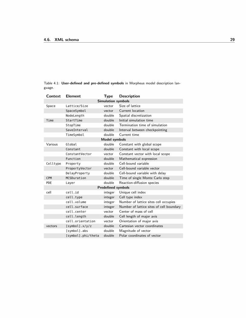
Table 4.1: User-defined and pre-defined symbols in Morpheus model description lan-guage.

Context Element Type DescriptionSimulation symbols

Space Lattice/Size vector Size of latticeSpaceSymbol vector Current locationNodeLength double Spatial discretization

Time StartTime double Initial simulation timeStopTime double Termination time of simulationSaveInterval double Interval between checkpointingTimeSymbol double Current time

Model symbolsVarious Global double Constant with global scope

Constant double Constant with local scopeConstantVector vector Constant vector with local scopeFunction double Mathematical expression

Celltype Property double Cell-bound variablePropertyVector vector Cell-bound variable vectorDelayProperty double Cell-bound variable with delay

CPM MCSDuration double Time of single Monte Carlo stepPDE Layer double Reaction-diffusion species

Predefined symbolscell cell.id integer Unique cell index

cell.type integer Cell type indexcell.volume integer Number of lattice sites cell occupiescell.surface integer Number of lattice sites of cell boundarycell.center vector Center of mass of cellcell.length double Cell length of major axiscell.orientation vector Orientation of major axis

vectors [symbol].x/y/z double Cartesian vector coordinates[symbol].abs double Magnitude of vector[symbol].phi/theta double Polar coordinates of vector

30 Model description language

Table 4.2: Model description language. A summary of the main elements of theMorpheus description language and their most important sub-elements. Required(sub)elements are printed in boldface.

Element Description Sub-elementsDescription Sets the name (Title) of the model, used for

naming the destination folder. May include modelannotation (Details), used for human-readableannotation only.

Title

Details

Space Sets the size, structure and boundary conditions ofthe lattice (Lattice). Optionally, sets a symbols forthe lattice size and current location(Lattice/Size/symbol and SpaceSymbol).

Lattice

SpaceSymbol

Time Set the duration of a simulation (StartTime andStopTime) defining the global time. Optionally, setsa symbol for current time (TimeSymbol). Mayspecify the interval to save the simulation state(SaveInterval). May set a random seed forstochastic simulations (RandomSeed).

StartTimeStopTimeTimeSymbolSaveInterval

RandomSeed

CellTypes

CellType

Allows multiple cell types to be defined. Each celltype (CellType) sets a name and type (i.e.biological or medium).May define multiple properties (Property) for use inmathematical expressions (Equation, ...). Maycontain reporters for spatial mapping (Reporter).May define systems of ordinary differential equations(ODE) (System/DiffEqn). May specify a diversity ofcellular behaviors (Chemotaxis, Proliferation, ...).

PropertySystemConstantFunctionEquationEventReporterChemotaxisProliferation

...

CPM Sets the time-scale of a Monte Carlo step(MCSDuration), the parameters for the cellular Pottsmodel (MetropolisKinetics) and the parameters ofinteractions between cells (Interaction).Optionally, for constant boundary condition, sets acell type at a boundary (BoundaryValue).

InteractionMetropolisKin.MCSDuration

BoundaryValue

PDE Sets the symbol and diffusion coeffients for species(Layer) in a reaction-diffusion model for use inmathematical expressions (Equation, ...). May set asystem of differential equations (System/DiffEqn)for reactions.

LayerConstantSystemFunction

Equation

CellPopulations

Population

Allows multiple populations to be defined. Eachpopulation sets a cell type and size (Population).May set initializers (e.g. Initrectangle). Mayexplicitly specify multiple cells with properties andpositions (Cell). When saving the simulation state,state of each cell is specified here.

CellInitrectangleTIFFReader

...

Analysis Sets the visualization and analysis tools. Maycontain various loggers and plotters (Gnuplotter,Logger). Executed at user-specified intervals.

GnuplotterTIFFPlotterLogger

HistogramLogger

4.6. XML schema 31

Table 4.3: Mathematical constructs. Overview of the mathematical constructs availablein model description language (• = symbol definition, ◦ = symbol reference).

Element Description Symbol graphContainers

Constant Constant value of type double with local scope, i.e. validwithin the CellType or System it is defined in. Constant

Global Variable value of type double with global scope.Global

PropertyPropertyVector

DelayProperty

Cell-bound variable. Property and DelayProperty are oftype double. DelayProperty has attribute delay to setthe lag between assignment and return of value.PropertyVector defines Euclidean vector in spacedelimited format “x y z”.

Property

Layer PDE model variable, i.e. species in reaction-diffusionsystem. Diffusivity of a Layer is specified in attributediffusion.

Layer

ExpressionsFunction Mathematical expression. Computes a value (double) for

the output symbol it defines, but does not assign it to avariable. Updated whenever when output symbol isreferenced. May not contain algebraic loop.

Function

Equation Mathematical expression. Computes a value (double) andassigns it to the variable it references. Updates arescheduled depending on its symbol dependencies. Maynot contain algebraic loop.

Equation

Rule Mathematical expression that defines a (recurrence)equation for use in environments such as System andEvent. Scheduled according to System/time-step. Maycontain algebraic loop and self-references.

Rule

DiffEqn Mathematical expression that defines a differentialequation. Only allowed in System environment. Maycontain algebraic loop and self-references.

DiffEqn

ReportersReporterNeighborsReporterPDEReporter

...

Explicit data mappings. Computes a statistic (average,mean, etc.) of the input data and assigns this to theoutput symbol. Updates are scheduled depending on itssymbol dependencies.

Reporter

EnvironmentsSystem Environment for tightly coupled sets of differential

equations and rules that are synchronously updated (seesection 3.1). Scheduled according to user-specifiedSystem time-step and time-scaling.

System

Event Environment for conditional or timed events. Triggeredperiodically or, if Condition is specified, whenever thecondition changes from false to true. Updates arescheduled according to time-step if specified ordepending on its symbol dependencies otherwise.

Event

32 Model description language

Table 4.4: Operators and predefined functions available in mathematical expressions.

Class Description SyntaxOperators Addition +

Subtraction -

Multiplication *Division /

Power ^

Logical operators Logical and and

Logical or or

Exclusive or xor

Comparison Equal ==

Not equal !=

Smaller < or &lt;

Greater > or &gt;

Smaller or equal <= or &lt;=

Greater or equal >= or &gt;=

Functions Sine sin(...)

Cosine cos(...)

Tangens tan(...)

Arc sine asin(...)

Arc cosine acos(...)

Arc tangens atan(...)

Hyperbolic sine sinh(...)

Hyperbolic cosine cosh(...)

Hyperbolic tangens tanh(...)

Arc hyperbolic sine asinh(...)

Arc hyperbolic cosine acosh(...)

Arc hyperbolic tangens atanh(...)

Logarithm base 2 log2(...)

Logarithm base 10 log(...)

Natural logarithm ln(...)

Exponent exp(...)

Power pow([base], [exponent])

Square root sqrt(...)

Sign, -1 if x<0, 1 if x>0 sign(...)

Round nearest integer rint(...)

Absolute abs(...)

Minimum of arguments min(..., ..., ...)

Maximum of arguments max(..., ..., ...)

Sum of arguments sum(..., ..., ...)

Average of arguments avg(..., ..., ...)

Modulus, remainder mod([numer], [denom])

Random number Uniform distribution rand_uni([min], [max])

Normal distribution rand_norm([mean], [stdev])

Gamma distribution rand_gamma([shape], [scale])

Boolean (0 or 1) rand_bool()

Condition Conditional statement if([condition], [then], [else])

5Model integration

Morpheus supports the integration of time-discrete cell-based models with time-continuous models for intra- and extracellular dynamics. In particular, cellular Pottsmodels (CPM) can be linked to ordinary, stochastic or delay differential equationsas well as to reaction-diffusion (PDE) models. The Morpheus model descriptionlanguage facilitates the specification of links between (sub)models with the help ofsymbolic identifiers (see chapter 4).

For the user, a link between sub-models is established by simply defining asymbol in one sub-model and using it as an input in another sub-model, providinga convenient way to construct and explore complex multiscale biological systemsusing integrative models. During simulation, Morpheus makes the data accessiblebetween sub-models and, if necessary, mapping or transforming it to make it suit-able for the target sub-model. Moreover, the updates of the various sub-models areappropriately scheduled, by determining the correct order and the frequency of up-dates, as to guarantee that up-to-date data is used in all computations. Both tasksare handled automatically as far as possible, based on user-specified time-steps andsymbolic interdependencies.

5.1 Spatial mapping

Integration of spatial model formalisms, i.e. cell-based and reaction-diffusion mod-els, requires that the data from one sub-model is accessible to the other sub-model.In Morpheus, data is not copied between sub-models, but is directly accessiblethrough symbolic identifiers. Yet, the data must be accessed in a way that isappropriate for the model that uses the symbol. The model that uses a symboldetermines the lattice sites for which the symbol is resolved, whereas the modelthat defined it determines the value of the symbol at those lattice sites.

Morpheus uses the convention that the spatial discretization in cell-based andreaction-diffusion models is identical. The lattice size (Lattice/Size) and thephysical interpretation of the size of a lattice site (Lattice/NodeLength) areshared by both CPM and PDE models, which simplifies their integration. There-fore, in some cases, the mapping is trivial enough to be handled automatically.In other cases, a more complex mapping is required such as calculating a sum oraverage which requires the explicit instructions by the user using a Reporter.

33

34 Model integration

5.1.1 Automated mapping

Mappings that present an unambiguous relationship are resolved automatically.For instance, when non-spatial constants and variables are used within a spatialcontext, the same value is used for all lattice sites over which is iterated. The useof symbols referring to cell-boundary Properties within reaction-diffusion (PDE)models linking PDE to CPM models can also be handled automatically. In that case,for each lattice site for which the PDE Layer is defined, the value of the cellproperty of the cell at that site is used.

The reverse case, when PDE variables are used in CPM models, can be automat-ically mapped, only in certain cases. For instance, in the Chemotaxis extension,cell motility is biased by the gradient of concentration of a species in a reaction-diffusion model. Here, the difference in concentrations of the PDE variable at thetarget and trial site is automatically resolved (see 3.4.5.3).

5.1.2 Explicit mapping with Reporters

When the mapping between the two contexts is not unambiguous, a statistic isrequired to define how a symbol should be mapped. This requires the user tospecify an appropriate way to transform the data from one (sub)model to theother (sub)model. Defining such an explicit mapping is done using a Reporter.

The NeighborsReporter calculates the (weighted) average or sum of the cell-bound Property in adjacent cells given by the input symbol and assigns thisstatistic to its output symbol.

The PDEReporter maps PDE variables for use in cell-based models by reportingthe average, sum, maximum or gradient of concentration of the input PDE/Layerat the lattice sites occupied by the cell or, optionally, its discretized center of mass.

5.2 Scheduling

Integration of time-continuous ODE and PDE models with time-discrete CPMmodels and various auxiliary mathematical constructs requires a careful schedul-ing of numerical updates. While the general simulation schedule is executed infixed order, some processes must be scheduled according to the symbolic inter-dependencies in order to guarantee correctness of simulation results. The simula-tion schedule is computed during intializatoin and printed to the standard output(model.xml.out).

5.2.1 Simulation schedule

The general simulation cycle follows a fixed order in which temporal models areexecuted before the sequential processes and output processes, as shown in figure5.1. The scheduling of sequential processes such as Reporters and Equationsinvolves the determination of the order of updates as well as the setting of intervalsin which the various model components should be computed.

5.2. Scheduling 35

Initialization Simulation cycle Termination

Systems Diffusion

CPM

Equations

Reporters

Events

Analysis

Save state

Lattices

Cell types

CPM

PDE

Cell populations

xSymbols

Reporters

Equations

Analysis

Save state

Analysis

Save state

1

2

3

StartTime

StopTime

Figure 5.1: Overview of the general simulation schedule. Between initialization andtermination, the simulation cycle is iteratively executed until time=StopTime. A singlesimulation cycle proceeds in three phases. First, the temporal models such as CPM ,Systems and Diffusion are updated according to user-defined time-steps. Second, thesequential processes such as Equations and Reporters are updated in an order andinterval that is determined by dependencies between symbols. Third, output is generatedand the simulation state is written to file at user-defined intervals.

Initialization

First, the lattice is created and initialized, cell types are created, the CPM is initial-ized, and PDE layers are created and initialized (PDEInitExpression). Afterwards,populations of cells are created and put in the lattice randomly or according to auser-specified initializer (e.g. InitRectangle). Then, symbols are registered andset to initial values. Afterwards, Reporters and Equations are run once to initializeall remaining symbols. Finally, the analysis and visualization tools (Analysis) arerun, and the simulation state is saved to file.

Simulation cycle

The simulation cycle is iterated from StartTime to StopTime in steps that advanceaccording to the smallest time step (section 5.2.3). In each iteration, the processesthat are scheduled for the current time step are executed in the following order.

1. Temporal models: The time-dependent models are executed. A singleMonte Carlo Step is performed for the CPM. Afterwards, Systems and Diffusionare updated.

36 Model integration

2. Sequential processes: Non-time-dependent models such as Equations,Reporters and Events are updated. Their order is computed from theirsymbolic interdependencies (section 5.2.2).

3. Analysis: Finally, visualization and data output is updated and the simula-tion state is saved to file.

Termination

At the end of simulation, visualization and analysis tools specified in Analysis toolscan be executed once more and the simulation state is written to file.

5.2.2 Scheduling update orderThe order of execution is independent of the order in which model componentsare specified in the model description file. Rather, updates of temporal processes(CPM, System, Diffusion) are scheduled according to the fixed schedule shown infigure 5.1 and updates of sequential processes such as Equations and Reportersare scheduled according to their symbolic interdependencies.

Sequential processes are ordered according to the dependencies in their inputand output symbol based on the following rule:

• Before updating a process, its input symbols must all be updated.

This is achieved by scheduling all processes that have these symbols as an outputbefore. Note that this is only possible if no algebraic loops or circular dependenciesexist between these processes. Therefore, such loops are only allowed within theSystem environment.

The order of execution of data output and visualization in Analysis is arbitraryand does not affect the simulation itself. Therefore, these are executed in the orderin which they are given in the model description file.

5.2.3 Update intervalThe simulation cycle is iterated for the period from StartTime to StopTime, calledthe global simulation time. The number of iterations that are executed during thisperiod depends on the temporal process with the smallest time step. During eachiteration, only the processes that require updating are executed. The intervals atwhich each process requires updating are determined during initialization, basedon user-specified time-steps or symbolic interdependencies.

The frequency in which CPM and Systems are updated is based on user-specifiedinformation. The update interval of CPM models is the duration of a single MonteCarlo step, specified in CPM/MCSDuration (see 3.4.4). The update interval ofa System is determined by its time-step, divided by time-scaling (see 3.1).Similarly, the intervals at which Analysis processes are executed to do visualizationand data analysis also depend on a user-specified interval.

5.2. Scheduling 37

The update intervals of other processes such as Equations, Reporters, Eventsand Diffusion are automatically determined by propagation of the intervals oftheir input and output symbols, according to the following rules:

• The process is updated as often as its output symbol(s) are used.

• The process is not updated more often than its input symbol(s) can change.

The former ensures that up-to-date data is used in all processes, while the latterimproves computational performance by preventing redundant computations. Notethat processes are not scheduled and computed if their output symbol(s) is (are)not used.

The interval of Diffusion is likewise determined by the interval of its outputsymbol, but it may iterate multiple times with smaller intervals as to satisfy theCFL stability criterion (see 3.3.1). Functions are not explicitly scheduled anddo not have an update interval. Instead, they are updated whenever their outputsymbol is used, but at most once per minimal time step. User-specified intervalsfor Analysis processes smaller than the minimal time step are ignored, since thestate of the simulation cannot change within this interval.

The final simulation schedule including the computed order of execution andupdate intervals is calculated at the end of initialization and printed to the standardoutput. This is written to the output file model.xml.out and is displayed in theoutput text box of results view in the GUI (see 2.2).

Table 5.1: Example models are available in the application and described on the website.