Morningstar Global Risk Model MethodologyIn essence, the model seeks to identify a small number of...

?

Morningstar Global Risk Model Methodology

Introduction

Risk is inherent to investing. Developing a prospective view of risk allows investors to make investment

decisions tailored to their individual risk preferences and ultimately increase the utility derived from their

investment portfolio. A risk model forecasts the distribution of future asset returns. This distribution

contains all the information needed to assess the riskiness of a portfolio. As the forecasted distribution

widens, that indicates more uncertainty about the future return potential of the portfolio. As tail

probabilities increase, that indicates the portfolio has higher risk of experiencing an extreme loss. With

this forecast, investors are empowered to evaluate the riskiness of assets or portfolios of assets.

In essence, the model seeks to identify a small number of independent, latent sources of return.

Movements in these sources drive the movement in a comparably small number of interpretable factors.

An example of a factor is the exposure to particular industry currencies – for instance how much does an

increase in the Euro/USD exchange rate drive an increase in the value of a stock? Movements in the

factors drive asset returns.

Several methodological choices must be made when building a risk model. Our choices were made

with the goal of creating a unique, interpretable, responsive, and predictive model. We began with the

following assumptions about asset returns which shaped our methodological choices.

× There are a small number of independent sources of market movement which drive the majority of

variation in asset returns

× Asset returns are not normally distributed

× The distribution of asset returns changes through time

These three concepts are well-recognized and non-controversial, although some or all of them are often

ignored for convenience by risk modelling practitioners.

Morningstar Research

17 May 2017

Content

1 Introduction

2 Model highlights

2 Universe Construction

3 Factor Selection

7 Factor Premia Estimation

8 Forecasting Factor Co-movement

10 Forecasting Idiosyncratic Movement

10 Aggregating Forecasts to Portfolios

14 Conclusion

15 References

Appendix A

16 Estimation Universe

Construction Rules

Appendix B

18 Factor Exposure Definitions

Style Factors

Sector Factors

Region Factors

Currency Factors

Appendix C

25 Forecasted Statistics Definitions

Appendix D

29 Independent Component Analysis

Appendix E

31 Generalized Autoregressive

Conditional Heteroskedastic Normal

Inverse Gaussian

©2016 Morningstar, Inc. All rights reserved. The information in this document is the property of Morningstar, Inc. Reproduction or transcription by any means, in whole or part, without the

prior written consent of Morningstar, Inc., is prohibited.

Morningstar Global Risk Model – Version 1.2 | 17 May 2017

Healthcare Observer | 17 May 2017

of 35

Page 2 of 35

Model highlights

Several features make the Morningstar Global Risk Model unique:

1. We use proprietary fundamental based factors which we believe are superior drivers of returns.

Morningstar’s research group provides forward-looking ratings on assets which have been successful

in predicting the future distribution of returns. Factors based on these ratings also tend to be

uncorrelated with traditional risk factors, making them a complementary addition to our risk factor

model. Likewise, we have distilled Morningstar’s proprietary database of mutual fund holdings into

factors which are also uncorrelated predictors of the future distribution of returns.

2. We forecast the full probability distribution of future returns with non-normal distributions.

Our risk model is agnostic to any particular risk metric a user wishes to use. Volatility, conditional

value at risk, downside deviation, interquartile range, skewness, kurtosis and many other measures

can be calculated directly from the probability distribution that is output from our model.

3. We accommodate a range of time horizons.

There is no need to guess whether a “short term” model or “long term” model matches your

investment horizon.

4. We make no assumption that co-movement of returns is exclusively linear.

The common practice of building and analyzing only a covariance matrix misses the fact that stocks

can experience tail events at the same time. Our model directly captures higher co-moments of

returns, enabling the construction of portfolios which can control tail risk.

Universe Construction

We define an estimation universe of investible companies with reliable data on which to build the

model. Stocks outside the estimation universe – generally illiquid stocks with small market

capitalizations – are relegated to the extended universe. We only use stocks in the estimation universe

to derive model parameters. This ensures the model parameters are not influenced by illiquid stocks with

unreliable data. Further we assume that the factors driving return in small illiquid stocks, like currency

and region, are the same factors which drive return for large stocks.

Exhibit 1 Estimation and Coverage Universe

(All stocks in Morningstar’s Equity Database)

Estimation Universe

Approximately 7,000 stocks

(Curated broad group of large liquid stocks)

Coverage Universe

Approximately 44,000 stocks

(Small illiquid stocks)

Source: Morningstar.

Authors

Patrick Caldon, PhD

Senior Quantitative Analyst

+61 2 9276 4473

[email protected]

Lee Davidson, CFA

Head of Quantitative Research

+1 312 244-7541

[email protected]

Xin Ling

Senior Quantitative Developer

+1 312 696-6191

[email protected]

Harry Tan, CFA

Senior Quantitative Developer

+1 312 384-3832

[email protected]

mailto:[email protected]








of 35

Page 3 of 35

We aim for a broad selection of companies across regions and sectors which are liquid enough to be

investable for most investors and are large enough to represent a large portion of the investable

universe. The filtering process below results in an estimation universe that is roughly 85% the size of the

global equity market capitalization. Appendix A details the exact rules we use to filter our estimation

universe.

All market returns and factor inputs are converted into a US dollar denomination when appropriate; in

particular all market returns are calculated in US dollars except as otherwise noted. The outputs of the

model measure risk with a US dollar numeraire.

Factor Selection

There are many ways to estimate the co-movement of asset returns. A naïve approach might be to

calculate a sample covariance matrix using historical returns. Unfortunately, this solution suffers from

the curse of dimensionality, i.e. the number of parameters in the covariance matrix is huge relative to the

number of historical return observations. As a result, the covariance matrix will be dominated by noise

and will poorly forecast future co-movement.

To remedy this problem we use a well understood approach to reduce the number of dimensions –

factor modeling. By finding common factors that drive asset returns, we no longer need to model each

asset individually. We can instead model a much smaller number of factors. This reduces the dimension

of our problem to reasonable levels and allows us to generate estimates of future co-movement.

There are several key notions needed to understand the way this model works:

× An asset return is the return of an investible security over a time period

× A factor is an observable data point that appears to influence asset returns, like Liquidity or Sector.

× A factor exposure is a number that measures how much an asset's return is influenced by a factor.

Exposures can be positive, negative or zero. Exposures change through time

× A factor premium is a number which represents how much a particular factor has influenced asset

returns for a particular time period

× We will later introduce sources. These are unobservable phenomena discovered through statistical

inference that drive some collection of factor premia.

We set out with several criteria when selecting factors for our model.

1. Our factors should have an economic basis and empirical relevance as predictors of the future

distribution of asset returns

2. Our factors should be interpretable and lend insight to a risk attribution analysis

3. Our factor set should be parsimonious

4. Our factor exposures should be practical to calculate





of 35

Page 4 of 35

Ultimately, we arrived at 36 factors which fall naturally into four distinct groups: style, sector, region and

currency. A short exposition on these factors is below. A more detailed treatment can be found in

Appendix B.

Style Factors

Our 11 style factors are normalized by subtracting the cross-sectional mean and then dividing by the

cross-sectional standard deviation, so a score of zero can always be interpreted as the average score,

and a non-zero score of n can be interpreted as being n standard deviations from the mean. In addition,

we modify the sign of our exposures so the premia associated with them are generally positive.

Exhibit 2 11 Style Factors

Name Description

Valuation The ratio of Morningstar’s quantitative fair value estimate for a company to its current market price.

Higher scores indicate cheaper stocks.

Valuation Uncertainty The level of uncertainty embedded in the quantitative fair value estimate for a company. Higher

scores imply greater uncertainty.

Economic Moat A quantitative measure of the strength and sustainability of a firm’s competitive advantages. Higher

scores imply stronger competitive advantages.

Financial Health A quantitative measure of the strength of a firm’s financial position. Higher scores imply stronger

financial health.

Ownership Risk A measure of the risk exhibited by the fund managers who own a company. Higher scores imply more

risk exhibited by owners of the stock.

Ownership Popularity A measure of recent accumulation of shares by fund managers. Higher scores indicate greater recent

accumulation by fund managers.

Liquidity Share turnover of a company. Higher scores imply more liquidity.

Size Market capitalization of a company. Higher scores imply smaller companies.

Value-Growth Value-Growth, where a value stock has a low price relative to its book value, earnings and yield.

Higher scores imply firms that are more growth and less value oriented.

Momentum Total return momentum over the horizon from -12 months through -2 months. Higher scores imply

greater return momentum.

Volatility Total return volatility as measured by largest minus smallest 1month returns in a trailing 12 month

horizon. Higher scores imply greater return volatility.






of 35

Page 5 of 35

Sector Factors

Our 11 sector factors measure the economic exposure of a company to the 11 Morningstar sectors. We

perform a Bayesian time-series regression analysis to find the exposures of an individual company to the

sector return with a prior based on the discrete sector classification of Morningstar’s data analysts. We

enforce constraints that our sector exposures, including the intercept term, must sum to 1 and must

individually be between 0 and 1.

× Basic Materials

× Energy

× Financial Services

× Consumer Defensive

× Consumer Cyclical

× Technology

× Industrials

× Healthcare

× Communication Services

× Real Estate

× Utilities

Region Factors

Our 7 region factors represent the economic exposure of a company to the 7 Morningstar regions. We

perform a Bayesian time-series regression analysis to find the exposures of an individual company to the

return of the portfolio of stocks in the region with a prior based on the discrete Region classification of

Morningstar’s data analysts.

× Developed Americas

× Developed Europe

× Developed Asia Pacific

× Emerging Americas

× Emerging Europe

× Emerging Asia Pacific

× Emerging Middle East





of 35

Page 6 of 35

Currency Factors

Our 7 currency factors represent the economic exposure of a company to 7 major currencies, excluding

US dollars. We perform a time-series regression analysis to find the exposures of an individual

company’s return denominated in US dollar currency to the following list of currency returns. We

calculate the return of these currencies against the US dollar.

× Euro

× Japanese Yen

× British Pound

× Swiss Franc

× Canadian Dollar

× Australian Dollar

× New Zealand Dollar

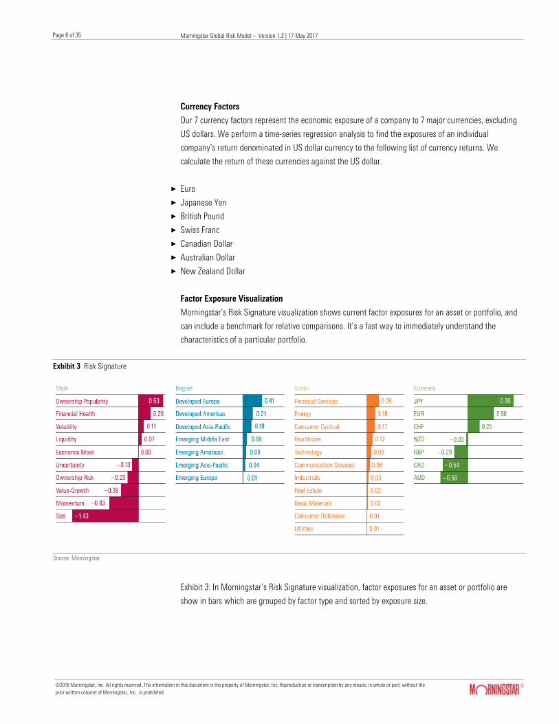
Factor Exposure Visualization

Morningstar’s Risk Signature visualization shows current factor exposures for an asset or portfolio, and

can include a benchmark for relative comparisons. It’s a fast way to immediately understand the

characteristics of a particular portfolio.

Exhibit 3 Risk Signature


Exhibit 3: In Morningstar’s Risk Signature visualization, factor exposures for an asset or portfolio are

show in bars which are grouped by factor type and sorted by exposure size.





of 35

Page 7 of 35

Factor Premia Estimation

Given a collection of factor exposures, Xt, for a set of n stocks at time, t, we perform a cross-sectional

regression of those exposures on total returns from t to t + 1, rt+1, to estimate the factor premia, ft.

𝑟𝑡+1 = 𝑋𝑡𝑓𝑡

+ 휀𝑡

Where: 𝑟𝑡 = (𝑛 × 1) 𝑣𝑒𝑐𝑡𝑜𝑟 𝑜𝑓 𝑠𝑡𝑜𝑐𝑘 𝑟𝑒𝑡𝑢𝑟𝑛𝑠 𝑎𝑡 𝑡𝑖𝑚𝑒 𝑡 𝑋𝑡 = (𝑛 × 𝑚) 𝑚𝑎𝑡𝑟𝑖𝑥 𝑜𝑓 𝑠𝑡𝑜𝑐𝑘 𝑒𝑥𝑝𝑜𝑠𝑢𝑟𝑒𝑠 𝑡𝑜 𝑓𝑎𝑐𝑡𝑜𝑟𝑠 𝑎𝑡 𝑡𝑖𝑚𝑒 𝑡; 𝑚 = 36 𝑓𝑡 = (𝑚 × 1) 𝑣𝑒𝑐𝑡𝑜𝑟 𝑜𝑓 𝑓𝑎𝑐𝑡𝑜𝑟 𝑝𝑟𝑒𝑚𝑖𝑎 𝑎𝑡 𝑡𝑖𝑚𝑒 𝑡 휀𝑡 = (𝑛 × 1) 𝑣𝑒𝑐𝑡𝑜𝑟 𝑜𝑓 𝑒𝑟𝑟𝑜𝑟 𝑡𝑒𝑟𝑚𝑠 𝑎𝑡 𝑡𝑖𝑚𝑒 𝑡

By repeating this cross-sectional regression, we construct an historical time series of the factor premia.

We use this time series of factor premia to analyze how each factor behaves in the context of the other

factors by examining factor co-movement in the history.

Exhibit 4 Historical Time Series of the Factor Premia


Exhibit 4: Morningstar’s Factor Premia visualization shows the cumulative return of our fundamental

style factor premia through time.

0

0.5

1

1.5

2

2.5

2003 2004 2005 2006 2007 2008 2009 2010 2011 2012 2013 2014 2015 2016 2017

Risk Factor Premia FAIRVALUE ECONOMICMOAT VALUATIONUNCERTAINTY

FINANCIALHEALTH VALUEGROWTH OWNERSHIPRISK

OWNERSHIPPOPULARITY SIZE LIQUIDITY





of 35

Page 8 of 35

Forecasting Factor Co-movement

Our co-movement forecasts are derived in a three-step process. We first perform a natural logarithm

transformation of our factor premia. We then remove the statistical dependency of the factors using a

technique known as Independent Component Analysis (ICA). Finally we forecast the statistically

independent sources using a time-series forecasting technique called a Generalized Autoregressive

Conditional Heteroskedastic Normal Inverse Gaussian GARCH-NIG distribution. This approach enables us

to forecast an entire non-normal distribution of returns for individual assets and portfolios.

Independent Component Analysis

ICA separates a collection of signal sources into their statistically independent driving factors. Our

factors share some mutual information which causes them to exhibit co-movement, and we need to

model this co-movement – or lack of statistical independence - if we are to estimate the future

distributions of portfolios.

ICA allows us to linearly transform our fundamental factors into latent “sources” which share minimal

mutual information. If sources share mutual information then analysis of some of the sources can deliver

useful information about other sources. This means in turn we cannot analyze the sources separately but

must analyze them jointly. This joint analysis is technically difficult. The practical significance of the ICA

transformation is that we no longer have to construct a joint distribution of the independent sources.

Instead we use univariate forecasting techniques, which we aggregate into forecasts for individual

assets and portfolios.

Specifically, ICA is a matrix factorization algorithm. It is used to decompose the matrix of demeaned

historical financial log-premia, F − F̅, into the product of a mixing matrix, A, and a matrix of a time series

of our statistically independent sources, S.

𝐹 − �̅� = 𝐴𝑆

Where: 𝐹 = (𝑚 × ℎ) 𝑚𝑎𝑡𝑟𝑖𝑥 𝑜𝑓 ℎ𝑖𝑠𝑡𝑜𝑟𝑖𝑐𝑎𝑙 𝑙𝑜𝑔 𝑓𝑎𝑐𝑡𝑜𝑟 𝑝𝑟𝑒𝑚𝑖𝑎 �̅� = (𝑚 × 1) 𝑣𝑒𝑐𝑡𝑜𝑟 𝑜𝑓 𝑢𝑛𝑐𝑜𝑛𝑑𝑖𝑡𝑖𝑜𝑛𝑎𝑙 𝑙𝑜𝑔 𝑓𝑎𝑐𝑡𝑜𝑟 𝑝𝑟𝑒𝑚𝑖𝑎 𝑚𝑒𝑎𝑛𝑠 𝐴 = (𝑚 × 𝑛) 𝑚𝑎𝑡𝑟𝑖𝑥 𝑜𝑓 𝑚𝑖𝑥𝑖𝑛𝑔 𝑐𝑜𝑒𝑓𝑓𝑖𝑐𝑖𝑒𝑛𝑡𝑠 𝑆 = (𝑛 × ℎ) 𝑚𝑎𝑡𝑟𝑖𝑥 𝑜𝑓ℎ𝑖𝑠𝑡𝑜𝑟𝑖𝑐𝑎𝑙 𝑠𝑡𝑎𝑡𝑖𝑠𝑡𝑖𝑐𝑎𝑙𝑙𝑦 𝑖𝑛𝑑𝑒𝑝𝑒𝑛𝑑𝑒𝑛𝑡 𝑠𝑢𝑏 − 𝑓𝑎𝑐𝑡𝑜𝑟𝑠

ICA is particularly well-suited for modeling financial returns or premia. ICA contrasts with principal

component analysis (PCA) by finding the statistically independent sources as opposed to the sources

which are merely uncorrelated. Given a sufficiently large quantity of normally distributed data, both PCA

and ICA should converge to identical decompositions up to negation and reordering of the rows of A.

But in the presence of non-normal data, ICA results in a more useful decomposition than PCA. It is

generally non-controversial that returns and risk premia are non-normally distributed, and we find this to

be true with our own premia data.





of 35

Page 9 of 35

There are several ways to characterize the estimation process for the mixing matrix, A, and the sources,

S. A straightforward way is to imagine that we have some method to measure the non-normality of a

sample of a weighted sum of the factors – we can do this by measuring the sample kurtosis, under the

assumption that a very high sample kurtosis means the weighted sum is non-normal. Suppose we can

somehow search the entire space of weights for the factors and find the weights which produce

maximal non-normality - call this a source. We then apply a mathematical operation to remove the

source we just discovered from the original collection of factors, and iterate the procedure on the factors

with this source removed. This operation produces the inverse matrix of A. A refinement and

formalization of these ideas is called “projection pursuit”. ICA has some technical differences to

projection pursuit but produces identical answers to under some formal conditions, most importantly

that the factors are produced by a weighted sum of independent non-normal sources. A more detailed

and technical description of the ICA methodology that we use in our risk model is found in Appendix D.

The Generalized Autoregressive Conditional Heteroskedastic Normal Inverse Gaussian (GARCH-

NIG) Model

We now need a model to forecast the distribution of our statistically independent sources. ICA relies on

the non-normality of the sources so a non-normal distribution seemed likely to be an appropriate model.

We examined several widely used non-normal univariate distributions to model the sources. The

distribution which struck the right balance of flexibility to model higher moments, mathematical and

computational tractability, and good model fit statistics was the Normal Inverse Gaussian (NIG)

Distribution.

The NIG distribution is a special case of the generalized hyperbolic distribution which has four

parameters, allowing it to flexibly model skewed and fat-tailed data. The density function is given below,

and straightforward expressions for the distribution’s mean, variance, skewness and kurtosis in terms of

these variables are in the appendix.

𝑔(𝑥; �̅�, 𝛽,̅ 𝜇, 𝛿) =�̅�

𝜋𝛿𝑒𝑥𝑝 (�̅� + �̅�

(𝑥 − 𝜇)

𝛿)

𝑲1 (�̅�√1 +(𝑥 − 𝜇)2

𝛿2 )

√1 +(𝑥 − 𝜇)2

𝛿2

Here 𝐊1 is the modified Bessel function of the third order and index 1. The four parameters

α̅ = δα, β̅ = δβ, μ, δ parameterize the distribution, where x, μ ∈ R, δ ≥ 0, 0 ≤ |β| ≤ α and γ̅ =

√α̅2 − β ̅2 . The expressions are written in terms of either α, β or α̅, β̅. The mean, variance and higher

moments of the distribution have straightforward expressions in these variables given in the appendix.

Still, fitting an NIG distribution as above to our data did not result in the desired dynamic properties of

our forecast. In particular the sources―like many asset returns―exhibit volatility clustering, so a large

movement in a source at time t tends to be followed by another large movement at time t + 1. The

effect is that we know the distribution parameters are changing over time, i.e. if the distribution has a

large dispersion at time t, then it will tend to have a large dispersion at time t + 1. We chose a





of 35

Page 10 of 35

methodology that generates a conditional forecast, i.e. a forecast that adapts to changing conditions to

capture phenomena such as volatility clustering. This is accomplished by fitting an NIG distribution with

zero mean and a variance of 1 to our historical normalized independent sources using maximum

likelihood estimation. We then multiply our NIG variable by a parameter, σt, which evolves as a

GARCH(1,1) process. This allows the variance of the distribution to change through time, while

preserving the tail and skewness characteristics.

Forecasting Idiosyncratic Movement

In addition to the factor premia, our cross-sectional regressions produce residual terms for each stock in

a particular time period which represent the portion of that stock’s return not explained by the

fundamental factors. In order to properly forecast the risk of the stock, we must also model this

idiosyncratic portion of returns.

We choose to model these log-transformed idiosyncratic returns exactly as we model our statistically

independent sources, using a GARCH-NIG model as described above. This allows us to have a time-

varying forecast which accommodates the fat tails and skewness which may be present in the

idiosyncratic returns.

Aggregating Forecasts to Portfolios

A portfolio’s return is the weighted average of the returns of its holdings. Using this fact we map the

return on a portfolio to a linear combination of independent components. We need not define a separate

set of equations for individual stocks because stocks can be thought of as a portfolio that is 100%

invested in a single holding.

A portfolio’s return pt is a weighted average of the returns of its holdings. pt = wtTrt

An asset’s return is an average of the returns of the factors weighted by the asset’s exposure to the

various factors plus the idiosyncratic return.

𝑟𝑡 = 𝑋𝑡𝑓𝑡 + 𝜖𝑡

A factor’s return is an exponential transformation of the average of the statistically independent source

returns weighted by its exposure to each source as determined by the mixing matrix.

𝑓𝑡

= 𝑒𝑥𝑝(𝐴𝑆𝑡 + �̅�) − 1 − �̅�

where 1 is a vector of ones. Therefore the portfolio’s return is an average of the independent source

returns weighted by the portfolio’s exposure to each source plus an average of the idiosyncratic returns

of its holdings weighted by the portfolio’s asset values.

𝑝𝑡 = 𝑤𝑡

𝑇(𝑋𝑡(𝑒𝑥𝑝(𝐴𝑆𝑡 + 𝑓̅) − 1) + 𝜖𝑡)

= 𝑤𝑡𝑇𝑋𝑡𝑒𝑥𝑝(𝐴𝑆𝑡 + 𝑓)̅ − 𝑤𝑡

𝑇𝑋𝑡1 + 𝑤𝑡𝑇𝜖𝑡





of 35

Page 11 of 35

Analytically Aggregating Moments

It is reasonable to assume investors derive utility from more than just the mean and variance of portfolio

returns. If we assume investors also care about skewness and kurtosis, then we must find the first four

raw moments of the portfolios forecast distribution. Mean, variance, skewness and kurtosis can all be

expressed as a function of a distribution’s raw moments as follows.

𝑀𝑒𝑎𝑛(𝑋) = 𝜇1 𝑉𝑎𝑟𝑖𝑎𝑛𝑐𝑒(𝑋) = 𝜇2 − 𝜇1

2

𝑆𝑘𝑒𝑤𝑛𝑒𝑠𝑠(𝑋) =𝜇3 − 3𝜇1𝜇2 + 3𝜇1

3 − 𝜇12

(𝜇2 − 𝜇12)1.5

𝐾𝑢𝑟𝑡𝑜𝑠𝑖𝑠(𝑋) =𝜇4 − 4𝜇1𝜇3 + 6𝜇1

2𝜇2 − 4𝜇13𝜇1 + 𝜇1

4

(𝜇2 − 𝜇12)2

Where:

𝜇𝑛

= 𝑡ℎ𝑒 𝑛𝑡ℎ 𝑟𝑎𝑤 𝑚𝑜𝑚𝑒𝑛𝑡 𝑜𝑓 𝑥 = 𝐸[𝑋𝑛]

We can find the raw moments of the portfolio from our equation above. Each of the terms below can be

expressed as a function of the moments of the NIG distribution for S_t and ϵ_t.

𝜇1 = 𝐸[𝑝𝑡] = 𝐸[𝑤𝑡

𝑇𝑋𝑡𝑒𝑥𝑝(𝐴𝑆𝑡 + 𝑓̅) − 𝑤𝑡𝑇𝑋𝑡1 + 𝑤𝑡

𝑇𝜖𝑡]

𝜇2 = 𝐸[𝑝𝑡2] = 𝐸 [(𝑤𝑡

𝑇𝑋𝑡𝑒𝑥𝑝(𝐴𝑆𝑡 + 𝑓)̅ − 𝑤𝑡𝑇𝑋𝑡1 + 𝑤𝑡

𝑇𝜖𝑡)2

]

𝜇3 = 𝐸[𝑝𝑡3] = 𝐸 [(𝑤𝑡


𝑇𝜖𝑡)3

]

𝜇4 = 𝐸[𝑝𝑡4] = 𝐸 [(𝑤𝑡


𝑇𝜖𝑡)4

]

We can find the nth raw moment or exponential transformed moments of any NIG distributed random

variable from its moment generating function. We replace the z with the moment order to get the

exponential transformed moments.

𝑀𝐺𝐹𝑥(𝑧) = 𝑒𝜇𝑧+𝛿(√𝛼2−𝛽2−√𝛼2−(𝛽+𝑧)2)

𝑥~𝑁𝐼𝐺(𝜇, 𝛼, 𝛽, 𝛿)

We produce multi-horizon forecasts over time periods longer than days by composing the returns over

several time periods.





of 35

Page 12 of 35

Approximating the Conditional Forecast Distribution

It can be useful to produce visualizations of the forecast distribution. To produce the forecast distribution

chart shown below, we need to draw the density function of a portfolio’s forecast returns at a given time

horizon.

We’ve shown that a portfolio can be modeled as a linear combination of the exponentially transformed

statistically independent sources of returns. Sometimes it is simpler to find the distribution with

parameters estimated using the method of moments to match the moments that are analytically derived

in the sections above.

First note that the characteristic function of a sum of independent random variables is equal to the

product of the characteristic functions of each variable. The characteristic function of an NIG distribution

follows.

φ(z) = e−iμz+δ(γ−√α2−(β+iz)2)

The characteristic function of the sum of variables is as follows.

𝜑𝑝(𝑣) = ∏ 𝜑𝑧𝑗,𝑡(𝑣)

𝐿+𝑁

𝑗=1

Finally, we can take the inverse Fourier transform of this characteristic function to arrive at the density

function for our portfolio.

𝑓𝑝(𝑟) =1

2𝜋∫ 𝑒−𝑖𝑣𝑟𝜑𝑝(𝑣)𝑑𝑣





of 35

Page 13 of 35

Exhibit 5 Morningstar’s Risk Forecast


Exhibit 5: Morningstar’s Risk Forecast visualization displays the full probability distribution of a stock or

fund relative to its most relevant benchmark along with summary statistics for a given time horizon. Data

is hypothetical for illustration purposes.





of 35

Page 14 of 35

Conclusion

The ability to model the risk of a portfolio is paramount to making investment decisions that maximize

utility. Our fundamental factor-based methodology provides a way to forecast risk, but more importantly,

it provides an intuitive interpretation of the mechanics behind the forecast. Monitoring factor exposures

and making economically sound decisions about which exposures are prudent and which are worth

avoiding is much easier when factor exposures are interpretable.

Our risk model includes factors unique to Morningstar. These factors which spring from our analyst-

driven research and our institutional portfolio holdings database are uncorrelated with more traditional

factors and helpful tools for an investor to use when tailoring their portfolio to suit their risk preferences.

Finally, we chose a non-traditional approach to modeling the future returns of our fundamental factors

through the use of Independent Component Analysis and a Generalized Autoregressive Conditional

Heteroskedastic Normal Inverse Gaussian process. This two-step procedure allows us to model the entire

non-normal joint distribution of future returns. From this joint distribution, we can calculate virtually any

risk statistic.

No risk model is perfect. Our aim has been to emphasize interpretability, responsiveness, and predictive

accuracy, and in doing so, we believe we’ve developed a unique model. We are grateful to the risk

modelers that paved the way for the methodological choices we’ve made along the way.





of 35

Page 15 of 35

References

Chen, Ying, Wolfgang Härdle, and Vladimir Spokoiny. "Portfolio value at risk based on independent

component analysis." Journal of Computational and Applied Mathematics 205.1 (2007): 594-607.

Chen, Ying, Wolfgang Härdle, and Vladimir Spokoiny. "GHICA—Risk analysis with GH distributions and

independent components." Journal of Empirical Finance 17.2 (2010): 255-269.

Chin, Elion, Andreas S. Weigend, and Heinz Zimmermann. "Computing portfolio risk using gaussian

mixtures and independent component analysis."Computational Intelligence for Financial Engineering,

1999.(CIFEr) Proceedings of the IEEE/IAFE 1999 Conference on. IEEE, 1999.

Cover, Thomas M., and Joy A. Thomas. Elements of information theory. John Wiley & Sons, 2012.

Ghalanos, Alexios, Eduardo Rossi, and Giovanni Urga. "Independent factor autoregressive conditional

density model." Econometric Reviews 34.5 (2015): 594-616.

Hyvärinen, Aapo, Juha Karhunen, and Erkki Oja. Independent component analysis. Vol. 46. John Wiley &

Sons, 2004.

Jensen, Morten B., and Asger Lunde. "The NIG‐S&ARCH model: A fat‐tailed, stochastic, and

autoregressive conditional heteroskedastic volatility model."The Econometrics Journal 4.2 (2001):

319-342.

Madan, Dilip B., and Ju-Yi J. Yen. "Asset allocation with multivariate non-gaussian returns." Handbooks

in Operations Research and Management Science 15 (2007): 949-969.

Morningstar Quantitative Equity Ratings Methodology. 2012.

<http://corporate.morningstar.com/US/documents/MethodologyDocuments/FactSheets/QuantitativeEq

uityCreditRatingsMeth.pdf>

Shephard, Neil G. "From characteristic function to distribution function: a simple framework for the

theory." Econometric Theory 7.04 (1991): 519-529.





of 35

Page 16 of 35

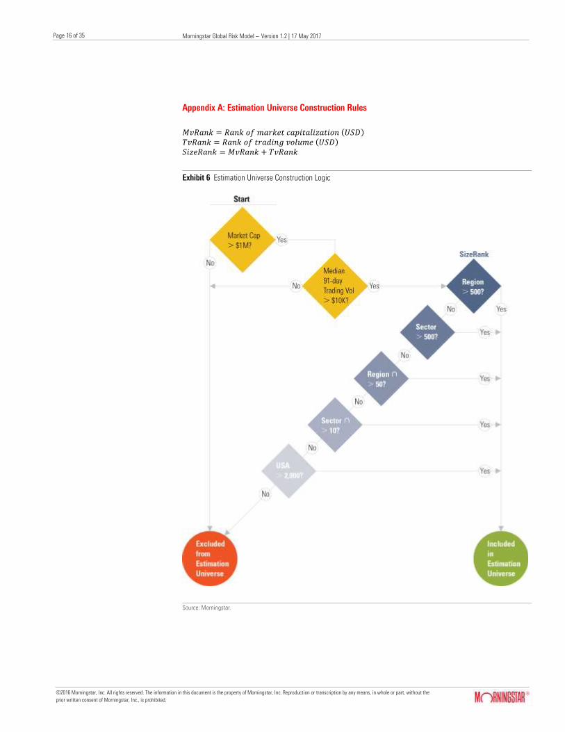
Appendix A: Estimation Universe Construction Rules

𝑀𝑣𝑅𝑎𝑛𝑘 = 𝑅𝑎𝑛𝑘 𝑜𝑓 𝑚𝑎𝑟𝑘𝑒𝑡 𝑐𝑎𝑝𝑖𝑡𝑎𝑙𝑖𝑧𝑎𝑡𝑖𝑜𝑛 (𝑈𝑆𝐷) 𝑇𝑣𝑅𝑎𝑛𝑘 = 𝑅𝑎𝑛𝑘 𝑜𝑓 𝑡𝑟𝑎𝑑𝑖𝑛𝑔 𝑣𝑜𝑙𝑢𝑚𝑒 (𝑈𝑆𝐷) 𝑆𝑖𝑧𝑒𝑅𝑎𝑛𝑘 = 𝑀𝑣𝑅𝑎𝑛𝑘 + 𝑇𝑣𝑅𝑎𝑛𝑘

Exhibit 6 Estimation Universe Construction Logic






of 35

Page 17 of 35

Appendix B: Factor Exposure Definitions

Style Factors

Valuation

The Valuation factor is the normalized ratio of Morningstar’s Quantitative Fair Value Estimate to the

current market price of a security. It represents how cheap or expensive a stock is relative to its fair

value. We arrive at a Quantitative Fair Value Estimate using an algorithm that extrapolates from the

roughly 1400 valuations our equity analyst staff assigns to stocks to a coverage universe of more than

45,000 stocks. For a detailed explanation of this methodology, please refer to the Morningstar

Quantitative Equity Ratings methodology document cited in the References section.

The Valuation factor is unbounded, and higher scores indicate cheaper stocks. A score of zero indicates

an average valuation.

Valuation Uncertainty

The Valuation Uncertainty factor is the normalized value of Morningstar’s Quantitative Valuation

Uncertainty Score. It represents the standard error of Morningstar’s Quantitative Valuation, in other

words, how unsure we are of a particular valuation. For a detailed explanation of this methodology,

please refer to the Morningstar Quantitative Equity Ratings methodology document cited in the

References section.

The Valuation Uncertainty factor is unbounded, and higher scores indicated more uncertain valuations.

A score of zero indicates an average level of uncertainty.

Economic Moat

The Economic Moat factor is the normalized value of Morningstar’s Quantitative Moat Score. It

represents the strength and sustainability of a firm’s competitive advantages. We arrive at a

Quantitative Moat Score using an algorithm that extrapolates from the roughly 1400 Economic Moat

ratings our equity analyst staff assigns to stocks to a coverage universe of more than 45,000 stocks.

For a detailed explanation of this methodology, please refer to the Morningstar Quantitative Equity

Ratings methodology document cited in the References section.

The Economic Moat factor is unbounded, and higher scores indicate stronger and more sustainable

competitive advantages. A score of zero indicates an average level of competitive advantages.





of 35

Page 18 of 35

Financial Health

The Financial Health factor is the normalized value of Morningstar’s Quantitative Financial Health Score.

It represents the strength of a firm’s financial position. The Quantitative Financial Health Score is driven

by market inputs, making it responsive to new information. It is calculated as follows.

𝑄𝐹𝐻 = 1 −(𝐸𝑄𝑉𝑂𝐿𝑃 + 𝐸𝑉𝑀𝑉𝑃 + 𝐸𝑄𝑉𝑂𝐿𝑃 × 𝐸𝑉𝑀𝑉𝑃)

3

Where: 𝐸𝑄𝑉𝑂𝐿𝑃 = 𝑝𝑒𝑟𝑐𝑒𝑛𝑡𝑖𝑙𝑒 𝑟𝑎𝑛𝑘 𝑡𝑟𝑎𝑖𝑙𝑖𝑛𝑔 300 𝑑𝑎𝑦 𝑒𝑞𝑢𝑖𝑡𝑦 𝑟𝑒𝑡𝑢𝑟𝑛 𝑣𝑜𝑙𝑎𝑡𝑖𝑙𝑖𝑡𝑦

𝐸𝑉𝑀𝑉𝑃 = 𝑝𝑒𝑟𝑐𝑒𝑛𝑡𝑖𝑙𝑒 𝑟𝑎𝑛𝑘 𝑜𝑓 𝐸𝑛𝑡𝑒𝑟𝑝𝑟𝑖𝑠𝑒 𝑉𝑎𝑙𝑢𝑒

𝑀𝑎𝑟𝑘𝑒𝑡 𝐶𝑎𝑝𝑖𝑡𝑎𝑙𝑖𝑧𝑎𝑡𝑖𝑜𝑛

The Financial Health factor is unbounded, and higher scores indicate stronger financial health. A score

of zero indicates an average level of financial health.

Ownership Risk

The Ownership Risk factor represents, for a particular stock, the ownership preferences of fund

managers with different levels of risk exposure. The Ownership Risk factor relies on current portfolio

holdings information and the raw Morningstar 36-month Risk score. High Ownership Risk scores signify

that those stocks are currently owned and preferred by fund managers with high levels of Morningstar

Risk. If high-risk managers are purchasing these stocks, then those stocks are likely to be high-risk. A

stock’s characteristic is therefore defined by who owns it.

The Ownership Risk score is calculated in the following manner:

𝑂𝑤𝑛𝑒𝑟𝑠ℎ𝑖𝑝 𝑅𝑖𝑠𝑘𝑛

= ∑ 𝑣𝑚,𝑛𝑀𝑅𝐼𝑆𝐾36𝑚

𝑀

𝑚=1

Where:

𝑣𝑚,𝑛 =𝑤𝑚,𝑛

∑ 𝑤𝑚,𝑛𝑀𝑚=1

𝑀𝑅𝐼𝑆𝐾36 = 𝑀𝑜𝑟𝑛𝑖𝑛𝑔𝑠𝑡𝑎𝑟 𝑅𝑖𝑠𝑘 𝑆𝑐𝑜𝑟𝑒 36 − 𝑚𝑜𝑛𝑡ℎ

In words, the Ownership Risk score for stock n is the weighted average of each manager m’s

Morningstar Risk 36-month score multiplied by the relative weight he/she holds in stock. After raw

scores are calculated, Ownership Risk scores are cross-sectionally normalized.

The Ownership Risk score is unbounded, and higher scores indicated stronger ownership preference for

risk. A score of zero indicates an average level of ownership preference for risk.





of 35

Page 19 of 35

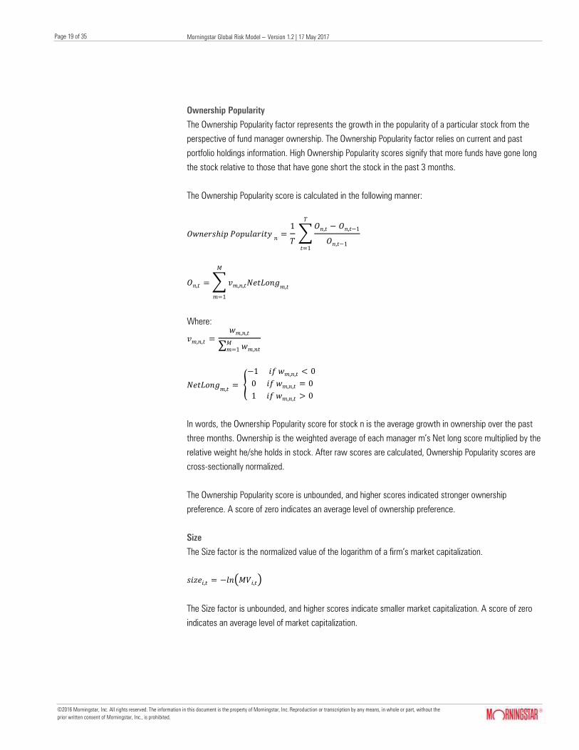
Ownership Popularity

The Ownership Popularity factor represents the growth in the popularity of a particular stock from the

perspective of fund manager ownership. The Ownership Popularity factor relies on current and past

portfolio holdings information. High Ownership Popularity scores signify that more funds have gone long

the stock relative to those that have gone short the stock in the past 3 months.

The Ownership Popularity score is calculated in the following manner:

𝑂𝑤𝑛𝑒𝑟𝑠ℎ𝑖𝑝 𝑃𝑜𝑝𝑢𝑙𝑎𝑟𝑖𝑡𝑦 𝑛

=1

𝑇 ∑

𝑂𝑛,𝑡 − 𝑂𝑛,𝑡−1

𝑂𝑛,𝑡−1

𝑇

𝑡=1

𝑂𝑛,𝑡 = ∑ 𝑣𝑚,𝑛,𝑡𝑁𝑒𝑡𝐿𝑜𝑛𝑔𝑚,𝑡

𝑀

𝑚=1

Where:

𝑣𝑚,𝑛,𝑡 =𝑤𝑚,𝑛,𝑡

∑ 𝑤𝑚,𝑛𝑡𝑀𝑚=1

𝑁𝑒𝑡𝐿𝑜𝑛𝑔𝑚,𝑡

= {

−1 𝑖𝑓 𝑤𝑚,𝑛,𝑡 < 0

0 𝑖𝑓 𝑤𝑚,𝑛,𝑡 = 0

1 𝑖𝑓 𝑤𝑚,𝑛,𝑡 > 0

In words, the Ownership Popularity score for stock n is the average growth in ownership over the past

three months. Ownership is the weighted average of each manager m’s Net long score multiplied by the

relative weight he/she holds in stock. After raw scores are calculated, Ownership Popularity scores are

cross-sectionally normalized.

The Ownership Popularity score is unbounded, and higher scores indicated stronger ownership

preference. A score of zero indicates an average level of ownership preference.

Size

The Size factor is the normalized value of the logarithm of a firm’s market capitalization.

𝑠𝑖𝑧𝑒𝑖,𝑡 = −𝑙𝑛(𝑀𝑉𝑖,𝑡)

The Size factor is unbounded, and higher scores indicate smaller market capitalization. A score of zero

indicates an average level of market capitalization.





of 35

Page 20 of 35

Liquidity

The Liquidity factor is the normalized value of the stock’s raw share turnover. The raw share turnover

score is calculated as the logarithm of the average trading volume divided by shares outstanding over

the past 30 days. It is essentially a churn-rate for a stock and represents how frequently a stock’s shares

get traded.

𝑠ℎ𝑎𝑟𝑒𝑡𝑢𝑟𝑛𝑜𝑣𝑒𝑟𝑖,𝑡 = 𝑙𝑛 (1

𝑇∑

𝑉𝑖,𝑡

𝑆𝑂𝑖,𝑡

𝑇

𝑡=1

) , 𝑤ℎ𝑒𝑟𝑒 𝑇 = 30

The Share Turnover factor is unbounded, and higher scores indicate higher liquidity. A score of zero

indicates an average level of liquidity.

Value-Growth

It is a reflection of the aggregate expectations of market participants for the future growth and required

rate of return for a stock. We infer these expectations from the relation between current market prices

and future growth and cost of capital expectations under the assumption of rational market participants

and a simple model of stock value. The Value-Growth factor is unbounded, and higher scores indicated

higher growth expectations and less value exposure. A score of zero is average.

Momentum

The Momentum factor is the normalized value of the stock price’s raw momentum score. The raw

Momentum score is calculated as the cumulative return of a stock from 365 calendar days ago to 30

days ago. This is the classical 12-1 momentum formulation except using daily return data as opposed to

monthly. To compute, US dollar currency returns are used.

𝑚𝑜𝑚𝑒𝑛𝑡𝑢𝑚𝑖,𝑡 = ∑ (𝑙𝑛 (1 + 𝑟𝑖,𝑡) − 𝑙𝑛 (1 + 𝑟𝑓𝑡))

𝑡−30

𝑡−365

The Momentum factor is unbounded, and higher scores indicate higher returns over the past year as well

as a propensity for higher returns in the future. A score of zero indicates an average level of momentum.

Volatility

The volatility factor is the normalized range of annual cumulative returns over the past year. Each day,

we compute the trailing 12-month cumulative return. Then, we look over the past year and identify the

maximum and minimum 12-month cumulative returns. We compute the range by taking the maximum

minus the minimum 12-month cumulative returns.

𝑟𝑎𝑛𝑔𝑒𝑖 = (𝑙𝑛 (1 + 𝑟𝑖,𝑡) − 𝑙𝑛 (1 + 𝑟𝑓𝑡))𝑚𝑎𝑥

− (𝑙𝑛 (1 + 𝑟𝑖,𝑡) − 𝑙𝑛 (1 + 𝑟𝑓𝑡))𝑚𝑖𝑛

The Volatility factor is unbounded, and higher scores indicate higher volatility. A score of zero indicates

an average level of volatility.





of 35

Page 21 of 35

Sector Factors

Sector exposures are calculated based on a time-series regression of excess stock returns to a set of

sector benchmarks.

𝑟𝑡𝑖 − 𝑟𝑡

𝑓 = 𝛼𝑖 + 𝛽1𝑖

(𝑟𝑡1 − 𝑟𝑡

𝑓) + ⋯ + 𝛽𝑘

𝑖(𝑟𝑡

𝑘 − 𝑟𝑡𝑓

) + 휀𝑡𝑖

𝑟𝑡𝑖 = 𝑤𝑒𝑒𝑘𝑙𝑦 𝑟𝑒𝑡𝑢𝑟𝑛 𝑜𝑛 𝑡ℎ𝑒 𝑖𝑡ℎ 𝑠𝑡𝑜𝑐𝑘

𝑟𝑡𝑓

= 𝑤𝑒𝑒𝑘𝑙𝑦 𝑟𝑒𝑡𝑢𝑟𝑛 𝑜𝑛 3 − 𝑚𝑜 𝑈𝑆 𝑇𝐵𝑖𝑙𝑙 𝑟𝑡

𝑘 = 𝑤𝑒𝑒𝑘𝑙𝑦 𝑟𝑒𝑡𝑢𝑟𝑛 𝑜𝑛 𝑡ℎ𝑒 𝑘𝑡ℎ 𝑠𝑒𝑐𝑡𝑜𝑟 𝑏𝑒𝑛𝑐ℎ𝑚𝑎𝑟𝑘 (𝑒. 𝑔. 𝐵𝑎𝑠𝑖𝑐 𝑀𝑎𝑡𝑒𝑟𝑖𝑎𝑙𝑠)

𝑐𝑜𝑛𝑠𝑡𝑟𝑎𝑖𝑛𝑡𝑠: 0 < 𝛽𝑘𝑖 < 1; ∑ 𝛽𝑘

𝑖

𝑘= 1

Benchmark construction

Sector benchmark returns are calculated using a market-cap weighting scheme using stocks from our

estimation universe. Stocks are assigned to sectors on the basis of Global Sector ID. All returns are

computed in USD. Market capitalizations were also converted to USD prior to benchmark constitution.

Regression setup

Regressions are five years in length and are run on a rolling, weekly frequency. In the case where a stock

does not have five years of history, we run the time-series regression back to the inception date. If a

stock has less than one year of history, we do not run the regression and instead default to the stock's

Morningstar sector classification. We employ a Bayesian prior that presupposes that companies should

be entirely exposed to the Sector to which they are assigned.

Sectors

× Basic Materials

× Energy

× Financial Services

× Consumer Defensive

× Consumer Cyclical

× Technology

× Industrials

× Healthcare

× Communication Services

× Real Estate

× Utilities





of 35

Page 22 of 35

Interpretation

Sector exposures are bounded between 0 and 1. They must jointly (including the intercept) sum to 1.

Higher scores indicate higher levels of sensitivity to individual sectors.

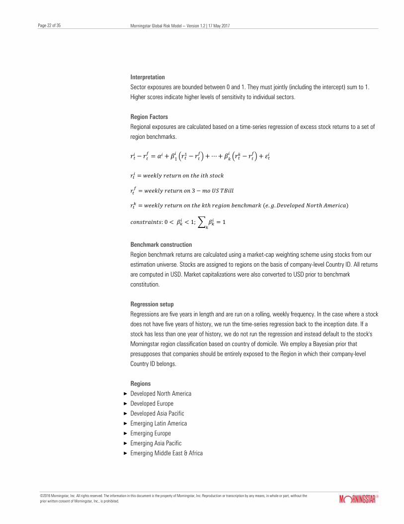
Region Factors

Regional exposures are calculated based on a time-series regression of excess stock returns to a set of

region benchmarks.



(𝑟𝑡1 − 𝑟𝑡

𝑓) + ⋯ + 𝛽𝑘

𝑖(𝑟𝑡

𝑘 − 𝑟𝑡𝑓

) + 휀𝑡𝑖

𝑟𝑡𝑖 = 𝑤𝑒𝑒𝑘𝑙𝑦 𝑟𝑒𝑡𝑢𝑟𝑛 𝑜𝑛 𝑡ℎ𝑒 𝑖𝑡ℎ 𝑠𝑡𝑜𝑐𝑘

𝑟𝑡𝑓

= 𝑤𝑒𝑒𝑘𝑙𝑦 𝑟𝑒𝑡𝑢𝑟𝑛 𝑜𝑛 3 − 𝑚𝑜 𝑈𝑆 𝑇𝐵𝑖𝑙𝑙 𝑟𝑡

𝑘 = 𝑤𝑒𝑒𝑘𝑙𝑦 𝑟𝑒𝑡𝑢𝑟𝑛 𝑜𝑛 𝑡ℎ𝑒 𝑘𝑡ℎ 𝑟𝑒𝑔𝑖𝑜𝑛 𝑏𝑒𝑛𝑐ℎ𝑚𝑎𝑟𝑘 (𝑒. 𝑔. 𝐷𝑒𝑣𝑒𝑙𝑜𝑝𝑒𝑑 𝑁𝑜𝑟𝑡ℎ 𝐴𝑚𝑒𝑟𝑖𝑐𝑎)

𝑐𝑜𝑛𝑠𝑡𝑟𝑎𝑖𝑛𝑡𝑠: 0 < 𝛽𝑘𝑖 < 1; ∑ 𝛽𝑘

𝑖

𝑘= 1

Benchmark construction

Region benchmark returns are calculated using a market-cap weighting scheme using stocks from our

estimation universe. Stocks are assigned to regions on the basis of company-level Country ID. All returns

are computed in USD. Market capitalizations were also converted to USD prior to benchmark

constitution.

Regression setup

Regressions are five years in length and are run on a rolling, weekly frequency. In the case where a stock

does not have five years of history, we run the time-series regression back to the inception date. If a

stock has less than one year of history, we do not run the regression and instead default to the stock's

Morningstar region classification based on country of domicile. We employ a Bayesian prior that

presupposes that companies should be entirely exposed to the Region in which their company-level

Country ID belongs.

Regions

× Developed North America

× Developed Europe

× Developed Asia Pacific

× Emerging Latin America

× Emerging Europe

× Emerging Asia Pacific

× Emerging Middle East & Africa





of 35

Page 23 of 35

Exhibit 7 Map of countries to regions Region Country List

Developed Asia Pacific Australia

Hong Kong

Japan

New Zealand

Singapore

Developed Europe Belgium

Switzerland

Germany

Denmark

Spain

Finland

France

United Kingdom

Greece

Ireland

Italy

Netherlands

Norway

Portugal

Sweden

Developed North America United States Canada

Emerging Europe Czech Republic

Hungary

Poland

Russian Federation

Turkey

Emerging Latin America Brazil

Chile

Colombia

Mexico

Peru

Emerging Middle East & Africa Egypt

Israel

Morocco South Africa


Interpretation

Region exposures are bounded between 0 and 1. They must jointly (including the intercept) sum to 1.

Higher scores indicate higher levels of sensitivity to individual regions.

Currency Factors

Currency exposures are calculated based on a time-series quantile regression of excess stock returns to

a set of exchange rates.



(𝑟𝑡1) + ⋯ + 𝛽𝑘

𝑖(𝑟𝑡

𝑘) + 휀𝑡𝑖

𝑟𝑡

𝑖 = 𝑤𝑒𝑒𝑘𝑙𝑦 𝑟𝑒𝑡𝑢𝑟𝑛 𝑜𝑛 𝑡ℎ𝑒 𝑖𝑡ℎ 𝑠𝑡𝑜𝑐𝑘

𝑟𝑡𝑓

= 𝑤𝑒𝑒𝑘𝑙𝑦 𝑟𝑒𝑡𝑢𝑟𝑛 𝑜𝑛 3 − 𝑚𝑜 𝑈𝑆 𝑇𝐵𝑖𝑙𝑙

𝑟𝑡𝑘 = 𝑤𝑒𝑒𝑘𝑙𝑦 𝑟𝑒𝑡𝑢𝑟𝑛 𝑜𝑛 𝑡ℎ𝑒 𝑘𝑡ℎ 𝑒𝑥𝑐ℎ𝑎𝑛𝑔𝑒 𝑟𝑎𝑡𝑒 𝑟𝑒𝑡𝑢𝑟𝑛 (𝑒. 𝑔. % 𝑐ℎ𝑎𝑛𝑔𝑒 𝑖𝑛

𝐸𝑈𝑅

𝑈𝑆𝐷)





of 35

Page 24 of 35

Regression Setup

Regressions are five years in length and are run on a rolling, weekly frequency. In the case where a

stock does not have five years of history, we run the time-series regression back to the inception date.

Stock returns are calculated in US dollar currency returns.

Currencies

× Euro

× Japanese Yen

× British Pound

× Swiss Franc

× Canadian Dollar

× Australian Dollar

× New Zealand Dollar

Interpretation

Currency exposures are unbounded, but generally fall between -1 and 1. Higher scores indicate higher

levels of sensitivity to individual exchange-rate fluctuations.





of 35

Page 25 of 35

Appendix C: Forecasted Statistics Definitions

Variance

Variance measures the dispersion of the forecasted return distribution. We calculate variance to help us

assess the level of uncertainty embedded in the expected return estimate. Higher variance indicates the

distribution is more spread out around the mean, so there is more uncertainty around the expected

return. A lower variance indicates the distribution is tightly located near the mean.

We generate variance from the second moment of the return distribution. The calculation is below:

𝑉𝑎𝑟𝑖𝑎𝑛𝑐𝑒(𝑋) = 𝜇2 − 𝜇12

Where:

𝜇𝑛 = 𝑡ℎ𝑒 𝑛𝑡ℎ 𝑟𝑎𝑤 𝑚𝑜𝑚𝑒𝑛𝑡 𝑜𝑓 𝑥 = 𝐸[𝑋𝑛]

𝜇1 = 𝐸[𝑤𝑡𝑇𝑋𝑡 exp(𝐴𝑆𝑡 + 𝑓)̅ − 𝑤𝑡

𝑇𝑋𝑡1 + 𝑤𝑡𝑇ϵ𝑡]

𝜇2 = 𝐸[(𝑤𝑡𝑇𝑋𝑡 exp(𝐴𝑆𝑡 + 𝑓̅) − 𝑤𝑡

𝑇𝑋𝑡1 + 𝑤𝑡𝑇ϵ𝑡)2]

𝑤 = (ℎ × 𝑛) 𝑚𝑎𝑡𝑟𝑖𝑥 𝑜𝑓 𝑝𝑜𝑟𝑡𝑓𝑜𝑙𝑖𝑜 𝑤𝑒𝑖𝑔ℎ𝑡𝑠

𝑋𝑡 = (𝑛 × 𝑚) 𝑚𝑎𝑡𝑟𝑖𝑥 𝑜𝑓 𝑠𝑡𝑜𝑐𝑘 𝑒𝑥𝑝𝑜𝑠𝑢𝑟𝑒𝑠 𝑡𝑜 𝑓𝑎𝑐𝑡𝑜𝑟𝑠 𝑎𝑡 𝑡𝑖𝑚𝑒 𝑡; 𝑚 = 36

𝐴 = (𝑚 × 𝑛) 𝑚𝑎𝑡𝑟𝑖𝑥 𝑜𝑓 𝑚𝑖𝑥𝑖𝑛𝑔 𝑐𝑜𝑒𝑓𝑓𝑖𝑐𝑖𝑒𝑛𝑡𝑠

𝑆 = (𝑛 × ℎ) 𝑚𝑎𝑡𝑟𝑖𝑥 𝑜𝑓 ℎ𝑖𝑠𝑡𝑜𝑟𝑖𝑐𝑎𝑙 𝑠𝑡𝑎𝑡𝑖𝑠𝑡𝑖𝑐𝑎𝑙𝑙𝑦 𝑖𝑛𝑑𝑒𝑝𝑒𝑛𝑑𝑒𝑛𝑡 𝑠𝑢𝑏 − 𝑓𝑎𝑐𝑡𝑜𝑟𝑠

𝑓𝑡 = (𝑛 × 1) 𝑣𝑒𝑐𝑡𝑜𝑟 𝑜𝑓 𝑠𝑡𝑜𝑐𝑘 𝑟𝑒𝑡𝑢𝑟𝑛𝑠 𝑎𝑡 𝑡𝑖𝑚𝑒 𝑡

𝜖𝑡 = (𝑛 × 1) 𝑣𝑒𝑐𝑡𝑜𝑟 𝑜𝑓 𝑒𝑟𝑟𝑜𝑟 𝑡𝑒𝑟𝑚𝑠 𝑎𝑡 𝑡𝑖𝑚𝑒 𝑡

Volatility

Volatility is another standard measure of dispersion for the forecasted return distribution. It is calculated

by taking the square root of the Variance as described above.

Skewness

Skewness measures the asymmetry of the forecasted return distribution. We calculate skewness to help

us understand the shape of the return distribution and where majority of the dispersion is located. A

positive skew indicates the return distribution is concentrated to the left of the expected return and vice

versa for a negative skew. Zero skew indicates the return distribution is perfectly symmetrical.

We generate skewness from the third moment of the return distribution. The calculation is below:

𝑆𝑘𝑒𝑤𝑛𝑒𝑠𝑠(𝑋) = 𝜇3 − 3𝜇1𝜇2 + 3𝜇1

3 − 𝜇12

(𝜇2 − 𝜇12)1.5

Where:






of 35

Page 26 of 35







𝑤 = (ℎ × 𝑛) 𝑚𝑎𝑡𝑟𝑖𝑥 𝑜𝑓 𝑝𝑜𝑟𝑡𝑓𝑜𝑙𝑖𝑜 𝑤𝑒𝑖𝑔ℎ𝑡𝑠 (? )






Kurtosis

Kurtosis measures the tails of the forecasted return distribution. While many risk models assume a

normal distribution, our model does not and kurtosis helps describe how a security may behave in

extreme market turmoil. We calculate kurtosis relative to the normal distribution, which has a score of 0.

A return distribution with kurtosis less than 3 indicates that the tails are narrower than the normal

distribution. Therefore, relative to a normal distribution forecast, we expect fewer extreme events to

occur. The reverse is true for distributions with a kurtosis score greater than 3.

We generate kurtosis from the fourth moment of the return distribution. The calculation is below:

𝐾𝑢𝑟𝑡𝑜𝑠𝑖𝑠(𝑋) = 𝜇4 − 4𝜇1𝜇3 + 6𝜇1

2𝜇2 − 4𝜇13𝜇1 − 𝜇1

4

(𝜇2 − 𝜇12)2

Where:










𝑤 = (ℎ × 𝑛) 𝑚𝑎𝑡𝑟𝑖𝑥 𝑜𝑓 𝑝𝑜𝑟𝑡𝑓𝑜𝑙𝑖𝑜 𝑤𝑒𝑖𝑔ℎ𝑡𝑠 (? )






Probability of Negative Return

Probability of Negative Return is the percentage of the return distribution below a 0% return. This risk

statistic informs us of the location of the return forecast. A number close to 0 indicates the forecasted





of 35

Page 27 of 35

return profile is almost entire positive. We have high confidence the security will have a positive return

over the associated time period. Whereas, a number close to 1 indicates the forecasted return profile is

almost entirely negative and we have high confidence the security will lose value over the same time

period.

Value at Risk

Value at Risk, VAR, is the expected return at the lowest 1st percentile of the return distribution. We

calculate VAR to understand the magnitude of the tail forecast. A number close to -1 indicates the

security will be severely impacted if the 1st percentile of worst case scenarios occurs and will lose

almost its entire value. A number close to 0 indicates the security will come away relatively unscathed

during the same scenario.

CVAR

Conditional Value-at-Risk, CVAR, is the expected loss in the worst 1% of cases. Intuitively, CVAR

answers the question, what happens if a crisis is so severe, the 1st percentile is exceeded? To calculate,

we isolate the returns in the bottom 1st percentile of the distribution and calculate the average return.

CVAR represents the expected return in the worst case situation.

Tracking Error

Tracking Error measures the dispersion of a fund’s forecasted return distribution in excess of a

benchmark. Historical Tracking Error is usually measured using the following formula:

𝑇𝐸 = √∑ (𝑅𝑝 − 𝑅𝐵)2𝑁

𝑖=1

𝑁 − 1

Essentially, Historical Tracking Error is the standard deviation of a fund or portfolio’s return stream, 𝑅𝑝, in

excess of a benchmark, 𝑅𝐵.

Using the Risk Model, we can also produce forecasted Tracking Error. In order to calculate this forecast,

we calculate net factor exposures for the fund above/below the benchmark. Then, we forecast variance

for the fund using the net exposures. The net exposure represents the active bets that the fund may be

taking compared to the benchmark. Currently, the forecasted Tracking Error data point is calculated for

every fund using the fund’s primary prospectus benchmark.





of 35

Page 28 of 35

𝑇𝑟𝑎𝑐𝑘𝑖𝑛𝑔 𝐸𝑟𝑟𝑜𝑟(𝑋) = √𝜇2 − 𝜇12

Where:


𝜇1 = 𝐸[(𝑤𝑡𝑇,𝐹 − 𝑤𝑡

𝑇,𝐵)𝑋𝑡 exp(𝐴𝑆𝑡 + 𝑓̅) − (𝑤𝑡𝑇,𝐹 − 𝑤𝑡

𝑇,𝐵)𝑋𝑡1 + (𝑤𝑡𝑇,𝐹 − 𝑤𝑡

𝑇,𝐵)ϵ𝑡]

𝜇2 = 𝐸[(𝑤𝑡𝑇,𝐹 − 𝑤𝑡

𝑇,𝐵)𝑋𝑡 exp(𝐴𝑆𝑡 + 𝑓̅) − (𝑤𝑡𝑇,𝐹 − 𝑤𝑡

𝑇,𝐵)𝑋𝑡1 + (𝑤𝑡𝑇,𝐹 − 𝑤𝑡

𝑇,𝐵)ϵ𝑡)2]

𝑤𝐹 = (ℎ × 𝑛) 𝑚𝑎𝑡𝑟𝑖𝑥 𝑜𝑓 𝑓𝑢𝑛𝑑 𝑝𝑜𝑟𝑡𝑓𝑜𝑙𝑖𝑜 𝑤𝑒𝑖𝑔ℎ𝑡𝑠

𝑤𝐵 = (ℎ × 𝑛) 𝑚𝑎𝑡𝑟𝑖𝑥 𝑜𝑓 𝑏𝑒𝑛𝑐ℎ𝑚𝑎𝑟𝑘 𝑤𝑒𝑖𝑔ℎ𝑡𝑠










of 35

Page 29 of 35

Appendix D: Independent Component Analysis

Independent Component Analysis (ICA) is a technique that was developed to solve the problem of blind

source separation―an example of which is known as the cocktail party problem. In the cocktail party

scenario an observer has set up several recording devices throughout a cocktail party to listen to the

attendees. The voices are all jumbled together in the hubbub. The observer would like to extract the

individual voices from the recordings without any additional knowledge..

ICA solves the cocktail party problem by linearly transforming the time series of recordings into a

new set of time series which are each statistically independent from each other. In other words, these

new time series are simply weighted sums of the original time series and the weights are chosen in

such a way that none of the new time series have any mutual information―that is that there is no

knowledge to be gained about any time series by looking at any other time series. In the cocktail party

problem, these independent time series, or “sources”, should represent individual voices. This mutual

information criterion maps naturally to speakers―supposing one person in one part of the room is

saying something at some particular instant should tell us nothing about what the other speakers are

saying at that same instant.

In finance we care about returns. We cannot directly observe the independent latent sources of those

returns, but we can observe asset returns―these act like our recording devices. Performing ICA on asset

returns delivers us a set of statistically independent drivers of those returns that are linear combinations

of the original returns. This makes it easy to transform returns into sources or vice versa. So the

assumption is that there are a collection of independent sources which drive returns. There are two

potential intuitive justifications for this assumption. First, some drivers clearly are independent―for

instance natural disasters and technology innovation are truly independent. Second, the assumption

that returns are a linear combination of univariate time series is a convenient and makes modeling

possible, we can see this in the large collection of workable risk models which use techniques like factor

analysis and PCA. Independence is the natural criteria which allows for rich univariate models.

The objective of ICA is to take an original m × h matrix 𝐗 and find the weights A, that can be multiplied

by the statistically independent sources S, to recover our original data, X, so X = AS. The matrix A is

sometimes referred to as the mixing matrix.

There are several algorithms for performing ICA. These algorithms have inter-relationships and are

equivalent with the addition of some technical criteria. There is a maximum likelihood formalism of ICA

called Maximum Likelihood ICA in which a likelihood function for the mixing matrix is written down and

standard ML techniques are employed. There is a technique called InfoMax which measures the joint

entropy of the signals, and uses the fact that a set of signals which has maximum joint entropy is

mutually independent. There is a technique called FastICA, which is independently derived but is similar

to using stochastic gradient descent to maximize the likelihood, with a time-varying learning rate

resulting in a fast solution. We use FastICA.





of 35

Page 30 of 35

Suppose we know the pdf of the univariate sources by assumption. Call these pdfs fi. Suppose that

W = (w1, … wm)⊤ is the matrix A−1. Then the log likelihood will take the form:

𝐿 = ∑ ∑ 𝑙𝑜𝑔 𝑓𝑖(𝑤𝑖⊤𝑥𝑡)

𝑚

𝑖=1

ℎ

𝑡=1

+ ℎ 𝑙𝑜𝑔 | 𝑑𝑒𝑡 𝑊|

The last term here is from the Jacobian to transform the random variables.

This formalism assumes we know the pdf of the univariate sources – of course this is not known in

general. The sum of a collection of independent variables (given some nice properties like finite variance)

will tend to be normally distributed thanks to the central limit theorem. Suppose we have a fixed

unknown S and A, and we want to estimate one of the wi. Because of the central limit theorem, wi⊤AS

will necessarily be more normal than all of the s unless it happens to be equal to one of them. So the

collection of weights which maximizes the non-normality of wi⊤AS will recover the original source. It

happens that for many purposes several high-kurtosis pdfs work approximately equivalently well to find

non-normal sources.

The FastICA algorithm we use employs an approximation of the pdf shown below.

𝑓(𝑥) =1

𝛼𝑙𝑜𝑔 𝑐𝑜𝑠ℎ(𝛼𝑥)

This approximation tends to be a more robust measure of non-normality than other common measures,

e.g. kurtosis.





of 35

Page 31 of 35

Appendix E: Generalized Autoregressive Conditional Heteroskedastic Normal Inverse Gaussian

We use Normal Inverse Gaussian (NIG) distribution to model the independent univariate time series.

By assumption both the idiosyncratic risk and independent components are mutually independent.

The NIG distribution is a special case of generalized hyperbolic (GH) distributions, and which have five

parameters to capture the heaviness and skewness of a data set. It is possible to show that setting

λ= -1/2 in the GH distribution, we obtain an NIG distribution. We estimate the NIG parameters with

maximum likelihood, relying on the independence property to assume that the sum of the log-likelihoods

is the log-likelihood of the joint distribution.

The density expression for the NIG distribution is:

𝑓(𝑥; 𝛼, 𝛽, 𝜇, 𝛿) =𝛼𝛿

𝜋𝑒𝛿√𝛼2−𝛽2+𝛽(𝑥−𝜇)

𝑲1 (𝛼√𝛿2 + (𝑥 − 𝜇)2)

√𝛿2 + (𝑥 − 𝜇)2

The distribution has the following parameters:

μ: location parameter, for real μ

δ: scale parameter, for non-negative δ

α: tail heaviness parameter, and

β: asymmetry parameter for 0 ≤ |β| ≤ α.

We also use an auxiliary parameter γ = √α2 − β2.

Here 𝐊1 is the modified Bessel function of the third order and index 1.

If x is NIG distributed, the shape parameters for a random variable s of the distribution are

𝐸[𝑠] = 𝜇 +𝛿𝛽

√𝛼2 − 𝛽2= 𝜇 +

𝛿𝛽

𝛾

𝑉𝑎𝑟[𝑠] =𝛿𝛼2

(√𝛼2 − 𝛽2)3 =

𝛿𝛼2

𝛾3

𝑆𝑘𝑒𝑤[𝑠] =3𝛽

𝛼√𝛿√𝛼2 − 𝛽2

=3𝛽

𝛼√𝛿𝛾

𝐾𝑢𝑟[𝑠] =3(1 + 4𝛽2/𝛼2 )

𝛿√𝛼2 − 𝛽2+ 3 =

3(1 + 4𝛽2/𝛼2 )

𝛿𝛾+ 3

NIG models are by themselves insufficient to characterize the univariate time series. The volatility of real

return series is not constant over time, whereas the second moment for f above, which does not include

any autocorrelation, is constant. We want to capture behavior typical of financial markets, such as

volatility clustering and the auto-correlated volatilities. Furthermore we want a model with few





of 35

Page 32 of 35

parameters which is likely to be numerically robust. This model is in essence a simplified version of the

model in Jensen and Lunde (2001) as we outline below. The simplification makes the model robust for

estimation purposes.

We use a Generalized Autoregressive Conditional Heteroskedasticity (GARCH) process to model the

dynamic nature of our NIG distributed returns. This work is related to existing GARCH-NIG and ARCH-

NIG models. Work which fits GARCH(1,1) models, e.g. Jensen and Lunde (2001) typically finds the

volatility update equation which has the following form

𝜎𝑡+12 = 𝑎 + 𝑏𝜎𝑡

2 + 𝑐𝜖𝑡2 .

Start by re-parameterizing the NIG distribution:

�̅� = 𝛿𝛼

�̅� = 𝛿𝛽

�̅� = √�̅�2

− �̅�2

= 𝛿𝛾

This gives an alternative density function g and we say a random variable is "NIG"(α ̅,β ̅,μ,δ) distributed

if it has this following density.

𝑔(𝑥; �̅�, 𝛽,̅ 𝜇, 𝛿) =�̅�

𝜋𝛿𝑒𝑥𝑝 (�̅� + �̅�

(𝑥 − 𝜇)

𝛿)

𝑲1 (�̅�√1 +(𝑥 − 𝜇)2

𝛿2 )

√1 +(𝑥 − 𝜇)2

𝛿2

Given this rewrite, if s is a random variable we can write the conditional moments (omitting subscripts)

as follows. Note that the skewness and kurtosis can be expressed only in terms ofα̅, β̅ and γ̅.

𝐸[𝑠] = 𝜇 +𝛿𝛽

𝛾= 𝜇 +

𝛿�̅�

�̅�

𝑉𝑎𝑟[𝑠] =𝛿𝛼2

𝛾3 = 𝛿4𝛼2

�̅�3 =𝛿2�̅�2

�̅�3

𝑆𝑘𝑒𝑤[𝑠] =3𝛽

𝛼√𝛿𝛾=

3�̅�

�̅�√�̅�

𝐾𝑢𝑟[𝑠] =3(1 + 4𝛽2/𝛼2 )

𝛿𝛾+ 3 =

3 (1 + 4𝛽2

/�̅�2 )

�̅�+ 3

We use a GARCH approximation, and allow the volatility σ to progress as follows.

𝜎𝑡2 = 𝑎 + 𝑏𝑏𝜎𝑡−1

2 + (1 − 𝜆)𝜖2𝑡−1𝑐𝜖𝑡−1

2





of 35

Page 33 of 35

We then set:

𝑠𝑡 = 𝜇𝑡 +√�̅��̅�

�̅�𝜎𝑡 + 𝜎𝑡𝜂𝑡

𝜂𝑡~ 𝑁𝐼𝐺(�̅�, �̅�, − √�̅��̅�

�̅�,�̅�3/2

�̅�)

𝜖𝑡 = 𝜎𝑡𝜂𝑡

Here st is a factor or residual innovation.

Why this parameterization? First notice that now everywhere that x occurs, it occurs in the context of

(x − μ)/δ. This means that if X ~ NIG(α̅, β̅, μ, δ), then (X − μ)/δ ~ NIG(α ̅, β ̅, 0,1). It then becomes

possible to push all the time-varying portion of the distribution into δ, and leave α̅, β̅ constant. The idea

is to give ηt mean of 0 and variance of 1, which comes about as follows:

𝐸[𝜂𝑡] = 𝜇𝑡 +�̅�

�̅�

𝛿𝑡

√1 − (�̅� �̅�⁄ )2

= − √�̅��̅�

�̅�+

�̅�

�̅�

�̅�3/2 �̅�⁄

√1 − (�̅� �̅�⁄ )2

= 0

For variance we have:

𝑉𝐴𝑅[𝜂𝑡] =𝛿𝛼2

𝛾3=

𝛿4𝛼2

�̅�3=

𝛿2�̅�2

�̅�3

= (�̅�

32

�̅�)

2

�̅�2

�̅�3

= 1

This means in turn that:

𝑠𝑡~ 𝑁𝐼𝐺(�̅�, �̅�, 𝜇𝑡, 𝜎𝑡

�̅�32

�̅�)

𝑉𝐴𝑅[𝑠𝑡|𝜎𝑡−1] = 𝜎𝑡

2 = 𝑎 + 𝑏𝜎𝑡−12 + 𝑐𝜖𝑡−1

2

𝐸[𝑠𝑡|𝜎𝑡−1] = 𝜇𝑡 + 𝜎𝑡 √�̅��̅�

�̅�= 0





of 35

Page 34 of 35

For most of our time series we subtract the mean from the dataset before fitting the distribution and so

essentially assume that the unconditional expected return is zero, which gives that:

𝜇𝑡 = −𝜎𝑡 √�̅��̅�

�̅�

Alongside the pdf from the last section, a log-likelihood for particular sequences of volatilities and NIG

parameters is straightforward, and the parameters of the distribution can be estimated with the

following steps:

1. Take as inputs s0, … , sT, and an initial guess for σ0, γ̅, α̅, β̅ (we set μ0 from d below for time 0).

2. Repeat for all i > 0:

a. ϵi−1 = si−1 − σi−1√γ̅β̅

α̅− μi−1 = si−1

b. 𝜎𝑖2 = 𝑎 + 𝑏𝜎𝑖−1

2 + 𝑐𝜖𝑖−12

c. μi = −σi √γ̅β̅

α̅

3. Calculate the log-likelihood as:

ℒ(�̅�, �̅�; 𝜎0, 𝒔) = ∑ 𝑙𝑜𝑔 𝑔(𝑠𝑖; �̅�, 𝛽,̅ 𝜇𝑖 , 𝜎𝑖

�̅�3/2

�̅�)

𝑇

𝑖=0

Note that if E[st] is assumed to be zero, then the future volatility estimate depends only on the historical

returns and volatility, and the μi are only required to calculate the likelihood. We can then maximize this

log-likelihood with a suitable optimizer, we use BFGS. K





of 35

Page 35 of 35

About Morningstar® Quantitative Research™

Morningstar Quantitative Research is dedicated to developing innovative statistical models and data

points, including the Quantitative Equity Ratings and the Global Risk Model.

For More Information

+1 312 244-7541

[email protected]

?

22 West Washington Street

Chicago, IL 60602 USA

© Morningstar 2016. All Rights Reserved. The information, data, analyses and opinions presented herein do not constitute

investment advice; are provided solely for informational purposes and therefore are not an offer to buy or sell a security; and are

not warranted to be correct, complete or accurate. The opinions expressed are as of the date written and are subject to change

without notice. Except as otherwise required by law, Morningstar shall not be responsible for any trading decisions, damages or

other losses resulting from, or related to, the information, data, analyses or opinions or their use. The information contained herein

is the proprietary property of Morningstar and may not be reproduced, in whole or in part, or used in any manner, without the prior

written consent of Morningstar. To order reprints, call +1 312-696-6100. To license the research, call +1 312-696-6869.

Morningstar Global Risk Model MethodologyIn essence, the model seeks to identify a small number of...

Documents

Transcript of Morningstar Global Risk Model MethodologyIn essence, the model seeks to identify a small number of...