Moritz Diehl Optimization in Engineering Center (OPTEC ... · Optimization in Engineering Center...
53
Numerical Optimal Control Moritz Diehl Optimization in Engineering Center (OPTEC) & Electrical Engineering Department (ESAT) K.U. Leuven Belgium
-
Upload
nguyenthien -
Category
Documents
-
view
227 -
download
1
Transcript of Moritz Diehl Optimization in Engineering Center (OPTEC ... · Optimization in Engineering Center...

Numerical Optimal ControlMoritz Diehl
Optimization in Engineering Center (OPTEC)
& Electrical Engineering Department (ESAT)
K.U. Leuven
Belgium

Simplified Optimal Control Problem in ODE
terminalconstraint r(x(T )) ≥ 0
6path constraints h(x, u) ≥ 0
initial valuex0 r
states x(t)
controls u(t)-p
0 tpT
minimizex(·), u(·)
∫ T
0
L(x(t), u(t)) dt + E (x(T ))
subject to
x(0) − x0 = 0, (fixed initial value)x(t)−f(x(t), u(t)) = 0, t ∈ [0, T ], (ODE model)
h(x(t), u(t)) ≥ 0, t ∈ [0, T ], (path constraints)r (x(T )) ≥ 0 (terminal constraints).

More general optimal control problems
Many features left out here for simplicity of presentation:
• multiple dynamic stages
• differential algebraic equations (DAE) instead of ODE
• explicit time dependence
• constant design parameters
• multipoint constraints r(x(t0), x(t1), . . . , x(tend)) = 0

Optimal Control Family Tree
Three basic families:
• Hamilton-Jacobi-Bellmann equation / dynamic programming
• Indirect Methods / calculus of variations / Pontryagin
• Direct Methods (control discretization)
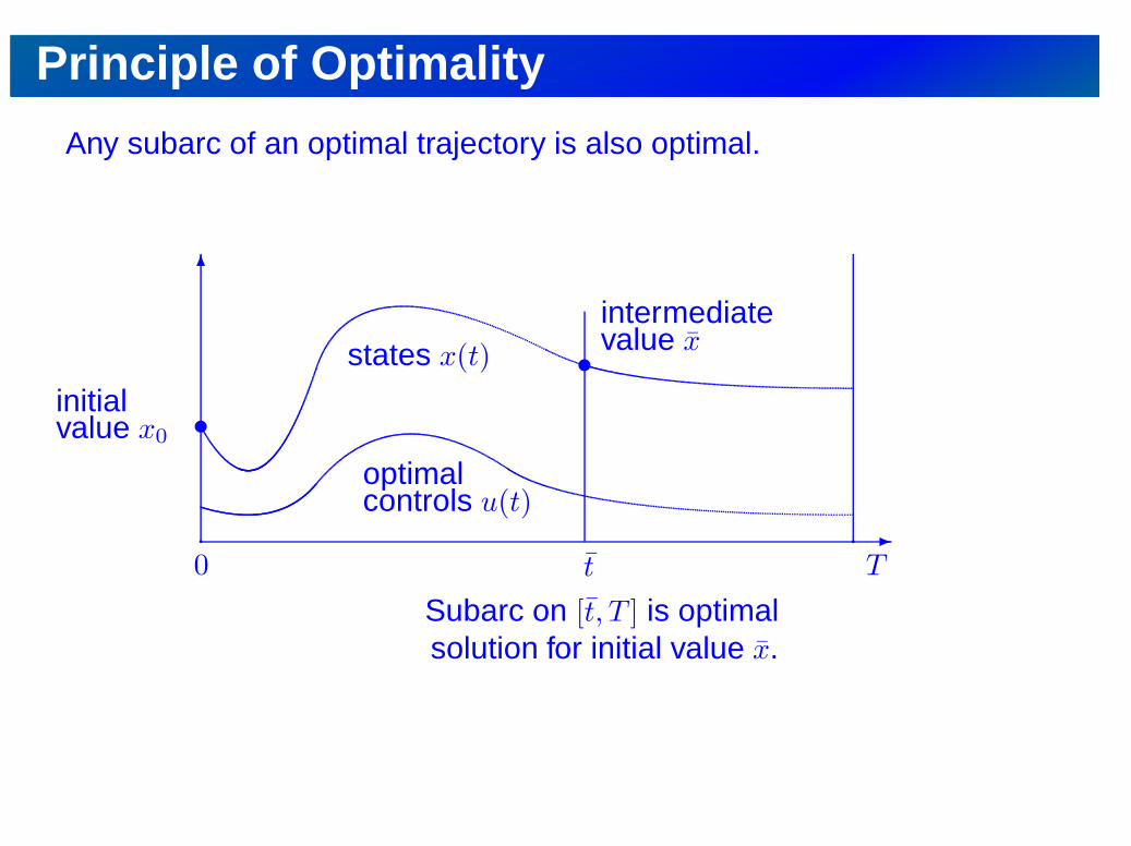
Principle of Optimality
Any subarc of an optimal trajectory is also optimal.
6intermediatevalue x
s
initialvalue x0
s
states x(t)
optimalcontrols u(t)
-p
0 tp
T
Subarc on [t, T ] is optimalsolution for initial value x.

Dynamic Programming Cost-to-go
IDEA:
• Introduce optimal-cost-to-go function on [t, T ]
J(x, t) := minx,u
∫ T
t
L(x, u)dt + E(x(T )) s.t. x(t) = x, . . .
• Introduce grid 0 = t0 < . . . < tN = T .
• Use principle of optimality on intervals [tk, tk+1]:
J(xk, tk) = minx,u
∫ tk+1
tk
L(x, u)dt + J(x(tk+1), tk+1) s.t. x(tk) = xk, . . .
xkr x(tk+1)r
-tk+1tk
p
T

Dynamic Programming RecursionStarting from J(x, tN ) = E(x), compute recursively backwards,for k = N − 1, . . . , 0
J(xk, tk) := minx,u
∫ tk+1
tk
L(x, u)dt + J(x(tk+1), tk+1) s.t. x(tk) = xk, . . .
by solution of short horizon problems for all possible xk and tabulationin state space.

Dynamic Programming RecursionStarting from J(x, tN ) = E(x), compute recursively backwards,for k = N − 1, . . . , 0
J(xk, tk) := minx,u
∫ tk+1
tk
L(x, u)dt + J(x(tk+1), tk+1) s.t. x(tk) = xk, . . .
by solution of short horizon problems for all possible xk and tabulationin state space.
@@@R
6
J(·, tN )
xN
@@@R
6
J(·, tN−1)
xN−1
· · ·
@@@R
6
J(·, t0)
x0

Hamilton-Jacobi-Bellman (HJB) Equation
Dynamic Programming with infinitely small timesteps leads toHamilton-Jacobi-Bellman (HJB) Equation :
−∂J
∂t(x, t) = min
u
(
L(x, u) +∂J
∂x(x, t)f(x, u)
)
s.t. h(x, u) ≥ 0.
Solve this partial differential equation (PDE) backwards for t ∈ [0, T ],starting at the end of the horizon with
J(x, T ) = E(x).
NOTE: Optimal controls for state x at time t are obtained from
u∗(x, t) = arg minu
(
L(x, u) +∂J
∂x(x, t)f(x, u)
)
s.t. h(x, u) ≥ 0.
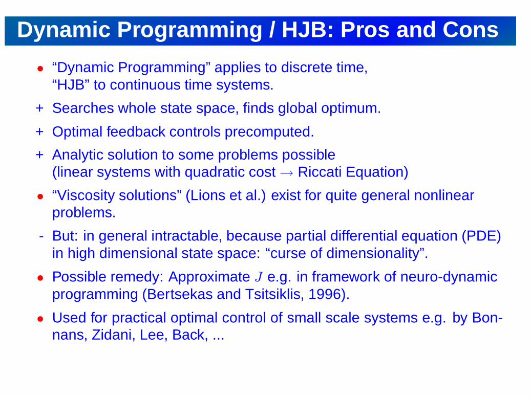
Dynamic Programming / HJB: Pros and Cons
• “Dynamic Programming” applies to discrete time,“HJB” to continuous time systems.
+ Searches whole state space, finds global optimum.
+ Optimal feedback controls precomputed.
+ Analytic solution to some problems possible(linear systems with quadratic cost → Riccati Equation)
• “Viscosity solutions” (Lions et al.) exist for quite general nonlinearproblems.
- But: in general intractable, because partial differential equation (PDE)in high dimensional state space: “curse of dimensionality”.
• Possible remedy: Approximate J e.g. in framework of neuro-dynamicprogramming (Bertsekas and Tsitsiklis, 1996).
• Used for practical optimal control of small scale systems e.g. by Bon-nans, Zidani, Lee, Back, ...

Indirect MethodsFor simplicity, regard only problem without inequality constraints:
terminalcost E(x(T ))
6
initial valuex0 r
states x(t)
controls u(t)-p
0 tpT
minimizex(·), u(·)
∫ T
0
L(x(t), u(t)) dt + E (x(T ))
subject to
x(0) − x0 = 0, (fixed initial value)x(t)−f(x(t), u(t)) = 0, t ∈ [0, T ]. (ODE model)

Pontryagin’s Minimum Principle
OBSERVATION: In HJB, optimal controls
u∗(t) = arg minu
(
L(x, u) +∂J
∂x(x, t)f(x, u)
)
depend only on derivative ∂J∂x
(x, t), not on J itself!
IDEA: Introduce adjoint variables λ(t) = ∂J∂x
(x(t), t)T ∈ Rnx and get
controls from Pontryagin’s Minimum Principle
u∗(t, x, λ) = arg minu
L(x, u) + λT f(x, u)︸ ︷︷ ︸
Hamiltonian =:H(x,u,λ)
QUESTION: How to obtain λ(t)?
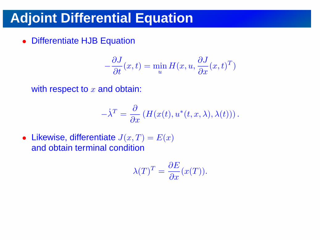
Adjoint Differential Equation
• Differentiate HJB Equation
−∂J
∂t(x, t) = min
uH(x, u,
∂J
∂x(x, t)T )
with respect to x and obtain:
−λT =∂
∂x(H(x(t), u∗(t, x, λ), λ(t))) .
• Likewise, differentiate J(x, T ) = E(x)and obtain terminal condition
λ(T )T =∂E
∂x(x(T )).

How to obtain explicit expression for controls?
• In simplest case,
u∗(t) = arg minu
H(x(t), u, λ(t))
is defined by∂H
∂u(x(t), u∗(t), λ(t)) = 0
(Calculus of Variations, Euler-Lagrange).
• In presence of path constraints, expression for u∗(t) changes wheneveractive constraints change. This leads to state dependent switches.
• If minimum of Hamiltonian locally not unique, “singular arcs” occur.Treatment needs higher order derivatives of H.

Necessary Optimality Conditions
Summarize optimality conditions as boundary value problem :
x(0) = x0, (initial value)x(t) = f(x(t), u∗(t)) t ∈ [0, T ], (ODE model)
−λ(t) = ∂H∂x
(x(t), u∗(t), λ(t))T , t ∈ [0, T ], (adjoint equations)u∗(t) = arg min
uH(x(t), u, λ(t)), t ∈ [0, T ], (minimum principle)
λ(T ) = ∂E∂x
(x(T ))T . (adjoint final value).
Solve with so called
• gradient methods,
• shooting methods, or
• collocation.

Indirect Methods: Pros and Cons• “First optimize, then discretize”
+ Boundary value problem with only 2 × nx ODE.
+ Can treat large scale systems.
- Only necessary conditions for local optimality.
- Need explicit expression for u∗(t), singular arcs difficult to treat.
- ODE strongly nonlinear and unstable.
- Inequalities lead to ODE with state dependent switches.
(possible remedy: Use interior point method in function spaceinequalities, e.g. Weiser and Deuflhard, Bonnans andLaurent-Varin)
• Used for optimal control e.g. by Srinivasan and Bonvin, Oberle,...
Direct Methods• “First discretize, then optimize”
• Transcribe infinite problem into finite dimensional, NonlinearProgramming Problem (NLP) , and solve NLP.
Pros and Cons:
+ Can use state-of-the-art methods for NLP solution.
+ Can treat inequality constraints and multipoint constraints mucheasier.
- Obtains only suboptimal/approximate solution.
• Nowadays most commonly used methods due to their easyapplicability and robustness.

Direct Methods OverviewWe treat three direct methods:
• Direct Single Shooting (sequential simulation and optimization)
• Direct Collocation (simultaneous simulation and optimization)
• Direct Multiple Shooting (simultaneous resp. hybrid)

Direct Single Shooting [Hicks, Ray 1971; Sargent, Sullivan 1977]
Discretize controls u(t) on fixed grid 0 = t0 < t1 < . . . < tN = T, regardstates x(t) on [0, T ] as dependent variables.
6
x0r
states x(t; q)
discretized controls u(t; q)
q0
q1
qN−1 -p
0 tp
T
Use numerical integration to obtain state as function x(t; q) of finitely manycontrol parameters q = (q0, q1, . . . , qN−1)

NLP in Direct Single Shooting
After control discretization and numerical ODE solution, obtain NLP:
minimizeq
∫ T
0
L(x(t; q), u(t; q)) dt + E (x(T ; q))
subject to
h(x(ti; q), u(ti; q)) ≥ 0, i = 0, . . . , N, (discretized path constraints)r (x(T ; q)) ≥ 0. (terminal constraints)
Solve with finite dimensional optimization solver, e.g. SequentialQuadratic Programming (SQP).

Solution by Standard SQP
Summarize problem as
minq
F (q) s.t. H(q) ≥ 0.
Solve e.g. by Sequential Quadratic Programming (SQP), starting withguess q0 for controls. k := 0
1. Evaluate F (qk), H(qk) by ODE solution, and derivatives!
2. Compute correction ∆qk by solution of QP:
min∆q
∇F (qk)T ∆q +1
2∆qT Ak∆q s.t. H(qk) + ∇H(qk)T ∆q ≥ 0.
3. Perform step qk+1 = qk + αk∆qk with step length αk determinedby line search.
ODE SensitivitiesHow to compute the sensitivity
∂x(t; q)
∂q
of a numerical ODE solution x(t; q) with respect to the controls q?Four ways:
1. External Numerical Differentiation (END)
2. Variational Differential Equations
3. Automatic Differentiation
4. Internal Numerical Differentiation (IND)

1 - External Numerical Differentiation (END)
Perturb q and call integrator several times to compute derivatives byfinite differences:
x(t; q + ǫei) − x(t; q)
ǫ
Very easy to implement, but several problems:
• Relatively expensive, have overhead of error control for eachvaried trajectory.
• Due to adaptivity, each call might have different discretizationgrids: output x(t; q) is not differentiable!
• How to chose perturbation stepsize? Rule of thumb: ǫ =√
TOLif TOL is integrator tolerance.
• Looses half the digits of accuracy. If integrator accuracy has(typical) value of TOL = 10−4, derivative has only two validdigits!
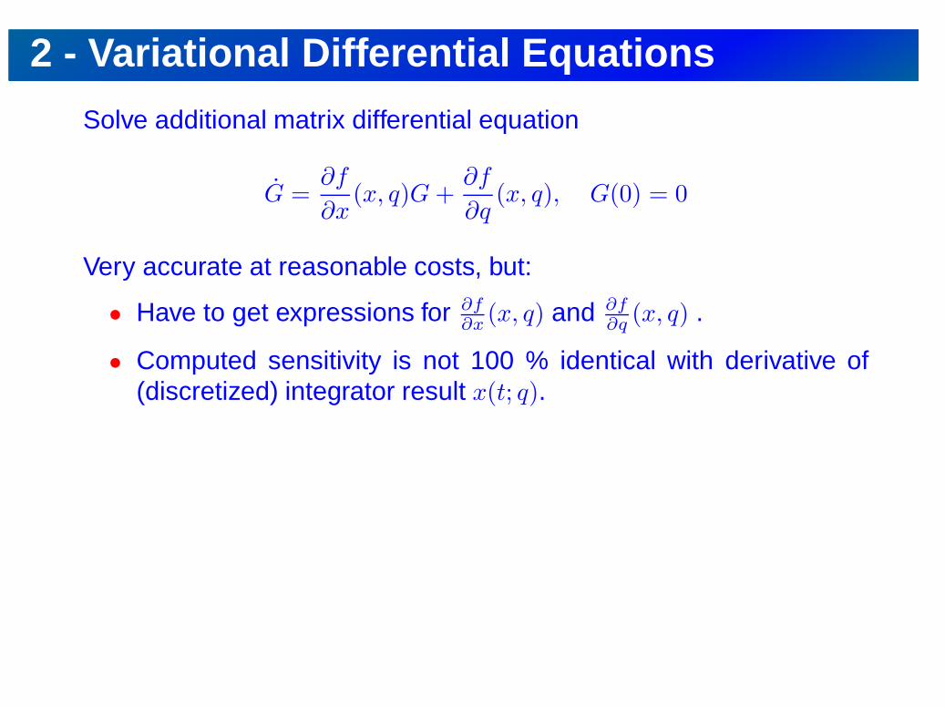
2 - Variational Differential Equations
Solve additional matrix differential equation
G =∂f
∂x(x, q)G +
∂f
∂q(x, q), G(0) = 0
Very accurate at reasonable costs, but:
• Have to get expressions for ∂f∂x
(x, q) and ∂f∂q
(x, q) .
• Computed sensitivity is not 100 % identical with derivative of(discretized) integrator result x(t; q).

3- Automatic Differentiation (AD)
Use Automatic Differentiation (AD): differentiate each step of the in-tegration scheme.Illustration: AD of Euler:
G(tk + h) = G(tk) + h∂f
∂x(x(tk), q)G(tk) + h
∂f
∂q(x(tk), q)
Up to machine precision 100 % identical with derivative of numericalsolution x(t; q), but:
• Integrator and right hand side (f(x, q)) need be in same or com-patible computer languages (e.g. C++ when using ADOL-C)

4 - Internal Numerical Differentiation (IND)
Like END, but evaluate simultaneously all perturbed trajectories xi
with frozen discretization grid.Illustration: IND of Euler:
xi(tk + hk) = xi(tk) + hkf(xi(tk), q + ǫei)
Up to round-off and linearization errors identical with derivative ofnumerical x(t; q), but:
• How to chose perturbation stepsize? Rule of thumb: ǫ =√
PRECif PREC is machine precision .
Note: adaptivity of nominal trajectory only, reuse of matrix factoriza-tion in implicit methods, so not only more accurate, but also cheaperthan END.

Numerical Test Problem
minimizex(·), u(·)
∫ 3
0
x(t)2 + u(t)2 dt
subject to
x(0) = x0, (initial value)x = (1 + x)x + u, t ∈ [0, 3], (ODE model)
1 − x(t)
1 + x(t)
1 − u(t)
1 + u(t)
≥
0
0
0
0
, t ∈ [0, 3], (bounds)
x(3) = 0. (zero terminal constraint).
Remark: Uncontrollable growth for (1 + x0)x0 − 1 ≥ 0 ⇔ x0 ≥ 0.618.

Single Shooting Optimization for x0 = 0.05
• Choose N = 30 equal control intervals.
• Initialize with steady state controls u(t) ≡ 0.
• Initial value x0 = 0.05 is the maximum possible,because initial trajectory explodes otherwise.

Single Shooting: First Iteration

Single Shooting: 2nd Iteration

Single Shooting: 3rd Iteration
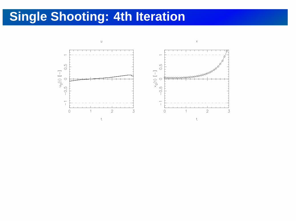
Single Shooting: 4th Iteration

Single Shooting: 5th Iteration

Single Shooting: 6th Iteration

Single Shooting: 7th Iteration and Solution

Direct Single Shooting: Pros and Cons
• Sequential simulation and optimization.
+ Can use state-of-the-art ODE/DAE solvers.
+ Few degrees of freedom even for large ODE/DAE systems.
+ Active set changes easily treated.
+ Need only initial guess for controls q.
- Cannot use knowledge of x in initialization (e.g. in trackingproblems).
- ODE solution x(t; q) can depend very nonlinearly on q.
- Unstable systems difficult to treat.
• Often used in engineering applications e.g. in packages gOPT(PSE), DYOS (Marquardt), ...

Direct Collocation (Sketch) [Tsang et al. 1975]
• Discretize controls and states on fine grid with node values si ≈ x(ti).
• Replace infinite ODE
0 = x(t) − f(x(t), u(t)), t ∈ [0, T ]
by finitely many equality constraints
ci(qi, si, si+1) = 0, i = 0, . . . , N − 1,
e.g. ci(qi, si, si+1) := si+1−si
ti+1−ti
− f(
si+si+1
2 , qi
)
• Approximate also integrals, e.g.
∫ ti+1
ti
L(x(t), u(t))dt ≈ li(qi, si, si+1) := L
(si + si+1
2, qi
)
(ti+1 − ti)

NLP in Direct CollocationAfter discretization obtain large scale, but sparse NLP:
minimizes, q
N−1∑
i=0
li(qi, si, si+1) + E (sN )
subject to
s0 − x0 = 0, (fixed initial value)ci(qi, si, si+1) = 0, i = 0, . . . , N − 1, (discretized ODE model)
h(si, qi) ≥ 0, i = 0, . . . , N, (discretized path constraints)r (sN ) ≥ 0. (terminal constraints)
Solve e.g. with SQP method for sparse problems.

What is a sparse NLP?
General NLP:
minw
F (w) s.t.
{
G(w) = 0,
H(w) ≥ 0.
is called sparse if the Jacobians (derivative matrices)
∇wGT =∂G
∂w=
(∂G
∂wj
)
ij
and ∇wHT
contain many zero elements.
In SQP methods, this makes QP much cheaper to build and to solve.

Direct Collocation: Pros and Cons• Simultaneous simulation and optimization.
+ Large scale, but very sparse NLP.
+ Can use knowledge of x in initialization.
+ Can treat unstable systems well.
+ Robust handling of path and terminal constraints.
- Adaptivity needs new grid, changes NLP dimensions.
• Successfully used for practical optimal control e.g. by Bieglerand Wächter (IPOPT), Betts, Bock/Schulz (OCPRSQP), v. Stryk(DIRCOL), ...
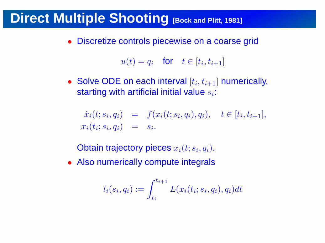
Direct Multiple Shooting [Bock and Plitt, 1981]
• Discretize controls piecewise on a coarse grid
u(t) = qi for t ∈ [ti, ti+1]
• Solve ODE on each interval [ti, ti+1] numerically,starting with artificial initial value si:
xi(t; si, qi) = f(xi(t; si, qi), qi), t ∈ [ti, ti+1],
xi(ti; si, qi) = si.
Obtain trajectory pieces xi(t; si, qi).
• Also numerically compute integrals
li(si, qi) :=
∫ ti+1
ti
L(xi(ti; si, qi), qi)dt

Sketch of Direct Multiple Shooting
r r r r r
6s0 s1
sisi+1
xi(ti+1; si, qi) 6= si+1
@@R
r r r r r
6
qix0 fr
-q
t0
q0q
t1
q q
ti
q
ti+1
q q
tN−1
r sN−1
q
tN
r sN

NLP in Direct Multiple Shooting
q q q q q q q q q q
6
bq
-p p p p p p p
q
p
q
minimizes, q
N−1∑
i=0
li(si, qi) + E (sN )
subject to
s0 − x0 = 0, (initial value)si+1 − xi(ti+1; si, qi) = 0, i = 0, . . . , N − 1, (continuity)
h(si, qi) ≥ 0, i = 0, . . . , N, (discretized path constraints)r (sN ) ≥ 0. (terminal constraints)
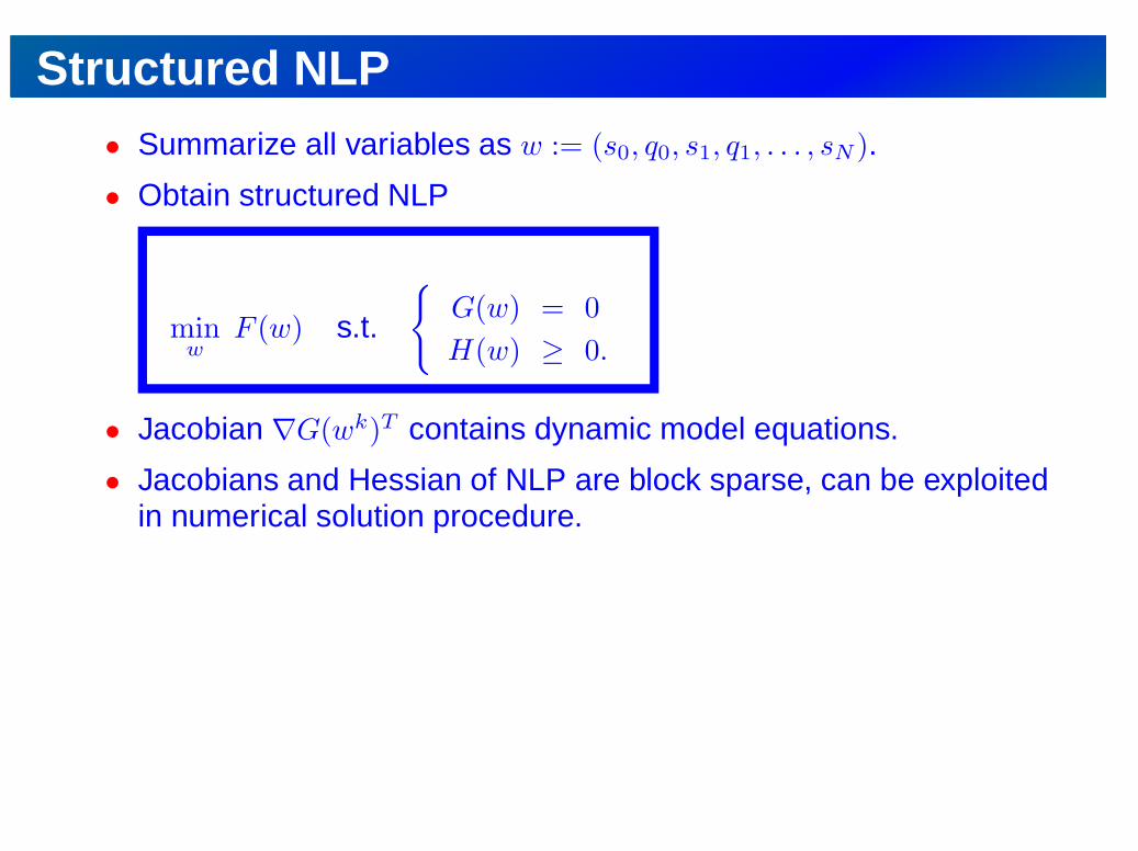
Structured NLP• Summarize all variables as w := (s0, q0, s1, q1, . . . , sN ).
• Obtain structured NLP
minw
F (w) s.t.
{
G(w) = 0
H(w) ≥ 0.
• Jacobian ∇G(wk)T contains dynamic model equations.
• Jacobians and Hessian of NLP are block sparse, can be exploitedin numerical solution procedure.

Test Example: Initialization with u(t) ≡ 0
single shooting:

Multiple Shooting: First Iteration
single shooting:

Multiple Shooting: 2nd Iteration
single shooting:
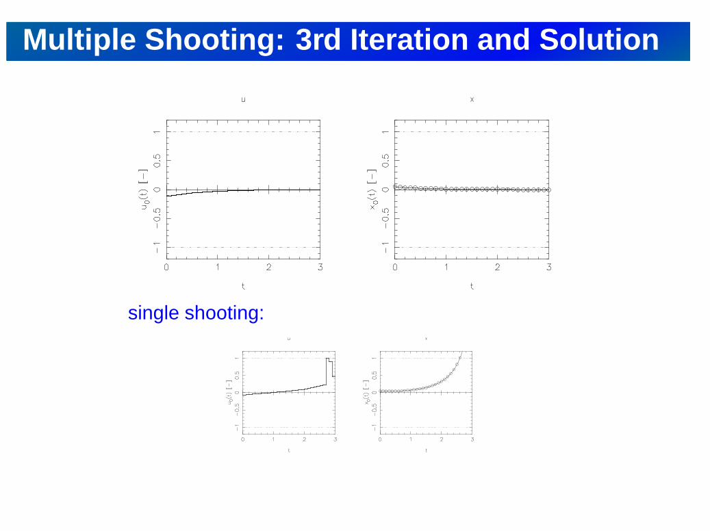
Multiple Shooting: 3rd Iteration and Solution
single shooting:

Direct Multiple Shooting: Pros and Cons
• Simultaneous simulation and optimization.
+ uses adaptive ODE/DAE solvers
+ but NLP has fixed dimensions
+ can use knowledge of x in initialization (here bounds; moreimportant in online context).
+ can treat unstable systems well.
+ robust handling of path and terminal constraints.
+ easy to parallelize.
- not as sparse as collocation.
• Used for practical optimal control e.g by Franke (“HQP”), Terwen(DaimlerChrysler); Santos and Biegler; Bock et al. (“MUSCOD-II”)

Conclusions: Optimal Control Family Tree(((((((((((((((((((
����������
��
��
Hamilton-Jacobi-Bellman Equation:
Tabulation inState Space
Indirect Methods,Pontryagin:
Solve Boundary ValueProblem
Direct Methods:Transform into Nonlinear
Program (NLP)
(((((((((((((((((((
����������
��
��
Single Shooting:Only discretized controls
in NLP(sequential)
Collocation:Discretized controls and
states in NLP(simultaneous)
Multiple Shooting:Controls and node start
values in NLP(simultaneous/hybrid)

Literature• T. Binder, L. Blank, H. G. Bock, R. Bulirsch, W. Dahmen, M. Diehl, T.
Kronseder, W. Marquardt and J. P. Schler, and O. v. Stryk:Introduction to Model Based Optimization of Chemical Processes onMoving Horizons. In Grötschel, Krumke, Rambau (eds.): OnlineOptimization of Large Scale Systems: State of the Art, Springer, 2001.pp. 295–340.
• John T. Betts: Practical Methods for Optimal Control Using NonlinearProgramming. SIAM, Philadelphia, 2001. ISBN 0-89871-488-5
• Dimitri P. Bertsekas: Dynamic Programming and Optimal Control.Athena Scientific, Belmont, 2000 (Vol I, ISBN: 1-886529-09-4) & 2001(Vol II, ISBN: 1-886529-27-2)
• A. E. Bryson and Y. C. Ho: Applied Optimal Control, Hemisphere/Wiley,1975.