More infinity for a better finitism

HAL Id: hal-00670733https://hal.archives-ouvertes.fr/hal-00670733

Submitted on 16 Feb 2012

HAL is a multi-disciplinary open accessarchive for the deposit and dissemination of sci-entific research documents, whether they are pub-lished or not. The documents may come fromteaching and research institutions in France orabroad, or from public or private research centers.

L’archive ouverte pluridisciplinaire HAL, estdestinée au dépôt et à la diffusion de documentsscientifiques de niveau recherche, publiés ou non,émanant des établissements d’enseignement et derecherche français ou étrangers, des laboratoirespublics ou privés.

More infinity for a better finitismSam Sanders

To cite this version:Sam Sanders. More infinity for a better finitism. Annals of Pure and Applied Logic, Elsevier Masson,2010, 161 (12), pp.1525. 10.1016/j.apal.2010.06.003. hal-00670733

https://hal.archives-ouvertes.fr/hal-00670733

https://hal.archives-ouvertes.fr

MORE INFINITY FOR A BETTER FINITISM

SAM SANDERS

Abstract. Elementary Recursive Nonstandard Analysis, in short ERNA, is

a constructive system of nonstandard analysis with a PRA consistency proof,proposed around 1995 by Patrick Suppes and Richard Sommer. It is based on

an earlier system developed by Rolando Chuaqui and Patrick Suppes. Here,

we discuss the inherent problems and limitations of the classical nonstandardframework and propose a much-needed refinement of ERNA, called ERNAA,

in the spirit of Karel Hrbacek’s stratified set theory. We study the meta-

mathematics of ERNAA and its extensions. In particular, we consider severaltransfer principles, both classical and ‘stratified’, which turn out to be related.

Finally, we show that the resulting theory allows for a truly general, elegant

and elementary treatment of basic analysis.

1. Introduction

By now, it is well-known that large parts of ‘ordinary’ mathematics can bedeveloped in systems much weaker than ZFC ([20], [21]). However, most theoriesunder consideration are at least as strong as WKL0, which is conservative over IΣ1.It is usually mentioned (see e.g. [1], [2] and [20]) that it should be possible to developa large part of mathematics in much weaker systems, in particular in I∆0 + expand related systems. Most notably, there is Friedman’s Grand Conjecture (see [2]and [6]):

Every theorem published in the Annals of Mathematics whose state-ment involves only finitary mathematical objects (i.e. what logicianscall an arithmetical statement) can be proved in EFA.

In 1929, Jacques Herbrand already made a similar claim, but without specifyingthe underlying logical system (see [9, p152]).

In this way, there have been attempts at developing analysis in nonstandardversions of I∆0 + exp (see [1], [4], [12], [23], [24] and [25]). In particular, the theoryERNA and its predecessor NQA+ (see [12] and [17]) are such systems. Accordingto Chuaqui, Sommer and Suppes, the latter theories ‘provide a foundation that isclose to mathematical practice characteristic of theoretical physics’. In order toachieve this goal, the systems satisfy the following three conditions, listed in [4]:

(i) The formulation of the axioms is essentially a free-variable one with no useof quantifiers.

(ii) We use infinitesimals in an elementary way drawn from nonstandard anal-ysis, but the account here is axiomatically self-contained and deliberatelyelementary in spirit.

(iii) Theorems are left only in approximate form; that is, strict equalities andinequalities are replaced by approximate equalities and inequalities. In

University of Ghent, Department of Pure Mathematics and Computer Algebra,

Galglaan 2, B-9000 Gent (Belgium)Telephone/Fax: +3292648573 / +3292644993E-mail address: [email protected].

2000 Mathematics Subject Classification. 03H15, 26E35.Key words and phrases. Relative, stratified, nonstandard, quantifier-free, analysis, ERNA.

1

2 MORE INFINITY FOR A BETTER FINITISM

particular, we use neither the notion of standard function nor the standardpart function.

It is also mentioned in [4], that another standard practice of physics, namely theuse of physically intuitive but mathematically unsound reasoning, is not reflectedin the system.

By limiting the strength of the systems according to (i)-(iii), the consistency ofERNA can be proved in PRA, using Herbrand’s theorem in the following form (see[4] and [23]).

1. Theorem (Herbrand). A quantier-free theory T is consistent if and only if everyfinite set of instantiated axioms of T is consistent.

In this respect, the item (i) is not merely a technicality to suit Herbrand’s the-orem: the quantifier-free axioms reflect the absence of existential quantifiers inphysics. As all ε-δ definitions of basic analysis are equivalent to universal nonstan-dard formulas, it indeed seems plausible that one can develop calculus inside ERNAand NQA+ in a quantifier-free way, particularly, without the use of ε-δ-statements.However, we discuss two compelling arguments why such a development is impos-sible.

First, as exemplified by item (iii), NQA+ has no ‘standard part’ function ‘st’,which maps every finite number x to the unique standard number y such thatx ≈ y. Thus, nonstandard objects like integrals and derivatives are only defined‘up to infinitesimals’. This leads to problems when trying to prove e.g. the fun-damental theorems of calculus, which express that differentiation and integrationcancel each other out. Indeed, in [4, Theorem 8.3], Chuaqui and Suppes prove thefirst fundamental theorem of calculus, using the previously proved corollary 7.4.The latter states that differentiation and integration cancel each other out on thecondition that the mesh du of the hyperfinite Riemann sum of the integral and theinfinitesimal y used in the derivative satisfy du/y ≈ 0. Thus, for every y, there is adu such that for all meshes dv ≤ du the corresponding integral and derivative can-cel each other out. The definition of the Riemann integral ([4, Axiom 18]) absorbsthis problem, but the former is quite complicated as a consequence. Also, it doesnot change the fact that ε-δ-statements occur, be it swept under the proverbialnonstandard carpet. Similary, ERNA only proves a version of Peano’s existencetheorem with a condition similar to du/y ≈ 0, contrary to Sommer and Suppes’claim in [24] (see [18]). Thus, ERNA and NQA+ cannot develop basic analysiswithout invoking ε-δ statements.

Second, we consider to what extent classical nonstandard analysis is actuallyfree of ε-δ-statements. For all functions in the standard language, the well-knownclassical ε-δ definitions of continuity or Riemann integrability, which are Π3, canbe replaced by universal nonstandard formulas (see e.g. [22, p70]). Given thateven most mathematicians find it difficult to work with a formula with more thantwo quantifier alternations, this is a great virtue. Indeed, using the nonstandardmethod greatly reduces the sometimes tedious ‘epsilon management’ when workingwith several ε-δ statements, see [27]. Yet, nonstandard analysis is not completelyfree of ε-δ statements. For instance, consider the function δ(x) = 1

πε

ε2+x2 , with

ε ≈ 0 and let f(x) be a standard C∞ function with compact support. Calculatingthe (nonstandard) Riemann integral of δ(x) × f(x) yields f(0). Hence δ(x) is anonstandard version of the Dirac Delta. However, not every Riemann sum withinfinitesimal mesh is infinitely close to the Riemann integral: the mesh has to besmall enough (compared to ε). Moreover, δ(x) ≈ δ(y) is not true for all x ≈ y, onlyfor x and y close enough. In general, most functions which are not in the standard

MORE INFINITY FOR A BETTER FINITISM 3

language do not have an elegant universal definition of continuity or integrabilityand we have to resort to ε-δ statements. Thus, nonstandard analysis only partiallyremoves the ε-δ formalism.

These two arguments show that the ‘regular’ nonstandard framework does notallow us to develop basic analysis in a quantifier-free way in weak theories of arith-metic. Moreover, for treating more advanced analysis, like the Dirac Delta, preva-lent in physics, we would have to resort to ε-δ-statements anyway. Inspired byHrbacek’s ‘stratified analysis’ (see [10] and [11]), we introduce a weak theory of

arithmetic, called ERNAA, which will allow us to develop analysis in a quantifier-free way. To this end, the theory ERNAA has a multitude of sets of infinite numbersinstead of the usual dichotomy of one set of finite numbers O, complemented withone set of infinite numbers Ω. Indeed, in ERNAA there is a linear ordering (A,)with least number 0, such that for all nonzero α, β ∈ A, the infinite number ωαis finite compared to ωβ for β α. Hence there are many ‘degrees’ or ‘levels’ ofinfinity and the least number 0 in the ordering (A,) corresponds to the standardlevel. It should be noted that the first nonstandard set theory involving differentlevels of infinity was introduced by Peraire in [16]. Another approach was developedby Gordon in [7].

In the second section, we describe ERNAA and its fundamental features andin the third section, we prove the consistency of ERNAA inside PRA. Thoughimportant in its own right, in particular for ‘strict’ finitism (see [26]), we not only

wish to do quantifier-free analysis in ERNAA, but also study its metamathematics.Thus, in the fourth section, we introduce the ‘Stratified Transfer Principle’, whichexpresses that a true formula should hold at all levels (see [10]). As ERNAA isa weak theory of arithmetic, we limit ourselves to transfer for universal formulas.This will turn out to be sufficient for developing analysis. Stratified Transfer equallyapplies to external formulas and is thus very different from transfer principles inregular nonstandard arithmetic. In the fifth section, we introduce various transferprinciples for ERNAA, which are based on transfer principles for ERNA (see [12]and [13]). It turns out that these ‘regular’ transfer principles imply the StratifiedTransfer Principle, which is remarkable, given the fundamental difference in scopebetween both. In the sixth section, we prove several important theorems of analysisin ERNAA and extensions. In the last section, we argue that Stratified Transferyields a good formal framework for theoretical physics.

2. ERNAA, the system

In this section, we describe ERNAA and some of its fundamental features.

2.1. The language. Let (A,) be a fixed linear order with least element 0, e.g.(N,≤) or (Q+,≤). For brevity, we write ‘α ≺ β’ instead of ‘α β ∧ α 6= β’.

2. Definition. The language L of ERNAA includes ERNA’s, minus the symbols‘ω’, ‘ε’ and ‘≈’. Additionally, it contains, for every nonzero α ∈ A, two constants‘ωα’ and ‘εα’ and, for every α ∈ A, a binary predicate ‘≈α’.

The set A and the predicate are not part of the language of ERNAA. However,we shall sometimes informally refer to them in theorems and definitions. Note thatthere are no constants ω0 and ε0 in L.

3. Definition. For all α ∈ A, the formula ‘x ≈α 0’ is read ‘x is α-infinitesimal’,‘x is α-infinite’ stands for ‘x 6= 0 ∧ 1/x ≈α 0’; ‘x is α-finite’ stands for ‘x is notα-infinite’; ‘x is α-natural’ stands for ‘x is hypernatural and α-finite’.


4. Definition. If L is the language of ERNAA, then Lα-st, the α-standard languageof ERNAA, is L without ≈β for all β ∈ A and without ωβ and εβ for β α.

For α = 0, we usually drop the addition ‘0’. For instance, we write ‘natural’instead of ‘0-natural’ and ‘≈’ instead of ‘≈0’. Note that in this way, L0-st is Lst,the standard language of ERNAA.

5. Definition. A term or formula is called internal if it does not involve ≈α forany α ∈ A; if it does, it is called external.

2.2. The axioms. The axioms of ERNAA include ERNA’s, minus axiom 7.(4) (Hy-pernaturals), axiom set 11 (Infinitesimals) and axiom set 37 (External minimum).

Additionally, ERNAA contains the following axiom set.

6. Axiom set (Infinitesimals).

(1) If x and y are α-infinitesimal, so are x+ y and x× y.(2) If x is α-infinitesimal and y is α-finite, xy is α-infinitesimal.(3) An α-infinitesimal is α-finite.(4) If x is α-infinitesimal and |y| ≤ x, then y is α-infinitesimal.(5) If x and y are α-finite, then so is x+ y.(6) The number εα is β-infinitesimal for all β ≺ α.(7) The number ωα = 1/εα is hypernatural and α-finite.

7. Theorem. The number ωα is β-infinite for all β ≺ α.

Proof. Immediate from items (6) and (7) of the previous axiom set.

8. Theorem. x is α-finite iff there is an α-natural n such that |x| ≤ n.

Proof. The statement is trivial for x = 0. If x 6= 0 is α-finite, so is |x| because,assuming the opposite, 1/|x| would be α-infinitesimal and so would 1/x be byaxiom 6.(4). By axiom 6.(5), the hypernatural n = d|x|e < |x| + 1 is then alsoα-finite. Conversely, let n be α-natural and |x| ≤ n. If 1/|x| were α-infinitesimal,so would 1/n be by axiom 6.(4), and this contradicts the assumption that n isα-finite.

Thus, we see that Lα-st is just Lst with all α-finite constants added.

9. Corollary. x ≈α 0 iff |x| < 1/n for all α-natural n ≥ 1.

For completeness, we list ERNA’s ‘weight’ axioms and the related theorems, aswe will repeatedly use them.

10. Axiom set (Weight).

(1) if ‖x‖ is defined, then ‖x‖ is a nonzero hypernatural.(2) if |x| = m/n ≤ 1 (m and n 6= 0 hypernaturals), then ‖x‖ is defined, ‖x‖.|x|

is hypernatural and ‖x‖ ≤ n(3) if |x| = m/n ≥ 1 (m and n 6= 0 hypernaturals), then ‖x‖ is defined, ‖x‖/|x|

is hypernatural and ‖x‖ ≤ m.

11. Theorem.

(1) If x is not a hyperrational, then ‖x‖ is undefined.(2) If x = ±p/q with p and q 6= 0 relatively prime hypernaturals, then

‖ ± p/q‖ = max|p|, |q|.

12. Theorem.

(1) ‖0‖ = 1(2) if n ≥ 1 is hypernatural, ‖n‖ = n(3) if ‖x‖ is defined, then ‖1/x‖ = ‖x‖ and ‖ dxe ‖ ≤ ‖x‖


(4) if ‖x‖ and ‖y‖ are defined, ‖x+ y‖, ‖x− y‖, ‖xy‖ and ‖x/y‖ are at mostequal to (1 + ‖x‖)(1 + ‖y‖), and ‖x y‖ is at most (1 + ‖x‖) (1 + ‖y‖).

13. Notation. For any 0 < n ∈ N we write ‖(x1, . . . , xn)‖ = max‖x1‖, . . . , ‖xn‖.

3. The consistency of ERNAA

In this section, we prove the consistency of ERNAA inside PRA. We need thedetails of this proof for the proof of theorem 21.

As ERNAA is a quantifier-free theory, we can use Herbrand’s theorem in thesame way as in [12], [13] and [23], for more details, see [3] or [8]. To obtain ERNA’soriginal consistency proof from the following, omit ≈α for α 6= 0 from the language.

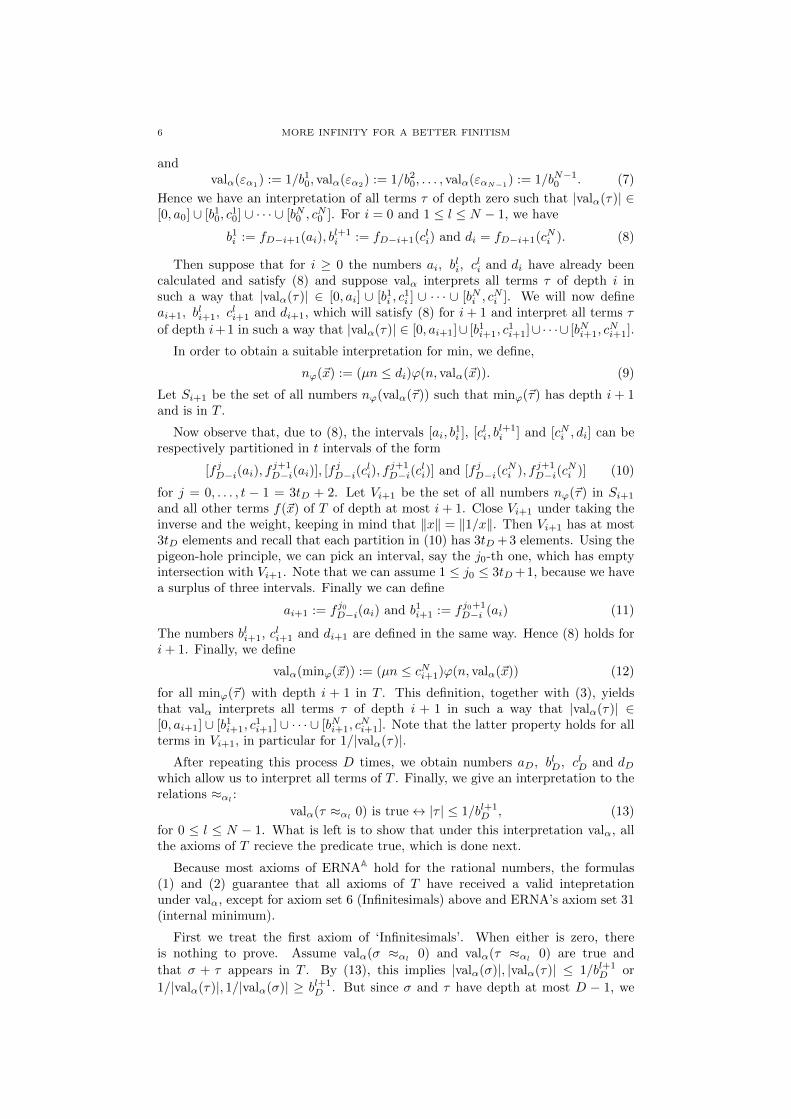
14. Theorem. The theory ERNAA is consistent and this consistency can be provedin PRA.

Proof. In view of Herbrand’s theorem, it suffices to show the consistency of everyfinite set of instantiated axioms of ERNAA. Let T be such a set. We will definea mapping valα on T , similar to the mapping val in ERNA’s consistency proof.Thus, valα maps the terms of T to rationals and the relations of T to relationson rationials, in such a way that all axioms of T are true under valα. Hence T isconsistent and the theorem follows.

First of all, as there are only finitely many elements of A in T , we interpret(A,) as a suitable initial segment of (N,≤).

Second, like in the consistency proof of ERNA, all standard terms of T , exceptfor min, are interpreted as their homomorphic image in the rationals: for all termsoccurring in T , except min, εα, ωα, we define

valα(f(x1, . . . , xk)) := f(valα(x1), . . . , valα(xk)) (1)

and for all relations R occurring in T , except ≈α, we define

valα(R(x1, . . . , xk)) is true↔ R(valα(x1), . . . , valα(xk)). (2)

Third, we need to gather some technical machinery. Let D be the maximumdepth of the terms in T and let α0, α1, α2, . . . , αN−1 be all numbers of A that

occur in T , with α0 = 0. As ERNAA has the same axiom schema for recursion asERNA, no standard term of ERNAA grows faster than 2xk, for k ∈ N. Hence, by[12, Theorem 30], there is a 0 < B ∈ N such that for every term f(~x) occurring inT , not involving min, we have

||f(~x)|| ≤ 2||~x||B . (3)

Further assume that tD is the number of terms of depth D one can create usingonly function symbols occurring in T , and define t := 3tD + 3.With t and D, define the following functions:

f0(x) = 2xB and fn+1(x) = f tn(x) = fn(fn(. . . (fn(x))))︸︷︷︸t fn’s

. (4)

Furthermore, define a0 := 1 and

b10 := fD+1(a0), c10 := b10, b20 := fD+1(c10), c20 := b20, . . . , b

N0 := fD+1

(cN−10

), (5)

and finally cN0 := bN0 and d0 := fD+1(cN0 ).

The numbers bl0 allow us to interpret εα and ωα:

valα(ωα1) := b10, valα(ωα2) := b20, . . . , valα(ωαN−1) := bN−10 (6)


andvalα(εα1) := 1/b10, valα(εα2) := 1/b20, . . . , valα(εαN−1

) := 1/bN−10 . (7)

Hence we have an interpretation of all terms τ of depth zero such that |valα(τ)| ∈[0, a0] ∪ [b10, c

10] ∪ · · · ∪ [bN0 , c

N0 ]. For i = 0 and 1 ≤ l ≤ N − 1, we have

b1i := fD−i+1(ai), bl+1i := fD−i+1(cli) and di = fD−i+1(cNi ). (8)

Then suppose that for i ≥ 0 the numbers ai, bli, c

li and di have already been

calculated and satisfy (8) and suppose valα interprets all terms τ of depth i insuch a way that |valα(τ)| ∈ [0, ai] ∪ [b1i , c

1i ] ∪ · · · ∪ [bNi , c

Ni ]. We will now define

ai+1, bli+1, c

li+1 and di+1, which will satisfy (8) for i+ 1 and interpret all terms τ

of depth i+1 in such a way that |valα(τ)| ∈ [0, ai+1]∪ [b1i+1, c1i+1]∪· · ·∪ [bNi+1, c

Ni+1].

In order to obtain a suitable interpretation for min, we define,

nϕ(~x) := (µn ≤ di)ϕ(n, valα(~x)). (9)

Let Si+1 be the set of all numbers nϕ(valα(~τ)) such that minϕ(~τ) has depth i + 1and is in T .

Now observe that, due to (8), the intervals [ai, b1i ], [cli, b

l+1i ] and [cNi , di] can be

respectively partitioned in t intervals of the form

[f jD−i(ai), fj+1D−i(ai)], [f

jD−i(c

li), f

j+1D−i(c

li)] and [f jD−i(c

Ni ), f j+1

D−i(cNi )] (10)

for j = 0, . . . , t − 1 = 3tD + 2. Let Vi+1 be the set of all numbers nϕ(~τ) in Si+1

and all other terms f(~x) of T of depth at most i+ 1. Close Vi+1 under taking theinverse and the weight, keeping in mind that ‖x‖ = ‖1/x‖. Then Vi+1 has at most3tD elements and recall that each partition in (10) has 3tD + 3 elements. Using thepigeon-hole principle, we can pick an interval, say the j0-th one, which has emptyintersection with Vi+1. Note that we can assume 1 ≤ j0 ≤ 3tD+1, because we havea surplus of three intervals. Finally we can define

ai+1 := f j0D−i(ai) and b1i+1 := f j0+1D−i (ai) (11)

The numbers bli+1, cli+1 and di+1 are defined in the same way. Hence (8) holds fori+ 1. Finally, we define

valα(minϕ(~x)) := (µn ≤ cNi+1)ϕ(n, valα(~x)) (12)

for all minϕ(~τ) with depth i + 1 in T . This definition, together with (3), yieldsthat valα interprets all terms τ of depth i + 1 in such a way that |valα(τ)| ∈[0, ai+1] ∪ [b1i+1, c

1i+1] ∪ · · · ∪ [bNi+1, c

Ni+1]. Note that the latter property holds for all

terms in Vi+1, in particular for 1/|valα(τ)|.After repeating this process D times, we obtain numbers aD, b

lD, c

lD and dD

which allow us to interpret all terms of T . Finally, we give an interpretation to therelations ≈αl :

valα(τ ≈αl 0) is true↔ |τ | ≤ 1/bl+1D , (13)

for 0 ≤ l ≤ N − 1. What is left is to show that under this interpretation valα, allthe axioms of T recieve the predicate true, which is done next.

Because most axioms of ERNAA hold for the rational numbers, the formulas(1) and (2) guarantee that all axioms of T have received a valid intepretationunder valα, except for axiom set 6 (Infinitesimals) above and ERNA’s axiom set 31(internal minimum).

First we treat the first axiom of ‘Infinitesimals’. When either is zero, thereis nothing to prove. Assume valα(σ ≈αl 0) and valα(τ ≈αl 0) are true and

that σ + τ appears in T . By (13), this implies |valα(σ)|, |valα(τ)| ≤ 1/bl+1D or

1/|valα(τ)|, 1/|valα(σ)| ≥ bl+1D . But since σ and τ have depth at most D − 1, we


have 1/|valα(τ)|, 1/|valα(σ)| ∈ [0, aD−1]∪ [b1D−1, c1D−1]∪· · ·∪ [bND−1, c

ND−1] and since

aD−1 ≤ aD ≤ bl+1D ≤ bl+1

D−1, they must be in ∪l+1≤k≤N [bkD−1, ckD−1]. Hence we

have 1/|valα(τ)|, 1/|valα(σ)| ≥ bl+1D−1 or |valα(τ)|, |valα(σ)| ≤ 1/bl+1

D−1, from which

|valα(σ + τ)| ≤ 2/bl+1D−1 < 1/bl+1

D . This last inequality is true, since bl+1D > 2 and

(bl+1D )2 < bl+1

D−1. We have proved that |valα(σ + τ)| ≤ 1/bl+1D , which is equivalent

to valα(σ + τ ≈αl 0) being true. Hence the first axiom of the set ‘Infinitesimals’receives the predicate true under valα.

The second axiom of ‘Infinitesimals’ is treated in the same way as the first one.

The third axiom of ‘Infinitesimals’ holds trivially under val, since we cannot havethat |valα(τ)| ≤ 1/bl+1

D and 1/|valα(τ)| ≤ 1/bl+1D hold at the same time. The fact

that zero is αl-finite, is immediate by the definition of the predicate ‘x is αl-finite’.

The fourth axiom of ‘Infinitesimals’ holds trivially, thanks to (13).

The fifth axiom of ‘Infinitesimals’ is treated like the first and second axiom ofthe same set.

The sixth and seventh item of ‘Infinitesimals’ both follow from (6), (7) and (13).

Now we will treat the axioms of the schema ‘internal minimum’. First, note thatthe interval [cNi+1, d

Ni+1], defined as in (11), has empty intersection with Vi+1. In

particular, no term nϕ(~τ) of T ends up in this interval. Thus, for terms minϕ ofdepth i+ 1, we have

valα(minϕ(~τ)) = (µn ≤ cNi+1)ϕ(n, valα(~τ)) = (µn ≤ cND)ϕ(n, valα(~~τ)) (14)

as cND is in the interval [cNi+1, dNi+1]. We are ready to consider items (1)-(3) of

the internal minimum schema. It is clear that item (1) always holds. For item(2), assume that the antecedent holds, i.e. valα(minϕ(~τ) > 0) is true. By thedefinition of valα(minϕ) in (12), the consequent ϕ(valα(minϕ(~τ)), valα(~τ)) holdstoo. Hence item (2) holds. For item (3), assume that the antecedent holds, i.e.ϕ(valα(σ), valα(~τ)) holds for some σ in T . This implies valα(σ) ≤ cND and thusthere is a number n ≤ cND such that ϕ(n, valα(~τ)). By (14), valα(minϕ(~τ)) is theleast of these and hence the formulas ‘minϕ(~τ) ≤ σ’ and ‘ϕ(minϕ(~τ), ~τ)’ receive atrue interpretation under valα. Thus, item (3) is also interpreted as true and weare done with this schema.

All axioms of T have received a true interpretation under valα, hence T is consis-tent and, by Herbrand’s theorem, ERNAA is. Now, Herbrand’s theorem is provablein IΣ1 and this theory is Π2-conservative over PRA (see [3, 8]). As consistencycan be formalized by a Π1-formula, it follows immediately that PRA proves theconsistency of ERNAA.

Note that if we define, in (5), a0 as a number larger than 1 and any cl0 as anumber larger than bl0, we still obtain a valid interpretation valα for T and theconsistency proof goes through.

The choice of (A,) is arbitrary, hence it is consistent with ERNAA that A is

dense. It is possible to make this explicit by adding the following axiom to ERNAA,for all nonzero α, β ∈ A.

ωα < ωβ → ωα < ωα+β2

< ωβ . (15)

The notation ‘α+β2 ’ is of course purely symbolic. This axiom receives a valid inter-pretation by interpreting (A,) as (Q,≤).

In the following, we repeatedly need overflow and underflow. Thus, we prove itexplicitly in ERNAA.


15. Theorem. Let ϕ(n) be an internal quantifier-free formula, not involving min.

(1) If ϕ(n) holds for every α-natural n, it holds for all hypernatural n up tosome α-infinite hypernatural n (overflow).

(2) If ϕ(n) holds for every α-infinite hypernatural n, it holds for all hypernaturaln from some α-natural n on (underflow).

Both numbers n and n are given by explicit ERNAA-formulas not involving min.

Proof. Let ω be some α-infinite number. For the first item, define

n := (µn ≤ ω)¬ϕ(n+ 1), (16)

if (∃n ≤ ω)¬ϕ(n+ 1) and zero otherwise. By theorem [12, Theorem 58], this term

is available in ERNA and hence in ERNAA. Likewise for underflow.

The previous theorem shows that overflow holds for all α ∈ A, i.e. at all levelsof infinity. As no one level is given exceptional status, this seems only natural.Furthermore, one intuitively expects formulas that do not explicitly depend on acertain level to be true at all levels if they are true at one. In the following section,we investigate a general principle that transfers universal formulas to all levels ofinfinity.

4. ERNAA and Stratified Transfer

In nonstandard mathematics, Transfer expresses Leibniz’s principle that the‘same’ laws hold for standard and nonstandard objects alike. Typically, Trans-fer only applies to formulas involving standard objects, excluding e.g. ERNA’s

cosine∑ωi=0(−1)i x

2i

(2i)! . In set theoretical approaches to nonstandard analysis, the

standard part function ‘st’ applied to such an object, results in a standard object,thus solving this problem. The latter function is not available in ERNA, but ‘gen-eralized’ transfer principles for objects like ERNA’s cosine can be obtained (see[13, Theorem 19] and [18]), at the cost of introducing ‘≈’. Unfortunately, formulaswith occurrences of the predicate ‘≈’ are always excluded from Transfer, even inthe classical set-theoretical approach.

For ERNAA, we wish to obtain a transfer principle that applies to all universalformulas, possibly involving ≈. As an example, consider the following formula,expressing the continuity of the standard function f on [0, 1]:

(∀x, y ∈ [0, 1])(x ≈ y → f(x) ≈ f(y)). (17)

Assuming (17), it seems only natural that if x ≈α y for α 0, then f(x) ≈α f(y).In other words, there should hold, for all α ∈ A,

(∀x, y ∈ [0, 1])(x ≈α y → f(x) ≈α f(y)), (18)

which is (17), with ≈ replaced with ≈α. Incidentally, when f is a polynomial,an easy computation shows that (18) indeed holds, even for polynomials in Lα-st.Below, we turn this into a general principle.

16. Notation. Let Φα be a formula of Lα-st ∪ ≈α. Then Φβ is Φα with alloccurrences of ≈α replaced with ≈β .

17. Principle (Stratified Transfer). Assume α 0 and let Φα be a quantifier-freeformula of Lα-st ∪ ≈α, not involving min. For every β α,

(∀~x)Φα(~x)↔ (∀~x)Φβ(~x). (19)

Note that Φ may involve α-standard parameters. We always tacitly allow (α-standard) parameters in all transfer principles in this paper, unless explicitly statedotherwise.


18. Principle (Weak Stratified Transfer). Assume α 0 and let f(~x, k) be afunction of Lα-st, not involving min and weakly increasing in k. For all β α, thefollowing statements are equivalent

‘f(~x, k) is α-infinite for all ~x and all α-infinite k’

and

‘f(~x, k) is β-infinite for all ~x and all β-infinite number k’.

The second transfer principle is a special case of the first. However, by thefollowing theorem, the seemingly weaker second principle is actually equivalent tothe first. We sometimes abbreviate ‘for all α-infinite ω’ by ‘(∀αω)’.

19. Theorem. In ERNAA, Weak Stratified Transfer is equivalent to StratifiedTransfer.

Proof. First, assume the Weak Stratified Transfer Principle and let Φα(~x) be asin the Stratified Transfer Principle. Replace in Φα(~x) all positive occurrences ofτi(~x) ≈α 0 with (∀α-stni)(|τi(~x)| < 1/ni), where ni is a new variable not yet ap-pearing in Φα(~x). Do the same for the negative occurrences, using new variablesmi. Bringing all quantifiers in (∀~x)Φα(~x) to the front, we obtain

(∀~x)(∀α-stn1, . . . , nl)(∃α-stm1, . . . ,mk)Ψ(~x, n1, . . . , nl,m1, . . . ,mk),

where Ψ is quantifier-free and in Lα-st. Using pairing functions, we can reduceall ni to one variable n and reduce all mi to one variable m. Hence the previousformula becomes

(∀~x)(∀α-stn)(∃α-stm)Ξ(~x, n,m),

where Ξ is quantifier-free and in Lα-st. Fix some α-infinite number ω1, we obtain

(∀~x)(∀α-stn)(∃m ≤ ω1)Ξ(~x, n,m),

Applying overflow, with ω = ω1 in (16), yields

(∀~x)(∀n ≤ n(~x, ω1))(∃m ≤ ω1)Ξ(~x, n,m).

Hence the function n(~x, k) is α-infinite for all ~x and α-infinite k and weakly increas-ing in k. By the Weak Stratified Transfer Principle, n(~x, k) is β-infinite for all ~xand all β-infinite k, for β α. Hence, for all ~x, β-finite n and β-infinite k, we have

(∃m ≤ k)Ξ(~x, n,m).

Fix ~x0 and β-finite n0. Since (∃m ≤ k)Ξ(~x0, n0,m) holds for all β-infinite k,underflow yields (∃β-stm)Ξ(~x0, n0,m). This implies

(∀~x)(∀β-stn)(∃β-stm)Ξ(~x, n,m).

Unpairing the variables n and m and bringing the quantifiers back in the formula,we obtain (∀~x)Φβ(~x). Thus, we have proved the forward implication in (19).

In the same way, it is proved that (∀~x)Φβ(~x) implies (∀~x)Φα(~x), i.e., the reverseimplication in (19), assuming the Weak Stratified Transfer Principle.

Hence we proved that the Weak Stratified Transfer Principle implies the Strati-fied Transfer Principle. As the reverse implication is trivial, we are done.

By the previous theorem, it suffices to prove the consistency of ERNAA with theWeak Stratified Transfer Principle. Instead of proving this consistency directly, weshow, in the next section, that Weak Stratified Transfer follows from Πα

3 -TRANS.

The latter is ERNAA’s version of the classical transfer principle limited to Π3-formulas. The schema Πα

3 -TRANS is analogous to Π1-TRANS and Σ2-TRANS,introduced in [12] and [13]. We suspect that PRA cannot prove the consistency of

ERNAA + Πα3 -TRANS.


To conclude this section, we point to [10], where the importance of Stratified

Transfer is discussed. Moreover, analysis developed in ERNAA in section 6 is moreelegant when Stratified Transfer is available. Also, Stratified Transfer (in someform or other) seems to be compatible with the spirit of ‘strict’ finitism (see [26]),as it merely lifts true universal formulas to higher levels. It would be interesting toknow the exact logical strength of Stratified Transfer and how it can be weakenedby imposing certain ‘constructive’ limitations on A.

5. ERNAA and regular Transfer

In this section, we will introduce the ‘new’ transfer principles Πα1 -TRANS and

Σα2 -TRANS, which are ERNAA-versions of the ‘old’ schemas Π1-TRANS and Σ2-TRANS. The adaptations made to the latter schemas to obtain the former areboth natural and in line with the Stratified Transfer Principle above. We give aconsistency proof for the extended theory, which requires significant changes to theconsistency proof in [12]. We only sketch a consistency proof for ERNAA + Σα2 -TRANS. Finally, using the new transfer principles, we prove that transfer for Π3-formulas is sufficient for the Stratified Transfer Principle.

5.1. Transfer for Π1 and Σ1-formulas. Here, we introduce a ‘stratified’ versionof transfer for Π1 and Σ1-formulas for ERNAA and show that the extended theoryis consistent. The following axiom schema is ERNAA’s version of Π1-TRANS.

20. Axiom schema (Stratified Π1-transfer). For every quantifier-free formula ϕ(n)of Lα-st, not involving min, we have

(∀α-stn)ϕ(n)→ (∀n)ϕ(n). (20)

The previous axiom schema is denoted by Πα1 -TRANS and its parameter-free

counterpart is denoted by Πα1 -TRANS−. Similarly, let Π1-TRANS− be the parameter-

free version of Π1-TRANS (see also remark 52). After the consistency proof, thereasons for the restrictions on ϕ will become apparent. Resolving the implicationin (20), we see that this formula is equivalent to

(0 < min¬ϕ is α-finite) ∨ (∀n)ϕ(n). (21)

Thus, ERNAA + Πα1 -TRANS− is equivalent to a quantifier-free theory and we may

use Herbrand’s theorem to prove its consistency. To obtain the consistency proofin [12] from the following proof, omit ≈α for α 6= 0 from the language.

21. Theorem. The theory ERNAA + Πα1 -TRANS− is consistent and this consis-

tency can be proved by a finite iteration of ERNAA’s consistency proof.

Proof. Despite the obvious similarities between the theories ERNA + Π1-TRANS−

and ERNAA + Πα1 -TRANS−, the consistency proof of the former (see [12, Theorem

44]) breaks down for the latter. The reason is that one of the explicit conditions forthe consistency proof of ERNA + Π1-TRANS− to work, is that ϕ must be in Lst.But in Πα

1 -TRANS−, ϕ is in Lα-st and as such, the formula ϕ in (21) may containthe nonstandard number ωβ for β α.

However, it is possible to salvage the original proof. We use Herbrand’s theoremin the same way as in the consistency proof of ERNAA. Thus, let T be any finite setof instantiated axioms of ERNAA + Πα

1 -TRANS−. Leaving out the transfer axioms

from T , we are left with a finite set T ′ of instantiated ERNAA axioms. Let valαbe its interpretation into the rationals as in ERNAA’s consistency proof. However,nothing guarantees that the instances of Πα

1 -TRANS− in T are also interpreted as‘true’ under valα. We will adapt valα by successively increasing the starting values


defined in (5), if necessary. The resulting map will interpret all axioms in T as true,not just those in T ′.

Let T and T ′ be as in the previous paragraph. Let D be the maximum depthof the terms in T . Let α0, . . . , αN−1 be all elements of A in T , with α0 = 0. Fornotational convenience, for ϕ as in Πα

1 -TRANS−, we shall write ϕ(n, ~τ) instead ofϕ(n), where ~τ contains all numbers occurring in ϕ that are not in Lst. Finally,let the list ϕ1(n, ~τ1), . . . , ϕM (n, ~τM ) consist of the quantifier-free formulas whoseΠα

1 -transfer axiom (21) occurs in T . If necessary, we arrange this list of formulasin such a way that i < j implies that all ωα in the range of ~τi satisfy ωα ωβ forsome ωβ in the range of ~τj .

By (13), Ωl :=⋃l+1≤i≤N [biD, c

iD] is the set where valα maps the αl-infinite

numbers. Also, Ol := [0, aD] ∪ [b1D, c1D] ∪ · · · ∪ [blD, c

lD] is the set where valα maps

the αl-finite numbers. If we have, for all i ∈ 1, ...,M and all l ∈ 0, ..., N − 1such that γ αl for all ωγ in the range of ~τi, that

(∃m ∈ Ol)¬ϕi(m, valα(~τi)) ∨ (∀n ∈ [0, aD] ∪ Ω0)ϕi(n, valα(~τi)), (22)

we see that valα provides a true interpretation of the whole of T , not just T ′, asevery instance of (21) receives a valid interpretation, in this case. However, nothingguarantees that (22) holds for all such numbers i and l. Thus, assume there is anexceptional ϕ′(n, ~τ ′) := ϕi(n, ~τi) and l, for which

(∀m ∈ Ol)ϕ′(m, valα(~τ ′)) ∧(∃n ∈

[bl+1D , cl+1

D

])¬ϕ′(n, valα(~τ ′)). (23)

Now fix ~τ ′ and let l0 be the least l satisfying the previous formula. Then (23) implies(∃n ∈ Ωl0)¬ϕ′(n, val(~τ ′)), i.e. there is an ‘αl0 -infinite’ n such that ¬ϕ′(n, val(~τ ′)).Now choose a number n0 > cND (for notational clarity, we write a0 = c00, for thecase l0 = 0) and construct a new interpretation val′α with the same starting values

as in (5), except for (cl00 )′ := n0. This val′α continues to make the axioms in T ′ trueand does the same with the instances in T of the axiom

(0 < min¬ϕ′(~τ′) is αl0-finite) ∨ (∀n)ϕ′(n, ~τ ′) (24)

Indeed, if a number n ∈ Ωl0 is such that ¬ϕ′(n, valα(~τ ′)), the number n is inter-

preted by val′α as an αl0-finite number because n ≤ cND ≤ (cl00 )′ ≤ (cl0D)′ by our

choice of (cl00 )′. Thus, the sentence (∃n ∈ O′l0)¬ϕ′(n, valα(~τ ′)) is true. By defini-

tion, ~τ ′ only contains numbers ωαi for i ≤ l0 and (6) implies valα(ωαi) = bi0, for

1 ≤ i ≤ N . But increasing cl00 to (cl00 )′, as we did before, does not change the num-

bers b10,. . . , bl00 . Hence valα(~τ ′) = val′α(~τ ′) and so (∃n ∈ O′l0)¬ϕ′(n, valα(~τ ′)) implies

(∃n ∈ O′l0)¬ϕ′(n, val′α(~τ ′)). Thus, (0 < min¬ϕ′(~τ′) is αl0-finite) is true under val′α

and so is the whole of (24).

Define T ′′ as T ′ plus all instances of (24) occurring in T . If there is anotherexceptional ϕi and l0 such that (23) holds, repeat this process. Note that if we

increase another cj0 for j ≥ l0 and construct val′′α, the latter still makes the axioms

of T ′ true, but the axioms of T ′′ as well, since increasing cj0 does not change theinterpretations of the numbers ωαi for i ≤ l0 either. Hence (24) is true underval′′ for the same reason as for val′. Recall that the list ϕ1(n, ~τ1), . . . , ϕM (n, ~τM )is arranged in such a way that i < j implies that all ωα in the range of ~τi satisfyωα ωβ for some ωβ in the range of ~τj . This arrangement of the list guarantees thatthe changes we make to valα to satisfy a certain transfer axiom, do not invalidatea transfer axiom treated earlier.

This process, repeated, will certainly halt: either the two lists 1, . . . ,M and1, . . . , N − 1 become exhausted or, at some earlier stage, a valid interpretation is

found for T . Note that this consistency proof is a finite iteration of ERNAA’s.


The restrictions on the formulas ϕ admitted in (20) are imposed by our consis-tency proof. Indeed, for every αi occurring in T , the interpretation of ωαj for j > i

depends on the choice of ci0. By our changing cl00 into (cl00 )′ > cl00 , formulas like(24) could loose their ‘true’ interpretation from one step to the next, if they containsuch ωj . Likewise, the changing of cl0 can change the interpretation of ≈β , for anyβ ∈ A, and hence this predicate cannot occur in ϕ. The exclusion of min has, ofcourse, a different reason: minϕ is only allowed in ERNA when ϕ does not rely onmin.

For convenience, we will usually use Πα1 -TRANS instead of Πα

1 -TRANS−. Bycontraposition, the schema Πα

1 -TRANS implies the following schema, which wedenote Σα1 -TRANS.

22. Axiom schema (Stratified Σ1-transfer). For every quantifier-free formula ϕ(n)of Lα-st, not involving min, we have

(∃n)ϕ(n)→ (∃α-stn)ϕ(n). (25)

Note that both in (20) and (25), the reverse implication is trivial. For ϕ ∈ Lα-st,the levels β α are sometimes called the ‘context’ levels of ϕ and α is the calledthe ‘minimial’ context level, i.e. the lowest level on which all constants occurringin ϕ exist. In this respect, Σα1 -transfer expresses that true existential formulas canbe pushed down to their minimal context level, which corresponds to their level ofstandardness.

5.2. Transfer for Σ2 and Π2-formulas. In order to obtain transfer for Σ2 andΠ2-formulas in ERNA, we added a certain axiom schema to ERNA + Π1-TRANSand showed that the resulting theory has transfer for Σ2 and Π2-formulas, see [13]for details. We also discussed why this approach is preferable to a more ‘direct’approach. Here, we shall employ the same method to obtain ‘Stratified Transfer’for Σ2 and Π2-formulas. As the method is similar to that used in [13], we onlysketch the proofs. Our goal is to obtain the following transfer principle.

23. Axiom schema (Stratified Σ2-transfer). For every quantifier-free formula ϕfrom Lα-st, not involving min, we have

(∃n)(∀m)ϕ(n,m)↔ (∃α-stn)(∀α-stm)ϕ(n,m). (26)

We denote this schema by Σα2 -TRANS. By contraposition, it is equivalent to theΠα

2 -transfer principle

(∀n)(∃m)ϕ(n,m)↔ (∀α-stn)(∃α-stm)ϕ(n,m). (27)

In view of the equivalence between (26) and (27), we will only mention Πα2 -transfer

in the sequel if it is explicitly required. We will add certain axioms to ERNAA +Πα

1 -TRANS and prove the consistency of the resulting theory. Then we show thatthe extended theory proves the above Σα2 -transfer principle.

First consider the following theorem of ERNAA + Πα1 -TRANS.

24. Theorem. In ERNAA +Πα1 -TRANS we have, for every quantifier-free formula

ϕ(n,m) of Lα-st not involving min, the implication

(∃n)(∀m)ϕ(n,m)→ (∀α-stk)(∃α-stn)(∀m ≤ k)ϕ(n,m). (28)

Proof. If the antecedent holds, we have (∃n)(∀m ≤ k)ϕ(n,m) for every α-finite k.By Σα1 -transfer, (∃α-stn)(∀m ≤ k)ϕ(n,m), hence the consequent of (28).

By the previous theorem, (29) implies the forward implication in (26).


25. Axiom schema (TRANS+α ). For every quantifier-free formula ϕ(n,m) of Lα-st

not involving min, we have

(∃n)(∀m)ϕ(n,m)→

(∀α-stk)(∃α-stn)(∀m ≤ k)ϕ(n,m)↓

(∃α-stn)(∀α-stm)ϕ(n,m)

(29)

Theorem 27 will show that Σα2 -transfer as stated in (26) is provable in ERNAA +

Πα1 -TRANS+TRANS+

α . Therefore, the latter theory will be abbreviated to ERNAA+Σα2 -TRANS. The schema TRANS+

α can be skolemized in exactly the same way asthe schema TRANS+, see [13, Theorem 3] for details. We have the following theo-rem.

26. Theorem. The theory ERNAA + Σα2 -TRANS is consistent.

Proof. The proof of the consistency of ERNA + Σ2-TRANS in [13] can easily beconverted into a proof for the theorem at hand. The adaptations are minimal, asthe skolemization of (29) is also a tautology in the finite setting of the model for

an arbitrary finite subset of instantiated ERNAA + Πα1 -TRANS-axioms.

Now we prove the main result of this section, viz. that ERNAA + Σα2 -TRANShas Σα2 -transfer.

27. Theorem. In ERNAA + Σα2 -TRANS, the Σα2 -transfer principle, stated in (26),holds.

Proof. By theorem 26 we know that we can consistently add the axiom schema 25to ERNAA + Πα

1 -TRANS. In the extended theory, theorem 24 yields that (29)implies the forward implication in (26). For the inverse implication, assume that(∃α-stn)(∀α-stm)ϕ(n,m) and fix α-finite n0 such that (∀α-stm)ϕ(n0,m). By Πα

1 -transfer, this implies (∀m)ϕ(n0,m) and hence (∃n)(∀m)ϕ(n,m).

Using pairing functions, we immediately obtain Stratified Σα2 and Πα2 -transfer

for formulas involving blocks of quantifiers. As for Σα1 -transfer, Σα2 -transfer as in(26) expresses that a true Σ2-formula can be pushed down to its minimal contextlevel

5.3. Transfer for Σ3 and Π3-formulas. Here, we show that a certain transferprinciple for Π3-formulas, called Πα

3 -TRANS, is sufficient to obtain Weak StratifiedTransfer. We first introduce the former. Note that it is the natural extension ofΣα2 and Πα

1 -transfer.

28. Axiom schema (Stratified Π3-transfer). For every quantifier-free formula ϕof Lα-st, not involving min, we have,

(∀α-stn)(∃α-stm)(∀α-stk)ϕ(n,m, k)↔ (∀n)(∃m)(∀k)ϕ(n,m, k). (30)

We denote this schema by Πα3 -TRANS. We now prove the main theorem of this

section, namely that Πα3 -transfer is sufficient to obtain Stratified Transfer.

29. Theorem. The theory ERNAA+Πα3 -TRANS proves the Weak Stratified Trans-

fer Principle.

Proof. Assume 0 α ≺ β and let f be as in the Weak Stratified Transfer Principleand assume that f(n, ~x) is α-infinite for all ~x and all α-infinite n. This implies that

(∀~x)(∀α-stn)(∀αω)(f(ω, ~x) > n),

where the notation ‘(∀αω)’ denotes ‘for all α-infinite numbers ω’. Fixing ~x0 andα-finite n0 and applying underflow to the formula (∀αω)(f(ω, ~x0) > n0), yields theexistence of an α-finite number k0 such that (f(k0, ~x0) > n0). Hence,

(∀~x)(∀α-stn)(∃α-stm)(f(m,~x) > n), (31)


and, by [12, Theorem 58], there is a function g(n, ~x) which calculates the least msuch that f(m,~x) > n, for any ~x and α-finite n. Thus, (31) implies

(∀α-stn)(∀~x)(f(g(n, ~x), ~x) > n), (32)

where g(n, ~x) is α-finite for α-finite n and any ~x. Now fix an α-infinite hypernaturalω1 and define h(n) as max‖~x‖≤ω1

g(n, ~x). By definition, the function h(n) is α-finitefor α-finite n. As f is weakly increasing in its first argument, (32) implies

(∀α-stn)(∀~x)(‖~x‖ ≤ ω1 → f(h(n), ~x) > n),

and also

(∀α-stn)(∃m ≤ h(n))(∀~x)(‖~x‖ ≤ ω1 → f(m,~x) > n).

We previously showed that h(n) is α-finite for α-finite n. Thus,

(∀α-stn)(∃α-stm)(∀~x)(‖~x‖ ≤ ω1 → f(m,~x) > n),

and also

(∀α-stn)(∃α-stm)(∀α-st~x)(f(m,~x) > n). (33)

By Πα3 -transfer, this implies that

(∀β-stn)(∃β-stm)(∀β-st~x)(f(m,~x) > n). (34)

Fixing appropriate β-finite n0 and m0, and applying Πα1 -transfer, yields

(∀β-stn)(∃β-stm)(∀~x)(f(m,~x) > n).

This formula implies that f(k, ~x) is β-infinite for all ~x and all β-infinite k. Theother implication in the Weak Stratified Transfer Principle is proved in the sameway.

It is clear form the proof why the theorem fails for β such that 0 β ≺ α.Indeed, as f may contain ωα, we cannot apply Πα

3 -transfer to (33) for such β.

Note that (Weak) Stratified Transfer is fundamentally different from the othertransfer principles, as ≈α can occur in the former, but not in the latter. In thisrespect, it is surprising that a ‘regular’ transfer principle such as Πα

3 -TRANS implies(Weak) Stratified Transfer.

However, if we consider things from the point of view of set theory, we canexplain this remarkable correspondence between ‘regular’ and ‘stratified’ transfer.Internal set theory is an axiomatic approach to nonstandard mathematics (see [14]for details). Examples include Nelson’s IST ([15]), Kanovei’s BST ([14]), Peraire’sRIST ([16]) and Hrbacek’s FRIST∗ and GRIST ([10] and [11]), which inspired

parts of ERNAA. These set theories are extensions of ZFC and most have a so called‘Reduction Algorithm’. This effective procedure applies to certain general classesof formulas and removes any predicate not in the original ∈-language of ZFC. Theresulting formula agrees with the original formula on standard objects. Thus, inGRIST, it is possible to remove the relative standardness predicate ‘v’ and hencetransfer for formulas in the ∈-v-language follows from transfer for formulas in the∈-language. Similarly, in theorem 19, we show that transfer for formulas involvingthe relative standardness predicate ≈α can be reduced to a very specific instance,involving fewer predicates ≈α. Later, in theorem 29, we prove that the remainingstandardness predicates can be removed from the formula too, producing (33) and(34). Thus, we have reduced ‘stratified’ transfer to ‘regular’ transfer. In turn, itis surprising that a set-theoretical metatheorem such as the Reduction Algorithmappears in theories with strength far below ZFC.


6. Analysis in ERNAA

In this section, we obtain some basic theorems of analysis. We shall work inERNAA + Πα

3 -TRANS, i.e. we may use the Stratified Transfer Principle. Most

theorems can be proved in ERNAA, at the cost of adding extra technical conditions.This is usually mentioned in a corollary.

For the rest of this section, we assume that 0 ≺ α ≺ β, that a and b are α-finiteand that the functions f and g do not involve the minimum operator minϕ.

6.1. Continuity. Here, we define the notion of continuity in ERNAA and provesome fundamental theorems.

30. Definition. A function f is α-continuous at a point x0, if x ≈α x0 impliesf(x) ≈α f(x0). A function is α-continuous over [a, b] if

(∀x, y ∈ [a, b])(x ≈α y → f(x) ≈α f(y)).

As usual, we write ‘continuous’ instead of ‘0-continuous’. If f is α and β-continuous for α 6= β, we say that f is ‘α, β-continuous’

31. Theorem. If f is α-continuous over [a, b] and α-finite in one point of [a, b], itis α-finite for all x in [a, b].

Proof. Let f be as in the theorem, fix α-finite k0 and consider

(∀x, y ∈ [a, b])(|x− y| ≤ 1/N ∧ ‖x, y‖ ≤ ωβ → |f(x)− f(y)| < 1/k0). (35)

As f is α-continuous, this formula holds for all α-infinite N . By [12, Corollary 53],(35) is quantifier-free and applying underflow yields that it holds for all N ≥ N0,where N0 is α-finite. Then let x0 ∈ [a, b] be such that f(x0) is α-finite. Wemay assume it satisfies ‖x0‖ ≤ ωβ . Using (35) for N = N0, it easily follows thatf(x) deviates at most (N0db − ae)/k0 from f(x0) for ‖x‖ ≤ ωβ . As the points

xn := a + n(b−a)ωβ

partition the interval [a, b] in α-infinitesimal subintervals, the

theorem follows.

32. Corollary. If f ∈ Lα-st is α-continuous over [a, b], it is α-finite for all x ∈ [a, b].

Proof. Let f(x, ~x) be the function f(x) from the corollary with all nonstandardnumbers replaced with free variables. By [12, Theorem 30], there is a k ∈ N such

that ‖f(x, ~x)‖ ≤ 2‖x,~x‖k . Thus, f(x) is α-finite for α-finite x. Applying the theorem

finishes the proof.

By Stratified Transfer, an α-continuous function of Lα-st(e.g. ERNAA’s cosine∑ωα

n=0(−1)n x2n

(2n)!

)is also β-continuous for all β α. Similar statements hold for

integrability and differentiability. For the sake of brevity, we mostly do not explicitlymention these properties.

6.2. Differentiation. Here, we define the notion of differentiability in ERNAA andprove some fundamental theorems. To this end, we need some notation.

33. Notation.

(1) A nonzero number x is ‘α-infinitesimal’ or ‘strict α-infinitesimal’ (with re-spect to β) if x ≈α 0 ∧ x 6≈β 0. We denote this by x ≈α 0.

(2) We write ‘a α b’ instead of ‘a < b ∧ a 6≈α b’ and ‘a /βb’ instead of

‘a < b ∨ a ≈β b’.(3) We write ∆h(f)(x) instead of f(x+h)−f(x)

h .

We use the following notion of differentiability.


34. Definition.

(1) A function f is ‘α-differentiable at x0’ if ∆εf(x0) ≈α ∆ε′f(x0) for allnonzero ε, ε′ ≈α 0 and both quotients are α-finite.

(2) If f is α-differentiable at x0 and ε ≈α 0, then ∆εf(x0) is called ‘the deriv-ative of f at x0’ and is denoted Dαf(x0).

(3) A function f is called ‘α-differentiable over (a, b)’ if it is α-differentiable atevery point aα xα b.

(4) The concepts ‘α-differentiable’ and ‘α-derivative’ are defined by replacing,in the previous items, ‘ε, ε′ ≈α 0’ by ‘ε, ε′ ≈α 0’. We use the same notationfor the α-derivative as for the α-derivative.

The choice of ε is arbitrary and hence the derivative is only defined ‘up toinfinitesimals’. There seems to be no good way of defining it more ‘precisely’, i.e.not up to infinitesimals, without the presence of a ‘standard part’ function ‘stα’which maps α-finite numbers to their α-standard part.

35. Theorem. If a function f is α-differentiable over (a, b), it is α-continuous atall aα xα b.

Proof. Immediate from the definition of differentiability.

36. Theorem. Let f(x) and g(x) be α-standard and α-differentiable over (a, b).Then f(x)g(x) is α-differentiable over (a, b) and

Dα(fg)(x) ≈α Dαf(x) g(x) + f(x)Dαg(x) (36)

for all aα xα b.

Proof. Assume f and g are α-differentiable over (a, b). Let ε be an α-infinitesimaland x such that aα xα b. Then,

Dα(fg)(x) ≈α 1ε (f(x+ ε)g(x+ ε)− f(x)g(x))

= 1ε (f(x+ ε)g(x+ ε)− f(x)g(x+ ε) + f(x)g(x+ ε)− f(x)g(x))

= 1ε ((f(x+ ε)− f(x))g(x+ ε) + f(x)(g(x+ ε)− g(x)))

= f(x+ε)−f(x)ε g(x+ ε) + f(x) g(x+ε)−g(x)ε

≈α Dαf(x)g(x+ ε) + f(x)Dαg(x) ≈α Dαf(x)g(x) + f(x)Dαg(x).

The final two steps follow from theorem 35 and corollary 32. Hence f(x)g(x) isα-differentiable over (a, b) and (36) indeed holds.

By theorem 31, the requirement ‘f, g ∈ Lα-st’ in the previous theorem, can bedropped if we additionally require fg to be α-finite in one point of (a, b). In thefollowing theorem, there is no such requirement.

37. Theorem (Chain rule). Let g be α-differentiable at a and let f be α-differentiableat g(a). Then f g is α-differentiable at a and

Dα(f g)(a) ≈α Dαf(g(a))Dαg(a). (37)

Proof. Let f and g be as in the theorem and assume 0 6= ε ≈α 0. First of all, since

g is α-differentiable at a, we have, that Dαg(a) ≈α g(a+ε)−g(a)ε , which implies

g(a+ ε) = εDαg(a) + g(a) + εε′

for some ε′ ≈α 0. Then ε′′ = εDαg(a) + εε′ is also α-infinitesimal. If ε′′ 6= 0, then,

as f is α-differentiable at g(a), we have Dαf(g(a)) ≈α f(g(a)+ε′′)−f(g(a))ε′′ . This

implies

f(g(a) + ε′′) = ε′′Dαf(g(a)) + f(g(a)) + ε′′ε′′′


for some ε′′′ ≈α 0. If ε′′ = 0, then the previous formula holds trivially for the same

ε′′′. Note that ε′′ε′′′

ε ≈α 0. Hence we have

∆ε(f g)(a) = f(g(a+ε))−f(g(a))ε = f(g(a)+ε′′)−f(g(a))

ε

= ε′′Dαf(g(a))+ε′′ε′′′+f(g(a))−f(g(a))ε ≈α ε′′

ε Dαf(g(a)).

By definition, ε′′

ε ≈α Dαg(a) and hence f g is α-differentiable at a and (37)holds.

It is easily verified that the theorems of this section still hold if we replace ‘α-differentiable’ with ‘α-differentiable’.

6.3. Integration. Here, we define the notion of Riemann integral in ERNAA andprove some fundamental theorems.

In classical analysis, the Riemann-integral is defined as the limit of Riemannsums over ever finer partitions. In ERNAA, we adopt the following definition forthe concept ‘partition’.

38. Definition. A partition π of [a, b] is a vector (x1, . . . , xn, t1, . . . tn−1) such thatxi ≤ ti ≤ xi+1 for all 1 ≤ i ≤ n − 1 and a = x1 and b = xn. The numberδ = max2≤i≤n(xi − xi−1) is called the ‘mesh’ of the partition π.

For the definition of integrability, we need to quantify over all partitions of aninterval. In [12], it is proved that ERNA contains pairing functions, which canuniquely code vectors of numbers into numbers (and decode them back). As par-titions are merely vectors, it is intuitively clear that quantifying over all partitionsof an interval is possible in ERNA, and thus in ERNAA. Also, in [18], the previ-ous claim is proved explicitly. Incidentally, Riemann integration inside NQA+, thepredecessor of ERNA, uses equidistant partitions.

Assume that ω is α-infinite and that a α b. Let n0 be the least n such thatnω > a and let n1 be the least n such that n

ω > b. Define aω := n0

ω and bω := n1−1ω .

Like the derivative, the Riemann integral can only be defined ‘up to infinitesimals’.Hence, for α-Riemann integrable functions, it does not matter whether we use theinterval [a, b] or the interval [aω, bω] in its definition. From now on, we tacitlyassume that aα b.

39. Definition (Riemann Integration). Let f be a function defined on [a, b].

(1) Given a partition (x1, . . . , xn, t1, . . . , tn−1) of [a, b], the Riemann sum cor-responding to f is defined as

∑ni=2 f(ti−1)(xi − xi−1).

(2) The function f is α-Riemann integrable on [a, b], if for all partitions of [a, b]with mesh ≈α 0, the Riemann sums are α-finite and α-infinitely close.

(3) If f is α-Riemann integrable on [a, b], then the integral of f over [a, b],

denoted as∫ baf(x) d(x, α), is the Riemann sum corresponding to f of the

equidistant partition of [aω, bω] with mesh ε = 1ω ≈α 0 and points ti =

xi+1+xi2 .

40. Theorem. A function f which is α-continuous and α-finite over [a, b], is α-Riemann integrable over [a, b].

Proof. The proof for α = 0 is given in [18] and can easily be adapted to α 0.

41. Theorem. Let f be α-continuous and α-finite over [a, b] and assume a α

cα b. Hence,∫ baf(x) d(x, α) ≈α

∫ caf(x) d(x, α) +

∫ bcf(x) d(x, α).


Proof. Immediate from the previous theorem and the definition of the Riemannintegral.

42. Theorem. Let c be an α-finite positive constant such that c 6≈α 0 and let f beα-continuous and α-finite over [a, b+ c]. We have∫ b

af(x+ c) d(x, α) ≈α

∫ b+ca+c

f(x) d(x, α).

Proof. Immediate from theorem 40 and the definition of the Riemann integral.

43. Theorem (Second fundamental theorem). Let f ∈ Lα-st be α-continuous on[a, b] and let F (x) be

∫ xaf(t)d(t, β). Then F (x) is α-differentiable over (a, b) and

the equation DαF (x) ≈α f(x) holds for all aα xα b.

Proof. Fix ε ≈α 0 and x such that aα xα b. We have

F (x+ε)−F (x)ε = 1

ε

(∫ x+εa

f(t)d(t, β)−∫ xaf(t)d(t, β)

)≈β 1

ε

∫ x+εx

f(t)d(t, β), (38)

as ε is not β-infinitesimal. Let ω1 be β-infinite and define xi = x + iεω1

. Let f(y1)

and f(y2) be the least and the largest f(xi) for i ≤ ω1. As f is α,β-continuous,m := f(y1) and M := f(y2) are such that m /

βf(y) /

βM for y ∈ [x, x + ε] and

m ≈α M ≈α f(x). This implies

εm /β

∫ x+εx

f(t)d(t, β) /βεM,

and hencem /

β

1ε

∫ x+εx

f(t)d(t, β) /βM,

as ε is not β-infinitesimal. Thus,

m ≈α 1ε

∫ x+εx

f(t)d(t, β) ≈α M ≈α f(x).

By (38), F is α-differentiable and the theorem follows.

44. Corollary. The condition ‘f ∈ Lα-st’ in the theorem can be dropped if werequire f to be α, β-continuous over [a, b] and α-finite in one point of [a, b].

Proof. It is an easy verification that the proof of the theorem still goes throughwith these conditions.

45. Example. Define ε = ε4α. The function d(x) = εε2+x2 is α, β-continuous for

α-finite x and at most 1/ε4α. The function arctanx :=∫ x0d(t,β)1+t2 is α-differentiable

in all α-finite x and we have Dα

(arctan(x/ε)

)≈α ε

ε2+x2 for all α-finite x.

46. Theorem (First fundamental theorem). Let f ∈ Lα-st be α-differentiable over(a, b) and such that Dαf is β-continuous over [a, b]. For a α c α d α b, we

have∫ dcDαf(x) d(x, β) ≈α f(d)− f(c).

Proof. Let c, d be as stated and let ε be strict α-infinitesimal. Note that d − c isα-finite. We have∫ d

cDαf(x) d(x, β) ≈α

∫ dcf(x+ε)−f(x)

ε d(x, β)

≈β 1ε

(∫ dcf(x+ ε) d(x, β)−

∫ dcf(x) d(x, β)

)≈β 1

ε

(∫ d+εc+ε

f(x) d(x, β)−∫ dcf(x) d(x, β)

)≈β 1

ε

(∫ d+εd

f(x) d(x, β)−∫ c+εc

f(x) d(x, β)).

As in the proof of the second fundamental theorem, we have∫ c+εc

f(x) d(x, β) ≈αf(c) and

∫ d+εd

f(x) d(x, β) ≈α f(d) and we are done.


47. Corollary (Partial Integration). Let f, g ∈ Lα-st be α-differentiable over (a, b)and let Dαf and Dαg be β-continuous over [a, b]. For aα cα dα b,∫ d

c

f(x)Dαg(x) d(x, β) ≈α[f(x)g(x)

]dc−∫ d

c

Dαf(x)g(x) d(x, β).

Proof. Immediate from the second fundamental theorem and theorem 36.

By theorem 35, we can drop the requirement ‘f, g ∈ Lα-st’ if we additionallyrequire fg to be α-finite in one point of (a, b).

For simulating the Dirac Delta distribution, we need to introduce an extra levelγ such that 0 ≺ γ ≺ α. We also need the function arctan.

48. Theorem. Define the (finite) constant π as 4 arctan(1).

(1) For all α-finite x, arctan(±|x|) + arctan(± 1|x|)≈α ±π/2.

(2) We have arctan(±ω3α) ≈γ ±π/2.

Proof. The first item follows by calculating the α-derivative of arctanx+arctan 1/xusing the chain rule and noting that the result is α-infinitesimally close to zero.Thus, there is a constant C such that arctanx + arctan 1/x ≈α C, for all α-finitepositive x. Substituting x = 1 yields C = π/2. The case x < 0 is treated inthe same way. The second item follows from the previous item and the fact thatarctanx is γ-continuous at zero.

49. Definition. A function f ∈ Lγ-st is said to have a ‘compact support’ if it iszero outside some interval [a, b] with a, b γ-finite.

50. Theorem. Let f ∈ Lγ-st be an γ-differentiable function with compact supportsuch that Dαf(x) is β-continuous for x ≈γ 0. We have

1

π

ωα∫−ωα

d(x)f(x)d(x, β) ≈γ f(0).

Proof. Assume that f(x) is zero outside [a, b], with a, b γ-finite. First, we prove

that∫ bεαf(x)d(x) d(x, β) ≈γ 0. As |x| ≥ εα implies x2 ≥ ε2α we have d(x) =

εε2+x2 ≤ ε

x2 ≤ εεα2 = ε2α < εα. Hence the integral

∫ bεα|d(x)| |f(x)| d(x, β) is at

most εα∫ bεα|f(x)| d(x, β). As f is γ-finite and γ-continuous on [a, b], we have∫ b

εαf(x)d(x) d(x, β) ≈γ 0. In the same way, we have

∫ εαaf(x)d(x) d(x, β) ≈γ 0

and∫ εα−εα arctan(x/ε))Dαf(x) d(x, β) ≈γ 0. Hence we have

ωα∫−ωα

d(x)f(x)d(x, β) ≈β∫ b

a

d(x)f(x) d(x, β) ≈γ∫ εα

−εαd(x)f(x) d(x, β).

If 0 6∈ [a, b], then f(0) = 0 and the theorem follows. Otherwise, by example 45, thefunction d(x) is α-infinitesimally close to 1

πDα arctan(x/ε), yielding

εα∫−εα

d(x)f(x) d(x, β) ≈α1

π

εα∫−εα

Dα(arctan(x/ε)) f(x) d(x, β).


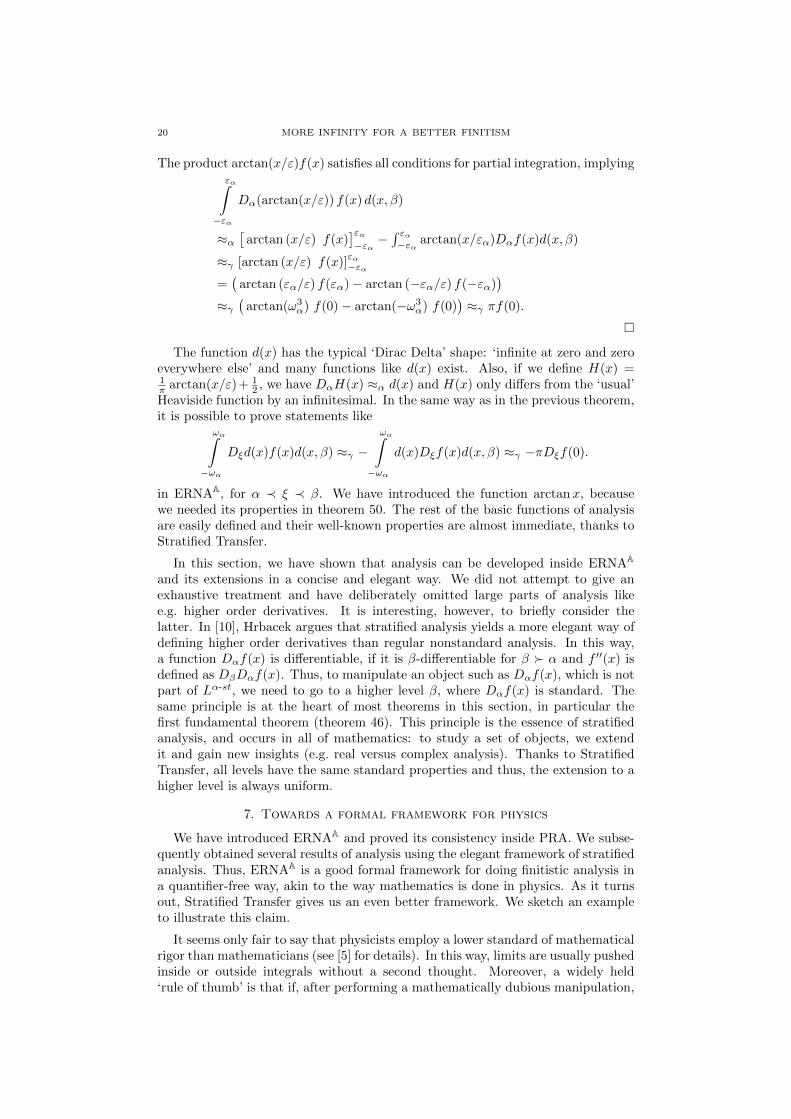
The product arctan(x/ε)f(x) satisfies all conditions for partial integration, implyingεα∫

−εα

Dα(arctan(x/ε)) f(x) d(x, β)

≈α[

arctan (x/ε) f(x)]εα−εα−∫ εα−εα arctan(x/εα)Dαf(x)d(x, β)

≈γ [arctan (x/ε) f(x)]εα−εα

=(

arctan (εα/ε) f(εα)− arctan (−εα/ε) f(−εα))

≈γ(

arctan(ω3α) f(0)− arctan(−ω3

α) f(0))≈γ πf(0).

The function d(x) has the typical ‘Dirac Delta’ shape: ‘infinite at zero and zeroeverywhere else’ and many functions like d(x) exist. Also, if we define H(x) =1π arctan(x/ε)+ 1

2 , we have DαH(x) ≈α d(x) and H(x) only differs from the ‘usual’Heaviside function by an infinitesimal. In the same way as in the previous theorem,it is possible to prove statements like

ωα∫−ωα

Dξd(x)f(x)d(x, β) ≈γ −ωα∫

−ωα

d(x)Dξf(x)d(x, β) ≈γ −πDξf(0).

in ERNAA, for α ≺ ξ ≺ β. We have introduced the function arctanx, becausewe needed its properties in theorem 50. The rest of the basic functions of analysisare easily defined and their well-known properties are almost immediate, thanks toStratified Transfer.

In this section, we have shown that analysis can be developed inside ERNAA

and its extensions in a concise and elegant way. We did not attempt to give anexhaustive treatment and have deliberately omitted large parts of analysis likee.g. higher order derivatives. It is interesting, however, to briefly consider thelatter. In [10], Hrbacek argues that stratified analysis yields a more elegant way ofdefining higher order derivatives than regular nonstandard analysis. In this way,a function Dαf(x) is differentiable, if it is β-differentiable for β α and f ′′(x) isdefined as DβDαf(x). Thus, to manipulate an object such as Dαf(x), which is notpart of Lα-st, we need to go to a higher level β, where Dαf(x) is standard. Thesame principle is at the heart of most theorems in this section, in particular thefirst fundamental theorem (theorem 46). This principle is the essence of stratifiedanalysis, and occurs in all of mathematics: to study a set of objects, we extendit and gain new insights (e.g. real versus complex analysis). Thanks to StratifiedTransfer, all levels have the same standard properties and thus, the extension to ahigher level is always uniform.

7. Towards a formal framework for physics

We have introduced ERNAA and proved its consistency inside PRA. We subse-quently obtained several results of analysis using the elegant framework of stratifiedanalysis. Thus, ERNAA is a good formal framework for doing finitistic analysis ina quantifier-free way, akin to the way mathematics is done in physics. As it turnsout, Stratified Transfer gives us an even better framework. We sketch an exampleto illustrate this claim.

It seems only fair to say that physicists employ a lower standard of mathematicalrigor than mathematicians (see [5] for details). In this way, limits are usually pushedinside or outside integrals without a second thought. Moreover, a widely held‘rule of thumb’ is that if, after performing a mathematically dubious manipulation,


the result still makes physical and (to a lesser extent) mathematical sense, themanipulation was probably sound. As it turns out, stratified nonstandard analysis isa suitable formal framework for this sort of ‘justification a posteriori’. We illustratethis with an example.

51. Example. Let fi, a and b be standard objects. According to the previouslymentioned ‘rule of thumb’, the following manipulation∫ b

a

∞∑i=0

fi(x, y) dx =

∞∑i=0

∫ b

a

fi(x, y) dx =:

∞∑i=0

gi(y) =: g(y)

is considered valid in physics as long as the function g(y) is physically and/or math-ematically meaningful. In stratified analysis, assuming 0 ≺ α ≺ β, the previousbecomes∫ b

a

ωα∑i=0

fi(x, y) d(x, β) ≈ωα∑i=0

∫ b

a

fi(x, y) d(x, β) =:

ωα∑i=0

hi(y) =: h(y).

The first step follows from Stratified Transfer. Indeed, as a finite summation can bepushed through a Riemann integral, a β-finite summation can be pushed througha β-Riemann integral. Thus, we can always obtain h(y) and if it is finite (the veryleast for it to be physically meaningful), we have h(y) ≈ g(y), thus justifying our‘rule of thumb’.

52. Remark. In [12], the authors introduce the transfer principle Π1-TRANS with-out stating whether standard parameters are allowed or not. Define Π1-TRANS(Π1-TRANS−) as schema 43 of [12] with (without) standard parameters in ϕ. Theproof of theorem 44 in [12] is obviously only correct for ERNA + Π1-TRANS−, asERNA + Π1-TRANS interprets IΣ1, by theorem 45 in the same paper. In the restof [12], in particular §4 and §6, the schema Π1-TRANS is used. The authors herebyapologize for this oversight. Although the schemas Πα

1 -TRANS− and Π1-TRANS−

originate from technical considerations, they turn out to play an important role inthe context of Reverse Mathematics. We will explore this avenue of research in [19].

53. Acknowledgement. The author thanks Professor Karel Hrbacek (City Uni-versity of New York, City College) for his valuable advice.

References

[1] Jeremy Avigad, Weak theories of nonstandard arithmetic and analysis, Reverse mathematics

2001, Lect. Notes Log., vol. 21, Assoc. Symbol. Logic, La Jolla, CA, 2005, pp. 19–46.[2] , Number theory and elementary arithmetic, Philos. Math. (3) 11 (2003), 257–284.

[3] Samuel R. Buss, An introduction to proof theory, Handbook of proof theory, Stud. Logic

Found. Math., vol. 137, North-Holland, Amsterdam, 1998, pp. 1–78.[4] Rolando Chuaqui and Patrick Suppes, Free-variable Axiomatic Foundations of Infinitesimal

Analysis: A Fragment with Finitary Consistency Proof, Journal of Symbolic Logic 60 (1995),

122-159.[5] Kevin Davey, Is mathematical rigor necessary in physics?, British J. Philos. Sci. 54 (2003),

no. 3, 439–463.[6] Harvey Friedman, Grand Conjectures, FOM mailing list (16 April 1999).

[7] E. I. Gordon, Nonstandard methods in commutative harmonic analysis, Vol. 164, American

Mathematical Society, Providence, RI, 1997.[8] Petr Hajek and Pavel Pudlak, Metamathematics of First-Order Aritmetic, Springer, 1998.

[9] Jacques Herbrand, Ecrits logiques, Presses Universitaires de France, Paris, 1968 (French).[10] Karel Hrbacek, Stratified analysis?, The strength of nonstandard analysis, Springer Wien,

New York, Vienna, 2007, pp. 47–63.

[11] , Relative set theory: internal view, J. Log. Anal. 1 (2009), Paper 8, 108.[12] Chris Impens and Sam Sanders, Transfer and a supremum principle for ERNA, Journal of

Symbolic Logic 73 (2008), 689-710.[13] , Saturation and Σ2-transfer for ERNA, J. Symbolic Logic 74 (2009), no. 3, 901–913.


[14] Vladimir Kanovei and Michael Reeken, Nonstandard analysis, axiomatically, Springer, 2004.

[15] Edward Nelson, Internal set theory: a new approach to nonstandard analysis, Bull. Amer.

Math. Soc. 83 (1977), no. 6, 1165–1198.[16] Yves Peraire, Theorie relative des ensembles internes, Osaka J. Math. 29 (1992), no. 2,

267–297 (French).[17] Michal Rossler and Emil Jerabek, Fragment of nonstandard analysis with a finitary consis-

tency proof, Bulletin of Symbolic Logic 13 (2007), 54-70.

[18] Sam Sanders, ERNA and Friedman’s Reverse Mathematics, To appear in Journal of SymbolicLogic.

[19] , Levels of Reverse Mathematics, In preparation.

[20] Stephen G. Simpson, Subsystems of second order arithmetic, Perspectives in MathematicalLogic, Springer-Verlag, Berlin, 1999.

[21] (ed.), Reverse mathematics 2001, Lecture Notes in Logic, vol. 21, Association for

Symbolic Logic, La Jolla, CA, 2005.[22] Keith D. Stroyan and Willem A.J. Luxemburg, Introduction to the theory of infinitesimals,

Academic Press, 1976.

[23] Richard Sommer and Patrick Suppes, Finite Models of Elementary Recursive NonstandardAnalysis, Notas de la Sociedad Matematica de Chile 15 (1996), 73-95.

[24] , Dispensing with the Continuum, Journal of Math. Psy. 41 (1997), 3-10.[25] Patrick Suppes and Rolando Chuaqui, A finitarily consistent free-variable positive fragment of

Infinitesimal Analysis, Proceedings of the IXth Latin American Symposium on Mathematical

Logic Notas de Logica Mathematica 38 (1993), 1-59.[26] Willem W. Tait, Finitism, The Journal of Philosophy 78 (1981), 524-564.

[27] Terence Tao, Ultrafilters, nonstandard analysis, and epsilon management, 2007. Wordpress

blog, http://terrytao.wordpress.com/.

More infinity for a better finitism

Documents

Transcript of More infinity for a better finitism