More Binding Pipelining - csl.cornell.edu · More resource sharing – Perfect graphs – Left-edge...
28
More Binding Pipelining ECE 5775 (Fall’17) High-Level Digital Design Automation
-
Upload
duonghuong -
Category
Documents
-
view
215 -
download
0
Transcript of More Binding Pipelining - csl.cornell.edu · More resource sharing – Perfect graphs – Left-edge...

More BindingPipelining
ECE 5775 (Fall’17)High-Level Digital Design Automation

▸ Lab 3 due Friday 10/6– No late penalty for this assignment (up to 3 days late)
▸ HW 2 will be posted tomorrow
1
Logistics
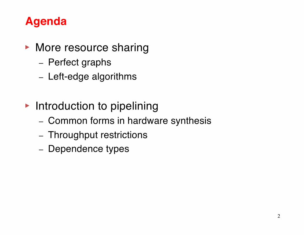
▸ More resource sharing– Perfect graphs – Left-edge algorithms
▸ Introduction to pipelining– Common forms in hardware synthesis– Throughput restrictions– Dependence types
2
Agenda

Review: Compatibility and Conflict Graphs
▸ Compatibility graph:– Partition the graph into a minimum number of cliques
• Clique in an undirected graph is a subset of its vertices such that every two vertices in the subset are connected by an edge
▸ Conflict graph:– Color the vertices by a minimum number of colors (chromatic
number), where adjacent vertices cannot use the same color
3
a b
c
d
a b
c
d
A scheduled DFG Clique partitioning on compatibility graph
a b
c
d
Coloring on conflict graph
Operations have same type

▸ Clique partitioning and graph coloring problems are NP-hard on general graphs, with the exception of perfect graphs
▸ Definition of perfect graphs– For every induced subgraph, the size of the maximum (largest)
clique equals the chromatic number of the subgraph– Examples: bipartite graphs, chordal graphs, etc.
• Chordal graphs: every cycle of four or more vertices has a chord, i.e., an edge between two vertices that are not consecutive in the cycle.
4
Perfect Graphs

▸ Intersection graphs of a (multi)set of intervals on a line – Vertices correspond to intervals– Edges correspond to interval intersection– A special class of chordal graphs
5
Interval Graph
[Figure source: en.wikipedia.org/wiki/Interval_graph]

Example: Meeting Scheduling
Meeting Schedule (am)A 9:00~11:00B 9:30~10:00C 10:00~11:00D 11:00~11:30
6
9:30 10:00 10:30 11:00 11:309:00
AB
CD
Gantt chart
Conflict graph chromatic number = 2max clique size = 2
Compatibility graph max clique size = 3chromatic number = 3
A
C
B
D
A
C
B
D
Interval graph
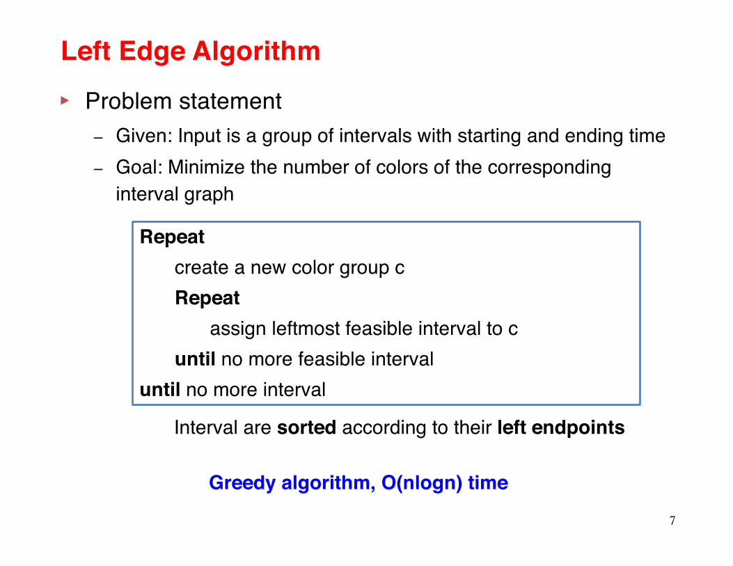
▸ Problem statement– Given: Input is a group of intervals with starting and ending time– Goal: Minimize the number of colors of the corresponding
interval graph
7
Left Edge Algorithm
Repeatcreate a new color group cRepeat
assign leftmost feasible interval to cuntil no more feasible interval
until no more interval
Interval are sorted according to their left endpoints
Greedy algorithm, O(nlogn) time

Left Edge Demonstration
Lifetime intervals with a given schedule
Assign colors (or tracks) using left edge algorithm
0 1 2 3 4 5 6 7
16
47
8
2
35
8
6
7 4
2
1
3
5
Colored conflict graph8
0 1 2 3 4 5 6 7 8
8
1 2 3
6 7 5
4
8

9
Binding Impact on Multiplexer Network
Functional Unit Operations
Mul1 op1, op3AddSub1 op2, op4AddSub2 op5, op6
clock cycle
×
×
+
+ +−
2 3 41
a
b
cdefg
op1op2
op3
op4
op5
op6
Functional Unit Operations
Mul1 op1, op3AddSub1 op2, op4, op6AddSub2 op5
Binding 1 Binding 2
+
×
+
a
Mul1
AddSub1
AddSub2
d b e
c
f g+
×
a
Mul1
AddSub1
d b e
c
+AddSub2
f g

Binding Algorithms to Optimize MUX Network▸ The connectivity binding problem is NP-Hard
– Exact ILP formulations available but not scalable
▸ Graph-based heuristic algorithms– Clique partitioning [Tseng CAD’86] [Paulin DAC’86]– Bipartite [Huang DAC’90]– Min-cost network-flow [Chang DAC’95] [Chen ASPDAC’04] [Chen DAC’06]
▸ Meta-heuristics using simulated annealing, evolutionary algorithm, etc.– Pros: Consider multiple optimization parameters together for globally
better results – Cons: Run-time and scalability
10

▸ Resource sharing directly impacts the complexity of the resulting datapath– # of functional units and registers, multiplexer
networks, etc.
▸ Binding for resource usage minimization– Left edge algorithm: greedy but optimal for DFGs– NP-hard problem with the general form of CDFG – Polynomial-time algorithm exists for SSA-based
register binding, although more registers are required
▸ Connectivity binding is intractable11
Binding Summary

▸ Parallel processing– Emphasizes concurrency by replicating a hardware
structure several times• High performance is attained by having all structures execute
simultaneously on different parts of the problem to be solved
▸ Pipelining – Takes the approach of decomposing the function to
be performed into smaller stages and allocating separate hardware to each stage (Heterogeneous)• Data/instructions flow through the stage of a hardware pipeline at a
rate (often) independent of the length of the pipeline
Parallelization Techniques
[source: Peter Kogge, The Architecture of Pipelined Computers]12
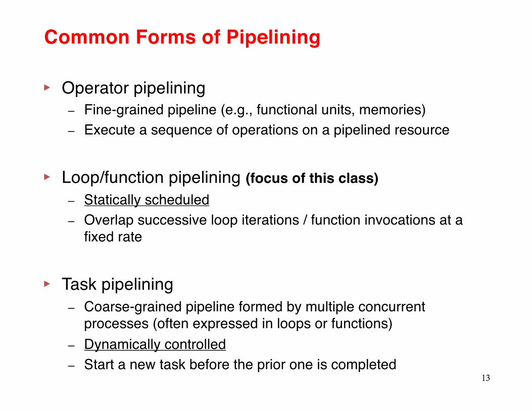
▸ Operator pipelining– Fine-grained pipeline (e.g., functional units, memories)– Execute a sequence of operations on a pipelined resource
▸ Loop/function pipelining (focus of this class)– Statically scheduled– Overlap successive loop iterations / function invocations at a
fixed rate
▸ Task pipelining– Coarse-grained pipeline formed by multiple concurrent
processes (often expressed in loops or functions)– Dynamically controlled– Start a new task before the prior one is completed
13
Common Forms of Pipelining

▸ Pipelined multi-cycle operations– v3 and v4 can share the same pipelined multiplier (3 stages,
latency = 2)
14
Operator Pipelining
+
×
×
-
+C0
C1
C2
C3
C4
C5
v1
v4
v2
v3
v5

Loop Pipelining
▸ Loop pipelining is one of the most important optimizations for high-level synthesis– Allows a new iteration to begin processing before the previous
iteration is complete– Key metric: Initiation Interval (II) in # cycles
15
for (i = 0; i < N; ++i)p[i] = x[i] * y[i];
II = 1
ldld
ld
× ××
××
×
stst
stld – Loadst – Store
ldld
×
st
x[i] y[i]
p[i]
Pipeline schedule
Pipelining

▸ Given a 100-iteration loop with the loop body taking 50 cycles to execute– If we pipeline the loop with II = 1, how many cycles do
we need to complete execution of the entire loop ?– What about II = 2 ?
16
Pipeline Performance
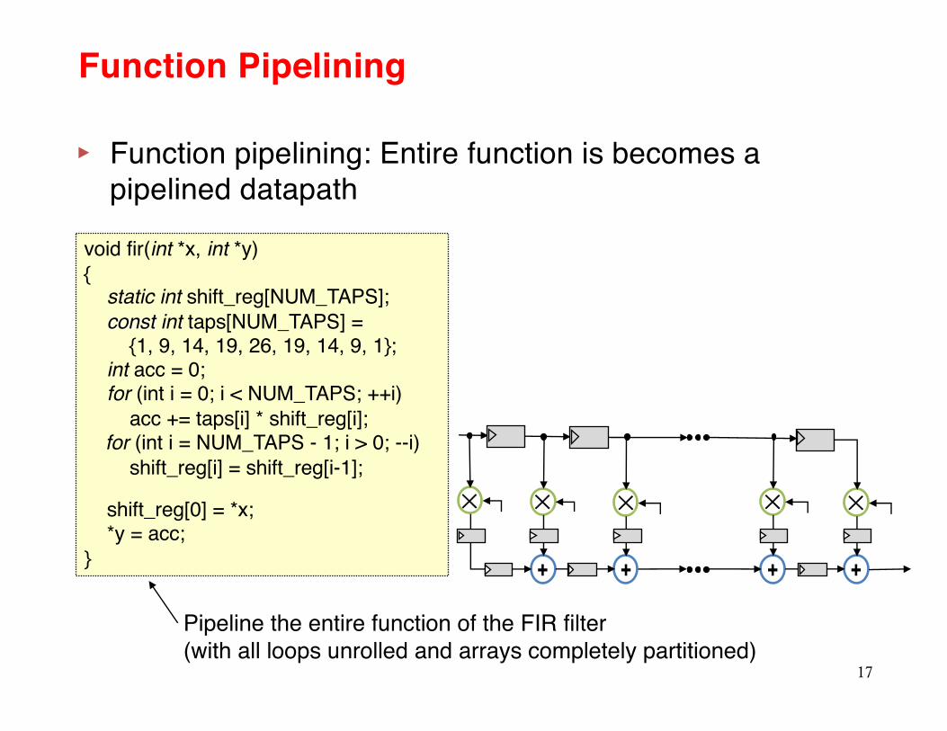
▸ Function pipelining: Entire function is becomes a pipelined datapath
17
Function Pipelining
void fir(int *x, int *y){static int shift_reg[NUM_TAPS];const int taps[NUM_TAPS] =
{1, 9, 14, 19, 26, 19, 14, 9, 1};int acc = 0;for (int i = 0; i < NUM_TAPS; ++i)
acc += taps[i] * shift_reg[i];for (int i = NUM_TAPS - 1; i > 0; --i)
shift_reg[i] = shift_reg[i-1];
shift_reg[0] = *x; *y = acc;
}
Pipeline the entire function of the FIR filter (with all loops unrolled and arrays completely partitioned)
×
+
×
+
×
+
×
+
×

Task Pipelining
GradientWeightingH
OuterProduct
GradientCalculation
VelocityCalculation
TensorCalculationV
gx
gy
gz
wy
wx
wz
oxy
oyy
oxx
oxzoyz
txy tyy txxtxztyz
DVI
frame_in frame_out
velXvelY
linebuffer linebuffer
linebuffer
GradientWeightingV
wy
wx
wz
TensorCalculationH
txy
tyy
txx
txztyz
18
A coarse-grained pipeline for the optical flow algorithm

▸ Resource limitations– Limited compute resources – Limited Memory resources (esp. memory port limitations)– Restricted I/O bandwidth– Low throughput of subcomponent…
▸ Recurrences – Also known as feedbacks, carried dependences– Fundamental limits of the throughput of a pipeline
19
Restrictions of Pipeline Throughput

20
Resource Limitation
▸ Memory is a common source of resource contention– e.g. memory port limitations
Only one memory read port à 1 load / cycle
for (i = 1; i < N; ++i) b[i] = a[i-1] + a[i];
Assuming ‘a’ and ‘b’ are held in two different memories
cycle 1 cycle 2 cycle 3 cycle 4i = 0 ld1 ld2 + sti = 1 ld1 ld2 +II = 1
ld2
+
ld1
st
a[i-1]
b[i]
a[i]
Port conflict

cycle 1 cycle 2 cycle 3 cycle 4i = 0 ld1
ld2+ st
i = 1 ld1ld2
+ st
▸ Recurrences restrict pipeline throughput– Computation of a component depends on a previous result
from the same component
21
Recurrence Restriction
for (i = 1; i < N; ++i) a[i] = a[i-1] + a[i];
II = 1
ld2
+
ld1
st
a[i-1]
a[i]
a[i]
ld – Loadst – Store
Assume chaining is not possible on memory reads (i.e., ld) and writes (i.e., st) due to cycle time constraint
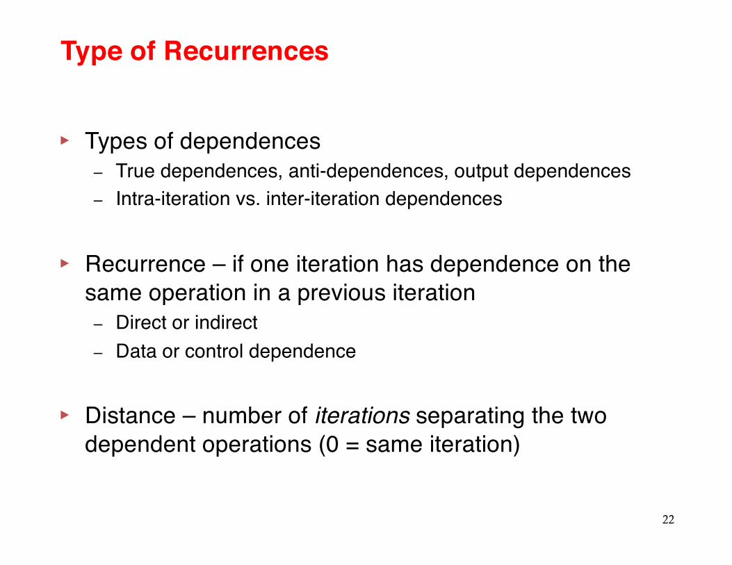
Type of Recurrences
▸ Types of dependences– True dependences, anti-dependences, output dependences– Intra-iteration vs. inter-iteration dependences
▸ Recurrence – if one iteration has dependence on the same operation in a previous iteration– Direct or indirect– Data or control dependence
▸ Distance – number of iterations separating the two dependent operations (0 = same iteration)
22

▸ True dependence – Aka flow or RAW (Read After Write) dependence – S1 àt S2
• Statement S1 precedes statement S2 in the program and computes a value that S2 uses
Example:
True Dependences
Inter-iteration true dependence on A[] (distance = 1)
23
for (i = 0; I < N; i++) A[i] &= A[i-1] - 1;

for (… i … ) {A[i-1] = b – a; B[i] = A[i] + 1
}
Anti-Dependences
▸ Anti-dependence– Aka WAR (Write After Read) dependence – S1 àa S2
• S1 precedes S2 and may read from a memory location that is later updated by S2
– Renaming (e.g., SSA) can resolve many of the WAR dependences
Example:
24
Inter-iteration anti-dependence on A[] (distance = 1)

Output Dependences
▸ Output dependence– Aka WAW (Write After Write) dependence – S1 precedes S2 and may write to a memory location that is later
(over)written by S2 – Renaming (e.g., SSA) can resolve many of the WAW dependences
Example:
25
for (… i++) {B[i] = A[i-1] + 1A[i] = B[i+1] + bB[i+2] = b – a
} Inter-iteration output dependence on B[](distance = 2)

▸ Data dependences of a loop often represented by a dependence graph– Forward edges: Intra-iteration (loop-
independent) dependences– Back edges: Inter-iteration (loop-carried)
dependences– Edges are annotated with distance values:
number of iterations separating the two dependent operations involved
▸ Recurrence manifests itself as a circuitin the dependence graph
26
Dependence Graph
v1
v2
v4
v3
[1]
[0] [2][0]
[0]
Edges annotated with distance values
[0]

▸ Next lecture: More pipelining (modulo scheduling)
27
Before Next Class


![Pipelining & Parallel Processing - ics.kaist.ac.krics.kaist.ac.kr/ee878_2018f/[EE878]3 Pipelining and Parallel Processing.pdf · Pipelining processing By using pipelining latches](https://static.fdocuments.in/doc/165x107/5d40e26d88c99391748d47fb/pipelining-parallel-processing-icskaistackricskaistackree8782018fee8783.jpg)