
MOODY’S MORTGAGE METRICS PRIME · Moody’s Mortgage Metrics Prime model, ... interest cashflows...
61
MOODY’S MORTGAGE METRICS PRIME: A QUASI-STRUCTURAL MODEL OF PRIME MORTGAGE PORTFOLIO LOSSES TECHNICAL DOCUMENT 1 July 2, 2010 Roger M. Stein Ashish Das Yufeng Ding Shirish Chinchalkar ABSTRACT This document outlines the underlying research, model characteristics, data, and validation results for Moody’s Mortgage Metrics Prime, which is an analytic tool for assessing the credit risk of a portfolio of prime residential mortgages. Moody’s Mortgage Metrics comprises loan-level econometric models for default, prepayment, and severity. These models are integrated through common dependence on local macro-economic factors, which are simulated at national, state, and Metropolitan Statistical Area (MSA) levels. This integration produces correlation in behaviors of loans across the portfolio. The simulation incorporates a multi-step Monte Carlo approach which enables the model to be combined with an external cashflow waterfall tool and used for simulation of RMBS transactions. Furthermore, we model both primary (loan-level) and secondary (pool-level) mortgage insurance. The resulting tool can be used to aid in analyzing the credit risk in RMBS as well as mortgage portfolios of whole loans. © 2010 Moody’s Research Labs. All rights reserved. Moody’s Mortgage Metrics® 1 Many past and present members of the current research group made significant contributions to the building and implementation of the Moody’ s Mortgage Metrics Prime models. Xufeng (Norah) Qian and Weijian Liang helped build the prepayment models. Weijian Liang also helped estimating the severity model. Jordan Mann helped model MI. Pouyan Mashayekh helped model the macro economic factors. Samuel Ring, together with Grigory Enenberg and Tamara Lubomirsky helped in the validation exercises. Xufeng (Norah) Qian, Jipil Ha, and Aziz Lookman helped in drafting some sections of this paper. We are grateful for their contribution and for the comments of Navneet Agarwal, Jordan Mann, Albert Metz, Rajesh Shekhar, and numerous members of the Moody’s Investors Service RMBS Surveillance team.
Transcript of MOODY’S MORTGAGE METRICS PRIME · Moody’s Mortgage Metrics Prime model, ... interest cashflows...

MOODY’S MORTGAGE METRICS PRIME:
A QUASI-STRUCTURAL MODEL OF PRIME MORTGAGE PORTFOLIO
LOSSES
TECHNICAL DOCUMENT1
July 2, 2010
Roger M. Stein
Ashish Das
Yufeng Ding
Shirish Chinchalkar
ABSTRACT
This document outlines the underlying research, model characteristics, data, and validation
results for Moody’s Mortgage Metrics Prime, which is an analytic tool for assessing the
credit risk of a portfolio of prime residential mortgages. Moody’s Mortgage Metrics
comprises loan-level econometric models for default, prepayment, and severity. These
models are integrated through common dependence on local macro-economic factors,
which are simulated at national, state, and Metropolitan Statistical Area (MSA) levels. This
integration produces correlation in behaviors of loans across the portfolio. The simulation
incorporates a multi-step Monte Carlo approach which enables the model to be combined
with an external cashflow waterfall tool and used for simulation of RMBS transactions.
Furthermore, we model both primary (loan-level) and secondary (pool-level) mortgage
insurance. The resulting tool can be used to aid in analyzing the credit risk in RMBS as
well as mortgage portfolios of whole loans.
© 2010 Moody’s Research Labs. All rights reserved. Moody’s Mortgage Metrics®
1 Many past and present members of the current research group made significant contributions to the building and implementation of the Moody’s Mortgage Metrics Prime models. Xufeng (Norah) Qian and Weijian Liang helped build the prepayment models. Weijian Liang also helped
estimating the severity model. Jordan Mann helped model MI. Pouyan Mashayekh helped model the macro economic factors. Samuel Ring, together with Grigory Enenberg and Tamara Lubomirsky helped in the validation exercises. Xufeng (Norah) Qian, Jipil Ha, and Aziz Lookman
helped in drafting some sections of this paper. We are grateful for their contribution and for the comments of Navneet Agarwal, Jordan Mann,
Albert Metz, Rajesh Shekhar, and numerous members of the Moody’s Investors Service RMBS Surveillance team.

Moody’s Mortgage Metrics Prime Technical Document (2010) 2 of 61
TABLE OF CONTENTS
1 INTRODUCTION ............................................................................................................................................... 3
1.1 Key findings .................................................................................................................................................. 5
2 MODEL COMPONENTS ................................................................................................................................... 6
2.1 A quasi-structural model of portfolio losses .................................................................................................. 6 2.2 Summary of the framework ........................................................................................................................... 7 2.3 Use in evaluating cashflow RMBS transactions .......................................................................................... 10 2.4 The meaning of “expected loss” .................................................................................................................. 11 2.5 The general specification for default and prepayment models .................................................................... 11 2.6 The variable selection process ..................................................................................................................... 15 2.7 Summary of key factors in the models ........................................................................................................ 21 2.8 Model variables: The default model factors ................................................................................................ 22 2.9 Model variables: The prepayment model factors ......................................................................................... 24 2.10 The severity model: LGD for mortgage loans ............................................................................................. 28 2.11 Treatment of mortgage insurance (MI) ........................................................................................................ 31 2.12 Econometric models of the state of the economy ........................................................................................ 33
2.12.1 Interest rates (CMT 10 year & LIBOR Six-months) ........................................................................... 34 2.12.2 House price change and Unemployment rate ...................................................................................... 35 2.12.3 Freddie Mac (FHLMC) mortgage rate ................................................................................................. 37
2.13 Incorporating delinquencies and realized pool performance ....................................................................... 38 2.14 Enhancements based on expert judgment .................................................................................................... 40 2.15 Frailty........................................................................................................................................................... 41 2.16 Estimating Loss Distribution using Monte Carlo simulation ....................................................................... 42
2.16.1 Estimation of the loss distribution ....................................................................................................... 42 2.16.2 The use of lagged values during simulation ......................................................................................... 43
2.17 Analyzing the Loss Distribution .................................................................................................................. 44 2.17.1 Expected loss for a tranche .................................................................................................................. 45
3 DATA .................................................................................................................................................................. 47
3.1 Data mapping and cleaning .......................................................................................................................... 48 3.2 Sample descriptive statistics ........................................................................................................................ 49
4 MODEL VALIDATION ................................................................................................................................... 50
4.1 Sensitivity Tests ........................................................................................................................................... 51 4.2 Predicting defaults for known macroeconomic paths .................................................................................. 54 4.3 Comparing model predictions to analyst estimates ...................................................................................... 57
5 CONCLUSIONS ................................................................................................................................................ 58
6 REFERENCES .................................................................................................................................................. 59

Moody’s Mortgage Metrics Prime Technical Document (2010) 3 of 61
1 INTRODUCTION
Moody’s Mortgage Metrics Prime is an analytic tool to help assess the credit risk of RMBS as
wells as mortgage portfolios of whole loans. This document describes the development of the
Moody’s Mortgage Metrics Prime model, including the data used, the modeling techniques and
the key challenges in building this model as well as our efforts to address them. It also
documents the model architecture, how the model may be used in practice and its capabilities.
Moody’s Mortgage Metrics analyses mortgage portfolios in four steps. First, it generates
trajectories of economic scenarios at a quarterly frequency over ten year horizon. Next, for each
loan in the portfolio, the models calculate quarterly default and prepayment probabilities over a
ten-year period as a function of loan-specific and economy-wide factors. Given these
probabilities, the software then simulates default events, prepayment events, and loss given
default and aggregates the simulated losses across all loans in the portfolio for each trajectory.
Finally, these simulated losses are themselves aggregated across all trajectories to produce an
estimate of the distribution of pool-level losses. Historical economic data used for the
simulations are updated quarterly.
Moody’s Mortgage Metrics’ capabilities include:
1. Estimating the impact of economic stresses on loan performance. The loan-
level models explicitly capture the relationships among loan characteristics and
economic states of the world. These relationships can be reported in detail for any
simulation. As a result, model output facilitates understanding the impact of key
economic factors on a pool-specific basis. This is particularly useful since the
same economic factor may have different effects in different pools due to the
interplay of key factors in determining loan behavior.
2. Capturing layered risks. In evaluating a mortgage pool, it is important to
examine layers of risk (the combined effects of various factors, including the
FICO scores, loan age, CLTV). The integrated structure of the models allows a
user to examine the impact of simultaneously changing multiple characteristics, as
well as the impact of factors that have competing effects (e.g., on prepayment vs.
default) on loan losses.

Moody’s Mortgage Metrics Prime Technical Document (2010) 4 of 61
3. Implementing multi-step analysis. Because the simulation engine produces
economic scenarios for each period between origination and the simulation
horizon, a richer representation of mortgage risk is possible. For example, since
the prepayment, default and recovery behavior of mortgages is time dependent,
dips in home prices that occur in an early period, may have very different
implications than those that occur in later periods. A multi-step Monte Carlo
simulation can differentiate between such cases.
4. Modeling mortgage insurance (MI). We model the impact of primary (loan-
level) and secondary (pool-level) mortgage insurance on loss given default (LGD).
Since LGD is stochastic and since mortgage policies may be written differently
for different loans, the impact of MI is more richly captured than might be the
case with a constant haircut to LGD. Furthermore, the impact of MI on a
particular loan may also vary significantly across economic states. By modeling
MI as a feature of individual loan we more naturally reflect both the contingent
(on the economic state) behavior of the insurance policy and the variability
associated with each policy. This also captures the interaction between primary
and secondary MI for a given pool.
5. Providing a framework that may be integrated with other tools for RMBS
analysis. The model simulates the losses and payments for each loan in each
period of the simulation. Thus, the model can be integrated with cashflow
waterfall tools to provide a detailed assessment of loss timing, interest cashflows
and amortization payments. This is important for synchronizing loss behaviors
across assets and liabilities for RMBS transactions.
6. Presenting increased transparency of mortgage portfolio risk. The model
offers lenders, investors, risk managers, securities issuers and intermediaries
detailed insight into the specific economic factors and loan characteristics that
affect a pool’s risk profile. Users can calculate Value-at-Risk and perform risk
factor attribution. Users can also evaluate pool losses based on custom scenarios
so that they may conduct stress testing under scenarios of particular interest to
them.2
2 This feature is currently not part of the standard software offering, but can be done as a service.

Moody’s Mortgage Metrics Prime Technical Document (2010) 5 of 61
1.1 Key findings
Modeling default, prepayment, and severity processes at the loan-level (as opposed to
the pool-level) significantly improves accuracy in estimating losses, particularly for
pools with heterogeneous mortgage assets.
Modeling each loan behavior separately (i.e., default, severity and prepayment as well
as mortgage insurance terms) provides far greater flexibility in calibration than using a
single joint model. Although prepayment, default and severity are distinct processes, the
modular approach uses common factor dependencies that permit it to capture the natural
interrelationships among the processes.
Prepayment can have a dominant effect in determining the distribution of losses during
periods of home price appreciation and/or falling interest rates. While default and
severity are key processes in loan behavior, without adequately understanding
prepayment, losses are difficult to understand over long cycles.
In addition to loan-specific characteristics, the state of the local and national economy
significantly impacts the performance of pools, with the key macro variables being
levels of home prices, unemployment rate, and interest rates.
Default, prepayment, and severity appear to be correlated through their joint dependence
on common economic factors.
The multi-step approach to simulation offers advantages when assets have time
dependent behavior, as in the case with mortgages.
The Moody’s Mortgage Metrics Prime model is intended to be help users better
understand the risks of prime mortgage pools. It should be used as a supplement to rather
than a substitute for a rigorous analytic process.
The remainder of this paper proceeds as follows: Section 2 provides an overview of the various
econometric models that make up Moody’s Mortgage Metrics Prime. Section 3 describes the
data and discusses the data collection and quality process. Section 4 discusses some of the
validation processes used to test the models. Finally, Section 5 summarizes our results and
provides some concluding thoughts on the models.

Moody’s Mortgage Metrics Prime Technical Document (2010) 6 of 61
2 MODEL COMPONENTS
In this section, we describe the loan-level models for default, prepayment, and severity and the
simulation framework used to integrate the output of these models in order to estimate the loss
distribution for a mortgage pool. Section 2.1 discusses the model framework in non-technical
terms, and Sections 2.2 through 2.6 provide some general background on the modeling
techniques. Sections 2.8 through 2.12 provide technical details on each of the component models.
Sections 2.13 through 2.15 discuss additional modeling considerations.
2.1 A quasi-structural model of portfolio losses
To adequately estimate the loss behavior of prime mortgage pools, it is useful to model at the
loan level the processes that affect losses: default, prepayment, and severity. Many market
participants intuitively contemplate default and severity when characterizing loan pool behavior.
However, the prepayment behavior of borrowers also has a first-order impact on pool losses.
This is because a loan with a lower prepayment probability is likely to remain outstanding for a
longer period of time making it more likely to default. That is, for a given level of default
intensity, higher prepayment rates result in lower losses over the lifetime of the pool. Hence, we
model prepayment as a risk that competes with default risk.
It is natural to think of these processes as being inter-related. For example, a drop in home prices
(home price depreciation) can
increase severity (lower recovery expected when the home value declines leading to
lower liquidation prices in the foreclosure process);
decrease prepayment likelihood (it is less likely that the borrower has enough remaining
home equity available for the borrower to refinance and the incentive to do so is reduced);
and
increase default likelihood (home owners without equity in their homes are less likely to
see the economic value in continuing to maintain their mortgages).
We incorporate these inter-relationships in our framework by using a common set of macro-
economic factors (in addition to loan-specific characteristics) to model the default, prepayment,
and severity processes. We use macroeconomic factors at the national, state or Metropolitan

Moody’s Mortgage Metrics Prime Technical Document (2010) 7 of 61
Statistical Area (MSA) level. This greater transparency of the drivers of portfolio losses and a
straightforward mechanism for conducting macro-economic scenario analysis provides more
flexibility in modeling new types of collateral. It also offers an implicit way of modeling
correlation in loan performance across the loans in a portfolio.
We combine information about the state of the economy with loan-specific information to assess
the risk of an individual mortgage loan since it is the interaction of macro and loan-level factors
that determines the performance of the loan. For example, lower interest rates (a macro factor)
tend to lead to higher probabilities of prepayment. However, even when interest rates are low,
loans for which the mortgage coupon (a loan-level factor) is higher relative to the prevailing
market rate are even more likely to prepay. Therefore, the level of interest rates alone is not a
sufficient predictor of prepayment. A model needs to consider the level of interest rates relative
to the borrower’s current coupon rate. Accordingly, we construct our measure of the mortgage
premium for use in the models by comparing interest rates to coupon rates on a loan-by-loan
basis rather than simply constructing a common measure based on interest rates alone.
The default, prepayment, and severity models are combined using a simulation engine that
generates scenarios of economic states of the world for the three broad sets of macro-economic
factors.
The three categories of macro-economic factors used:
National, state-, and MSA- level home price changes;
National, state-, and MSA- level unemployment rates ; and
Interest rates, including the term structure of Treasury rates, the 6 month LIBOR rate and
the Survey of Freddie Mac’s Prime Mortgage 30-Year Fixed Rate.
2.2 Summary of the framework
Moody’s Mortgage Metrics Prime is composed of a series of loan-level econometric models that
are related through common dependence on macroeconomic as well as loan specific factors. The
macro factors used in the loan-level models are simulated at the national-level, state-level and
MSA-level using econometric models developed for these factors.3 Using these loan-level
models, Moody’s Mortgage Metrics Prime estimates the loss for a loan given a realization of the
economic factors. Losses for this realization of economic factors are then aggregated across 3 Moody’s Mortgage Metrics simulates MSA-level estimates for the 60 MSAs that Moody’s has determined are most common in RMBS transactions. For loans that do not fall into those MSAs, Moody’s Mortgage Metrics uses state-level information.

Moody’s Mortgage Metrics Prime Technical Document (2010) 8 of 61
loans in the pool to produce an estimate of the pool loss under that specific economic trajectory.
Pool losses are aggregated across the simulations to estimate the expected lifetime loss and the
distribution of losses under all trajectories for the mortgage portfolio. In the current
implementation, the simulation is conducted over a 10-year horizon at a quarterly frequency
using 10,000 equally-weighted simulated economic paths to produce default rates, prepayment
rates and severity for each loan in the portfolio under each state of the world simulated. Figure 1,
below, summarizes this process schematically. In addition to computing losses across simulated
economic paths, the tool can be used to estimate losses under one or more specific pre-defined
forecast scenarios as well.
Figure 1: Interaction of econometric models
The process flow shown in Figure 1 is repeated each quarter over each simulated economic path as
shown in Figure 2. The computation progresses over a single path, one period at a time, for each
loan in the portfolio. Results of the loan-level loss estimates are aggregated across all loans in the
portfolio for that path to provide a loss value for the portfolio in that economic state. This
computation is then repeated until the end of each path is reached (pseudo-code for the algorithm
is given in Box 1). The distribution of these portfolio loss estimates forms an estimate of the loss
distribution.
Output
FACTORS
Loan Level Pool Data (User data)
Supplemental user data (Pool performance, etc.)
Economic Data (Simulated or realized)
Pool Leve
l E(L
)
Default
Severity
Prepayment
Loa
n Leve
l E(L
)
MODELS

Moody’s Mortgage Metrics Prime Technical Document (2010) 9 of 61
Figure 2: Calculation of Losses Based on Simulation of Different Trajectories of Economic Factors
The starting point for the economic simulations is the most recently available economic data,
which is currently updated each quarter. The scenarios for economic factors are generated over
the subsequent (future) 40 quarters.
Briefly, the macro-economic factors are modeled as follows:
the base interest rate (U.S. Treasury) is modeled using a two factor Cox-Ingersoll-Ross
(CIR) term-structure model;
the home price and unemployment projections are modeled using auto-regressive models,
where projections for a quarter are based on the previous two quarters of unemployment and
home prices data, respectively, as well as the 10-year Treasury;

Moody’s Mortgage Metrics Prime Technical Document (2010) 10 of 61
Box 1: The outline of the multi-step Monte Carlo simulation
1. For each economic scenario
a. Generate one realization of macro-economic variables over the next 40 quarters
i. For each loan
1. For each quarter
I. If the loan has not defaulted, prepaid, or fully amortized
i. Calculate the loan level probability of default, d
ii. Calculate the loan level probability of prepayment, p
iii. Generate a uniform random number, u, in the range (0,1)
iv. Determine whether the loan defaults in this quarter (u<=d)
1. If default
a. mark loan as defaulted
b. determine loan-level severity
c. record a loss
v. Determine whether the loan prepays this quarter (d<u<=d+p)
1. If prepay, mark loan as prepaid
II. End If
2. End of quarter
ii. End for each loan
b. Sum losses for all loans to arrive at pool loss for this economic scenario
2. End for each economic scenario
3. Calculate loss distribution (every point in the distribution represents the pool loss under a single economic
scenario)
2.3 Use in evaluating cashflow RMBS transactions
Since the simulator performs multi-step Monte-Carlo (i.e., it computes losses at a quarterly
frequency for simulated paths), it can produce quarterly cash flows for each loan under each
simulated path over the 10 year simulation horizon. Hence, it can also be used in conjunction
with an RMBS waterfall tool to produce detailed cash flow analyses for RMBS transactions.
Since the mortgage losses are driven by economic factors, the inter-relationships between the
assets and the liabilities of an RMBS transaction are naturally modeled. For example, high
interest rates depress prepayments and lead to higher default rates. The same high interest rates
can be used to calculate the interest payments due on the structured notes that occur
contemporaneously with the depressed prepayments and heightened default rates. Similarly, if
the timing of the increased default rates is such that it causes losses to occur later in the
transaction, the timing of the losses is naturally captured and waterfall triggers will be tripped in
the model as they actually would in such a setting. In contrast to the rather rich representation of
the behavior of the assets and liabilities modeled in this multi-step simulation, simpler
frameworks such as copula or single-step methods typically require the user to specify default
timing and severity curves in order to model the liability cashflows in structured transactions.

Moody’s Mortgage Metrics Prime Technical Document (2010) 11 of 61
2.4 The meaning of “expected loss”
The expected loss for a mortgage portfolio is the average loss that the pool experiences over the
horizon of analysis. The average is computed across the economic conditions simulated.
The expected loss is not necessarily the most likely loss outcome.
Confusion about what is meant by expected loss sometimes arises because the term expected is
sometimes used differently in statistics than in when it is used in the vernacular. In statistics it
means on average whereas in common conversation it is usually interpreted as meaning typical
or most likely.
As with many other credit-risky assets, in the case of mortgage portfolios, the expected loss is
often not the loss that will typically occur. In fact, the model predicts a wide variety of potential
losses, each of which will occur with some probability - the loss distribution. Averaging across
these possible loss outcomes produces mean loss, which is the estimate of the expected loss. The
most likely outcome is the mode of the distribution. For most credit-sensitive portfolios the modal
loss will be smaller than the mean loss.4
Credit portfolios with correlated assets tend to have skewed distributions. This means that in
most scenarios the observed loss will be less than the expected loss. However, there is a small
probability of experiencing losses that are much higher than the expected loss. Generally, we
might think of the lower losses happening in “normal” or “good” times and the larger losses
happen during times of stress. We anticipate this when we see a mortgage loss distribution, as
discussed in Section 2.16.
2.5 The general specification for default and prepayment models
We model two types of loan exit: default and prepayment. Both events are modeled using hazard
rate or survival models based on time-to-event data (the duration of time elapsed until the event,
default or prepayment, happens for the first time). Hazard rate models estimate the duration of a
loan’s survival rather than the probability of prepayment or default over a specified horizon
(although a transformation can convert the output from hazard rates to probabilities and vice-
versa). All loans are assumed to have the potential to prepay or default over a sufficiently long
4 A rule of thumb for most credit portfolio distributions is: mode < median < mean. For a perfectly symmetrical distribution all three measures will be equal.

Moody’s Mortgage Metrics Prime Technical Document (2010) 12 of 61
horizon. With time-to-event data, we use survival analysis to estimate the conditional probability
that a loan prepays or defaults over the next interval of time, where conditioning is done subject
to having survived up until that time.
Specifically, we use a semi-parametric Cox hazard model (Cox, 1972), in some cases augmented
with non-parametric techniques to better characterize the various behaviors of different types of
loans. Box 2 below gives a brief overview of the basic model. The Cox hazard models used in
this context make no assumptions about the shape of the baseline hazard rate function. This
flexibility is important given the unique impact that loan characteristics (e.g., reset periods) can
have on the underlying processes. This differs from simpler, but more constrained, parametric
survival models, such as Weibull, loglogistic, and exponential. The use of a non-parametric
method reduces the risk of model misspecification and provides much greater control over the
baseline hazard shape, thus capturing the observed peaks and troughs in the empirical
distributions more accurately. For example, it is known that different types of hybrid ARM loans
(5/25, 7/23 etc.) would have different prepayment peaks due to different reset timing, and thus
warrant different baselines. It is straightforward to capture different baseline patterns by loan
type using the semi-parametric Cox hazard model with stratification. This flexibility can be
difficult to achieve using a simple parametric model.
In our models, time-dependent variables are included (e.g., mortgage premium, home price
changes, etc.). Thus, the hazard ratios between loans are no longer constant over time due to the
changing factors. However, no interactions between time and other factors are used in the
default/prepayment hazard models so the effect of a unit change in the factors on the hazard ratio
is still constant over time.
Some of the loans in the data set are not observed completely from origination because they are
already seasoned when the data starts in 2001. Some others are not securitized until a few
months after their originations, and thus are seasoned when they appear in the data for the first
time. This phenomenon, called left truncation, has been well studied in the analysis of survival
data and a number of adjustments have been developed. In the case of the models we describe
here, we estimate the default/prepayment hazard rates in a time varying counting process manner
where left truncated loans only enter into the risk sets when they are observed.
In addition, right censoring is also present in mortgage pool data. Two types of right censoring
are addressed in our model:

Moody’s Mortgage Metrics Prime Technical Document (2010) 13 of 61
Type I: a loan stays in the data set during the entire observation period and, as of the last
observation, has neither defaulted nor prepaid.
Type II: a loan is terminated (due to default or prepayment) during the sample period but
due to the “other” (competing) risk. That is, if we are estimating a default model, the loan
leaves the data set because it prepaid. Since its exit is not due to default, this observation
must be treated as a censored observation with respect to default. Similarly, a defaulted loan
is treated as a censored observation in the estimation used in prepayment model.
An additional technical complication in the estimation involves the presence of possible "ties" in
the data. We observe data only at a monthly frequency. When incidence rates are high and/or the
number of observations is large, we often have multiple loans terminated at the same point in
time (that is, in the same month). These are termed "tied events" since there are multiple events
in a single “instant” of time. A key assumption of the standard Cox proportional hazard model is
that no two events occur at the same time. However, the standard Cox Proportional Hazard
model can be extended to accommodate ties through a number of approaches. We use Efron’s
method (Efron, 1977) to address the presence of ties.5
Once we have estimated the coefficients for the covariates, we estimate the baseline hazard rates.
We perform this estimation in a modified Bayesian framework, combining prior knowledge of
prepayment and default behaviors for various loan types with respect to loan age with data on the
empirical distributions of prepayment and default times. We estimate the baseline rates using
spline functions and non-parametric density estimation.6 Our results suggest that for modeling
prepayments spline functions fit the data better and capture the known turning points more
efficiently. Examples of such turning points include a peak around month 12, which reflects
increased prepayments due to credit curing, and a peak around the reset date for ARMs (e.g., a
peak is observed around month 60 for 5/25 ARM loans). (See Section 2.9 for additional
prepayment patterns due to different reset times and prepayment penalty terms.). Splines also
represent the functional form more compactly making them attractive computationally.
5 In the survival analysis literature a number of methods for addressing ties has been suggested. Three methods are commonly used by practitioners: Kalbfleisch and Prentice’s exact method (Kalbfleisch and Prentice, 1980), Breslow’s approximation (Breslow, 1974), and Efron’s
approximation (Efron, 1977). When there are many such tied events, Kalbfleisch and Prentice’s (1980) exact method is computationally
inefficient. On the other hand, Breslow’s (1974) approximation is most efficient computationally but its estimations are relatively more biased than the other two. We use Efron’s (1977) method since its results are closer to the exact results than Breslow’s but involve a trivial increase in
the computation time.
6 Interested readers can find references on these topics from many sources, e.g. Hastie and Tibshirani (2001) and Siminoff (1996).

Moody’s Mortgage Metrics Prime Technical Document (2010) 14 of 61
Box 2 Cox Proportional Hazard Model
Survival specifications directly model the duration of survival (rather the presence or absence of a
default or prepayment event at a given horizon). The fundamental quantity of a survival model is the
hazard function, also known as conditional failure rate. tthi )( is approximately the probability at time
t that the event will occur for loan i in the next small time interval, t . For continuous survival data,
the hazard rate is the instantaneous risk that an event will occur to subject i at time t, given that the
subject survives to time t:
t
tTttTtPth ii
ti
)|(lim)(
0
hi(t) is restricted to be nonnegative.
Survival models can be viewed as ordinary regression models in which the dependent variable is taken
as the time until the occurrence of an event. However, the computation of the likelihood function is
complicated by the censoring of the observations over time. Censoring is a common feature of survival
data. Complete observation of the exit time T for each subject is not always possible. Unless a loan
matures during the observation period, the loan’s exit time is observed only if a loan is terminated:
either prepaid or defaulted.
If a loan has not yet prepaid or defaulted by the end of the observation period, the time to the event is
after the time it could be observed as having prepaid or defaulted. For this loan, the time-to-event is
treated as a censored observation. In addition to censoring at the end of the sampling period,
observations can be censored at any time point during the sample period due to competing risks.
The Cox Proportional Hazards model is a popular survival model. Given the covariate vector xi, the
conditional hazard function for loan i is defined as
( )
0( ) ( ) if
ih t h t eβ' x
where f(x) are the transformed factors, and h0(t) denotes the baseline hazard function. This is the hazard
when all transformed covariates are zero. We use a single f to denote the transformations for notational
simplicity. However they may be different for each factor.
Under this formulation, across all loans there is a baseline hazard rate that varies with the age of the
loan (time since origination). A particular loan’s hazard rate is based on the baseline but is increased or
decreased due to the attributes of the loan, borrower and property and the state of the economy.
In the plain vanilla Cox model described above, the covariates are static over time, so the ratio of the
estimated hazards over time will be constant, thus it is referred as the “proportional” hazard model. It
has been shown (Cox (1972,1975)) that, by eliminating the infinite dimensional nuisance parameter
from the full likelihood, we can estimate β, the vector coefficients, based on a partial likelihood
approach without explicit knowledge of the baseline function, h0(t).
Time-dependent covariates are used in our implementation (e.g., mortgage premium, home price
change, etc.). This would result in a non-proportional hazard relationship between two loans over time
due to the changing factors. However, no interactions between time and other factors are used in the
default/prepayment hazard models. As a result, the effect of a unit change in the factors on the hazard
ratio is still constant over time.

Moody’s Mortgage Metrics Prime Technical Document (2010) 15 of 61
2.6 The variable selection process
A long list of variables potentially explains different aspects of loan performance. We base our
selection on factors identified as important by academic researchers, industry participants,
RMBS analysts and modelers, and, importantly, the quantitative properties of the factors (e.g.,
robustness and predictive power).
In general, we use economic reasoning to guide the factor selection rather than relying solely on
statistical correlation. For example, consider again the impact of the prevailing interest rate on
prepayment, which we discussed in Section 2.1. As it turns out, the absolute level of interest
rates is statistically related to prepayment for the time period of our data. However, we find the
simple “regression” relationship between levels of interest rates and prepayment less informative
than when the relationship is understood through its effect on the economic drivers of
prepayment. In this case, interest rates affect prepayments through the spread between a
borrower’s current mortgage rate and the prevailing rate. When this spread decreases – the
borrower becomes relatively better off since the opportunity cost of not refinancing becomes
smaller – there is lower incentive to prepay; when the spread between the current mortgage rate
and the prevailing interest rate increases there is greater incentive to prepay. Therefore, the same
rate level may affect different borrowers’ propensity to prepay differently. This observation leads
us to construct loan-specific measures for the impact of interest rate on prepayments rather than
simply using the interest rate itself as the simple “regression” relationship would have suggested.
As another example, consider the macro-variable, home price changes. In conjunction with
information about the loan and property, it can be used to infer the borrower’s updated LTV,
which has a theoretically sound relationship to both default and severity. The use of transformed
versions of the raw variables results in models that are more stable and have greater predictive
power.
Even when a macro-economic factor enters the model directly, rather than through other factors,
economic reasoning provides guidance in deciding how this factor should be used as an
explanatory variable (i.e., level, difference, lag, etc). For example, such reasoning motivates us
to use the cumulative change in home prices since the loan was originated rather than simply the
level of home prices.
Of course, in addition to having attractive theoretical, statistical and predictive properties, factors
must also be practically implementable from a business perspective.
Moody’s Mortgage Metrics Prime Technical Document (2010) 16 of 61
In summary, our criteria for selection of explanatory factors are:
Common sense/Economic theory. There should be an economic rationale for using the factor
as described above.
Statistical robustness. A factor should:
o have coefficient whose direction (sign) and magnitude should be consistent with
economic reasoning; and
o have (relatively) low correlation with other factors in the model: a factor’s
inclusion should not introduce multicolinearity; For example, there are many
factors that can be used to measure borrower's stake in the property, such as
borrower equity and updated LTV. Since they are highly correlated, we only
include updated LTV in our models. As an aside, we have tried to select factors
that measure ratios (updated LTV in this example) to variables that measure
absolute levels (borrower's equity in this example).
Practical implementation. A factor should be:
o readily available: most institutions must be able to calculate the factor based on
data they maintain and are willing to provide. As an example, neither updated
FICO nor updated appraisal value is readily available to many market participants
since many lenders do not update them regularly.
o defined relatively unambiguously: most institutions must calculate the factor in a
similar manner or be able to do so based on some simple rules; Debt-to-income
ratio (DTI), for example, is not used in the model because it can be defined
differently across different lenders.
We select factors for each model based first on univariate analysis that examines the ability of
each factor to predict default or prepayment on its own. Then we use multivariate methods to
assess which these factors remain predictive in the presence of other factors in the model. Finally,
we perform out-of-sample tests that guide us against overfitting the model.
Univariate Analysis: Unlike multivariate regression analysis, univariate analysis does not
control for the effects of other variables. We examine the predictive power of individual
variables by determining the univariate relationship between each variable and the frequency of

Moody’s Mortgage Metrics Prime Technical Document (2010) 17 of 61
the specified event (default or prepayment). We use techniques similar to those described in
Falkenstein, Boral, and Carty (2000) and Dwyer and Stein (2004) for this analysis. We use a
number of non-parametric techniques (c.f., Hastie and Tibshirani (1990) and Siminoff (1996)) to
control for both remaining outliers and non-linearity in our data. Our approach follows the
following steps:
1. We rank all mortgage loans by a particular predictor variable. For time-varying
variables, we rank the monthly observations.
2. We then segment the loans into k bins, where k and the width (range of values for the
predictor variable) of each bin are determined by the distribution of the variable.
3. We then calculate the frequency of the event, default or prepayment, for each bin,
which results in a granular mapping from the predictor variable to the frequency of
the event. (This approach is commonly called bin smoothing.)
4. We then obtain a smoother estimate of the relationship by (non-parametrically)
smoothing across the bins. This approach smoothes the default/prepayment rates
across bins, while minimizing the prediction error for each bin. We use the mean
value of the predictor variable for each bin as the representative value for that bin.
5. For values that fall between the endpoints of a bin, we interpolate, using the density
estimate, to arrive at a value.
6. Finally, we examine both the nature of the relationship (slope, monotonicity, etc.) and
the univariate predictive power of this variable.7 We examine the latter using both the
density estimates of the relationship and by calculating power curves.
By reviewing the shape of the curve and the spacing of the bin boundaries, we seek to determine
whether the relation is in the expected direction or whether it is counterintuitive, suggesting data
issues may be present or that (for the segment of the population we are examining) the
theoretical relationship may not hold as strongly. We also get a sense of how significantly a
change in this variable level affects the probability of an event. If the slope of the curve is steep,
a small change in the levels of the factor will have a larger impact on the examined event than if
7 See Stein (2007) for a discussion of the relationship between density estimates and power.

Moody’s Mortgage Metrics Prime Technical Document (2010) 18 of 61
the slope is flat. Finally, we examine the extent to which the relationship is non-linear, which
would suggest using certain transformations. We now illustrate how we use the univariate
analysis.
As an example of the usefulness of the univariate mapping, Figure 3 provides the mappings of
some of the factors in the default models. Note how the transformation function is itself an
estimate of the default rates at each quantile. The lack of perfect agreement between the actual
points and the smoothed density estimate is not only due to sampling noise, but also due to the
fact that the factor is not a perfect predictor.
Figure 3: Univariate relationship of selected variables in the default model
The relationship for FICO (upper left) is monotone with a pronounced slope, suggesting high
predictive power for FICO. The downward slope is economically reasonable: we expect
borrowers with higher FICO score to have lower default rates. Similarly, the monotonic
relationships between default and mortgage premium and updated LTV are also intuitive. In

Moody’s Mortgage Metrics Prime Technical Document (2010) 19 of 61
contrast, the relationship between default and loan amount suggests strong association, but also
that loan amount by itself is probably not a good predictor. To address this, we also examine
interactions of two or more variables when they are economically sensible. For example, as
shown in Figure 4, loan amount is found to have much more intuitive relationship with default
rates when it is considered jointly with documentation.8
Figure 4: The impact of loan amount on default hazard depends on documentation
Multivariate analysis: Based on the univariate analysis, we rank variables from the most
predictive to the least predictive (while still consistent with economic intuition). We then
perform multivariate analysis. Because many variables are correlated to some degree, we also
evaluate whether the variables are too highly correlated to permit their joint inclusion in the
model. We do this using both inspection (e.g., whether the added variable changes the sign of the
coefficient of an existing variable in the model or whether the coefficient of the added variable
8 Together, loan amount and documentation indicate the degree to which a given loan agrees with prototypical notions of “Prime”.

Moody’s Mortgage Metrics Prime Technical Document (2010) 20 of 61
has the wrong sign) and through the use of formal statistical methods such as calculating
variance inflation factors (VIF).
We find that variables which have a strong monotonic relation in the univariate analysis are often
robust in multivariate analysis, provided we control for colinearity. The variables which exhibit
weak predictive power (an almost flat relation) in the univariate analysis will typically not be
statistically significant and may even have a coefficient with an unintuitive sign in the
multivariate estimation.
Parameter stability: In the course of multivariate estimation, we examine the stability of models
built using the selected factors. We subset the data into smaller time periods and estimate
coefficients for the multivariate model for each sub-period and examine the variation in value
and the statistical significance across the different sub- periods (we do this to establish parameter
stability, rather than to evaluate out-of-sample performance. Out-of-sample performance testing
is discussed in Section 4).

Moody’s Mortgage Metrics Prime Technical Document (2010) 21 of 61
2.7 Summary of key factors in the models
In Table 1 below, we summarize the key factors and their effects in the default, prepayment, and
severity models. The symbol “+” implies a positive relationship between the factor and the
corresponding model (default, prepayment, or severity) whereas a “–” implies an inverse
relationship.
Table 1: The key factors and their effects on default, prepayment, and severity models
Factor Default Prepayment
Severity FRM ARM
LTV – –
Updated LTV +
HPI Change + +
Forward LTV9 +
Junior LTV + – –
Mortgage premium at origination + + + +
Mortgage premium change + + +
Unemployment rate change +
Unemployment rate +
Payment shock of initial reset +
FICO – + +
Judicial state + +
Loan amount +/– +/– +/– –
Documentation10
Bad Doc >
Good Doc +/–
Good Doc >
Bad Doc
Loan type ARM > FRM
Prepayment penalty term – –
Burnout effect – –
Occupancy type
(relative to Owner
occupied)
Investment + – –
Second home + – –
Loan purpose
(relative to
purchase)
Rate-refi + – +
Cashout + – +
Debt
consolidation – –
Home
improvement – +
Property Type
(relative to single
family)11
Condo – + –
Co-op – – –
PUD – + +
Townhouse – + –
9 Please see Section 2.10 for the definition of forward LTV. 10 Documentation type interacts with the loan amount in FRM prepayment model and in the default model. 11 Only a few property types are mentioned here.

Moody’s Mortgage Metrics Prime Technical Document (2010) 22 of 61
2.8 Model variables: The default model factors
In our model, the definition of default is that
a loan’s reported status transitions to foreclosure;
a loan’s reported status transitions to real-estate-owned (REO);
the borrower declares bankruptcy; or
the borrower is more than 120 days past due on a mortgage payment and subsequently
enters one of the three states listed above.
The timing of default is determined as the earlier of foreclosure, REO, borrower’s bankruptcy or
120 days past due.
The default model is of the form of a semi-parametric Cox hazard model with time-dependent
variables (see Box 2), which include mortgage premium and updated LTV. Ideally one might
also wish to include time-dependent FICO in the default model, since the effect of original FICO
dampens over time. However, updated FICO scores are often not available since many lenders
do not refresh them regularly.
The most important factors for predicting defaults include FICO score, mortgage premium (both
the mortgage premium at origination and the change over time), updated LTV, junior LTV, loan
structure and loan size (A complete list of the factors in the default model is given in Section
2.7), and we discuss these briefly below.
FICO: FICO scores at loan origination (holding all other loan factors equal) are a strong
predictor of default levels. While the impact of FICO at origination declines over time, possibly
due to credit curing or FICO drift, it is a reasonable indicator of default risk even for seasoned
loans.
Mortgage Premium at origination: This variable is constructed as the spread between the
coupon rate and the market rate at the time of loan origination. The market rate is measured by
the survey of 30-year fixed rate mortgages given by Freddie Mac for prime borrowers. Loans
with a higher mortgage premium are likely to default for two reasons. First, loans with a higher

Moody’s Mortgage Metrics Prime Technical Document (2010) 23 of 61
mortgage premium are associated with higher coupon rates and therefore have higher debt
service burdens. Second, higher mortgage premiums suggest a greater level of credit risk at the
time of underwriting, perhaps due to borrower-specific factors that the lender may observe but
that may not be formally reported.
Change in Mortgage Premium: As mentioned above, mortgage premium at origination carries
additional risk information not captured by FICO, providing an additional measure of relative
credit worthiness of the borrower. If nothing else changes over time, a borrower is expected to be
able to avoid an increase in her mortgage premium (at least beyond transaction costs) through
opportunistic refinancing. Observing an increased mortgage premium thus suggests a troubled
borrower who is either unable to refinance or, for those same (unobserved) reasons, at greater
risk of default. It also suggests that the borrower’s financial burden may have increased, as
monthly payments are higher than at the time of origination.
Updated Loan-to-value: LTV is a measure of leverage for the loan. For newly-originated
purchase loans, LTV reflects the borrower’s down payment, which in turn tends to be a function
of the borrower’s long-term financial capacity and discipline and the borrower’s commitment to
the property. Updated LTV is calculated by updating the house price using the state- or MSA-
(when available) level housing price changes. This permits a more accurate time-varying
measure of borrower equity. Higher values of the updated LTV imply lower equity in the home
and, hence, reduced aversion to defaulting on the property.
The Loan Structure: Loan features can vary substantially across loans. These features,
including coupon resets, coupon levels, the presence or absence of a teaser rate, and amortization
terms, influence default behavior due to phenomena such as payment shock. (If, after a loan
resets, the interest rate rises significantly due to changes in market rates or the presence of a
teaser rate, this additional cost will impact default rates.)
Baseline Hazard Rate: The baseline describes the general trend of the default rates for
borrowers as a function of loan age. Default rates for prime mortgages tend to start low in the
first year after loan origination and then rise, peaking around the fifth year after origination. This
seasoning effect is reflected in the hump shape of the default baseline. All else equal, a loan
seasoned past this peak will have a lower life-time default risk than that of a newer loan. We use
different default baselines for ARM and fixed-rate mortgages (See Figure 5). The baselines of
the default models are estimated using non-parametric density estimation techniques. This
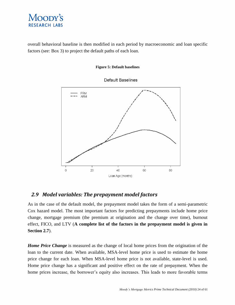
Moody’s Mortgage Metrics Prime Technical Document (2010) 24 of 61
overall behavioral baseline is then modified in each period by macroeconomic and loan specific
factors (see: Box 3) to project the default paths of each loan.
Figure 5: Default baselines
2.9 Model variables: The prepayment model factors
As in the case of the default model, the prepayment model takes the form of a semi-parametric
Cox hazard model. The most important factors for predicting prepayments include home price
change, mortgage premium (the premium at origination and the change over time), burnout
effect, FICO, and LTV (A complete list of the factors in the prepayment model is given in
Section 2.7).
Home Price Change is measured as the change of local home prices from the origination of the
loan to the current date. When available, MSA-level home price is used to estimate the home
price change for each loan. When MSA-level home price is not available, state-level is used.
Home price change has a significant and positive effect on the rate of prepayment. When the
home prices increase, the borrower’s equity also increases. This leads to more favorable terms

Moody’s Mortgage Metrics Prime Technical Document (2010) 25 of 61
for rate-refinancing or cash-out refinancing with lower LTV (due to increased home price).
Higher values of home equity also provide stronger economic incentives for the borrower to
prepay in order to benefit from the accumulated equity. The opposite is true in a falling home
price market as the borrower’s equity will diminish or even become negative. In a falling home
price market, therefore, both borrowers’ ability and incentive to prepay can be significantly
reduced.
Mortgage premium at origination is defined as the difference between the mortgage rate for a
loan and the prevailing average mortgage rate for prime mortgages (e.g., FHLMC rate). Loans
with a higher mortgage premium tend to have a higher prepayment rates. The reason for this is
twofold. First, a borrower with a higher premium on his loan has a greater incentive to refinance,
as his savings in financing costs (e.g., reduction in monthly payments) will be greater. Second, a
higher premium is associated with higher credit risk at origination. Over time, the
creditworthiness of borrowers that do not default typically improves because of credit curing,
which means the borrower may be able to refinance at a lower rate that better reflects the
improved creditworthiness.
Mortgage premium Change is defined as the change in the mortgage premium from the point of
origination of the loan. A positive change could be due to a decrease in the market rate or an
increase in the borrower’s coupon rate or both. In either case, the borrowers have greater
incentive to refinance.
Prepayment penalty clauses are provisions in the mortgage contract that require the borrower to
pay a penalty if she pays off the loan before a certain date. The penalty is paid only if the loan is
prepaid within a certain period of origination, referred to as the prepayment penalty period.
Loans with prepayment penalty clauses are significantly less likely to be prepaid prior to the
expiration of the prepayment penalty because the cost of this penalty may outweigh the long
term benefit of reduced monthly payments. Note that prepayment penalty clauses are not as
common for prime mortgages as for subprime or Alt-A mortgages.12
Burnout effect is meant to capture unobserved borrower-specific factors that may make it less
likely for a mortgage-holder to refinance, even in environments that favor refinancing. We model
this as a dummy variable which is set to value 1 when a borrower does not make use of, at least,
two refinancing opportunities over a period of eight quarters. We define a refinancing
12 In our data sample less than 4% of the loans have prepayment penalty clauses.

Moody’s Mortgage Metrics Prime Technical Document (2010) 26 of 61
opportunity as a quarter during which the loan is not in the prepayment penalty period and the
prevailing market rate is lower than the current coupon rate by more than 200 bps. Loans that
exhibit burnout are less likely to prepay in subsequent periods. If a borrower has decided not to
refinance when doing so would reduce the borrower’s financing costs, we assume that the
borrower is either insensitive to changes in mortgage rates or has other reasons to avoid
refinancing, and is therefore less likely to prepay the loan in the future.
FICO at origination is a significant predictor of prepayment, holding all other loan factors
constant. FICO measures the credit quality of an individual borrower. The higher the FICO score,
the higher the likelihood that the borrower could qualify for more attractive refinancing terms.
Furthermore, in periods of tighter lending, lower credit quality borrowers may have more
difficulty refinancing. The impact of FICO declines over time, possibly due to credit curing or
FICO drift.
LTV is a measure of leverage for the loan. LTV at origination is included in the model (together
with Junior LTV). For newly originated purchase loans, LTV reflects the borrower’s down
payment, which in turn tends to be a function of the borrower’s long-term financial capacity and
discipline and the borrower’s commitment to the property. The higher the LTV, the less equity a
borrower has in his house and the less flexibility he has in refinancing or selling the property.
Model Baseline Hazard Rates
Each model has an independent baseline. The baseline describes the general trend of the
prepayment rates for various loan categories, such as 5/25, fixed, and so on, purely as a function
of elapsed time. The loan specific factors and elements of the simulated economic paths are
overlaid on the behavioral baseline pursuant to the Cox hazard framework to determine the
modeled prepayment rate paths of each loan (see Box 2).
The observed prepayment behavior differs between fixed-rate and ARM loans. To accommodate
this, we estimated separate models for these two broad loan types. The ARM model was further
refined by stratifying various baselines that differ by loan type within the ARM type depending
on the structure (i.e. reset month). In general, there is a prepayment spike for both ARM and
fixed loans after one year (resulting from the credit curing of some borrowers). For ARMS there
is also generally second spike after a loan resets. Prepayment penalties can create additional
spikes.

Moody’s Mortgage Metrics Prime Technical Document (2010) 27 of 61
For example, in examining 5/25 loans with 24-month prepayment penalty terms, we observe a
prepayment peak around month 24 (prepayment penalty expires) followed by a pronounced
increase in prepayments in year 5, when the loan rate reset. If this heterogeneity is not addressed
in the model--for example, if one common baseline were used for the different loans--the peak
time would be biased and the bias would be proportional to the degree of heterogeneity in the
population.
Figure 6 gives some examples of the uncalibrated prepayment baselines for FRM and ARM
loans. These can be interpreted as being the general shapes of the prepayment hazard rates ( )
before calibration. These baselines are scaled upward or downward depending on loan and
borrower characteristics and the state of the modeled economy.
Figure 6: Baseline FRM and ARM Prepayment Rates
Since some of the loan-level factors used in our analysis depend on time-varying macro
economic factors (for instance, home price appreciation or interest rate factors), a different
adjustment is used for each quarter of an economic scenario. The effect of the adjustment
varying with time because of changing macroeconomic conditions is that the actual prepayment
curve for a specific loan typically looks like a “warped” version of the baseline.
( )P
ih t

Moody’s Mortgage Metrics Prime Technical Document (2010) 28 of 61
To give some sense of this, Figure 7, below shows the hazard rate h(t) of a single 5/25 loan in
different economic scenarios.
Figure 7 Prepayment hazard rate of a single loan in different economic paths
2.10 The severity model: LGD for mortgage loans
The severity or loss given default (LGD) is defined as the ratio of loss (as reported by originators
and servicers) to original balance of the mortgage loan. We compute the dollar loss by
multiplying severity by the original balance.

Moody’s Mortgage Metrics Prime Technical Document (2010) 29 of 61
While a body of literature exists describing modeling of loss given default for corporate
exposures (c.f., Gupton and Stein (2002, 2005)), Acharya, Sreedhar, and Srinivasan (2004) less
has been written on loss given default for retail exposures.13
However, there are similarities.
Clearly, both processes describe distributions of ratios. A common approach to modeling such a
process is to assume that the data generating process follows a Beta distribution, which is chosen
for several reasons. First, it can take a variety of shapes based on the choice of parameter values.
Second, the parameter values can be readily estimated using only the sample mean and sample
variance, which facilitates implementation of the model.
The distribution of severity in our sample, as shown in Figure 8, is consistent with the skewed
shape characteristic of the Beta distribution. A severity in excess of 100% seems improbably
high. In our data, more than 10% of the defaulted loans have such high severities. We examine
how loans could have greater than 100% severity. We find these severities typically arise in
cases where the loan amount is quite low and therefore the fixed costs associated with the
recovery process, including servicing advances, are higher than the expected recovery amount,
and thus severity exceeds 100%. This is consistent with the finding that smaller loans tend to
have larger percentage losses as reported by Qi and Yang (2008) and others. We discuss this
trend later in this article.
Figure 8: Distribution of loan severity
13 This has recently begun to change. See for example Qi and Yang (2008) and references therein.

Moody’s Mortgage Metrics Prime Technical Document (2010) 30 of 61
Given the observed beta-like distribution we use a methodology similar to that described in
Gupton and Stein (2002).14
First, the observed severities are transformed to follow an
approximate Normal distribution by first applying Beta distribution and then applying inverse
Normal transformation. Next, a linear regression is fit to the transformed values. Finally, an
inverse beta transformation is performed on the predicted values from the liner model to compute
the predicted severity.
The basic form of this model is:
1
'
ˆˆ( ), ,
ˆ ( )
i i
s
i i i i
s Beta z
z q X
where,
2 is distributed (0, )i iN , which makes the severity stochastic,
si is the severity of the ith
defaulted loan,
are the estimated parameters of the Beta distribution,
() and Beta()-1 and are the standard cumulative Normal and inverse Beta distribution
functions, respectively,
is a vector of parameter estimates,
is a set of loan specific and macro economic factors affecting severity for the ith
defaulted loan,
qi() is a set of transformation functions of the individual factors (the form of the
transformation may vary across factors.
14 Since the publication of Gupton and Stein (2002), more formal techniques have gained popularity in the statistics literature (c.f., Ferrari and Cribari-Neto, 2004), though the stability of these techniques appears to be lower than that of Gupton and Stein (2002) in some empirical settings.
ˆˆ ,
S
iX

Moody’s Mortgage Metrics Prime Technical Document (2010) 31 of 61
The key factors for predicting severity are:
Judicial regulation: This factor describes whether or not a loan is in a U.S. state that has
judicial regulations relating to loan foreclosure and default (these make it harder to
liquidate a property). This delay has a direct impact on the losses since the longer the
process to liquidation, the more cost is likely to be incurred.
Forward loan to value ratio: Loan to value ratio is updated using the simulated value of
the house as of the estimated liquidation date, which is assumed to be eighteen months
from the time of default if the loan is in a state with judicial regulations on loan
foreclosure, and twelve months after default otherwise.15
We found forward LTV to be
more predictive than the updated LTV at the time of default. This is because liquidation
takes time, and the house value can drop significantly between the time of default and the
time when the house is actually sold as part of the liquidation process.
Loan amount: We find that smaller loans tend to suffer a higher percentage loss,
presumably due to the fixed cost associated with the recovery process. This is consistent
with economic reasoning and some recent academic literature. Furthermore, our research
and discussions with mortgage servicers suggest that they also recognize this effect and
expend greater effort to recover losses on large loans than on smaller loans. In the limit, if
the property value is less than the fixed cost of recovery, there is little incentive for the
servicer to pursue the recovery.
Mortgage premium: A higher mortgage premium is associated with lower principal
payment (as a percentage of the fixed payments) and higher relative accruing loan
coupon payments; it may also indicate lower borrower quality (see Section 2.8 for details
on mortgage premium).
A complete list of the factors in the severity model is given in Section 2.7.
2.11 Treatment of mortgage insurance (MI)
In addition to considering “natural” determinants of severity, we model the impact of mortgage
insurance on loss given default. Mortgage insurance is a financial contract that pays the
15 The prediction for the value of the house in the future is done using our MSA-level model for house price appreciation. Section 2.12.2 provides more details on this.

Moody’s Mortgage Metrics Prime Technical Document (2010) 32 of 61
mortgage lender or an RMBS trust a contracted amount when an insured borrower defaults on a
mortgage loan. The purchaser of mortgage insurance typically makes periodic premium
payments to the insurer in exchange for this protection. The presence of MI reduces the severity
(and hence the losses) for the pool without affecting defaults and prepayments.
We model two broad types of mortgage insurance
1. primary or loan-level mortgage insurance which covers a portion of the loss incurred on
an individual loan; and
2. secondary or pool-level mortgage insurance which covers a portion of the losses incurred
by a pool of mortgages.
In order to explain our implementation, it is useful to first illustrate how MI works by describing
a simple mortgage insurance contract; the exact terms of specific contracts vary considerably.
Consider a primary MI policy with a coverage level of 30%. When a loan defaults, the insurer
pays out an amount equal to the gross loss times the coverage. The gross loss is calculated as the
sum of the unpaid principal balance at the time of default, any unpaid interest and some
additional costs. Even though the reimbursed amount is typically equal to the gross loss times the
coverage level, if the property is sold before the claim is paid, the reimbursed amount is capped
at the realized loss, which is the loss net of proceeds from the sale of the property.
For example, suppose a borrower defaults and the gross loss is $200,000 and the coverage level
is 30 percent. The insurer would pay $200,000 x 30% = $60,000. However, if the house were
sold for $150,000 before the claim is paid, the net loss would be $50,000 (200,000 – 150,000 =
50,000) and the insurer would only pay this smaller amount rather than the full $60,000.
Mortgage insurance policies may also be terminated for a variety reasons, including expiration of
the policy, passage of half of the amortization period of the loan (e.g., for 30-year fixed loan, if
15 years have elapsed), and the reduction of the outstanding balance below a certain limit.
Additionally, claims may be rescinded due to fraud or bad servicing. In our modeling, we
assume a constant rescission probability and randomly rescind claims during the simulation with
that probability.

Moody’s Mortgage Metrics Prime Technical Document (2010) 33 of 61
In contrast to primary MI which applies to a specific loan, as described above, secondary MI
applies to the entire pool balance and covers losses incurred after primary MI, if any, has been
applied. There is usually a pool-level deductible. In addition, there are limits to the losses
covered for any one loan and to the total loss covered for the pool. As with primary MI, claims
may be rescinded due to fraud or bad servicing and they may be rescinded simply because the
primary MI claim was rescinded.
Secondary MI adds considerable complexity to the modeling of severity. When calculating the
reimbursement to be paid by the secondary MI policy for a given defaulted loan, it is necessary
to know whether the policy’s pool-level deductible has been met yet, and if so, whether the pool-
level loss limit has been met yet. Thus we can only calculate the reimbursement (and hence the
severity) for the given loan if we know the loss and reimbursement status of all the other loans in
the pool up to the point in time that the claim for this loan is submitted. Few other aspects of loan
behavior create this type of interdependence among the loans.
We note that at this time, we do not model default risk of the insurer, which would require
consideration of the entire portfolio of the mortgage insurer, since the default risk of the insurer
is correlated with the state of the economy. For example, an economy that results in a large drop
in home prices will produce a large number of mortgage defaults in an insurer’s portfolio and
could increase the default risk of the insurer.
2.12 Econometric models of the state of the economy
The key economic processes that are simulated in Moody’s Mortgage Metrics Prime are:
Interest rates (10-year CMT & 6-month LIBOR)
Home Price Appreciation (national, state, and MSA level)
Unemployment rates (national, state, and MSA level)
Freddie Mac (FHLMC) mortgage rate
We discuss the modeling of each of these economic processes below. Auto Regressive (AR(2))
processes are used to model changes in the unemployment rate and the log of the home price
index at the national level. Subsequently the unemployment rate and home price index at the
state and MSA level are modeled using the results at the national level, plus their own lags.
These macro factors are correlated through common dependence on interest rates and, in the case

Moody’s Mortgage Metrics Prime Technical Document (2010) 34 of 61
of the local economic factors, on the national levels of unemployment and home prices,
respectively.
The simulated interest rate, unemployment and home price movements serve as key inputs in
determining the probabilities of a loan defaulting, prepaying or staying active in any quarter. Our
simulation framework captures not only the evolution of interest rates, unemployment, and real
estate market movements through time, but also the correlations of these movements across
geographic regions to accurately reflect changes in mortgage portfolio credit quality.
We discuss the approach to modeling each macro-economic factor, below.
2.12.1 Interest rates (CMT 10 year & LIBOR Six-months)
We estimate the full term-structure of US Treasury rates as well as the six-month LIBOR rate.
We take six-month LIBOR rate as a proxy for the reference rate for ARM coupon payments. Our
approach to estimating LIBOR is to estimate the full term structure of U.S. Treasury rates and
then extend this framework to model the 6-month LIBOR.
We use a two-factor Cox-Ingersoll-Ross (1985) model (CIR) of the term structure of interest
rates. This model has two desirable features. First the model incorporates mean-reversion, which
reduces the likelihood of simulating unrealistically high levels of interest rate. Second, unlike
some other interest rate models, this model ensures that the simulated rates are always non-
negative.
While the CIR model has been well studied and written about extensively, for convenience we
summarize the model here. The instantaneous interest rate, r is modeled as the sum of two
vectors, namely
The state vector follows CIR dynamics given by
where x1(t) and x2(t) are the (unobserved) state variables, 1 and 2 are the long term mean
values of these two state variables, 1 and 2 are mean reversion rates, 1 and 2 are the
)()()( 21 txtxtr
2,1,)( idWxdtxdx iiiiiii

Moody’s Mortgage Metrics Prime Technical Document (2010) 35 of 61
volatilities, and dW1 and dW2 are Brownian motion increments. We then extend this model to
permit generation of the six month LIBOR rate.
Box 3 describes how the estimated model is used in simulation.
Estimating the parameters of the CIR model is challenging because the state variables that
govern the dynamics of the term structure are unobservable. We perform our estimation by
representing the model in state-space. Specifically, we use Maximum Likelihood Estimation
(MLE) with UKF (Unscented Kalman filter) techniques to estimate parameters [Bolder (2001)].
We then use the calibrated CIR model to simulate the term structure. Using the simulated term
structure, we then calculate the LIBOR short rate by simulating the LIBOR-treasury spread.
Term-structure modeling is an ongoing research activity at Moody’s and we continue to examine
whether alternate models might further improve model performance.
2.12.2 House price change and Unemployment rate
House price change and unemployment rates vary with the local job and property markets. We
developed national-, state-, and MSA-level house price change and unemployment rate models.
We begin by discussing the form of the national level models and then go on to discuss the local
models.
An important characteristic of U.S. quarterly national unemployment rate is that it moves
asymmetrically over the business cycle. This means that it rises sharply in recession and it falls
more slowly during subsequent expansion. As such, this movement is an example of a non-linear
phenomenon, and this cyclical asymmetry cannot be well represented by standard linear time-
series models such as those commonly used in the analysis of macroeconomic data (e.g. ARMA,
Box 3 The Simulation of interest rates
Simulation of a standard CIR model involves the following steps:
1. generate two random shocks dW1 and dW2;
2. calculate the change in the two model factors based on the random shocks;
3. calculate the term structure of interest rates based on the changes in the factors;
4. calculate the LIBOR spread to Treasuries based on the changes in the factors.
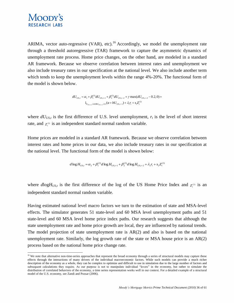
Moody’s Mortgage Metrics Prime Technical Document (2010) 36 of 61
ARIMA, vector auto-regressive (VAR), etc).16
Accordingly, we model the unemployment rate
through a threshold autoregressive (TAR) framework to capture the asymmetric dynamics of
unemployment rate process. Home price changes, on the other hand, are modeled in a standard
AR framework. Because we observe correlation between interest rates and unemployment we
also include treasury rates in our specification at the national level. We also include another term
which tends to keep the unemployment levels within the range 4%-20%. The functional form of
the model is shown below.
where dUUS,t is the first difference of U.S. level unemployment, rt is the level of short interest
rate, and is an independent standard normal random variable.
Home prices are modeled in a standard AR framework. Because we observe correlation between
interest rates and home prices in our data, we also include treasury rates in our specification at
the national level. The functional form of the model is shown below:
where dlogHUS,t is the first difference of the log of the US Home Price Index and is an
independent standard normal random variable.
Having estimated national level macro factors we turn to the estimation of state and MSA-level
effects. The simulator generates 51 state-level and 60 MSA level unemployment paths and 51
state-level and 60 MSA level home price index paths. Our research suggests that although the
state unemployment rate and home price growth are local, they are influenced by national trends.
The model projection of state unemployment rate is AR(2) and also is based on the national
unemployment rate. Similarly, the log growth rate of the state or MSA house price is an AR(2)
process based on the national home price change rate.
16 We note that alternative non-time-series approaches that represent the broad economy through a series of structural models may capture these
effects through the interactions of many drivers of the individual macroeconomic factors. While such models can provide a much richer description of the economy as a whole, they can be complex to optimize and difficult to use in simulation due to the large number of factors and
subsequent calculations they require. As our purpose is not to manipulate individual “levers” in the economy, but rather to simulate the
distribution of correlated behaviors of the economy, a time series representation works well in our context. For a detailed example of a structural model of the U.S. economy, see Zandi and Pozsar (2006).
, 1 , 1
(1) (1)
, 1 1 , 1 2 , 2 , 2
(1)
4 11 , 1 1 1
max( 0.2,0)
1 ( )US t US t
US t US t US t US t
U ORU US t t t
dU dU dU dU
a bU r s Z
)1(
tZ
)2(
222,
)2(
21,
)2(
12, logloglog tttUStUStUS ZsrHdHdHd
(2)
tZ

Moody’s Mortgage Metrics Prime Technical Document (2010) 37 of 61
where is the unemployment rate in the region (state/MSA) at time t and is the
HPI in the region at time t.
Box 4 describes how these models are used in simulation. Note that we do not model correlation
between home price changes in different states or MSAs explicitly through, say, a correlation
matrix. Correlation enters into the models due to their common dependence on the national level.
2.12.3 Freddie Mac (FHLMC) mortgage rate
Calculation of the spread-related factors in our models requires knowledge of the prime
mortgage market rate, F(t). We use the Freddie Mac 30 year commitment rate as a proxy for the
prime market rate. This rate is modeled as:
, 1 , 1
(1) (1)
, 1 1 , 1 2 , 2 ,
(1)
4 11 , 1 1
ˆ ˆˆ ˆ
ˆˆ1 ( )region t region t
region t region t region t U US t
U ORU region t t
dU dU dU dU
a bU s Z
)2(
2,2,
)2(
21,
)2(
12,ˆˆlogˆlogˆlogˆˆlog ttUSHtregiontregiontregion ZsHdHdHdHd
,region tU ,region tH
1 2 3 4 1 5 210 F
t t t t t t f tdF dCMT ds dY dF dF Z
Box 4: Simulating HPA and Unemployment
Simulating an economic scenario for home price changes involves the following steps:
1. Simulate national level HPA using:
a. the simulated value of interest rates (from Box 3)
b. lagged values of national HPA (simulated or observed, see section 2.16.2)
c. a random shock;
2. For each state or MSA (local region)
a. Simulating local region home price changes using:
i. the previous values of the local region changes (simulated or observed, see
section 2.16.2))
ii. the national level of HPA (from step 1, above)
iii. the interest rate
iv. a random shock.
Unemployment is simulated the same way, except we replace the home price with the level of
unemployment.

Moody’s Mortgage Metrics Prime Technical Document (2010) 38 of 61
where CMT10 is the 10 year treasury rate, st is the spread between the 6 month LIBOR rate and
the 6 month treasury rate, Yt is the difference between the 10 year treasury rate and the 6 month
treasury rate, which is a measure of the slope of the yield curve, and dFt-1 and dFt-2 are the lagged
changes in the mortgage rate, F.
2.13 Incorporating delinquencies and realized pool performance
Moody’s Mortgage Metrics Prime can be used to analyze the loss distribution not only of new
pools, but also of seasoned pools for which historical performance information is available. For a
seasoned pool, the losses consist of two components – those that have already been realized since
the pool’s inception or closing date (historical), and those that are projected from today
(simulation). While there is only one historical realization up through the current period, we
generate 10,000 economic simulations for periods after the current period to arrive at a
distribution of future or projected losses.
Seasoned pools offer additional information for predicting lifetime losses. As a pool seasons, we
can observe the following:
Updated value of the loan balance, including any curtailment;
Up-to-date delinquency status (Current, 30DPD, 60DPD, 90DPD) for each loan in the
pool ;
Which loans have already prepaid or defaulted; and
For defaulted loans, the actual loss in cases where the losses have been realized.
We estimated the hazard rates for prepayment and default models described in Section 2.5 using
a sample consisting of current and delinquent loans.
However, when we apply the models to seasoned loans, we know their payment status, and this
information helps to predict future default or prepayment. For example, a loan that is current is
less likely to default relative to the general population, which includes both, current and
delinquent loans; whereas a loan that is 90 days past due is more likely to default relative to the
general population.
Accordingly, for seasoned loans, instead of using the sample wide (unconditional) hazard rate
baselines to predict default and prepayment we use a different baseline hazard rate for each

Moody’s Mortgage Metrics Prime Technical Document (2010) 39 of 61
delinquency status. These delinquency-specific baseline hazard rates are scaled versions of the
sample-wide hazard rates.
It is useful to consider why the realized loan performance might be different than the model’s
prediction. The loan-level models are developed based on loan and borrower attributes
observable in our data set. Hence the prediction of our model will be an unbiased estimate of a
pool’s performance for all cases in which the unobserved attributes of the pool are similar to
those of the general population. However, if the loans in a given pool were selected according to
some criteria that are unobservable to us but different from the general population, our
predictions could be systematically biased for that pool. For example, a pool of loans made to
high net worth individuals might have a lower default rate than our model would predict because
of an attribute unobservable to us, namely, the total wealth of the borrowers.
We use the differences in predicted versus actual loan performance as of the current date to
adjust our models in real time to account for pool-specific default and prepayment drivers that
are not observable. Specifically, after selecting an appropriate baseline for a loan we then scale
this baseline to account for differences in predicted versus observed performance to date. The
scaling factor is chosen so that the predicted 5 year default and prepayment rates for a group of
loans of the same delinquency status match closely their realized counterparts.
We estimate the scaling parameters as follows: we predict loan performance as of the current
date for the current loans using the realized economy from loan origination to the present date as
the input for the macro factors for the model. We calculate the difference between the predicted
and actual realized values. We then scale the baseline hazard rate to reduce the difference. We
repeat this process, adjusting the scaling factor until we find a value that sets the predicted rate
equal to the realized rate. We use a scaling scheme that naturally bounds the default and
prepayment rates between 0 and 1.
When analyzing a seasoned pool, we use the realized defaults, prepayments and actual losses, if
available, to calculate the performance of the pool to-date, and only use simulations to predict
the performance of the pool going forward.
Actual losses (severities) are often realized 12 to 18 months after default. In some cases, trustees
may never report the actual losses. To calculate performance to-date, we use actual losses if they
are available, and otherwise use our severity model to estimate the loss.

Moody’s Mortgage Metrics Prime Technical Document (2010) 40 of 61
2.14 Enhancements based on expert judgment
Ideally, historical data used for calibrating the econometric models would be both fully
descriptive of the underlying process and complete. In reality, this is seldom the case. The pace
of innovation in the mortgage market has been rapid. New mortgage products, new underwriting
practices and new approval technology all suggest behaviors that may not be fully captured in
the historical data.
Because of this limitation, we augment our statistical modeling with detailed discussions with
RMBS analysts and other market participants. Our goal is to ensure that we capture newer
developments in the market as they manifest themselves in prime mortgage behavior particularly
if historical data are not sufficient to model these phenomena.
Our goal in incorporating qualitative analysis is to augment the models rather than to introduce
arbitrary behavior. When there are neither sufficient data nor standardized reporting to permit
quantitative estimation, we incorporate appropriate expert judgment to improve our model. In
general, these adjustments serve to “fill in the gaps” in the relationships in our statistical analysis.
These gaps are typically due to either the newness of some aspect of a market or economic states
of the world that have not yet manifested themselves in the historical record.
We try to make these adjustments to our models in ways that are consistent with our modeling
framework. For example, when we introduce augmented data (certain property types, certain
documentation types, etc.) for which historical data are generally unavailable, we do so by
introducing adjustments to our default model directly, rather than adding “hits” to expected loss.
Furthermore, upon augmenting the models to reflect a specific characteristic of the market, we
perform extensive validation to ensure that the results generated by the model following the
enhancements are intuitive.
We use such adjustments sparingly, but include them when they are needed. Some examples of
these adjustments are:
The introduction of additional documentation (doc) type codes to permit better granularity
for doc type;
Sensitivity of models to unemployment levels outside of the range of the historical data; and
Frailty parameters.

Moody’s Mortgage Metrics Prime Technical Document (2010) 41 of 61
In addition, due to the difficulty in calibrating a model to properly predict extreme events, many
of which are not present in the historical data, we also use expert judgment in calibrating the
extreme loss levels predicted by the model.
2.15 Frailty
While we endeavor to capture known risk factors through either statistical estimation or expert
judgment, it is inevitable that some unknown factors and some known but impractical to quantify
factors can influence default behavior. A recent stream of research in the corporate default
literature (c.f., Duffie, et al., 2009) has begun to explore models that expressly accommodate
such latent frailty phenomena. The term frailty has been adopted from the health sciences
literature where similar approaches are used to examine patient mortality.
Frailty need not relate only to macro-economic shocks. As a hypothetical example, consider how
the adoption of a defective fraud-detection system for mortgage underwriting might impact
default rates. Now, all underwriters using the system may experience higher default rates as a
result: they will experience correlated defaults that are explained by the common use of this
system. A more realistic example would be an earthquake or terrorist attack. While such factors
clearly induce correlation among mortgage defaults, it is unlikely that any model would include
these factors, a priori, and there are clearly a very large number of such factors, the impact of
which would only be realized ex post.
The estimation techniques for frailty models are involved and typically require long time series.
As a first step in including frailty in our models, we have implemented a simpler framework,
similar to many parametric frameworks for imposing correlated defaults. In order to
parameterize the model, we used a combination of expert judgment and empirical analysis.
The frailty component of the model works as follows: For each loan i the default model predicts
a default probability, di. A correlation between the default events of different loans is introduced

Moody’s Mortgage Metrics Prime Technical Document (2010) 42 of 61
by the generation of a series of correlated Uniform [0, 1] variables, Xi, for each loan (see
equation below). Default occurs for loan i if Xi is less than the loan’s default probability, di.
( 1 )
where
(.) cumulative normal distribution
is the correlation
, are independent standard normals
i i
i
X N s
N
s
Thus, in addition to the correlation in default rates induced by the dependence of default rates on
common interest rates and local macro-economic factors (themselves correlated with the national
level), the default events of all loans are also correlated through their dependence on the latent
frailty factor.
Note that the estimation techniques for formal frailty models are involved and typically require
long time series. Our implementation uses a simpler framework, and is similar to many
parametric frameworks used for modeling correlated defaults. We estimate our frailty model,
using a combination of expert judgment and empirical analysis.
2.16 Estimating Loss Distribution using Monte Carlo simulation
In this section, we describe the simulation module that Moody’s Mortgage Metrics Prime uses to
generate the states of the economy used by the other models in estimating default probably,
prepayment probability, and severity. The engine uses a full multi-step Monte Carlo simulation
to estimate the collateral loss distribution.
2.16.1 Estimation of the loss distribution
We estimate the collateral loss distribution in the following way: we simulate macro-economic
variables for 10,000 different economic scenarios, quarterly, over a ten year horizon. For each
simulated economy, we determine if and when a loan defaults or prepays and the loss incurred
on the loan if it defaults. For each economy, we add the dollar amounts of the losses on all the
loans in the portfolio to arrive at the dollar amount of loss for the pool. This quantity is divided
by the notional balance of the pool to obtain the fractional loss (henceforth, referred to as the loss)
for the pool. When this process is repeated for each of the 10,000 simulated economies, we get a

Moody’s Mortgage Metrics Prime Technical Document (2010) 43 of 61
histogram of these 10,000 losses and, thus, the empirical loss distribution. This distribution for
one of the pools is shown below in Figure 9. The graphic is taken from one of the reports that the
software produces during its analysis.
Figure 9: Portfolio loss distribution
2.16.2 The use of lagged values during simulation
Some of the macro-factor models use lagged values of the same or other variables as explanatory
variables. For example, our current value of Home Price Appreciation (HPA) is a function of the
two previous lagged values of the variable. When lagged values are required to simulate the
current value of a macro factor, we use observed data (i.e., actual past HPA, interest rates and
unemployment) when it is available. Since the models only use two lags, actual data can only be
used, at most, for the first two quarters of the simulation. To simulate the macro variables further
out into the future, we use simulated values from previous time steps as the lagged values. We
illustrate how we use actual versus simulated values in the simulation by considering how HPA
is calculated for the first four quarters of the simulation. Recall that the current value of HPA is
modeled as a function of its two previous lagged values, in addition to other factors. Assume that

Moody’s Mortgage Metrics Prime Technical Document (2010) 44 of 61
the simulation is starting 2010Q3 and that we have all historical values of HPA up to and
including 2010Q3 as reported by Moody’s Economy.com.
Table 2 shows how the simulation would proceed along a particular path. We denote the
simulated values with a superscript “s” (s). For the first quarter forward, we run the simulation
and compute HPA 2010Q4s. Since HPA depends on its own two lags, we use the actual HPA
values for 2010Q3 and 2010Q2 to compute 2010Q4. Similarly to compute HPA 2011Q1s, we use
the actual HPA value of 2010Q3 and simulated HPA value 2010Q4s.
Table 2: Example of HPA simulation
Simulation period Lag t-2 Lag t-1 Scenario value t
1 – 2010Q4 HPA 2010Q2 HPA 2010Q3 HPA 2010Q4 s
2 – 2011Q1 HPA 2010Q3 HPA 2010Q4 s HPA 2011Q1
s
3 – 2011Q2 HPA 2010Q4s HPA 2011Q1
s HPA 2011Q2
s
4 – 2011Q3 HPA 2011Q1 s HPA 2011Q2
s HPA 2011Q3
s
2.17 Analyzing the Loss Distribution
In addition to determining the expected loss for the entire mortgage pool, it is sometimes useful
to consider the expected loss above or below a specific point on a distribution. In traditional risk
management, these portions are commonly characterized as the value at risk (VaR) and expected
shortfall or expected tail risk (ETR). In a structured finance setting, variations on these quantities
are typically thought of as tranches.
A tranche defines an interval of the loss distribution bounded on the bottom by an attachment
point and above by a detachment point. A specific tranche suffers no losses if the portfolio losses
are less than the attachment point for the tranche. The tranche is, however, exposed to all
portfolio losses beyond the level of the attachment point.
Since the loss distribution describes the probability associated with each level of loss on the
portfolio, the expected loss for a particular tranche is readily calculated as the probability
weighted percentage losses to the tranche.
Since agency ratings can also be characterized using (idealized) expected losses or expected
default rates, it is convenient to compute the rating category associated with various points on the
loss distribution. These provide information about the tail risk in the mortgage pool. In the case
of the expected default rate, the attachment point is simply the quantile of the distribution

Moody’s Mortgage Metrics Prime Technical Document (2010) 45 of 61
associated with the target default rate or the VaR. In the case of expected losses, the calculations
are a bit more involved but the logic is similar. We describe these calculations in the remainder
of this section.
Importantly, the expected loss on a tranche is typically a function not only of losses on the
underlying portfolio of mortgages, but also of the manner in which the various mortgage cash
flows (e.g., interest spread, recoveries, etc.) are apportioned in the transaction as prescribed by
the cash flow waterfall. The analysis below assumes a simple cash flow waterfall where cash
flows are apportioned strictly by tranche seniority. While this analysis is suggestive of loss levels
on tranches in general, it applies most closely to sequential pay structure or synthetic structure.
(For cashflow transactions, various triggers, the use of excess spread and so forth can materially
change the risk of specific tranches.)
2.17.1 Expected loss for a tranche17
We use the following notation for our derivations:
L is a portfolio loss level
FL(L) is the cumulative distribution function (CDF) of L
fL(L) is the corresponding probability density function (pdf).
We now define the expected loss for a tranche with an attachment point of A and a detachment
point of D. Whenever the pool experiences a loss (L) less than A, the tranche experiences zero
loss. Whenever the pool experiences a loss greater than D, the tranche is completely wiped out,
i.e., it experiences its maximum loss, D – A. When the collateral losses are greater than A but less
than D, the tranche loss rate increases linearly from 0 at A to 100% at D. For this region of
collateral loss, we get:
L A
Tranche loss rateD A
In practice, the exact distribution of the losses is not known. However, Moody’s Mortgage
Metrics Prime provides a simulation-based estimate of the loss distribution which can be used to
readily compute tranche ELs.
17 This section is adapted from Das and Stein (2010) which also contains more detailed analysis of the properties of different tranching approaches.

Moody’s Mortgage Metrics Prime Technical Document (2010) 46 of 61
The expected loss of this tranche can be expressed using the pdf of the loss distribution and the
tranche loss as
1
min ,1 ( )L
A
L ATranche EL f L dL
D A
Given a target EL for a specific credit grade, it is possible to assign a credit grade to any tranche
in a capital structure, based on the EL for the tranche. For example, Table 3 below shows
Moody’s idealized EL values for different credit ratings, based on 10-year horizons, though any
set of EL targets could be used.
Table 3: Moody’s idealized (target) Expected Losses by Rating
Rating EL (%)
Aaa 0.0055
Aa1 0.055
Aa2 0.11
Aa3 0.22
A1 0.385
A2 0.66
A3 0.99
Baa1 1.43
Baa2 1.98
Baa3 3.355
Ba1 5.17
Ba2 7.425
Ba3 9.713
The minimum tranche credit enhancements needed to attain a specific rating grade can be
calculated numerically.18
The process starts from the highest rated tranche and proceeds to the
lowest rated tranche as follows. First, the Aaa level is determined. The detachment point for Aaa
is 100%, and the idealized EL is 0.55bps (Table 3). Therefore, the above formula for tranche EL,
with pool loss expressed as percent, becomes
18 Note that these level approximations are not equivalent to ratings for a variety of reasons.
Moody’s Mortgage Metrics Prime Technical Document (2010) 47 of 61
1
min ( ) .0000551
CE L
A
L AAaa A f L dL
A
Although this equation has no closed-form solution, we can easily solve iteratively for the lowest
value of A by reducing A from 1 until the above inequality is violated. The value of A which
solves the above equation is the Aaa credit enhancement, AaaCE.
The detachment point for Aa1 is equal to the Aaa attachment point, and its idealized EL is 5.5
bps. So, we can again obtain the Aa1 attachment point by solving for value of B that solves the
expression below for the Aa1 tranche
1
1 min min ,1 ( ) .00055CE L
CEB
L BAa B f L dL
Aaa B
This process is repeated until all tranche levels are determined.
Some properties of the losses experienced by tranches are worth noting. The same attachment
point can result in quite different losses on a tranche depending on the size of the tranche (the
location of the detachment point). For this reason, “thin tranches” tend to be much riskier than
thicker tranches even when both have the same level of subordination (the same attachment
point). Also, it is not guaranteed that an attachment and detachment point can be found for target
EL. In some cases, the shape of the distribution is such that some ELs cannot be achieved
through subordination without reducing the size of (or eliminating) tranches above.
3 DATA
We use data from several different sources for our analysis
A database of individual mortgages containing loan-by-loan characteristics and
performance provided by a leading RMBS originator;
a database constructed based on data files from RMBS trustees which was downloaded
from trustee sites;
historical macroeconomic data and forecasts from Moody’s Economy.com;
lifetime loss estimates for RMBS asset pools from Moody’s RMBS surveillance group;

Moody’s Mortgage Metrics Prime Technical Document (2010) 48 of 61
summary statistics published in various academic and industry articles
We obtained economic data, going back to 1980, from Moody’s Economy.Com (MEDC), which
receives data from various sources. For example, the MEDC unemployment rate data are
collected from the US Bureau of Labor Statistics. The home price index comes from the National
Association of Realtors (NAR) and is the median home price of existing single family homes
sold in each quarter. We use the unemployment rate and the home price index at the national,
state, and Metropolitan Statistical Area (MSA) level. Given the large number of MSAs, we
include 60 of the most common MSAs. .
Our primary source of loan-specific information is a prime mortgage loan database provided by a
large mortgage originator. This dataset contains a sample of hundreds of thousands of loans
originated as far back as 1998 with good data density from 2002 onwards. Since the data was
provided by a single originator, we tested it extensively for representativeness and completeness
to ensure our model did not appear to be biased towards the idiosyncrasies of this particular
sample. In general we found that from a statistical perspective the data are similar to data
reported in other studies and to other data sets that we examined, both in terms of the frequency
distributions of the independent variables (loan characteristics, etc.) and in terms of the timing,
frequency and levels of the default and prepayment.
We further perform out-of-sample tests of our models using a second data set comprised of a
broad cross section of both individual loans and RMBS pools downloaded from trustee sites of
many trustees. Here again, the models appear to perform well regardless of whether they are
tested on the original development sample or the sample composed of loans from many different
originators.
3.1 Data mapping and cleaning
In many cases, financial institutions maintain data sets to support business functions and not to
develop quantitative models. As a result, data quality that is appropriate for their business
applications may not be adequate for modeling. Accordingly, we perform a series of data
standardization and mapping processes to address several data issues.
The data-refinement process begins with a mapping of provider fields to a standard format and
standard definitions. When we first receive data, either from trustees or from an originator, we
try to work with the provider to determine how best to map their data fields to the common
definitions we use. As part of the mapping, we examine the granularity of the fields based on the
providers’ definitions. For example, some contributors maintain only three categories of

Moody’s Mortgage Metrics Prime Technical Document (2010) 49 of 61
documentation type while others have as many as twelve. In order to have a common data
structure across all observations in our data set, we re-classify entries in such fields to a common
number of categories that still provides sufficient discriminatory power.
Once the data have been mapped to a common format, we perform a formal data standardization
and error trapping process in three steps that progressively deal with increasingly subtle data
errors:
First, we eliminate the obvious typographical errors. We do this by flagging records where
values of any field appear erroneous using a rule-base that we have created. The rule-base is
tailored to individual data contributors. Where possible we also create rules to correct these
errors. For example, a FICO score of 7200 may be converted to 720 where it is obvious that this
is the intended value. However, a FICO of 23 or 2300 is erased and labeled “unknown” since it is
not obvious what the corresponding correct value is. (23, 2300, and 230 are outside of the valid
range of FICO.)
Next, we identify errors using business rules that flag values of certain fields that seem to be in
conflict with basic business or accounting logic. For example, we verify that a loan’s combined
LTV (CLTV) is at least as great as its LTV and that the remaining term on a loan is no longer
than its original term. Where possible, we correct errors by recalculating the incorrect fields
using information from other fields in the record.
Finally, we use statistical anomaly detection techniques to identify potential errors in the data.
We develop univariate and multivariate relationships between fields in the data set and then use
these relationships to flag observations where predictions from the statistical relationships are
outside of the expected range. We then investigate whether these outliers are legitimate
observations or are bad data that should be removed from the sample.
In each level of refinement, we apply rules that we have developed in conjunction with data
providers themselves or with our own analysts and researchers.
3.2 Sample descriptive statistics
Since the data used for fitting our models are provided by a single originator, we test it
extensively for representativeness and completeness to ensure our model is not somehow biased
toward the idiosyncrasies of this particular originator. We find that the data set is similar to those
used in other studies and to other data sets we examined, both in terms of the distribution of loan
characteristics as well as in terms of loan performance. Figure 10 shows the distribution of our

Moody’s Mortgage Metrics Prime Technical Document (2010) 50 of 61
data along various dimensions. Our analysis suggests that this data set is representative of the
population of loans in the prime mortgage market and that no key segment of the market appears
to be missing in our data set.
Figure 10: Data distributions by loan attributes
4 MODEL VALIDATION
We discuss the validation tests performed after we calibrated the different models for loan
performance and for different macro factors. Validation is an important step in the development
process for a model used for commercial applications, and we spent a significant amount of time
on the validation process.
We performed two broad types of validation tests:

Moody’s Mortgage Metrics Prime Technical Document (2010) 51 of 61
Sensitivity tests: These tests examine whether the sensitivity of losses to changes in
individual factors (such as FICO or LTV) predicted by the model is in accord with
economic intuition.
Prediction tests: These tests examine whether the predicted loss performance of the
model is consistent with realized values or other benchmarks. These include tests of the
discriminatory power of models as well as tests of the predicted levels of default.
4.1 Sensitivity Tests
We examine the sensitivity of pool-level losses to key loan attributes and macro factors to ensure
they are consistent with economic intuition.
Figure 10 shows an example of the sensitivity analysis performed. This figure illustrates how the
pool-level expected loss varies with changes in national housing prices. As shown in the figure,
losses increase as HPA decreases, which suggests that predictions made by M3 Prime is
consistent with economic reasoning.
The pool used for this example was a seasoned pool originated in 2006Q1. The average FICO
score was 750 and the average CLTV was approximately 70%. The change in housing prices
shown in this figure is the cumulative change over the first two years of the simulation. The
sensitivity is calculated as follows:
o The simulation started at time t (2010Q1), with the macro factors and loan-specific attributes
evolving according to the models described in earlier sections.
o At time t+2 years, we record the cumulative home price appreciation along each path from t
to t+2, and group paths with similar HPA values into n bins. For this example, we segment
home price movements into n=12 distinct bins.
o At the end of the simulation period, which is t+10 years, we compute the pool-level losses
for each path, average these losses across all paths belonging to a particular bin, and report
these losses as the loss corresponding to a particular range of HPA values as shown in Figure
9. That is, the loss for each bin is E[pool loss|HPChange in HPArange(j)], where
HPArange(j) is the range of 2-year cumulative HPA values corresponding to bin j.

Moody’s Mortgage Metrics Prime Technical Document (2010) 52 of 61
Since we are using the results of the simulation to compute sensitivity to HPA, all variables other
than HPA vary according to the models specified earlier. We use this approach to calculate
sensitivity analysis as there are significant interaction effects between HPA and other macro
factors as well as loan attributes on the pool loss, and the simulation approach provides a natural
way of accounting for these interaction effects. Accordingly, our measure of sensitivity of pool-
level expected losses to change in HPA is
𝑠𝑒𝑛𝑠𝑖𝑡𝑖𝑣𝑖𝑡𝑦 = 𝛥𝐸[𝑝𝑜𝑜𝑙 𝑙𝑜𝑠𝑠𝑒𝑠|𝐻𝑃𝐴]
𝛥𝐻𝑃𝐴
Sensitivity analysis for other variables of interest is performed in a similar manner. Another
example of sensitivity analysis is provided in Figure 11. This figure summarizes the sensitivity
of pool-level losses to a loan attribute, namely, CLTV. The expected loss for each CLTV bin is
calculated using an approach similar to that described earlier, except that the grouping is now
based on loans that have similar CLTV at origination and averaging is done over all paths.
Recall that the model simulates losses on a loan-by-loan basis, which facilitates analyzing how
different sub-groups of loans perform. As seen from the figure, the expected losses increase with
CLTV, which again suggests that the predictions of the model are consistent with economic
reasoning. Since the averages calculated for sparsely populated bins (less than 100 points) are
likely to have large variance, we display conditional averages for such bins using a dotted instead
of a solid background. This can be seen in Figure 11.
We described how we use sensitivity analysis for model validation. Because users of the model
also find it useful to examine such sensitivities, either to better understand how the model
behaves or to conduct scenario analysis, we have also implemented a number of analytic and
graphical reports to characterize the behavior of the model for several key macro factors and loan
attributes. In fact, Figures 10 and 11 are directly taken from the standard output the portfolio
analysis software.

Moody’s Mortgage Metrics Prime Technical Document (2010) 53 of 61
Figure 11: Model sensitivity to macroeconomic levels
Figure 12: Model Sensitivity to Loan-specific Factors Levels
7.5% &
higher
7.5% to
2.5%
2.5% to
0.0%
0.0% to
-2.5%
-2.5% to
-5.0%
-5.0% to
-7.5%
-7.5% to -
10.0%
-10.0%
to -
12.5%
-12.5%
to -
15.0%
-15.0%
to -
20.0%
-20.0%
to -
25.0%
-25.0%
& lower
Sparse data 0.00 0.00 0.00 0.00 0.00 0.00 0.00 0.00 0.00 0.00 0.00 0.00
Fuller data 8.94 10.51 11.37 11.91 12.51 13.24 13.94 14.63 15.40 16.53 18.07 20.07
0.00
5.00
10.00
15.00
20.00
25.00
EL
Change in National HP
60 & lower
60 to 70
70 to 80
80 to 85
85 to 90
90 to 95
95 to 100
100 to 105
105 & higher
Sparse data 0.00 0.00 0.00 0.00 0.00 0.00 0.00 0.00 0.00
Fuller data 4.29 7.34 10.08 14.85 16.61 17.91 17.66 0.00 0.00
0.002.004.006.008.00
10.0012.0014.0016.0018.0020.00
Mean
loan
EL
per b
ucket
CLTV

Moody’s Mortgage Metrics Prime Technical Document (2010) 54 of 61
4.2 Predicting defaults for known macroeconomic paths
The sensitivity tests described in the previous section are conducted to examine whether the
variation in model prediction because of a variation in macro factors or loan attributes is
consistent with economic reasoning. We now examine whether the level of default rates
predicted is consistent with realized values.
Our portfolio tool was developed to estimate the distribution of pool-level losses. This
distribution is generated by first simulating different states of the economy and then predicting
the losses conditional on the states of the economy to generate a distribution of losses.
Since our effort focuses on predicting defaults conditional on the states of economy, we validate
the predictive capability of the model by examining whether predicted default levels match
realized levels, assuming we know the actual state of the economy, which we do for historical
paths.
We conduct our test using historical values of macroeconomic factors to predict defaults at
different points in time and compare these predictions to the realized levels of defaults.
The procedure we use is detailed below:
1. Start in a month t and create a cohort of loans outstanding in month t
a. For T quarters into the future, run the default model and the prepayment
model to estimate the one-month default probability and prepayment
probability for each loan for each month from time t to t+T. At the end of
month t+T, calculate the T-month cumulative predicted default probability by
compounding the one-month default and one-month prepayment probabilities.
b. Calculate the pool-level cumulative default probability as the average default
probability across all loans in the pool
2. Compare the predicted cumulative default probability to the realized default rate over
the same period
3. Repeat Steps 1, 2 and 3 for each month in the data set (except for the last T months,
as we will not have T-month-ahead realized default rates for these months)
We perform this validation exercise on both, data from the development sample (base sample)
updated to include the most recent out-of-sample period as well as data from a separate sample

Moody’s Mortgage Metrics Prime Technical Document (2010) 55 of 61
of recent vintage mortgage pools from a diverse set of originators that were collected from
RMBS trustees (trustee data set). Samples of the results are presented below in Figure 13 and
Figure 14, respectively. These are representative of the general results we observed for various
subsets of the data (with the exception of a few cases which we discuss in more detail below).
Figure 13: Realized and predicted default rates with confidence bounds – base sample
Figure 14: Realized and predicted default rates with confidence bounds – Trustee data set

Moody’s Mortgage Metrics Prime Technical Document (2010) 56 of 61
Figure 13 shows the 36 month default rate (i.e., T= 36 months) for all loans in the base data set
as a function of calendar time. The realized default rate is shown in solid line, the model forecast
is shown in dashed line and the 95% confidence bounds are shown in dotted lines. Figure 14
shows similar information for the loans not used to develop the model. These are available for a
shorter observation period, but nonetheless provide evidence that the models perform well on
loans from a wide variety of originators.
In considering these exhibits, a few features are worth noting. First, the observed data represents
actual performance, net of the effects of Home Affordable Modification Program (HAMP), while
the model output is meant to be a “pure-play” on loan quality and economic environment.
Therefore, we should expect systematic deviations between the observed and predicted values
during the HAMP period and find that the models’ estimates are higher than observed values for
the last part of the sample period.
Second, the model’s predictions (dashed line) appear to be a “stair-step” plot in comparison to
the relatively smooth plot for realized defaults. This is because the macro data used as an input to
the predictions is only updated quarterly, whereas realized defaults are available monthly. The
small variation in month-to-month predicted defaults is primarily because of the relatively minor
effect of loans leaving the sample due to maturity or prepayment.
To gain more insight into the behavior of the models in different settings, we examine the
performance of our model for different types of loans. We repeat our analysis on various sub-
groups of loans, such as: ARM/Fixed, High/Medium/Low LTV, different states, different loan
margins, large/small loan amount. In general, the results are consistent with those shown above,
though, as expected, the confidence bounds widen as the number of loans used in the test pool
shrinks because of subsetting.
Unsurprisingly, our model cannot match the realized performance of pools that are affected by a
unique pool-specific shock. For example, borrowers in the State of New York were particularly
affected by the events of 9/11. Figure 14 plots default information for a pool of NY loans in our
data set. As seen in Figure 15, realized default rates increased markedly for a period following
9/11. Since our model does not explicitly account for terrorist attacks, our prediction
significantly under estimates defaults for about two years following the attack. However, as the
economic impact of 9/11 abates, we again find good agreement between predicted and realized
default rates.

Moody’s Mortgage Metrics Prime Technical Document (2010) 57 of 61
Figure 15: Realized and predicted default rates for all NY state loans in our data set
4.3 Comparing model predictions to analyst estimates
Finally, we compare the model’s loss performance estimates with those developed by analysts.
The comparisons are made for seasoned pools. For each mortgage pool, the portfolio tool
estimates the cumulative expected losses for a 10-year period, starting from the deal origination
date. For seasoned pools, the model uses the actual historical values of economic factors to
predict pool performance from origination to the current date, and then uses simulations to
predict additional future losses from the current date to the end of the 10-year period used for the
analysis. The model’s estimates are compared with those developed by the RMBS surveillance
group at Moody’s Investors Service. This group’s estimates are based on actual pool-level losses
realized to-date plus an estimate of future losses. Their estimate of future losses is based on their
expert judgment as well as on assumptions of appropriate roll-rates for different statuses of the
loans (e.g., 60+ delinquent and 90+ delinquent). Note that since the model’s estimates do not
include adjustments for HAMP or other government programs, the analysts’ estimates were
adjusted to be net of HAMP as well.

Moody’s Mortgage Metrics Prime Technical Document (2010) 58 of 61
We report results of the comparison in Table 4for a set of mortgage pools originated at different
points in time, starting from 2006Q1 to 2007Q4. For each quarter, we report the average pool-
level losses estimated by the model versus those estimated by the analysts. The average is
calculated across all the pools in our sample for the particular quarter of deal closing. These tests
were performed based on analysis done in the beginning of the second quarter of 2010.
Table 4: A comparison of the average expected loss over prime pools: M3 Prime Vs. Surveillance
Comparison Date Moody’s Mortgage
Metrics Prime estimates
MIS RMBS Surveillance
Group estimates
2006Q1 8.4 8.3
2006Q2 9.6 9.3
2006Q3 9.1 8.9
2006Q4 8.7 8.5
2007Q1 13.0 12.4
2007Q2 14.1 13.7
2007Q3 13.7 12.6
2007Q4 15.7 15.3
We also note that the pool estimates demonstrated high correlations with analysts’ estimates at
the individual pool level as well as the vintage level. These results suggest that the model’s
predictions are consistent with those developed by analysts.
5 CONCLUSIONS
In this paper, we have described some of the details of the Moody’s Mortgage Metrics Prime
models. This suite of quantitative models is integrated into an analytic portfolio tool for
assessing the risk of prime residential mortgage portfolios. The tool calculates, in a correlated
fashion, the default, prepayment and severity of (typically thousands of) individual mortgages in
a pool and then aggregates these risks taking into account the loan-level characteristics as well as
macroeconomic variables.
Moody’s Mortgage Metrics Prime is a quasi-structural model of mortgage portfolio loss: the
individual drivers of losses are correlated but are treated as unique processes, and these processes
are integrated in an economically coherent manner so that both the behavior and the results of the
analytics are economically rational.
Our research has yielded a number of stylized facts. Firstly, our results suggest that there does
not appear to be a single factor (or two) that can in general explain the losses on mortgages and

Moody’s Mortgage Metrics Prime Technical Document (2010) 59 of 61
mortgage pools; instead, we find that the recent industry trend towards “layered risk” analysis is
justified and in fact required. As a result, we find that it is far more effective to model
prepayment, default and severity at the loan level if the goal is to accurately capture the loss
behavior of large pools of mortgages, particularly when the assets in the pools are distributed
heterogeneously. Doing so also reveals that prepayment rates can at times be the dominant effect
in determining the distribution of pool losses and that without adequately analyzing prepayment
processes, losses are difficult to understand over the medium term.
We also find evidence that all three of the underlying processes that drive losses appear to be
correlated through their joint dependence on economic factors such as the levels of interest rates
and local home prices (there is a weaker dependence of some processes on local unemployment
rates). This dependence in turn induces correlation among the loans in a portfolio which must be
modeled.
Though the results of our analysis and validation are encouraging, this should not be taken to
imply that the models cannot be further improved. Indeed, research on our next generation of
models is already underway. While we feel that the Moody’s Mortgage Metrics Prime approach
represents a useful tool for analyzing mortgage pool losses, we are also quite cognizant of the
limitations of the model. We expect to introduce refinements to various aspects of the models as
our data set continues to grow and our research reveals additional structure in mortgage behavior.
This underscores the spirit in which the model should be used: as an input to rather than a
substitute for a rigorous analytic process. As an input to an analytic process, the approach can
enhance users’ understanding of the risks in mortgage portfolios they evaluate.
6 REFERENCES Acharya, V., B. Sreedhar, and A. Srinivasan, 2004, Understanding the Recovery Rates on
Defaulted Securities, and references therein.
Bolder, D. J., 2001, Affine Term-Structure Models: Theory and Implementation, Working paper,
Bank of Canada, 2001-15.
Breslow, N. E , 1974, Covariance Analysis of Censored Survival Data, Biometrics 30, 89-99.
Cox, C.J., J.E. Ingersoll, and Jr., S.A. Ross, 1985, A Theory of the Term Structure of Interest
Rates, Econometrica, 53 (2), 385-408.

Moody’s Mortgage Metrics Prime Technical Document (2010) 60 of 61
Cox, D. R.,1972, Regression Models and Life Tables (with discussion), Journal of the Royal
Statistical Society B34, 187-220.
Das, A. and R. Stein, 2010, Differences in Tranching Methods: Some Results and Implications,
Working Paper, Moody’s Research Labs.
Dwyer, Douglas W., and Roger M. Stein, 2004, Moody’s KMV RiskCalc v. 3.1 technical
document, New York: Moody’s KMV.
Duffie, D., A. Eckner, G. Hotel, and L. Saita, 2009, Frailty correlated default, The Journal of
Finance, Volume 64 Issue 5, 2089-2123.
Efron, B., 1977, The Efficiency of Cox’s Likelihood Function for Censored Data, Journal of the
American Statistical Association 76, 312-319.
Falkenstein, Eric, A. Boral, and L.V. Carty, 2000, RiskCalc for private companies: Moody’s
default model. New York: Moody’s Risk Management.
Ferrari, S., and F. Cribari-Neto, 2004, Beta regression for modeling rates and proportions,
Journal of Applied Statistics, v31, 799-815.
Gupton, G. M., and R. M. Stein, 2002, LossCalc(TM): Moody’s model for predicting Loss Given
Default (LGD), Moody’s Rating Methodology. Moody’s Investors Service, New York.
Gupton, G. M., and R. M. Stein, 2005, LossCalcTM
V2: Dynamic prediction of LGD, Moody’s
KMV Modeling Methodology. Moody’s KMV, New York. References therein.
Hastie, T. and R. Tibshirani, 1990, Generalized additive models, London; New York, Chapman
and Hall.
Hastie, T., R. Tibshirani and J. Friedman, 2001, The Elements of Statistical Learning, New York,
Springer-Verlag.
Kalbfleisch, J. D., and R. Prentice, 1980, The Statistical Analysis of Failure Time Data, John
Wiley, New York.
Qi, M., and X. Yang, 2008, Loss Given Default of High Loan-to-Value residential mortgages,
Journal of Banking and Finance.
Siminoff, J. S., 1996, Smoothing Methods in Statistics, New York, Springer-Verlag.
Stein, R. M., 2005, The relationship between default prediction and lending profits: integrating
ROC analysis and loan pricing, Journal of Banking and Finance 29, 1213–1236.

Moody’s Mortgage Metrics Prime Technical Document (2010) 61 of 61
Stein, R. M., 2007, Benchmarking Default Prediction Models: Pitfalls and Remedies in Model
Validation, Journal of Risk Model Validation (1–37) Volume 1/Number 1, Spring 2007.
Zandi, M. M. and Z. Pozsar, 2006, U.S. Macro Model System, Regional Financial Review,
Moody’s Economy.com, West Chester, PA, December.